1

A Novel algorithm of Advection procedure in Volume of Fluid

Method to model free surface flows

M. J. Ketabdari1*, H. Saghi 2

1Associate Professor, Faculty of Marine Technology, Amirkabir University of Technology, 424 Hafez Avenue, Tehran, P.O. Box:

15875-4413, Iran

2 PhD Student of Hydraulics, Department of Civil Engineering, Ferdowsi University, Mashhad, Iran

*Corresponding author. Tel.: +98 21 66413028; fax: +98 21 66412495

E-mail address: Ketabdar@aut.ac.ir (M.J. Ketabdari)

Abstract

In this study the developed procedure of Advection in Volume of Fluid (VOF) method for

free surface modeling is presented. Two-step projection method is implemented for solution

of RANSE equations discretized by finite difference method on the staggered and Cartesian

grids. Applying Youngs’ algorithm in staggered grids, assuming that fluid particles in the cell

have the same velocity of the cell faces, fluxes to neighboring cells are estimated based on

cell face velocities. However, these particles can show different velocities between two

adjacent cell faces. In developed model, the velocity in mass center of fluid cell is evaluated

to calculate fluxes from cell faces. The performance of the model is evaluated using some

alternative schemes such as translation, rotation, shear test and dam break test. These tests

showed that the developed procedure improves the results when using coarse grids. Therefore,

the MYV method is suggested as a new VOF algorithm which models the free surface

problems more accurately.

Keywords : Volume of fluid; new advection method; Navier-Stokes equations; shear test;

Dam break.

2

1. Introduction

In the numerical computations of free surface flows such as water waves and splashing

droplets, accurate representation of the interface is very important. The Volume of Fluid

(VOF) method is a convenient and powerful tool for modeling the free surface flows, where

the fluid location is determined using related function. In this method, the VOF function is

averaged over each computational cell and is set as one and zero in full fluid and empty cells

respectively. While between these values it presents the free surface. Using this function, the

VOF method is capable of modeling flows with complex free surface geometries such as

rising bubbles [1], the merging and fragmentation of the drop [2]. In addition, in comparison

with other methods yet it is remarkably economical in computational point of view. It is due

to requiring only one array for storing the VOF function and a simple algorithm to advect the

function during each computational time step. Several volume advection techniques have

been developed with the aim of maintaining sharp interface. The more famous ones are the

simplified line interface calculation (SLIC) method of Nooh and Woodward [3] such as

SOLA-VOF [4] or its corrected form as in NASA-VOF2D [5], the VOF method of Hirt and

Nichols [6] and the method of Youngs [7,8]. VOF advection algorithm can be classified

according to free surfaces reconstructing technique in each cell and the method of computing

boundary flux integration. Some VOF methods represents free surface interfaces as a line

parallel to one of the grid co-ordinates which are referred as piecewise constant scheme.

Some of them are the methods used by Nichols et al. [4], Hirt et al. [6], Torry et al. [5] and

Duff [9] where free surface interfaces are constructed in a stair-shaped profile. The alternative

methods are known as piecewise linear schemes. They are developed by Rider and Kothe

[10], Harvies and Fletcher [11, 12], Geuyffier et al. [13] and Scardovelli et al. [14,15]. In

these methods, oriented free surface interface is in a direction perpendicular to the locally

evaluated VOF gradient. These schemes are complex but more accurate than their piecewise

constant counterparts associated with more computational costs. In this research, a new

3

advection method in FCT and YV methods as Modified Flux corrected Transport (MFCT)

and Modified Youngs’ VOF (MYV) methods respectively are presented.

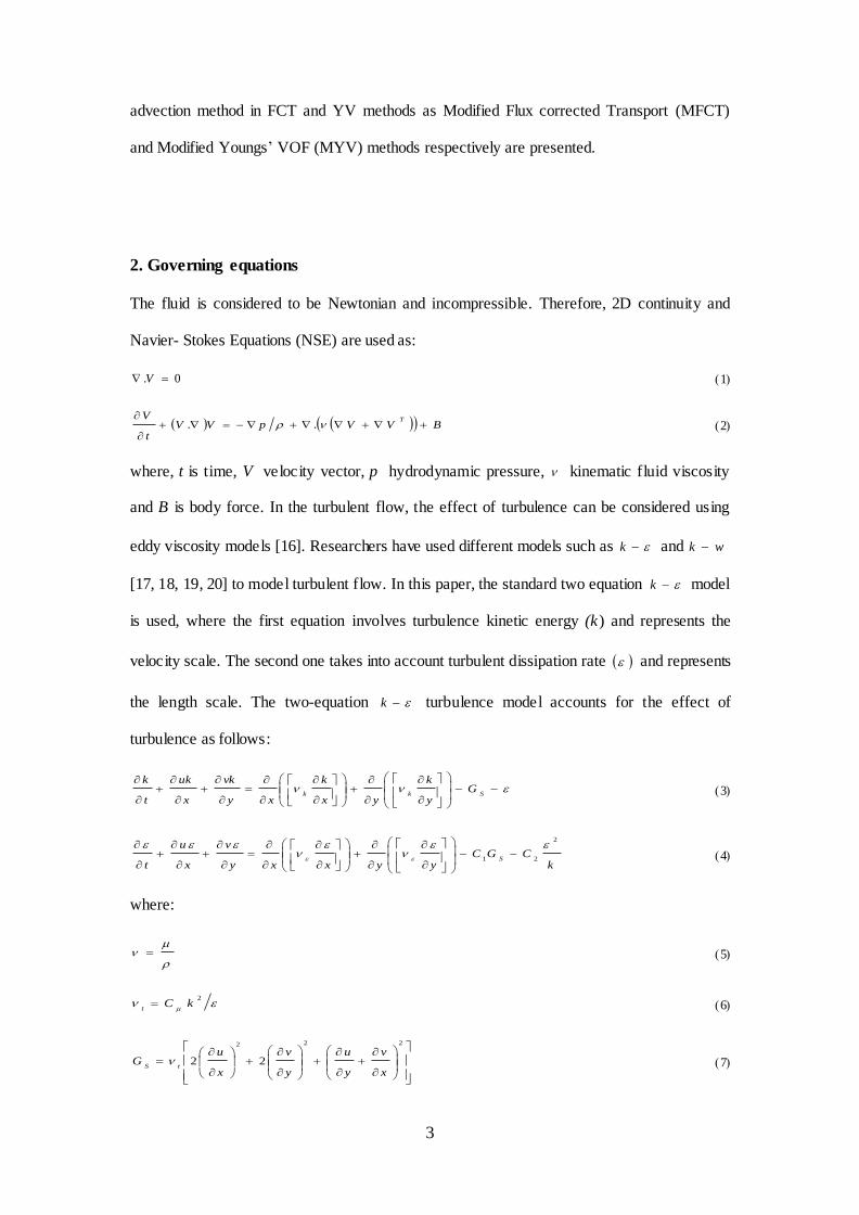
2. Governing equations

The fluid is considered to be Newtonian and incompressible. Therefore, 2D continuity and

Navier- Stokes Equations (NSE) are used as:

0. V (1 )

BVVpVVt

V T

.. (2)

where, t is time, V velocity vector, p hydrodynamic pressure, kinematic fluid viscosity

and B is body force. In the turbulent flow, the effect of turbulence can be considered using

eddy viscosity models [16]. Researchers have used different models such as k and wk

[17, 18, 19, 20] to model turbulent flow. In this paper, the standard two equation k model

is used, where the first equation involves turbulence kinetic energy (k) and represents the

velocity scale. The second one takes into account turbulent dissipation rate and represents

the length scale. The two-equation k turbulence model accounts for the effect of

turbulence as follows:

SkkG

y

k

yx

k

xy

vk

x

uk

t

k (3)

kCGC

yyxxy

v

x

u

tS

2

21

(4)

where:

(5)

2kC

t (6)

222

22x

v

y

u

y

v

x

uG

tS (7)

4

k

t

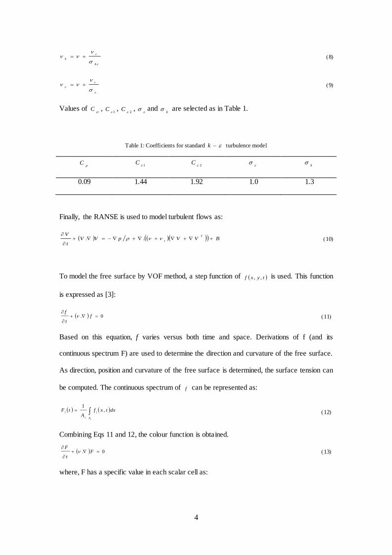
k (8)

t (9)

Values of

C , 1

C , 2

C ,

and k

are selected as in Table 1.

Table 1: Coefficients for standard k turbulence model

C

1C

2C

k

0.09 1.44 1.92 1.0 1.3

Finally, the RANSE is used to model turbulent flows as:

BVVpVVt

V T

t

.. (10)

To model the free surface by VOF method, a step function of tyxf ,, is used. This function

is expressed as [3]:

0.

f

t

f (11)

Based on this equation, f varies versus both time and space. Derivations of f (and its

continuous spectrum F) are used to determine the direction and curvature of the free surface.

As direction, position and curvature of the free surface is determined, the surface tension can

be computed. The continuous spectrum of f can be represented as:

iA

i

i

idxtxf

AtF ,

1 (12)

Combining Eqs 11 and 12, the colour function is obtained.

0.

F

t

F (13)

where, F has a specific value in each scalar cell as:

5

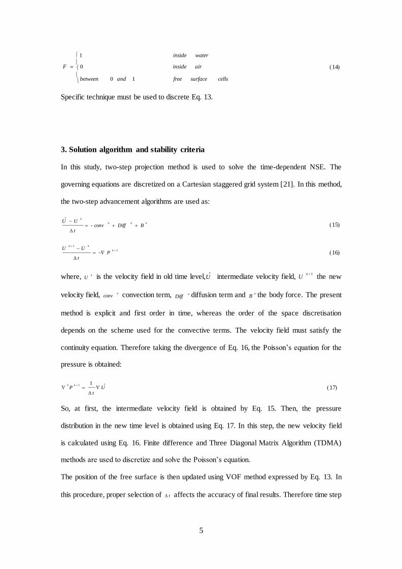
cellssurfacefreeandbetween

airinside

waterinside

F

10

0

1

(14)

Specific technique must be used to discrete Eq. 13.

3. Solution algorithm and stability criteria

In this study, two-step projection method is used to solve the time-dependent NSE. The

governing equations are discretized on a Cartesian staggered grid system [21]. In this method,

the two-step advancement algorithms are used as:

nnn

n

BDiffconvt

UU

ˆ (15)

1

1

n

nn

Pt

UU (16)

where, nU is the velocity field in old time level,U intermediate velocity field,

1nU the new

velocity field, nconv convection term, n

Diff diffusion term and nB the body force. The present

method is explicit and first order in time, whereas the order of the space discretisation

depends on the scheme used for the convective terms. The velocity field must satisfy the

continuity equation. Therefore taking the divergence of Eq. 16, the Poisson’s equation for the

pressure is obtained:

Ut

Pn ˆ

112

(17)

So, at first, the intermediate velocity field is obtained by Eq. 15. Then, the pressure

distribution in the new time level is obtained using Eq. 17. In this step, the new velocity field

is calculated using Eq. 16. Finite difference and Three Diagonal Matrix Algorithm (TDMA)

methods are used to discretize and solve the Poisson’s equation.

The position of the free surface is then updated using VOF method expressed by Eq. 13. In

this procedure, proper selection of t affects the accuracy of final results. Therefore time step

6

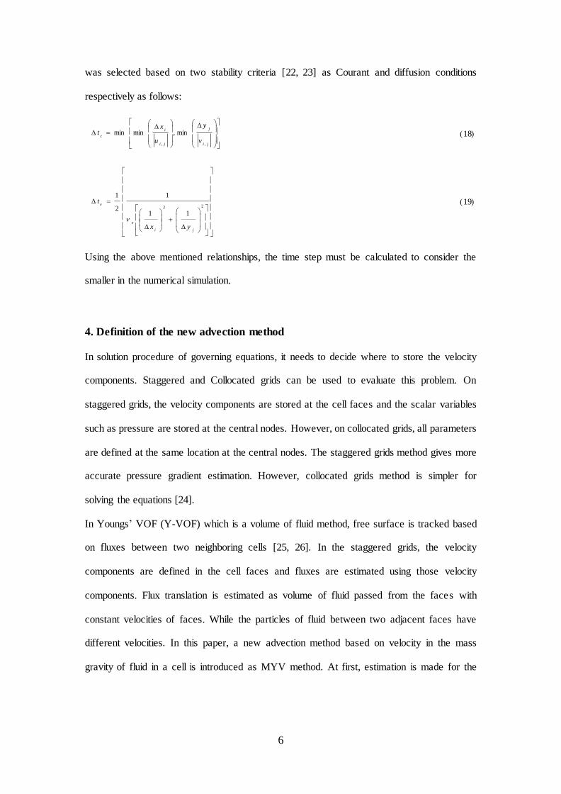
was selected based on two stability criteria [22, 23] as Courant and diffusion conditions

respectively as follows:

ji

j

ji

i

c

v

y

u

xt

,,

min,minmin

(18)

22

11

1

2

1

ji

e

yx

t

(19)

Using the above mentioned relationships, the time step must be calculated to consider the

smaller in the numerical simulation.

4. Definition of the new advection method

In solution procedure of governing equations, it needs to decide where to store the velocity

components. Staggered and Collocated grids can be used to evaluate this problem. On

staggered grids, the velocity components are stored at the cell faces and the scalar variables

such as pressure are stored at the central nodes. However, on collocated grids, all parameters

are defined at the same location at the central nodes. The staggered grids method gives more

accurate pressure gradient estimation. However, collocated grids method is simpler for

solving the equations [24].

In Youngs’ VOF (Y-VOF) which is a volume of fluid method, free surface is tracked based

on fluxes between two neighboring cells [25, 26]. In the staggered grids, the velocity

components are defined in the cell faces and fluxes are estimated using those velocity

components. Flux translation is estimated as volume of fluid passed from the faces with

constant velocities of faces. While the particles of fluid between two adjacent faces have

different velocities. In this paper, a new advection method based on velocity in the mass

gravity of fluid in a cell is introduced as MYV method. At first, estimation is made for the

7

interface orientation . The interface within a cell is then approximated by a straight line

segment with orientation as shown in Fig. 1.

Fig. 1: Interface orientation in a free surface (i,j ) cell

Free surface cuts the cell in such a way that the fractional fluid volume is given by F(i,j). The

geometry of the fluid resulting from this reconstruction is then used to determine the fluxes

through any side on which the velocity is directed out of the cell. For example, flux from right

cell face (r

F ) for cell shown in Fig. 2-a can be estimated as:

dxSdtjiUifdydxjiF

dxSdtjiUifdySdxS

dtjiUdtjiU

F

b

br

b

r

),(**),(

),(*),(

2),(2

1

(20)

Similarly, it is assumed that fluid is passed from cell face with constant velocity equal to cell

face velocity. So, in the developed model, fluxes are calculated based on horizontal and

vertical velocity of mass center of fluid cells. Fig. 2 shows new arrangement of velocity in

MYV method.

8

(a) (b)

(c) (d)

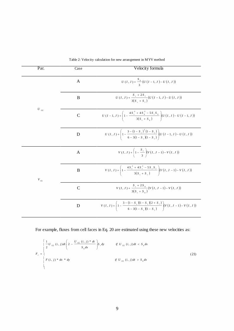
Fig. 2: Definition of velocity arrangement in new advection algor ithm in MYV method

The new equations of horizontal and vertical velocity CGCG

VandU in the mass center are

estimated using equations summarized in Table 2.

9

Table 2: Velocity calculation for new arrangement in MYV method

Par. Case Velocity formula

CGU

A JIUJIUS

JIUb

,,13

),(

B

JIUJIUSS

SSJIU

lr

lr,,1

3

2),(

C

JIUJIUSS

SSSSJIU

bt

btbt,1,

3

5441),1(

22

D

JIUJIU

SS

SSJIU

lt

lt,,1

1136

1131),(

2

CGV

A JIVJIVS

JIVl

,1,3

1),(

B

JIVJIVSS

SSSSJIV

rl

lrrl,1,

3

5441),(

22

C

JIVJIVSS

SSJIV

bt

bt,1,

3

2),(

D

JIVJIV

SS

SSSJIV

lt

llt,1,

1136

21131),(

For example, fluxes from cell faces in Eq. 20 are estimated using these new velocities as:

dxSdtjiUifdydxjiF

dxSdtjiUifdySdxS

dtjiUdtjiU

F

bCG

bCGr

b

CG

CG

r

),(**),(

),(*),(

2),(2

1

(21)

10

5. Model validation

To validate the modified model, a series of standard tests such as lid-driven cavity, sloshing

problem, constant unidirectional velocity field, shear test and dam break over a dry bed was

carried out.

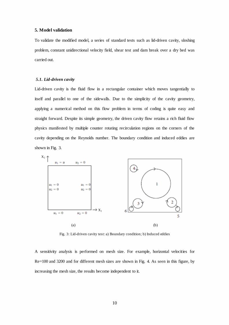
5.1. Lid-driven cavity

Lid-driven cavity is the fluid flow in a rectangular container which moves tangentially to

itself and parallel to one of the sidewalls. Due to the simplicity of the cavity geometry,

applying a numerical method on this flow problem in terms of coding is quite easy and

straight forward. Despite its simple geometry, the driven cavity flow retains a rich fluid flow

physics manifested by multiple counter rotating recirculation regions on the corners of the

cavity depending on the Reynolds number. The boundary condition and induced eddies are

shown in Fig. 3.

(a) (b)

Fig. 3: Lid-driven cavity test: a) Boundary condition; b) Induced eddies

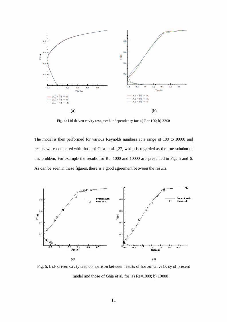
A sensitivity analysis is performed on mesh size. For example, horizontal velocities for

Re=100 and 3200 and for different mesh sizes are shown in Fig. 4. As seen in this figure, by

increasing the mesh size, the results become independent to it.

X1

X2

11

(a) (b)

Fig. 4: Lid-driven cavity test, mesh independency for: a) Re=100; b) 3200

The model is then performed for various Reynolds numbers at a range of 100 to 10000 and

results were compared with those of Ghia et al. [27] which is regarded as the true solution of

this problem. For example the results for Re=1000 and 10000 are presented in Figs 5 and 6.

As can be seen in these figures, there is a good agreement between the results.

(a) (b)

Fig. 5: Lid- driven cavity test, comparison between results of horizontal velocity of present

model and those of Ghia et al. for: a) Re=1000; b) 10000

12

(a) (b)

Fig. 6: Lid- driven cavity test, comparison between results of vertical velocity of present

model and those of Ghia et al. for: a) Re=1000; b) 10000

5.2. Sloshing problem

Sloshing of a liquid low amplitude wave under forced movement is another problem to test

the interfacial flow solver. In this test a rectangular tank with a width of 0.9 m and a water

depth of 0.6 m was exposed to a horizontal periodic sway motion as tX 5.5sin002.0 .

Therefore tax

5.5sin0605.0 was considered as exciting acceleration. The displacement

of a node on the free surface in contact with right hand sidewall was calculated by the

model and compared with those of Nakayama and Washizu [28] in Fig. 7. The existence of a

good agreement between results can be seen in this figure.

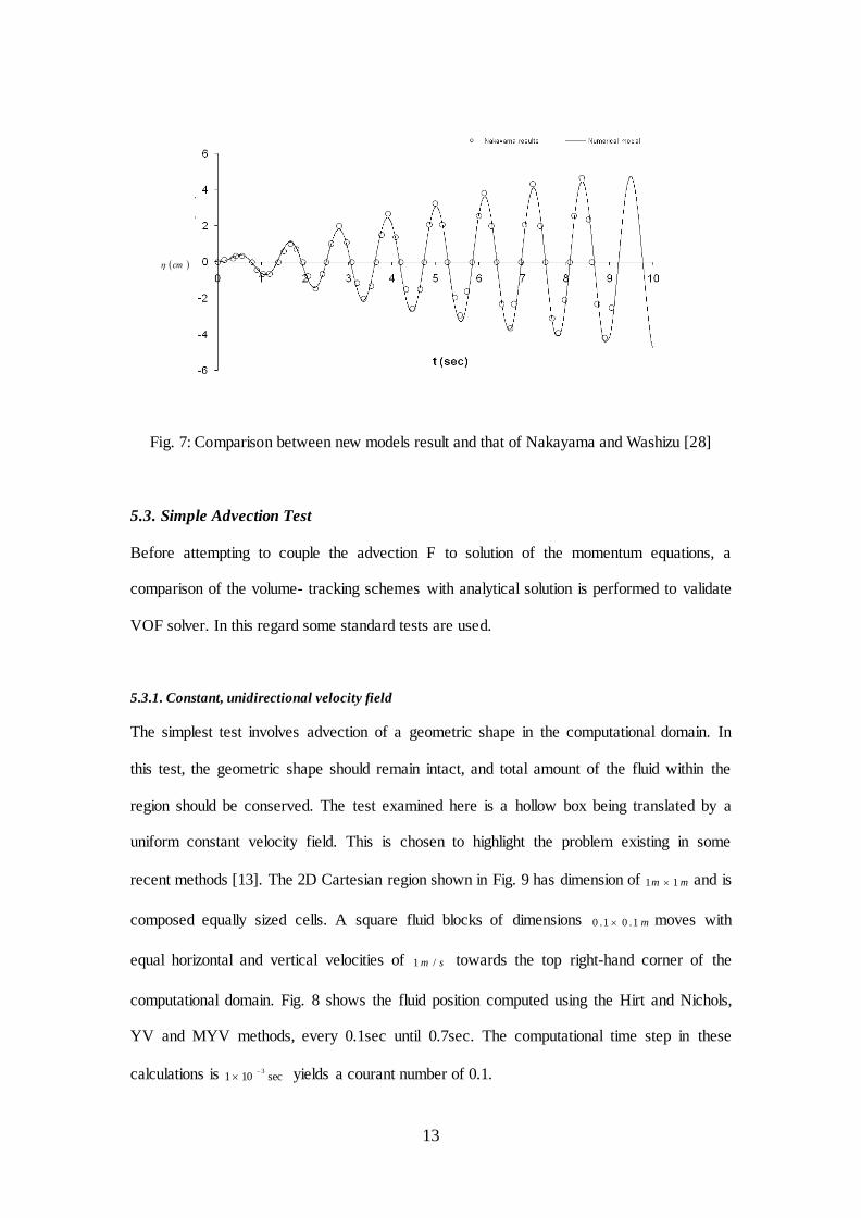
13

Fig. 7: Comparison between new models result and that of Nakayama and Washizu [28]

5.3. Simple Advection Test

Before attempting to couple the advection F to solution of the momentum equations, a

comparison of the volume- tracking schemes with analytical solution is performed to validate

VOF solver. In this regard some standard tests are used.

5.3.1. Constant, unidirectional velocity field

The simplest test involves advection of a geometric shape in the computational domain. In

this test, the geometric shape should remain intact, and total amount of the fluid within the

region should be conserved. The test examined here is a hollow box being translated by a

uniform constant velocity field. This is chosen to highlight the problem existing in some

recent methods [13]. The 2D Cartesian region shown in Fig. 9 has dimension of mm 11 and is

composed equally sized cells. A square fluid blocks of dimensions m1.01.0 moves with

equal horizontal and vertical velocities of sm /1 towards the top right-hand corner of the

computational domain. Fig. 8 shows the fluid position computed using the Hirt and Nichols,

YV and MYV methods, every 0.1sec until 0.7sec. The computational time step in these

calculations is sec1013

yields a courant number of 0.1.

cm

14

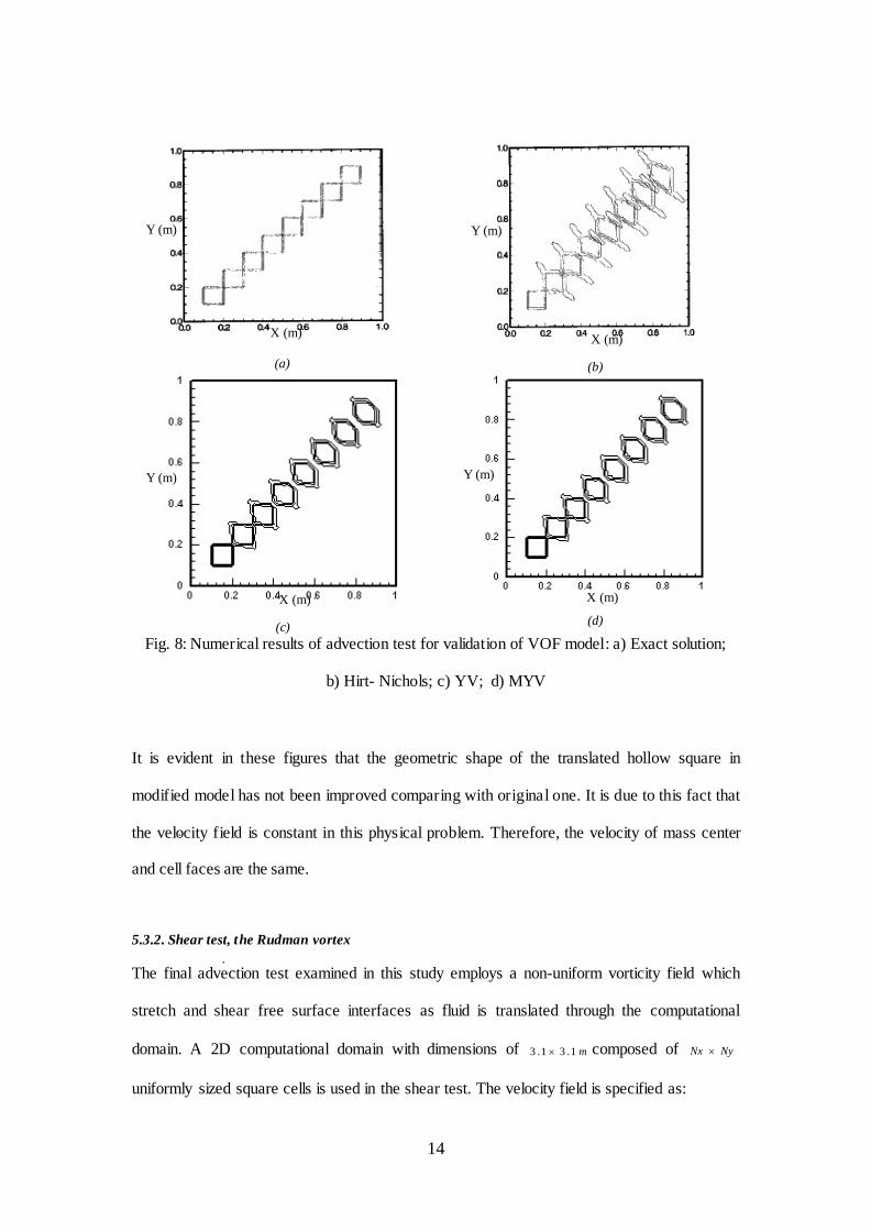
(b)

(a)

(d)

(c) Fig. 8: Numerical results of advection test for validation of VOF model: a) Exact solution;

b) Hirt- Nichols; c) YV; d) MYV

It is evident in these figures that the geometric shape of the translated hollow square in

modified model has not been improved comparing with original one. It is due to this fact that

the velocity field is constant in this physical problem. Therefore, the velocity of mass center

and cell faces are the same.

5.3.2. Shear test, the Rudman vortex

The final advection test examined in this study employs a non-uniform vorticity field which

stretch and shear free surface interfaces as fluid is translated through the computational

domain. A 2D computational domain with dimensions of m1.31.3 composed of NyNx

uniformly sized square cells is used in the shear test. The velocity field is specified as:

X (m) X (m)

X (m)

X (m) X (m)

Y (m) Y (m)

Y (m) Y (m)

.

.

15

yxAyxU cossin, (22)

yxAyxV sincos, (23)

Which A equals 1 for first N computational time step, and -1 for the second N time steps. The

initial fluid geometry is a circle of radius m2.0 . Time step is selected by courant number of

0.25 based on the maximum velocity within the computational domain. A sensitivity analysis

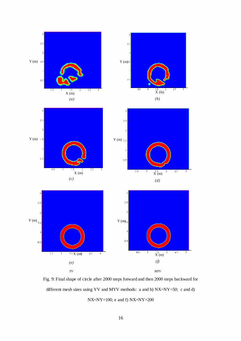
is performed on mesh sizes. The final shape of circle after 2000 steps forward and then 2000

steps backward for different mesh numbers are estimated using different VOF methods. The

results are presented in Fig 9.

16

(a)

(b)

(c)

(d)

(e)

(f)

YV MYV

Fig. 9: Final shape of circle after 2000 steps forward and then 2000 steps backward for

different mesh sizes using YV and MYV methods: a and b) NX=NY=50; c and d)

NX=NY=100; e and f) NX=NY=200

X (m)

X (m) X (m)

Y (m)

Y (m) Y (m)

Y (m)

X (m)

X (m)

Y (m)

X (m)

Y (m)

17

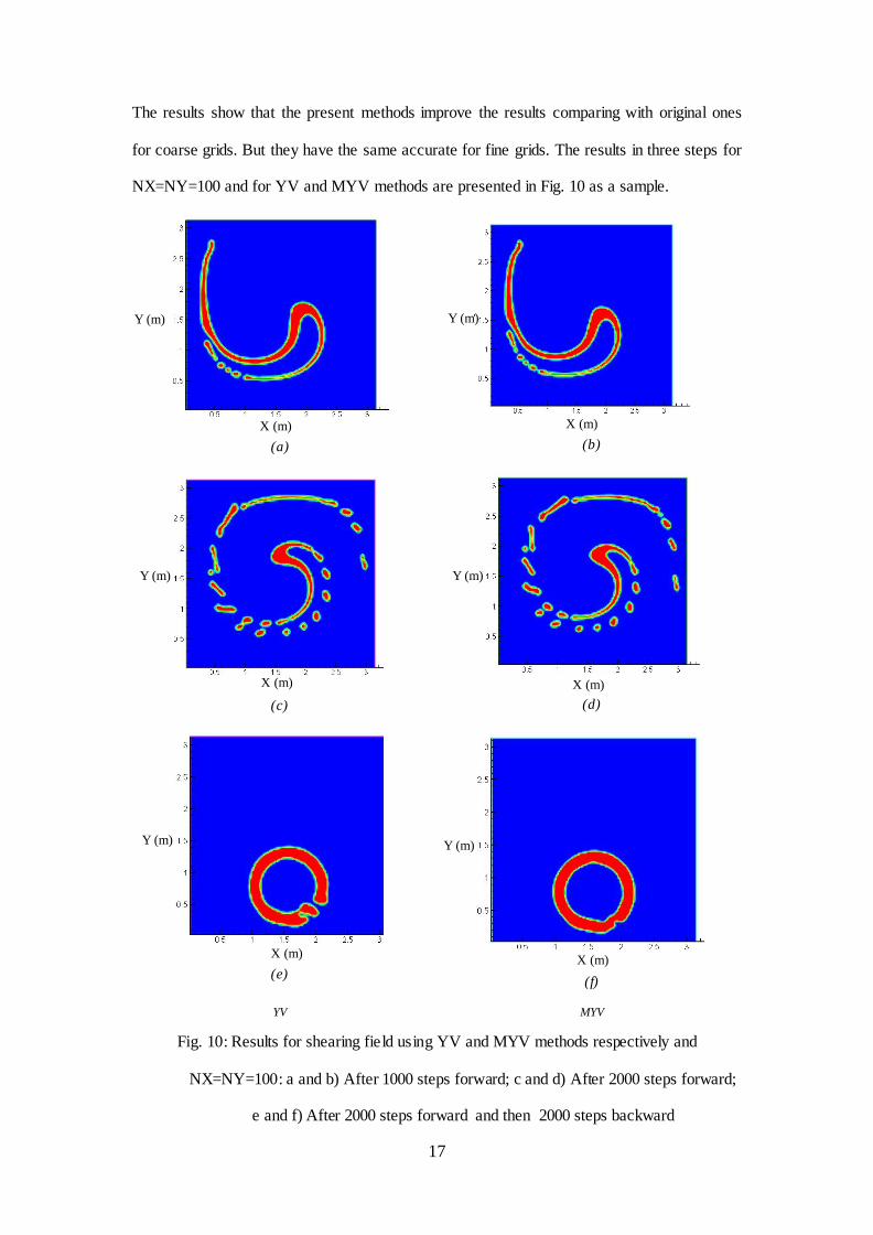
The results show that the present methods improve the results comparing with original ones

for coarse grids. But they have the same accurate for fine grids. The results in three steps for

NX=NY=100 and for YV and MYV methods are presented in Fig. 10 as a sample.

(a)

(b)

(c)

(d)

(e)

(f)

YV MYV

Fig. 10: Results for shearing field using YV and MYV methods respectively and

NX=NY=100: a and b) After 1000 steps forward; c and d) After 2000 steps forward;

e and f) After 2000 steps forward and then 2000 steps backward

X (m)

X (m) X (m)

Y (m)

Y (m) Y (m)

Y (m)

X (m)

X (m)

Y (m)

X (m)

Y (m)

18

5.4. Dam break over a dry bed

Another test problem used for free surface case is the collapse of water column over a dry

bed. This problem was first studied and used as benchmark by the developers of SOLA-VOF

(Nichols et al. [4]). It is a very useful benchmark providing extreme conditions to assess the

numerical stability as well as the capability of the model to treat the free surface problem. In

this test, a square computational domain with a length and height of 22.8 cm is set. A water

column with the width of L=5.7 cm and height of 2L is assumed at the left of the

computational domain surrounded by walls with no-slip boundary condition. The spatial step

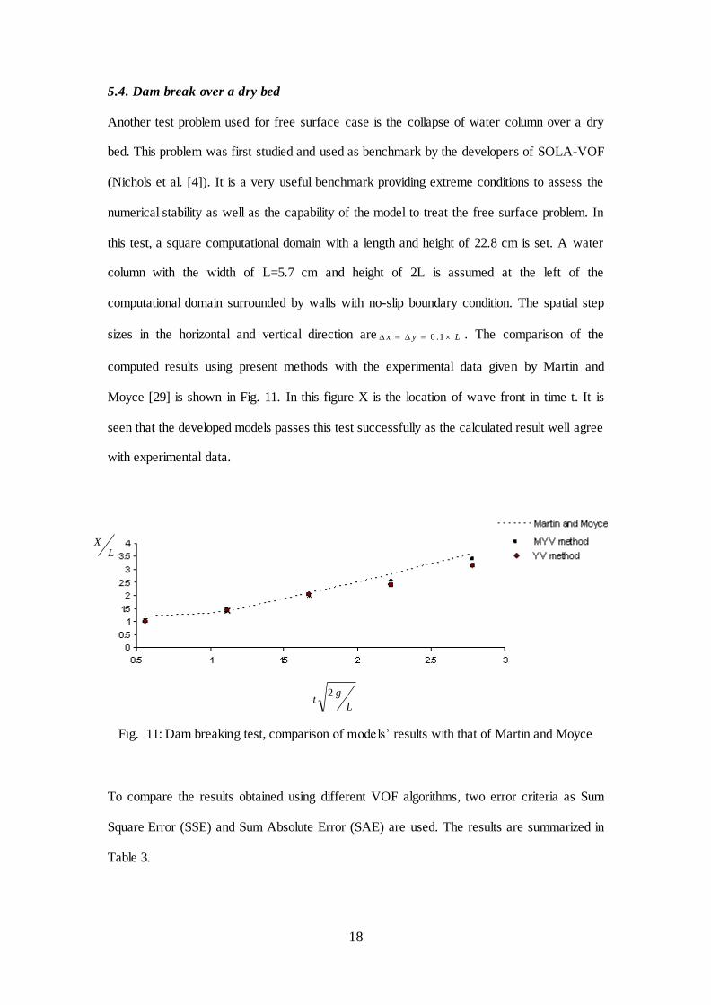
sizes in the horizontal and vertical direction are Lyx 1.0 . The comparison of the

computed results using present methods with the experimental data given by Martin and

Moyce [29] is shown in Fig. 11. In this figure X is the location of wave front in time t. It is

seen that the developed models passes this test successfully as the calculated result well agree

with experimental data.

Fig. 11: Dam breaking test, comparison of models’ results with that of Martin and Moyce

To compare the results obtained using different VOF algorithms, two error criteria as Sum

Square Error (SSE) and Sum Absolute Error (SAE) are used. The results are summarized in

Table 3.

L

gt

2

LX

19

Table 3: Comparison of SSE and SAE errors of different VOF algorithms in Dam break test

MYV YV Error

0.15 0.25 SSE

0.81 0.97 SAE

6. Discussion and conclusion

In this research, modified Volume of Fluid method based on Youngs’ VOF algorithm denoted

by Modified Youngs’ VOF (MYV) method is presented. In this method, for staggered grids

fluxes to neighboring cells are estimated based on cell face velocities. However in practice

these particles have a variable velocity between velocities of two adjacent cell faces. In the

developed model, the velocity in mass center of fluid cell, is estimated and used to calculate

fluxes from cell faces. To validate the modified model, a serious of standard tests such as Lid-

driven cavity, Sloshing problem, Constant unidirectional velocity field, Shear test and Dam

break over a dry bed was carried out. The results showed that in some cases such as Constant,

unidirectional velocity field, geometric shape of the translated hollow square in modified

model has not been improved comparing with original one. It is due to this fact that the

velocity field is constant in this physical problem. Therefore velocities of mass center and cell

faces are the same. In some other cases such as Shear test, modified model improves the

results. However, they have the same accuracy in fine grids. In Dam break test, present

method improves the results. Therefore, the MYV method is suggested as a new VOF

algorithm which models the free surface problems more accurately.

20

7. References

[1] Burnner, B. and Tryggavson, G.: Direct Numerical Simulation of three- dimensional

bubbly flow. Physics of Fluids (Letter) 111, 1967-1969 (1999).

[2] Lafaurie, B. Nardone, C. Scardovelli, R. Zaleski S. and Zanetti, G.: Modeling merging and

fragmentation in multiphase flows with SURFER. Journal of Computational physics.

113, 134-147 (1994).

[3] Noh, W.F. and Woodward, P.: SLIC (Simple line Interface Calculation). in A. I. van

Dooren and M.J. Baines (eds), Lecture notes in physics, Springer, New York. 59,

273-285 (1982).

[4] Nichols, B.D. Hirt, C.W. and Hotchkiss, R.S.: SOLA- VOF: a solution algorithm for

transient fluid flow with multiple free boundaries. Technical Report LA-8355, Los

Alamos Scientific Laboratory. (1980).

[5] Torrey, M.D. Cloutman, L.D. and Hirt, C.W.: NASA-VOF2D: a computer program for

incompressible flows with free surface. Technical report LA-10462-MS, Los Alamos

Scientific Laboratory. (1985).

[6] Hirt, C.V. and Nichols, B.D.: Volume of Fluid (VOF) method for the dynamics of free

boundaries. Journal of computational physics. 39, 201-225 (1981).

[7] Youngs, D.L.: Time-depend multi- material flow with large fluid distortion. In K. W.

Morton and M. J. Baines (eds), Numerical Methods for Fluid dynamics, Academic,

New York. 273-285 (1985).

[8] Rudman, M.: Volume-tracking methods for interfacial flow calculations. International

Journal for Numerical Methods in Fluids. 24, 671-691 (1997).

[9] Duff, E.S.: Fluid flows aspects of solidification modeling: simulation of low pressure Die

casting. PhD Thesis, University of Queensland, Brisbane. (1999).

[10] Rider, W.J. and Kothe, B.D.: Reconstructing volume tracking, Journal of Computational

physics. 141, 112-152 (1998).

21

[11] Harvie, D.J.E. and Fletcher, D.F.: A new volume of fluid advection algorithm: the

defined donating region scheme. International Journal of Numerical Methods in

Fluid. 35, 151-172 (2001).

[12] Harvie, D.J.E. and Fletcher, D.F.: A new volume of fluid advection algorithm: the stream

scheme. Journal of computational physics. 162, 1-32 (2000).

[13] Geuyffier, D. Li, J. Nadim, A. Scardovelli, R. and Zaleski, S.: Volume- of-fluid interface

tracking with smoothed surface stress methods for three- dimensional flows. Journal

of computational physics. 152, 423-456 (1999).

[14] Scardovelli, R. and Zaleski, S.: NOTE: analytical relations connecting linear interfaces

and volume fractions in rectangular grid. Journal of Computational physics. 164, 228-

237 (2000).

[15] Scardovelli, R. and Zaleski, S.: Interface reconstruction with least-square fit and split

Eulerian- Lagrangian advection. Internatioanl Journal of Numerical Methods in

Fluids. 41, 251-274 (2003).

[16] Rafei, R. : Numerical solution of incompressible 3D turbulent flow in a spiral channel.

M.Sc. thesis, Amirkabir University of Technology, Iran, Tehran. (2004).

[17] Li, C.W. and Zang, Y.F.: Simulation of free surface recirculating flows in semi-enclosed

water bodies by a wk model. Applied Mathematical modeling. 22, 153-164

(1998).

[18] Gao, H. Gu, H.Y. and Guo, L.J.: Numerical study of stratified oil-water two-phase

turbulent flow in a horizontal tube. Int J Heat Mass Transfer. 46, 749-754 (2003).

[19] Ren, B. and Wang, Y.: Numerical simulation of random wave slamming on structures in

the splash zone. Ocean Engineering. 31, 547-560 (2004).

[20] Shen, Y.M. Ng, C.O. and Zheng, Y.H.: Simulation of wave propagation over a

submerged bar using the VOF method with a two-equation k turbulence

modeling. Ocean Engineering. 31, 87-95 (2004).

22

[21] Guizien, K. and Barthélemy, E.: Short waves modulations by large free surface solitary

waves: Experiments and models. Phys. Fluids. 13, 3624-3635 (2000).

[22] Renouard, D.P. Seabra-Santos, F.J. and Temperville, A.M.: Experimental study of the

generation, damping and reflection of a solitary wave. Dynamics of Atm. and Oceans.

9, 341-358 (1985).

[23] Boussinesq, M.J.: Théorie de l’intumescence liquide, appelée onde solitaire ou de

translation. se propageant dans un canal rectangulaire. C.-R. Acad. Sci. Paris, 755-

759 (1871).

[24] Ketabdari, M.J. and Saghi, H.: Large Eddy Simulation of Laminar and Turbulent Flow

on Collocated and Staggered Grids, ISRN Mechanical Engineering, vol. 2011, Article

ID 809498, 13 pages, (2011). doi:10.5402/2011/809498.

[25] Ketabdari, M.J. Nobari, M.R.H. and Moradi Larmaei, M.: Simulation of waves group

propogation and breaking in coastal zone using a Navier- Stokes solver with an

improved VOF free surface treatment. Applied Ocean Research. 30, 130-143 (2008).

[26] Nobari, M.R.H. Ketabdari, M.J. and Moradi Larmaei, M.: A modified Volume of Fluid

advection method for uniform Cartesian grids. Applied Mathematical Modeling. 33,

2298–2310 (2009).

[27] Ghia, U. Ghia, K.N. and Shin, C.T.: High-Re Solutions for Incompressible Flow Using

the Navier-Stokes Equations and a Multigrid Method. Journal of Computational

Physics. 48, 387-411 (1982).

[28] Nakayama, T. and Washizu, K.: Boundary Element Analysis of Nonlinear Sloshing

Problems. Published in Developments in Boundary Element Method-3, Bauerjee P.

K, Mukherjee S., and Elsevier Applied Science Publishers, Newyork, (1984).

[29] Martin, J.C. and Moyce, W.J.: An experimental study of the collapse of liquid columns

on a rigid horizontal plane. Philosophical Transaction of the Royal Society of

London. 244, 312-324 (1952).