AIR TOXIC EMISSIONS FROM MOBILE SOURCES IN WINTER

By

FARAH N. ABEDIN

A thesis submitted in partial fulfillment of the requirements for the degree of

MASTER OF SCIENCE IN ENVIRONMENTAL ENGINEERING

WASHINGTON STATE UNIVERSITY Department of Civil and Environmental Engineering

DECEMBER 2011

ii

To the Faculty of Washington State University:

The members of the Committee appointed to examine the thesis of

FARAH N. ABEDIN find it satisfactory and recommend that it be

accepted.

Bertram T. Jobson, Ph.D., Chair

Brian K. Lamb, Ph. D.

Joseph K. Vaughan, Ph.D.

iii

ACKNOWLEDGEMENT

Many people have helped me in the process of writing this thesis. I would like to take this

opportunity to thank some of the individuals.

First and foremost, I would like to thank my academic advisor, Dr. Tom Jobson. He has

been an amazing guide and an excellent teacher throughout this whole process. He never

shied away from my numerous silly questions and showed extraordinary patience while

explaining things to me. He always encouraged me to look at the big picture, beyond all

the numbers and equations. I have learned a lot from him about chemistry, logic and

life’s intricate philosophy. I feel very lucky that I got to work with him for the past two

years.

I would also like to thank my thesis committee members, Drs. Brian Lamb and Joseph

Vaughan. They have helped me, along with my advisor, to achieve my goals in my

research and guided me through some rocky territories. I thank Dr. Brian Lamb for taking

an interest in my research and for encouraging me to explore the possibilities beyond this

thesis. I cannot thank Dr. Vaughan enough for helping me understand some of the key

aspects of AIRPACT. He patiently guided me through the process of extracting the

modeled data. I am deeply grateful for his insights and suggestions on writing this

manuscript.

Many thanks go to past and present graduate students of LAR. I am very grateful to my

fellow graduate students and office mates, Will Wallace and Matt Erickson for helping

iv

me with Igor codes to manipulate my data. Had they not, I would be still crunching

numbers the old way and develop a permanent carpal tunnel syndrome.

I would specially like to thank Rasa Grivicke, Kara Yedinak and Celia Faiola for all the

conversations we had over the years about school and beyond. I would also like to show

appreciation to my fabulous office mates: Andrew Rengel, Vincent Fricaud, Sarah

Waldo, Rodrigo Gonzalez-Abraham, George Mwaniki and Farren Herron-Thorpe. Thank

you all for your friendship and support.

Lastly, I would like to thank my family and friends, around the globe, for their endless

love, support and patience.

v

AIR TOXIC EMISSIONS FROM MOBILE SOURCES IN WINTER

Abstract

by Farah N. Abedin, M.S. Washington State University

December 2011

Chair: Bertram T. Jobson

The US Environmental Protection Agency has labeled six air toxics to be the most

hazardous to human health, including formaldehyde, acetaldehyde and benzene. In urban

areas, these are mainly emitted by vehicles when lower temperature inhibits biogenic

emissions. Among these toxics benzene is a well known carcinogen and the aldehydes

(formaldehyde and acetaldehyde) can also contribute to ground level ozone formation

besides affecting human health. To estimate toxic emissions from mobile sources, toxic

assessment programs can use emission ratios along with ambient monitoring data. In this

study, emission ratios relative to vehicle exhaust tracers (CO and NOX) were calculated

by using parameters from regression analysis.

Formaldehyde, acetaldehyde and benzene along with other volatile organic compounds

(VOCs) and trace gases (CO, NOX) were measured in winter from December 2008 to

January 2009 as a part of the Treasure Valley PM2.5 campaign in Meridian, Idaho. By

analyzing the morning rush hour period, we found that the emissions ratios with respect

to CO were 3.30 ± 0.29 pptv/ppbv, 2.11 ± 0.20 pptv/ppbv and 1.30 ± 0.07 pptv/ppbv for

formaldehyde, acetaldehyde and benzene respectively. The emission ratios with respect

vi

to NOX were 11.9 ± 1.2 pptv/ppbv, 7.99 ± 1.03 pptv/ppbv and 5.06 ± 0.47 pptv/ppbv for

formaldehyde, acetaldehyde and benzene respectively. These emission ratios with CO

were found to be in reasonable agreement with previous studies done in various cities.

The measured emission ratios were also compared with calculated ones from modeled

data generated by AIRPACT-3. The measured emission ratios, for aldehydes with respect

to NOX and for benzene with respect to CO, were comparable to the modeled ones. The

good agreement for AIRPACT versus observations, for NOX correlations compared to

those with CO, suggests that the CO emission from the model is over predicted by a

factor of 5.2.

vii

TABLE OF CONTENTS

ACKNOWLEDGEMENT ................................................................................................ iii

ABSTRACT .................................................................................................................... v-vi

LIST OF TABLES ........................................................................................................... viii

LIST OF FIGURES .............................................................................................................x

CHAPTER 1: INTRODUCTION ........................................................................................1

1.1. Air toxics ..............................................................................................................1

1.2.Sources of air toxics ...............................................................................................3

1.2.1. Acetaldehyde..................................................................................................5

1.2.2. Benzene ..........................................................................................................6

1.2.3. Formaldehyde ................................................................................................7

1.3. Air toxics in urban areas ......................................................................................10

1.4. Modeling air toxics ..............................................................................................14

1.5. Objective..............................................................................................................16

CHAPTER 2: EXPERIMENTAL......................................................................................17

2.1. Site description ....................................................................................................17

2.2. Measurements ......................................................................................................19

CHAPTER 3: RESULTS AND DISCUSSION .................................................................23

3.1. Data description ...................................................................................................23

3.2. Morning rush hour Analysis ................................................................................34

3.3. Selection criteria for morning rush hour periods .................................................37

3.4. Air toxics correlation analysis for rush hour periods ..........................................39

3.4.1. Correlation with CO .....................................................................................39

viii

3.4.1.1. Formaldehyde ....................................................................................39

3.4.1.2. Acetaldehyde .....................................................................................44

3.4.1.3. Benzene .............................................................................................47

3.4.1.4. Other species......................................................................................50

3.4.1.4.1. m/z = 69 .....................................................................................50

3.4.1.4.2. m/z = 137 ...................................................................................51

3.4.1.4.3. Aromatics ...................................................................................52

3.4.2. Correlation with NOX...................................................................................55

3.4.2.1. Formaldehyde ....................................................................................55

3.4.2.2. Acetaldehyde .....................................................................................58

3.4.2.3. Benzene .............................................................................................62

3.4.2.4. Other species......................................................................................65

3.4.2.4.1. m/z = 69 .....................................................................................66

3.4.2.4.2. m/z = 137 ...................................................................................67

3.4.2.4.3. Aromatics ...................................................................................68

3.5. Comparison to AIRPACT-3 ................................................................................70

3.5.1. Formaldehyde ..............................................................................................71

3.5.2. Acetaldehyde................................................................................................73

3.5.3. Benzene ........................................................................................................76

3.5.4. Aromatics .....................................................................................................77

3.6. Summary and discussion .....................................................................................80

CHAPTER 4: CONCLUSION ..........................................................................................85

BIBLIOGRAPHY ..............................................................................................................89

ix

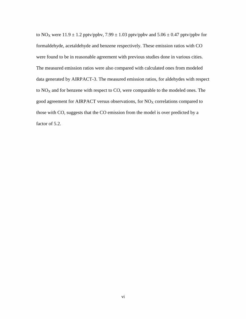
LIST OF TABLES

Table 1.1. List of EPA Mobile Source Air Toxics .............................................................2

Table 3.1. Summary of statistics of measured volatile organic compounds (VOCs) and

carbon monoxide and nitrogen oxides (5 - minute averages) ...........................................23

Table 3.2. Parameters for linear regressions of HCHO vs. CO for the selected morning

rush hour periods. The average temperature and relative humidity are included .............40

Table 3.3. Parameters for linear regressions of HCHO vs. CH3CHO for the selected

morning rush hour periods .................................................................................................43

Table 3.4. Parameters for linear regressions of CH3CHO vs. CO for the selected morning

rush hour periods................................................................................................................46

Table 3.5. Parameters for linear regressions of benzene vs. CO for the selected morning

rush hour periods................................................................................................................48

Table 3.6. Parameters for linear regressions of aromatics vs. CO for the selected morning

rush hour periods................................................................................................................54

Table 3.7. Parameters for linear regressions of HCHO vs. NOx for the selected morning

rush hour periods. The average temperature and relative humidity are included .............56

Table 3.8. Parameters for linear regressions of CH3CHO vs. NOx for the selected

morning rush hour periods .................................................................................................60

x

Table 3.9. Parameters for linear regressions of benzene vs. NOX for the selected morning

rush hour periods................................................................................................................63

Table 3.10. Parameters for linear regressions of unknown #2 (m/z =137) vs. NOX for the

selected morning rush hour periods ...................................................................................67

Table 3.11. Parameters for linear regressions of aromatics vs. NOX for the selected

morning rush hour periods .................................................................................................69

Table 3.12. Emission ratios of VOCs from Meridian, Idaho and modeled data from

AIRPACT-3 ......................................................................................................................82

Table 3.13. Emission ratios of air toxics with respect to CO from Meridian, Idaho and

other cities. Units are in pptv/ppbv CO .............................................................................84

xi

LIST OF FIGURES

Figure 1.1. Sources of urban air toxics ................................................................................4

Figure 1.2. Block diagram of O3 production driven by HCHO, HOX and NOX chemistry.

............................................................................................................................................13

Figure 2.1 Map of the study site in Meridian, Idaho. .......................................................18

Figure 2.2. Close-up of the measurement trailer equipped with the instruments ..............20

Figure 3.1.1. Plots of 5 - minute averaged data of temperature, relative humidity,

formaldehyde (HCHO), nitrogen oxides (NOX) and carbon monoxide (CO) mixing ratios

in Meridian, Idaho, from 1 December, 2008 to 31 January, 2009. ...................................25

Figure 3.1.2. Plots of 5 - minute averaged data of acetaldehyde, acetone, acetonitrile and

benzene mixing ratios in Meridian, Idaho, from 1 December, 2008 to 31 January, 2009.

............................................................................................................................................26

Figure 3.1.3. Plots of 5 - minute averaged data of C2-benzene, C3-benzene, C3-benzene

and methanol mixing ratios in Meridian, Idaho, from 1 December, 2008 to 31 January,

2009. ..................................................................................................................................27

Figure 3.1.4. Plots of 5 - minute averaged data of naphthalene, pentenes, phenol and

toluene mixing ratios in Meridian, Idaho, from 1 December, 2008 to 31 January, 2009. 28

Figure 3.1.5. Plots of 5 - minute averaged data of unknown #1 (m69) and unknown #2

(m137) mixing ratios in Meridian, Idaho, from 1 December, 2008 to 31 January, 2009. 29

Figure 3.2. Diel profiles of formaldehyde, acetaldehyde, benzene and CO mixing ratio as

half hour averages ..............................................................................................................30

Figure 3.3. Wind rose plots showing wind speed and fractional occurrence of wind flow

direction in 30° increment bins for day and night during the entire campaign and the

stagnation period ...............................................................................................................31

xii

Figure 3.4.1. Plots of 5 - minute averaged mixing ratios of CO and formaldehyde as a

function of wind direction in 30° increment bins. ............................................................32

Figure 3.4.2. Plots of 5 - minute averaged mixing ratios of Acetaldehyde and Benzene as

a function of wind direction in 30° increment bins............................................................33

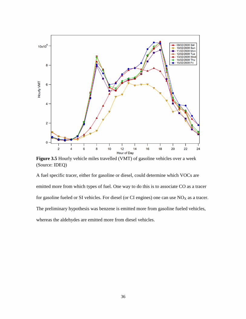
Figure 3.5. Hourly vehicle miles travelled (VMT) of gasoline vehicles over a week ......36

Figure 3.6. Hourly vehicle miles travelled (VMT) of diesel vehicles over a week ..........37

Figure 3.7. Relationships between HCHO and CO mixing ratios in Meridian, Idaho. ...39

Figure 3.8. Measured and calculated (using HCHO/CO ratio) HCHO mixing ratios ......41

Figure 3.9. Histogram plots of the ratio of observed and predicted (using HCHO/CO

ratio) formaldehyde mixing ratios ....................................................................................42

Figure 3.10. Relationships between formaldehyde and acetaldehyde mixing ratios .........43

Figure 3.11. Relationships between acetaldehyde and carbon monoxide mixing ratios in

Meridian, Idaho. ................................................................................................................44

Figure 3.12 Measured and calculated (using CH3CHO/CO ratio) CH3CHO mixing ratios.

............................................................................................................................................45

Figure 3.13. Histogram plots of the ratio of observed and predicted (using CH3CHO/CO

ratio) of acetaldehyde mixing ratios. ................................................................................47

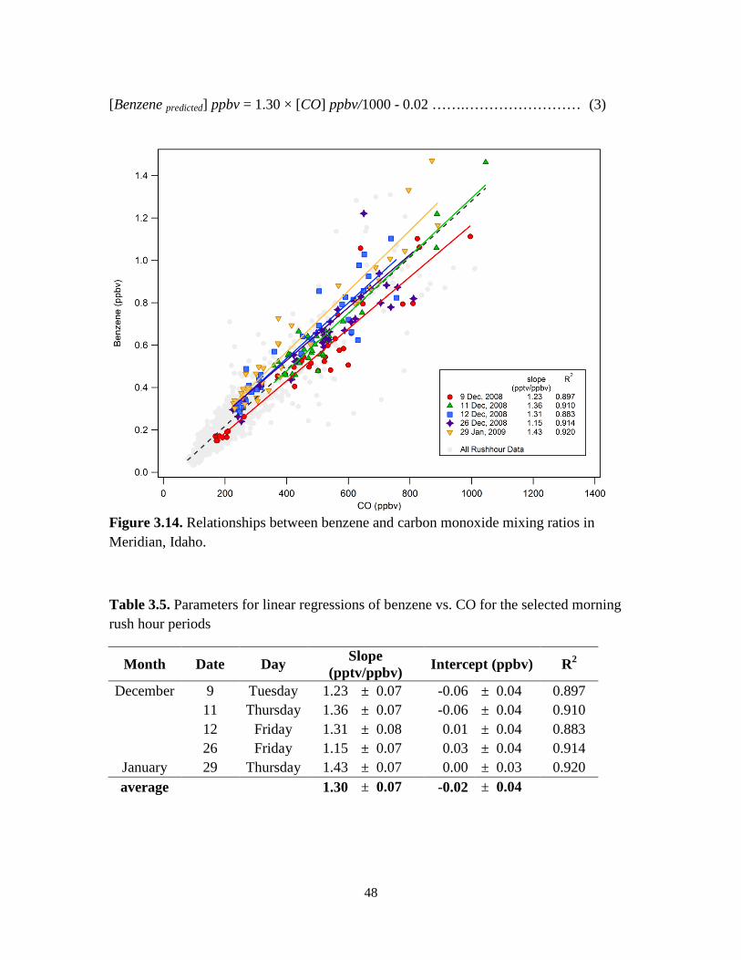
Figure 3.14. Relationships between benzene and carbon monoxide mixing ratios in

Meridian, Idaho ..................................................................................................................48

Figure 3.15. Measured and calculated (using benzene/CO ratio) benzene mixing ratios. 49

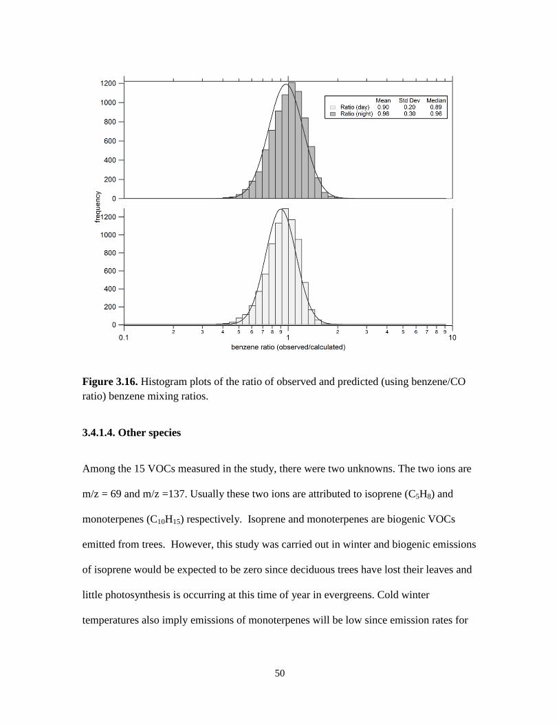
Figure 3.16. Histogram plots of the ratio of observed and predicted (using benzene/CO

ratio) of benzene mixing ratios. ........................................................................................50

xiii

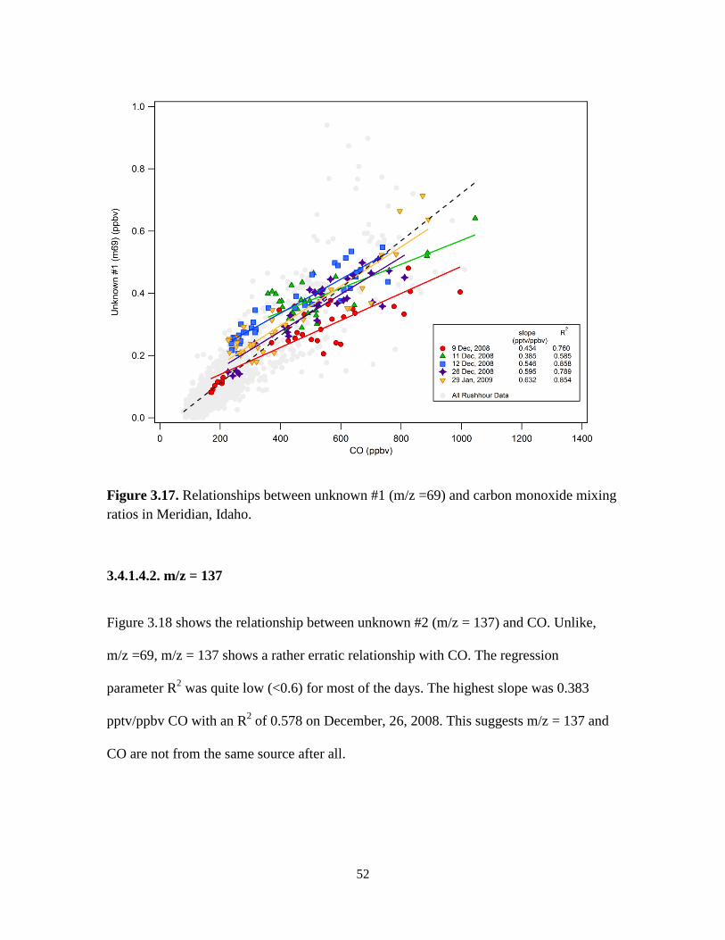
Figure 3.17. Relationships between unknown #1 (m/z =69) and carbon monoxide mixing

ratios in Meridian, Idaho. ..................................................................................................52

Figure 3.18. Relationships between unknown #2 (m/z =137) and carbon monoxide

mixing ratios in Meridian, Idaho .......................................................................................53

Figure 3.19. Relationships between aromatics and carbon monoxide mixing ratios in

Meridian, Idaho ..................................................................................................................54

Figure 3.20. Relationships between HCHO and NOx mixing ratios in Meridian, Idaho. 55

Figure 3.21. Measured and calculated (using HCHO/NOX ratio) HCHO mixing ratios. .57

Figure 3.22. Histogram plots of the ratio of observed and predicted (using HCHO/NOX

ratio) formaldehyde mixing ratios ....................................................................................58

Figure 3.23. Relationships between CH3CHO and NOx mixing ratios in Meridian, Idaho.

............................................................................................................................................59

Figure 3.24. Measured and calculated (using CH3CHO/NOX ratio) CH3CHO mixing

ratios ..................................................................................................................................60

Figure 3.25. Histogram plots of the ratio of observed and predicted (using CH3CHO/NOX

ratio) of acetaldehyde mixing ratios .................................................................................61

Figure 3.26. Relationships between benzene and NOx mixing ratios in Meridian, Idaho.

............................................................................................................................................62

Figure 3.27. Measured and calculated (using benzene/NOX ratio) benzene mixing ratios

............................................................................................................................................63

Figure 3.28. Histogram plots of the ratio of observed and predicted (using benzene/NOX

ratio) of benzene mixing ratios .........................................................................................65

Figure 3.29. Relationships between unknown #1 (m/z =69) and NOX mixing ratios in

Meridian, Idaho. ................................................................................................................66

xiv

Figure 3.30. Relationships between unknown #2 (m/z =137) and NOX mixing ratios in

Meridian, Idaho ..................................................................................................................68

Figure 3.31. Relationships between aromatics and NOX mixing ratios in Meridian, Idaho

............................................................................................................................................69

Figure 3.32. AIRPACT-3 domain. Satellite image of AIRPACT-3 domain showing major

cities and interstate highways (red lines). .........................................................................70

Figure 3.33. Comparison of HCHO/CO slopes from AIRPACT-3 model and

measurements. ...................................................................................................................72

Figure 3.34. Comparison of HCHO/NOx slopes from AIRPACT-3 model and

measurements. ...................................................................................................................73

Figure 3.35. Comparison of CH3CHO /CO slopes from AIRPACT-3 model and

measurements. ...................................................................................................................74

Figure 3.36. Comparison of CH3CHO /NOX slopes from AIRPACT-3 model and

measurements. ...................................................................................................................75

Figure 3.37. Comparison of benzene /CO slopes from AIRPACT-3 model and

measurements. ...................................................................................................................76

Figure 3.38. Comparison of benzene /NOX slopes from AIRPACT-3 model and

measurements. ...................................................................................................................77

Figure 3.39. Comparison of mono aromatics/CO slopes from AIRPACT-3 model and

measurements .....................................................................................................................78

Figure 3.40. Comparison of mono aromatics/NOX slopes from AIRPACT-3 model and

measurements .....................................................................................................................79

xv

ABBREVIATIONS

ACS American Cancer Society

AIRPACT Air Indicator Report for Public Awareness and Community Tracking

BVOC Biogenic volatile organic compounds

CAA Clean Air Act

CI Compression ignition

CMAQ Community Multi-Scale Air Quality

DHHS Department of Health and Human Services

EPA Environmental Protection Agency

HAPs Hazardous air pollutants

IARC International Agency for Research on Cancer

IDEQ Idaho Department of Environmental Quality

IUATS Integrated Urban Air Toxic Strategy

MACL Mobile atmospheric chemistry lab

MSATs Mobile Source Air Toxics

MTBE Methyl tertiary butyl ether

NAAQS National ambient air quality standards

NEI National Emission Inventory

NESHAPS National emissions standards for hazardous air pollutants

PM Particulate matters

PMSATs Priority Mobile Source Air Toxics

PTR-MS Proton transfer reaction mass spectrometer

xvi

SI Spark ignition

SOA Secondary organic aerosol

TOG Total organic gases

VMT Vehicle miles travelled

VOCs Volatile organic compounds

NOMENCLATURE

C5H8 Isoprene/ 2-methyl-1,3 butadiene

C6H6 Benzene

C10H15 Monoterpenes

CH3CHO Acetaldehyde

CH4 Methane

CO Carbon monoxide

HCHO Formaldehyde

HO Hydroxyl radical

HO2 Hydroperoxy radical

NO Nitric Oxide

NO2 Nitrogen dioxide

NO3 Nitrogen trioxide or nitrate radical

NOX Nitrogen Oxides

O3 Ozone

xvii

SO2 Sulfur dioxide

Units

ppbv parts per billion by volume

pptv parts per trillion by volume

1

CHAPTER 1: INTRODUCTION

1.1. Air toxics

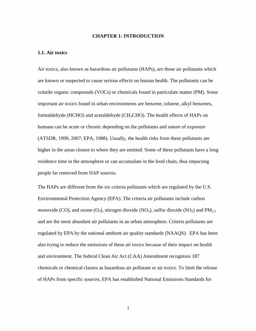
Air toxics, also known as hazardous air pollutants (HAPs), are those air pollutants which

are known or suspected to cause serious effects on human health. The pollutants can be

volatile organic compounds (VOCs) or chemicals found in particulate matter (PM). Some

important air toxics found in urban environments are benzene, toluene, alkyl benzenes,

formaldehyde (HCHO) and acetaldehyde (CH3CHO). The health effects of HAPs on

humans can be acute or chronic depending on the pollutants and nature of exposure

(ATSDR, 1999, 2007; EPA, 1988). Usually, the health risks from these pollutants are

higher in the areas closest to where they are emitted. Some of these pollutants have a long

residence time in the atmosphere or can accumulate in the food chain, thus impacting

people far removed from HAP sources.

The HAPs are different from the six criteria pollutants which are regulated by the U.S.

Environmental Protection Agency (EPA). The criteria air pollutants include carbon

monoxide (CO), and ozone (O3), nitrogen dioxide (NO2), sulfur dioxide (SO2) and PM2.5

and are the most abundant air pollutants in an urban atmosphere. Criteria pollutants are

regulated by EPA by the national ambient air quality standards (NAAQS). EPA has been

also trying to reduce the emissions of these air toxics because of their impact on health

and environment. The federal Clean Air Act (CAA) Amendment recognizes 187

chemicals or chemical classes as hazardous air pollutant or air toxics. To limit the release

of HAPs from specific sources, EPA has established National Emissions Standards for

2

Hazardous Air Pollutants (NESHAPs), according to Section 112 of the CAA (EPA,

2000b).

The EPA has also devised a strategy, known as the National Air Toxics Program: The

Integrated Urban Air Toxic Strategy (IUATS), for air toxics in urban areas by looking at

stationary, mobile, and indoor source emissions. In this strategy, EPA established a list of

33 urban HAPs which pose the greatest threats to public health in urban areas,

considering emissions from major, area and mobile sources. At the same time, the agency

compared the lists of compounds identified in the motor vehicle emission databases and

studied them with the toxic compounds listed in the Integrated Risk Information System,

IRIS. Thus, U.S. EPA identified 21 Mobile Source Air Toxics (MSATs) (EPA, 2000b),

each of which has the potential to cause serious adverse health effects as reflected in IRIS

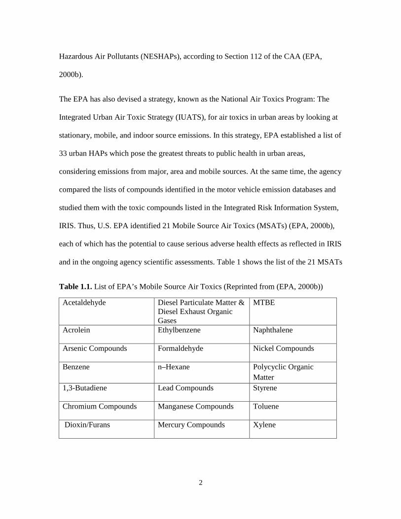
and in the ongoing agency scientific assessments. Table 1 shows the list of the 21 MSATs

Table 1.1. List of EPA’s Mobile Source Air Toxics (Reprinted from (EPA, 2000b))

Acetaldehyde Diesel Particulate Matter & Diesel Exhaust Organic Gases

MTBE

Acrolein Ethylbenzene Naphthalene

Arsenic Compounds Formaldehyde Nickel Compounds

Benzene n–Hexane Polycyclic Organic Matter

1,3-Butadiene Lead Compounds Styrene

Chromium Compounds Manganese Compounds Toluene

Dioxin/Furans Mercury Compounds Xylene

3

which include various volatile organic compounds, VOCs, and metals, as well as diesel

particulate matter, and diesel exhaust organic gases, collectively called DPM + DEOG.

Among these pollutants, six air toxics are considered to be priority mobile sources air

toxics (PMSATs) due to their higher risk to human health, according to the U.S. EPA’s

IUATS and the MSATs regulations. These are: acrolein, acetaldehyde, benzene, 1,3-

butadiene, formaldehyde, and DPM (EPA, 2000a). The focus of this thesis is on

acetaldehyde, benzene and formaldehyde.

1.2. Sources of air toxics

Most of the air toxics in the atmosphere come from anthropogenic sources as a result of

incomplete combustion of fossil fuels including roadway emissions (e.g., cars, trucks,

buses etc.), non-roadway emissions (e.g., locomotive, aviation etc.), area sources (e.g.

home heating, biomass burning etc.) and point sources (e.g., factories, refineries, power

plants, etc.). VOCs, like benzene, can be also emitted in the atmosphere through fuel

evaporation and solvent use (Borbon et al., 2004). Air toxics, like formaldehyde and

acetaldehyde, can be produced in the atmosphere photochemically from other VOCs or

biogenic volatile organic compounds (BVOCs) (Altshuller, 1993). Secondary

photochemical formation depends on various factors of the atmosphere, including

precursor concentrations and the abundance of oxidants. During summer, high emissions

of biogenic hydrocarbons (BVOCs) from plants can be a major source of secondary

formaldehyde, and lead high levels of formaldehyde during summer compared to winter

(Possanzini et al., 2002; Tago et al., 2005). Figure 1.1 shows the intricate relationship

4

between these various sources and how they contribute to toxic concentrations in the

ambient environment.

Figure 1.1. Sources of urban air toxics. The yellow boxes represent all anthropogenic and direct emission sources. The green boxes represent BVOC sources.

It is to be noted that there is no secondary production of benzene in the atmosphere. It is

directly emitted from various anthropogenic sources. The following subsections describe

the nature, health effects, sources and sinks of the three air toxics.

1.2.1. Acetaldehyde

Acetaldehyde (CH3CHO) is a carbonyl compound commonly found in the ambient

environment. It is an intermediate product of plant respiration and is formed as a product

Urban Air Toxics

Primary Sources

Mobile sources

Diesel vehicles

Gasoline vehicles

Non-mobile sources

Area sources

Point sources

Secondary Sources

Anthropogenic VOCs

Mobile sources

Non-mobile sources

Area sources

Point sources

Biogenic

Isoprene

5

of incomplete wood combustion in fireplaces and wood stoves, coffee roasting, burning

of tobacco, vehicle exhaust fumes, and coal refining and waste processing (EPA, 2000b).

Hence, many individuals are exposed to acetaldehyde by breathing ambient air.

Acetaldehyde is reasonably anticipated to be a human carcinogen based on animal studies

that have shown nasal tumors in rats and laryngeal tumors in hamsters (NTP, 2011).

Acute effects associated with exposure to acetaldehyde include irritation of the eyes, skin,

and respiratory tract.

Acetaldehyde belongs to the carbonyl/aldehyde compounds, which undergo photolysis,

reaction with OH radicals and reaction with NO3 radicals. Reactions with nitrate radical

are of minor significance (Seinfeld and Pandis, 2006), leaving the photolysis and OH

radical reaction as the major loss process, principally during summer season.

1.2.2. Benzene

Benzene is an aromatic compound commonly found in the environment. The main

sources of benzene emission in the air are emissions from burning coal and oil, benzene

waste and storage operations, motor vehicle exhaust, and evaporation from gasoline

service stations. Tobacco smoke is another source of benzene in air, particularly indoors.

Benzene accounts for 3 to 5 percent of mobile source exhaust total organic gases (TOG),

which varies depending on control technology (e.g., type of catalyst) and the levels of

benzene and aromatics in the fuel (EPA, 2000b).

The major sources of benzene exposure are tobacco smoke, automobile service stations,

exhaust from motor vehicles, and industrial emissions. Auto exhaust and industrial

6

emissions account for about 20% of the total national exposure to benzene (ATSDR,

2007).

Inhaling high levels of benzene can cause drowsiness, dizziness, rapid heart rate,

headaches, tremors, confusion, and unconsciousness. Long-term exposure to high levels

of benzene in the air can cause leukemia, particularly acute myelogenous leukemia, often

referred to as AML, which is a form of cancer that starts inside bone marrow, the soft

tissue inside bones that generate blood cells (NTP, 2011). The Department of Health and

Human Services (DHHS), the International Agency for Research on Cancer (IARC) and

the EPA, all recognizes benzene as a human carcinogen (ATSDR, 2007). Also, for

women exposed by inhalation to high levels reproductive effects have been reported; and

adverse effects on the developing fetus have been observed in animal tests (ATSDR,

2007).

The most significant degradation process for atmospheric benzene is its reaction with

atmospheric OH radicals (Seinfeld and Pandis, 2006).

1.2.3. Formaldehyde

Formaldehyde is the simplest form of aldehyde/carbonyl. It is a very common pollutant in

the atmosphere. Primary sources of HCHO are mostly anthropogenic emissions from

vehicles and biomass burning as an incomplete combustion product. Vehicle exhaust is

the dominant source of formaldehyde in urban areas (Anderson et al., 1996; Ban-Weiss et

al., 2008; EPA, 2000b; Grosjean, 1982; Grosjean et al., 2001; Grosjean et al., 2002). It is

emitted during both gasoline and diesel fuel combustion and accounts for 1 – 4% of total

7

exhaust TOG emissions, depending on control technology and fuel composition (EPA,

2000b). Primary formaldehyde emissions from mobile sources account for approximately

41% of the emissions in the 1996 National Toxics Inventory (EPA, 2000b).

Formaldehyde can be also created in the atmosphere from other VOCs through

photochemical reactions (Altshuller, 1993). These reactions depend on various factors of

the atmosphere (e.g. weather, abundance of oxidants, abundance of certain molecules,

etc.). Photo oxidation of methane (CH4) and photo oxidation of isoprene (2-methyl-1,3

butadiene (C5H8)), both can contribute to secondary production of HCHO. During

summer months, the photochemistry can contribute up to 80 – 90% of the ambient

HCHO. This contribution is low (only 30 – 40%) during winter months (Possanzini et al.,

2002; Tago et al., 2005). In summer, biogenic emissions such as isoprene dominate

compared to anthropogenic sources. Isoprene is emitted from deciduous trees and its

emission increase with elevated ambient temperature (Duane et al., 2002). Thus its photo

oxidation produces more HCHO during summer. The following reactions (R1 and R2)

are responsible for secondary production of formaldehyde from isoprene oxidation. In

these reactions, the intermediate products of the oxidation undergo unimolecular

dissociation (u.d.) and thus formaldehyde is formed.

8

The Department of Health and Human Services (DHHS) states that people can be

exposed to formaldehyde primarily from breathing indoor or outdoor air, from tobacco

smoke and from use of cosmetic products containing formaldehyde (NTP, 2011).

According to DHHS, the major sources of airborne formaldehyde exposure include

combustion sources, emissions from numerous construction and home-furnishing

products, and emission from consumer goods. Acute inhalation exposure to formaldehyde

in humans can result in respiratory symptoms, and eye, nose, and throat irritation. Other

effects seen from exposure to high levels of formaldehyde in humans are coughing,

wheezing, chest pains, and bronchitis (EPA, 1988; WHO, 1989). Chronic exposure to

formaldehyde by inhalation in humans has been associated with eye, nose, throat

irritation, and respiratory symptoms such as asthma (EPA, 1988; WHO, 1989). Based on

9

sufficient evidence of carcinogenicity from studies in humans and supporting data on

mechanisms of carcinogenesis, formaldehyde is known to be a human carcinogen (NTP,

2011).

Formaldehyde is known to be decomposed rapidly by photolysis and react with OH

radical and with oxygen radical. Its atmospheric lifetime depends on reactions with OH

and photolysis. These two reactions (R3 and R4) are important as formaldehyde

contributes to the HOx (OH + HO2) budget through its photolysis (McKeen et al., 1997;

Starn et al., 1998). Free radical sources like this can eventually contribute to tropospheric

ozone (O3) production.

HCHO + O2 + hν → 2HO2• + CO ……………………….. (R3)

HCHO + O2 + •OH → HO2• + CO + H2O ……………………….. (R4)

In a nitrogen oxide rich environment, this hydroperoxy (HO2•) radical converts into

hydroxyl radical (R5).

HO2• + NO → •OH + NO2 ………………………... (R5)

Thus, HCHO photolysis can be an important source of HOx radicals in urban

environments and have an impact on photochemical ozone production.

1.3. Air toxics in urban areas

Air toxics can pose special threats in urban areas because of the large number of people

and the variety of sources of toxic air pollutants. Individually, some of these sources may

10

not emit large amounts of toxic pollutants. However, all of these pollution sources

combined can potentially pose significant health threats, particularly to sensitive

subgroups such as children and the elderly.

Population growth in urban areas is responsible for the fast growth of mobile sources

which can lead to increased air toxics if the area does not improve the fuels or does not

use cleaner vehicle technologies. According to the American Cancer Society (ACS), the

cancer of the respiratory system, such as lung cancer, accounts for more deaths than any

other cancer in both men and women (29% and 26% respectively) ((ACS)) and exposure

to air pollution is an important risk factor. According to their fact sheet, exposure to

carcinogenic agents from environmental pollutant account for 2% of all cancer cases. the

relationship between such agents and cancer is significant, although the estimated

percentage of cancers related to environmental carcinogens is small compared to the

cancer burden from acquired factors such as tobacco smoking and poor health choices.

Even a small percentage of cancers can represent many deaths: 2% of cancer deaths in

the US in 2010 correspond to approximately 11,400 deaths. In the Pacific Northwest

region, the state of Washington was estimated to have 4,320 new respiratory cancer cases

and the state of Idaho was estimated to have 860 in 2010. For Idaho, the 2002 National-

Scale Air Toxics Assessment (NATA) model predicted the cancer risk for Ada County in

Idaho to be 32 in a million (EPA, 2010). In the 2005 NATA prediction the risk has

increased up to 43 in a million (EPA, 2011), a 34.4% increase from the previous report.

In the NATA study, Ada county ranked first in the state of Idaho for cancer risk (IDEQ,

2009).

11

Another aspect of air toxics in the urban environment is tropospheric ozone (O3).

Tropospheric ozone is a major component of photochemical smog, frequently found in

urban atmospheres. Ozone is considered a major pollutant when found in the lower

atmosphere or troposphere. It is one of the criteria pollutants regulated by EPA as

discussed in section 1.1. It is a highly reactive gas and exposure to ozone can cause

severe respiratory illnesses in human as ozone reacts with biomolecules and breaks them

down; thus affecting lung function (Devlin et al., 1997).

Tropospheric ozone is formed from the results of a reaction between atomic oxygen (O)

and molecular oxygen (O2) in the presence of a third molecule (M) (R6). The oxygen

atoms are produced primarily from photolysis of NO2 (R7). NO2 is a nitrogen oxide,

found in the atmosphere from various anthropogenic, biogenic and natural sources. The

major source of NOX (=NO+NO2) is fossil fuel combustion in high temperature. Ozone

and NO further reacts together by converting back to oxygen and NO2 and thus

completing a cycle (R8).

O + O2 + M → O3 + M ……………………………………….. (R6)

NO2 + hν → NO + O ……………………………………….. (R7)

O3 + NO → NO2 + O2 ……………………………………….. (R8)

When there are enough VOCs in the atmosphere this cycle is disrupted. As mentioned

before, VOCs undergo reactions like R3 and R4 and produce HO2• radical. Reactions like

R5 produces even more •OH radical and NO2 to create a cycle of oxidation. All these

12

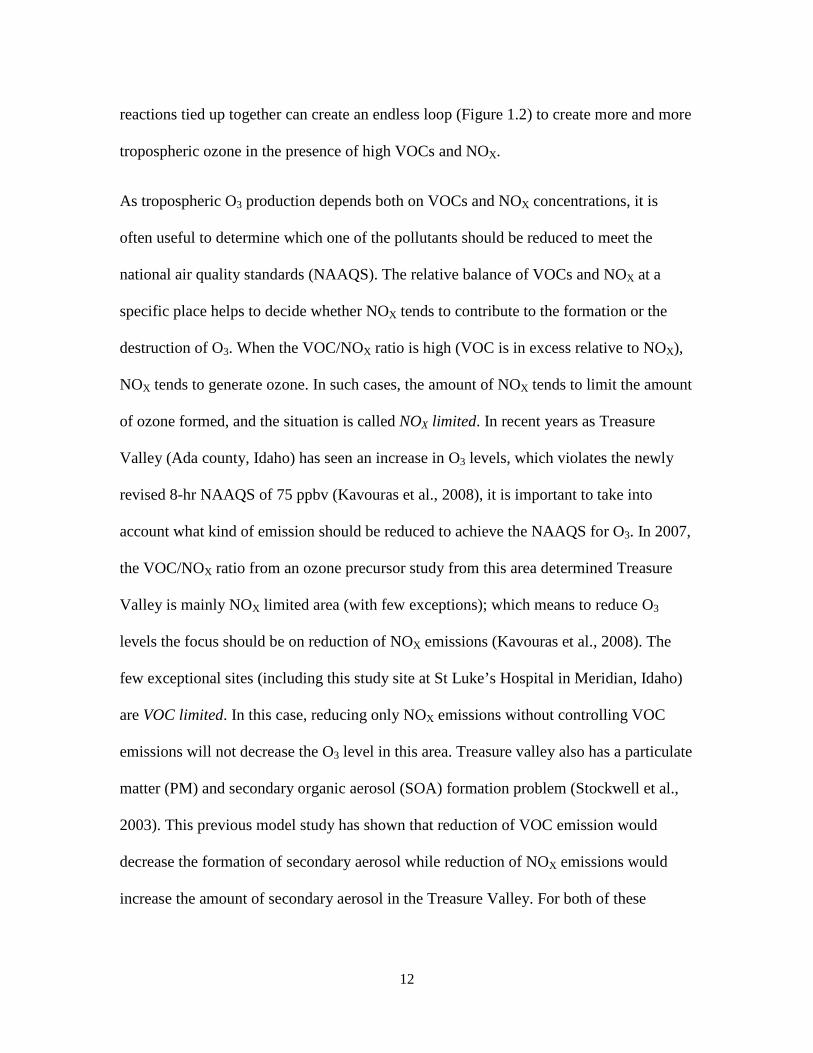
reactions tied up together can create an endless loop (Figure 1.2) to create more and more

tropospheric ozone in the presence of high VOCs and NOX.

As tropospheric O3 production depends both on VOCs and NOX concentrations, it is

often useful to determine which one of the pollutants should be reduced to meet the

national air quality standards (NAAQS). The relative balance of VOCs and NOX at a

specific place helps to decide whether NOX tends to contribute to the formation or the

destruction of O3. When the VOC/NOX ratio is high (VOC is in excess relative to NOX),

NOX tends to generate ozone. In such cases, the amount of NOX tends to limit the amount

of ozone formed, and the situation is called NOX limited. In recent years as Treasure

Valley (Ada county, Idaho) has seen an increase in O3 levels, which violates the newly

revised 8-hr NAAQS of 75 ppbv (Kavouras et al., 2008), it is important to take into

account what kind of emission should be reduced to achieve the NAAQS for O3. In 2007,

the VOC/NOX ratio from an ozone precursor study from this area determined Treasure

Valley is mainly NOX limited area (with few exceptions); which means to reduce O3

levels the focus should be on reduction of NOX emissions (Kavouras et al., 2008). The

few exceptional sites (including this study site at St Luke’s Hospital in Meridian, Idaho)

are VOC limited. In this case, reducing only NOX emissions without controlling VOC

emissions will not decrease the O3 level in this area. Treasure valley also has a particulate

matter (PM) and secondary organic aerosol (SOA) formation problem (Stockwell et al.,

2003). This previous model study has shown that reduction of VOC emission would

decrease the formation of secondary aerosol while reduction of NOX emissions would

increase the amount of secondary aerosol in the Treasure Valley. For both of these

13

Figure 1.2 Block diagram of O3 production driven by HCHO, HOX and NOX chemistry. Stable compounds are in rectangle shapes; the short lived compounds are in circles.

factors (reduction of O3 and secondary aerosol formation), VOC emission reduction is

essential, hence the knowledge about their sources becomes significant too.

14

1.4. Modeling air toxics

Modeling air toxic concentrations in urban areas sources possess special challenges

because of the various types of toxic sources. Although most HAPs are emitted directly

some are produced and destroyed through reactions in the atmosphere. These issues, as

well as receptor selection, meteorological data processing, and background concentration

selection pose significant technical challenges to the air quality modeler. Air quality

models are valuable air quality management tools. They estimate the HAPs

concentrations at many locations and the number of the locations in a model far exceeds

the number of monitors in a typical ambient monitoring network. A typical air quality

model can either use the National Emission Inventory (NEI) data or an EPA-approved

model to estimate vehicle emission. For example, an air quality forecast model for the

Northwest region AIRPACT-3 (Air Indicator Report for Public Awareness and

Community Tracking), a computerized system that runs every day and generates hourly

maps of various criteria pollutants, uses the MOBILE6.2 model mobile emissions results.

MOBILE6.2 calculates air toxics by applying a “toxics fraction” to the gram per mile

(g/mi) total organic gas (TOG) emission rate generated by the model (Heirigs et al.,

2004). However, this approach can generate a false real time assessment of the air toxic

concentrations in some regions.

Another approach to quantify air toxic emissions from vehicles is comparing it with other

vehicle emission tracers such as – carbon monoxide (CO), nitrogen oxides (NOX), VOCs

etc. and calculate their ratios (Rappengluck et al., 2010; Warneke et al., 2007). This ratio,

15

well known as an emission ratio, is a parameter that can be used to deduce the expected

emissions of a certain VOC from a vehicle exhaust tracer, thus quantifying the amount of

VOC contributed by mobile sources As CO and NO2 are criteria pollutants which are also

present in vehicle exhausts, the ambient concentration of these trace gases are readily

available from various air quality monitoring sites. To determine an emission ratio, the

standard method is to calculate the slope of the linear fit of the scatterplot of two

compounds (Warneke et al., 2007). This is a straightforward way to quantify emissions

from a certain source e.g. vehicle exhaust. Other parameters found in the regression

analysis can also help to understand the nature of the VOC emission with respect to

vehicle exhaust. The background concentration of a VOC in the absence of vehicle

exhaust can be determined from the intercept of the linear fit.

1.5. Objective

The primary objective of this study is to determine emission ratios for formaldehyde,

acetaldehyde, and benzene from roadway vehicles using data collected during the

Treasure Valley PM2.5 Study conducted in Meridian, Idaho in the winter of 2008-2009.

Emission ratios were determined by relating these air toxics concentrations to those of

CO and NOX. The correlation between the targeted VOC and CO was used to quantify

relative emission ratios from vehicles. To validate the method’s efficacy, it was compared

to model output (from MOBILE6.2) and emission inventories used by the regional

forecast model AIRPACT-3.

16

The convenience of the proposed technique is that it can be used as a predictive tool to

help air quality policy and decision-making, by using readily available ambient

monitoring data. This method can be applied to estimate the emission of any desired

VOC from vehicles or from any other major sources of that VOC.

17

CHAPTER 2: EXPERIMENTAL

The data for this thesis are from the Treasure Valley PM2.5 Study that took place in

Meridian, Idaho between December 1, 2008 and January 31, 2009. This study was

supported by the Idaho Department of Environmental Quality in an effort to better

understand PM2.5 sources in the Treasure Valley. A report on this study was prepared by

the Desert Research Institute (Kavouras et al., 2008)

2.1. Site Description

The Treasure Valley PM2.5 Study took place in Meridian, Idaho between December 1,

2008 and January 31, 2009. Meridian is a suburban area located approximately 16 km

west of the Boise city center. The measurement site was co-located with a state air

monitoring site (St. Luke’s) run by the Idaho Department of Environmental Quality

(IDEQ) on a large vacant lot behind the St. Luke’s hospital at the intersection of Eagle

Road and I-84. This has been identified as one of the busiest intersections in Idaho

(IDEQ, 2009). The St. Luke’s site EPA Air Quality Site system identifier number is

160010010. The site is part of the Speciation Trends Network (PM composition) and a

new gas phase criteria air pollutant monitoring site. The site’s coordinates are latitude

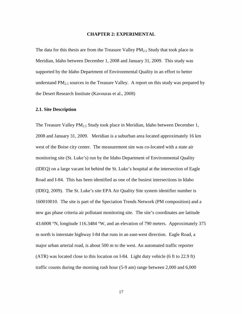
43.6008 °N, longitude 116.3484 °W, and an elevation of 790 meters. Approximately 375

m north is interstate highway I-84 that runs in an east-west direction. Eagle Road, a

major urban arterial road, is about 500 m to the west. An automated traffic reporter

(ATR) was located close to this location on I-84. Light duty vehicle (6 ft to 22.9 ft)

traffic counts during the morning rush hour (5-9 am) range between 2,000 and 6,000

18

Figure 2.1 Map of the study site in Meridian, Idaho. The blue pointer represents the approximate location of the site, NE to the St. Luke’s Hospital. Note the interstate highway (I-84) is on the south of the site. (Source: Google Maps)

vehicles, while those of heavy duty vehicles (> 22.9 feet) range between 400 and 1,000

vehicles per hour. On a daily basis about 100,000 vehicles pass the site along I-84 and

about 50,000 vehicles on Eagle Road with vehicle miles travelled (VMT) within 1 km of

the site is reported to be 381,400 (IDEQ, 2009). The site was selected by IDEQ to reflect

19

regional conditions in the valley being situated mid-point between the high population

areas of Boise in Ada County to the east and the smaller cities of Nampa and Caldwell in

Canyon County to the west. The 2010 US census reports the Ada County population to

be 392,365 and Canyon County to be 188,923. The population of Meridian is reported

to be 75,092. The monitoring site is surrounded by a mix of light industrial and

commercial spaces with limited residential development in the immediate area. The

fetches to the west northwest and southeast, the dominant air flow directions, include

mixed commercial and residential areas. Air flow through the valley is impacted by

drainage flows. The Treasure Valley slopes towards the northwest as part of the general

topography of the Snake River Plain depression. The Boise River flows through the city

of Boise and the city’s emissions get transported in stable drainage flows to the northwest

during early morning and evening. To the immediate east of Boise rise the Boise Front

Range Mountains to an elevation of over 2,300 m. The valley is frequently impacted by

severe wintertime stagnation events.

2.2. Measurements

The Laboratory for Atmospheric Research outfitted a 50 foot portable office trailer rented

for the study with a suite of instruments to measure gas phase species (O3, CO, CO2, NO,

NO2 , NOy, VOCs), particulate matter composition and size distribution, and surface

meteorological measurements. An aerosol LIDAR was also deployed to provide

boundary layer heights and aerosol optical depth. This was the first deployment of newly

acquired instrumentation for the Mobile Atmospheric Chemistry Lab (MACL).

20

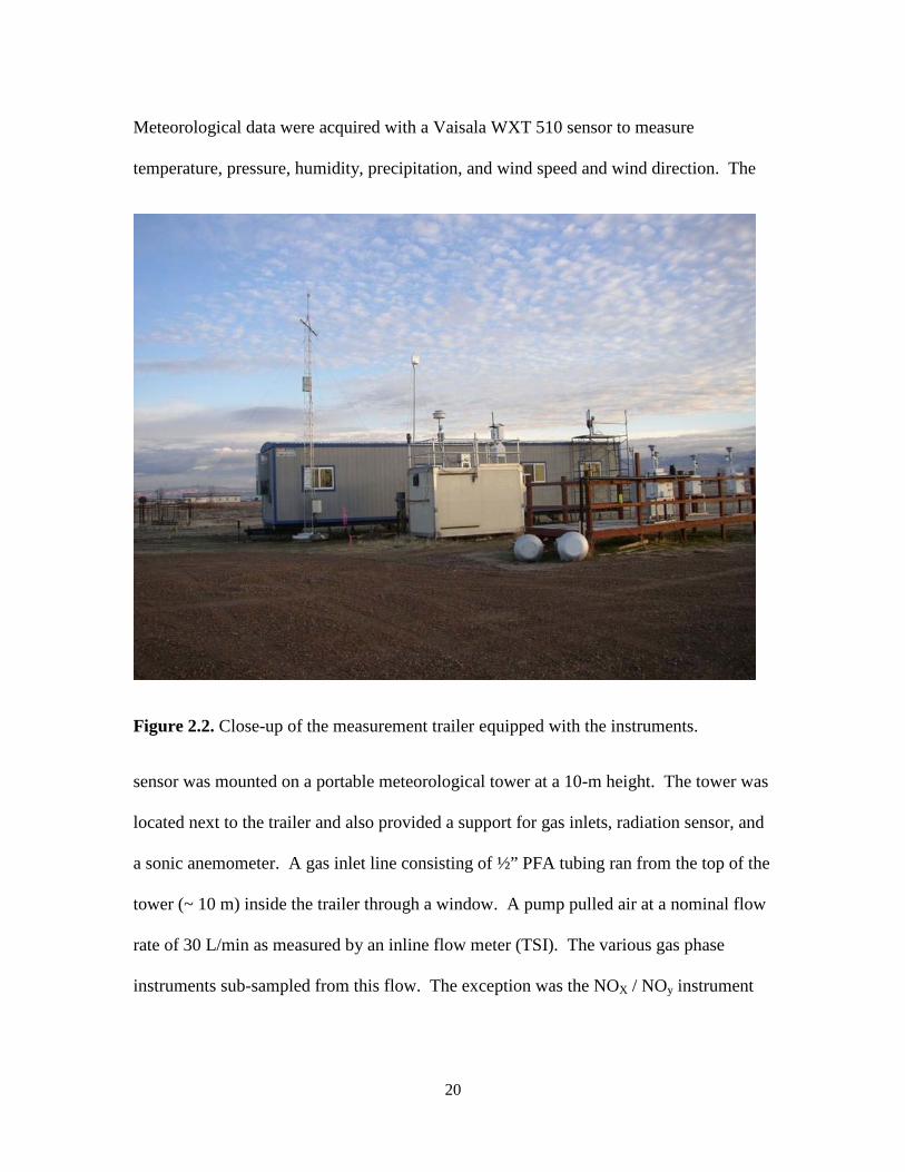
Meteorological data were acquired with a Vaisala WXT 510 sensor to measure

temperature, pressure, humidity, precipitation, and wind speed and wind direction. The

Figure 2.2. Close-up of the measurement trailer equipped with the instruments.

sensor was mounted on a portable meteorological tower at a 10-m height. The tower was

located next to the trailer and also provided a support for gas inlets, radiation sensor, and

a sonic anemometer. A gas inlet line consisting of ½” PFA tubing ran from the top of the

tower (~ 10 m) inside the trailer through a window. A pump pulled air at a nominal flow

rate of 30 L/min as measured by an inline flow meter (TSI). The various gas phase

instruments sub-sampled from this flow. The exception was the NOX / NOy instrument

21

which has its own dedicated inlet / converter box mounted on the tower at about 6-m

height.

NO, NO2, and NOy (NOxy) were measured using a two channel chemiluminescence NO

detector (Air Quality Design). NOy was measured on one channel by conversion to NO

with a molybdenum oxide catalytic converter. NO2 and NO were measured on the other

channel. NO2 was converted to NO using a blue light photolytic converter. Calibrations

were performed every 23 hours, and zeros were performed every 120 seconds. A NIST

traceable NO calibration standard of 5.03 ppmv ± 1% (Scott-Marrin Inc) was diluted in

dry zero air to provide a 25 ± 5.4% ppbv NO calibration level. Calibration of the NO2

converter efficiency was performed using gas phase titration of NO to NO2. A nitric acid

perm tube (KinTek Laboratories) was used to calibrate the conversion efficiency of

HNO3 by the molybdenum oxide catalytic converter, which remained steady at between

96 and 98% throughout the campaign. Data were recorded at 1 Hz and 2 minute averages

reported.

CO was measured with a VUV fluorescence instrument (Aerolaser GmbH). Standard

addition calibrations were performed every 4 hours using a NIST Traceable 10.01 ppmv

standard cal gas ± 1% (Scott- Marrin). The CO instrument response time was on the

order of 1 second with detection limits of ~ 10 ppbv for a 1 second integration time. The

CO data were recorded at 1 Hz and averaged to 1 minute for archiving. O3 was measured

by a Dasibi 1003 UV absorption analyzer and 1 minute averages reported for data

archiving.

22

Volatile organic compounds (VOCs) were measured with a Proton Transfer Reaction

Mass Spectrometer (PTR-MS, Ionicon Analytik GmbH). The instrument was operated at

120 Td drift field condition (2 mbar drift pressure, 60 °C drift temperature, and a drift

voltage of 535 volts). Twenty-five organic ions were monitored with dwell times ranging

from 1 to 5 seconds resulting in a 1 minute measurement cycle. The PTR-MS was

calibrated and zeroed on an automated, regular schedule using a 14 VOC component

compressed gas standard with a stated accuracy of ± 5% (Scott- Marrin, USA). The

standard was diluted to 19.8 ppbv with humid zero air produced by scrubbing ambient air

with a Pt catalyst (1% Pt on alumina spheres) at 260 °C. The sensitivity to formaldehyde

was determined in the field using an HCHO permeation device (Kintek Laboratories)

diluted with humid zero air to 40 ppbv. The PTR-MS displays a humidity dependent

sensitivity to HCHO (Jobson and McCoskey, 2010). The humidity dependence was

determined in the lab prior to the field experiment and verified with post field experiment

calibrations. The ion m/z=39 corresponding to the proton bound cluster H+(H2O)2 is

linearly proportional to ambient water vapor and allows for HCHO sensitivity to be

accurately determined.

23

CHAPTER 3: RESULTS AND DISCUSSION

3.1. Data Description

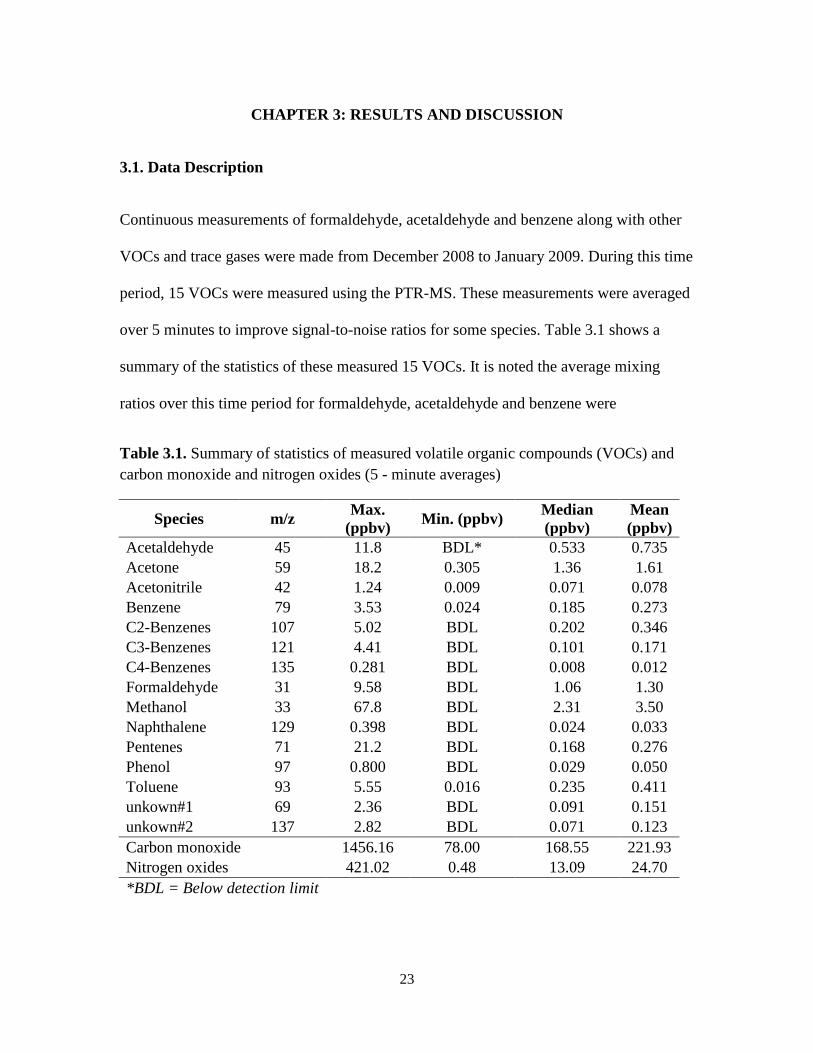
Continuous measurements of formaldehyde, acetaldehyde and benzene along with other

VOCs and trace gases were made from December 2008 to January 2009. During this time

period, 15 VOCs were measured using the PTR-MS. These measurements were averaged

over 5 minutes to improve signal-to-noise ratios for some species. Table 3.1 shows a

summary of the statistics of these measured 15 VOCs. It is noted the average mixing

ratios over this time period for formaldehyde, acetaldehyde and benzene were

Table 3.1. Summary of statistics of measured volatile organic compounds (VOCs) and carbon monoxide and nitrogen oxides (5 - minute averages)

Species m/z Max. (ppbv) Min. (ppbv) Median

(ppbv) Mean (ppbv)

Acetaldehyde 45 11.8 BDL* 0.533 0.735 Acetone 59 18.2 0.305 1.36 1.61 Acetonitrile 42 1.24 0.009 0.071 0.078 Benzene 79 3.53 0.024 0.185 0.273 C2-Benzenes 107 5.02 BDL 0.202 0.346 C3-Benzenes 121 4.41 BDL 0.101 0.171 C4-Benzenes 135 0.281 BDL 0.008 0.012 Formaldehyde 31 9.58 BDL 1.06 1.30 Methanol 33 67.8 BDL 2.31 3.50 Naphthalene 129 0.398 BDL 0.024 0.033 Pentenes 71 21.2 BDL 0.168 0.276 Phenol 97 0.800 BDL 0.029 0.050 Toluene 93 5.55 0.016 0.235 0.411 unkown#1 69 2.36 BDL 0.091 0.151 unkown#2 137 2.82 BDL 0.071 0.123 Carbon monoxide 1456.16 78.00 168.55 221.93 Nitrogen oxides 421.02 0.48 13.09 24.70 *BDL = Below detection limit

24

respectively 1.30, 0.74 and 0.27 ppbv. For formaldehyde and acetaldehyde, these mixing

ratios are consistent with the mixing ratios found in big cities during winter (Anderson et

al., 1996; Ho et al., 2002; Possanzini et al., 1996; Tago et al., 2005).

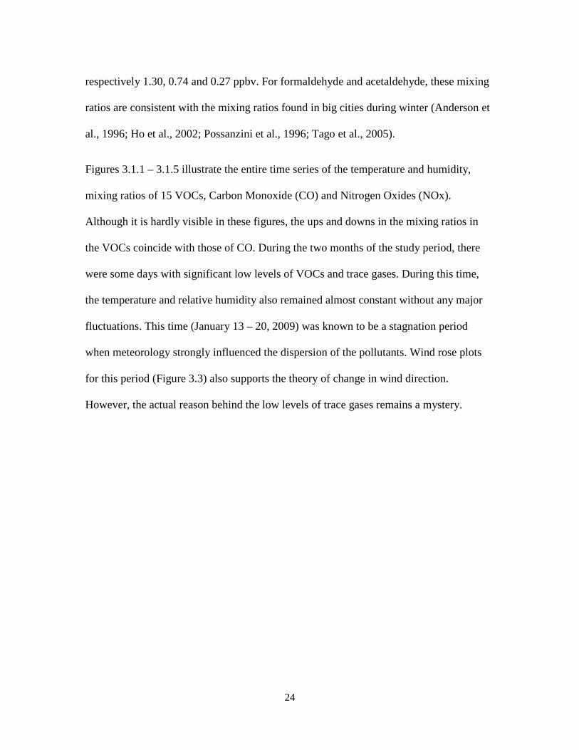
Figures 3.1.1 – 3.1.5 illustrate the entire time series of the temperature and humidity,

mixing ratios of 15 VOCs, Carbon Monoxide (CO) and Nitrogen Oxides (NOx).

Although it is hardly visible in these figures, the ups and downs in the mixing ratios in

the VOCs coincide with those of CO. During the two months of the study period, there

were some days with significant low levels of VOCs and trace gases. During this time,

the temperature and relative humidity also remained almost constant without any major

fluctuations. This time (January 13 – 20, 2009) was known to be a stagnation period

when meteorology strongly influenced the dispersion of the pollutants. Wind rose plots

for this period (Figure 3.3) also supports the theory of change in wind direction.

However, the actual reason behind the low levels of trace gases remains a mystery.

25

Figure 3.1.1 Plots of 5 - minute averaged data of temperature, relative humidity, formaldehyde (HCHO), nitrogen oxides (NOX) and carbon monoxide (CO) mixing ratios in Meridian, Idaho, from 1 December, 2008 to 31 January, 2009.

26

Figure 3.1.2 Plots of 5 - minute averaged data of acetaldehyde, acetone, acetonitrile and benzene mixing ratios in Meridian, Idaho, from 1 December, 2008 to 31 January, 2009.

27

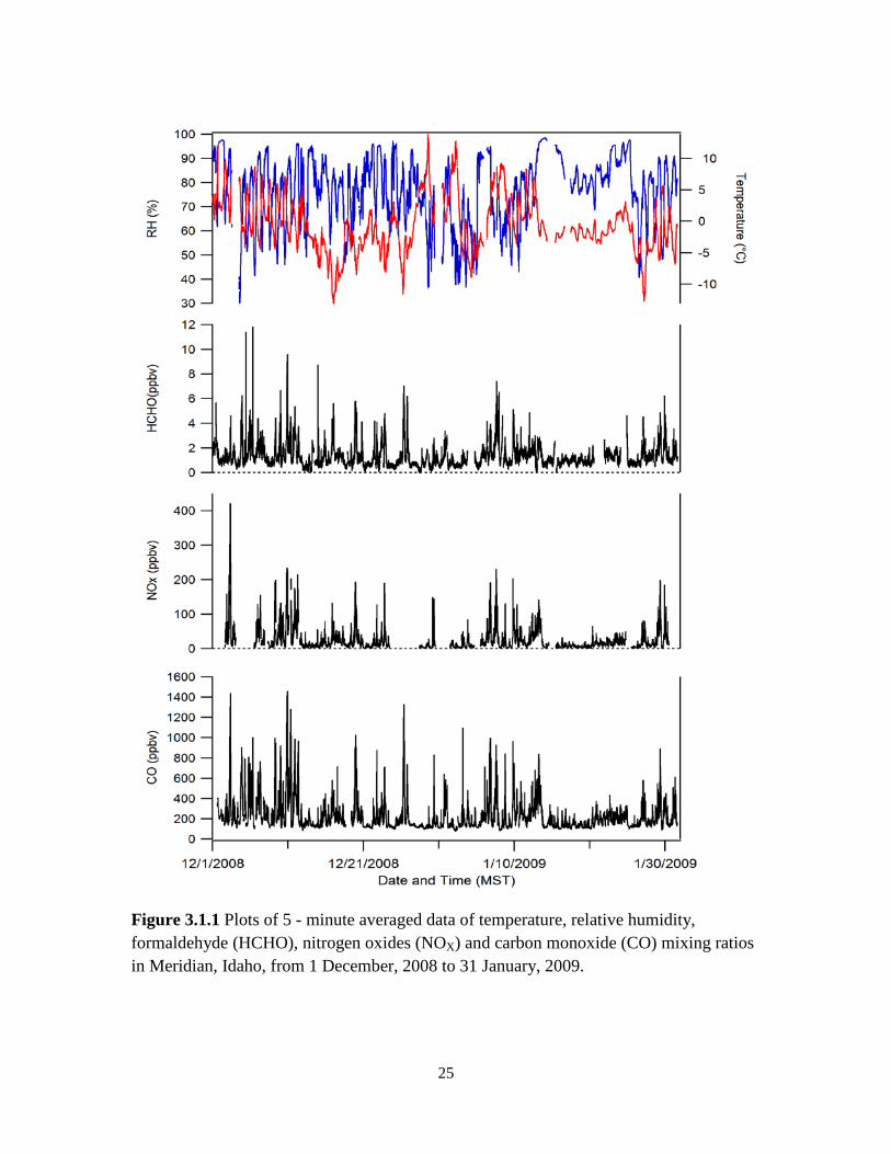
Figure 3.1.3 Plots of 5 - minute averaged data of C2-benzene, C3-benzene, C3-benzene and methanol mixing ratios in Meridian, Idaho, from 1 December, 2008 to 31 January, 2009.

28

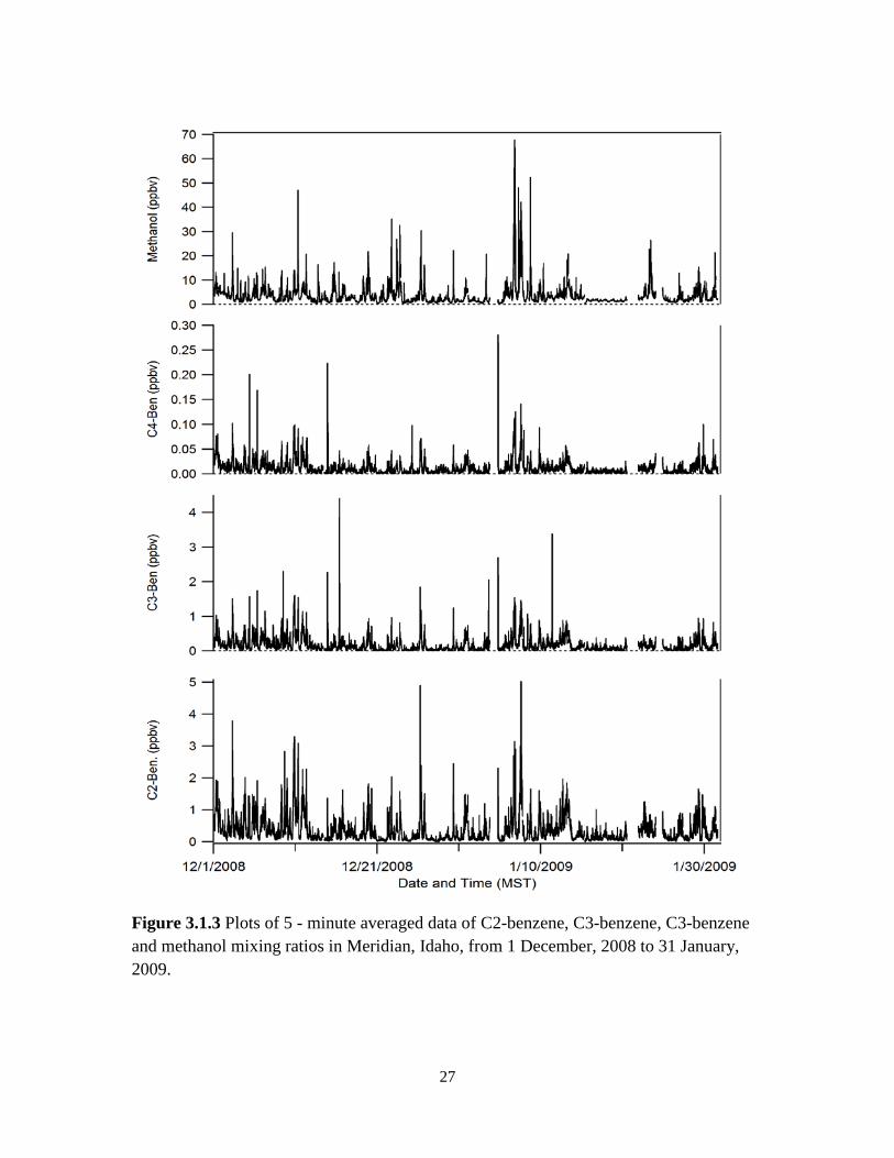
Figure 3.1.4 Plots of 5 - minute averaged data of naphthalene, pentenes, phenol and toluene mixing ratios in Meridian, Idaho, from 1 December, 2008 to 31 January, 2009.

29

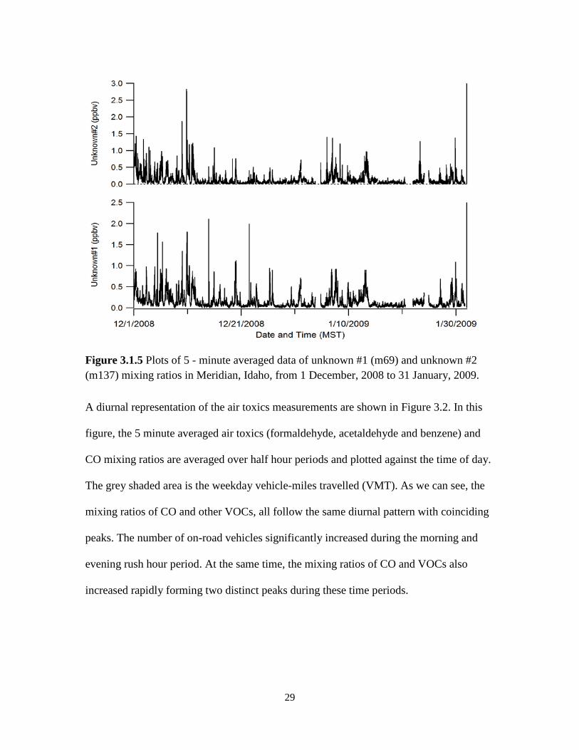
Figure 3.1.5 Plots of 5 - minute averaged data of unknown #1 (m69) and unknown #2 (m137) mixing ratios in Meridian, Idaho, from 1 December, 2008 to 31 January, 2009.

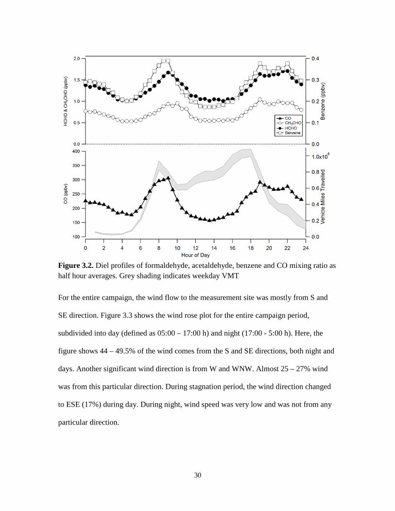
A diurnal representation of the air toxics measurements are shown in Figure 3.2. In this

figure, the 5 minute averaged air toxics (formaldehyde, acetaldehyde and benzene) and

CO mixing ratios are averaged over half hour periods and plotted against the time of day.

The grey shaded area is the weekday vehicle-miles travelled (VMT). As we can see, the

mixing ratios of CO and other VOCs, all follow the same diurnal pattern with coinciding

peaks. The number of on-road vehicles significantly increased during the morning and

evening rush hour period. At the same time, the mixing ratios of CO and VOCs also

increased rapidly forming two distinct peaks during these time periods.

30

Figure 3.2. Diel profiles of formaldehyde, acetaldehyde, benzene and CO mixing ratio as half hour averages. Grey shading indicates weekday VMT

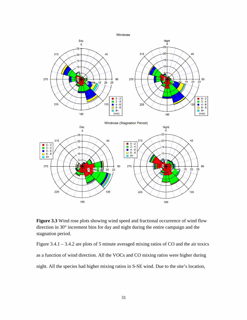
For the entire campaign, the wind flow to the measurement site was mostly from S and

SE direction. Figure 3.3 shows the wind rose plot for the entire campaign period,

subdivided into day (defined as 05:00 – 17:00 h) and night (17:00 - 5:00 h). Here, the

figure shows 44 – 49.5% of the wind comes from the S and SE directions, both night and

days. Another significant wind direction is from W and WNW. Almost 25 – 27% wind

was from this particular direction. During stagnation period, the wind direction changed

to ESE (17%) during day. During night, wind speed was very low and was not from any

particular direction.

31

Figure 3.3 Wind rose plots showing wind speed and fractional occurrence of wind flow direction in 30° increment bins for day and night during the entire campaign and the stagnation period.

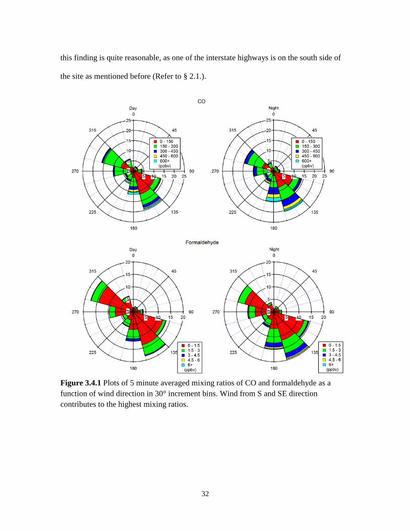
Figure 3.4.1 – 3.4.2 are plots of 5 minute averaged mixing ratios of CO and the air toxics

as a function of wind direction. All the VOCs and CO mixing ratios were higher during

night. All the species had higher mixing ratios in S-SE wind. Due to the site’s location,

32

this finding is quite reasonable, as one of the interstate highways is on the south side of

the site as mentioned before (Refer to § 2.1.).

Figure 3.4.1 Plots of 5 minute averaged mixing ratios of CO and formaldehyde as a function of wind direction in 30° increment bins. Wind from S and SE direction contributes to the highest mixing ratios.

33

Figure 3.4.2 Plots of 5 minute averaged mixing ratios of Acetaldehyde and Benzene as a function of wind direction in 30° increment bins. Wind from S and SE direction contributes to the highest mixing ratios.

34

3.2. Morning Rush hour Analysis

To analyze HCHO and its relationship to vehicle emissions, carbon monoxide (CO) was

chosen as the main vehicle emission tracer similar to previous studies (Anderson et al.,

1996; Friedfeld et al., 2002; Possanzini et al., 1996; Rappengluck et al., 2010). Carbon

monoxide can act as an excellent tracer because the main source of CO is incomplete

combustion of fossil fuel e.g. from automobiles, etc. A direct connection of atmospheric

CO mixing ratio and vehicle exhaust is found from the analysis of vehicle-miles travelled

(VMT) plots. Vehicle-miles travelled (VMT) is the total number of miles driven by all

vehicles within a given time period and geographic area. It is a useful planning tool used

by regional transportation and environmental agencies. A daily VMT plot depicts

increase of vehicles on the road during a specific time of the day. A typical day has two

significant spikes in VMT, shown in Figure 3.2, the morning rush hour period and the

evening rush hour period. Figure 3.2 also shows how atmospheric CO mixing ratio

corresponds to VMT. The plot shows CO mixing ratios follow a similar pattern as VMT

with two significant increases during the morning and evening rush hour. As discussed

before the mixing ratios of the air toxics also follow this same pattern. This suggests that

vehicle exhaust is one of the main sources of atmospheric CO and air toxics. So this gas

can be used as a valid tracer for vehicle exhaust.

Another important point to remember when discussing tracers, all vehicles does not emit

CO equally. The combustion processes of different fueled vehicles are different. For

example- the exhaust from a spark ignition (SI) vehicle will contain more CO than a

35

compression ignition (CI) vehicle. In an SI engine, the combustion process goes through

at a lower temperature than a CI engine. This lower temperature can burn the fuel

(usually gasoline) inefficiently causing more CO in the exhaust. On the other hand, a very

high temperature in the combustion chamber of a CI engine results a little CO in the

exhaust. However, the high temperature can cause more nitrogen oxides (NOX = NO

+NO2) than an SI engine. So CO might not be a useful tracer for CI or diesel engines. In

this case, NOX could be a more suitable choice.

Different type of vehicle can show different patterned VMT plot. Figure 3.5 and 3.6 show

VMT plots for gasoline and diesel fueled vehicles respectively. From the two plots it is

evident that the amount of gasoline fueled vehicles out number their diesel counterparts

by two orders of magnitude. Figure 3.5 shows that the VMT by gasoline fueled vehicles

have a pattern consisting two distinct rush hour peak. But the VMT plot (Figure 3.6) for

diesel fueled vehicles, is rather different. They do increase significantly during the

morning rush hour period, but remain high throughout the day and decreases only after

5:00 PM. This implies the emissions from these vehicles also remain consistently high.

36

Figure 3.5 Hourly vehicle miles travelled (VMT) of gasoline vehicles over a week (Source: IDEQ)

A fuel specific tracer, either for gasoline or diesel, could determine which VOCs are

emitted more from which types of fuel. One way to do this is to associate CO as a tracer

for gasoline fueled or SI vehicles. For diesel (or CI engines) one can use NOX as a tracer.

The preliminary hypothesis was benzene is emitted more from gasoline fueled vehicles,

whereas the aldehydes are emitted more from diesel vehicles.

37

Figure 3.6 Hourly vehicle miles travelled (VMT) of diesel vehicles over a week (Source:

IDEQ)

The diel profiles of the atmospheric VOCs (Figure 3.2) clearly suggest that they have

similar diurnal patterns of gasoline vehicles VMT. So our primary interest is to examine

vehicle exhaust originated from gasoline and use CO as a tracer. The VOCs were also

analyzed, using NOX as a tracer to further examine our hypothesis.

3.3. Selection criteria for morning rush hour periods

Formaldehyde and acetaldehyde can be generated photochemically in the atmosphere.

The absence of sunlight can assure there is no secondary formation of these VOCs in the

atmosphere. As the primary goal was to assess VOC emissions from vehicles, a time of

38

the day was selected when there was almost no sunlight to limit the possibility of HCHO

and CH3CHO formation from other VOCs emitted in the exhaust.

During the two winter months, the average sunrise in Meridian was after 8:00 AM. So the

morning rush hour period, defined as 5:00 AM – 8:00 AM, was chosen to analyze VOCs

and their relation to vehicle emissions. Also, the limited solar radiation during this period

contributed to limited turbulence and convective mixing in the atmosphere; so the

atmospheric mixing layer height was low and was consistent over this period.

We chose days with clear signature rush hour profiles of CO and VOCs, as illustrated in

Figure 3.2. The signature rush hour profile was defined as those periods where CO

mixing ratios increased by 200 ppbv at least. Days with no significant rush hour period or

unusual rush hour profiles, e.g. on weekends and holidays, were excluded from the

analysis. After checking these factors, five days (Table-3.2) were chosen from the 2

months of data.

39

3.4. Air Toxics Correlation Analysis for Rush Hour periods

3.4.1. Correlation with CO

3.4.1.1. Formaldehyde

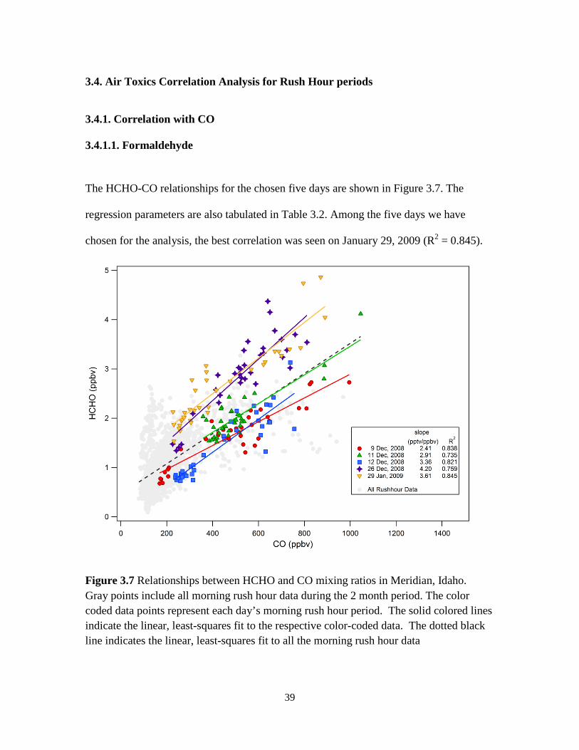
The HCHO-CO relationships for the chosen five days are shown in Figure 3.7. The

regression parameters are also tabulated in Table 3.2. Among the five days we have

chosen for the analysis, the best correlation was seen on January 29, 2009 (R2 = 0.845).

Figure 3.7 Relationships between HCHO and CO mixing ratios in Meridian, Idaho. Gray points include all morning rush hour data during the 2 month period. The color coded data points represent each day’s morning rush hour period. The solid colored lines indicate the linear, least-squares fit to the respective color-coded data. The dotted black line indicates the linear, least-squares fit to all the morning rush hour data

40

The slope was highest on December 26, 2008 (4.2 pptv HCHO/ ppbv CO) but the

regression parameter was much lower (R2 = 0.759). For the five chosen days the average

HCHO-CO slope was 3.30 ± 0.29 pptv HCHO/ppbv CO which is slightly higher than the

slope (3.0 pptv HCHO/ ppbv CO) when we include all the rush hour data for 60 days. All

of these ratios are consistent with the results from previous studies (Anderson et al.,

1996; Possanzini et al., 1996; Rappengluck et al., 2010).

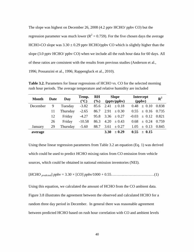
Table 3.2. Parameters for linear regressions of HCHO vs. CO for the selected morning rush hour periods. The average temperature and relative humidity are included

Month Date Day Temp. (°C)

RH (%)

Slope (pptv/ppbv)

Intercept (ppbv) R2

December 9 Tuesday -3.82 85.6 2.41 ± 0.18 0.48 ± 0.10 0.838

11 Thursday -2.65 86.7 2.91 ± 0.30 0.55 ± 0.16 0.735

12 Friday -4.27 95.8 3.36 ± 0.27 -0.03 ± 0.12 0.821

26 Friday -10.58 86.3 4.20 ± 0.43 0.68 ± 0.24 0.759 January 29 Thursday -5.60 88.7 3.61 ± 0.27 1.05 ± 0.13 0.845 average 3.30 ± 0.29 0.55 ± 0.15

Using these linear regression parameters from Table 3.2 an equation (Eq. 1) was derived

which could be used to predict HCHO mixing ratios from CO emission from vehicle

sources, which could be obtained in national emission inventories (NEI).

[HCHO predicted] ppbv = 3.30 × [CO] ppbv/1000 + 0.55……….…………………… (1)

Using this equation, we calculated the amount of HCHO from the CO ambient data.

Figure 3.8 illustrates the agreement between the observed and calculated HCHO for a

random three day period in December. In general there was reasonable agreement

between predicted HCHO based on rush hour correlation with CO and ambient levels

41

observed throughout the study period.

Figure 3.8 Measured and calculated (using HCHO/CO ratio) HCHO mixing ratios. The green points are the calculated HCHO from CO ambient data

To quantify how well the predicted formaldehyde mixing ratios correlated with the

observations, we calculated the ratio between these values. Then the ratio was plotted as a

log histogram. In the ideal case, the ratio should be equal to 1. Figure 3.9 shows the

histograms of the ratios. The ratios are subdivided into day and night time as defined

before. As we can see, for both times, the ratios are almost normally distributed. For day

and night, the average values were 0.93 ± 0.36 and 0.98 ± 0.39 respectively. This

suggests that our predicted mixing ratio are within 38% error for 64% of the time.

42

Figure 3.9 Histogram plots of the ratio of observed and predicted (using HCHO/CO ratio) formaldehyde mixing ratios.

Atmospheric formaldehyde and acetaldehyde often come from similar sources. The ratio

between these two can depict what type of source is dominant. We found that the average

formaldehyde/acetaldehyde (FA/AA) ratio was 1.50 (Table 3.4). This confirms that the

carbonyl emissions in this study were mainly from vehicles. Previous studies show,

FA/AA ratio varies from 1-2 in urban setting, dominated by vehicle emissions; it is much

higher (~10) where there is biogenic emissions (Anderson et al., 1996; Ho et al., 2002;

Possanzini et al., 1996; Viskari et al., 2000). Their relationship is shown in Figure 3.10.

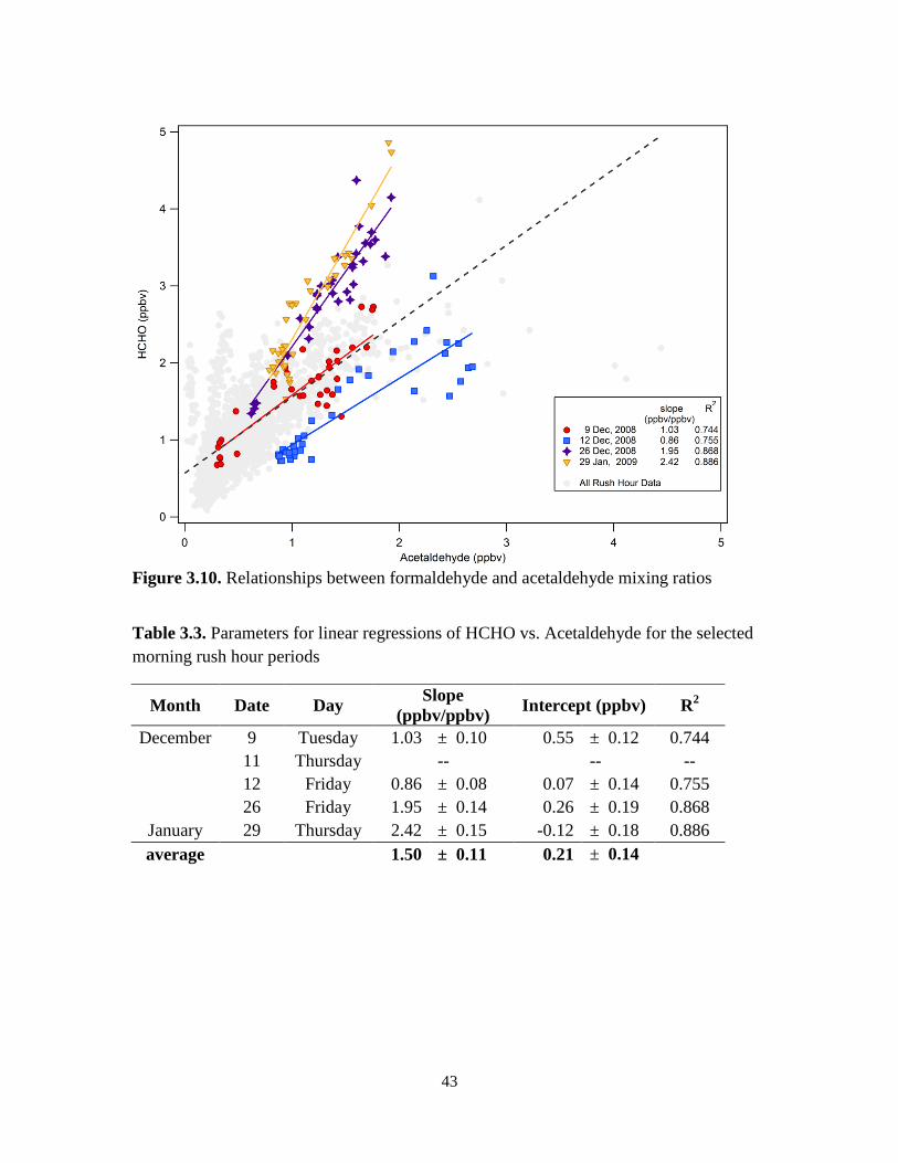
43

Figure 3.10. Relationships between formaldehyde and acetaldehyde mixing ratios

Table 3.3. Parameters for linear regressions of HCHO vs. Acetaldehyde for the selected morning rush hour periods

Month Date Day Slope (ppbv/ppbv) Intercept (ppbv) R2

December 9 Tuesday 1.03 ± 0.10 0.55 ± 0.12 0.744

11 Thursday -- -- --

12 Friday 0.86 ± 0.08 0.07 ± 0.14 0.755

26 Friday 1.95 ± 0.14 0.26 ± 0.19 0.868 January 29 Thursday 2.42 ± 0.15 -0.12 ± 0.18 0.886 average 1.50 ± 0.11 0.21 ± 0.14

44

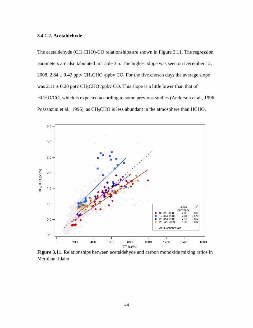
3.4.1.2. Acetaldehyde

The acetaldehyde (CH3CHO)-CO relationships are shown in Figure 3.11. The regression

parameters are also tabulated in Table 3.5. The highest slope was seen on December 12,

2008, 2.84 ± 0.42 pptv CH3CHO /ppbv CO. For the five chosen days the average slope

was 2.11 ± 0.20 pptv CH3CHO /ppbv CO. This slope is a little lower than that of

HCHO/CO, which is expected according to some previous studies (Anderson et al., 1996;

Possanzini et al., 1996), as CH3CHO is less abundant in the atmosphere than HCHO.

Figure 3.11. Relationships between acetaldehyde and carbon monoxide mixing ratios in Meridian, Idaho.

45

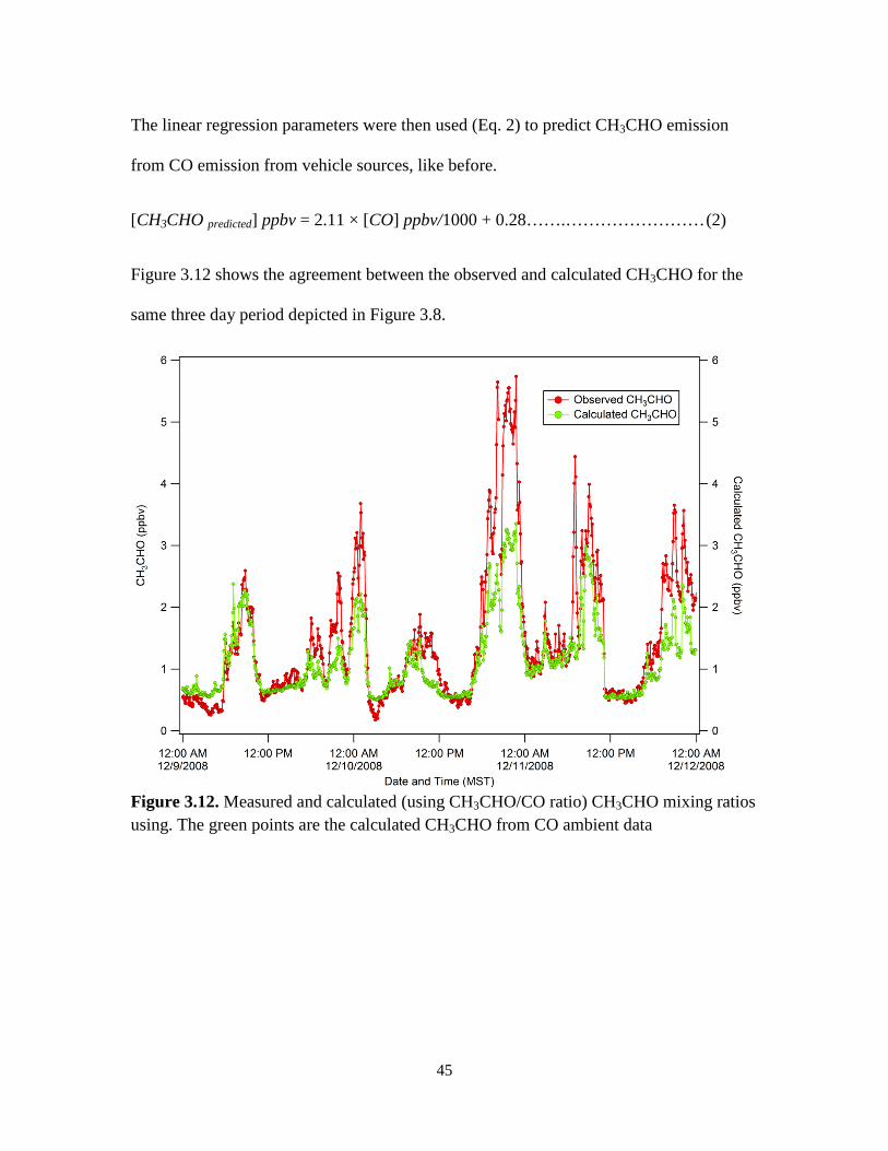
The linear regression parameters were then used (Eq. 2) to predict CH3CHO emission

from CO emission from vehicle sources, like before.

[CH3CHO predicted] ppbv = 2.11 × [CO] ppbv/1000 + 0.28…….…………………… (2)

Figure 3.12 shows the agreement between the observed and calculated CH3CHO for the

same three day period depicted in Figure 3.8.

Figure 3.12. Measured and calculated (using CH3CHO/CO ratio) CH3CHO mixing ratios using. The green points are the calculated CH3CHO from CO ambient data

46

Table 3.4. Parameters for linear regressions of Acetaldehyde vs. CO for the selected morning rush hour periods

Month Date Day Slope (pptv/ppbv) Intercept (ppbv) R2

December 9 Tuesday 2.03 ± 0.14 0.08 ± 0.08 0.854

11 Thursday -- -- --

12 Friday 2.84 ± 0.42 0.33 ± 0.19 0.579

26 Friday 2.14 ± 0.15 0.22 ± 0.09 0.862 January 29 Thursday 1.45 ± 0.08 0.50 ± 0.04 0.904 average 2.11 ± 0.20 0.28 ± 0.10

A similar check was done for the calculated acetaldehyde mixing ratios as formaldehyde.

The histograms of the ratios are shown in Figure 3.13. For acetaldehyde, the distribution

of the ratios had a positive skew. For day and night, the average values were 0.80 ± 0.40

and 0.92 ± 0.46 respectively. The median values of these distributions were 0.74 and 0.89

respectively for day and night. During day, the acetaldehyde mixing ratios were both

under and over predicted. Bur during night, the calculated acetaldehyde mixing ratios are

mostly under predicted, as we can see some higher values of ratio dominates the

distribution. The error for the predicted values for both time of the day is 43% in average.

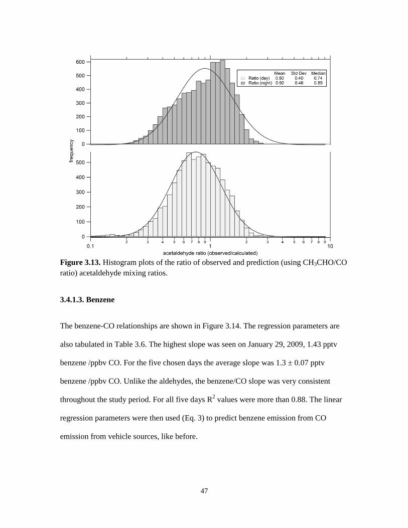
47

Figure 3.13. Histogram plots of the ratio of observed and prediction (using CH3CHO/CO ratio) acetaldehyde mixing ratios.

3.4.1.3. Benzene

The benzene-CO relationships are shown in Figure 3.14. The regression parameters are

also tabulated in Table 3.6. The highest slope was seen on January 29, 2009, 1.43 pptv

benzene /ppbv CO. For the five chosen days the average slope was 1.3 ± 0.07 pptv

benzene /ppbv CO. Unlike the aldehydes, the benzene/CO slope was very consistent

throughout the study period. For all five days R2 values were more than 0.88. The linear

regression parameters were then used (Eq. 3) to predict benzene emission from CO

emission from vehicle sources, like before.

48

[Benzene predicted] ppbv = 1.30 × [CO] ppbv/1000 - 0.02 …….…………………… (3)

Figure 3.14. Relationships between benzene and carbon monoxide mixing ratios in Meridian, Idaho.

Table 3.5. Parameters for linear regressions of benzene vs. CO for the selected morning rush hour periods

Month Date Day Slope (pptv/ppbv) Intercept (ppbv) R2

December 9 Tuesday 1.23 ± 0.07 -0.06 ± 0.04 0.897

11 Thursday 1.36 ± 0.07 -0.06 ± 0.04 0.910

12 Friday 1.31 ± 0.08 0.01 ± 0.04 0.883

26 Friday 1.15 ± 0.07 0.03 ± 0.04 0.914 January 29 Thursday 1.43 ± 0.07 0.00 ± 0.03 0.920 average 1.30 ± 0.07 -0.02 ± 0.04

49

Figure 3.15 shows the agreement between the observed and calculated benzene. Among

all the air toxics, benzene was predicted the best using the linear regression parameters

Figure 3.15. Measured and calculated (using benzene/CO ratio) benzene mixing ratios. The green points are the calculated benzene from CO ambient data

and CO emission. A check for the predicted emissions also supports this theory. For

benzene, the observation/prediction ratios show a normally distributed histogram in

Figure 3.16. The average ratios for day and night were 0.90 ± 0.20 and 0.98 ± 0.30

respectively. The calculated benzene mixing ratios for day had the narrowest distribution

among all the toxics.

50

Figure 3.16. Histogram plots of the ratio of observed and predicted (using benzene/CO ratio) benzene mixing ratios.

3.4.1.4. Other species

Among the 15 VOCs measured in the study, there were two unknowns. The two ions are

m/z = 69 and m/z =137. Usually these two ions are attributed to isoprene (C5H8) and

monoterpenes (C10H15) respectively. Isoprene and monoterpenes are biogenic VOCs

emitted from trees. However, this study was carried out in winter and biogenic emissions

of isoprene would be expected to be zero since deciduous trees have lost their leaves and

little photosynthesis is occurring at this time of year in evergreens. Cold winter

temperatures also imply emissions of monoterpenes will be low since emission rates for

51

monoterpenes are temperature dependent. These two factors lead us to a hypothesis that

these species are of non-biogenic sources and possibly ion fragments from larger organic

compounds found in exhaust. Analysis of gasoline by PTR-MS shows the presence of

an m/z = 69 ion. Analysis of diesel fuel shows the presence of an m/z = 137 ion but no

m/z = 69 ion. These ions may be useful winter time tracers for gasoline exhaust (m/z =

69) and diesel exhaust (m/z = 137) respectively. Here, two VOCs were analyzed

expecting to find fuel specific tracers for gasoline and diesel vehicle exhaust other than

CO and NOX.

3.4.1.4.1. m/z =69

We used CO as a tracer of the vehicle exhaust as before and carried out similar analysis

for unknown #1 (m/z =69). Figure 3.17 shows the relationships between m/z =69 and

CO. Although the slopes for the five chosen days, are not quite high as benzene-CO

slopes (§ 3.3.3.), m/z=69 has good correlation (R2 > 0.7) to CO for most of the days. This

suggests that m/z =69 shares common sources with CO. The highest R2 (=0.858) was

observed on December 12, 2008. The highest slope was 0.632 pptv m/z 69 /ppbv CO and

was observed on December 26, 2008 although R2 was 0.789 for that day.

52

Figure 3.17. Relationships between unknown #1 (m/z =69) and carbon monoxide mixing ratios in Meridian, Idaho.

3.4.1.4.2. m/z = 137

Figure 3.18 shows the relationship between unknown #2 (m/z = 137) and CO. Unlike,

m/z =69, m/z = 137 shows a rather erratic relationship with CO. The regression

parameter R2 was quite low (<0.6) for most of the days. The highest slope was 0.383

pptv/ppbv CO with an R2 of 0.578 on December, 26, 2008. This suggests m/z = 137 and

CO are not from the same source after all.

53

Figure 3.18. Relationships between unknown #2 (m/z =137) and carbon monoxide mixing ratios in Meridian, Idaho.

3.4.1.4.3. Aromatics

Toluene, C2-alylbenzene, and C3-alkylbenze data were summed to provide an overall

total alkyl aromatic level. Figure 3.19 shows the relationship between the total alkyl

aromatics and CO. As the figure shows these aromatics show a very strong (R2 > 0.8)

correlation to CO during the rush hour analysis for most of the days. This strong

correlation suggests that these aromatics indeed come from vehicle exhausts. The

regression parameters of this analysis are shown in Table 3.7.

54

Figure 3.19 Relationships between aromatics and carbon monoxide mixing ratios in Meridian, Idaho.

Table 3.6. Parameters for linear regressions of aromatics vs. CO for the selected morning rush hour periods

Month Date Day Slope (pptv/ppbv) Intercept (ppbv) R2

December 9 Tuesday 4.81 ± 0.27 -0.34 ± 0.14 0.900

11 Thursday 5.84 ± 0.34 -0.42 ± 0.18 0.895

12 Friday 4.44 ± 0.27 0.12 ± 0.12 0.889

26 Friday 4.35 ± 0.34 -0.03 ± 0.19 0.851 January 29 Thursday 5.55 ± 0.18 -0.13 ± 0.09 0.964 average 5.00 ± 0.28 -0.03 ± 0.15

55

3.4.2. Correlation with NOx

3.4.2.1. Formaldehyde

NOX could be used as a tracer for diesel fueled vehicles as they emit more NOX than

gasoline fueled vehicles. Regression analyses with NOX with the various VOCs can

showcase the contribution of the diesel exhausts to their emissions. Figure 3.20 shows the

relationship between HCHO and NOX Here HCHO-NOX is shown for only three days

because there was not sufficient data for NOx on 11 December and 26 December, 2008.

Figure 3.20. Relationships between HCHO and NOx mixing ratios in Meridian, Idaho.

The regression parameters for this analysis are shown in Table 3.3. As we can see, the

best correlation was seen on January 29, 2009 (R2 = 0.795) with the highest HCHO-NOX

56

ratio (14 pptv HCHO/ ppbv NOX). The average slope from the four days was 11.9 ± 1.0

pptv HCHO/ppbv NOX .

Table 3.7. Parameters for linear regressions of HCHO vs. NOx for the selected morning rush hour periods. The average temperature and relative humidity are included

Month Date Day Temp. (°C)

RH (%)

Slope (pptv/ppbv)

Intercept (ppbv) R2

December 9 Tuesday -3.82 85.60 11.3 ± 1.1 0.54 ± 0.11 0.771

11 Thursday -2.65 86.70 -- -- --

12 Friday -4.27 95.80 10.6 ± 1.4 0.53 ± 0.13 0.627

26 Friday -10.58 86.30 -- -- -- January 29 Thursday -5.60 88.70 14.0 ± 1.2 1.17 ± 0.14 0.795 average 11.9 ± 1.2 0.74 ± 0.13

Using the average linear regression parameters from the table above, an equation was

derived (Eq. 4), similar to Eq. 1. In this case, the prediction of HCHO would depend on

the ambient NOX mixing ratio.

[HCHO predicted] ppbv = 11.9 × [NOX] ppbv/1000 + 0.74……….………………… (4)

Using this equation, we calculated the amount of HCHO from the measured NOX mixing

ratio. Figure 3.21 illustrates the comparison between the observed and calculated HCHO

for the same random three day period in December as before. The predicted HCHO

mixing ratios agree reasonably with the observed levels of HCHO during the rush hour

period. However it failed to capture the high levels of HCHO during night.

57

Figure 3.21. Measured and calculated (using HCHO/NOX ratio) HCHO mixing ratios. The blue points are the calculated HCHO from NOX ambient data

The ratios between the predicted and observed levels of HCHO were plotted into

histograms as shown in Figure 3.22. The ratios were subdivided into day and night time

as defined before. For both night and day, the histograms show wider spreads than the

histograms in Figure 3.9. During both times, we see high values of the ratio, suggesting

under predicted HCHO mixing ratios. The distributions had average values 1.17 ± 0.46

and 1.27 ± 0.55. However, the nighttime histogram clearly showed a positive skew with a

median of 1.23. This suggests that the HCHO emissions were under-predicted within

55% of the error during night.

58

Figure 3.22. Histogram plots of the ratio of observed and predicted (using HCHO/NOX ratio) formaldehyde mixing ratios.

3.4.2.2. Acetaldehyde

The acetaldehyde (CH3CHO) –NOx relationships are shown in Figure 3.23. The

regression parameters are also tabulated in Table 3.5. The highest slope was seen on

December 9, 2008, 9.42 ± 0.87 pptv CH3CHO /ppbv NOx. From the regression analyses

of three days the average slope was found to be 7.99 ± 1.03 pptv CH3CHO /ppbv NOx.

59

Figure 3.23. Relationships between acetaldehyde and NOx mixing ratios in Meridian, Idaho.

The linear regression parameters were then used (Eq. 5) to predict CH3CHO emission

from NOx emission from vehicle sources, like before.

[CH3CHO predicted] ppbv = 7.99 × [NOX] ppbv/1000 + 0.50……….……………… (5)

Figure 3.24 shows the comparison between the observed and calculated CH3CHO for the

same three day period depicted in Figure 3.8.

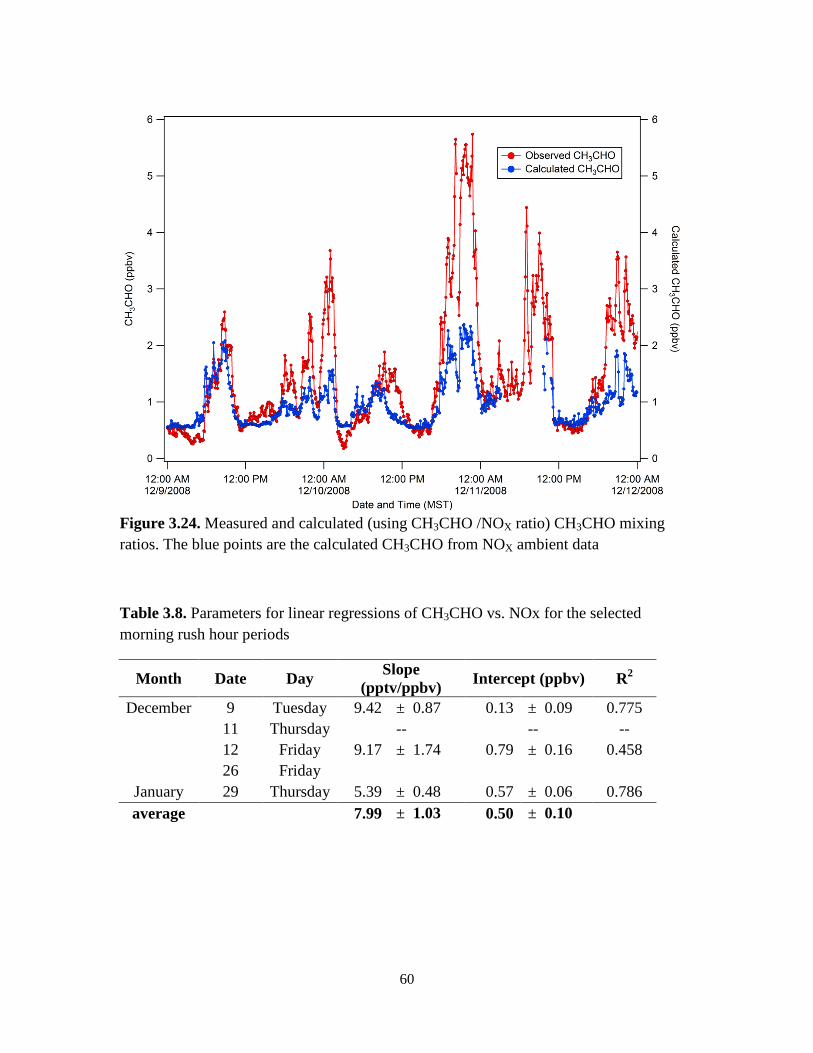
60

Figure 3.24. Measured and calculated (using CH3CHO /NOX ratio) CH3CHO mixing ratios. The blue points are the calculated CH3CHO from NOX ambient data

Table 3.8. Parameters for linear regressions of CH3CHO vs. NOx for the selected morning rush hour periods

Month Date Day Slope (pptv/ppbv) Intercept (ppbv) R2

December 9 Tuesday 9.42 ± 0.87 0.13 ± 0.09 0.775

11 Thursday -- -- --

12 Friday 9.17 ± 1.74 0.79 ± 0.16 0.458

26 Friday January 29 Thursday 5.39 ± 0.48 0.57 ± 0.06 0.786 average 7.99 ± 1.03 0.50 ± 0.10

61

The calculated CH3CHO levels were quite similar to the calculated HCHO from NOx

emissions. Both of aldehydes were under-predicted during night. However, the CH3CHO

levels were over predicted during day by equation 5. The histograms of the ratios are

shown in Figure 3.25.

Figure 3.25. Histogram plots of the ratio of observed and predicted (using CH3CHO /NOX ratio) acetaldehyde mixing ratios.

For night, the distribution of the ratios had a significant positive skew. The ratios were

mostly between 1 and 2. The average and median of this distribution were 1.04 ± 0.58

and 0.99 respectively. The day time distribution had a lesser skew than the night time

distribution. The average and median values of this distribution were 1.04 ± 0.46 and

62

0.78 respectively. These two distributions imply, predicting CH3CHO from NOX

emissions might produce false results during night.

3.4.2.3. Benzene

The benzene – NOX relationships are shown in Figure 3.26. The regression parameters

are also tabulated in Table 3.9.

Figure 3.26. Relationships between benzene and NOX mixing ratios in Meridian, Idaho.

The highest slope was seen on December 9, 2008, 5.48 pptv benzene /ppbv NOX. For the

three chosen days the average slope was 5.06 ± 0.47 pptv benzene /ppbv NOX.

63

Table 3.9. Parameters for linear regressions of benzene vs. NOX for the selected morning rush hour periods

Month Date Day Slope (pptv/ppbv) Intercept (ppbv) R2

December 9 Tuesday 5.48 ± 0.54 -0.01 ± 0.06 0.753

11 Thursday -- -- --

12 Friday 4.23 ± 0.46 0.22 ± 0.04 0.718

26 Friday -- -- -- January 29 Thursday 5.46 ± 0.41 0.05 ± 0.05 0.842 average 5.06 ± 0.47 0.09 ± 0.05

Figure 3.27 Measured and calculated (using benzene/NOX ratio) benzene mixing ratios. The blue points are the calculated benzene from NOX ambient data

The linear regression parameters were then used (Eq. 6) to predict benzene emission from

ambient NOX concentrations, like before.

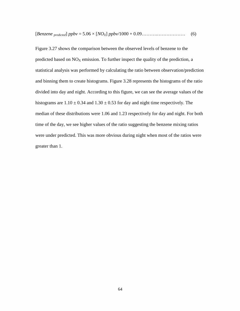
64

[Benzene predicted] ppbv = 5.06 × [NOX] ppbv/1000 + 0.09……….……………… (6)

Figure 3.27 shows the comparison between the observed levels of benzene to the

predicted based on NOX emission. To further inspect the quality of the prediction, a

statistical analysis was performed by calculating the ratio between observation/prediction

and binning them to create histograms. Figure 3.28 represents the histograms of the ratio

divided into day and night. According to this figure, we can see the average values of the

histograms are 1.10 ± 0.34 and 1.30 ± 0.53 for day and night time respectively. The

median of these distributions were 1.06 and 1.23 respectively for day and night. For both

time of the day, we see higher values of the ratio suggesting the benzene mixing ratios

were under predicted. This was more obvious during night when most of the ratios were

greater than 1.

65

Figure 3.28. Histogram plots of the ratio of observed and predicted (using benzene/NOX ratio) of benzene mixing ratios

3.4.2.4. Other species

For the two ions, m/z = 69 and m/z =137, regression analyses were done by correlating

them with NOX emissions. The hypothesis behind these analyses was that these ions were

not from biogenic sources, rather fragmented ions from larger organic compounds.

Another interest was to use these ions as a tracer for either gasoline or diesel exhaust.

Their correlations with CO (refer to § 3.4.1.4.) led us to believe, m/z = 69, usually

recognized as isoprene, shared a common source as CO. As for m/z =137, the regression

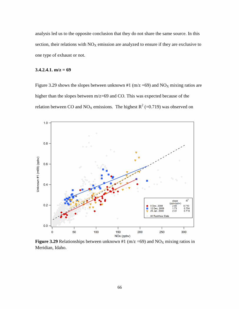
66

analysis led us to the opposite conclusion that they do not share the same source. In this

section, their relations with NOX emission are analyzed to ensure if they are exclusive to

one type of exhaust or not.

3.4.2.4.1. m/z = 69

Figure 3.29 shows the slopes between unknown #1 (m/z =69) and NOX mixing ratios are

higher than the slopes between m/z=69 and CO. This was expected because of the

relation between CO and NOX emissions. The highest R2 (=0.719) was observed on

Figure 3.29 Relationships between unknown #1 (m/z =69) and NOX mixing ratios in Meridian, Idaho.

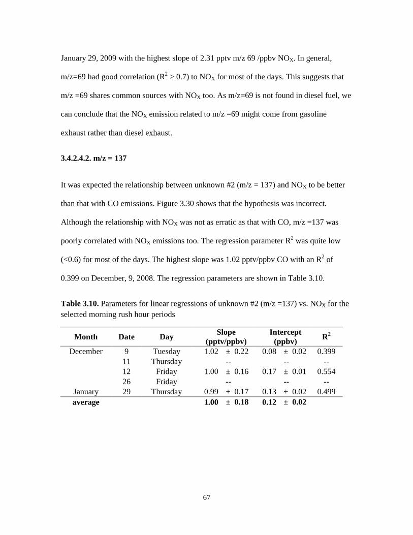
67

January 29, 2009 with the highest slope of 2.31 pptv m/z 69 /ppbv NOX. In general,

m/z=69 had good correlation (R2 > 0.7) to NOX for most of the days. This suggests that

m/z =69 shares common sources with NOX too. As m/z=69 is not found in diesel fuel, we

can conclude that the NOX emission related to m/z =69 might come from gasoline

exhaust rather than diesel exhaust.

3.4.2.4.2. m/z = 137

It was expected the relationship between unknown #2 (m/z = 137) and NOX to be better

than that with CO emissions. Figure 3.30 shows that the hypothesis was incorrect.

Although the relationship with NOX was not as erratic as that with CO, m/z =137 was

poorly correlated with NOX emissions too. The regression parameter R2 was quite low

(<0.6) for most of the days. The highest slope was 1.02 pptv/ppbv CO with an R2 of

0.399 on December, 9, 2008. The regression parameters are shown in Table 3.10.

Table 3.10. Parameters for linear regressions of unknown #2 (m/z =137) vs. NOX for the selected morning rush hour periods

Month Date Day Slope (pptv/ppbv)

Intercept (ppbv) R2

December 9 Tuesday 1.02 ± 0.22 0.08 ± 0.02 0.399

11 Thursday -- -- --

12 Friday 1.00 ± 0.16 0.17 ± 0.01 0.554

26 Friday -- -- -- January 29 Thursday 0.99 ± 0.17 0.13 ± 0.02 0.499 average 1.00 ± 0.18 0.12 ± 0.02

68

Figure 3.30 Relationships between unknown #2 (m/z =137) and NOX mixing ratios in Meridian, Idaho.

The regression parameters suggest that the m/z =137 and NOX emissions are not from the

same source. However, the intercepts were consistent and had positive values which

suggest that there were ambient m/z =137 not related to NOX emissions. Determining the

actual source of this ion is beyond the scope of this study.

3.4.2.4.3. Aromatics

Figure 3.31 shows the relationship between the total alkyl aromatics and NOX mixing

ratios. As observed here these aromatics show good (R2 > 0.7) correlation to NOX during

the rush hour analysis for most of the days. Comparing these to the previous analyses

69

with CO we can conclude that aromatics are not exclusive to CO emissions. The

regression parameters for this analysis are shown in table 3.11.

Figure 3.31 Relationships between aromatics and NOX mixing ratios in Meridian, Idaho.

Table 3.11. Parameters for linear regressions of aromatics vs. NOX for the selected morning rush hour periods

Month Date Day Slope (pptv/ppbv) Intercept (ppbv) R2

Decemeber 9 Tuesday 21.3 ± 2.1 -0.11 ± 0.23 0.745

11 Thursday -- -- --

12 Friday 14.3 ± 1.6 0.84 ± 0.15 0.720

26 Friday -- -- -- January 29 Thursday 21.1 ± 1.4 0.08 ± 0.16 0.875 average 18.9 ± 1.7 0.25 ± 0.19

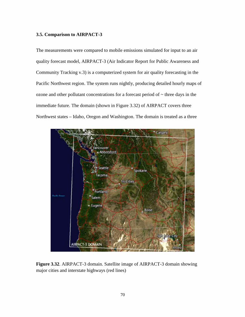
70

3.5. Comparison to AIRPACT-3

The measurements were compared to mobile emissions simulated for input to an air

quality forecast model, AIRPACT-3 (Air Indicator Report for Public Awareness and

Community Tracking v.3) is a computerized system for air quality forecasting in the

Pacific Northwest region. The system runs nightly, producing detailed hourly maps of

ozone and other pollutant concentrations for a forecast period of ~ three days in the

immediate future. The domain (shown in Figure 3.32) of AIRPACT covers three

Northwest states – Idaho, Oregon and Washington. The domain is treated as a three

Figure 3.32. AIRPACT-3 domain. Satellite image of AIRPACT-3 domain showing major cities and interstate highways (red lines)

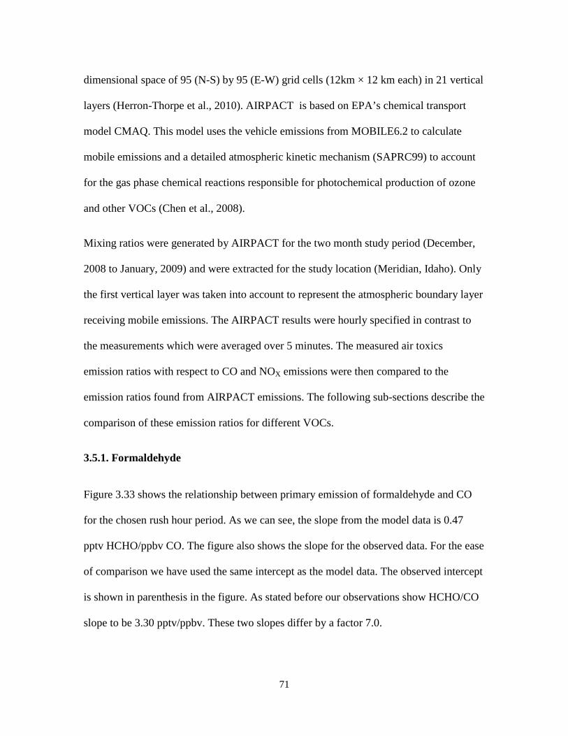
71

dimensional space of 95 (N-S) by 95 (E-W) grid cells (12km × 12 km each) in 21 vertical

layers (Herron-Thorpe et al., 2010). AIRPACT is based on EPA’s chemical transport

model CMAQ. This model uses the vehicle emissions from MOBILE6.2 to calculate

mobile emissions and a detailed atmospheric kinetic mechanism (SAPRC99) to account

for the gas phase chemical reactions responsible for photochemical production of ozone

and other VOCs (Chen et al., 2008).

Mixing ratios were generated by AIRPACT for the two month study period (December,

2008 to January, 2009) and were extracted for the study location (Meridian, Idaho). Only

the first vertical layer was taken into account to represent the atmospheric boundary layer

receiving mobile emissions. The AIRPACT results were hourly specified in contrast to

the measurements which were averaged over 5 minutes. The measured air toxics

emission ratios with respect to CO and NOX emissions were then compared to the

emission ratios found from AIRPACT emissions. The following sub-sections describe the

comparison of these emission ratios for different VOCs.

3.5.1. Formaldehyde

Figure 3.33 shows the relationship between primary emission of formaldehyde and CO

for the chosen rush hour period. As we can see, the slope from the model data is 0.47

pptv HCHO/ppbv CO. The figure also shows the slope for the observed data. For the ease

of comparison we have used the same intercept as the model data. The observed intercept

is shown in parenthesis in the figure. As stated before our observations show HCHO/CO

slope to be 3.30 pptv/ppbv. These two slopes differ by a factor 7.0.

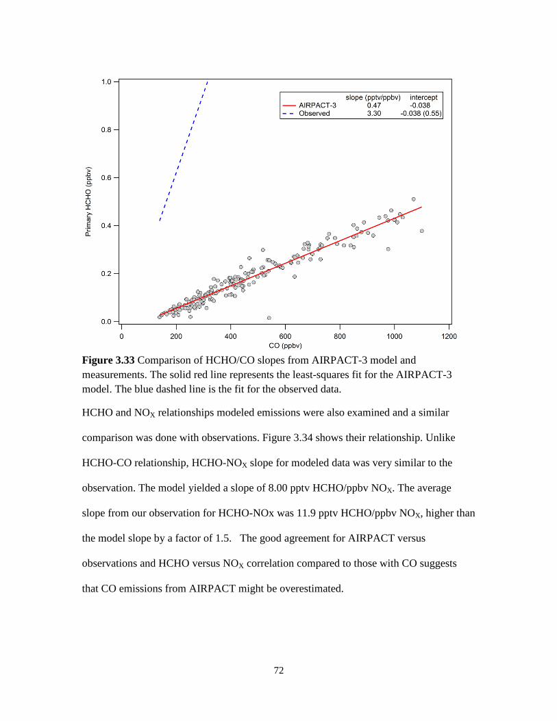
72

Figure 3.33 Comparison of HCHO/CO slopes from AIRPACT-3 model and measurements. The solid red line represents the least-squares fit for the AIRPACT-3 model. The blue dashed line is the fit for the observed data.

HCHO and NOX relationships modeled emissions were also examined and a similar

comparison was done with observations. Figure 3.34 shows their relationship. Unlike

HCHO-CO relationship, HCHO-NOX slope for modeled data was very similar to the

observation. The model yielded a slope of 8.00 pptv HCHO/ppbv NOX. The average

slope from our observation for HCHO-NOx was 11.9 pptv HCHO/ppbv NOX, higher than

the model slope by a factor of 1.5. The good agreement for AIRPACT versus

observations and HCHO versus NOX correlation compared to those with CO suggests

that CO emissions from AIRPACT might be overestimated.

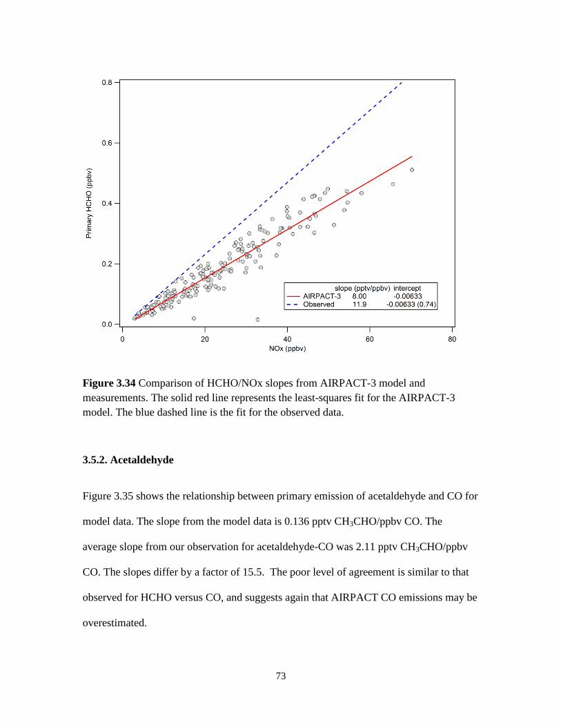
73

Figure 3.34 Comparison of HCHO/NOx slopes from AIRPACT-3 model and measurements. The solid red line represents the least-squares fit for the AIRPACT-3 model. The blue dashed line is the fit for the observed data.

3.5.2. Acetaldehyde

Figure 3.35 shows the relationship between primary emission of acetaldehyde and CO for

model data. The slope from the model data is 0.136 pptv CH3CHO/ppbv CO. The

average slope from our observation for acetaldehyde-CO was 2.11 pptv CH3CHO/ppbv

CO. The slopes differ by a factor of 15.5. The poor level of agreement is similar to that

observed for HCHO versus CO, and suggests again that AIRPACT CO emissions may be

overestimated.

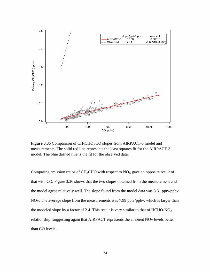
74

Figure 3.35 Comparison of CH3CHO /CO slopes from AIRPACT-3 model and measurements. The solid red line represents the least-squares fit for the AIRPACT-3 model. The blue dashed line is the fit for the observed data.

Comparing emission ratios of CH3CHO with respect to NOX gave an opposite result of

that with CO. Figure 3.36 shows that the two slopes obtained from the measurement and

the model agree relatively well. The slope found from the model data was 3.31 pptv/ppbv

NOX. The average slope from the measurements was 7.99 pptv/ppbv, which is larger than

the modeled slope by a factor of 2.4. This result is very similar to that of HCHO-NOX

relationship, suggesting again that AIRPACT represents the ambient NOX levels better

than CO levels.

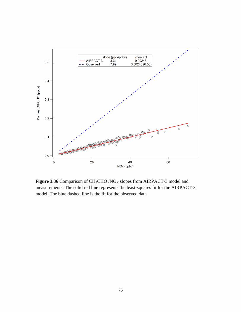
75

Figure 3.36 Comparison of CH3CHO /NOX slopes from AIRPACT-3 model and measurements. The solid red line represents the least-squares fit for the AIRPACT-3 model. The blue dashed line is the fit for the observed data.

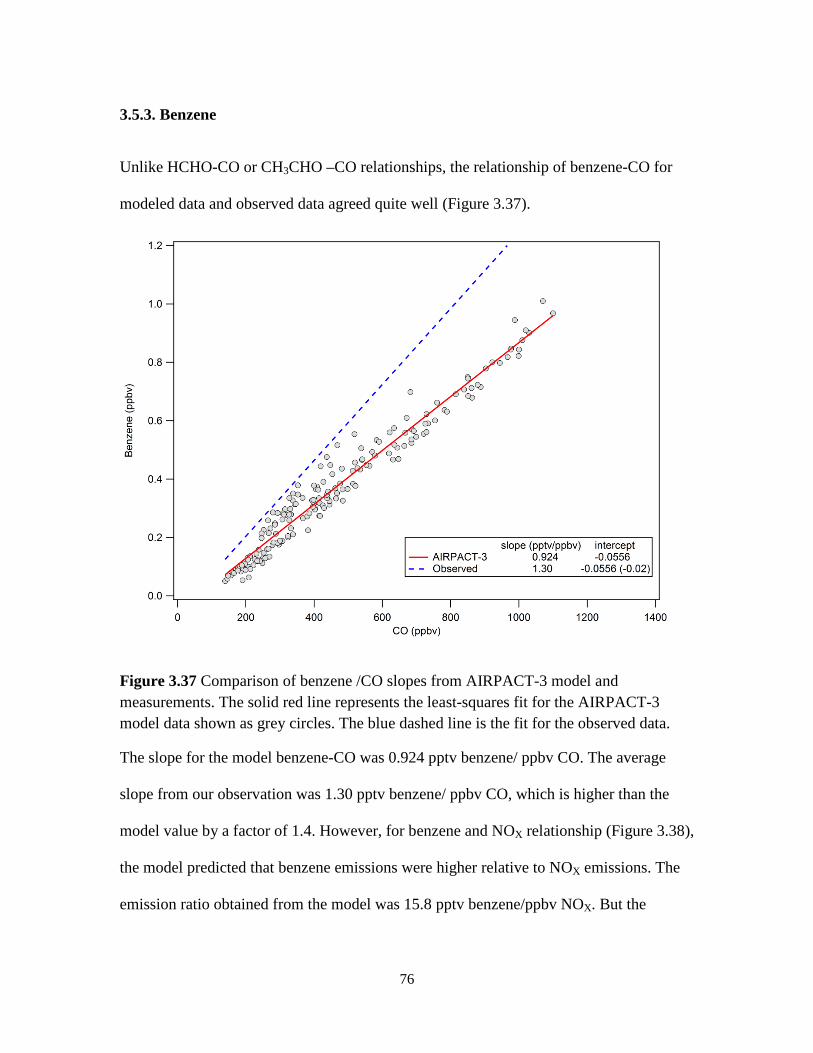
76

3.5.3. Benzene

Unlike HCHO-CO or CH3CHO –CO relationships, the relationship of benzene-CO for

modeled data and observed data agreed quite well (Figure 3.37).

Figure 3.37 Comparison of benzene /CO slopes from AIRPACT-3 model and measurements. The solid red line represents the least-squares fit for the AIRPACT-3 model data shown as grey circles. The blue dashed line is the fit for the observed data.

The slope for the model benzene-CO was 0.924 pptv benzene/ ppbv CO. The average

slope from our observation was 1.30 pptv benzene/ ppbv CO, which is higher than the

model value by a factor of 1.4. However, for benzene and NOX relationship (Figure 3.38),

the model predicted that benzene emissions were higher relative to NOX emissions. The

emission ratio obtained from the model was 15.8 pptv benzene/ppbv NOX. But the

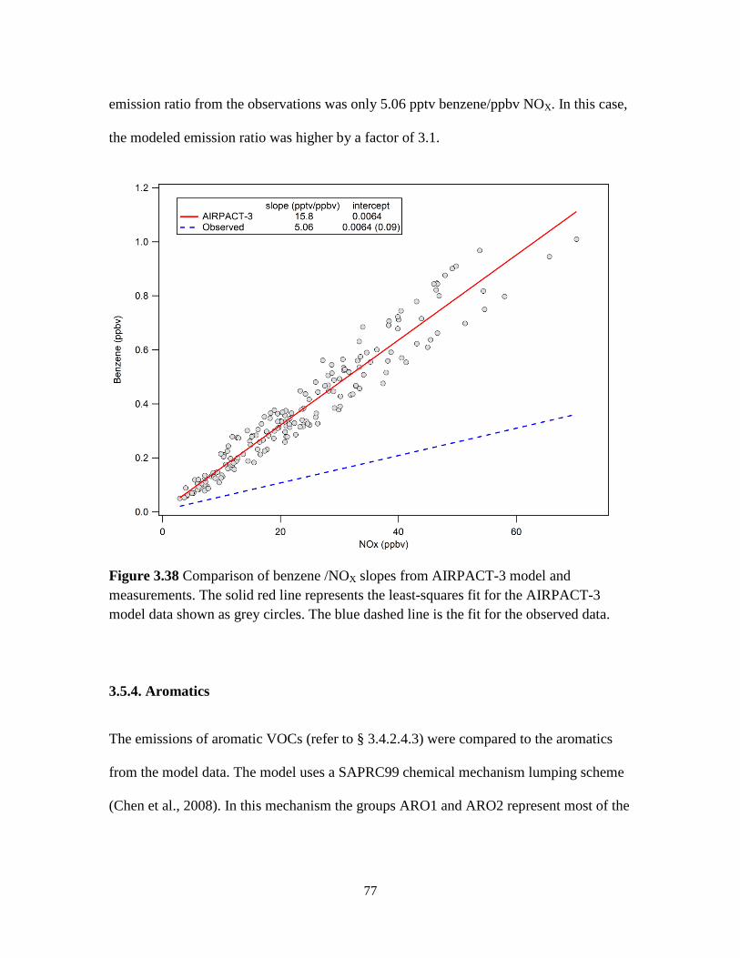
77

emission ratio from the observations was only 5.06 pptv benzene/ppbv NOX. In this case,

the modeled emission ratio was higher by a factor of 3.1.

Figure 3.38 Comparison of benzene /NOX slopes from AIRPACT-3 model and measurements. The solid red line represents the least-squares fit for the AIRPACT-3 model data shown as grey circles. The blue dashed line is the fit for the observed data.

3.5.4. Aromatics

The emissions of aromatic VOCs (refer to § 3.4.2.4.3) were compared to the aromatics

from the model data. The model uses a SAPRC99 chemical mechanism lumping scheme

(Chen et al., 2008). In this mechanism the groups ARO1 and ARO2 represent most of the

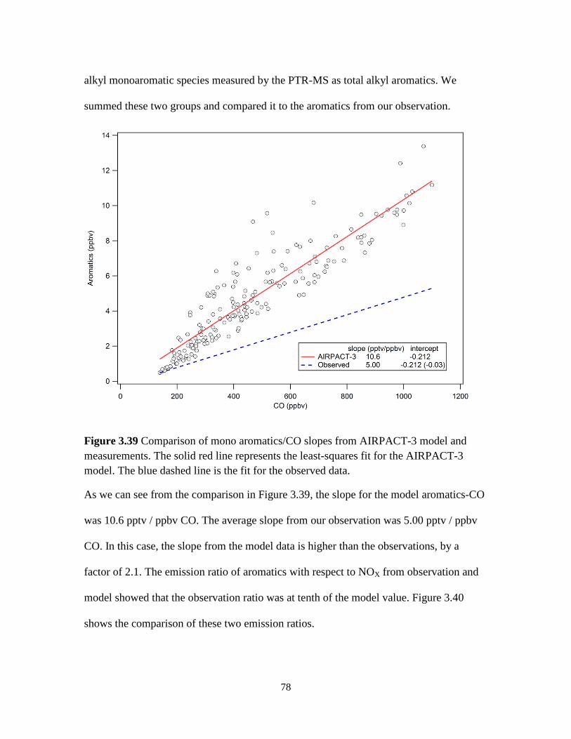
78

alkyl monoaromatic species measured by the PTR-MS as total alkyl aromatics. We

summed these two groups and compared it to the aromatics from our observation.

Figure 3.39 Comparison of mono aromatics/CO slopes from AIRPACT-3 model and measurements. The solid red line represents the least-squares fit for the AIRPACT-3 model. The blue dashed line is the fit for the observed data.

As we can see from the comparison in Figure 3.39, the slope for the model aromatics-CO

was 10.6 pptv / ppbv CO. The average slope from our observation was 5.00 pptv / ppbv

CO. In this case, the slope from the model data is higher than the observations, by a

factor of 2.1. The emission ratio of aromatics with respect to NOX from observation and

model showed that the observation ratio was at tenth of the model value. Figure 3.40

shows the comparison of these two emission ratios.

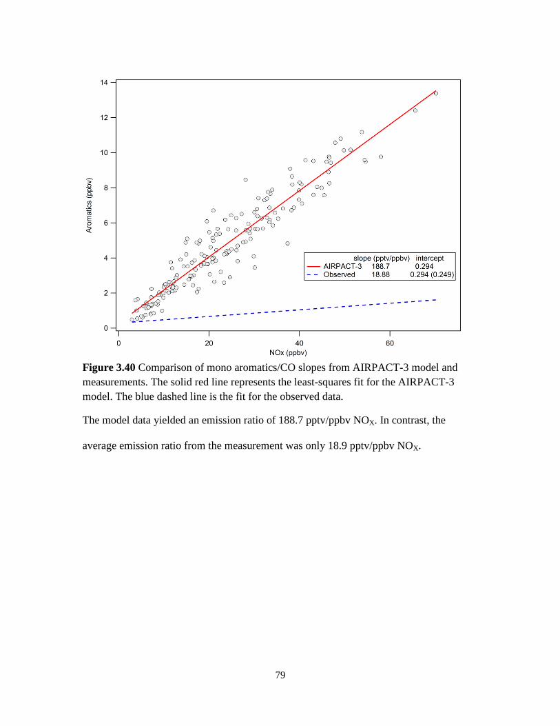
79

Figure 3.40 Comparison of mono aromatics/CO slopes from AIRPACT-3 model and measurements. The solid red line represents the least-squares fit for the AIRPACT-3 model. The blue dashed line is the fit for the observed data.

The model data yielded an emission ratio of 188.7 pptv/ppbv NOX. In contrast, the

average emission ratio from the measurement was only 18.9 pptv/ppbv NOX.

80

3.6. Summary and discussion

Emission ratios with respect to CO and NOX were calculated for priority mobile toxics,

formaldehyde, acetaldehyde and benzene, and some other VOCs of interest from

measurements in an urban environment of Meridian, Idaho during winter. Morning rush

hour during winter, in northern mid-latitudes, is an excellent time to capture the influence

of vehicle emissions on air toxics without conducting intensive tunnel studies as have

been done previously for various urban locations (Ban-Weiss et al., 2008; Grosjean et al.,

2001). We used two trace gases CO and NOX as our vehicle exhaust tracer. Our initial

hypothesis was that CO was better tracer for gasoline fueled vehicles in contrast to NOX

for diesel fueled vehicles. Unfortunately, we did not see any trend where the toxics were

more closely linked to either of the tracers. The predicted air toxic mixing ratios from

emission ratios prove that CO did better than NOX as a vehicle exhaust tracer in general.

The reasons behind the poor performance of NOX as a tracer, are related to the chemistry

of these trace gases. NOX is highly reactive. It can photolyze in the atmosphere in the

presence of sunlight. It can also be removed from the atmosphere through various

processes, especially at night. On the contrary CO has a longer atmospheric lifetime and

it is conserved throughout the day. These factors make CO a more reliable vehicle

exhaust tracer than NOX.

Emission ratios were also calculated from modeled data generated by AIRPACT. These

were compared with the measured emission ratios. According to our analyses, the

emission ratios were comparable between aldehyde –NOX and benzene-CO relationships.

81

However, the modeled ratios for aldehyde-CO relationships were significantly lower than

measured values. The lower slopes from the modeled output could be a result of

underestimating primary aldehydes (mainly HCHO) or overestimating CO in the

emission inventories.

Research conducted by Air Improvement Resource on the emission inventory model

MOBILE6.2, suggests the simulator over predicts CO emissions at colder temperatures

for some types of vehicles (Air Improvement Resource, 2005). One possible reason is

that MOBILE6.2 is unable to capture the nature of CO emissions. Recently, EPA has

developed a new mobile emission predictor known as MObile Vehicle Emission

Simulator (MOVES). Comparison between these two models (MOBILE 6.2 and

MOVES) reveals that the 80% of the wintertime ambient CO emissions come from

startup (cold start) of the vehicles. As MOBILE 6.2 cannot separate these two factors (on-

road vs. off network vehicles), it can predict higher emissions from on-road vehicles

which might not be emitting the same level of CO. This report also discusses that

MOBILE6.2 neglects the effect of vehicle fleet age on CO emissions. The prediction of

CO is reliable for vehicle fleet before the year 2000. But for the subsequent years it over-

predicts CO emissions as these vehicles are less sensitive to temperature, hence CO

emission due to cold start is significantly reduced.

Another weak point about the MOBILE6.2 model is that the air toxic emissions are

predicted through toxic fraction approach. In this approach, a toxic ratio is applies to the

total organic gas (TOG) emission rate to get the toxic emission factor. These ratios and

82

factors depend on various properties of the vehicle (type, catalytic technology used, fuel

type and characteristics, etc.). However, on an evaluation report of this model, it is

further revealed the toxic-TOG ratios for all vehicles since 1981, are calculated by a

complex model relationship which is based on emissions data prior to mid-1990s model

years (Heirigs et al., 2004). Since 1994 there has been more stringent emission standard

which are implemented for newer vehicles. These facts can greatly influence the VOC

emissions from the model itself.

Table 3.12 summarizes the emission ratios of the three air toxics with respect to CO and

NOX found in this study.

Table 3.12. Emission ratios of VOCs with respect to CO and NOX for Meridian, Idaho from measurements and from AIRPACT-3

Compounds ERmeasured (pptv/ppbv CO)

ERAIRPACT (pptv/ppbv CO)

ERmeasured (pptv/ppbv NOX)

ERAIRPACT (pptv/ppbv NOX)

acetaldehyde 2.11 0.136 7.99 3.31 aromatics 5.00 10.6 18.9 188.7 benzene 1.30 0.92 5.06 15.8 formaldehyde 3.30 0.47 11.9 8.00 unknown #1 (m/z 69) 0.519 -- 2.03 --

unknown #2 (m/z 137) 0.195 -- 1.00 --

The comparable results between the measured emission ratios and the ones from

MOBILE6.2, for NOX, suggest that the prediction of NOX emission from the model is

correct. Using this finding along with the calculated emission ratios, we can correct the

emissions of these air toxics in the model. In this case, the mixing ratios of formaldehyde,

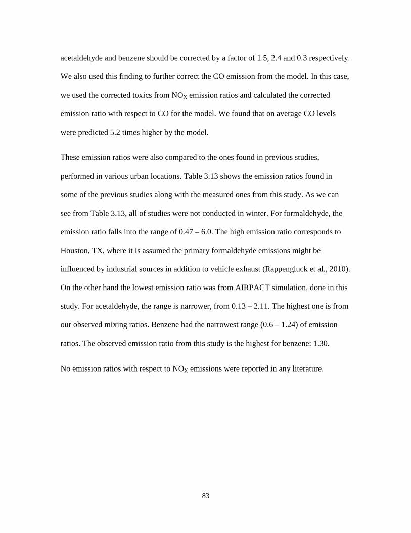
83

acetaldehyde and benzene should be corrected by a factor of 1.5, 2.4 and 0.3 respectively.

We also used this finding to further correct the CO emission from the model. In this case,

we used the corrected toxics from NOX emission ratios and calculated the corrected

emission ratio with respect to CO for the model. We found that on average CO levels

were predicted 5.2 times higher by the model.

These emission ratios were also compared to the ones found in previous studies,

performed in various urban locations. Table 3.13 shows the emission ratios found in

some of the previous studies along with the measured ones from this study. As we can

see from Table 3.13, all of studies were not conducted in winter. For formaldehyde, the

emission ratio falls into the range of 0.47 – 6.0. The high emission ratio corresponds to

Houston, TX, where it is assumed the primary formaldehyde emissions might be

influenced by industrial sources in addition to vehicle exhaust (Rappengluck et al., 2010).

On the other hand the lowest emission ratio was from AIRPACT simulation, done in this

study. For acetaldehyde, the range is narrower, from 0.13 – 2.11. The highest one is from

our observed mixing ratios. Benzene had the narrowest range (0.6 – 1.24) of emission

ratios. The observed emission ratio from this study is the highest for benzene: 1.30.

No emission ratios with respect to NOX emissions were reported in any literature.

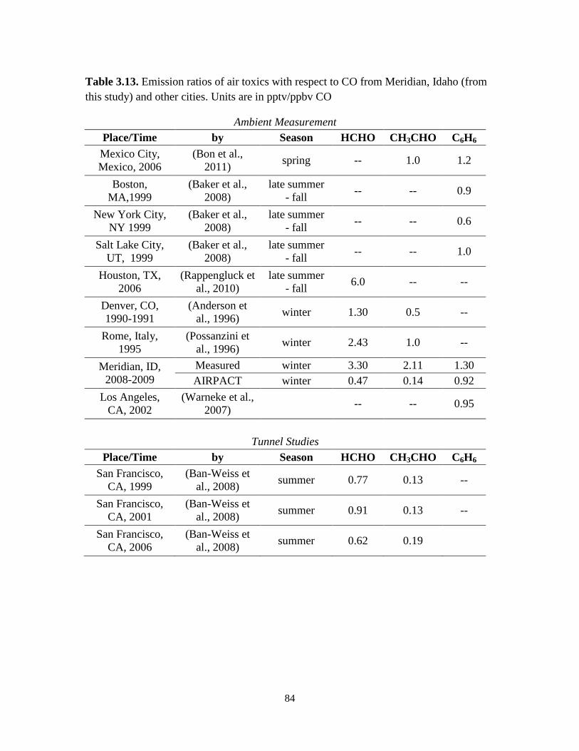
84

Table 3.13. Emission ratios of air toxics with respect to CO from Meridian, Idaho (from this study) and other cities. Units are in pptv/ppbv CO

Ambient Measurement Place/Time by Season HCHO CH3CHO C6H6 Mexico City, Mexico, 2006

(Bon et al., 2011) spring -- 1.0 1.2

Boston, MA,1999

(Baker et al., 2008)

late summer - fall -- -- 0.9

New York City, NY 1999

(Baker et al., 2008)

late summer - fall -- -- 0.6

Salt Lake City, UT, 1999

(Baker et al., 2008)

late summer - fall -- -- 1.0

Houston, TX, 2006

(Rappengluck et al., 2010)

late summer - fall 6.0 -- --

Denver, CO, 1990-1991

(Anderson et al., 1996) winter 1.30 0.5 --

Rome, Italy, 1995

(Possanzini et al., 1996) winter 2.43 1.0 --

Meridian, ID, 2008-2009

Measured winter 3.30 2.11 1.30 AIRPACT winter 0.47 0.14 0.92

Los Angeles, CA, 2002

(Warneke et al., 2007)

-- -- 0.95

Tunnel Studies

Place/Time by Season HCHO CH3CHO C6H6 San Francisco,

CA, 1999 (Ban-Weiss et

al., 2008) summer 0.77 0.13 --

San Francisco, CA, 2001

(Ban-Weiss et al., 2008) summer 0.91 0.13 --

San Francisco, CA, 2006

(Ban-Weiss et al., 2008) summer 0.62 0.19

85

CHAPTER 4: CONCLUSION

The motivation for this study was to develop a better understanding of air toxics from

mobile sources. The US EPA has labeled six air toxics to be the most hazardous to

human health, including formaldehyde, acetaldehyde and benzene, and all of them are

mainly emitted by vehicles when low temperatures inhibit biogenic emissions. This

study, conducted in Meridian, Idaho during two winter months, has given us an

opportunity to observe the relationships between these toxics and well known vehicle

exhaust tracer such as CO and NOX in urban environment. The emission ratios of these

toxics were calculated from the slope of the linear fit of scatter plots between two

compounds. We found that the emission ratios for HCHO with respect to CO and NOX

respectively to be 3.30 ± 0.29 pptv/ppbv and 11.9 ± 1.2 pptv/ppbv. As expected, the

emission ratios for acetaldehyde were a little lower, 2.11 ± 0.20 pptv/ppbv CO and 7.99 ±

1.03 pptv/ppbv NOX. Emission ratios for benzene were 1.30 ± 0.07 pptv/ppbv CO and

5.06 ± 0.47 pptv/ppbv NOX. Although there were a few studies where the relationship of

air toxics and vehicle exhaust is examined, these emission ratios were found to be in the

range of results from previous studies that were done in various cities across the globe.

Air toxics can pose a special threat in urban areas by affecting the health millions of

people. Some of these air toxics like aldehydes play an important role in atmospheric

chemistry by contributing to radical budget of a certain area. For example - formaldehyde

can also contribute to formation of ground level ozone, which is a criteria pollutant that

can cause respiratory illnesses in human. US EPA has been trying to regulate these air

86

toxics by implementing hazardous pollutant control standards (NESHAPS) where

maximum achievable control strategies are often applied to reduce the emission of these

toxics. Estimating toxics from various sources is an important step in this process. For

this purpose, EPA can rely on emission predictor models e.g. MOBILE 6.2. This

particular model was developed a long time ago and relies on outdated information on

vehicle emissions. This can mislead the current situation of certain pollutant by either

over-predicting or under-predicting some of the pollutants.

This study also compared the found emission ratios to modeled emission ratios.

AIRPACT-3 is a regional air quality forecast system for the Northwestern region of the

US. This system predicts direct emissions of acetaldehyde, benzene and formaldehyde

from vehicle source along with CO and NOX emissions. The emission ratios were

calculated by a method similar to that used for the measurements. Measured emission

ratios of aldehydes-NOX and benzene - CO compared well to the modeled data. However,

the aldehyde – CO relationship of the model resulted in emission ratios significantly

lower than those measured, by a factor of 7 - 15. This implies that the emission factor

model (MOBILE6.2) predicts erroneous emissions for the aldehydes and CO from

vehicle exhausts. Previous evaluations and criticisms of MOBILE6.2 suggest that this

error could be a result of the model’s dependence on outdated information on vehicle

emissions. Most of the algorithms developed for this model heavily rely on vehicle fleet

from mid-1990s. As technology for reduction of hydrocarbon emissions have been

deployed over the past decade, new vehicles produce lower VOCs and CO emissions.

The wide range in formaldehyde – CO emission ratios (refer to § 3.6 and Table 3.13)

87

observed in different studies suggest that the emission rates and ratios of some of these

VOCs (formaldehyde, acetaldehyde and benzene) are not well understood and

demonstrate a crucial need to incorporate these factors in future models.

The method used in this study to calculate the emission ratios of the desired VOCs was

developed through similar approaches following previous studies. The simplicity of this

method makes it a great tool to get a snapshot of air quality at a local scale. Levels of

VOCs can be measured by using the emission ratios and ambient mixing ratios of CO or

NOX available from air quality monitoring network. This can also be used as an

evaluation tool for air quality models. The emission ratios could guide modelers to see if

any of the pollutants are either under or over predicted. Comparing the emission ratios

found in this study, for NOX, to the ones from MOBILE6.2, suggest that the CO

emissions were over predicted by the model by a factor of 5.2.

One of the limitations of this analysis technique is that it was used for a very specific

time. Emission ratios found this way might not be suitable for other timeframes. During

summer months, the ambient concentration of some of the air toxics, e.g. –formaldehyde,

highly depend on their photochemical production in the atmosphere. As the study was

conducted during winter, we simply assumed this factor to be negligible as the morning

rush hour period was before sunrise. Also during summer, morning rush hour period is

not absent of sunlight and one cannot neglect the factor of photochemistry during that

period. Calculations of emission ratios during hotter months need to consider the

photochemical factor, which can be rather complicated.

88

There are several scopes to improve the analysis and calculation methods even further.

Here is a short list of recommendations for addressing certain points in future.

i. As mentioned above, the emission ratios might have the same seasonal

variability as of the air toxic itself. This could be further investigated by

conducting a long term study over several months (or years) for a certain

region.

ii. In this study, calculating emission ratios with respect to CO and NOX was an

attempt to understand the influence of different fueled vehicles on air toxics.

However, these two compounds are not exclusive to either gasoline or diesel

fueled vehicle exhaust. So the calculated emission ratios were not fuel specific.

Specific tracers are needed to pinpoint the exact amount of air toxic emitted by

a specific fueled vehicle.

iii. Recently EPA has developed a new emission predictor, the MOtor Vehicle

Emission Simulator (MOVES) which will eventually replace MOBILE6.2 in

the future. This study focused on the relationships between the measured

emission ratios to the ones calculated from MOBILE6.2. When MOVES data

are available to the public, it might be worth looking into how this new model

predicts CO and toxics from mobile sources.

iv. This study was conducted on formaldehyde, acetaldehyde and benzene- only

couple of the numerous HAPs listed by EPA. A more extensive research

including more MSATs can be highly useful to air toxic assessment programs

to estimate ambient concentrations of air toxics from mobile sources.

89

BIBLIOGRAPHY

(ACS) ACS Cancer Facts & Figures - 2010. Atlanta, GA.

Air Improvement Resource I (2005) Examination of Temperature and RVP Effects on CO Emissions in EPA’s Certification Database. Coordinating Research Council, Inc., 3650 Mansell Road, Suite 140 - Alpharetta, Georgia 30022.

Altshuller AP (1993) Production of aldehydes as primary emissions and from secondary atmospheric reactions of alkenes and alkanes during the night and early morning hours. Atmospheric Environment Part a-General Topics 27:21-32.

Anderson LG, Lanning JA, Barrell R, Miyagishima J, Jones RH, Wolfe P (1996) Sources and sinks of formaldehyde and acetaldehyde: An analysis of Denver's ambient concentration data. Atmospheric Environment 30:2113-2123.

ATSDR (1999) Toxicological profile for formaldehyde. Agency for Toxic Substances and Disease Registry, Public Health Service, U.S. Department of Health and Human Services, Atlanta, GA.

ATSDR (2007) Toxicological profile for benzene. Agency for Toxic Substances and Disease Registry, Public Health Service, U.S. Department of Health and Human Services, Atlanta, GA.

Ban-Weiss GA, McLaughlin JP, Harley RA, Kean AJ, Grosjean E, Grosjean D (2008) Carbonyl and nitrogen dioxide emissions from gasoline- and diesel-powered motor vehicles. Environmental Science & Technology 42:3944-3950.

Borbon A, Coddeville P, Locoge N, Galloo JC (2004) Characterising sources and sinks of rural VOC in eastern France. Chemosphere 57:931-942.

Chen J, Vaughan J, Avise J, O'Neill S, Lamb B (2008) Enhancement and evaluation of the AIRPACT ozone and PM(2.5) forecast system for the Pacific Northwest. Journal of Geophysical Research-Atmospheres 113:20.

Devlin RB, Raub JA, Folinsbee LJ (1997) Health Effects of Ozone. Science and Medicine.

Duane M, Poma B, Rembges D, Astorga C, Larsen BR (2002) Isoprene and its degradation products as strong ozone precursors in Insubria, Northern Italy. Atmospheric Environment 36:3867-3879.

90

EPA (1988) Health and Environmental Effects Profile for Formaldehyde. Environmental Criteria and Assessment Office, Office of Health and Environmental Assessment, Office of Research and Development,Cincinnati, OH.

EPA (2000a) National Air Toxics Program : The Integrated Urban Strategy Office Of Air Quality Planning And Standards, Research Triangle Park, NC 27711

EPA (2000b) Technical Support Document: Control of Emissions of Hazardous Air Pollutants from Motor Vehicles and Motor Vehicle Fuels. Assessment and Standards Division, Office of Transportation and Air Quality, U.S. Environmental Protection Agency.

EPA (2010) 2002 National-Scale Air Toxics Assessment. U.S. Environmental Protection Agency.

EPA (2011) 2005 National-Scale Air Toxics Assessment. U.S. Environmental Protection Agency.

Friedfeld S, Fraser M, Ensor K, Tribble S, Rehle D, Leleux D, Tittel F (2002) Statistical analysis of primary and secondary atmospheric formaldehyde. Atmospheric Environment 36:4767-4775.

Grosjean D (1982) Formaldehyde and other carbonyls in los-angeles ambient air. Environmental Science & Technology 16:254-262.

Grosjean D, Grosjean E, Gertler AW (2001) On-road emissions of carbonyls from light-duty and heavy-duty vehicles. Environmental Science & Technology 35:45-53.

Grosjean D, Grosjean E, Moreira LFR (2002) Speciated ambient carbonyls in Rio de Janeiro, Brazil. Environmental Science & Technology 36:1389-1395.

Heirigs PL, Delaney SS, Dulla RG (2004) Evaluation of MOBILE Models: MOBILE6.1 (PM), MOBILE6.2 (Toxics), And MOBILE6/CNG. American Association of State Highway and Transportation Officials (AASHTO)

Herron-Thorpe FL, Lamb BK, Mount GH, Vaughan JK (2010) Evaluation of a regional air quality forecast model for tropospheric NO(2) columns using the OMI/Aura satellite tropospheric NO(2) product. Atmospheric Chemistry and Physics 10:8839-8854.

Ho KF, Lee SC, Louie PKK, Zou SC (2002) Seasonal variation of carbonyl compound concentrations in urban area of Hong Kong. Atmospheric Environment 36:1259-1265.

IDEQ (2009) 2007 Treasure Valley Idaho Air Toxics Study

91

Jobson BT, McCoskey JK (2010) Sample drying to improve HCHO measurements by PTR-MS instruments: laboratory and field measurements. Atmospheric Chemistry and Physics 10:1821-1835.

Kavouras IG, DuBois DW, Etyemezian V, Nikolich G (2008) Ozone and its precursors in the Treasure Valley, Idaho. Department of Environmental Quality, State of Idaho

McKeen SA, Mount G, Eisele F, Williams E, Harder J, Goldan P, Kuster W, Liu SC, Baumann K, Tanner D, Fried A, Sewell S, Cantrell C, Shetter R (1997) Photochemical modeling of hydroxyl and its relationship to other species during the Tropospheric OH Photochemistry Experiment. Journal of Geophysical Research-Atmospheres 102:6467-6493.

NTP (2011) Report on Carcinogens. Twelfth edn. U.S. Department of Health and Human Services, Public Health Service, National Toxicology Program, Research Triangle Park, NC, p. 499.

Possanzini M, Di Palo V, Cecinato A (2002) Sources and photodecomposition of formaldehyde and acetaldehyde in Rome ambient air. Atmospheric Environment 36:3195-3201.

Possanzini M, Dipalo V, Petricca M, Fratarcangeli R, Brocco D (1996) Measurements of lower carbonyls in Rome ambient air. Atmospheric Environment 30:3757-3764.

Rappengluck B, Dasgupta PK, Leuchner M, Li Q, Luke W (2010) Formaldehyde and its relation to CO, PAN, and SO2 in the Houston-Galveston airshed. Atmospheric Chemistry and Physics 10:2413-2424.

Seinfeld JH, Pandis SN (2006) Atmospheric chemistry and physics : from air pollution to climate change. John Wiley & Sons, Inc.

Starn TK, Shepson PB, Bertman SB, White JS, Splawn BG, Riemer DD, Zika RG, Olszyna K (1998) Observations of isoprene chemistry and its role in ozone production at a semirural site during the 1995 Southern Oxidants Study. Journal of Geophysical Research-Atmospheres 103:22425-22435.

Stockwell WR, Kuhns H, Etyemezian V, Green MC, Chow JC, Watson JG (2003) The Treasure Valley secondary aerosol study II: modeling of the formation of inorganic secondary aerosols and precursors for southwestern Idaho. Atmospheric Environment 37:525-534.

Tago H, Kimura H, Kozawa K, Fujie K (2005) Formaldehyde concentrations in ambient air in urban and rural areas in Gunma Prefecture, Japan. Water Air and Soil Pollution 163:269-280.

92

Viskari EL, Vartiainen M, Pasanen P (2000) Seasonal and diurnal variation in formaldehyde and acetaldehyde concentrations along a highway in Eastern Finland. Atmospheric Environment 34:917-923.

Warneke C, McKeen SA, de Gouw JA, Goldan PD, Kuster WC, Holloway JS, Williams EJ, Lerner BM, Parrish DD, Trainer M, Fehsenfeld FC, Kato S, Atlas EL, Baker A, Blake DR (2007) Determination of urban volatile organic compound emission ratios and comparison with an emissions database. Journal of Geophysical Research-Atmospheres 112.

WHO (1989) Environmental Health Criteria for Formaldehyde. World Health Organization Geneva, Switzerland