Embed Size (px)
Citation preview
________________________________________________________________________
July 2006 _______________________________________________________________ Holmes Air Sciences
AIR QUALITY IMPACT ASSESSMENT:BRISBANE AIRPORT LINK PROJECT
July 2006

________________________________________________________________________
July 2006 _______________________________________________________________ Holmes Air Sciences
EXECUTIVE SUMMARY
The following report presents an analysis of the air quality impacts of the proposed Brisbane Airport Link Project (the “Project”). The Project involves the construction and operation of a road tunnel approximately six kilometres in length from Bowen Hills to Wooloowin in Brisbane. The study focuses on air quality impacts arising from the operation of the tunnel.
The study has attempted to answer the following questions:
How would air quality change as a result of the Project?
How do the air quality impacts of the Project compare with the “do nothing” case?
Would the Project achieve compliance with air quality goals?
Computer-based dispersion modelling has been used as the primary tool to assist with the assessment. Various existing and future scenarios have been simulated and compared in order to gain a greater understanding of the likely impacts that the Project would have on the local air quality. From the assessments that have been undertaken the following conclusions were drawn:
Pollutant concentrations in the study area in future years (2012+), arising from motor vehicles, would be expected to be similar to existing (2004) concentrations. This is the case both with and without the Project.
Model results for future years are considered to be conservative since no further improvements to vehicle emissions have been taken into account. Pollutant concentrations in the Greater Brisbane area would be expected to decrease in future years with improvements to motor vehicle emissions.
Particulate matter concentrations arising from non-motor vehicle sources, such as bushfires, may continue to result in elevated levels on occasions.
At ground-level the with and without tunnel cases are predicted to be very similar. That is, regional air quality with the Project may be expected to be similar to air quality without the Project.
At ground-level the highest concentrations due to emissions from ventilation outlets are predicted to be much less than concentrations near busy surface roads.
Pollutant concentrations at elevated locations due to ventilation outlet emissions would be expected to be below relevant air quality goals.
The difference in ambient air quality arising from treatment of tunnel emissions by some form of filtration would be difficult to detect. Benefits arising from emissions treatment would most likely be realised in-tunnel and at elevated locations very near the tunnel ventilation outlets.
It was therefore concluded that there would be no adverse air quality impacts as a direct result of the Project.
________________________________________________________________________
July 2006 _______________________________________________________________ Holmes Air Sciences
CONTENTS
1. INTRODUCTION ..............................................................................................................12. LOCAL SETTING AND PROJECT DESCRIPTION.........................................................23. AIR QUALITY STANDARDS AND GOALS.....................................................................44. AIR QUALITY ISSUES ASSOCIATED WITH ROADWAY PROJECTS..........................6
4.1 Changes to Air Quality...............................................................................................6
4.2 Surface Roads and Tunnels ......................................................................................6
4.3 Tunnel Filtration.........................................................................................................7
5. EXISTING ENVIRONMENT .............................................................................................85.1 Dispersion Meteorology.............................................................................................8
5.2 Atmospheric Stability ...............................................................................................12
5.3 Local Climatic Conditions ........................................................................................13
5.4 Existing Air Quality ..................................................................................................14
6. ESTIMATION OF POLLUTANT EMISSIONS FROM ROADS ......................................196.1 Emission Data .........................................................................................................19
6.2 Traffic Data ..............................................................................................................20
6.3 Emission Estimates .................................................................................................23
7. APPROACH TO ASSESSMENT ...................................................................................297.1 Overview of Dispersion Models ...............................................................................29
7.2 CALMET and CALPUFF..........................................................................................30
7.3 Cal3qhcr ..................................................................................................................32
8. ASSESSMENT OF AIR QUALITY IMPACTS................................................................348.1 Regional Effects ......................................................................................................34
8.2 Ventilation Outlets ...................................................................................................40
8.3 Surface Roads.........................................................................................................41
9. OTHER ISSUES.............................................................................................................449.1 Airport Link with Northern Busway ..........................................................................44
9.2 Air Toxics.................................................................................................................46
9.3 Network Analysis .....................................................................................................47
9.4 Tunnel Filtration Analysis ........................................................................................48
9.5 Ultrafine Particles ....................................................................................................49
10. CONCLUSIONS..........................................................................................................5111. REFERENCES............................................................................................................52
________________________________________________________________________
July 2006 _______________________________________________________________ Holmes Air Sciences
LIST OF APPENDICES Appendix A Health effects of pollutants emitted from motor vehicles
Appendix B Joint wind speed, wind direction and stability class frequency tables
Appendix C Vehicle emission estimates
LIST OF TABLES Table 1 : Air quality goals relevant to this project ................................................................................... 5
Table 2 : Summary of meteorological parameters used for this study ................................................. 10
Table 3 : Frequency of occurrence of atmospheric stability class........................................................ 12
Table 4 : Climate information for the study area................................................................................... 13
Table 5 : Summary of air quality monitoring data ................................................................................. 16
Table 6 : Vehicle mix by year of manufacture....................................................................................... 21
Table 7 : Summary of AADT on major roads in the study area ............................................................ 21
Table 8 : Estimated emissions from AL ventilation outlets in 2012 ...................................................... 24
Table 9 : Estimated emissions from AL ventilation outlets in 2016 ...................................................... 25
Table 10 : Estimated emissions from AL ventilation outlets in 2026 .................................................... 26
Table 11 : Estimated emissions from selected surface roads .............................................................. 27
Table 12 : Revisions to NSBT following NSBT EIS .............................................................................. 27
Table 13 : Quick reference to dispersion model results figure number ................................................ 34
Table 14 : Predicted criteria pollutant concentrations at selected locations......................................... 38
Table 15 : Comparison of modelled and measured concentrations ..................................................... 39
Table 16 : Highest ground-level concentrations due to ventilation outlet emissions............................ 40
Table 17 : Individual contributions from ventilation outlets ................................................................... 41
Table 18 : AADT on major roads for the Airport Link with the Northern Busway ................................. 44
Table 19 : Determination of air toxic emissions from motor vehicles ................................................... 46
Table 20 : Predicted air toxics concentrations at selected locations .................................................... 47
Table 21 : Network traffic and emission statistics................................................................................. 48
Table 22 : Particle number emission factors and calculations.............................................................. 49
________________________________________________________________________
July 2006 _______________________________________________________________ Holmes Air Sciences
LIST OF FIGURES (All figures are at the end of the report)
1. Location of study area and proposed Airport Link tunnel
2. Pseudo three-dimensional representation of the study area
3. Location of preferred tunnel ventilation outlets
4. Schematic of air movements in the tunnel
5. Meteorological and ambient air quality monitoring locations
6. CALMET model grid, meteorological stations and terrain information
7. Ground-level wind patterns in the study area as simulated by CALMET
8. Annual and seasonal windroses for Bowen Hills (2004/2005)
9. Annual and seasonal windroses for Brisbane Airport (BoM 2004 data)
10. Annual and seasonal windroses for Eagle Farm (EPA 2004 data)
11. Air quality monitoring data from Bowen Hills
12. Air quality monitoring data from Eagle Farm
13. Correlation between percentage NO2 and total NOx concentrations
14. Relationship between measured PM10 and PM2.5 concentrations
15. Hourly traffic data for the Airport Link tunnel in 2012
16. Ventilation outlet emissions for the Airport Link Tunnel in 2012
17. Sources used to represent roadways in the CALPUFF dispersion model
18. Correlation between CO concentrations and total NOx concentrations
19. Road sections selected for the Caline modelling
20. Predicted maximum 8-hour average CO concentrations in 2004 (mg/m3)
21. Predicted maximum 8-hour average CO concentrations in 2012 (mg/m3)
22. Predicted maximum 8-hour average CO concentrations in 2016 (mg/m3)
23. Predicted maximum 8-hour average CO concentrations in 2026 (mg/m3)
24. Predicted maximum 1-hour average NO2 concentrations in 2004 ( g/m3)
25. Predicted maximum 1-hour average NO2 concentrations in 2012 ( g/m3)
26. Predicted maximum 1-hour average NO2 concentrations in 2016 ( g/m3)
27. Predicted maximum 1-hour average NO2 concentrations in 2026 ( g/m3)
28. Predicted annual average NO2 concentrations in 2004 ( g/m3)
________________________________________________________________________
July 2006 _______________________________________________________________ Holmes Air Sciences
29. Predicted annual average NO2 concentrations in 2012 ( g/m3)
30. Predicted annual average NO2 concentrations in 2016 ( g/m3)
31. Predicted annual average NO2 concentrations in 2026 ( g/m3)
32. Predicted maximum 24-hour average PM10 concentrations in 2004 ( g/m3)
33. Predicted maximum 24-hour average PM10 concentrations in 2012 ( g/m3)
34. Predicted maximum 24-hour average PM10 concentrations in 2016 ( g/m3)
35. Predicted maximum 24-hour average PM10 concentrations in 2026 ( g/m3)
36. Predicted annual average PM10 concentrations in 2004 ( g/m3)
37. Predicted annual average PM10 concentrations in 2012 ( g/m3)
38. Predicted annual average PM10 concentrations in 2016 ( g/m3)
39. Predicted annual average PM10 concentrations in 2026 ( g/m3)
40. Predicted maximum 24-hour average PM2.5 concentrations in 2012 ( g/m3)
41. Percentage change from existing (2004) to 2012 for maximum 8-hour average CO
42. Percentage change from existing (2004) to 2012 for maximum 1-hour average NO2
43. Percentage change from existing (2004) to 2012 for annual average NO2
44. Percentage change from existing (2004) to 2012 for maximum 24-hour average PM10
45. Percentage change from existing (2004) to 2012 for annual average PM10
46. Predicted maximum 8-hour average CO concentrations above ground-level in 2012 (mg/m3)
47. Predicted maximum 1-hour average NO2 concentrations above ground-level in 2012 ( g/m3)
48. Predicted annual average NO2 concentrations above ground-level in 2012 ( g/m3)
49. Predicted maximum 24-hour average PM10 concentrations above ground-level in 2012 ( g/m3)
50. Predicted annual average PM10 concentrations above ground-level in 2012 ( g/m3)
51. Predicted roadside concentrations near Bowen Bridge Road
52. Predicted roadside concentrations near Lutwyche/Gympie Road
53. Predicted roadside concentrations near Gympie Road
54. Predicted roadside concentrations near Sandgate Road south of East-West Arterial
55. Predicted roadside concentrations near Sandgate Road north of East-West Arterial
56. Predicted roadside concentrations near Stafford Road east of Webster
57. Predicted roadside concentrations near Newmarket Road
________________________________________________________________________
July 2006 _______________________________________________________________ Holmes Air Sciences
58. Predicted roadside concentrations near Gateway Motorway north of Airport Drive
59. Predicted roadside concentrations near East-West Arterial Road
60. Predicted roadside concentrations near Airport Drive
61. Predicted roadside concentrations near Lutwyche Road north of Maygar Street
62. Comparison of without and with tunnel filtration for maximum 1-hour average NO2
concentrations in 2012 ( g/m3)
63. Comparison of without and with tunnel filtration for annual average NO2 concentrations in 2012 ( g/m3)
64. Comparison of without and with tunnel filtration for maximum 24-hour average PM10
concentrations in 2012 ( g/m3)
65. Comparison of without and with tunnel filtration for annual average PM10 concentrations in 2012 ( g/m3)
66. Predicted maximum 24-hour average sub-micrometre particles in 2004 (particles/cm3)
67. Predicted maximum 24-hour average sub-micrometre particles in 2012 (particles/cm3)

________________________________________________________________________
July 2006 _______________________________________________________________ Holmes Air Sciences
GLOSSARY OF TERMS
AADT Annualised Average Daily Traffic AL Airport Link BCC Brisbane City Council CO Carbon monoxide DEC New South Wales Department of Environment and Conservation DM “Do Minimal” or “No Tunnel” option DS “Do Something” or “With Tunnel” option DSNB “Do Something” or “With Tunnel” option with Northern Busway EPA Queensland Government Environment Protection Agency ICB Inner City Bypass MAQS Metropolitan Air Quality Study NB Northern Busway NSBT North-South Bypass Tunnel
m micrometre g/m3 micrograms per cubic metre
mg/m3 milligrams per cubic metre NE Northeastern Connection NO2 Nitrogen dioxide NOx Nitrogen oxides or oxides of nitrogen NPI National Pollutant Inventory NW Northwestern Connection O3 Ozone PIARC Permanent International Association of Road Congress Pb Lead PM2.5 Particulate matter with equivalent aerodynamic diameter less than 2.5 mPM10 Particulate matter with equivalent aerodynamic diameter less than 10 mppm parts per million ppb parts per billion RAQM Regional Air Quality Modelling Project SC Southern Connection SO2 Sulfur dioxide VKT Vehicle Kilometres Travelled VOC Volatile Organic Compounds WHO World Health Organisation
________________________________________________________________________
July 2006 _______________________________________________________________ Holmes Air Sciences
1
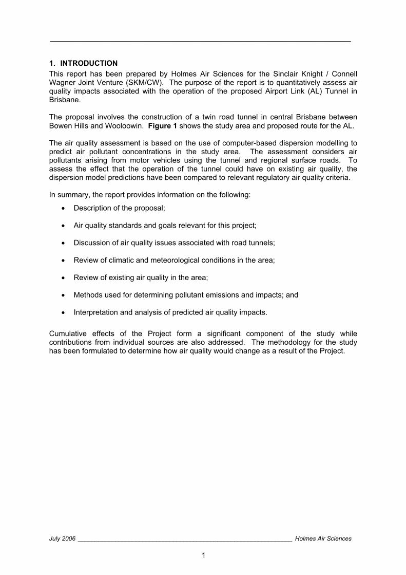
1. INTRODUCTION This report has been prepared by Holmes Air Sciences for the Sinclair Knight / Connell Wagner Joint Venture (SKM/CW). The purpose of the report is to quantitatively assess air quality impacts associated with the operation of the proposed Airport Link (AL) Tunnel in Brisbane.
The proposal involves the construction of a twin road tunnel in central Brisbane between Bowen Hills and Wooloowin. Figure 1 shows the study area and proposed route for the AL.
The air quality assessment is based on the use of computer-based dispersion modelling to predict air pollutant concentrations in the study area. The assessment considers air pollutants arising from motor vehicles using the tunnel and regional surface roads. To assess the effect that the operation of the tunnel could have on existing air quality, the dispersion model predictions have been compared to relevant regulatory air quality criteria.
In summary, the report provides information on the following:
Description of the proposal;
Air quality standards and goals relevant for this project;
Discussion of air quality issues associated with road tunnels;
Review of climatic and meteorological conditions in the area;
Review of existing air quality in the area;
Methods used for determining pollutant emissions and impacts; and
Interpretation and analysis of predicted air quality impacts.
Cumulative effects of the Project form a significant component of the study while contributions from individual sources are also addressed. The methodology for the study has been formulated to determine how air quality would change as a result of the Project.
________________________________________________________________________
July 2006 _______________________________________________________________ Holmes Air Sciences
2
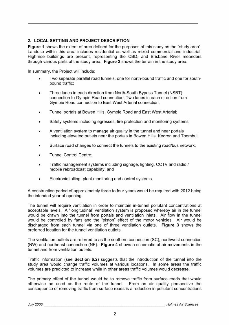
2. LOCAL SETTING AND PROJECT DESCRIPTION Figure 1 shows the extent of area defined for the purposes of this study as the “study area”. Landuse within this area includes residential as well as mixed commercial and industrial. High-rise buildings are present, representing the CBD, and Brisbane River meanders through various parts of the study area. Figure 2 shows the terrain in the study area.
In summary, the Project will include:
Two separate parallel road tunnels, one for north-bound traffic and one for south-bound traffic;
Three lanes in each direction from North-South Bypass Tunnel (NSBT) connection to Gympie Road connection. Two lanes in each direction from Gympie Road connection to East West Arterial connection;
Tunnel portals at Bowen Hills, Gympie Road and East West Arterial;
Safety systems including egresses, fire protection and monitoring systems;
A ventilation system to manage air quality in the tunnel and near portals including elevated outlets near the portals in Bowen Hills, Kedron and Toombul;
Surface road changes to connect the tunnels to the existing road/bus network;
Tunnel Control Centre;
Traffic management systems including signage, lighting, CCTV and radio / mobile rebroadcast capability; and
Electronic tolling, plant monitoring and control systems.
A construction period of approximately three to four years would be required with 2012 being the intended year of opening.
The tunnel will require ventilation in order to maintain in-tunnel pollutant concentrations at acceptable levels. A “longitudinal” ventilation system is proposed whereby air in the tunnel would be drawn into the tunnel from portals and ventilation inlets. Air flow in the tunnel would be controlled by fans and the “piston” effect of the motor vehicles. Air would be discharged from each tunnel via one of three ventilation outlets. Figure 3 shows the preferred location for the tunnel ventilation outlets.
The ventilation outlets are referred to as the southern connection (SC), northwest connection (NW) and northeast connection (NE). Figure 4 shows a schematic of air movements in the tunnel and from ventilation outlets.
Traffic information (see Section 6.2) suggests that the introduction of the tunnel into the study area would change traffic volumes at various locations. In some areas the traffic volumes are predicted to increase while in other areas traffic volumes would decrease.
The primary effect of the tunnel would be to remove traffic from surface roads that would otherwise be used as the route of the tunnel. From an air quality perspective the consequence of removing traffic from surface roads is a reduction in pollutant concentrations

________________________________________________________________________
July 2006 _______________________________________________________________ Holmes Air Sciences
3
near the surface road. It is important that the air quality impacts of the Project are based on consideration of all changes resulting from the Project. These changes may include:
Increases and decreases in surface road traffic arising from introducing a tunnel into the road network; and
Removing emissions from surface roads and venting via tunnel ventilation outlets.
________________________________________________________________________
July 2006 _______________________________________________________________ Holmes Air Sciences
4
3. AIR QUALITY STANDARDS AND GOALS In assessing any project with significant air emissions, it is necessary to compare the impacts of the project with relevant air quality goals. Air quality standards or goals are used to assess the potential for ambient air quality to give rise to adverse health or nuisance effects.
The Queensland Government Environment Protection Agency (EPA) have set air quality goals as part of their Environmental Protection (Air) Policy 1997 (EPA, 1997). The policy was developed to meet air quality objectives for Queensland’s air environment as outlined in the Environmental Protection Act 1994 (EPA, 1994).
In addition, the National Environment Protection Council of Australia (NEPC) has determined a set of air quality goals for adoption at a national level, which are part of the National Environment Protection Measures (NEPM). For the purposes of this project the EPA has proposed to adopt the NEPM air quality standards and goals either where there is no set EPA criteria or where the NEPM criteria are more stringent than the set EPA criteria.
It is important to note that the standards established as part of the NEPM are designed to be measured to give an ‘average’ representation of general air quality. That is, the NEPM monitoring protocol was not designed to apply to monitoring peak concentrations from major emission sources (NEPC, 1998).
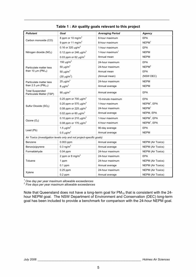
Table 1 lists the air quality goals for criteria pollutants noted by the EPA and NEPM that are relevant for this study. Also included in this table are air quality goals for air toxics developed by NEPC as part of their National Environment Protection (Air Toxics) Measure (NEPC, 2004). At this stage values for air toxics are termed “investigation levels” rather than goals which are applied on a project basis. The basis of these air quality goals and, where relevant, the safety margins that they provide are discussed in detail in Appendix A.
The primary air quality objective of most projects is to ensure that the air quality goals listed in Table 1 are not exceeded at any location where there is the possibility of human exposure for the time period relevant to the goal.
________________________________________________________________________
July 2006 _______________________________________________________________ Holmes Air Sciences
5
Table 1 : Air quality goals relevant to this project
Pollutant Goal Averaging Period Agency
Carbon monoxide (CO) 8 ppm or 10 mg/m3
9 ppm or 11 mg/m3
8-hour maximum
8-hour maximum
EPA
NEPM1
Nitrogen dioxide (NO2)
0.16 or 320 g/m3
0.12 ppm or 246 g/m3
0.03 ppm or 62 g/m3
1-hour maximum
1-hour maximum1
Annual mean
EPA
NEPM
NEPM
Particulate matter less than 10 m (PM10)
150 g/m3
50 g/m3
50 g/m3
(30 g/m3)
24-hour maximum
24-hour maximum
Annual mean
(Annual mean)
EPA
NEPM2
EPA
(NSW DEC)
Particulate matter less than 2.5 m (PM2.5)
25 g/m3
8 g/m3
24-hour maximum
Annual average
NEPM
NEPM
Total Suspended Particulate Matter (TSP) 90 g/m3 Annual average EPA
Sulfur Dioxide (SO2)
0.25 ppm or 700 g/m3
0.20 ppm or 570 g/m3
0.08 ppm or 225 g/m3
0.02 ppm or 60 g/m3
10-minute maximum
1-hour maximum
24-hour maximum
Annual average
EPA
NEPM1, EPA
NEPM1
NEPM, EPA
Ozone (O3)0.10 ppm or 210 g/m3
0.08 ppm or 170 g/m3
1-hour maximum
4-hour maximum
NEPM1, EPA
NEPM1, EPA
Lead (Pb) 1.5 g/m3
0.5 g/m3
90-day average
Annual average
EPA
NEPM
Air Toxics (investigation levels only and not project-specific goals)
Benzene 0.003 ppm Annual average NEPM (Air Toxics)
Benzo(a)pyrene 0.3 ng/m3 Annual average NEPM (Air Toxics)
Formaldehyde 0.04 ppm 24-hour maximum NEPM (Air Toxics)
Toluene
2 ppm or 8 mg/m3
1 ppm
0.1 ppm
24-hour maximum
24-hour maximum
Annual average
EPA
NEPM (Air Toxics)
NEPM (Air Toxics)
Xylene 0.25 ppm
0.2 ppm
24-hour maximum
Annual average
NEPM (Air Toxics)
NEPM (Air Toxics)
1 One day per year maximum allowable exceedances 2 Five days per year maximum allowable exceedances
Note that Queensland does not have a long-term goal for PM10 that is consistent with the 24-hour NEPM goal. The NSW Department of Environment and Conservation (DEC) long-term goal has been included to provide a benchmark for comparison with the 24-hour NEPM goal.
________________________________________________________________________
July 2006 _______________________________________________________________ Holmes Air Sciences
6
4. AIR QUALITY ISSUES ASSOCIATED WITH ROADWAY PROJECTS This section discusses air quality issues relevant to roadway projects such as a tunnel.
4.1 Changes to Air Quality One objective for roadway projects is to improve air quality or to minimise air quality impacts. It is important to review the change in air quality that is likely to occur with the Project. Assessing the change in air quality should take into account any increase or decrease in emissions in the study area due to the Project. Increases or decreases in emissions will arise as a result of a change in the traffic along a particular corridor.
On a regional scale the change in Vehicle Kilometres Travelled (VKT) in the study area will directly influence the change in air quality that would be expected in the study area.
Emissions from vehicles vary depending on a number of factors. The primary factors which influence the vehicle emissions from a roadway include:
The mode of travel (a measure of the stop/start nature of the traffic flow and the average speed);
The grade of road; and
The type of vehicles and vehicle ages.
In general, a congested road with numerous intersections will generate higher emissions than a free flowing road with no intersections. Steeper road grades generate higher emissions due to the higher engine loads, and roads with a higher percentage of heavy vehicles typically generate higher emissions.
4.2 Surface Roads and Tunnels In terms of emissions from vehicles and resultant pollutant concentrations the difference between surface roads and tunnels lies at the point of emission. Emissions from surface roads are released at ground-level where a greater proportion of the population reside. The surface road relies solely on atmospheric dispersion to reduce the pollutant concentrations between the roadway and the sensitive receptor.
In contrast, tunnel emissions are generally vented via a ventilation outlet(s) assuming that the ventilation system is operated to avoid portal emissions. The point of emission from the tunnel is therefore above ground-level (at the outlet height). This removes the plume from nearby ground-level receptors and, under poor dispersion conditions, there will be minimal impact as the plume does not spread sufficiently to reach the ground. The elevated plume also has a greater volume of atmosphere in which to disperse. An elevated point source is therefore more effective in dispersing pollution than a surface road (line source) with the same emission.
It has been seen from dispersion modelling studies (Holmes Air Sciences, 2001) that, provided the tunnel is sufficiently ventilated, significant air quality benefits can be obtained using tunnels. The most significant air quality benefits occur along surface roads which undergo the reduction in traffic as a result of the tunnel.
________________________________________________________________________
July 2006 _______________________________________________________________ Holmes Air Sciences
7
The ventilation outlets do, however, need to be sited appropriately and where possible not in valleys and not close to high rise buildings.
One of the primary impacts associated with tunnels is a negative perception of ventilation outlets. Outlets are often seen as a new pollution source whereas in most cases the surrounding areas achieve a benefit in local air quality due to the reduction of vehicles on the surface roads. In most cases tunnel ventilation outlets are not a new pollution source, rather, they redistribute existing vehicle emissions that would otherwise be released at ground-level.
4.3 Tunnel Filtration Filtration is a contentious subject for road tunnels. There are generally two types of tunnel filtration options:
In-tunnel filtration aimed at reducing pollutant concentrations for motorists using the tunnel; and
Ventilation outlet filtration aimed at reducing pollutant concentrations emitted to the outside ambient air.
Dispersion modelling studies (see Holmes Air Sciences, 2001, 2004) have indicated that, even when high levels of filtration efficiency are assumed, the differences to ambient air quality at ground-level would be small and unlikely to be detectable by conventional monitoring instrumentation. Pollutant emissions from surface roads tend to contribute more to ground-level air quality than emissions from the tunnel ventilation outlets. Ultimately, however, the most beneficial option for the treatment of emissions from motor vehicles lies at the point of emission. Controlling emissions from each individual motor vehicle ensures that benefits to air quality would be realised on regional and larger scales.
For most of this study the modelling has assumed that there would be no tunnel filtration as part of the Project. The consequence of this assumption, for the purposes of this assessment, is that estimated pollutant emissions from tunnel ventilation outlets would be higher than for a tunnel with filtration equipment fitted. The degree of difference between ventilation outlet emissions for a tunnel with and without filtration will depend on the efficiency of filtration equipment.
In addition, dispersion modelling with tunnel filtration has been conducted to provide some comparisons of the likely effects on air quality.
________________________________________________________________________
July 2006 _______________________________________________________________ Holmes Air Sciences
8
5. EXISTING ENVIRONMENT This section describes the dispersion meteorology, general climate and existing air quality of the study area. As well as information on prevailing wind patterns, historical data on temperature, humidity and rainfall are presented to give a more complete picture of the local climate.
5.1 Dispersion Meteorology The meteorology in the study area would be influenced by several factors including the local terrain and land-use. On a relatively small scale, winds would be largely affected by the local topography (see Figure 2 for a representation of the local terrain). At larger scales, winds are affected by synoptic scale winds, which are modified by sea breezes in the daytime in summer (also to a certain extent in the winter) and also by a complex pattern of regional drainage flows that develop overnight.
Given the relatively diverse terrain and landuse in the study area, differences in wind patterns at different locations in the study area would be expected. These varying wind patterns would arise as a result of the interaction of the air flow with the surrounding topography and the differential heating of the land and water. Figure 5 shows the location of meteorological monitoring sites which were used to compare localised wind patterns throughout the area.
In the air quality assessment undertaken in this report it is not necessary to document the complex mechanisms that affect air movements in the area, it is simply necessary to ensure that these air movements are incorporated into the dispersion modelling studies that are done. A limitation of common Gaussian plume dispersion models (such as AUSPLUME) is that they assume that the meteorological conditions are the same spatially over the entire modelling domain for any given hour. This may be adequate for sources in relatively uncomplicated terrain however when the terrain or landuse is more complex the meteorological conditions can be more accurately represented using wind field and puff models.
In the last decade there has been a significant improvement in the capability of dispersion models to handle dispersion in areas where complex wind flows occur. In this assessment we have made extensive use of the CALPUFF dispersion model. The CALPUFF model makes use of wind fields generated by the CALMET model. CALMET generates a three-dimensional wind field on an hourly basis by taking observations of winds at selected locations and interpolating these to produce information on wind speed and direction at a grid of regularly spaced points covering the area of interest. Modifications that are imposed on this interpolated wind field (by topography and differential heating and differential surface roughness) are then applied to the winds at each grid point to develop a final wind field.
The final wind field reflects the effect of local topography and the effects of different temperatures experienced by water bodies and land surfaces as well as different surface roughness that arise because of changes in vegetation or other variations in land use such as the presence of residential and industrial developments. Figure 6 shows the model extents, terrain and landuse information used as input to the CALMET model.
The CALMET and CALPUFF models have undergone many validation studies in Australia, New Zealand and in the United States. The CALPUFF modelling system is the US EPA’s preferred model for assessment of long range pollutant transport and for near field applications with complex meteorology. In NSW, the DEC have listed CALPUFF as an
________________________________________________________________________
July 2006 _______________________________________________________________ Holmes Air Sciences
9
“approved” air dispersion model for regulatory impact assessments (DEC, 2005). The Queensland EPA do not list “approved” air dispersion models in the EPP (Air) (1997).
Meteorological and ambient air quality monitoring data from a number of years has been reviewed to determine the most suitable year for the CALMET and CALPUFF modelling. Typically, one year of records will be sufficient to cover most variations in meteorology that will be experienced at a site, however it is important that the selected year is generally typical of the prevailing meteorology. The year 2004 was chosen for the purposes of this assessment based on the completeness of both the meteorological and ambient air quality monitoring records. The latter are required to account for background pollution levels.
A wind field has been generated by CALMET for each hour of the 2004 calendar year using meteorological data from Bureau of Meteorology (BoM) and EPA monitoring sites. Further details are discussed below. The CALMET model has essentially used the data from these sites to determine wind patterns over the entire modelling domain given information on the local landuse and terrain features.
In addition to surface meteorological records, the CALMET model requires upper air data in order to generate a year-long three-dimensional wind-field. Upper air data records collected by the BoM in 2004 at Brisbane Airport were used to provide the CALMET model with the required information on pressure changes, higher altitude winds and temperature profiles. These data included twice daily records of wind speed, wind direction, temperature, pressure and height and were processed into a form suitable for the CALMET model.
There were occasional missing soundings in the BoM upper air data for 2004 which were supplemented with upper air predictions from the CSIRO’s prognostic model (The Air Pollution Model, TAPM). TAPM is a prognostic model which has the ability to generate meteorological data for any location in Australia (from 1997 onwards) based on synoptic information determined from the six hourly Limited Area Prediction System (LAPS) (Puri etal., 1997). TAPM is further discussed in the user manual (Hurley, 2002).
Figure 7 shows a snapshot of winds simulated by the CALMET model for stable night-time conditions. The diagram shows the effect of the terrain on the flow of winds for a particular set of atmospheric conditions. The difference in wind speed and direction at various locations of the study area is evident.
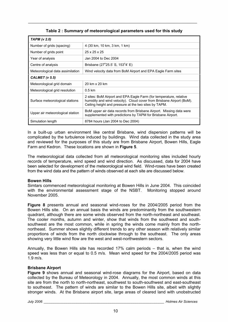
A summary of the data and parameters used as part of the meteorological component of this study are shown in Table 2.
________________________________________________________________________
July 2006 _______________________________________________________________ Holmes Air Sciences
10
Table 2 : Summary of meteorological parameters used for this study
TAPM (v 2.0)
Number of grids (spacing) 4 (30 km, 10 km, 3 km, 1 km)
Number of grids point 25 x 25 x 25
Year of analysis Jan 2004 to Dec 2004
Centre of analysis Brisbane (27o25.5’ S, 153o4’ E)
Meteorological data assimilation Wind velocity data from BoM Airport and EPA Eagle Farm sites
CALMET (v 5.5)
Meteorological grid domain 20 km x 20 km
Meteorological grid resolution 0.5 km
Surface meteorological stations 2 sites: BoM Airport and EPA Eagle Farm (for temperature, relative humidity and wind velocity). Cloud cover from Brisbane Airport (BoM). Ceiling height and pressure at the two sites by TAPM.
Upper air meteorological station BoM upper air data records from Brisbane Airport. Missing data were supplemented with predictions by TAPM for Brisbane Airport.
Simulation length 8784 hours (Jan 2004 to Dec 2004)
In a built-up urban environment like central Brisbane, wind dispersion patterns will be complicated by the turbulence induced by buildings. Wind data collected in the study area and reviewed for the purposes of this study are from Brisbane Airport, Bowen Hills, Eagle Farm and Kedron. These locations are shown in Figure 5.
The meteorological data collected from all meteorological monitoring sites included hourly records of temperature, wind speed and wind direction. As discussed, data for 2004 have been selected for development of the meteorological wind field. Wind-roses have been created from the wind data and the pattern of winds observed at each site are discussed below.
Bowen Hills Simtars commenced meteorological monitoring at Bowen Hills in June 2004. This coincided with the environmental assessment stage of the NSBT. Monitoring stopped around November 2005.
Figure 8 presents annual and seasonal wind-roses for the 2004/2005 period from the Bowen Hills site. On an annual basis the winds are predominantly from the southwestern quadrant, although there are some winds observed from the north-northeast and southeast. The cooler months, autumn and winter, show that winds from the southwest and south-southwest are the most common, while in spring the winds come mainly from the north-northeast. Summer shows slightly different trends to any other season with relatively similar proportions of winds from the north clockwise through to the southeast. The only areas showing very little wind flow are the west and west-northwestern sectors.
Annually, the Bowen Hills site has recorded 17% calm periods – that is, when the wind speed was less than or equal to 0.5 m/s. Mean wind speed for the 2004/2005 period was 1.9 m/s.
Brisbane Airport Figure 9 shows annual and seasonal wind-rose diagrams for the Airport, based on data collected by the Bureau of Meteorology in 2004. Annually, the most common winds at this site are from the north to north-northeast, southwest to south-southwest and east-southeast to southeast. The pattern of winds are similar to the Bowen Hills site, albeit with slightly stronger winds. At the Brisbane airport site, large areas of cleared land with unobstructed
________________________________________________________________________
July 2006 _______________________________________________________________ Holmes Air Sciences
11
wind flow, will result in higher than average local wind speeds compared to the surrounding residential and industrial areas.
In summer, winds at the airport are predominantly from the north which is a typical sea breeze condition. The sea breeze usually commences in the late morning and is well established in the afternoon. Spring exhibits a similar pattern to summer.
In contrast to summer and spring, the most common winds in autumn and winter are from the southwest and south-southwest.
The average wind speed in 2004 at the airport was 4.4 m/s with a maximum hourly average wind speed of 13.3 m/s. The frequency of calm conditions was 2.2%.
Eagle Farm Figure 10 presents annual and seasonal wind-roses for 2004 data from Eagle Farm. The distribution of winds for Eagle Farm on an annual and seasonal basis is similar to that at both Bowen Hills and Brisbane Airport. This would be expected given the relatively close proximity of the Eagle Farm site to the other sites – less than approximately five kilometres.
Eagle Farm typically has lower wind speeds than the Airport with a maximum hourly average wind speed of 7.3 m/s and an annual average of 2.0 m/s. The percentage of calms is 8.4%. The lower speed winds at the Bowen Hills and Eagle Farm sites are consistent with their location within residential and industrial areas, where buildings and terrain provide some shielding from the prevailing winds, compared with the more exposed BoM Airport site.
The similarities in the wind data for both Eagle Farm and Bowen Hills may be expected given that there are not many significant terrain features between the two sites.
KedronCollection of meteorological data in the vicinity of the proposed northwest connection of the AL commenced in January 2006. These data will provide additional information on wind patterns in the central part of the study area and will be analysed as they become available.
For the purposes of this study the Airport and Eagle Farm data have been considered to be the most suitable datasets for CALMET to establish wind patterns over the entire study area. This is based on the completeness of the monitoring records for the CALMET simulation year. Also, the proximity of these sites to the area of interest ensures that they would contain data that are representative of the dispersion conditions in the study area. Furthermore, the data from Eagle Farm and Bowen Hills show a similar distribution of winds.
________________________________________________________________________
July 2006 _______________________________________________________________ Holmes Air Sciences
12
5.2 Atmospheric Stability Dispersion models typically require information on atmospheric stability class1 and mixing height2. Plume dispersion models usually assume that the atmospheric stability is uniform over the entire study domain and these estimates are commonly calculated from measurements of sigma-theta, cloud cover information or solar radiation and temperature. Hourly estimates of mixing height can be determined by a combination of empirical methods and/or soundings.
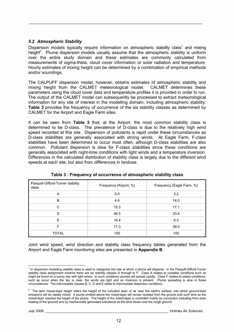
The CALPUFF dispersion model, however, obtains estimates of atmospheric stability and mixing height from the CALMET meteorological model. CALMET determines these parameters using the cloud cover data and temperature profiles it is provided in order to run. The output of the CALMET model can subsequently be processed to extract meteorological information for any site of interest in the modelling domain, including atmospheric stability. Table 3 provides the frequency of occurrence of the six stability classes as determined by CALMET for the Airport and Eagle Farm sites.
It can be seen from Table 3 that, at the Airport, the most common stability class is determined to be D-class. The prevalence of D-class is due to the relatively high wind speed recorded at this site. Dispersion of pollutants is rapid under these circumstances as D-class stabilities are generally associated with strong winds. At Eagle Farm, F-class stabilities have been determined to occur most often, although D-class stabilities are also common. Pollutant dispersion is slow for F-class stabilities since these conditions are generally associated with night-time conditions with light winds and a temperature inversion. Differences in the calculated distribution of stability class is largely due to the different wind speeds at each site, but also from differences in landuse.
Table 3 : Frequency of occurrence of atmospheric stability class
Pasquill-Gifford-Turner stability class Frequency (Airport, %) Frequency (Eagle Farm, %)
A 0.0 3.2
B 4.4 14.0
C 15.3 17.1
D 46.5 20.4
E 16.4 6.3
F 17.3 39.0
TOTAL 100 100
Joint wind speed, wind direction and stability class frequency tables generated from the Airport and Eagle Farm monitoring sites are presented in Appendix B.
1 In dispersion modelling stability class is used to categorise the rate at which a plume will disperse. In the Pasquill-Gifford-Turnerstability class assignment scheme there are six stability classes A through to F. Class A relates to unstable conditions such asmight be found on a sunny day with light winds. In such conditions plumes will spread rapidly. Class F relates to stable conditions,such as occur when the sky is clear, the winds are light and an inversion is present. Plume spreading is slow in these circumstances. The intermediate classes B, C, D and E relate to intermediate dispersion conditions.
2 The term mixed-layer height refers the height of the turbulent layer of air near the earth's surface, into which ground-levelemissions will be rapidly mixed. A plume emitted above the mixed-layer will remain isolated from the ground until such time as the mixed-layer reaches the height of the plume. The height of the mixed-layer is controlled mainly by convection (resulting from solar heating of the ground) and by mechanically generated turbulence as the wind blows over the rough ground.

________________________________________________________________________
July 2006 _______________________________________________________________ Holmes Air Sciences
13
5.3 Local Climatic Conditions The Bureau of Meteorology collects climatic information from Brisbane Aerodrome, to the east of the study area. A range of meteorological data collected from this station are presented in Table 4 (Bureau of Meteorology, 2006). Temperature and humidity data consist of monthly averages of 9 am and 3 pm readings. Also presented are monthly averages of maximum and minimum temperatures. Rainfall data consist of mean and median monthly rainfall and the average number of raindays per month.
Table 4 : Climate information for the study area
Brisbane Aerodrome Jan Feb Mar Apr May Jun Jul Aug Sep Oct Nov Dec Annual
Mean daily maximum temperature ( C) 29.1 28.9 28.1 26.3 23.5 21.2 20.6 21.7 23.8 25.6 27.3 28.6 25.4
Mean daily minimum temperature ( C) 20.9 20.9 19.5 16.9 13.8 10.9 9.5 10 12.5 15.6 18 19.8 15.7
Mean 9am air temp ( C) 25.7 25.3 24.1 21.5 18 15.1 14.1 15.5 18.9 21.9 23.9 25.3 20.8
Mean 9am wet bulb temp ( C) 21.4 21.5 20.5 18.1 15 12.3 11.1 12 14.6 17.1 18.9 20.5 16.9
Mean 9am relative humidity (%) 67 70 71 70 71 70 68 63 60 60 61 63 66
Mean 3pm air temp ( C) 27.6 27.5 26.7 25 22.4 20.2 19.6 20.6 22.4 23.9 25.6 26.9 24
Mean 3pm wet bulb temp ( C) 22 22.1 21.2 19.2 16.7 14.5 13.6 14.1 15.9 18 19.7 21.3 18.2
Mean 3pm relative humidity (%) 60 61 60 57 55 51 48 45 48 54 57 59 55
Mean monthly rainfall (mm) 157.7 171.7 138.5 90.4 98.8 71.2 62.6 42.7 34.9 94.4 96.5 126.2 1185
Mean no. of raindays 13 14.2 14.1 11 10.5 7.5 7.2 6.6 6.9 10 10 11.5 122.4
Mean daily evaporation (mm) 7.3 6.5 5.8 4.5 3.2 3 3.2 4.1 5.5 6.3 7.2 7.5 5.3
Mean no. of clear days 4.6 4 8.1 9.8 10.8 13 15 16.7 15.6 10.1 8 6.7 122.4
Mean no. of cloudy days 12.4 12.6 11.6 8.6 9.7 7.5 7 5.5 5.1 8.5 9.7 10.5 108.6
Mean daily hours of sunshine 8.5 7.5 7.7 7.4 6.4 7.2 7.4 8.4 8.9 8.5 8.6 8.8 8
Climate averages for Station: 040223 BRISBANE AERO, Commenced: 1929; Last record: 2000; Latitude (deg S): -27.4178; Longitude (deg E): 153.1142; State: QLD. Source: Bureau of Meteorology, 2006
In summer the average maximum temperature ranges from 28.6°C to 29.1°C and the minimum temperature ranges from 19.8°C to 20.9°C. In winter the average maximum temperature ranges from 20.6°C to 21.7°C and the minimum temperature ranges from 9.5°C to 10.9°C.
The annual average humidity reading collected at 9 am from the Brisbane Aerodrome site is 66 percent, and at 3 pm the annual average is 55 percent. The months with the highest humidity on average are March and May with a 9 am averages of 71 percent, and the lowest is August with a 3 pm average of 45 percent.
________________________________________________________________________
July 2006 _______________________________________________________________ Holmes Air Sciences
14
Rainfall data collected at Brisbane Aerodrome shows that the wettest month is February, during the wetter summer season, with an average rainfall of 171.7 mm over 14.2 days. The lowest rainfall on average is in September, at the end of the winter dry season, with a mean monthly rainfall of 34.9 mm over 6.9 raindays. The average annual rainfall is 1185 mm over an average of 122 raindays.
The data from Table 4 show that the climate in Brisbane is characterised by wet summers and low rainfall in winter. This is typical of the subtropical climate of southeast Queensland.
From November to April the weather in Brisbane is warm, humid and windy with high rainfall and storms. These conditions encourage dispersion of pollutants in the air and the rain absorbs gases and particulate matter, removing them from the air. In the cooler months from May to October, there is less rain and the wind is not as strong, so there is less dispersion of pollutants.
5.4 Existing Air Quality This section discusses the concept of background air pollution as it applies to this study and presents a review of air quality monitoring data that can be used to estimate background pollution levels.
5.4.1 Accounting for Background One of the most difficult aspects in air quality assessments is accounting for the existing levels of pollutants from sources that are not included in the dispersion model. At any location within the airshed the concentration of the pollutant is determined by the contributions from all sources that have at some stage or another been upwind of the source. In the case of PM10 for example, the background concentration may contain emissions from the combustion of wood from domestic heating, from bushfires, from industry, other roads, wind blown dust from nearby and remote areas, fragments of pollens, moulds, sea-salts and so on.
In an area such as the Brisbane airshed the background level of pollutants could also include recirculated pollutants which have moved through complicated pathways in sea breeze/land breeze cycles. In general, the further away a particular source is from the area of interest, the smaller will be its contribution to air pollution at the area of interest. However the larger the area considered the greater would be the number of sources contributing to the background.
At any particular location the concentration of a pollutant will vary with time as the dispersion conditions change and as the contributing emission sources change. Including the effects of existing background pollution is difficult in all air quality studies and necessarily involves some approximations. If all emission sources can be included in the modelling study then the problem is very much simplified. When this can be done (that is, all sources are included) the background can be assumed to be zero and the total concentration is accurately represented by the model predictions. In an urban area, with common pollutants such as those from roads it is not possible to include all sources in the model. However, the greater the proportion of relevant emissions that can be included in the model then the smaller is the allowance that needs to be made for background levels and the more accurate the final estimates (predictions plus background) are likely to be.
For the Brisbane AL Project it is necessary to consider emissions from local surface roads, from the tunnel ventilation, from more distant roads and from all other non-transport related emissions of each pollutant. The emissions that will change as a result of the Project are
________________________________________________________________________
July 2006 _______________________________________________________________ Holmes Air Sciences
15
emissions from the local surface roads which will experience changed traffic flows as the traffic is redistributed between the tunnel and the local surface roads and as new traffic is brought into the area by the increased capacity of the network provided by the tunnel.
5.4.2 Air Quality Monitoring Data from three air quality monitoring sites have been assessed for the purposes of this study – Eagle Farm, Bowen Hills and Kedron. Situated at various locations around the proposed tunnel route, these sites are considered to be representative of the existing air quality environment.
The monitoring sites are summarised as follows:
Eagle Farm, operated by the EPA but now decommissioned, included measurements of NOx, O3, SO2 and PM10.
Bowen Hills, operated by Simtars but now decommissioned, included measurements of CO, NOx, PM10 and PM2.5.
Kedron, currently monitoring and operated by Simtars. Measurements include CO, NOx, PM10 and PM2.5.
The Eagle Farm site was located in a light industrial area at the DPI Quarantine Centre and was decommissioned in mid 2005. A site at Pinkenba commenced operation in 2001 and has essentially replaced the Eagle Farm site.
The Bowen Hills site was located to the north of Campbell Street in the vicinity of the proposed southern connection. This station was decommissioned in November 2005 and moved to its current position at Kedron. Monitoring commenced at Kedron in mid January 2006. These data will be reviewed as the information becomes available.
In addition, the Queensland EPA operate monitoring stations at Brisbane CBD, Rocklea, South Brisbane and Woolloongabba. Data from these sites were reviewed as part of the NSBT air quality assessment (Holmes Air Sciences, 2004) but have not undergone a major investigation for this study.
Table 5 summarises each of the air pollutants and compares these data with the relevant air quality goal.
________________________________________________________________________
July 2006 _______________________________________________________________ Holmes Air Sciences
16
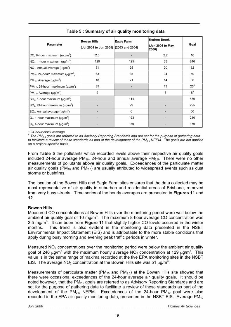
Table 5 : Summary of air quality monitoring data
ParameterBowen Hills
(Jul 2004 to Jun 2005)
Eagle Farm
(2003 and 2004)
Kedron Brook
(Jan 2006 to May 2006)
Goal
CO, 8-hour maximum (mg/m3) 2.5 - 2.2 10
NO2, 1-hour maximum ( g/m3) 129 125 83 246
NO2, Annual average ( g/m3) 51 25 20 62
PM10, 24-hour* maximum ( g/m3) 63 85 34 50
PM10, Average ( g/m3) 18 21 14 30
PM2.5, 24-hour* maximum ( g/m3) 35 - 13 25#
PM2.5, Average ( g/m3) 9 - 6 8#
SO2, 1-hour maximum ( g/m3) - 114 - 570
SO2, 24-hour maximum ( g/m3) - 29 - 225
SO2, Annual average ( g/m3) - 6 - 60
O3, 1-hour maximum ( g/m3) - 193 - 210
O3, 4-hour maximum ( g/m3) - 150 - 170
* 24-hour clock average # The PM2.5 goals are referred to as Advisory Reporting Standards and are set for the purpose of gathering data to facilitate a review of these standards as part of the development of the PM2.5 NEPM. The goals are not applied on a project-specific basis.
From Table 5 the pollutants which recorded levels above their respective air quality goals included 24-hour average PM10, 24-hour and annual average PM2.5. There were no other measurements of pollutants above air quality goals. Exceedances of the particulate matter air quality goals (PM10 and PM2.5) are usually attributed to widespread events such as dust storms or bushfires.
The location of the Bowen Hills and Eagle Farm sites ensures that the data collected may be most representative of air quality in suburban and residential areas of Brisbane, removed from very busy streets. Time series of the hourly averages are presented in Figures 11 and 12.
Bowen Hills Measured CO concentrations at Bowen Hills over the monitoring period were well below the ambient air quality goal of 10 mg/m3. The maximum 8-hour average CO concentration was 2.5 mg/m3. It can been from Figure 11 that slightly higher CO levels occurred in the winter months. This trend is also evident in the monitoring data presented in the NSBT Environmental Impact Statement (EIS) and is attributable to the more stable conditions that apply during busy morning and evening peak traffic periods in winter.
Measured NO2 concentrations over the monitoring period were below the ambient air quality goal of 246 g/m3 with the maximum hourly average NO2 concentration at 129 g/m3. This value is in the same range of maxima recorded at the five EPA monitoring sites in the NSBT EIS. The average NO2 concentration at the Bowen Hills site was 51 g/m3.
Measurements of particulate matter (PM10 and PM2.5) at the Bowen Hills site showed that there were occasional exceedances of the 24-hour average air quality goals. It should be noted however, that the PM2.5 goals are referred to as Advisory Reporting Standards and are set for the purpose of gathering data to facilitate a review of these standards as part of the development of the PM2.5 NEPM. Exceedances of the 24-hour PM10 goal were also recorded in the EPA air quality monitoring data, presented in the NSBT EIS. Average PM10
________________________________________________________________________
July 2006 _______________________________________________________________ Holmes Air Sciences
17
concentrations at Bowen Hills (18 g/m3) were similar to those reported in the EIS (between 17 and 28 g/m3) and below the 30 g/m3 air quality goal.
Eagle Farm Figure 12 shows the time series of monitoring data from Eagle Farm. Measured SO2 levels were well below the 570 g/m3 goal. There are some infrequent spikes in the hourly data which reach about a quarter of the goal. There are no significant seasonal trends evident in these data.
Concentrations of NO2 have been below the 246 g/m3 goal – the maximum hourly average for 2003 and 2004 was 125 g/m3.
The one hourly average ozone goal was almost reached late in 2004 with a measurement of 193 g/m3 compared with the goal of 210 g/m3.
Measurements of PM10 at Eagle Farm have indicated four exceedances of the 50 g/m3 goal for 24-hour averages over the 2003 and 2004 period. Historical EPA data, as presented in the NSBT EIS, have shown that many EPA sites in the Brisbane region record occasional exceedances of the 24-hour PM10 goal each year.
The measured concentrations of each pollutant are determined by all sources that at some stage have been upwind of the monitoring station. CO and NOx nitrogen would have predominately originated from motor vehicle emissions in this area. In the case of particulate matter (PM10), a number of different types of sources would have contributed to the PM10 measurements. These sources may have included emissions from bushfires, industry, motor vehicles, wind blown dust from nearby and remote areas, fragments of pollens, moulds, sea-salts and so on.
Some analysis of the percentage of NOx which has been converted to NO2 is particularly useful for roadway associated projects as estimates of NO2 concentrations are commonly derived from NOx predictions.
Nitrogen oxides are produced in most combustion processes and are formed during the oxidation of nitrogen in the fuel and nitrogen in the air. During high-temperature processes a variety of nitrogen oxides are formed including nitric oxide (NO) and NO2. Generally, at the point of emission NO will comprise the greatest proportion of the emission with 95% by volume of the NOx. The remaining 5% will be mostly NO2. The effects of NO on human health are such that it is not regarded as an air pollutant at the concentrations at which it is normally found in the environment. The presence of NOx emissions can be of concern in urban environments where the control of photochemical smog is important.
Ultimately, however, all nitric oxides emitted into the atmosphere are oxidised to NO2 and then further to other higher oxides of nitrogen. The rate at which this oxidisation takes place depends on prevailing atmospheric conditions including temperature, humidity and the presence of other substances in the atmosphere such as ozone. It can vary from a few minutes to many hours. The rate of conversion is quite important because from the point of emission to the point of maximum ground-level concentration there will be an interval of time during which some oxidation will take place. If the dispersion is sufficient to have diluted the plume to the point where the concentration is very low it is unimportant that the oxidation has taken place. However, if the oxidation is rapid and the dispersion slow then high concentrations of NO2 can occur.
Analysis of the NOx monitoring data reveals that the percentage of NO2 in the air is inversely proportional to the total NOx concentration. Figure 13 shows this relationship for Eagle
________________________________________________________________________
July 2006 _______________________________________________________________ Holmes Air Sciences
18
Farm and Bowen Hills. The ratios of NO2 to NOx in the data had average values of 65% and 55% from the Eagle Farm and Bowen Hills sites respectively. These ratios (65% and 55%) do not necessarily reflect the proportion of NO2 which would be present very close to the emission source. Many studies (see for example Pacific Power, 1998 and PPK, 1999)have reported that when NOx levels are high, the proportion of NO2 is low. Monitoring data collected by the RTA in Sydney (Holmes Air Sciences, 1997) are also consistent with this trend and indicate that close to roadways (within 60 metres), nitrogen dioxide would make up from 5 to 20% by weight of the total oxides of nitrogen.
For comparison, the EPA’s South Brisbane air quality monitoring site is adjacent to the South-East Freeway and was located to collect information at the boundary of major traffic corridors. In 2001/2002 the average NO2 to NOx fraction from this site was 39% (HolmesAir Sciences, 2004).
Generally, for plumes impacting close to the source, the time interval for oxidation is not sufficient to have converted a large proportion of the plume to the more harmful NO2. For the assessment in this study it has been assumed that the ratio of NO2 to NOx would be 10% by weight within the tunnel. This is consistent with the maximum NO2:NOx ratios reported in a detailed joint study within the Sydney Harbour Tunnel (NSW EPA, CSIRO, RTA, 1996).This ratio has been assumed to increase to 20% by the time that the plume has reached the point where the maximum ground-level or above ground-level concentrations are predicted. This is a realistic but conservative assumption, as will be seen later in Section 8.2, given that the time of day when maximum levels occur is when conversion rates are likely to be low. At locations close to the ventilation tunnel outlets (within 50 metres) it is likely that the conversion rate would result in a ratio closer to 15%. For annual average predictions of NO2, 39% of the NOx concentration is taken to be NO2.
Graphs of PM10 (Figures 11 and 12) highlight the occasions when 24-hour concentrations were above their respective air quality goals. Bowen Hills is the only site to concurrently measure PM10 and PM2.5. It can be seen from the graphs that exceedances of both the PM10and PM2.5 goals were recorded on the same days, signifying the relationship between the two particulate matter classifications. The high PM10 level around August 2004 (54 g/m3 on 10 Aug to be precise) suggest that the exceedance is from a combustion source where the percentage of PM2.5 would be relatively high. On 3 Feb 2005 the 24-hour average PM10 was 63 g/m3 and the fraction of PM2.5 was much lower than the previous event. A major dust storm in Brisbane was reported by the Bureau of Meteorology on 3 Feb 2005 (www.bom.gov.au ).
Figure 14 shows the relationship between measured PM10 and PM2.5 concentrations at the Bowen Hills site for the 2004 to 2005 period. The average ratio of PM2.5 to PM10 for the monitoring period was calculated to be 50%. Typically, the highest PM2.5 to PM10 ratios are measured in areas where combustion sources (for example, traffic) are dominant.
________________________________________________________________________
July 2006 _______________________________________________________________ Holmes Air Sciences
19
6. ESTIMATION OF POLLUTANT EMISSIONS FROM ROADS This section provides information relating to the estimation of pollutant emissions from a road section with known traffic volume. Sources of emission factors are discussed as well as the traffic information used in the study. A summary of the calculated pollutant emissions for the tunnel and various surface roads is provided in this section.
6.1 Emission Data The most significant emissions produced from motor vehicles are CO, NOx, hydrocarbons and PM10. Estimated emissions of these pollutants are required as input to computer-based dispersion models in order to predict pollutant concentrations in the area of interest and to compare these concentrations with associated air quality goals.
As discussed in Section 4, the primary factors which influence emissions from vehicles include the mode of travel, the grade of the road and the mix or type of vehicles on the road. It is important to estimate pollutant emissions using as much information as is known about these factors.
The general approach to derive total pollutant emissions from a road section is simply to multiply the total number of vehicles on the road section by the pollutant emission per vehicle (the emission factor). Pollutant emission factors are typically provided in units of grams per kilometre or sometimes as grams per hour. There are a number of sources of these emission factors.
Sources of emission factors which have been referenced for the purposes of this project include:
World Road Association, referred to as PIARC (formerly the Permanent International Association of Road Congress); and
The South-east Queensland Region Air Emissions Inventory.
6.1.1 PIARC PIARC is a European-based organisation focused on road transport related issues. Technical committees coordinated by PIARC regularly circulate documents on many aspects of roads and road transport, including road tunnels.
In 1995, PIARC published a document (PIARC, 1995) as the basis of design for longitudinal tunnel ventilation systems. The document, entitled “Vehicle emissions, air demand, environment, longitudinal ventilation”, also provided comprehensive vehicle emissions factors for different road gradients, vehicle speeds and for vehicles conforming to different European emission standards. Given the detailed emission breakdowns, the PIARC data are very useful for sensitivity testing, such as analysing the effect of changes to road grade, and are particularly relevant for emission estimation from road tunnels.
The 1995 PIARC document described the emission situation up to the year 1995. In 2004, PIARC updated the methodology and emissions information (PIARC, 2004) based on activities between 2001 and 2003. The design data are subject to ongoing review due to a steady tightening of emission standard for vehicles.
________________________________________________________________________
July 2006 _______________________________________________________________ Holmes Air Sciences
20
Since the PIARC emissions data are primarily based on European studies, the emission tables have been modified to take account of the age, vehicle mix, vehicle speed, gradient of road and emissions control technology of the Australian vehicle fleet. The modified tables include emissions of CO, NOx and PM10 by age and type of vehicle. The age of vehicles have been categorised into five periods, corresponding to the introduction of emission standards, and three vehicle type categories.
The vehicle types have been defined as follows:
Passenger cars using petrol;
Passenger cars using diesel; and
Heavy goods vehicles using diesel.
The general approach for using the PIARC data was to combine total traffic volume with percentages of vehicles in each age bracket and type category. Using these inputs, as well as road grade and speed information, total emissions for selected sections of road have been generated.
Further details on how the PIARC emission data were related to the Australian vehicle fleet are provided in Appendix C.
6.1.2 South-east Queensland Region Air Emissions Inventory A partnership between the Brisbane City Council (BCC) and the EPA produced a local Queensland vehicle emission database as part of the South-east Queensland region Air Emissions Inventory (EPA & BCC, 2004). Included in this database are estimates of current vehicle emission rates as well as projections to future years.
It is understood that the development of the vehicle emissions database has taken into consideration future vehicle design rules and likely fuel standards. Emission rates are provided for the south-east Queensland region for 2000 for different vehicle types. In addition, fleet-average exhaust emission factors are provided for 2005 and 2011.
For the purposes of this study the vehicle emission data from the South-east Queensland region Air Emissions Inventory have been used for comparative purposes with the PIARC data. The PIARC information has been the primary emission data source. Appendix Cprovides some comparisons of vehicle emissions generated for the south-east Queensland region using both the PIARC methodology and the Air Emissions Inventory data. The comparison indicated that the two data sources generally resulted in similar emission rates for future years, the PIARC methodology adopted for this study was found to be slightly more conservative.
6.2 Traffic Data SKM/CW generated traffic information for the Project. The traffic data made available and used for the purposes of the air quality study included the following:
AADT for years 2004 (existing), 2012, 2016 and 2026;
Scenarios “without AL”, “with AL” and “with AL and Northern Busway”;
Modelled existing (2004) AADT for selected surface roads;
________________________________________________________________________
July 2006 _______________________________________________________________ Holmes Air Sciences
21
Modelled 2012, 2016 and 2026 AADT for selected surface roads; and
Indicative flow profiles for light and heavy vehicles by hour of day for each section of tunnel and for surface roads.
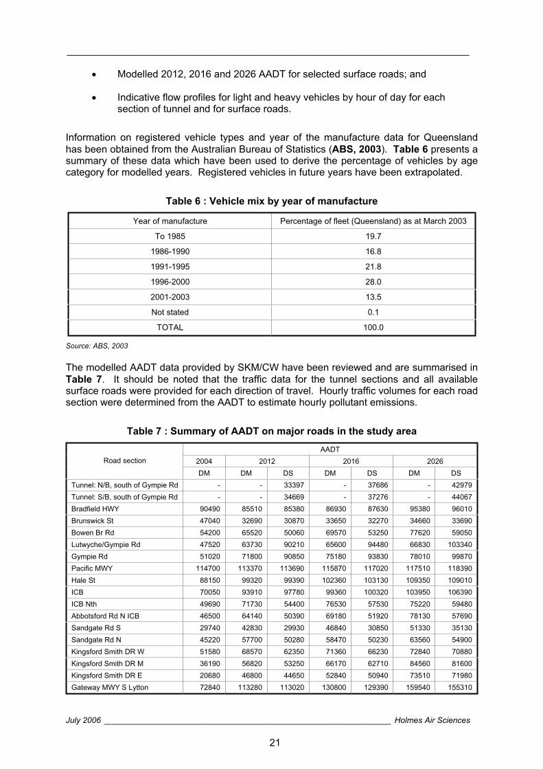
Information on registered vehicle types and year of the manufacture data for Queensland has been obtained from the Australian Bureau of Statistics (ABS, 2003). Table 6 presents a summary of these data which have been used to derive the percentage of vehicles by age category for modelled years. Registered vehicles in future years have been extrapolated.
Table 6 : Vehicle mix by year of manufacture
Year of manufacture Percentage of fleet (Queensland) as at March 2003
To 1985 19.7
1986-1990 16.8
1991-1995 21.8
1996-2000 28.0
2001-2003 13.5
Not stated 0.1
TOTAL 100.0
Source: ABS, 2003
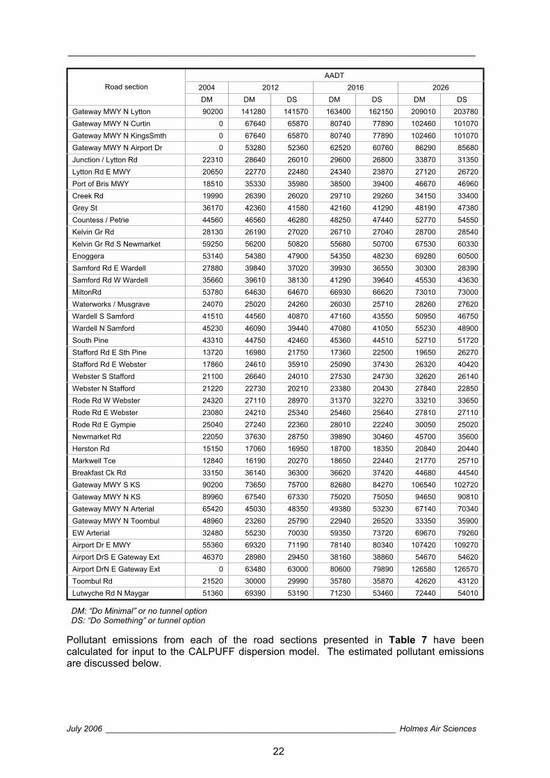
The modelled AADT data provided by SKM/CW have been reviewed and are summarised in Table 7. It should be noted that the traffic data for the tunnel sections and all available surface roads were provided for each direction of travel. Hourly traffic volumes for each road section were determined from the AADT to estimate hourly pollutant emissions.
Table 7 : Summary of AADT on major roads in the study area
AADT2004 2012 2016 2026 Road section
DM DM DS DM DS DM DS Tunnel: N/B, south of Gympie Rd - - 33397 - 37686 - 42979 Tunnel: S/B, south of Gympie Rd - - 34669 - 37276 - 44067 Bradfield HWY 90490 85510 85380 86930 87630 95380 96010 Brunswick St 47040 32690 30870 33650 32270 34660 33690 Bowen Br Rd 54200 65520 50060 69570 53250 77620 59050 Lutwyche/Gympie Rd 47520 63730 90210 65600 94480 66830 103340 Gympie Rd 51020 71800 90850 75180 93830 78010 99870 Pacific MWY 114700 113370 113690 115870 117020 117510 118390 Hale St 88150 99320 99390 102360 103130 109350 109010 ICB 70050 93910 97780 99360 100320 103950 106390 ICB Nth 49690 71730 54400 76530 57530 75220 59480 Abbotsford Rd N ICB 46500 64140 50390 69180 51920 78130 57690 Sandgate Rd S 29740 42830 29930 46840 30850 51330 35130 Sandgate Rd N 45220 57700 50280 58470 50230 63560 54900 Kingsford Smith DR W 51580 68570 62350 71360 66230 72840 70880 Kingsford Smith DR M 36190 56820 53250 66170 62710 84560 81600 Kingsford Smith DR E 20680 46800 44650 52840 50940 73510 71980 Gateway MWY S Lytton 72840 113280 113020 130800 129390 159540 155310
________________________________________________________________________
July 2006 _______________________________________________________________ Holmes Air Sciences
22
AADT2004 2012 2016 2026 Road section
DM DM DS DM DS DM DS Gateway MWY N Lytton 90200 141280 141570 163400 162150 209010 203780 Gateway MWY N Curtin 0 67640 65870 80740 77890 102460 101070 Gateway MWY N KingsSmth 0 67640 65870 80740 77890 102460 101070 Gateway MWY N Airport Dr 0 53280 52360 62520 60760 86290 85680 Junction / Lytton Rd 22310 28640 26010 29600 26800 33870 31350 Lytton Rd E MWY 20650 22770 22480 24340 23870 27120 26720 Port of Bris MWY 18510 35330 35980 38500 39400 46670 46960 Creek Rd 19990 26390 26020 29710 29260 34150 33400 Grey St 36170 42360 41580 42160 41290 48190 47380 Countess / Petrie 44560 46560 46280 48250 47440 52770 54550 Kelvin Gr Rd 28130 26190 27020 26710 27040 28700 28540 Kelvin Gr Rd S Newmarket 59250 56200 50820 55680 50700 67530 60330 Enoggera 53140 54380 47900 54350 48230 69280 60500 Samford Rd E Wardell 27880 39840 37020 39930 36550 30300 28390 Samford Rd W Wardell 35660 39610 38130 41290 39640 45530 43630 MiltonRd 53780 64630 64670 66930 66620 73010 73000 Waterworks / Musgrave 24070 25020 24260 26030 25710 28260 27620 Wardell S Samford 41510 44560 40870 47160 43550 50950 46750 Wardell N Samford 45230 46090 39440 47080 41050 55230 48900 South Pine 43310 44750 42460 45360 44510 52710 51720 Stafford Rd E Sth Pine 13720 16980 21750 17360 22500 19650 26270 Stafford Rd E Webster 17860 24610 35910 25090 37430 26320 40420 Webster S Stafford 21100 26640 24010 27530 24730 32620 26140 Webster N Stafford 21220 22730 20210 23380 20430 27840 22850 Rode Rd W Webster 24320 27110 28970 31370 32270 33210 33650 Rode Rd E Webster 23080 24210 25340 25460 25640 27810 27110 Rode Rd E Gympie 25040 27240 22360 28010 22240 30050 25020 Newmarket Rd 22050 37630 28750 39890 30460 45700 35600 Herston Rd 15150 17060 16950 18700 18350 20840 20440 Markwell Tce 12840 16190 20270 18650 22440 21770 25710 Breakfast Ck Rd 33150 36140 36300 36620 37420 44680 44540 Gateway MWY S KS 90200 73650 75700 82680 84270 106540 102720 Gateway MWY N KS 89960 67540 67330 75020 75050 94650 90810 Gateway MWY N Arterial 65420 45030 48350 49380 53230 67140 70340 Gateway MWY N Toombul 48960 23260 25790 22940 26520 33350 35900 EW Arterial 32480 55230 70030 59350 73720 69670 79260 Airport Dr E MWY 55360 69320 71190 78140 80340 107420 109270 Airport DrS E Gateway Ext 46370 28980 29450 38160 38860 54670 54620 Airport DrN E Gateway Ext 0 63480 63000 80600 79890 126580 126570 Toombul Rd 21520 30000 29990 35780 35870 42620 43120 Lutwyche Rd N Maygar 51360 69390 53190 71230 53460 72440 54010
DM: “Do Minimal” or no tunnel option DS: “Do Something” or tunnel option
Pollutant emissions from each of the road sections presented in Table 7 have been calculated for input to the CALPUFF dispersion model. The estimated pollutant emissions are discussed below.
________________________________________________________________________
July 2006 _______________________________________________________________ Holmes Air Sciences
23
6.3 Emission Estimates Pollutant emissions have been estimated for each tunnel ventilation outlet and for all surface roads discussed in Section 6.2. No potential future improvements in vehicle technology or fuel standards have been included in the PIARC emission estimates. This will result in some overestimation of emission rates for future years and tend to exaggerate the absolute difference between the “without AL” and “with AL” case. Assumed reductions in the proportion of older vehicles in the fleet has, however, simulated some improvement to vehicle emissions in future years.
In order to determine emissions from a ventilation outlet, the source of air which leads into the outlet has been considered (refer to Figure 4 for a schematic of air movements in the tunnel). The air in the outlet comes from sections of tunnel which have a traffic volume, traffic mix, traffic speed and road grade. These data are included in the process to generate pollutant emissions for each hour of the day for each outlet. Road grade information for each section of tunnel has been provided by SKM/CW.
Traffic speed within the tunnel has been set to 80 km/h outside peak-hour periods. During peak-hour periods a speed of 20 km/h has been used. For this study peak-hour periods in the tunnel have been defined as hours ending 7, 8, 9, 16, 17, 18 and 19 for both directions in the tunnel.
The peak-hour or “congested” periods are consistent with the hours selected for the Cross City Tunnel EIS in Sydney (RTA, 2000). A speed of 80 km/h has been assumed for vehicles on the motorways while 50 km/h has been assumed for all other surface roads.
Figure 15 shows the estimated traffic and pollutant emissions (CO, NOx and PM10) for each hour of the day for the AL in 2012. The profile of emission rates closely follows the traffic profile however the emission rates are also influenced by other factors such as the grade in the tunnel, speed of traffic and the proportion of heavy vehicles in the traffic mix.
Table 8 to Table 10 provide estimated pollutant emissions from the three ventilation outlets. Similar information is also required by the dispersion model for all the modelled surface roads. Emissions data for all surface roads are not included in the body of this report for ease of reading but the calculations are described in Appendix C.
Ventilation flow rates have been provided by the SKM/Connell Wagner Joint Venture. The temperature of the air from the ventilation outlets has been assumed to be at the ambient temperature for the purposes of the assessment. The actual temperature of the air in the outlets is likely to be higher than ambient temperatures because of the heat generated by vehicles in the tunnel. Setting the outlet air temperature to ambient is a conservative approach.
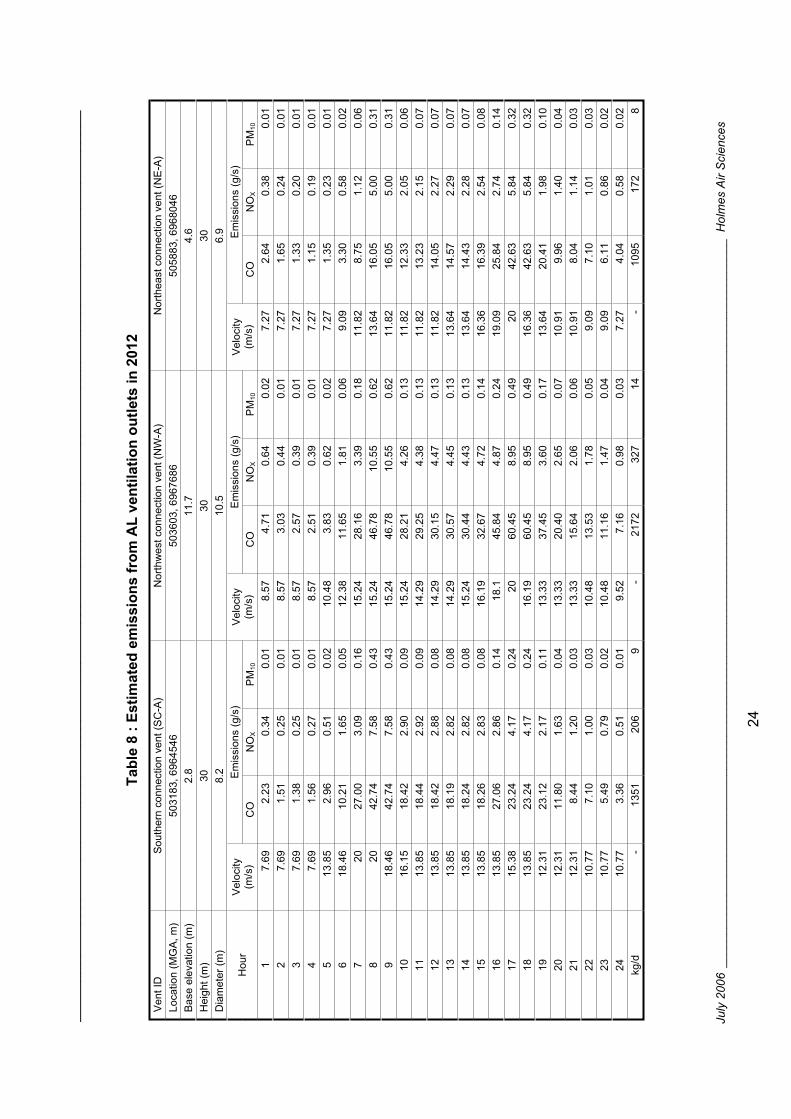
____
____
____
____
____
____
____
____
____
____
____
____
____
____
____
____
____
____
____
____
____
____
____
____
____
____
____
____
July
200
6__
____
____
____
____
____
____
____
____
____
____
____
____
____
____
____
____
____
____
____
____
____
____
____
____
____
____
____
Hol
mes
Air
Sci
ence
s
24
Tabl
e 8
: Est
imat
ed e
mis
sion
s fr
om A
L ve
ntila
tion
outle
ts in
201
2V
ent I
D
Sou
ther
n co
nnec
tion
vent
(SC
-A)
Nor
thw
est c
onne
ctio
n ve
nt (N
W-A
) N
orth
east
con
nect
ion
vent
(NE
-A)
Loca
tion
(MG
A, m
) 50
3183
, 696
4546
50
3603
, 696
7686
50
5883
, 696
8046
B
ase
elev
atio
n (m
) 2.
8 11
.7
4.6
Hei
ght (
m)
30
30
30
Dia
met
er (m
) 8.
2 10
.5
6.9
Em
issi
ons
(g/s
) E
mis
sion
s (g
/s)
Em
issi
ons
(g/s
) H
our
Vel
ocity
(m
/s)
CO
N
OX
PM
10
Vel
ocity
(m
/s)
CO
N
OX
PM
10
Vel
ocity
(m
/s)
CO
N
OX
PM
10
1 7.
69
2.23
0.
34
0.01
8.
57
4.71
0.
64
0.02
7.
27
2.64
0.
38
0.01
2
7.69
1.
51
0.25
0.
01
8.57
3.
03
0.44
0.
01
7.27
1.
65
0.24
0.
01
3 7.
69
1.38
0.
25
0.01
8.
57
2.57
0.
39
0.01
7.
27
1.33
0.
20
0.01
4
7.69
1.
56
0.27
0.
01
8.57
2.
51
0.39
0.
01
7.27
1.
15
0.19
0.
01
5 13
.85
2.96
0.
51
0.02
10
.48
3.83
0.
62
0.02
7.
27
1.35
0.
23
0.01
6
18.4
6 10
.21
1.65
0.
05
12.3
8 11
.65
1.81
0.
06
9.09
3.
30
0.58
0.
02
7 20
27
.00
3.09
0.
16
15.2
4 28
.16
3.39
0.
18
11.8
2 8.
75
1.12
0.
06
8 20
42
.74
7.58
0.
43
15.2
4 46
.78
10.5
5 0.
62
13.6
4 16
.05
5.00
0.
31
9 18
.46
42.7
4 7.
58
0.43
15
.24
46.7
8 10
.55
0.62
11
.82
16.0
5 5.
00
0.31
10
16
.15
18.4
2 2.
90
0.09
15
.24
28.2
1 4.
26
0.13
11
.82
12.3
3 2.
05
0.06
11
13
.85
18.4
4 2.
92
0.09
14
.29
29.2
5 4.
38
0.13
11
.82
13.2
3 2.
15
0.07
12
13
.85
18.4
2 2.
88
0.08
14
.29
30.1
5 4.
47
0.13
11
.82
14.0
5 2.
27
0.07
13
13
.85
18.1
9 2.
82
0.08
14
.29
30.5
7 4.
45
0.13
13
.64
14.5
7 2.
29
0.07
14
13
.85
18.2
4 2.
82
0.08
15
.24
30.4
4 4.
43
0.13
13
.64
14.4
3 2.
28
0.07
15
13
.85
18.2
6 2.
83
0.08
16
.19
32.6
7 4.
72
0.14
16
.36
16.3
9 2.
54
0.08
16
13
.85
27.0
6 2.
86
0.14
18
.1
45.8
4 4.
87
0.24
19
.09
25.8
4 2.
74
0.14
17
15
.38
23.2
4 4.
17
0.24
20
60
.45
8.95
0.
49
20
42.6
3 5.
84
0.32
18
13
.85
23.2
4 4.
17
0.24
16
.19
60.4
5 8.
95
0.49
16
.36
42.6
3 5.
84
0.32
19
12
.31
23.1
2 2.
17
0.11
13
.33
37.4
5 3.
60
0.17
13
.64
20.4
1 1.
98
0.10
20
12
.31
11.8
0 1.
63
0.04
13
.33
20.4
0 2.
65
0.07
10
.91
9.96
1.
40
0.04
21
12
.31
8.44
1.
20
0.03
13
.33
15.6
4 2.
06
0.06
10
.91
8.04
1.
14
0.03
22
10
.77
7.10
1.
00
0.03
10
.48
13.5
3 1.
78
0.05
9.
09
7.10
1.
01
0.03
23
10
.77
5.49
0.
79
0.02
10
.48
11.1
6 1.
47
0.04
9.
09
6.11
0.
86
0.02
24
10
.77
3.36
0.
51
0.01
9.
52
7.16
0.
98
0.03
7.
27
4.04
0.
58
0.02
kg
/d
- 13
51
206
9 -
2172
32
7 14
-
1095
17
2 8
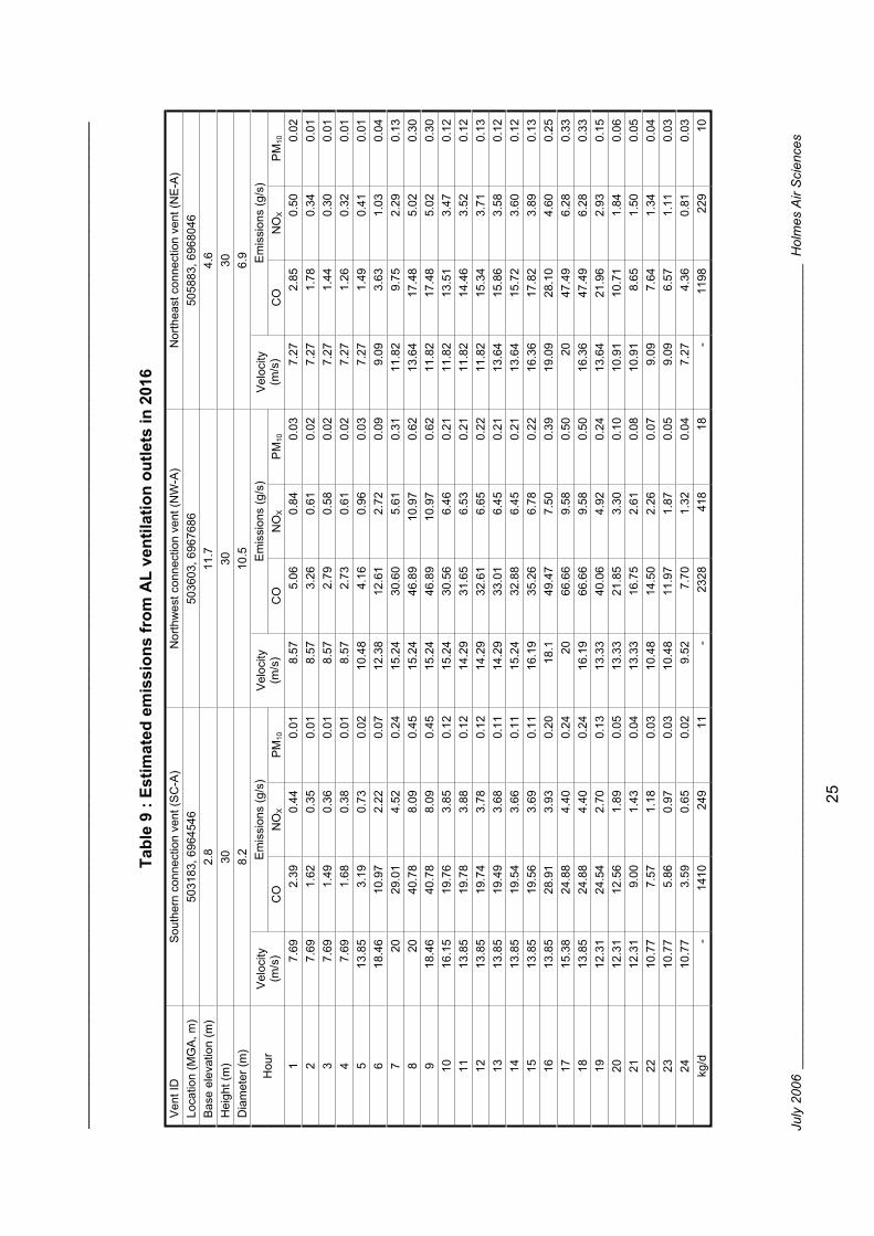
____
____
____
____
____
____
____
____
____
____
____
____
____
____
____
____
____
____
____
____
____
____
____
____
____
____
____
____
July
200
6__
____
____
____
____
____
____
____
____
____
____
____
____
____
____
____
____
____
____
____
____
____
____
____
____
____
____
____
Hol
mes
Air
Sci
ence
s
25
Tabl
e 9
: Est
imat
ed e
mis
sion
s fr
om A
L ve
ntila
tion
outle
ts in
201
6 V
ent I
D
Sou
ther
n co
nnec
tion
vent
(SC
-A)
Nor
thw
est c
onne
ctio
n ve
nt (N
W-A
) N
orth
east
con
nect
ion
vent
(NE
-A)
Loca
tion
(MG
A, m
) 50
3183
, 696
4546
50
3603
, 696
7686
50
5883
, 696
8046
B
ase
elev
atio
n (m
) 2.
8 11
.7
4.6
Hei
ght (
m)
30
30
30
Dia
met
er (m
) 8.
2 10
.5
6.9
Em
issi
ons
(g/s
) E
mis
sion
s (g
/s)
Em
issi
ons
(g/s
) H
our
Vel
ocity
(m
/s)
CO
N
OX
PM
10
Vel
ocity
(m
/s)
CO
N
OX
PM
10
Vel
ocity
(m
/s)
CO
N
OX
PM
10
1 7.
69
2.39
0.
44
0.01
8.
57
5.06
0.
84
0.03
7.
27
2.85
0.
50
0.02
2
7.69
1.
62
0.35
0.
01
8.57
3.
26
0.61
0.
02
7.27
1.
78
0.34
0.
01
3 7.
69
1.49
0.
36
0.01
8.
57
2.79
0.
58
0.02
7.
27
1.44
0.
30
0.01
4
7.69
1.
68
0.38
0.
01
8.57
2.
73
0.61
0.
02
7.27
1.
26
0.32
0.
01
5 13
.85
3.19
0.
73
0.02
10
.48
4.16
0.
96
0.03
7.
27
1.49
0.
41
0.01
6
18.4
6 10
.97
2.22
0.
07
12.3
8 12
.61
2.72
0.
09
9.09
3.
63
1.03
0.
04
7 20
29
.01
4.52
0.
24
15.2
4 30
.60
5.61
0.
31
11.8
2 9.
75
2.29
0.
13
8 20
40
.78
8.09
0.
45
15.2
4 46
.89
10.9
7 0.
62
13.6
4 17
.48
5.02
0.
30
9 18
.46
40.7
8 8.
09
0.45
15
.24
46.8
9 10
.97
0.62
11
.82
17.4
8 5.
02
0.30
10
16
.15
19.7
6 3.
85
0.12
15
.24
30.5
6 6.
46
0.21
11
.82
13.5
1 3.
47
0.12
11
13
.85
19.7
8 3.
88
0.12
14
.29
31.6
5 6.
53
0.21
11
.82
14.4
6 3.
52
0.12
12
13
.85
19.7
4 3.
78
0.12
14
.29
32.6
1 6.
65
0.22
11
.82
15.3
4 3.
71
0.13
13
13
.85
19.4
9 3.
68
0.11
14
.29
33.0
1 6.
45
0.21
13
.64
15.8
6 3.
58
0.12
14
13
.85
19.5
4 3.
66
0.11
15
.24
32.8
8 6.
45
0.21
13
.64
15.7
2 3.
60
0.12
15
13
.85
19.5
6 3.
69
0.11
16
.19
35.2
6 6.
78
0.22
16
.36
17.8
2 3.
89
0.13
16
13
.85
28.9
1 3.
93
0.20
18
.1
49.4
7 7.
50
0.39
19
.09
28.1
0 4.
60
0.25
17
15
.38
24.8
8 4.
40
0.24
20
66
.66
9.58
0.
50
20
47.4
9 6.
28
0.33
18
13
.85
24.8
8 4.
40
0.24
16
.19
66.6
6 9.
58
0.50
16
.36
47.4
9 6.
28
0.33
19
12
.31
24.5
4 2.
70
0.13
13
.33
40.0
6 4.
92
0.24
13
.64
21.9
6 2.
93
0.15
20
12
.31
12.5
6 1.
89
0.05
13
.33
21.8
5 3.
30
0.10
10
.91
10.7
1 1.
84
0.06
21
12
.31
9.00
1.
43
0.04
13
.33
16.7
5 2.
61
0.08
10
.91
8.65
1.
50
0.05
22
10
.77
7.57
1.
18
0.03
10
.48
14.5
0 2.
26
0.07
9.
09
7.64
1.
34
0.04
23
10
.77
5.86
0.
97
0.03
10
.48
11.9
7 1.
87
0.05
9.
09
6.57
1.
11
0.03
24
10
.77
3.59
0.
65
0.02
9.
52
7.70
1.
32
0.04
7.
27
4.36
0.
81
0.03
kg
/d
- 14
10
249
11
- 23
28
418
18
- 11
98
229
10
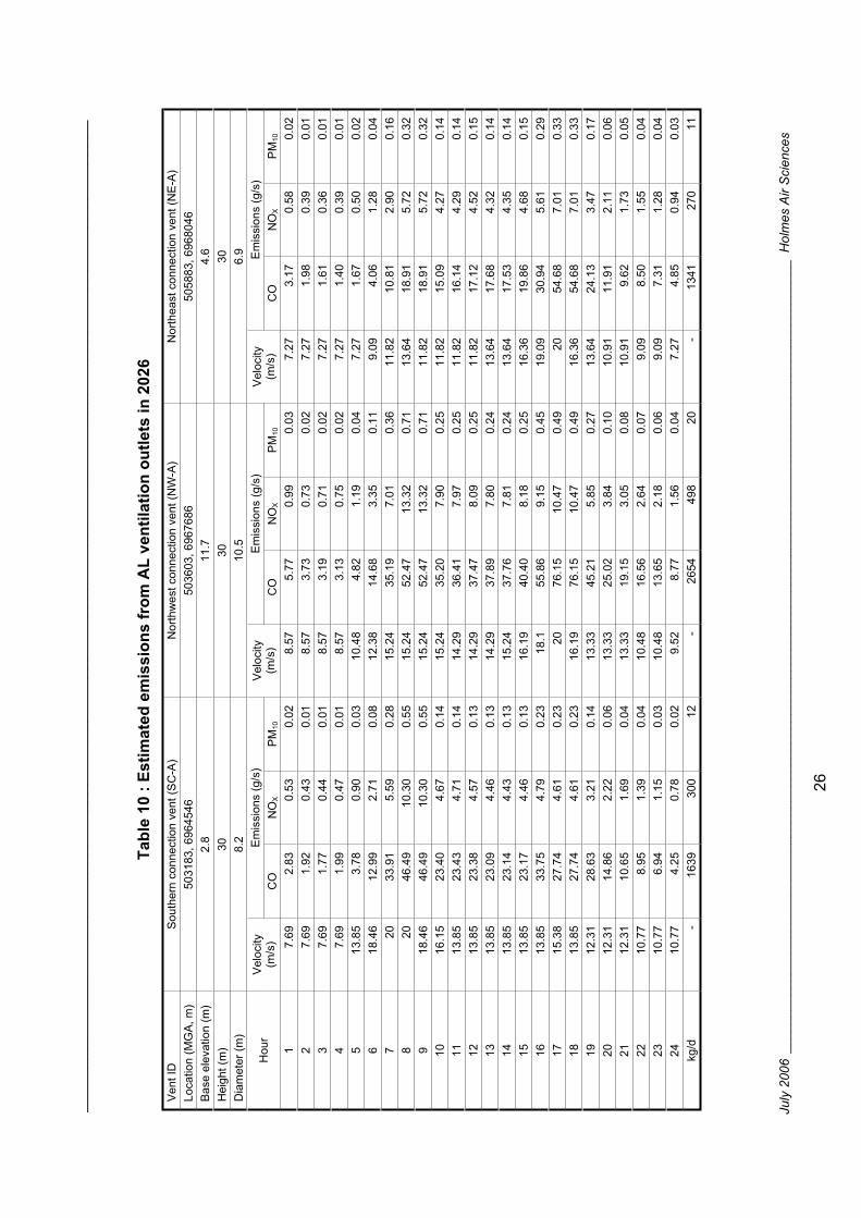
____
____
____
____
____
____
____
____
____
____
____
____
____
____
____
____
____
____
____
____
____
____
____
____
____
____
____
____
July
200
6__
____
____
____
____
____
____
____
____
____
____
____
____
____
____
____
____
____
____
____
____
____
____
____
____
____
____
____
Hol
mes
Air
Sci
ence
s
26
Tabl
e 10
: Es
timat
ed e
mis
sion
s fr
om A
L ve
ntila
tion
outle
ts in
202
6 V
ent I
D
Sou
ther
n co
nnec
tion
vent
(SC
-A)
Nor
thw
est c
onne
ctio
n ve
nt (N
W-A
) N
orth
east
con
nect
ion
vent
(NE
-A)
Loca
tion
(MG
A, m
) 50
3183
, 696
4546
50
3603
, 696
7686
50
5883
, 696
8046
B
ase
elev
atio
n (m
) 2.
8 11
.7
4.6
Hei
ght (
m)
30
30
30
Dia
met
er (m
) 8.
2 10
.5
6.9
Em
issi
ons
(g/s
) E
mis
sion
s (g
/s)
Em
issi
ons
(g/s
) H
our
Vel
ocity
(m
/s)
CO
N
OX
PM
10
Vel
ocity
(m
/s)
CO
N
OX
PM
10
Vel
ocity
(m
/s)
CO
N
OX
PM
10
1 7.
69
2.83
0.
53
0.02
8.
57
5.77
0.
99
0.03
7.
27
3.17
0.
58
0.02
2
7.69
1.
92
0.43
0.
01
8.57
3.
73
0.73
0.
02
7.27
1.
98
0.39
0.
01
3 7.
69
1.77
0.
44
0.01
8.
57
3.19
0.
71
0.02
7.
27
1.61
0.
36
0.01
4
7.69
1.
99
0.47
0.
01
8.57
3.
13
0.75
0.
02
7.27
1.
40
0.39
0.
01
5 13
.85
3.78
0.
90
0.03
10
.48
4.82
1.
19
0.04
7.
27
1.67
0.
50
0.02
6
18.4
6 12
.99
2.71
0.
08
12.3
8 14
.68
3.35
0.
11
9.09
4.
06
1.28
0.
04
7 20
33
.91
5.59
0.
28
15.2
4 35
.19
7.01
0.
36
11.8
2 10
.81
2.90
0.
16
8 20
46
.49
10.3
0 0.
55
15.2
4 52
.47
13.3
2 0.
71
13.6
4 18
.91
5.72
0.
32
9 18
.46
46.4
9 10
.30
0.55
15
.24
52.4
7 13
.32
0.71
11
.82
18.9
1 5.
72
0.32
10
16
.15
23.4
0 4.
67
0.14
15
.24
35.2
0 7.
90
0.25
11
.82
15.0
9 4.
27
0.14
11
13
.85
23.4
3 4.
71
0.14
14
.29
36.4
1 7.
97
0.25
11
.82
16.1
4 4.
29
0.14
12
13
.85
23.3
8 4.
57
0.13
14
.29
37.4
7 8.
09
0.25
11
.82
17.1
2 4.
52
0.15
13
13
.85
23.0
9 4.
46
0.13
14
.29
37.8
9 7.
80
0.24
13
.64
17.6
8 4.
32
0.14
14
13
.85
23.1
4 4.
43
0.13
15
.24
37.7
6 7.
81
0.24
13
.64
17.5
3 4.
35
0.14
15
13
.85
23.1
7 4.
46
0.13
16
.19
40.4
0 8.
18
0.25
16
.36
19.8
6 4.
68
0.15
16
13
.85
33.7
5 4.
79
0.23
18
.1
55.8
6 9.
15
0.45
19
.09
30.9
4 5.
61
0.29
17
15
.38
27.7
4 4.
61
0.23
20
76
.15
10.4
7 0.
49
20
54.6
8 7.
01
0.33
18
13
.85
27.7
4 4.
61
0.23
16
.19
76.1
5 10
.47
0.49
16
.36
54.6
8 7.
01
0.33
19
12
.31
28.6
3 3.
21
0.14
13
.33
45.2
1 5.
85
0.27
13
.64
24.1
3 3.
47
0.17
20
12
.31
14.8
6 2.
22
0.06
13
.33
25.0
2 3.
84
0.10
10
.91
11.9
1 2.
11
0.06
21
12
.31
10.6
5 1.
69
0.04
13
.33
19.1
5 3.
05
0.08
10
.91
9.62
1.
73
0.05
22
10
.77
8.95
1.
39
0.04
10
.48
16.5
6 2.
64
0.07
9.
09
8.50
1.
55
0.04
23
10
.77
6.94
1.
15
0.03
10
.48
13.6
5 2.
18
0.06
9.
09
7.31
1.
28
0.04
24
10
.77
4.25
0.
78
0.02
9.
52
8.77
1.
56
0.04
7.
27
4.85
0.
94
0.03
kg
/d
- 16
39
300
12
- 26
54
498
20
- 13
41
270
11
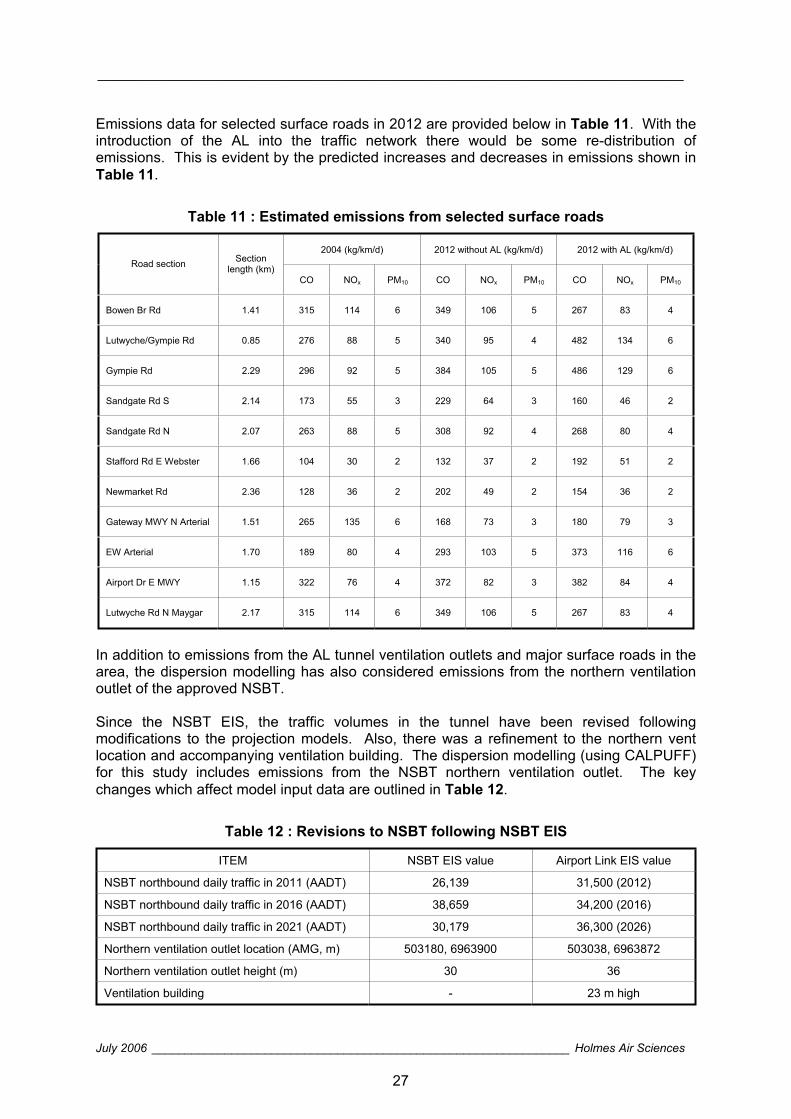
________________________________________________________________________
July 2006 _______________________________________________________________ Holmes Air Sciences
27
Emissions data for selected surface roads in 2012 are provided below in Table 11. With the introduction of the AL into the traffic network there would be some re-distribution of emissions. This is evident by the predicted increases and decreases in emissions shown in Table 11.
Table 11 : Estimated emissions from selected surface roads
2004 (kg/km/d) 2012 without AL (kg/km/d) 2012 with AL (kg/km/d) Road section Section
length (km) CO NOx PM10 CO NOx PM10 CO NOx PM10
Bowen Br Rd 1.41 315 114 6 349 106 5 267 83 4
Lutwyche/Gympie Rd 0.85 276 88 5 340 95 4 482 134 6
Gympie Rd 2.29 296 92 5 384 105 5 486 129 6
Sandgate Rd S 2.14 173 55 3 229 64 3 160 46 2
Sandgate Rd N 2.07 263 88 5 308 92 4 268 80 4
Stafford Rd E Webster 1.66 104 30 2 132 37 2 192 51 2
Newmarket Rd 2.36 128 36 2 202 49 2 154 36 2
Gateway MWY N Arterial 1.51 265 135 6 168 73 3 180 79 3
EW Arterial 1.70 189 80 4 293 103 5 373 116 6
Airport Dr E MWY 1.15 322 76 4 372 82 3 382 84 4
Lutwyche Rd N Maygar 2.17 315 114 6 349 106 5 267 83 4
In addition to emissions from the AL tunnel ventilation outlets and major surface roads in the area, the dispersion modelling has also considered emissions from the northern ventilation outlet of the approved NSBT.
Since the NSBT EIS, the traffic volumes in the tunnel have been revised following modifications to the projection models. Also, there was a refinement to the northern vent location and accompanying ventilation building. The dispersion modelling (using CALPUFF) for this study includes emissions from the NSBT northern ventilation outlet. The key changes which affect model input data are outlined in Table 12.
Table 12 : Revisions to NSBT following NSBT EIS
ITEM NSBT EIS value Airport Link EIS value
NSBT northbound daily traffic in 2011 (AADT) 26,139 31,500 (2012)
NSBT northbound daily traffic in 2016 (AADT) 38,659 34,200 (2016)
NSBT northbound daily traffic in 2021 (AADT) 30,179 36,300 (2026)
Northern ventilation outlet location (AMG, m) 503180, 6963900 503038, 6963872
Northern ventilation outlet height (m) 30 36
Ventilation building - 23 m high

________________________________________________________________________
July 2006 _______________________________________________________________ Holmes Air Sciences
28
Pollutant emissions from the NSBT northern ventilation outlet have been scaled from the EIS estimates according to the modifications to AADT in the northbound tunnel.
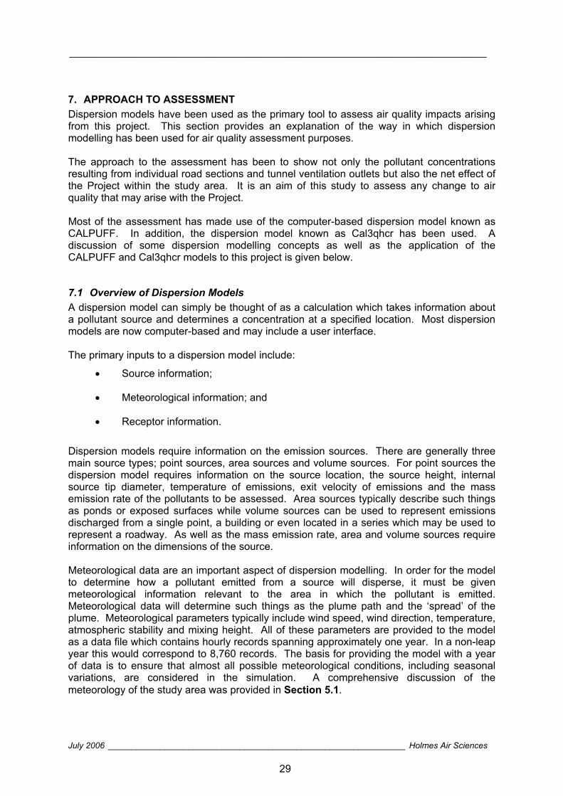
________________________________________________________________________
July 2006 _______________________________________________________________ Holmes Air Sciences
29
7. APPROACH TO ASSESSMENT Dispersion models have been used as the primary tool to assess air quality impacts arising from this project. This section provides an explanation of the way in which dispersion modelling has been used for air quality assessment purposes.
The approach to the assessment has been to show not only the pollutant concentrations resulting from individual road sections and tunnel ventilation outlets but also the net effect of the Project within the study area. It is an aim of this study to assess any change to air quality that may arise with the Project.
Most of the assessment has made use of the computer-based dispersion model known as CALPUFF. In addition, the dispersion model known as Cal3qhcr has been used. A discussion of some dispersion modelling concepts as well as the application of the CALPUFF and Cal3qhcr models to this project is given below.
7.1 Overview of Dispersion Models A dispersion model can simply be thought of as a calculation which takes information about a pollutant source and determines a concentration at a specified location. Most dispersion models are now computer-based and may include a user interface.
The primary inputs to a dispersion model include:
Source information;
Meteorological information; and
Receptor information.
Dispersion models require information on the emission sources. There are generally three main source types; point sources, area sources and volume sources. For point sources the dispersion model requires information on the source location, the source height, internal source tip diameter, temperature of emissions, exit velocity of emissions and the mass emission rate of the pollutants to be assessed. Area sources typically describe such things as ponds or exposed surfaces while volume sources can be used to represent emissions discharged from a single point, a building or even located in a series which may be used to represent a roadway. As well as the mass emission rate, area and volume sources require information on the dimensions of the source.
Meteorological data are an important aspect of dispersion modelling. In order for the model to determine how a pollutant emitted from a source will disperse, it must be given meteorological information relevant to the area in which the pollutant is emitted. Meteorological data will determine such things as the plume path and the ‘spread’ of the plume. Meteorological parameters typically include wind speed, wind direction, temperature, atmospheric stability and mixing height. All of these parameters are provided to the model as a data file which contains hourly records spanning approximately one year. In a non-leap year this would correspond to 8,760 records. The basis for providing the model with a year of data is to ensure that almost all possible meteorological conditions, including seasonal variations, are considered in the simulation. A comprehensive discussion of the meteorology of the study area was provided in Section 5.1.
________________________________________________________________________
July 2006 _______________________________________________________________ Holmes Air Sciences
30
Receptor information is defined by the user and relates to the locations for which predictions of pollutant concentrations are required. Usually the location of receptors are defined at ground-level, where most people reside, however it is also possible to set a receptor at a location above ground. Examples of above-ground or elevated receptors are air intake points on a building.
The calculations within a dispersion model are organised in a series of loops. The first step the model takes is usually to read one hour of meteorological information. Then, in the case of a single source, the model will determine the plume structure and then calculate the resultant pollutant concentration at every receptor specified by the user. Following these calculations the model reads the next hour of meteorological information and the process repeats itself until all hours in the meteorological file have been read. During the simulation the calculations are stored in the computer’s memory and once the model run is complete, statistics such as pollutant maxima and averages can be retrieved.
The units of measurement for pollutant mass emission rates are different from the units of measurement for pollutant concentration and may sometimes cause some confusion. Mass emission rate defines the pollutant mass by time (for example, grams per second) while concentration defines the pollutant by volume; grams per cubic metre for example. Air quality goals are generally specified as a concentration.
It should be mentioned that air dispersion models can be classed as being one of two types; a steady-state model or a non steady-state model. A thorough description of the differences between the two model types is not necessary for the purposes of this report, however, it is useful to note that the fundamental difference relates to the simulated plume behaviour.
Steady-state models essentially create a plume which extends to infinity downwind. Once the next hour of meteorological data is read a new plume is created and memory of the plume in the previous hour is lost.
Non steady-state models allow the plume to grow and bend with differences in meteorology over the modelling area. Unlike steady-state models these types of models have a ‘memory’ of the plume for the previous hours. The concept of non steady-state is considered to be a more realistic simulation of plume behaviour than that provided by steady-state models.
7.2 CALMET and CALPUFF The CALMET/CALPUFF modelling system is considered to be one of the most sophisticated models available. CALPUFF is an advanced computer-based dispersion model that simulates the dispersion of emissions by representing emissions as a series of puffs emitted sequentially. Provided the rate at which the puffs are emitted is sufficiently rapid, the puffs will overlap and the serial release will represent a continuous release.
The advantage of the puff modelling approach over the steady state Gaussian models such as ISCST3 and AUSPLUME, which have also been widely used in source dispersion assessments in the past, is that the progress and dispersion of each individual puff can be treated separately and can be made to account for local wind conditions and the way in which wind conditions at a particular place vary with time.
The CALPUFF model has been chosen as the primary tool for the purposes of this assessment. The main purpose of the CALPUFF modelling is to simulate the air quality impacts of the Project on a regional scale (approximately 20 km by 20 km area) and to show the net effect of introducing the tunnel into the area. The traffic information (see Section6.2) reveals that the introduction of a tunnel into the Brisbane area will change traffic
________________________________________________________________________
July 2006 _______________________________________________________________ Holmes Air Sciences
31
volumes on many of the region’s roads. These changes may either be increases or decreases in total traffic volumes. Some roads, such as minor residential roads, are expected to experience little change in traffic volumes. The CALPUFF modelling seeks to simulate these effects.
On the regional scale the pollutant emission sources have been divided into three categories:
1. Ventilation outlets associated with the tunnel
2. Roads generally carrying greater than 20,000 vehicles per day (AADT)
3. Roads generally carrying less than 20,000 vehicles per day (AADT)
Ventilation outlets associated with the tunnel have been represented as point sources in the dispersion model. Source locations, source characteristics and hourly variable pollutant emissions are provided to the model in the form of an external emissions file. Details of emissions from each outlet have been discussed in Section 6.3. Where known, buildings in the vicinity of the ventilation outlets which would influence plume behaviour have been included in the modelling and the PRIME building wake algorithm has been selected.
Roads carrying greater than 20,000 vehicles per day have also been explicitly included as sources in the model. Each road meeting this traffic volume criteria has been represented as a series of volume sources over the length of the road section. Each volume source has a location, elevation, height above ground and two additional parameters relating to the size of the source in the horizontal and vertical planes. Pollutant emissions are modelled to vary by hour of day for every volume source representing part of a road section. Figure 17shows the location of all volume sources which have been used to represent roads in the CALPUFF simulations.
It is technically possible to include all other minor roads with known traffic volume in the study area into the model however an alternate approach has been taken in this study to account for these sources. Roads carrying less than 20,000 vehicles per day have been accounted for by adding to the simulation the hourly varying ambient air quality monitoring data. For this approach it was necessary to construct a file for each modelled pollutant which contains hourly records of ambient pollutant concentrations based on the air quality monitoring. The ‘background’ data files have been constructed from EPA air quality monitoring data, specifically, Eagle Farm.
In the case of CO and NOx, emissions contributing to the EPA air quality monitoring data in the Brisbane area would be mainly from motor vehicles. It would therefore be considered appropriate to use an hourly background file to represent the non-modelled roads, that is, roads carrying less than about 20,000 vehicles per day. To create the background files for CO and NOx, it is also appropriate to use data from a site which may be least influenced by high trafficked roads. Eagle Farm is considered to be a suitable site for this objective, rather than city-based monitoring sites.
An hourly background NO2 data file has been created from the Eagle Farm air quality monitoring data. In order to create an hourly background CO data file, the likely CO concentrations at Eagle Farm have been derived from the relationship between CO and NOXconcentrations at the South Brisbane site (Holmes Air Sciences, 2004). Figure 18 shows the almost linear relationship between hourly CO and NOx concentrations.
There are many sources of particulate matter in the Brisbane area that would contribute to the measurements reported in the EPA monitoring data. These sources may include
________________________________________________________________________
July 2006 _______________________________________________________________ Holmes Air Sciences
32
bushfires, construction activities and sea salt in addition to motor vehicle emissions. Using a background particulate matter data file to represent emissions from non-modelled roads would therefore not be appropriate in this instance. The approach adopted for particulate matter was to show the predicted contribution of the modelled sources alone and to determine if there would be any additional exceedances of the air quality criteria.
The modelling has been performed using the meteorological information provided by the CALMET model (Section 5.1) and the emissions information summarised in Section 6.3.
The CALPUFF model simulations include the following scenarios:
2004, existing case. Used for model performance analysis and comparison with future scenarios;
2012. Intended year for tunnel opening;
2016. Five years after intended year for tunnel opening; and
2026. Fourteen years after intended year for tunnel opening.
In addition, “do minimal” (no tunnel) scenarios for 2012, 2016 and 2026 have been modelled and form a key component to the assessment.
Predictions were made over a large set of ground-level discrete receptors arranged in the study area. Spacing between receptors was set finer in areas closer to sources and coarser in areas further from sources. The receptor spacing and locations have been chosen to provide high resolution model output where needed.
7.3 Cal3qhcr The CALINE series of dispersion models has been widely used in roadway studies throughout Australia to estimate pollutant concentrations close to roadways. The models are steady-state dispersion models which can determine concentrations at receptor locations downwind of “at grade”, “fill”, “bridges” and “cut section” highways located in relatively uncomplicated terrain. The models are applicable for most wind directions, highway orientations and receptor locations.
Cal3qhcr is one of a number of models in the CALINE series and is an enhancement of the Cal3qhc and Caline-3 roadway models to allow real (long-term) meteorological data. Model inputs also include roadway geometries, receptor locations and vehicular emission rates. The model is suitable for predictions within a few hundred metres of the roadway. Further details on the CALINE models can be found in the user manuals (US EPA website).
The main purpose of the Cal3qhcr modelling is to assess air quality impacts very close to selected roadways resulting from changes to lane configurations and traffic volumes. Although the CALPUFF model can simulate the dispersion of emissions from both line sources and point sources, it was not specifically designed for roadway emissions. In practice CALPUFF does not take account of the dispersion close to the road, where vehicle induced turbulence has significant influence. The CALINE models simulate this turbulence better than CALPUFF.
________________________________________________________________________
July 2006 _______________________________________________________________ Holmes Air Sciences
33
Eleven surface roadways have been selected for analysis using the Cal3qhcr model. These surface roadways are:
Bowen Bridge Road
Lutwyche/Gympie Road
Gympie Road
Sandgate Road, south of East-West Arterial Road
Sandgate Road, north of East-West Arterial Road
Stafford Road, east of Webster Street
Newmarket Road
Gateway Motorway, north of Airport Drive
East-West Arterial Road
Airport Drive
Lutwyche Road north of Maygar Street
Figure 19 shows the location of these road sections.
________________________________________________________________________
July 2006 _______________________________________________________________ Holmes Air Sciences
34
8. ASSESSMENT OF AIR QUALITY IMPACTS This section provides an assessment of the air quality impacts associated with the Project. Some of the questions which are attempted to be answered in this discussion include:
How would air quality change as a result of the Project?
How do the air quality impacts of the Project compare with the “do nothing” case?
What are the pollutant contributions from ventilation outlets and surface roads?
There are many figures accompanying this report which present the results of the dispersion modelling. The quantity of figures has arisen from the requirement to address many different pollutants, future years and build or no-build cases and to ensure that any possible adverse air quality impacts are not overlooked. It is possible, however, to observe the overall air quality impacts of the Project just by reviewing predictions for one pollutant only as similar trends for different pollutants have been noted.
All dispersion model results directly reflect the modelled traffic volumes for the Project.
8.1 Regional Effects Figures 20 to 39 have been created from the dispersion modelling results in order to show the effect of the Project (in terms of air quality impacts) at a regional scale. The region defined for these results covers an area 17 km by 12 km. The figures attempt to show the likely pollutant concentrations in the study area arising from sources which include surface roads and tunnel ventilation outlets (in cases where applicable).
The results for regional effects (Figures 20 to 39) are grouped by criteria pollutants, averaging time and years. Table 13 has been created to assist with referencing the figures.
Table 13 : Quick reference to dispersion model results figure number
SimulationPollutant and averaging time case 2004
2012
(DS & DM)
2016
(DS & DM)
2026
(DS & DM)
Maximum 8-hour average CO Figure 20 Figure 21 Figure 22 Figure 23
Maximum 1-hour average NO2 Figure 24 Figure 25 Figure 26 Figure 27
Annual average NO2 Figure 28 Figure 29 Figure 30 Figure 31
Maximum 24-hour average PM10 Figure 32 Figure 33 Figure 34 Figure 35
Annual average PM10 Figure 36 Figure 37 Figure 38 Figure 39
It should be noted that predictions for maximum levels (that is, maximum 1-hour, 8-hour and 24-hour averages) do not show the dispersion pattern at any one point in time but show the maximum levels that occurred at each location over the entire meteorological dataset. Annual average prediction plots simply show the average levels for each location.
In addition to the results presented as absolute pollutant concentrations, Figures 41 to 45have been developed to compare the existing situation with future (2012) with and without
________________________________________________________________________
July 2006 _______________________________________________________________ Holmes Air Sciences
35
tunnel cases. These results are presented as a percentage change in pollutant concentrations.
Comments on the dispersion model results for each of the criteria pollutants are provided below.
Carbon Monoxide The simulations of CO concentrations in the study area (Figures 20 to 23) include surface road sources and tunnel ventilation outlets where appropriate. Background CO concentrations are also included in these predictions.
The first figure in the series of CO plots (Figure 20) shows the predictions for 2004. The 2004 simulation can be considered to represent the modelled “existing” situation. Following 2004 are the 2012, 2016 and 2026 simulations which include the build and no-build cases. This grouping pattern is maintained for all pollutants.
The following observations were made from the review of the CO model predictions:
Predictions for the existing case (2004) show that maximum 8-hour average CO concentrations are below the 8-hour maximum air quality goal of 10 mg/m3. The air quality monitoring data also shows that existing maximum 8-hour average CO concentrations are below 10 mg/m3.
CO concentrations in future years (2012+) are predicted to be very similar to existing (2004) concentrations. The likely improvements to vehicle emissions appear to offset projected increases in traffic in the study area. However, the emission estimates have not considered any further tightening of emission standards so the future projections are considered to be conservative.
As expected, higher CO concentrations are predicted near roads carrying more traffic.
Predictions for the future (2012+) build and no-build cases are very similar.
The contribution to ground-level concentrations due to tunnel ventilation outlets (with AL case) appear to be overwhelmed by contributions from the major surface roads.
Nitrogen Dioxide Predictions of NO2 concentrations in the study area for existing and future years present a similar story to the CO predictions. These results (Figures 24 to 31) also include background NO2 concentrations.
The following observations were made from the review of the NO2 model predictions:
Predictions for the existing case (2004) show that maximum 1-hour average NO2
concentrations are up to around 200 g/m3 near the busy roads in the CBD.These levels are below the 246 g/m3 air quality goal. Monitoring data from the sites examined for this study (that is, Bowen Hills, Eagle Farm and Kedron) show that existing maximum 1-hour average NO2 concentrations are below the goal.
Predictions for the existing case (2004) show that annual average NO2
concentrations are below the annual air quality goal of 62 g/m3. The air quality monitoring data also shows that existing annual average NO2 concentrations are below 62 g/m3.
________________________________________________________________________
July 2006 _______________________________________________________________ Holmes Air Sciences
36
NO2 concentrations in future years (2012+) are predicted to be very similar to existing (2004) concentrations. The likely improvements to vehicle emissions appear to offset projected increases in traffic in the study area. However, the emission estimates have not considered any further tightening of emission standards so the future projections are considered to be conservative.
As expected, higher NO2 concentrations are predicted near roads carrying more traffic.
Predictions for the future (2012+) build and no-build cases are very similar.
The contribution to ground-level concentrations due to tunnel ventilation outlets (with AL case) appear to be overwhelmed by contributions from the major surface roads.
Particulate Matter (PM10 and PM2.5)Figures 32 to 39 present the regional dispersion modelling results for PM10. The most stringent PM10 air quality goals from Table 1 are 50 g/m3 and 30 g/m3 for maximum 24-hour and annual averages respectively. Review of the air quality monitoring data for the study area (Section 5.4) showed that existing maximum 24-hour background PM10 levels can be above 50 g/m3 (up to 85 g/m3) and the major sources contributing to these levels are most likely bushfires and dust storms. For this reason the concentrations shown in the PM10 plots include only the modelled surface roads and ventilation outlet sources.
As for CO and NO2, there are some common patterns of high and low concentrations predicted in the study area resulting from the modelled sources. The dispersion model predictions for PM10 are summarised below:
Predictions for the existing case (2004) show that PM10 concentrations are below the maximum 24-hour and annual average air quality goals (50 and 30 g/m3)however these predictions are due only to the modelled sources and not events such as bushfires.
PM10 concentrations in future years (2012+) are predicted to very similar to existing (2004) concentrations. The likely improvements to vehicle emissions appear to offset projected increases in traffic in the study area. Again, the emission estimates have not considered any further tightening of emission standards so the future projections are considered to be conservative.
Higher PM10 concentrations are predicted near roads carrying more traffic.
Predictions for the future (2012+) build and no-build cases are very similar.
The contribution to ground-level concentrations due to tunnel ventilation outlets (with AL case) appear to be overwhelmed by contributions from the major surface roads.
There is a widely held view that the majority of PM10 is PM2.5 from motor vehicles however some monitoring data for tunnel projects indicate otherwise. For example, monitoring in the tunnel outlet for the M5-East tunnel in Sydney shows that about 35% of the PM10 is PM2.5,while for the CityLink tunnel in Melbourne, tunnel outlet monitoring shows that about 70% of the PM10 is PM2.5.
Monitoring data from Bowen Hills shows that 50% of the PM10 is PM2.5 although this fraction is relevant for ambient particulate matter concentrations. Actual percentages of PM2.5 in the
________________________________________________________________________
July 2006 _______________________________________________________________ Holmes Air Sciences
37
PM10 from vehicle exhausts and tunnel ventilation outlets will vary, however, for the purposes of this study it has been conservatively assumed that 96% of the PM10 is PM2.5.This is based on measurements made in diesel exhaust (Environment Australia, 2003).Not all PM10 emissions from roadways are from diesel exhaust, they also include emissions from tyre and brake wear and emissions from petrol fuelled vehicles. Therefore, in practice the percentage will be less than 96%.
Model predictions for PM2.5 are shown in Figure 40. As discussed above these predictions take account of modelled surface roads and ventilation outlets where appropriate. No background levels have been included. By assuming that 96% of the PM10 is PM2.5, the changes in PM2.5 with and without the tunnel are relatively minor. As with PM10, the existing background levels already exceed the NEPM goal on occasions.
It is also worth noting that, in terms of total fine particulate loading, very clean environments such as Cape Grim on the north-western coast of Tasmania, which is a global baseline site, recorded average PM2.5 levels of 5.8 g/m3 from 2001 to 2003 compared to the NEPM goal of 8 g/m3 for fine particulate matter. This does not leave a large margin for compliance with the NEPM goal in urban areas. While the source of the particulate matter at Cape Grim is predominantly sea salt, the NEPM goal does not distinguish between fine particles of different chemical composition. Future air quality criteria may well incorporate the chemical nature of fine particles and ultrafine particles with the view that some particles are more harmful than others.
Table 14 presents the dispersion model results at selected locations in the study area for each of the criteria pollutants. From these results it is possible to assess the performance of the CALPUFF model, that is, by comparing the 2004 predictions with the 2004 monitoring data. Spatial variation (between the different sites) can also be assessed as well as differences between build and no-build cases and existing and future cases.
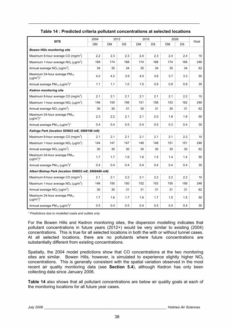
________________________________________________________________________
July 2006 _______________________________________________________________ Holmes Air Sciences
38
Table 14 : Predicted criteria pollutant concentrations at selected locations 2004 2012 2016 2026
SITEDM DM DS DM DS DM DS
Goal
Bowen Hills monitoring site
Maximum 8-hour average CO (mg/m3) 2.2 2.3 2.3 2.4 2.3 2.4 2.4 10
Maximum 1-hour average NO2 ( g/m3) 169 174 168 174 168 174 169 246
Annual average NO2 (ug/m3) 34 35 34 35 34 35 34 62
Maximum 24-hour average PM10
( g/m3)* 4.2 4.2 3.9 4.0 3.6 3.7 3.3 50
Annual average PM10 ( g/m3)* 1.1 1.1 1.0 1.0 0.9 0.9 0.8 30
Kedron monitoring site
Maximum 8-hour average CO (mg/m3) 2.1 2.1 2.1 2.1 2.1 2.1 2.2 10
Maximum 1-hour average NO2 ( g/m3) 146 150 156 151 158 153 162 246
Annual average NO2 (ug/m3) 30 30 31 30 31 30 31 62
Maximum 24-hour average PM10
( g/m3)* 2.3 2.2 2.1 2.1 2.0 1.8 1.8 50
Annual average PM10 ( g/m3)* 0.4 0.4 0.5 0.4 0.5 0.3 0.4 30
Kalinga Park (location 505603 mE, 6968186 mN)
Maximum 8-hour average CO (mg/m3) 2.1 2.1 2.1 2.1 2.1 2.1 2.2 10
Maximum 1-hour average NO2 ( g/m3) 144 147 147 148 148 151 151 246
Annual average NO2 (ug/m3) 30 30 30 30 30 30 30 62
Maximum 24-hour average PM10
( g/m3)* 1.7 1.7 1.6 1.6 1.5 1.4 1.4 50
Annual average PM10 ( g/m3)* 0.4 0.4 0.4 0.4 0.4 0.4 0.4 30
Albert Bishop Park (location 506853 mE, 6968486 mN)
Maximum 8-hour average CO (mg/m3) 2.1 2.1 2.2 2.1 2.2 2.2 2.2 10
Maximum 1-hour average NO2 ( g/m3) 148 150 150 152 153 155 156 246
Annual average NO2 (ug/m3) 30 30 31 31 31 31 31 62
Maximum 24-hour average PM10
( g/m3)* 1.7 1.6 1.7 1.6 1.7 1.5 1.5 50
Annual average PM10 ( g/m3)* 0.5 0.4 0.5 0.4 0.5 0.4 0.4 30
* Predictions due to modelled roads and outlets only.
For the Bowen Hills and Kedron monitoring sites, the dispersion modelling indicates that pollutant concentrations in future years (2012+) would be very similar to existing (2004) concentrations. This is true for all selected locations in both the with or without tunnel cases. At all selected locations, there are no pollutants where future concentrations are substantially different from existing concentrations.
Spatially, the 2004 model predictions show that CO concentrations at the two monitoring sites are similar. Bowen Hills, however, is simulated to experience slightly higher NO2concentrations. This is generally consistent with the spatial variation observed in the most recent air quality monitoring data (see Section 5.4), although Kedron has only been collecting data since January 2006.
Table 14 also shows that all pollutant concentrations are below air quality goals at each of the monitoring locations for all future year cases.
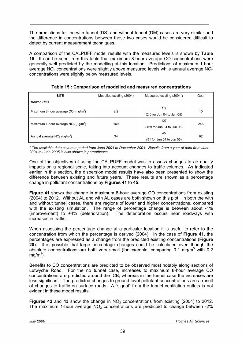
________________________________________________________________________
July 2006 _______________________________________________________________ Holmes Air Sciences
39
The predictions for the with tunnel (DS) and without tunnel (DM) cases are very similar and the difference in concentrations between these two cases would be considered difficult to detect by current measurement techniques.
A comparison of the CALPUFF model results with the measured levels is shown by Table15. It can be seen from this table that maximum 8-hour average CO concentrations were generally well predicted by the modelling at this location. Predictions of maximum 1-hour average NO2 concentrations were slightly above measured levels while annual average NO2concentrations were slightly below measured levels.
Table 15 : Comparison of modelled and measured concentrations
SITE Modelled existing (2004) Measured existing (2004*) Goal
Bowen Hills
Maximum 8-hour average CO (mg/m3) 2.2 1.9
(2.0 for Jun 04 to Jun 05) 10
Maximum 1-hour average NO2 (ug/m3) 169 127
(129 for Jun 04 to Jun 05) 246
Annual average NO2 (ug/m3) 34 45
(51 for Jun 04 to Jun 05) 62
* The available data covers a period from June 2004 to December 2004. Results from a year of data from June 2004 to June 2005 is also shown in parentheses.
One of the objectives of using the CALPUFF model was to assess changes to air quality impacts on a regional scale, taking into account changes to traffic volumes. As indicated earlier in this section, the dispersion model results have also been presented to show the difference between existing and future years. These results are shown as a percentage change in pollutant concentrations by Figures 41 to 45.
Figure 41 shows the change in maximum 8-hour average CO concentrations from existing (2004) to 2012. Without AL and with AL cases are both shown on this plot. In both the with and without tunnel cases, there are regions of lower and higher concentrations, compared with the existing simulation. The range of percentage change is between about -1% (improvement) to +4% (deterioration). The deterioration occurs near roadways with increases in traffic.
When assessing the percentage change at a particular location it is useful to refer to the concentration from which the percentage is derived (2004). In the case of Figure 41, the percentages are expressed as a change from the predicted existing concentrations (Figure20). It is possible that large percentage changes could be calculated even though the absolute concentrations are both very small (for example, comparing 0.1 mg/m3 with 0.2 mg/m3).
Benefits to CO concentrations are predicted to be observed most notably along sections of Lutwyche Road. For the no tunnel case, increases to maximum 8-hour average CO concentrations are predicted around the ICB, whereas in the tunnel case the increases are less significant. The predicted changes to ground-level pollutant concentrations are a result of changes to traffic on surface roads. A “signal” from the tunnel ventilation outlets is not evident in these model results.
Figures 42 and 43 show the change in NO2 concentrations from existing (2004) to 2012. The maximum 1-hour average NO2 concentrations are predicted to change between -2%
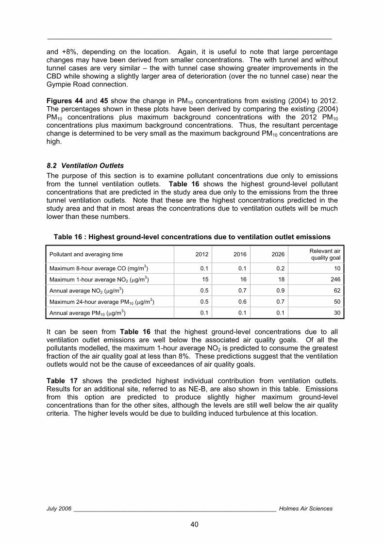
________________________________________________________________________
July 2006 _______________________________________________________________ Holmes Air Sciences
40
and +8%, depending on the location. Again, it is useful to note that large percentage changes may have been derived from smaller concentrations. The with tunnel and without tunnel cases are very similar – the with tunnel case showing greater improvements in the CBD while showing a slightly larger area of deterioration (over the no tunnel case) near the Gympie Road connection.
Figures 44 and 45 show the change in PM10 concentrations from existing (2004) to 2012. The percentages shown in these plots have been derived by comparing the existing (2004) PM10 concentrations plus maximum background concentrations with the 2012 PM10concentrations plus maximum background concentrations. Thus, the resultant percentage change is determined to be very small as the maximum background PM10 concentrations are high.
8.2 Ventilation Outlets The purpose of this section is to examine pollutant concentrations due only to emissions from the tunnel ventilation outlets. Table 16 shows the highest ground-level pollutant concentrations that are predicted in the study area due only to the emissions from the three tunnel ventilation outlets. Note that these are the highest concentrations predicted in the study area and that in most areas the concentrations due to ventilation outlets will be much lower than these numbers.
Table 16 : Highest ground-level concentrations due to ventilation outlet emissions
Pollutant and averaging time 2012 2016 2026 Relevant air quality goal
Maximum 8-hour average CO (mg/m3) 0.1 0.1 0.2 10
Maximum 1-hour average NO2 ( g/m3) 15 16 18 246
Annual average NO2 ( g/m3) 0.5 0.7 0.9 62
Maximum 24-hour average PM10 ( g/m3) 0.5 0.6 0.7 50
Annual average PM10 ( g/m3) 0.1 0.1 0.1 30
It can be seen from Table 16 that the highest ground-level concentrations due to all ventilation outlet emissions are well below the associated air quality goals. Of all the pollutants modelled, the maximum 1-hour average NO2 is predicted to consume the greatest fraction of the air quality goal at less than 8%. These predictions suggest that the ventilation outlets would not be the cause of exceedances of air quality goals.
Table 17 shows the predicted highest individual contribution from ventilation outlets. Results for an additional site, referred to as NE-B, are also shown in this table. Emissions from this option are predicted to produce slightly higher maximum ground-level concentrations than for the other sites, although the levels are still well below the air quality criteria. The higher levels would be due to building induced turbulence at this location.
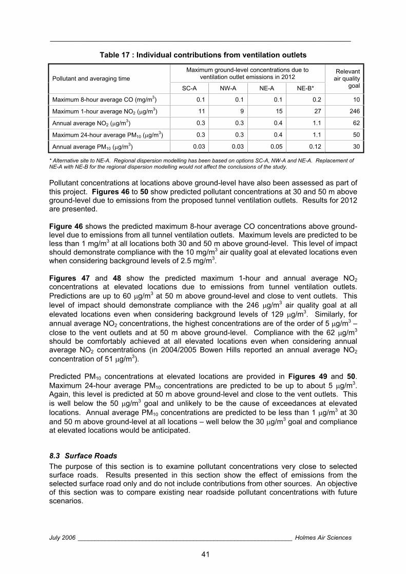
________________________________________________________________________
July 2006 _______________________________________________________________ Holmes Air Sciences
41
Table 17 : Individual contributions from ventilation outlets
Maximum ground-level concentrations due to ventilation outlet emissions in 2012 Pollutant and averaging time
SC-A NW-A NE-A NE-B*
Relevantair quality
goal
Maximum 8-hour average CO (mg/m3) 0.1 0.1 0.1 0.2 10
Maximum 1-hour average NO2 ( g/m3) 11 9 15 27 246
Annual average NO2 ( g/m3) 0.3 0.3 0.4 1.1 62
Maximum 24-hour average PM10 ( g/m3) 0.3 0.3 0.4 1.1 50
Annual average PM10 ( g/m3) 0.03 0.03 0.05 0.12 30
* Alternative site to NE-A. Regional dispersion modelling has been based on options SC-A, NW-A and NE-A. Replacement of NE-A with NE-B for the regional dispersion modelling would not affect the conclusions of the study.
Pollutant concentrations at locations above ground-level have also been assessed as part of this project. Figures 46 to 50 show predicted pollutant concentrations at 30 and 50 m above ground-level due to emissions from the proposed tunnel ventilation outlets. Results for 2012 are presented.
Figure 46 shows the predicted maximum 8-hour average CO concentrations above ground-level due to emissions from all tunnel ventilation outlets. Maximum levels are predicted to be less than 1 mg/m3 at all locations both 30 and 50 m above ground-level. This level of impact should demonstrate compliance with the 10 mg/m3 air quality goal at elevated locations even when considering background levels of 2.5 mg/m3.
Figures 47 and 48 show the predicted maximum 1-hour and annual average NO2concentrations at elevated locations due to emissions from tunnel ventilation outlets. Predictions are up to 60 g/m3 at 50 m above ground-level and close to vent outlets. This level of impact should demonstrate compliance with the 246 g/m3 air quality goal at all elevated locations even when considering background levels of 129 g/m3. Similarly, for annual average NO2 concentrations, the highest concentrations are of the order of 5 g/m3 – close to the vent outlets and at 50 m above ground-level. Compliance with the 62 g/m3
should be comfortably achieved at all elevated locations even when considering annual average NO2 concentrations (in 2004/2005 Bowen Hills reported an annual average NO2
concentration of 51 g/m3).
Predicted PM10 concentrations at elevated locations are provided in Figures 49 and 50.Maximum 24-hour average PM10 concentrations are predicted to be up to about 5 g/m3.Again, this level is predicted at 50 m above ground-level and close to the vent outlets. This is well below the 50 g/m3 goal and unlikely to be the cause of exceedances at elevated locations. Annual average PM10 concentrations are predicted to be less than 1 g/m3 at 30 and 50 m above ground-level at all locations – well below the 30 g/m3 goal and compliance at elevated locations would be anticipated.
8.3 Surface Roads The purpose of this section is to examine pollutant concentrations very close to selected surface roads. Results presented in this section show the effect of emissions from the selected surface road only and do not include contributions from other sources. An objective of this section was to compare existing near roadside pollutant concentrations with future scenarios.
________________________________________________________________________
July 2006 _______________________________________________________________ Holmes Air Sciences
42
Figures 51 to 61 present the results showing modelled near roadside pollutant concentrations. The predictions have been made using the Cal3qhcr roadway dispersion model. Each figure provides information for a single road section and presents the predictions of CO, NO2 and PM10 concentrations at various distances from the road for existing (2004) and future cases. Predictions have been made at the kerb and 10, 30 and 50 m from the eastern and western kerb of the road section. These predictions are useful for examining the differences between existing and future traffic scenarios.
Model predictions have taken into account a year of meteorological conditions (Bowen Hills data from July 2004 to June 2005).
From examination of the model results the highest pollutant concentrations for 2004 are predicted in the vicinity of the Gateway Motorway. This may be expected, given the very high traffic volumes experienced on this road. Predicted pollutant concentrations are highest at the kerb and decrease with distance from the kerb for all road sections. This shows the dispersion effect of distance from the source.
In assessing the magnitude of the predicted pollutant concentrations, an appropriate distance from the kerb should be selected based on the distance to the nearest residences. For example, the separation distance between the kerb and the nearest residences is greater for the Gateway Motorway than for many of the other selected roads. The most relevant distances from the Gateway Motorway section would be about 30 m while for most other sections, 10 m from the kerb would be the appropriate distance for the nearest residences.
The following observations were made from the surface road dispersion model predictions:
Predicted pollutant concentrations are highest at the kerb for each road section.
Predicted pollutant concentrations for 2004 are highest near the Gateway Motorway.
Road sections where the with tunnel case is predicted to be lower than the without tunnel case include Bowen Bridge Road, Sandgate Road, Newmarket Road and Lutwyche Road.
Road sections where the with tunnel case is predicted to be higher than the without tunnel case include Gympie Road, the Lutwyche Road/Gympie Road connection, Stafford Road and East-West Arterial Road.
Road sections where the differences between the with tunnel case and without tunnel cases are considered negligible include Gateway Motorway and Airport Drive.
Improvements in local air quality are observed with reductions in surface traffic that occur as a result of diverting traffic to the tunnel.
Concentrations near the Gateway Motorway are predicted to decrease significantly from 2004 to future scenarios. This is due to reduced traffic on this section as a result of the Gateway duplication project.
At distances appropriate for the nearest residences, the model predictions for all sections and future years are below the associated air quality goals.
________________________________________________________________________
July 2006 _______________________________________________________________ Holmes Air Sciences
43
Results for the AL Project with the proposed Northern Busway (NB) are also provided in Figures 51 to 61 (refer to “AL and NB” in the key). Examination of these results shows that near roadside concentrations for the AL with the busway would be very similar to concentrations without the busway. This is applicable to all modelled sections. Further discussion on the Project with the NB is provided in Section 9.1.
A useful comparison can also be made between predicted maximum pollutant concentrations due only to ventilation outlets (from Section 8.2) and maximum pollutant concentrations near surface roads. It is important not to underestimate the pollutant concentrations near surface roads as they are likely to be significantly higher than maximum levels expected as a result of emissions from tunnel ventilation outlets. Also, high pollutant concentrations near surface roads are likely to occur more often than high concentrations due to ventilation outlets.
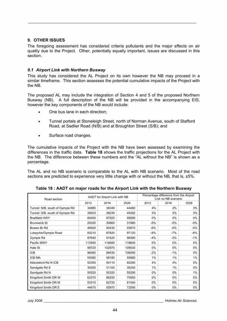
________________________________________________________________________
July 2006 _______________________________________________________________ Holmes Air Sciences
44
9. OTHER ISSUES The foregoing assessment has considered criteria pollutants and the major effects on air quality due to the Project. Other, potentially equally important, issues are discussed in this section.
9.1 Airport Link with Northern Busway This study has considered the AL Project on its own however the NB may proceed in a similar timeframe. This section assesses the potential cumulative impacts of the Project with the NB.
The proposed AL may include the integration of Section 4 and 5 of the proposed Northern Busway (NB). A full description of the NB will be provided in the accompanying EIS, however the key components of the NB would include:
One bus lane in each direction;
Tunnel portals at Stoneleigh Street, north of Norman Avenue, south of Stafford Road, at Sadlier Road (N/B) and at Broughton Street (S/B); and
Surface road changes.
The cumulative impacts of the Project with the NB have been assessed by examining the differences in the traffic data. Table 18 shows the traffic projections for the AL Project with the NB. The difference between these numbers and the “AL without the NB” is shown as a percentage.
The AL and no NB scenario is comparable to the AL with NB scenario. Most of the road sections are predicted to experience very little change with or without the NB, that is, ±5%.
Table 18 : AADT on major roads for the Airport Link with the Northern Busway
AADT for Airport Link with NB Percentage difference from the Airport Link no NB scenario Road section
2012 2016 2026 2012 2016 2026 Tunnel: N/B, south of Gympie Rd 34885 38349 44480 4% 2% 3% Tunnel: S/B, south of Gympie Rd 35623 38239 45282 3% 3% 3% Bradfield HWY 85400 87920 95690 0% 0% 0% Brunswick St 29320 30660 31960 -5% -5% -5% Bowen Br Rd 46920 50430 55870 -6% -5% -5% Lutwyche/Gympie Road 83210 87820 97120 -8% -7% -6% Gympie Rd 87640 91420 98380 -4% -3% -1% Pacific MWY 113940 116680 118600 0% 0% 0% Hale St 99720 102970 109030 0% 0% 0% ICB 96080 99430 106090 -2% -1% 0% ICB Nth 55080 58180 59980 1% 1% 1% Abbotsford Rd N ICB 52350 54110 60290 4% 4% 5% Sandgate Rd S 30300 31100 35250 1% 1% 0% Sandgate Rd N 50520 50320 55290 0% 0% 1% Kingsford Smith DR W 62370 66250 70950 0% 0% 0% Kingsford Smith DR M 53310 62720 81540 0% 0% 0% Kingsford Smith DR E 44670 50970 72090 0% 0% 0%
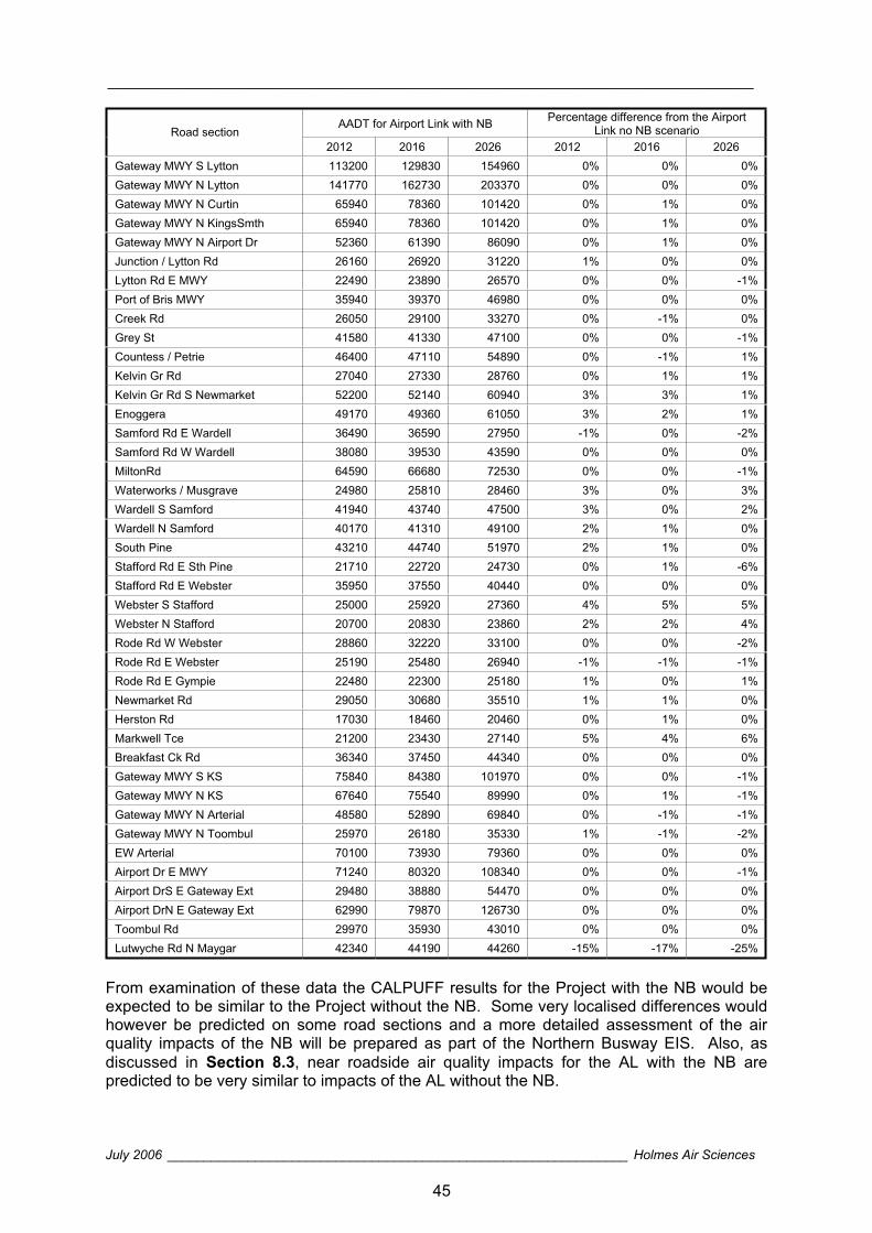
________________________________________________________________________
July 2006 _______________________________________________________________ Holmes Air Sciences
45
AADT for Airport Link with NB Percentage difference from the Airport Link no NB scenario Road section
2012 2016 2026 2012 2016 2026 Gateway MWY S Lytton 113200 129830 154960 0% 0% 0% Gateway MWY N Lytton 141770 162730 203370 0% 0% 0% Gateway MWY N Curtin 65940 78360 101420 0% 1% 0% Gateway MWY N KingsSmth 65940 78360 101420 0% 1% 0% Gateway MWY N Airport Dr 52360 61390 86090 0% 1% 0% Junction / Lytton Rd 26160 26920 31220 1% 0% 0% Lytton Rd E MWY 22490 23890 26570 0% 0% -1% Port of Bris MWY 35940 39370 46980 0% 0% 0% Creek Rd 26050 29100 33270 0% -1% 0% Grey St 41580 41330 47100 0% 0% -1% Countess / Petrie 46400 47110 54890 0% -1% 1% Kelvin Gr Rd 27040 27330 28760 0% 1% 1% Kelvin Gr Rd S Newmarket 52200 52140 60940 3% 3% 1% Enoggera 49170 49360 61050 3% 2% 1% Samford Rd E Wardell 36490 36590 27950 -1% 0% -2% Samford Rd W Wardell 38080 39530 43590 0% 0% 0% MiltonRd 64590 66680 72530 0% 0% -1% Waterworks / Musgrave 24980 25810 28460 3% 0% 3% Wardell S Samford 41940 43740 47500 3% 0% 2% Wardell N Samford 40170 41310 49100 2% 1% 0% South Pine 43210 44740 51970 2% 1% 0% Stafford Rd E Sth Pine 21710 22720 24730 0% 1% -6% Stafford Rd E Webster 35950 37550 40440 0% 0% 0% Webster S Stafford 25000 25920 27360 4% 5% 5% Webster N Stafford 20700 20830 23860 2% 2% 4% Rode Rd W Webster 28860 32220 33100 0% 0% -2% Rode Rd E Webster 25190 25480 26940 -1% -1% -1% Rode Rd E Gympie 22480 22300 25180 1% 0% 1% Newmarket Rd 29050 30680 35510 1% 1% 0% Herston Rd 17030 18460 20460 0% 1% 0% Markwell Tce 21200 23430 27140 5% 4% 6% Breakfast Ck Rd 36340 37450 44340 0% 0% 0% Gateway MWY S KS 75840 84380 101970 0% 0% -1% Gateway MWY N KS 67640 75540 89990 0% 1% -1% Gateway MWY N Arterial 48580 52890 69840 0% -1% -1% Gateway MWY N Toombul 25970 26180 35330 1% -1% -2% EW Arterial 70100 73930 79360 0% 0% 0% Airport Dr E MWY 71240 80320 108340 0% 0% -1% Airport DrS E Gateway Ext 29480 38880 54470 0% 0% 0% Airport DrN E Gateway Ext 62990 79870 126730 0% 0% 0% Toombul Rd 29970 35930 43010 0% 0% 0% Lutwyche Rd N Maygar 42340 44190 44260 -15% -17% -25%
From examination of these data the CALPUFF results for the Project with the NB would be expected to be similar to the Project without the NB. Some very localised differences would however be predicted on some road sections and a more detailed assessment of the air quality impacts of the NB will be prepared as part of the Northern Busway EIS. Also, as discussed in Section 8.3, near roadside air quality impacts for the AL with the NB are predicted to be very similar to impacts of the AL without the NB.
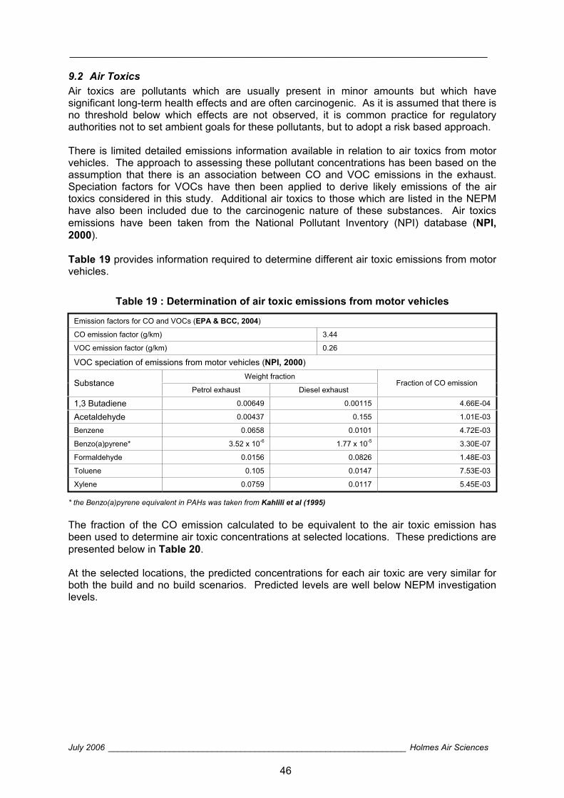
________________________________________________________________________
July 2006 _______________________________________________________________ Holmes Air Sciences
46
9.2 Air Toxics Air toxics are pollutants which are usually present in minor amounts but which have significant long-term health effects and are often carcinogenic. As it is assumed that there is no threshold below which effects are not observed, it is common practice for regulatory authorities not to set ambient goals for these pollutants, but to adopt a risk based approach.
There is limited detailed emissions information available in relation to air toxics from motor vehicles. The approach to assessing these pollutant concentrations has been based on the assumption that there is an association between CO and VOC emissions in the exhaust. Speciation factors for VOCs have then been applied to derive likely emissions of the air toxics considered in this study. Additional air toxics to those which are listed in the NEPM have also been included due to the carcinogenic nature of these substances. Air toxics emissions have been taken from the National Pollutant Inventory (NPI) database (NPI,2000).
Table 19 provides information required to determine different air toxic emissions from motor vehicles.
Table 19 : Determination of air toxic emissions from motor vehicles
Emission factors for CO and VOCs (EPA & BCC, 2004)
CO emission factor (g/km) 3.44
VOC emission factor (g/km) 0.26
VOC speciation of emissions from motor vehicles (NPI, 2000)Weight fraction
SubstancePetrol exhaust Diesel exhaust
Fraction of CO emission
1,3 Butadiene 0.00649 0.00115 4.66E-04
Acetaldehyde 0.00437 0.155 1.01E-03
Benzene 0.0658 0.0101 4.72E-03
Benzo(a)pyrene* 3.52 x 10⁻⁶ 1.77 x 10⁻⁵ 3.30E-07
Formaldehyde 0.0156 0.0826 1.48E-03
Toluene 0.105 0.0147 7.53E-03
Xylene 0.0759 0.0117 5.45E-03
* the Benzo(a)pyrene equivalent in PAHs was taken from Kahlili et al (1995)
The fraction of the CO emission calculated to be equivalent to the air toxic emission has been used to determine air toxic concentrations at selected locations. These predictions are presented below in Table 20.
At the selected locations, the predicted concentrations for each air toxic are very similar for both the build and no build scenarios. Predicted levels are well below NEPM investigation levels.
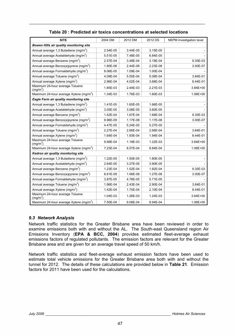
________________________________________________________________________
July 2006 _______________________________________________________________ Holmes Air Sciences
47
Table 20 : Predicted air toxics concentrations at selected locations
SITE 2004 DM 2012 DM 2012 DS NEPM investigation level Bowen Hills air quality monitoring siteAnnual average 1,3 Butadiene (mg/m3) 2.54E-05 3.44E-05 3.15E-05 - Annual average Acetaldehyde (mg/m3) 5.51E-05 7.48E-05 6.84E-05 - Annual average Benzene (mg/m3) 2.57E-04 3.48E-04 3.19E-04 9.35E-03 Annual average Benzo(a)pyrene (mg/m3) 1.80E-08 2.44E-08 2.23E-08 3.00E-07 Annual average Formaldehyde (mg/m3) 8.06E-05 1.09E-04 1.00E-04 - Annual average Toluene (mg/m3) 4.09E-04 5.55E-04 5.08E-04 3.84E-01 Annual average Xylene (mg/m3) 2.96E-04 4.02E-04 3.68E-04 8.44E-01 Maximum 24-hour average Toluene (mg/m3) 1.85E-03 2.44E-03 2.21E-03 3.84E+00
Maximum 24-hour average Xylene (mg/m3) 1.34E-03 1.76E-03 1.60E-03 1.06E+00 Eagle Farm air quality monitoring siteAnnual average 1,3 Butadiene (mg/m3) 1.41E-05 1.65E-05 1.66E-05 - Annual average Acetaldehyde (mg/m3) 3.05E-05 3.58E-05 3.60E-05 - Annual average Benzene (mg/m3) 1.42E-04 1.67E-04 1.68E-04 9.35E-03 Annual average Benzo(a)pyrene (mg/m3) 9.96E-09 1.17E-08 1.17E-08 3.00E-07 Annual average Formaldehyde (mg/m3) 4.47E-05 5.24E-05 5.27E-05 - Annual average Toluene (mg/m3) 2.27E-04 2.66E-04 2.68E-04 3.84E-01 Annual average Xylene (mg/m3) 1.64E-04 1.93E-04 1.94E-04 8.44E-01 Maximum 24-hour average Toluene (mg/m3) 9.99E-04 1.18E-03 1.22E-03 3.84E+00
Maximum 24-hour average Xylene (mg/m3) 7.23E-04 8.57E-04 8.84E-04 1.06E+00 Kedron air quality monitoring siteAnnual average 1,3 Butadiene (mg/m3) 1.22E-05 1.50E-05 1.80E-05 - Annual average Acetaldehyde (mg/m3) 2.64E-05 3.27E-05 3.90E-05 - Annual average Benzene (mg/m3) 1.23E-04 1.52E-04 1.82E-04 9.35E-03 Annual average Benzo(a)pyrene (mg/m3) 8.61E-09 1.06E-08 1.27E-08 3.00E-07 Annual average Formaldehyde (mg/m3) 3.87E-05 4.78E-05 5.71E-05 - Annual average Toluene (mg/m3) 1.96E-04 2.43E-04 2.90E-04 3.84E-01 Annual average Xylene (mg/m3) 1.42E-04 1.75E-04 2.10E-04 8.44E-01 Maximum 24-hour average Toluene (mg/m3) 1.04E-03 1.26E-03 1.24E-03 3.84E+00
Maximum 24-hour average Xylene (mg/m3) 7.50E-04 9.08E-04 8.94E-04 1.06E+00
9.3 Network Analysis Network traffic statistics for the Greater Brisbane area have been reviewed in order to examine emissions both with and without the AL. The South-east Queensland region Air Emissions Inventory (EPA & BCC, 2004) provides estimated fleet-average exhaust emissions factors of regulated pollutants. The emission factors are relevant for the Greater Brisbane area and are given for an average travel speed of 50 km/h.
Network traffic statistics and fleet-average exhaust emission factors have been used to estimate total vehicle emissions for the Greater Brisbane area both with and without the tunnel for 2012. The details of these calculations are provided below in Table 21. Emission factors for 2011 have been used for the calculations.
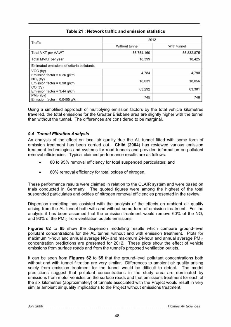
________________________________________________________________________
July 2006 _______________________________________________________________ Holmes Air Sciences
48
Table 21 : Network traffic and emission statistics
2012Traffic
Without tunnel With tunnel
Total VKT per AAWT 55,754,160 55,832,875
Total MVKT per year 18,399 18,425
Estimated emissions of criteria pollutants VOC (t/y) Emission factor = 0.26 g/km 4,784 4,790
NOx (t/y) Emission factor = 0.98 g/km 18,031 18,056
CO (t/y) Emission factor = 3.44 g/km 63,292 63,381
PM10 (t/y) Emission factor = 0.0405 g/km 745 746
Using a simplified approach of multiplying emission factors by the total vehicle kilometres travelled, the total emissions for the Greater Brisbane area are slightly higher with the tunnel than without the tunnel. The differences are considered to be marginal.
9.4 Tunnel Filtration Analysis An analysis of the effect on local air quality due the AL tunnel fitted with some form of emission treatment has been carried out. Child (2004) has reviewed various emission treatment technologies and systems for road tunnels and provided information on pollutant removal efficiencies. Typical claimed performance results are as follows:
80 to 95% removal efficiency for total suspended particulates; and
60% removal efficiency for total oxides of nitrogen.
These performance results were claimed in relation to the CLAIR system and were based on trials conducted in Germany. The quoted figures were among the highest of the total suspended particulates and oxides of nitrogen removal efficiencies presented in the review.
Dispersion modelling has assisted with the analysis of the effects on ambient air quality arising from the AL tunnel both with and without some form of emission treatment. For the analysis it has been assumed that the emission treatment would remove 60% of the NOxand 90% of the PM10 from ventilation outlets emissions.
Figures 62 to 65 show the dispersion modelling results which compare ground-level pollutant concentrations for the AL tunnel without and with emission treatment. Plots for maximum 1-hour and annual average NO2 and maximum 24-hour and annual average PM10concentration predictions are presented for 2012. These plots show the effect of vehicle emissions from surface roads and from the tunnel’s proposed ventilation outlets.
It can be seen from Figures 62 to 65 that the ground-level pollutant concentrations both without and with tunnel filtration are very similar. Differences to ambient air quality arising solely from emission treatment for the tunnel would be difficult to detect. The model predictions suggest that pollutant concentrations in the study area are dominated by emissions from motor vehicles on the surface roads and that emissions treatment for each of the six kilometres (approximately) of tunnels associated with the Project would result in very similar ambient air quality implications to the Project without emissions treatment.
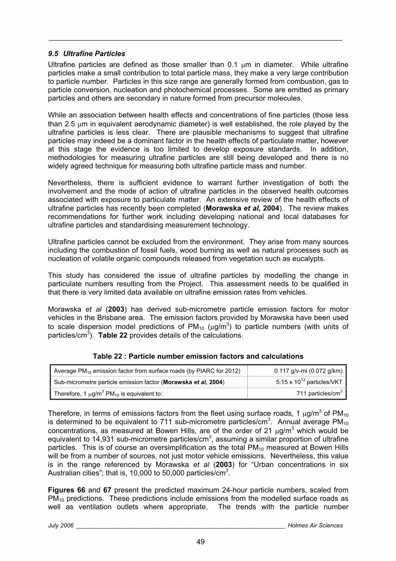
________________________________________________________________________
July 2006 _______________________________________________________________ Holmes Air Sciences
49
9.5 Ultrafine Particles Ultrafine particles are defined as those smaller than 0.1 m in diameter. While ultrafine particles make a small contribution to total particle mass, they make a very large contribution to particle number. Particles in this size range are generally formed from combustion, gas to particle conversion, nucleation and photochemical processes. Some are emitted as primary particles and others are secondary in nature formed from precursor molecules.
While an association between health effects and concentrations of fine particles (those less than 2.5 m in equivalent aerodynamic diameter) is well established, the role played by the ultrafine particles is less clear. There are plausible mechanisms to suggest that ultrafine particles may indeed be a dominant factor in the health effects of particulate matter, however at this stage the evidence is too limited to develop exposure standards. In addition, methodologies for measuring ultrafine particles are still being developed and there is no widely agreed technique for measuring both ultrafine particle mass and number.
Nevertheless, there is sufficient evidence to warrant further investigation of both the involvement and the mode of action of ultrafine particles in the observed health outcomes associated with exposure to particulate matter. An extensive review of the health effects of ultrafine particles has recently been completed (Morawska et al, 2004). The review makes recommendations for further work including developing national and local databases for ultrafine particles and standardising measurement technology.
Ultrafine particles cannot be excluded from the environment. They arise from many sources including the combustion of fossil fuels, wood burning as well as natural processes such as nucleation of volatile organic compounds released from vegetation such as eucalypts.
This study has considered the issue of ultrafine particles by modelling the change in particulate numbers resulting from the Project. This assessment needs to be qualified in that there is very limited data available on ultrafine emission rates from vehicles.
Morawska et al (2003) has derived sub-micrometre particle emission factors for motor vehicles in the Brisbane area. The emission factors provided by Morawska have been used to scale dispersion model predictions of PM10 ( g/m3) to particle numbers (with units of particles/cm3). Table 22 provides details of the calculations.
Table 22 : Particle number emission factors and calculations
Average PM10 emission factor from surface roads (by PIARC for 2012) 0.117 g/v-mi (0.072 g/km)
Sub-micrometre particle emission factor (Morawska et al, 2004) 5.15 x 10¹³ particles/VKT
Therefore, 1 g/m3 PM10 is equivalent to: 711 particles/cm3
Therefore, in terms of emissions factors from the fleet using surface roads, 1 g/m3 of PM10is determined to be equivalent to 711 sub-micrometre particles/cm3. Annual average PM10
concentrations, as measured at Bowen Hills, are of the order of 21 g/m3 which would be equivalent to 14,931 sub-micrometre particles/cm3, assuming a similar proportion of ultrafine particles. This is of course an oversimplification as the total PM10 measured at Bowen Hills will be from a number of sources, not just motor vehicle emissions. Nevertheless, this value is in the range referenced by Morawska et al (2003) for “Urban concentrations in six Australian cities”; that is, 10,000 to 50,000 particles/cm3.
Figures 66 and 67 present the predicted maximum 24-hour particle numbers, scaled from PM10 predictions. These predictions include emissions from the modelled surface roads as well as ventilation outlets where appropriate. The trends with the particle number

________________________________________________________________________
July 2006 _______________________________________________________________ Holmes Air Sciences
50
predictions (that is, comparisons between scenarios) are the same as those observed for the PM10 predictions suggesting very little difference between the build and no build scenarios.
________________________________________________________________________
July 2006 _______________________________________________________________ Holmes Air Sciences
51
10. CONCLUSIONS This report has assessed the effects on air quality of the proposed Airport Link Tunnel in Brisbane. Dispersion modelling has been used as the primary tool to quantitatively assess pollutant concentrations in the study area.
The conclusions of the study can be summarised as follows:
Pollutant concentrations in the study area in future years (2012+) arising from motor vehicles would be expected to be similar to existing (2004) concentrations.This is the case both with and without the Project.
Model results for future years are considered to be conservative since no further improvements to vehicle emissions have been taken into account.
Particulate matter concentrations arising from non-motor vehicle sources, such as bushfires, may continue to result in elevated levels on occasions.
At ground-level the with and without tunnel cases are predicted to be very similar. That is, regional air quality with the Project may be expected to be similar to air quality without the Project.
At ground-level the highest concentrations due to emissions from ventilation outlets are predicted to be much less than concentrations near busy surface roads.
Pollutant concentrations at elevated locations due to ventilation outlet emissions would be expected to be below relevant air quality goals.
An analysis of network traffic flow suggests that total emissions in the Greater Brisbane area would be slightly higher with the Project than without. The differences in emissions are considered to be marginal.
The difference in ambient air quality arising from treatment of tunnel emissions by some form of filtration would be difficult to detect. Benefits arising from emissions treatment would most likely be realised in-tunnel and at elevated locations very near the tunnel ventilation outlets.
Air quality impacts arising from the Project with the proposed Northern Busway would be expected to be very similar to the Project without the Northern Busway.
It is concluded from the study that there would be no adverse air quality impacts as a direct result of the Project. The reader should refer to each section of the report for more detailed examination of specific air quality issues associated with the Project.
________________________________________________________________________
July 2006 _______________________________________________________________ Holmes Air Sciences
52
11. REFERENCES ABS (2003)
Australian Bureau of Statistics: Motor Vehicle Census, Document 9309.0, 31 March 2003
Bureau of Meteorology (2006) Climate averages from the Bureau of Meteorology website, www.bom.gov.au
Carnovale F, and Tilly K (1995) "MAQS Consultancy - Emissions Inventory Report" prepared by the Environment Protection Authority of Victoria, 1995.
Child and Associates (2004) “M5 East Freeway: A review of emission treatment technologies, systems and applications”, by Child N and Associates for the Roads and Traffic Authority of NSW, September 2004.
DEC (2005) “Approved Methods for the Modelling and Assessment of Air Pollutants in NSW”, August 2005.
Environment Australia (2003) “Technical Report No. 1: Toxic Emissions from Diesel Vehicles in Australia”. May 2003.
EPA (1994) “Environmental Protection Act 1994”, prepared the Office of the Queensland Parliamentary Counsel, reprint No. 5C.
EPA (1997) “Environmental Protection (Air) Policy 1997, prepared the Office of the Queensland Parliamentary Counsel, reprint No. 2A.
EPA & BCC (2004) “Air Emissions Inventory: South-east Queensland region”. Prepared by a partnership between Brisbane City Council and the Queensland Government Environmental Protection Agency, 2004.
Health Effects Institute (2003) “Revised analyses of time-series studies of air pollution and health” Special Report May 2003
Holmes Air Sciences (1997) “RTA air quality monitoring program”, prepared for the NSW Roads and Traffic Authority, January 1997
Holmes Air Sciences (2001) “Air Quality Assessment: Lane Cove Tunnel”, prepared by Holmes Air Sciences for Sinclair Knight Merz on behalf of the Roads and Traffic Authority, October 2001.
________________________________________________________________________
July 2006 _______________________________________________________________ Holmes Air Sciences
53
Holmes Air Sciences (2004) “Air Quality Impact Assessment: Brisbane North-South Bypass Tunnel”, prepared by Holmes Air Sciences for Sinclair Knight Merz / Connell Wagner Joint Venture on behalf of Brisbane City Council, December 2004.
Hurley, P J (2002) "The Air Pollution Model (TAPM) Version 2 : User Manual", CSIRO Atmospheric Research Internal Paper No. 25, April 2002
Kahlili N R, Scheff A P, and Holsen T M (1995) “PAH source fingerprints for coke ovens, diesel and gasoline engines, highway tunnels and wood combustion emissions”, Atmos. Environ 29, pp 533-542.
Morawska L, Moore MR, Ristovksi ZD (2004) “Health Impacts of Ultrafine Particles” prepared for Australian Government, Department of Environment and Heritage, 2004.
Morawska L, Thomas S, Jamriska M, Ferreira L, McGregor F (2003) “Quantification of motor vehicle emission factors from on road measurements”.
NEPC (1998) “National Environment Protection Measure”, prepared by the National Environment Protection Council, June 1998 2004.”
NEPC (2004) “National Environment Protection (Air Toxics) Measure”, prepared by the National Environment Protection Council, April 2004.
NPI (2000) “National Pollutant Inventory: Emissions estimation technique manual for aggregated emissions from motor vehicles”, 22 November 2000 Version 1.0
NSW EPA, CSIRO, RTA (1996) “Sydney Harbour Tunnel – Air Quality Study” Draft Report No. 1.
Pacific Power (1998) “Illawarra Ecoenergy Park: Combined Cycle Gas Turbine Power Station”, Environmental Impact Statement
PIARC (1995) “Vehicle Emissions, Air Demand, Environment, Longitudinal Ventilation”, Committee on Road Tunnels, XXth World Road Congress, Montreal, ISBN 2-84060-034-X
PIARC (2004) “Road Tunnels: Vehicle Emissions and Air Demand for Ventilation”, PIARC Technical Committee on Road Tunnels, ISBN 2-84060-177-X, November 2004.
PPK (1999) “Second Sydney Airport”, Supplement to Draft Environmental Impact Statement
Puri, K., Dietachmayer, G. S., Mills, G. A., Davidson, N. E., Bowen, R. A., and Logan, L. W (1997)
“The BMRC Limited Area Prediction System, LAPS”. Aust. Met. Mag., 47, 203-223
RTA (2000)
________________________________________________________________________
July 2006 _______________________________________________________________ Holmes Air Sciences
54
“Cross City Tunnel”, Environmental Impact Statement prepared by PPK Environment and Infrastructure, June 2000
________________________________________________________________________
July 2006 _______________________________________________________________ Holmes Air Sciences
APPENDIX A HEALTH EFFECTS OF POLLUTANTS EMITTED FROM MOTOR
VEHICLES
________________________________________________________________________
July 2006 _______________________________________________________________ Holmes Air Sciences
APPENDIX A HEALTH EFFECTS OF POLLUTANTS EMITTED FROM MOTOR VEHICLES
The following sections discuss the health effects of the various pollutants and compounds referred to in the report.
Carbon monoxide Carbon monoxide can be harmful to humans because its affinity for haemoglobin is more than 200 times greater than that of oxygen. When it is inhaled it is taken up by the blood and therefore reduces the capacity of the blood to transport oxygen. This process is reversible and reducing the exposure will lead to the establishment of a new equilibrium with a period of three hours being the approximate time required to reach 50% of the equilibrium value.
Symptoms of carbon monoxide intoxication are lassitude and headaches; however these are generally not reported until the concentrations of carboxyhaemoglobin in the blood are in excess of 10% of saturation. This is approximately the equilibrium value achieved with an ambient atmospheric concentration of 70 mg/m3 for a person engaged in light activity. However, there is evidence that there is a risk for individuals with cardiovascular disease when the carboxyhaemoglobin concentration reaches 4% and the WHO recommends that ambient concentrations be kept to values which would protect individuals from exceeding the 4% level.
The 8-hour goals noted by the EPA and NEPM provide a significant margin for safety, however this is appropriate for this type of guideline, which is designed to protect a wide range of people in the community including the very young and elderly.
Oxides of nitrogen Nitrogen oxides (NOx) emitted from combustion sources are comprised mainly of nitric oxide (NO, approximately 95% at the point of emission) and nitrogen dioxide (NO2, approximately 5% at the point of emission). Nitric oxide is much less harmful to humans than nitrogen dioxide and is not generally considered a pollutant with health impacts at the concentrations normally found in urban environments. Concern with nitric oxide relates to its transformation to nitrogen dioxide and its role in the formation of photochemical smog. Nitrogen dioxide has been reported to have an effect on respiratory function although the evidence concerning effects has been mixed and conflicting. The EPA has not set any air quality goals for nitric oxide, however it has set 1-hour and annual average goals for nitrogen dioxide.
Particulate matter The presence of particulate matter in the atmosphere can have an adverse effect on health and amenity. The health effects of particles are largely related to the extent to which they can penetrate the respiratory tract. Larger particles, that is those greater than 10 m,generally adhere to the mucous in the nose, mouth, pharynx and larger bronchi and from there are removed by either swallowing or expectorating. Finer particles can enter bronchial and pulmonary regions of the respiratory tract, with increased deposition during mouth breathing which increases during exercise. The very fine particles can be deposited in the pulmonary region and it is these which are of particular concern.
The health effects of particulate matter are further complicated by the chemical nature of the particles and by the possibility of synergistic effects with other air pollutants such as sulfur dioxide.
________________________________________________________________________
July 2006 _______________________________________________________________ Holmes Air Sciences
Much of the recent concern over the health effects of fine particulate matter is based on investigations carried out in the US, with the view to quantifying the health risks associated with both long-term and short-term exposure to airborne particulate matter. The study is colloquially referred to as "The Six Cities Study" from the original work by Dockery et al. (1993), which determined a relationship between fine particulate matter (defined as particles smaller than 2.5 m in diameter) in the air and mortality in six US cities.
The basic findings of the Six Cities Study is that there is an increase in mortality with increasing concentrations of fine particulate matter. The conclusions appear to be robust and have been supported by subsequent studies and as far as can be determined are not confounded by other known variables. It is important to note that the observed association between fine particles and mortality is statistical. The particles are not the primary cause of death, but are one of many environmental and other risk factors. More recently the statistical associations have been revised downwards based on a review of the statistical methods used, but the association remains (HEI, 2003). However the current Australian air quality goals for particulate matter are still based on the more conservative associations.
HydrocarbonsHydrocarbons alone do not generally pose a problem at the concentrations commonly experienced. However, some hydrocarbons such as benzene are known to have an adverse effect on human health (see later), but the effects are thought to occur at concentrations higher than the levels of exposure found at roadsides from traffic emissions. Hydrocarbons do play a significant role in photochemical smog formation and until recently the air quality standards adopted by the US EPA for non-methane hydrocarbons have been applied in NSW. However it has been recognised that this goal does not distinguish the reactive species which are involved in smog formation from the total hydrocarbon concentration and this air quality goal has been abandoned by the US EPA.
There is growing concern about the amount of benzene released in motor vehicle emissions, especially in Europe where fuel has a higher benzene and aromatic content than in Australia. At present Queensland has no ambient air quality goals for benzene. The Victorian EPA currently has a limit of 0.10 mg/m3 (0.033 ppm) (3-minute average). Many in the scientific community hold the view that there is no safe limit for benzene. The WHO specifies a risk factor for developing leukaemia of 4x10⁻⁶ for a lifetime exposure to 1 g/m3.The United Kingdom has an annual average ambient benzene goal of 5 parts per billion (ppb) or 16 g/m3 to be achieved by 2005. The 5 ppb goal is based on the "No Observable Adverse Effect Level" from the findings of the UK Expert Panel on Air Quality Standards that the risk of leukaemia in workers would not be detectable when the average working lifetime exposure to benzene was less than 500 ppb. Two safety factors of 10 were then applied to derive the goal of 5 ppb. The NEPM (Air Toxics) air quality goal for benzene is 3 ppb.

________________________________________________________________________
July 2006 _______________________________________________________________ Holmes Air Sciences
APPENDIX B JOINT WIND SPEED, WIND DIRECTION AND STABILITY CLASS
FREQUENCY TABLES

________________________________________________________________________
July 2006 _______________________________________________________________ Holmes Air Sciences
APPENDIX B JOINT WIND SPEED, WIND DIRECTION AND STABILITY CLASS FREQUENCY TABLES
This section provides meteorological information including
A list of missing BoM upper-air data records;
Joint wind speed, wind direction and stability class frequency tables for Brisbane Airport;
Missing upper-air data records Upper air data collected by the Bureau of Meteorology at Brisbane Airport in 2004 were not a complete dataset for the purposes of the CALMET modelling. The missing periods are listed below.
Gap between soundings is greater than 14 hours before: 13 Jan 2004 hour 11 GMT Gap between soundings is greater than 14 hours before: 10 Feb 2004 Hour 11 GMT Gap between soundings is greater than 14 hours before: 23 Feb 2004 Hour 23 GMT
The missing soundings were supplemented with output from the TAPM model.
Joint wind speed, wind direction and stability class frequency tables
STATISTICS FOR FILE: C:\Jobs\BACNPR\calmet\prtmet\bap2004.aus (Brisbane Airport by CALMET) MONTHS: All HOURS : All OPTION: Frequency
PASQUILL STABILITY CLASS 'A'
Wind Speed Class (m/s)
0.50 1.50 3.00 4.50 6.00 7.50 9.00 GREATER WIND TO TO TO TO TO TO TO THAN SECTOR 1.50 3.00 4.50 6.00 7.50 9.00 10.50 10.50 TOTAL -----------------------------------------------------------------------------------------
NNE 0.000000 0.000000 0.000000 0.000000 0.000000 0.000000 0.000000 0.000000 0.000000 NE 0.000000 0.000000 0.000000 0.000000 0.000000 0.000000 0.000000 0.000000 0.000000 ENE 0.000000 0.000000 0.000000 0.000000 0.000000 0.000000 0.000000 0.000000 0.000000 E 0.000000 0.000000 0.000000 0.000000 0.000000 0.000000 0.000000 0.000000 0.000000 ESE 0.000000 0.000000 0.000000 0.000000 0.000000 0.000000 0.000000 0.000000 0.000000 SE 0.000000 0.000000 0.000000 0.000000 0.000000 0.000000 0.000000 0.000000 0.000000 SSE 0.000000 0.000000 0.000000 0.000000 0.000000 0.000000 0.000000 0.000000 0.000000 S 0.000114 0.000000 0.000000 0.000000 0.000000 0.000000 0.000000 0.000000 0.000114 SSW 0.000000 0.000000 0.000000 0.000000 0.000000 0.000000 0.000000 0.000000 0.000000 SW 0.000000 0.000000 0.000000 0.000000 0.000000 0.000000 0.000000 0.000000 0.000000 WSW 0.000000 0.000000 0.000000 0.000000 0.000000 0.000000 0.000000 0.000000 0.000000 W 0.000000 0.000000 0.000000 0.000000 0.000000 0.000000 0.000000 0.000000 0.000000 WNW 0.000000 0.000000 0.000000 0.000000 0.000000 0.000000 0.000000 0.000000 0.000000 NW 0.000000 0.000114 0.000000 0.000000 0.000000 0.000000 0.000000 0.000000 0.000114 NNW 0.000000 0.000000 0.000000 0.000000 0.000000 0.000000 0.000000 0.000000 0.000000 N 0.000000 0.000000 0.000000 0.000000 0.000000 0.000000 0.000000 0.000000 0.000000
CALM 0.000000 ----------------------------------------------------------------------------------------- TOTAL 0.000114 0.000114 0.000000 0.000000 0.000000 0.000000 0.000000 0.000000 0.000228
MEAN WIND SPEED (m/s) = 1.70 NUMBER OF OBSERVATIONS = 2
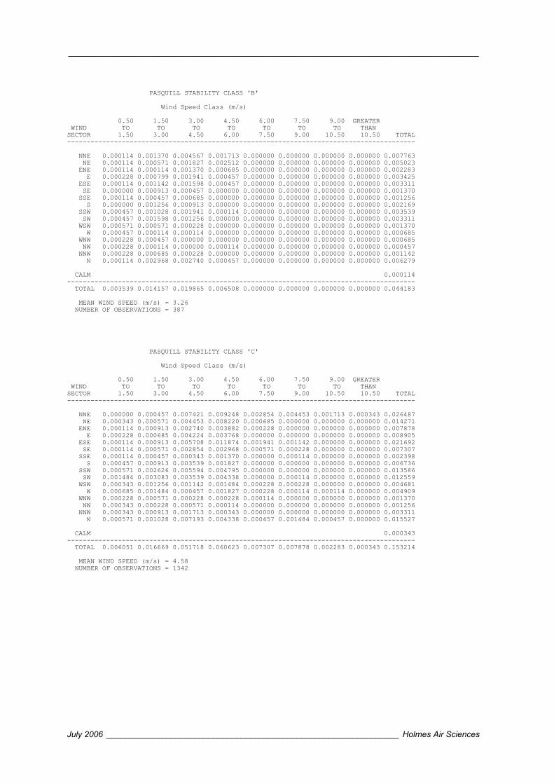
________________________________________________________________________
July 2006 _______________________________________________________________ Holmes Air Sciences
PASQUILL STABILITY CLASS 'B'
Wind Speed Class (m/s)
0.50 1.50 3.00 4.50 6.00 7.50 9.00 GREATER WIND TO TO TO TO TO TO TO THAN SECTOR 1.50 3.00 4.50 6.00 7.50 9.00 10.50 10.50 TOTAL -----------------------------------------------------------------------------------------
NNE 0.000114 0.001370 0.004567 0.001713 0.000000 0.000000 0.000000 0.000000 0.007763 NE 0.000114 0.000571 0.001827 0.002512 0.000000 0.000000 0.000000 0.000000 0.005023 ENE 0.000114 0.000114 0.001370 0.000685 0.000000 0.000000 0.000000 0.000000 0.002283 E 0.000228 0.000799 0.001941 0.000457 0.000000 0.000000 0.000000 0.000000 0.003425 ESE 0.000114 0.001142 0.001598 0.000457 0.000000 0.000000 0.000000 0.000000 0.003311 SE 0.000000 0.000913 0.000457 0.000000 0.000000 0.000000 0.000000 0.000000 0.001370 SSE 0.000114 0.000457 0.000685 0.000000 0.000000 0.000000 0.000000 0.000000 0.001256 S 0.000000 0.001256 0.000913 0.000000 0.000000 0.000000 0.000000 0.000000 0.002169 SSW 0.000457 0.001028 0.001941 0.000114 0.000000 0.000000 0.000000 0.000000 0.003539 SW 0.000457 0.001598 0.001256 0.000000 0.000000 0.000000 0.000000 0.000000 0.003311 WSW 0.000571 0.000571 0.000228 0.000000 0.000000 0.000000 0.000000 0.000000 0.001370 W 0.000457 0.000114 0.000114 0.000000 0.000000 0.000000 0.000000 0.000000 0.000685 WNW 0.000228 0.000457 0.000000 0.000000 0.000000 0.000000 0.000000 0.000000 0.000685 NW 0.000228 0.000114 0.000000 0.000114 0.000000 0.000000 0.000000 0.000000 0.000457 NNW 0.000228 0.000685 0.000228 0.000000 0.000000 0.000000 0.000000 0.000000 0.001142 N 0.000114 0.002968 0.002740 0.000457 0.000000 0.000000 0.000000 0.000000 0.006279
CALM 0.000114 ----------------------------------------------------------------------------------------- TOTAL 0.003539 0.014157 0.019865 0.006508 0.000000 0.000000 0.000000 0.000000 0.044183
MEAN WIND SPEED (m/s) = 3.26 NUMBER OF OBSERVATIONS = 387
PASQUILL STABILITY CLASS 'C'
Wind Speed Class (m/s)
0.50 1.50 3.00 4.50 6.00 7.50 9.00 GREATER WIND TO TO TO TO TO TO TO THAN SECTOR 1.50 3.00 4.50 6.00 7.50 9.00 10.50 10.50 TOTAL -----------------------------------------------------------------------------------------
NNE 0.000000 0.000457 0.007421 0.009248 0.002854 0.004453 0.001713 0.000343 0.026487 NE 0.000343 0.000571 0.004453 0.008220 0.000685 0.000000 0.000000 0.000000 0.014271 ENE 0.000114 0.000913 0.002740 0.003882 0.000228 0.000000 0.000000 0.000000 0.007878 E 0.000228 0.000685 0.004224 0.003768 0.000000 0.000000 0.000000 0.000000 0.008905 ESE 0.000114 0.000913 0.005708 0.011874 0.001941 0.001142 0.000000 0.000000 0.021692 SE 0.000114 0.000571 0.002854 0.002968 0.000571 0.000228 0.000000 0.000000 0.007307 SSE 0.000114 0.000457 0.000343 0.001370 0.000000 0.000114 0.000000 0.000000 0.002398 S 0.000457 0.000913 0.003539 0.001827 0.000000 0.000000 0.000000 0.000000 0.006736 SSW 0.000571 0.002626 0.005594 0.004795 0.000000 0.000000 0.000000 0.000000 0.013586 SW 0.001484 0.003083 0.003539 0.004338 0.000000 0.000114 0.000000 0.000000 0.012559 WSW 0.000343 0.001256 0.001142 0.001484 0.000228 0.000228 0.000000 0.000000 0.004681 W 0.000685 0.001484 0.000457 0.001827 0.000228 0.000114 0.000114 0.000000 0.004909 WNW 0.000228 0.000571 0.000228 0.000228 0.000114 0.000000 0.000000 0.000000 0.001370 NW 0.000343 0.000228 0.000571 0.000114 0.000000 0.000000 0.000000 0.000000 0.001256 NNW 0.000343 0.000913 0.001713 0.000343 0.000000 0.000000 0.000000 0.000000 0.003311 N 0.000571 0.001028 0.007193 0.004338 0.000457 0.001484 0.000457 0.000000 0.015527
CALM 0.000343 ----------------------------------------------------------------------------------------- TOTAL 0.006051 0.016669 0.051718 0.060623 0.007307 0.007878 0.002283 0.000343 0.153214
MEAN WIND SPEED (m/s) = 4.58 NUMBER OF OBSERVATIONS = 1342
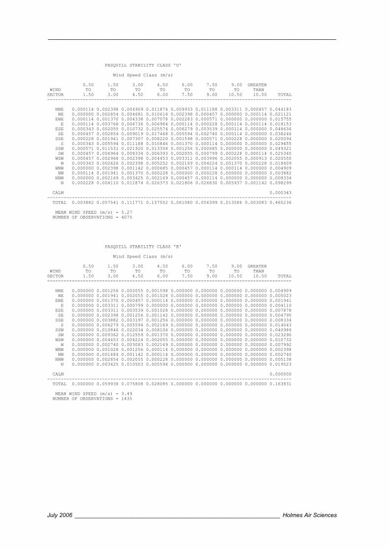
________________________________________________________________________
July 2006 _______________________________________________________________ Holmes Air Sciences
PASQUILL STABILITY CLASS 'D'
Wind Speed Class (m/s)
0.50 1.50 3.00 4.50 6.00 7.50 9.00 GREATER WIND TO TO TO TO TO TO TO THAN SECTOR 1.50 3.00 4.50 6.00 7.50 9.00 10.50 10.50 TOTAL -----------------------------------------------------------------------------------------
NNE 0.000114 0.002398 0.004909 0.011874 0.009933 0.011188 0.003311 0.000457 0.044183 NE 0.000000 0.002854 0.004681 0.010618 0.002398 0.000457 0.000000 0.000114 0.021121 ENE 0.000114 0.001370 0.004338 0.007078 0.002283 0.000571 0.000000 0.000000 0.015755 E 0.000114 0.003768 0.006736 0.006964 0.000114 0.000228 0.000114 0.000114 0.018153 ESE 0.000343 0.002055 0.010732 0.025574 0.006279 0.003539 0.000114 0.000000 0.048636 SE 0.000457 0.002854 0.009019 0.017468 0.005594 0.002740 0.000114 0.000000 0.038246 SSE 0.000228 0.001941 0.007307 0.008220 0.001598 0.000571 0.000228 0.000000 0.020094 S 0.000343 0.005594 0.011188 0.010846 0.001370 0.000114 0.000000 0.000000 0.029455 SSW 0.000571 0.011531 0.021920 0.013358 0.001256 0.000685 0.000000 0.000000 0.049321 SW 0.000457 0.006964 0.008334 0.006393 0.002055 0.000799 0.000228 0.000114 0.025345 WSW 0.000457 0.002968 0.002398 0.004453 0.003311 0.003996 0.002055 0.000913 0.020550 W 0.000343 0.002626 0.002398 0.005252 0.002169 0.004224 0.001370 0.000228 0.018609 WNW 0.000000 0.002398 0.001142 0.000685 0.000457 0.000114 0.000114 0.000000 0.004909 NW 0.000114 0.001941 0.001370 0.000228 0.000000 0.000228 0.000000 0.000000 0.003882 NNW 0.000000 0.002169 0.003425 0.002169 0.000457 0.000114 0.000000 0.000000 0.008334 N 0.000228 0.004110 0.011874 0.026373 0.021806 0.026830 0.005937 0.001142 0.098299
CALM 0.000343 ----------------------------------------------------------------------------------------- TOTAL 0.003882 0.057541 0.111771 0.157552 0.061080 0.056399 0.013586 0.003083 0.465236
MEAN WIND SPEED (m/s) = 5.27 NUMBER OF OBSERVATIONS = 4075
PASQUILL STABILITY CLASS 'E'
Wind Speed Class (m/s)
0.50 1.50 3.00 4.50 6.00 7.50 9.00 GREATER WIND TO TO TO TO TO TO TO THAN SECTOR 1.50 3.00 4.50 6.00 7.50 9.00 10.50 10.50 TOTAL -----------------------------------------------------------------------------------------
NNE 0.000000 0.001256 0.002055 0.001598 0.000000 0.000000 0.000000 0.000000 0.004909 NE 0.000000 0.001941 0.002055 0.001028 0.000000 0.000000 0.000000 0.000000 0.005023 ENE 0.000000 0.001370 0.000457 0.000114 0.000000 0.000000 0.000000 0.000000 0.001941 E 0.000000 0.003311 0.000799 0.000000 0.000000 0.000000 0.000000 0.000000 0.004110 ESE 0.000000 0.003311 0.003539 0.001028 0.000000 0.000000 0.000000 0.000000 0.007878 SE 0.000000 0.002398 0.001256 0.001142 0.000000 0.000000 0.000000 0.000000 0.004795 SSE 0.000000 0.003882 0.003197 0.001256 0.000000 0.000000 0.000000 0.000000 0.008334 S 0.000000 0.006279 0.005594 0.002169 0.000000 0.000000 0.000000 0.000000 0.014043 SSW 0.000000 0.010846 0.022034 0.008106 0.000000 0.000000 0.000000 0.000000 0.040986 SW 0.000000 0.009362 0.012559 0.001370 0.000000 0.000000 0.000000 0.000000 0.023290 WSW 0.000000 0.004453 0.004224 0.002055 0.000000 0.000000 0.000000 0.000000 0.010732 W 0.000000 0.002740 0.003083 0.002169 0.000000 0.000000 0.000000 0.000000 0.007992 WNW 0.000000 0.001028 0.001256 0.000114 0.000000 0.000000 0.000000 0.000000 0.002398 NW 0.000000 0.001484 0.001142 0.000114 0.000000 0.000000 0.000000 0.000000 0.002740 NNW 0.000000 0.002854 0.002055 0.000228 0.000000 0.000000 0.000000 0.000000 0.005138 N 0.000000 0.003425 0.010503 0.005594 0.000000 0.000000 0.000000 0.000000 0.019523
CALM 0.000000 ----------------------------------------------------------------------------------------- TOTAL 0.000000 0.059938 0.075808 0.028085 0.000000 0.000000 0.000000 0.000000 0.163831
MEAN WIND SPEED (m/s) = 3.49 NUMBER OF OBSERVATIONS = 1435
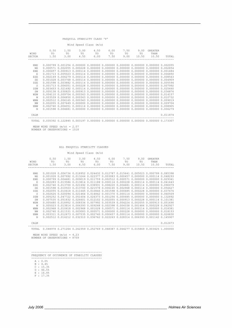
________________________________________________________________________
July 2006 _______________________________________________________________ Holmes Air Sciences
PASQUILL STABILITY CLASS 'F'
Wind Speed Class (m/s)
0.50 1.50 3.00 4.50 6.00 7.50 9.00 GREATER WIND TO TO TO TO TO TO TO THAN SECTOR 1.50 3.00 4.50 6.00 7.50 9.00 10.50 10.50 TOTAL -----------------------------------------------------------------------------------------
NNE 0.000799 0.001256 0.000000 0.000000 0.000000 0.000000 0.000000 0.000000 0.002055 NE 0.000571 0.002055 0.000228 0.000000 0.000000 0.000000 0.000000 0.000000 0.002854 ENE 0.000457 0.000913 0.000114 0.000000 0.000000 0.000000 0.000000 0.000000 0.001484 E 0.001713 0.005023 0.000114 0.000000 0.000000 0.000000 0.000000 0.000000 0.006850 ESE 0.002169 0.006279 0.000114 0.000000 0.000000 0.000000 0.000000 0.000000 0.008563 SE 0.001028 0.003768 0.000114 0.000000 0.000000 0.000000 0.000000 0.000000 0.004909 SSE 0.001598 0.003882 0.000114 0.000000 0.000000 0.000000 0.000000 0.000000 0.005594 S 0.001713 0.006051 0.000228 0.000000 0.000000 0.000000 0.000000 0.000000 0.007992 SSW 0.003653 0.021692 0.000114 0.000000 0.000000 0.000000 0.000000 0.000000 0.025460 SW 0.005138 0.030825 0.000913 0.000000 0.000000 0.000000 0.000000 0.000000 0.036876 WSW 0.004110 0.009704 0.000343 0.000000 0.000000 0.000000 0.000000 0.000000 0.014157 W 0.003539 0.006850 0.000343 0.000000 0.000000 0.000000 0.000000 0.000000 0.010732 WNW 0.002512 0.006165 0.000343 0.000000 0.000000 0.000000 0.000000 0.000000 0.009019 NW 0.002055 0.007649 0.000000 0.000000 0.000000 0.000000 0.000000 0.000000 0.009704 NNW 0.002740 0.006051 0.000114 0.000000 0.000000 0.000000 0.000000 0.000000 0.008905 N 0.001598 0.004681 0.000000 0.000000 0.000000 0.000000 0.000000 0.000000 0.006279
CALM 0.011874 ----------------------------------------------------------------------------------------- TOTAL 0.035392 0.122845 0.003197 0.000000 0.000000 0.000000 0.000000 0.000000 0.173307
MEAN WIND SPEED (m/s) = 2.07 NUMBER OF OBSERVATIONS = 1518
ALL PASQUILL STABILITY CLASSES
Wind Speed Class (m/s)
0.50 1.50 3.00 4.50 6.00 7.50 9.00 GREATER WIND TO TO TO TO TO TO TO THAN SECTOR 1.50 3.00 4.50 6.00 7.50 9.00 10.50 10.50 TOTAL -----------------------------------------------------------------------------------------
NNE 0.001028 0.006736 0.018952 0.024432 0.012787 0.015641 0.005023 0.000799 0.085398 NE 0.001028 0.007992 0.013244 0.022377 0.003083 0.000457 0.000000 0.000114 0.048293 ENE 0.000799 0.004681 0.009019 0.011759 0.002512 0.000571 0.000000 0.000000 0.029341 E 0.002283 0.013586 0.013814 0.011188 0.000114 0.000228 0.000114 0.000114 0.041443 ESE 0.002740 0.013700 0.021692 0.038931 0.008220 0.004681 0.000114 0.000000 0.090079 SE 0.001598 0.010503 0.013700 0.021578 0.006165 0.002968 0.000114 0.000000 0.056627 SSE 0.002055 0.010618 0.011645 0.010846 0.001598 0.000685 0.000228 0.000000 0.037676 S 0.002626 0.020094 0.021464 0.014842 0.001370 0.000114 0.000000 0.000000 0.060509 SSW 0.005252 0.047722 0.051604 0.026373 0.001256 0.000685 0.000000 0.000000 0.132892 SW 0.007535 0.051832 0.026601 0.012102 0.002055 0.000913 0.000228 0.000114 0.101381 WSW 0.005480 0.018952 0.008334 0.007992 0.003539 0.004224 0.002055 0.000913 0.051490 W 0.005023 0.013814 0.006393 0.009248 0.002398 0.004338 0.001484 0.000228 0.042927 WNW 0.002968 0.010618 0.002968 0.001028 0.000571 0.000114 0.000114 0.000000 0.018381 NW 0.002740 0.011531 0.003083 0.000571 0.000000 0.000228 0.000000 0.000000 0.018153 NNW 0.003311 0.012673 0.007535 0.002740 0.000457 0.000114 0.000000 0.000000 0.026830 N 0.002512 0.016212 0.032310 0.036762 0.022263 0.028314 0.006393 0.001142 0.145907
CALM 0.012673 ----------------------------------------------------------------------------------------- TOTAL 0.048978 0.271264 0.262359 0.252769 0.068387 0.064277 0.015869 0.003425 1.000000
MEAN WIND SPEED (m/s) = 4.23 NUMBER OF OBSERVATIONS = 8759
------------------------------------------- FREQUENCY OF OCCURENCE OF STABILITY CLASSES ------------------------------------------- A : 0.0% B : 4.4% C : 15.3% D : 46.5% E : 16.4% F : 17.3%
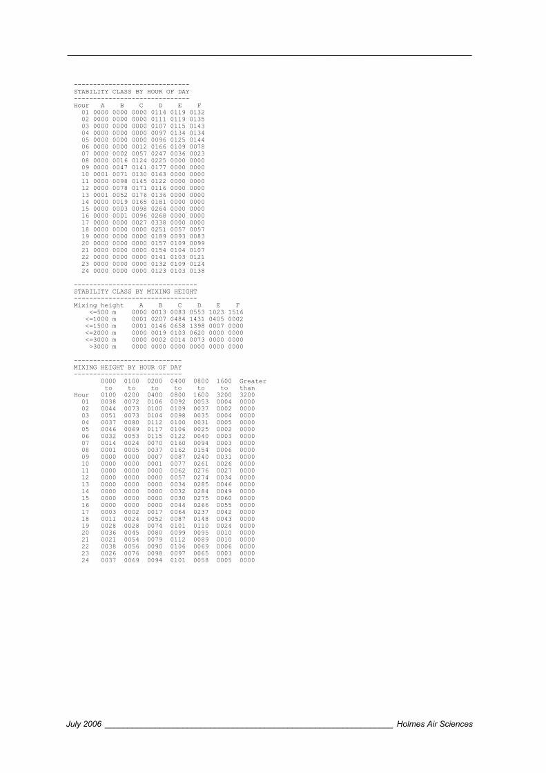
________________________________________________________________________
July 2006 _______________________________________________________________ Holmes Air Sciences
------------------------------ STABILITY CLASS BY HOUR OF DAY ------------------------------ Hour A B C D E F 01 0000 0000 0000 0114 0119 0132 02 0000 0000 0000 0111 0119 0135 03 0000 0000 0000 0107 0115 0143 04 0000 0000 0000 0097 0134 0134 05 0000 0000 0000 0096 0125 0144 06 0000 0000 0012 0166 0109 0078 07 0000 0002 0057 0247 0036 0023 08 0000 0016 0124 0225 0000 0000 09 0000 0047 0141 0177 0000 0000 10 0001 0071 0130 0163 0000 0000 11 0000 0098 0145 0122 0000 0000 12 0000 0078 0171 0116 0000 0000 13 0001 0052 0176 0136 0000 0000 14 0000 0019 0165 0181 0000 0000 15 0000 0003 0098 0264 0000 0000 16 0000 0001 0096 0268 0000 0000 17 0000 0000 0027 0338 0000 0000 18 0000 0000 0000 0251 0057 0057 19 0000 0000 0000 0189 0093 0083 20 0000 0000 0000 0157 0109 0099 21 0000 0000 0000 0154 0104 0107 22 0000 0000 0000 0141 0103 0121 23 0000 0000 0000 0132 0109 0124 24 0000 0000 0000 0123 0103 0138
-------------------------------- STABILITY CLASS BY MIXING HEIGHT -------------------------------- Mixing height A B C D E F <=500 m 0000 0013 0083 0553 1023 1516 <=1000 m 0001 0207 0484 1431 0405 0002 <=1500 m 0001 0146 0658 1398 0007 0000 <=2000 m 0000 0019 0103 0620 0000 0000 <=3000 m 0000 0002 0014 0073 0000 0000 >3000 m 0000 0000 0000 0000 0000 0000
---------------------------- MIXING HEIGHT BY HOUR OF DAY ---------------------------- 0000 0100 0200 0400 0800 1600 Greater to to to to to to than Hour 0100 0200 0400 0800 1600 3200 3200 01 0038 0072 0106 0092 0053 0004 0000 02 0044 0073 0100 0109 0037 0002 0000 03 0051 0073 0104 0098 0035 0004 0000 04 0037 0080 0112 0100 0031 0005 0000 05 0046 0069 0117 0106 0025 0002 0000 06 0032 0053 0115 0122 0040 0003 0000 07 0014 0024 0070 0160 0094 0003 0000 08 0001 0005 0037 0162 0154 0006 0000 09 0000 0000 0007 0087 0240 0031 0000 10 0000 0000 0001 0077 0261 0026 0000 11 0000 0000 0000 0062 0276 0027 0000 12 0000 0000 0000 0057 0274 0034 0000 13 0000 0000 0000 0034 0285 0046 0000 14 0000 0000 0000 0032 0284 0049 0000 15 0000 0000 0000 0030 0275 0060 0000 16 0000 0000 0000 0044 0266 0055 0000 17 0003 0002 0017 0064 0237 0042 0000 18 0011 0024 0052 0087 0148 0043 0000 19 0028 0028 0074 0101 0110 0024 0000 20 0036 0045 0080 0099 0095 0010 0000 21 0021 0054 0079 0112 0089 0010 0000 22 0038 0056 0090 0106 0069 0006 0000 23 0026 0076 0098 0097 0065 0003 0000 24 0037 0069 0094 0101 0058 0005 0000
________________________________________________________________________
July 2006 _______________________________________________________________ Holmes Air Sciences
APPENDIX C VEHICLE EMISSION ESTIMATES
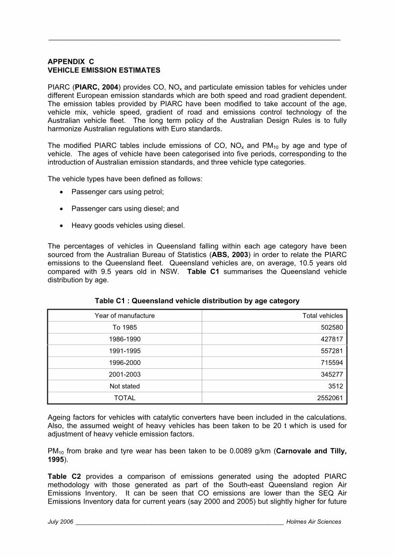
________________________________________________________________________
July 2006 _______________________________________________________________ Holmes Air Sciences
APPENDIX C VEHICLE EMISSION ESTIMATES
PIARC (PIARC, 2004) provides CO, NOx and particulate emission tables for vehicles under different European emission standards which are both speed and road gradient dependent. The emission tables provided by PIARC have been modified to take account of the age, vehicle mix, vehicle speed, gradient of road and emissions control technology of the Australian vehicle fleet. The long term policy of the Australian Design Rules is to fully harmonize Australian regulations with Euro standards.
The modified PIARC tables include emissions of CO, NOx and PM10 by age and type of vehicle. The ages of vehicle have been categorised into five periods, corresponding to the introduction of Australian emission standards, and three vehicle type categories.
The vehicle types have been defined as follows:
Passenger cars using petrol;
Passenger cars using diesel; and
Heavy goods vehicles using diesel.
The percentages of vehicles in Queensland falling within each age category have been sourced from the Australian Bureau of Statistics (ABS, 2003) in order to relate the PIARC emissions to the Queensland fleet. Queensland vehicles are, on average, 10.5 years old compared with 9.5 years old in NSW. Table C1 summarises the Queensland vehicle distribution by age.
Table C1 : Queensland vehicle distribution by age category
Year of manufacture Total vehicles
To 1985 502580
1986-1990 427817
1991-1995 557281
1996-2000 715594
2001-2003 345277
Not stated 3512
TOTAL 2552061
Ageing factors for vehicles with catalytic converters have been included in the calculations. Also, the assumed weight of heavy vehicles has been taken to be 20 t which is used for adjustment of heavy vehicle emission factors.
PM10 from brake and tyre wear has been taken to be 0.0089 g/km (Carnovale and Tilly, 1995).
Table C2 provides a comparison of emissions generated using the adopted PIARC methodology with those generated as part of the South-east Queensland region Air Emissions Inventory. It can be seen that CO emissions are lower than the SEQ Air Emissions Inventory data for current years (say 2000 and 2005) but slightly higher for future
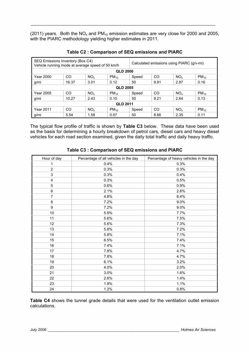
________________________________________________________________________
July 2006 _______________________________________________________________ Holmes Air Sciences
(2011) years. Both the NOx and PM10 emission estimates are very close for 2000 and 2005, with the PIARC methodology yielding higher estimates in 2011.
Table C2 : Comparison of SEQ emissions and PIARC
SEQ Emissions Inventory (Box C4) Vehicle running mode at average speed of 50 km/h Calculated emissions using PIARC (g/v-mi)
QLD 2000 Year 2000 CO NOx PM10 Speed CO NOx PM10
g/mi 16.37 3.01 0.12 50 9.91 2.87 0.16 QLD 2005
Year 2005 CO NOx PM10 Speed CO NOx PM10
g/mi 10.27 2.43 0.10 50 9.21 2.64 0.13 QLD 2011
Year 2011 CO NOx PM10 Speed CO NOx PM10
g/mi 5.54 1.58 0.07 50 8.66 2.35 0.11
The typical flow profile of traffic is shown by Table C3 below. These data have been used as the basis for determining a hourly breakdown of petrol cars, diesel cars and heavy diesel vehicles for each road section examined, given the daily total traffic and daily heavy traffic.
Table C3 : Comparison of SEQ emissions and PIARC
Hour of day Percentage of all vehicles in the day Percentage of heavy vehicles in the day 1 0.4% 0.3% 2 0.3% 0.3% 3 0.3% 0.4% 4 0.3% 0.5% 5 0.6% 0.9% 6 2.1% 2.6% 7 4.8% 6.4% 8 7.2% 9.0% 9 7.2% 9.0%
10 5.9% 7.7% 11 5.6% 7.5% 12 5.6% 7.3% 13 5.8% 7.2% 14 5.8% 7.1% 15 6.5% 7.4% 16 7.4% 7.1% 17 7.8% 4.7% 18 7.8% 4.7% 19 6.1% 3.2% 20 4.0% 2.0% 21 3.0% 1.6% 22 2.6% 1.4% 23 1.9% 1.1% 24 1.2% 0.8%
Table C4 shows the tunnel grade details that were used for the ventilation outlet emission calculations.
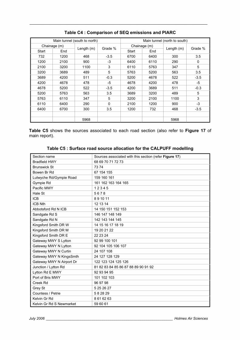
________________________________________________________________________
July 2006 _______________________________________________________________ Holmes Air Sciences
Table C4 : Comparison of SEQ emissions and PIARC
Main tunnel (south to north) Main tunnel (north to south) Chainage (m) Chainage (m)
Start End Length (m) Grade %
Start End Length (m) Grade %
732 1200 468 -3.5 6700 6400 300 3.5 1200 2100 900 -3 6400 6110 290 0 2100 3200 1100 3 6110 5763 347 5 3200 3689 489 5 5763 5200 563 3.5 3689 4200 511 -0.3 5200 4678 522 -3.5 4200 4678 478 -5 4678 4200 478 -5 4678 5200 522 -3.5 4200 3689 511 -0.3 5200 5763 563 3.5 3689 3200 489 5 5763 6110 347 5 3200 2100 1100 3 6110 6400 290 0 2100 1200 900 -3 6400 6700 300 3.5 1200 732 468 -3.5
5968 5968
Table C5 shows the sources associated to each road section (also refer to Figure 17 of main report).
Table C5 : Surface road source allocation for the CALPUFF modelling
Section name Sources associated with this section (refer Figure 17)Bradfield HWY 68 69 70 71 72 73 Brunswick St 73 74 Bowen Br Rd 67 154 155 Lutwyche Rd/Gympie Road 159 160 161 Gympie Rd 161 162 163 164 165 Pacific MWY 1 2 3 4 5 Hale St 5 6 7 8 ICB 8 9 10 11 ICB Nth 12 13 14 Abbotsford Rd N ICB 14 150 151 152 153 Sandgate Rd S 146 147 148 149 Sandgate Rd N 142 143 144 145 Kingsford Smith DR W 14 15 16 17 18 19 Kingsford Smith DR M 19 20 21 22 Kingsford Smith DR E 22 23 24 Gateway MWY S Lytton 92 99 100 101 Gateway MWY N Lytton 92 104 105 106 107 Gateway MWY N Curtin 24 107 108 Gateway MWY N KingsSmth 24 127 128 129 Gateway MWY N Airport Dr 122 123 124 125 126 Junction / Lytton Rd 81 82 83 84 85 86 87 88 89 90 91 92 Lytton Rd E MWY 92 93 94 95 Port of Bris MWY 101 102 103 Creek Rd 96 97 98 Grey St 5 25 26 27 Countess / Petrie 5 8 28 29 Kelvin Gr Rd 8 61 62 63 Kelvin Gr Rd S Newmarket 59 60 61
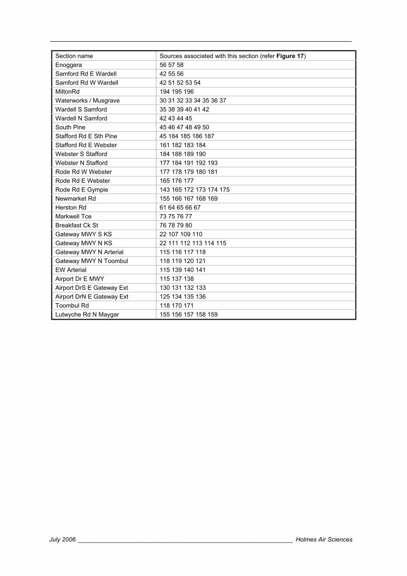
________________________________________________________________________
July 2006 _______________________________________________________________ Holmes Air Sciences
Section name Sources associated with this section (refer Figure 17)Enoggera 56 57 58 Samford Rd E Wardell 42 55 56 Samford Rd W Wardell 42 51 52 53 54 MiltonRd 194 195 196 Waterworks / Musgrave 30 31 32 33 34 35 36 37 Wardell S Samford 35 38 39 40 41 42 Wardell N Samford 42 43 44 45 South Pine 45 46 47 48 49 50 Stafford Rd E Sth Pine 45 184 185 186 187 Stafford Rd E Webster 161 182 183 184 Webster S Stafford 184 188 189 190 Webster N Stafford 177 184 191 192 193 Rode Rd W Webster 177 178 179 180 181 Rode Rd E Webster 165 176 177 Rode Rd E Gympie 143 165 172 173 174 175 Newmarket Rd 155 166 167 168 169 Herston Rd 61 64 65 66 67 Markwell Tce 73 75 76 77 Breakfast Ck St 76 78 79 80 Gateway MWY S KS 22 107 109 110 Gateway MWY N KS 22 111 112 113 114 115 Gateway MWY N Arterial 115 116 117 118 Gateway MWY N Toombul 118 119 120 121 EW Arterial 115 139 140 141 Airport Dr E MWY 115 137 138 Airport DrS E Gateway Ext 130 131 132 133 Airport DrN E Gateway Ext 125 134 135 136 Toombul Rd 118 170 171 Lutwyche Rd N Maygar 155 156 157 158 159

________________________________________________________________________
July 2006 _______________________________________________________________ Holmes Air Sciences
FIGURES
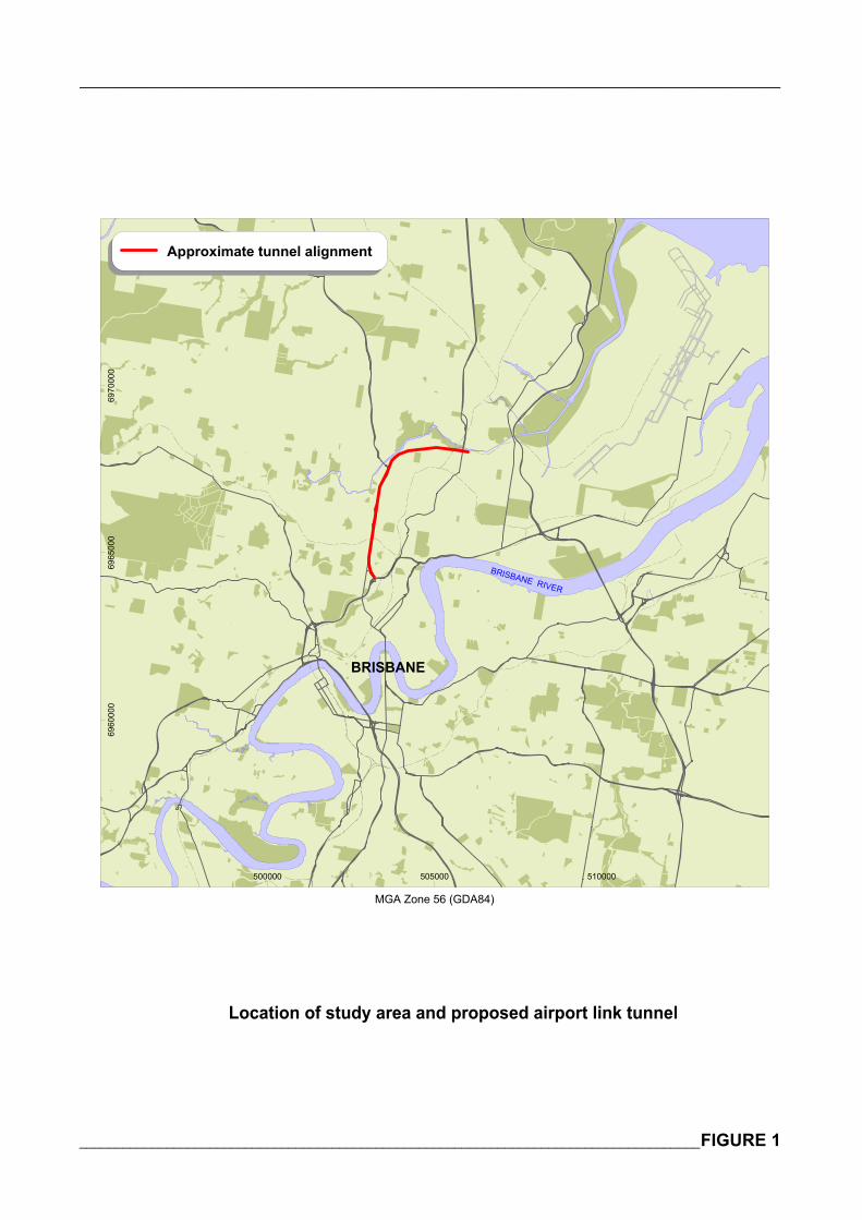
_______________________________________________________________________________
______________________________________________________________________________________FIGURE 1
500000 505000 510000
MGA Zone 56 (GDA84)
6960
000
6965
000
6970
000
Location of study area and proposed airport link tunnel
Approximate tunnel alignment
BRISBANE RIVER
BRISBANE
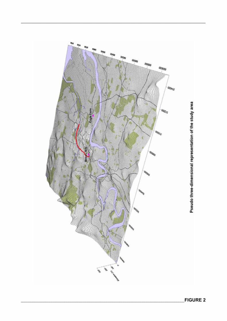
_______________________________________________________________________________
______________________________________________________________________________________FIGURE 2
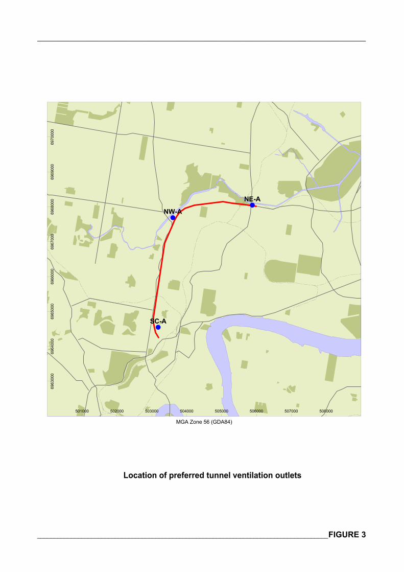
_______________________________________________________________________________
______________________________________________________________________________________FIGURE 3
501000 502000 503000 504000 505000 506000 507000 508000
MGA Zone 56 (GDA84)
6963
000
6964
000
6965
000
6966
000
6967
000
6968
000
6969
000
6970
000
SC-A
NW-A
NE-A
Location of preferred tunnel ventilation outlets
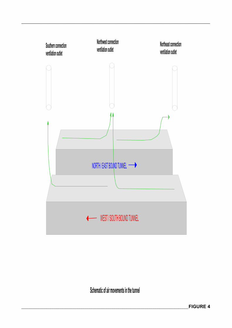
_______________________________________________________________________________
______________________________________________________________________________________FIGURE 4
WEST / SOUTH BOUND TUNNEL
NORTH / EAST BOUND TUNNEL
Schematic of air movements in the tunnel
Southern connection ventilation outlet
Northwest connection ventilation outlet
Northeast connection ventilation outlet
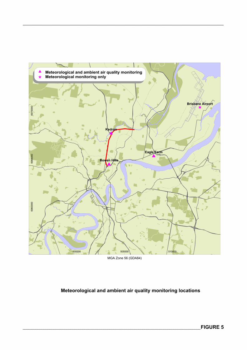
_______________________________________________________________________________
______________________________________________________________________________________FIGURE 5
500000 505000 510000
MGA Zone 56 (GDA84)
6960
000
6965
000
6970
000
Bowen Hills
Eagle Farm
Kedron
Brisbane Airport
Meteorological and ambient air quality monitoring locations
Meteorological and ambient air quality monitoringMeteorological monitoring only
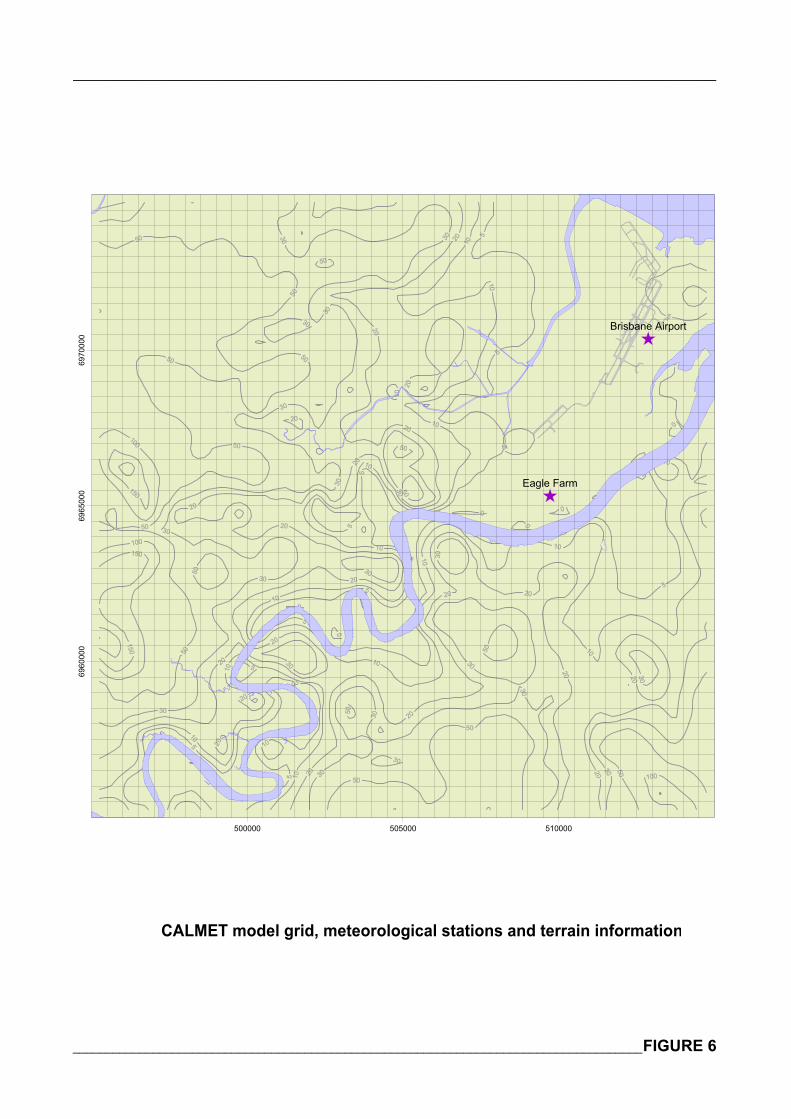
_______________________________________________________________________________
______________________________________________________________________________________FIGURE 6
500000 505000 510000
6960
000
6965
000
6970
000
Eagle Farm
Brisbane Airport
CALMET model grid, meteorological stations and terrain information
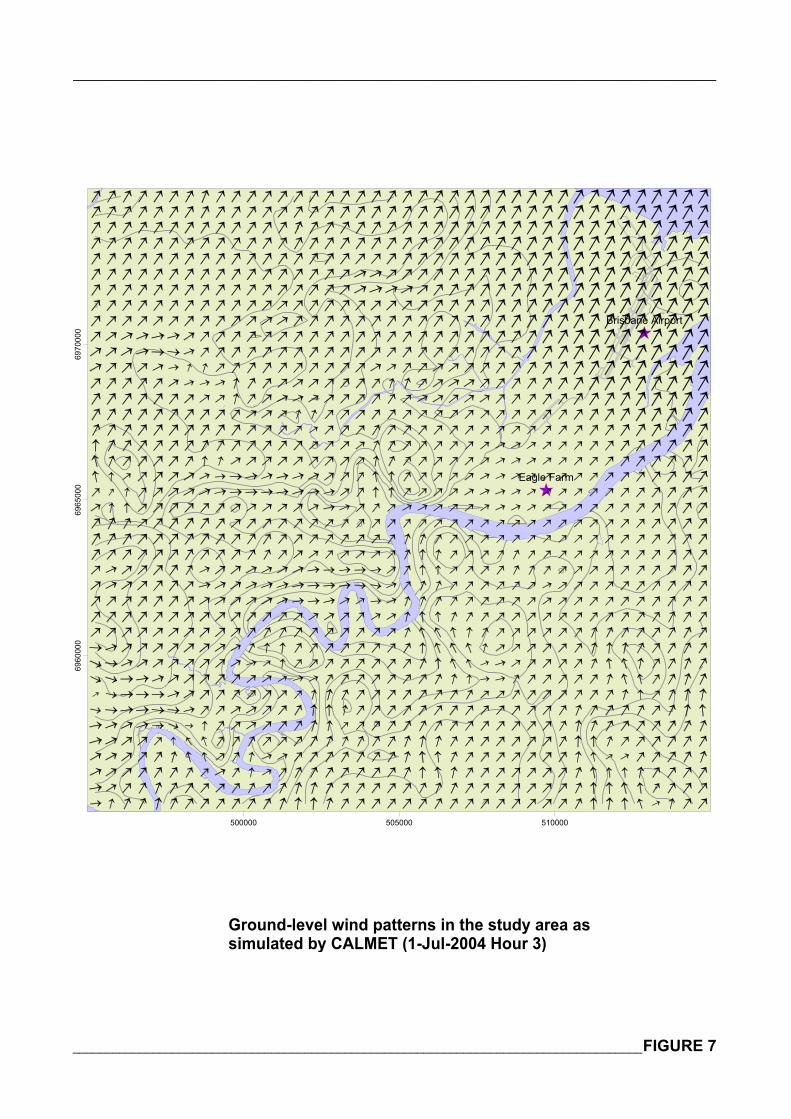
_______________________________________________________________________________
______________________________________________________________________________________FIGURE 7
500000 505000 510000
6960
000
6965
000
6970
000
Eagle Farm
Brisbane Airport
Ground-level wind patterns in the study area as simulated by CALMET (1-Jul-2004 Hour 3)
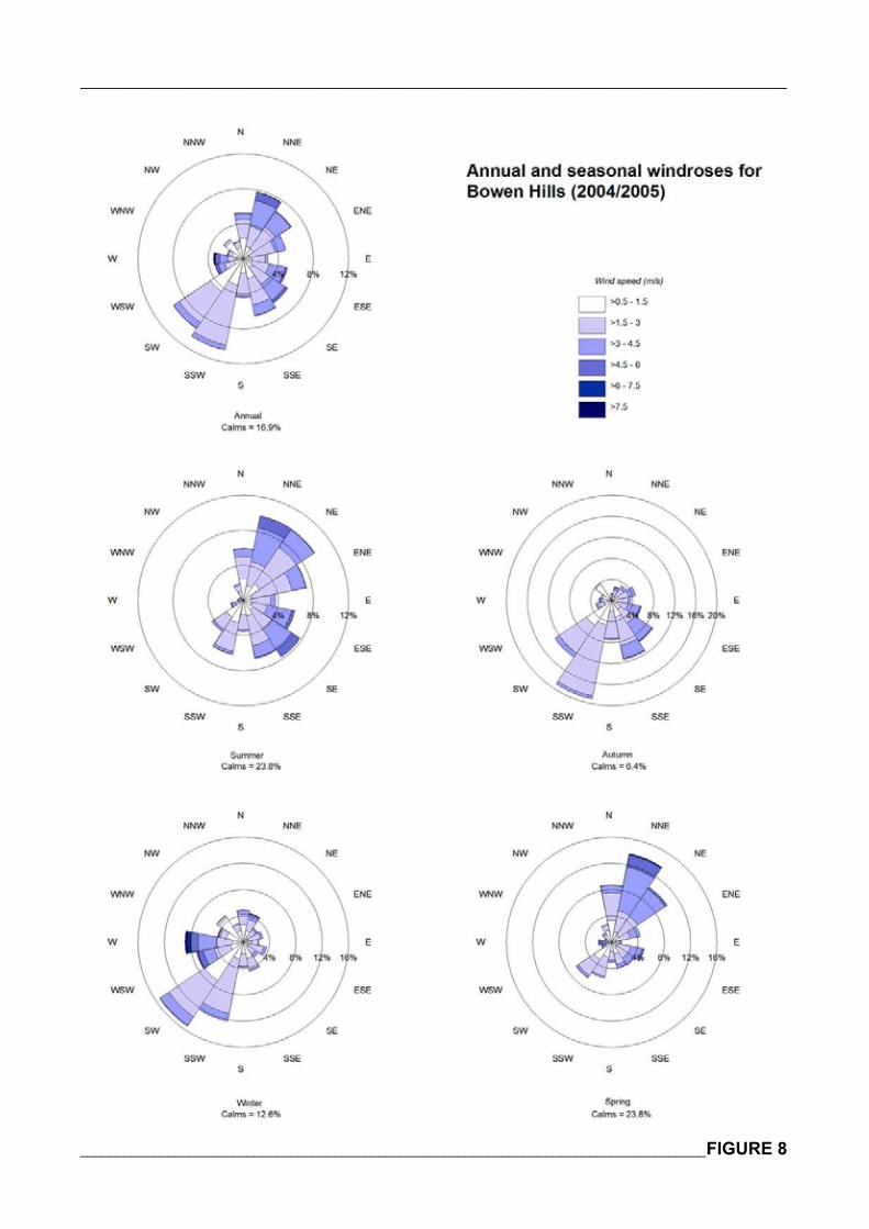
_______________________________________________________________________________
______________________________________________________________________________________FIGURE 8
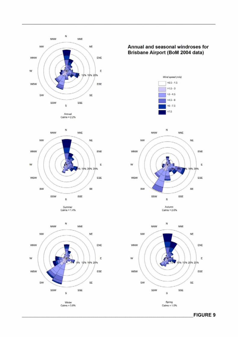
_______________________________________________________________________________
______________________________________________________________________________________FIGURE 9
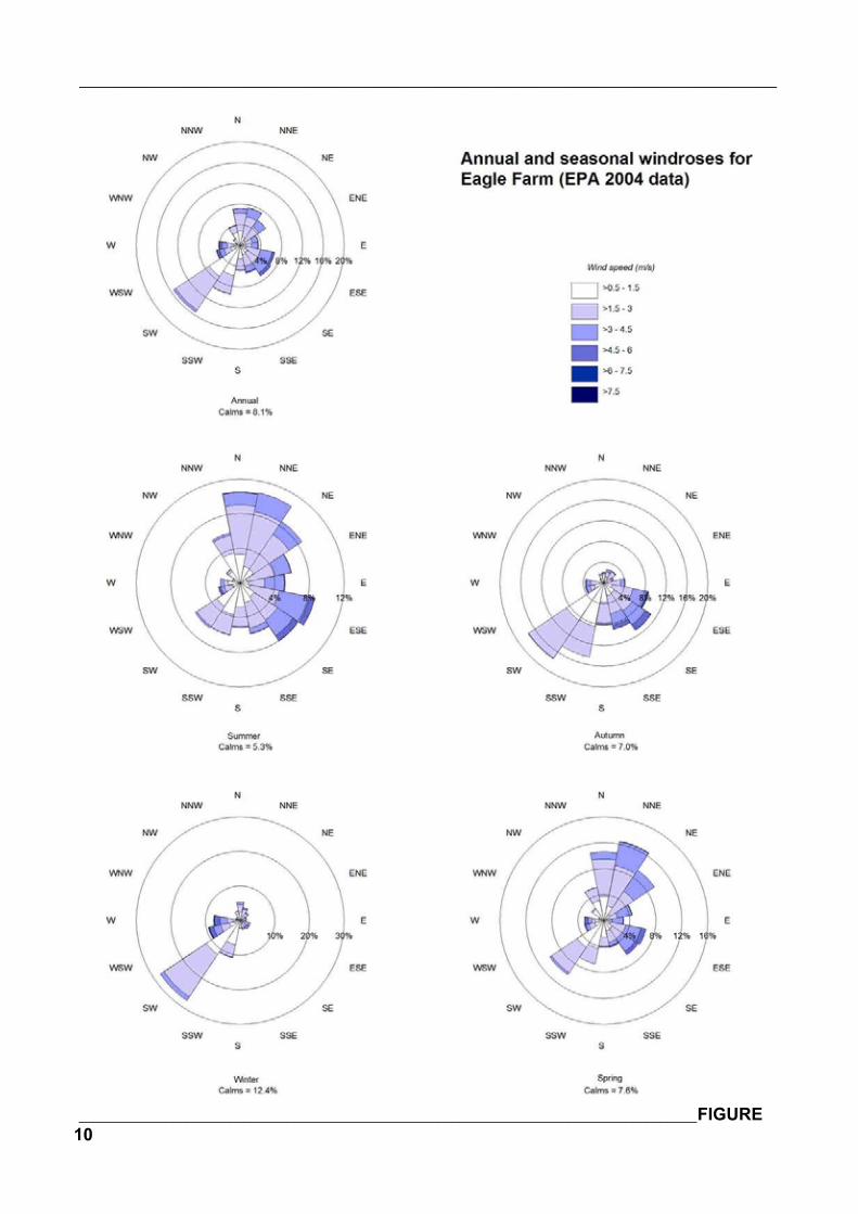
_______________________________________________________________________________
______________________________________________________________________________________FIGURE10
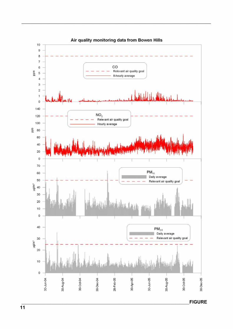
_______________________________________________________________________________
______________________________________________________________________________________FIGURE11
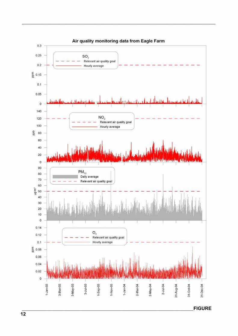
_______________________________________________________________________________
______________________________________________________________________________________FIGURE12
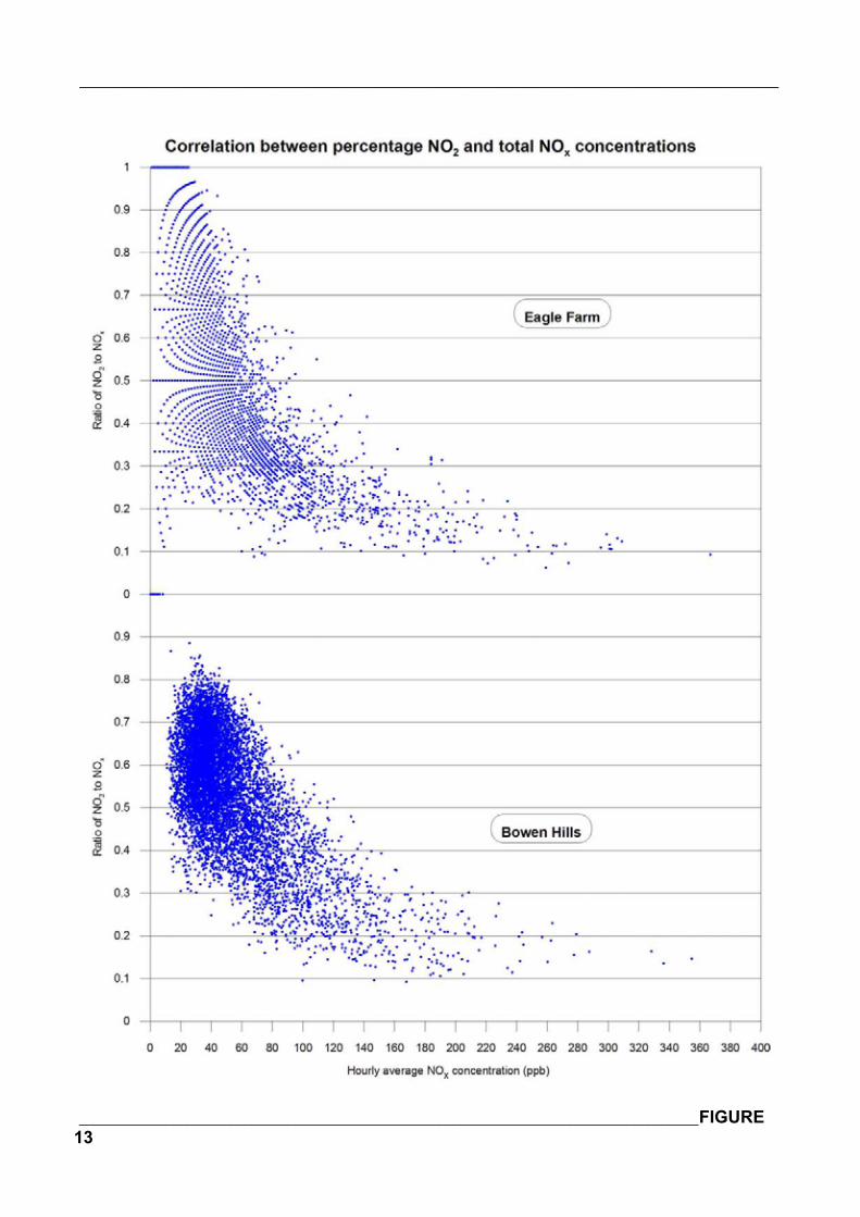
_______________________________________________________________________________
______________________________________________________________________________________FIGURE13
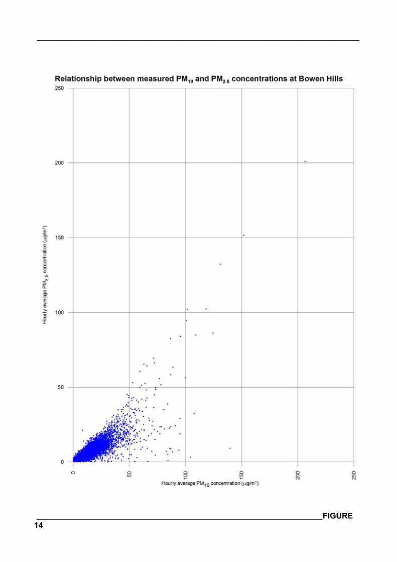
_______________________________________________________________________________
______________________________________________________________________________________FIGURE14
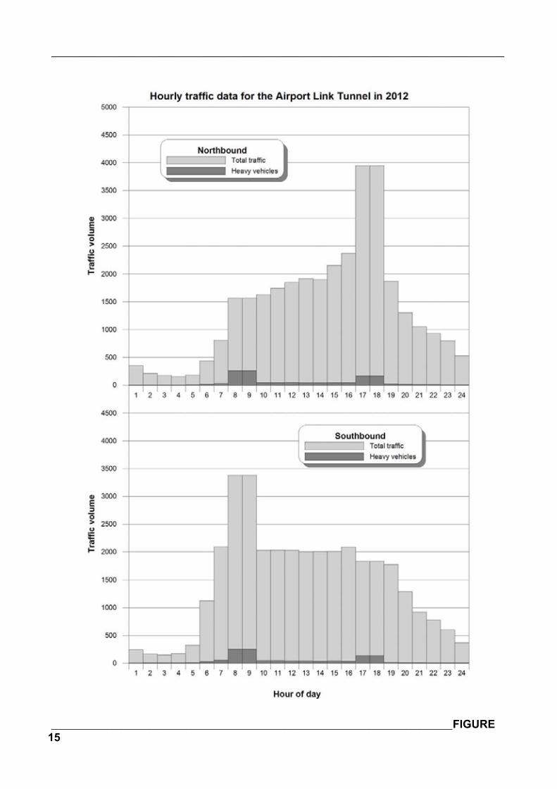
_______________________________________________________________________________
______________________________________________________________________________________FIGURE15
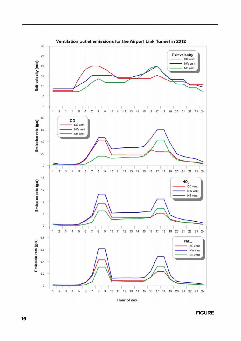
_______________________________________________________________________________
______________________________________________________________________________________FIGURE16
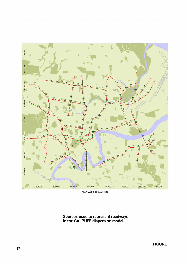
_______________________________________________________________________________
______________________________________________________________________________________FIGURE17
498000 500000 502000 504000 506000 508000 510000 512000
MGA Zone 56 (GDA84)
6960
000
6962
000
6964
000
6966
000
6968
000
6970
000
6972
000
6974
000
1
2
3
456
7
8 9
10
1112
1314
15 16 17 18 1920
2122
2324
25
26
27
28
29
3031
32
333435
3637
38
39
40
41
42
43
44
45
46
47
48
4950
5152
53
54
5556
57
58
59
60
61
62
63
6465 66 67
68
69
70
71
72
7374 75
76
77
78
79
80
8182
8384
8586
87
88 89 90 91 92
93
94
95
96
97
98
99
100
101
102
103104
105
106
107
108109110
111
112
113
114
115
116
117
118
119
120121
122
123
124
125
126
127
128
129
130
131
132133
134
135
136
137138139140141
142
143
144
145
146
147
148
149150
151
152
153
154
155
156
157
158
159
160
161
162
163
164
165
166167168169
170
171
172173174175176177178179180181
182183184185186187
188
189
190
191
192
193
194195
196
Sources used to represent roadwaysin the CALPUFF dispersion model
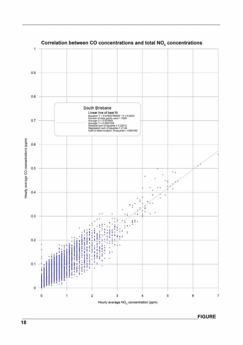
_______________________________________________________________________________
______________________________________________________________________________________FIGURE18
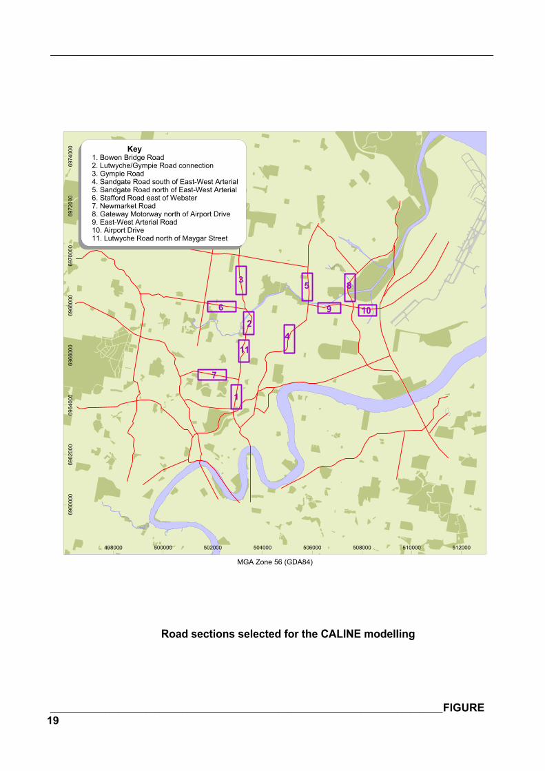
_______________________________________________________________________________
______________________________________________________________________________________FIGURE19
498000 500000 502000 504000 506000 508000 510000 512000
MGA Zone 56 (GDA84)
6960
000
6962
000
6964
000
6966
000
6968
000
6970
000
6972
000
6974
000
Road sections selected for the CALINE modelling
1
2
3
4
5
9
8
106
7
Key1. Bowen Bridge Road2. Lutwyche/Gympie Road connection3. Gympie Road4. Sandgate Road south of East-West Arterial5. Sandgate Road north of East-West Arterial6. Stafford Road east of Webster7. Newmarket Road8. Gateway Motorway north of Airport Drive9. East-West Arterial Road10. Airport Drive11. Lutwyche Road north of Maygar Street
11
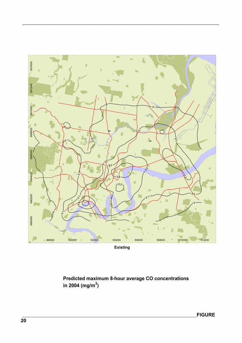
_______________________________________________________________________________
______________________________________________________________________________________FIGURE20
498000 500000 502000 504000 506000 508000 510000 512000
Existing
6960
000
6962
000
6964
000
6966
000
6968
000
6970
000
6972
000
6974
000
Predicted maximum 8-hour average CO concentrationsin 2004 (mg/m3)
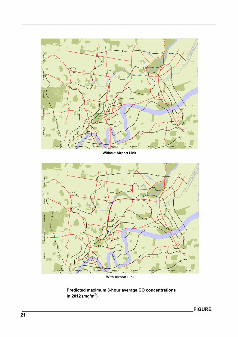
_______________________________________________________________________________
______________________________________________________________________________________FIGURE21
498000 500000 502000 504000 506000 508000 510000 512000
With Airport Link
6962
000
6964
000
6966
000
6968
000
6970
000
498000 500000 502000 504000 506000 508000 510000 512000
Without Airport Link
6962
000
6964
000
6966
000
6968
000
6970
000
Predicted maximum 8-hour average CO concentrationsin 2012 (mg/m3)
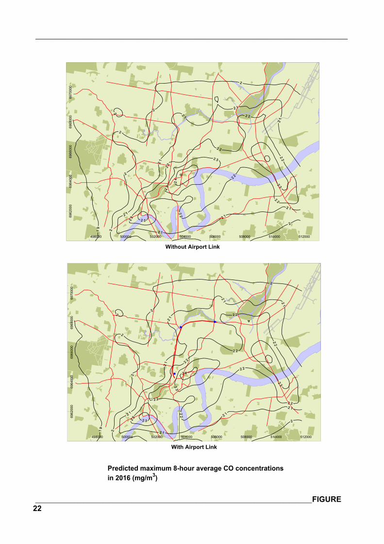
_______________________________________________________________________________
______________________________________________________________________________________FIGURE22
498000 500000 502000 504000 506000 508000 510000 512000
With Airport Link
6962
000
6964
000
6966
000
6968
000
6970
000
498000 500000 502000 504000 506000 508000 510000 512000
Without Airport Link
6962
000
6964
000
6966
000
6968
000
6970
000
Predicted maximum 8-hour average CO concentrationsin 2016 (mg/m3)
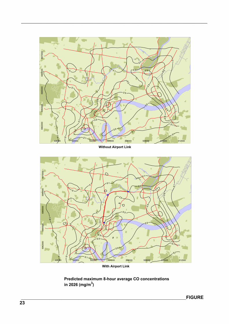
_______________________________________________________________________________
______________________________________________________________________________________FIGURE23
498000 500000 502000 504000 506000 508000 510000 512000
With Airport Link
6962
000
6964
000
6966
000
6968
000
6970
000
498000 500000 502000 504000 506000 508000 510000 512000
Without Airport Link
6962
000
6964
000
6966
000
6968
000
6970
000
Predicted maximum 8-hour average CO concentrationsin 2026 (mg/m3)
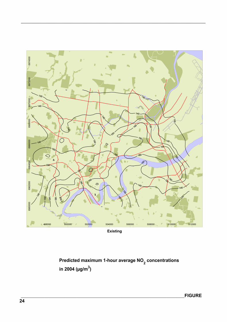
_______________________________________________________________________________
______________________________________________________________________________________FIGURE24
498000 500000 502000 504000 506000 508000 510000 512000
Existing
6960
000
6962
000
6964
000
6966
000
6968
000
6970
000
6972
000
6974
000
Predicted maximum 1-hour average NO2 concentrations
in 2004 (µg/m3)
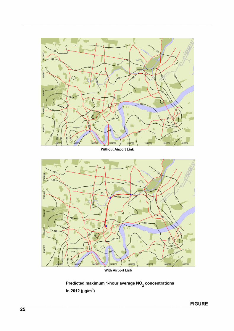
_______________________________________________________________________________
______________________________________________________________________________________FIGURE25
498000 500000 502000 504000 506000 508000 510000 512000
With Airport Link
6962
000
6964
000
6966
000
6968
000
6970
000
498000 500000 502000 504000 506000 508000 510000 512000
Without Airport Link
6962
000
6964
000
6966
000
6968
000
6970
000
Predicted maximum 1-hour average NO2 concentrations
in 2012 (µg/m3)
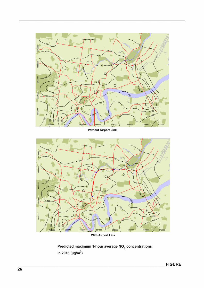
_______________________________________________________________________________
______________________________________________________________________________________FIGURE26
498000 500000 502000 504000 506000 508000 510000 512000
With Airport Link
6962
000
6964
000
6966
000
6968
000
6970
000
498000 500000 502000 504000 506000 508000 510000 512000
Without Airport Link
6962
000
6964
000
6966
000
6968
000
6970
000
Predicted maximum 1-hour average NO2 concentrations
in 2016 (µg/m3)

_______________________________________________________________________________
______________________________________________________________________________________FIGURE27
498000 500000 502000 504000 506000 508000 510000 512000
With Airport Link
6962
000
6964
000
6966
000
6968
000
6970
000
498000 500000 502000 504000 506000 508000 510000 512000
Without Airport Link
6962
000
6964
000
6966
000
6968
000
6970
000
Predicted maximum 1-hour average NO2 concentrations
in 2026 (µg/m3)
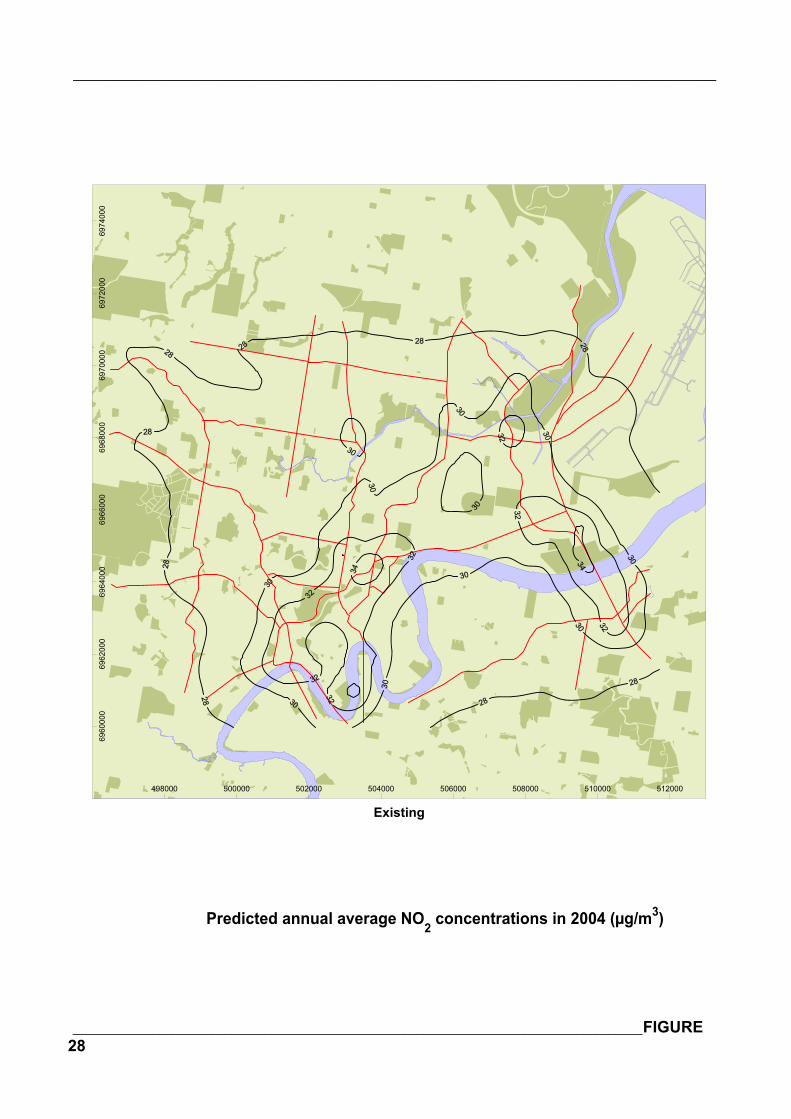
_______________________________________________________________________________
______________________________________________________________________________________FIGURE28
498000 500000 502000 504000 506000 508000 510000 512000
Existing
6960
000
6962
000
6964
000
6966
000
6968
000
6970
000
6972
000
6974
000
Predicted annual average NO2 concentrations in 2004 (µg/m3)
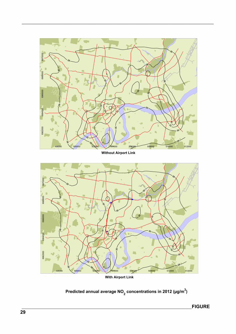
_______________________________________________________________________________
______________________________________________________________________________________FIGURE29
498000 500000 502000 504000 506000 508000 510000 512000
With Airport Link
6962
000
6964
000
6966
000
6968
000
6970
000
498000 500000 502000 504000 506000 508000 510000 512000
Without Airport Link
6962
000
6964
000
6966
000
6968
000
6970
000
Predicted annual average NO2 concentrations in 2012 (µg/m3)

_______________________________________________________________________________
______________________________________________________________________________________FIGURE30
498000 500000 502000 504000 506000 508000 510000 512000
With Airport Link
6962
000
6964
000
6966
000
6968
000
6970
000
498000 500000 502000 504000 506000 508000 510000 512000
Without Airport Link
6962
000
6964
000
6966
000
6968
000
6970
000
Predicted annual average NO2 concentrations in 2016 (µg/m3)
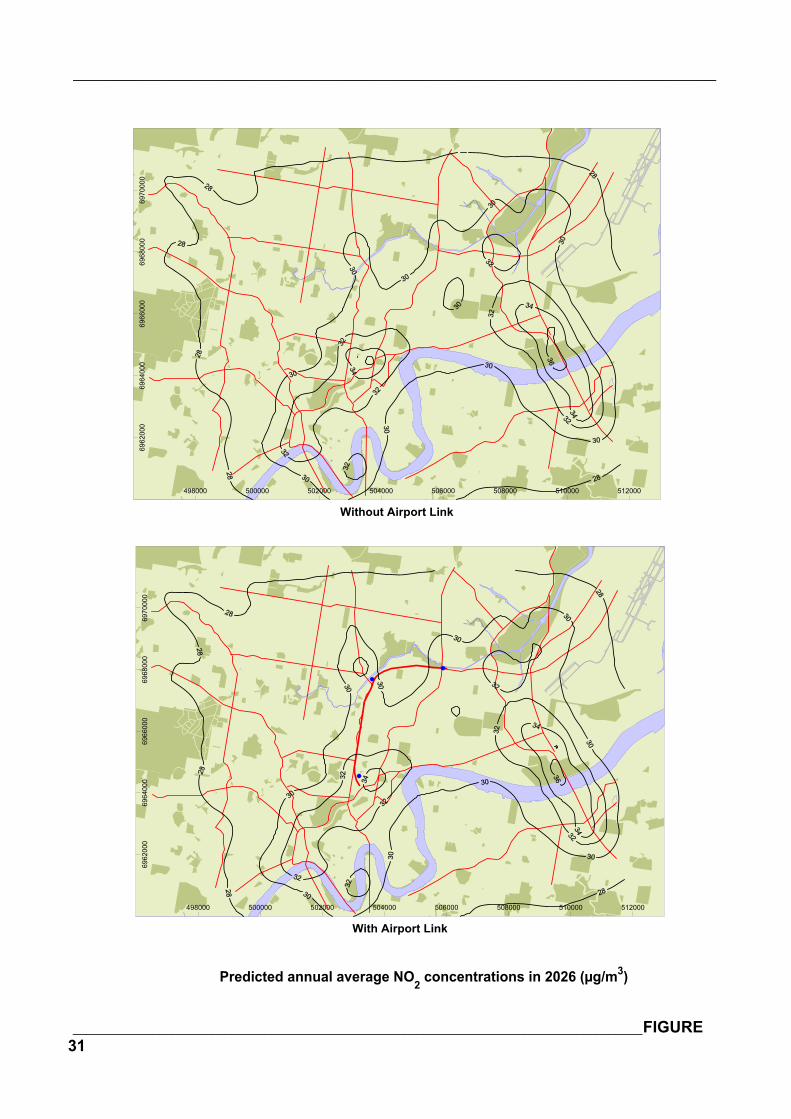
_______________________________________________________________________________
______________________________________________________________________________________FIGURE31
498000 500000 502000 504000 506000 508000 510000 512000
With Airport Link
6962
000
6964
000
6966
000
6968
000
6970
000
498000 500000 502000 504000 506000 508000 510000 512000
Without Airport Link
6962
000
6964
000
6966
000
6968
000
6970
000
Predicted annual average NO2 concentrations in 2026 (µg/m3)
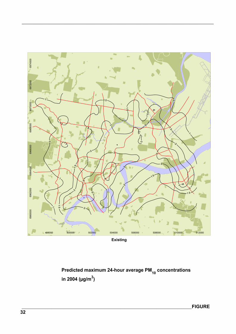
_______________________________________________________________________________
______________________________________________________________________________________FIGURE32
498000 500000 502000 504000 506000 508000 510000 512000
Existing
6960
000
6962
000
6964
000
6966
000
6968
000
6970
000
6972
000
6974
000
Predicted maximum 24-hour average PM10 concentrations
in 2004 (µg/m3)
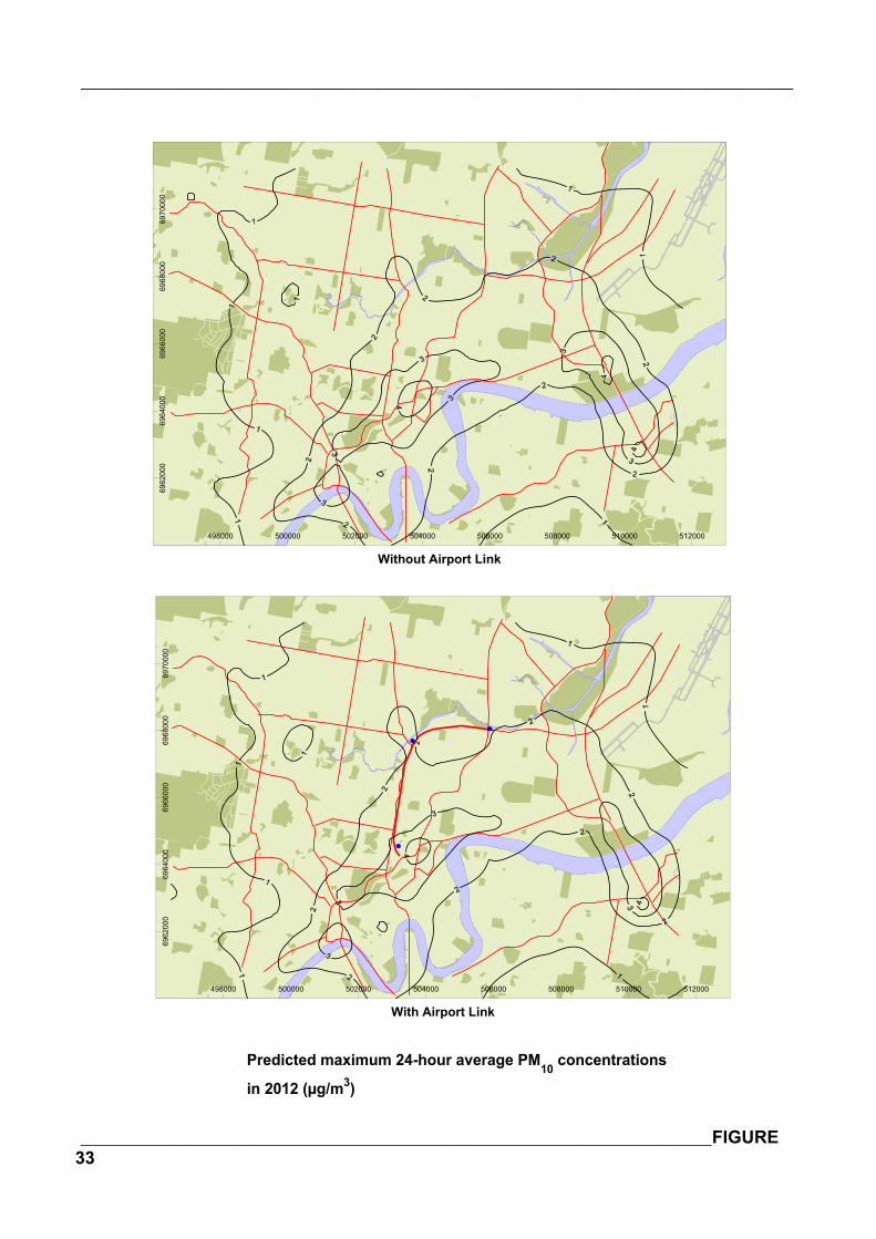
_______________________________________________________________________________
______________________________________________________________________________________FIGURE33
498000 500000 502000 504000 506000 508000 510000 512000
With Airport Link
6962
000
6964
000
6966
000
6968
000
6970
000
498000 500000 502000 504000 506000 508000 510000 512000
Without Airport Link
6962
000
6964
000
6966
000
6968
000
6970
000
Predicted maximum 24-hour average PM10 concentrations
in 2012 (µg/m3)

_______________________________________________________________________________
______________________________________________________________________________________FIGURE34
498000 500000 502000 504000 506000 508000 510000 512000
With Airport Link
6962
000
6964
000
6966
000
6968
000
6970
000
498000 500000 502000 504000 506000 508000 510000 512000
Without Airport Link
6962
000
6964
000
6966
000
6968
000
6970
000
Predicted maximum 24-hour average PM10 concentrations
in 2016 (µg/m3)
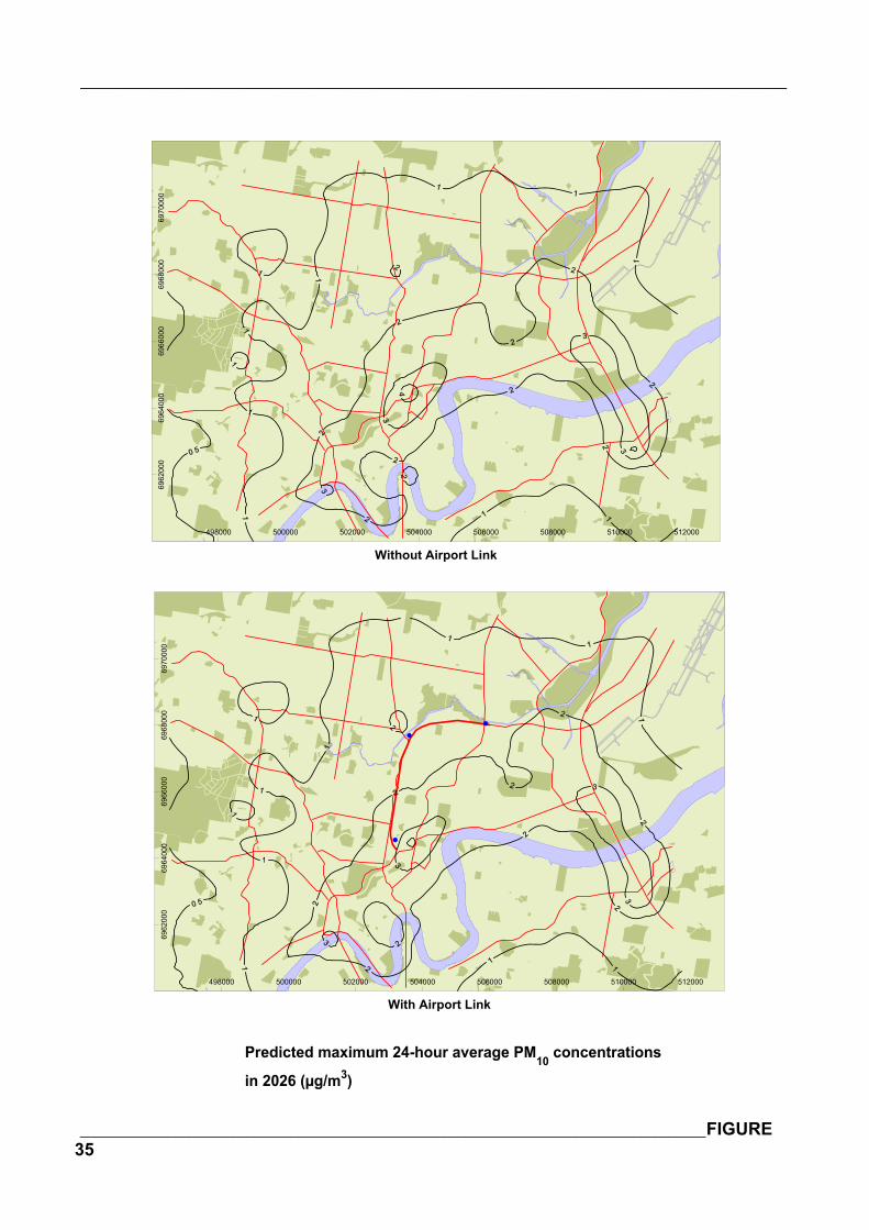
_______________________________________________________________________________
______________________________________________________________________________________FIGURE35
498000 500000 502000 504000 506000 508000 510000 512000
With Airport Link
6962
000
6964
000
6966
000
6968
000
6970
000
498000 500000 502000 504000 506000 508000 510000 512000
Without Airport Link
6962
000
6964
000
6966
000
6968
000
6970
000
Predicted maximum 24-hour average PM10 concentrations
in 2026 (µg/m3)
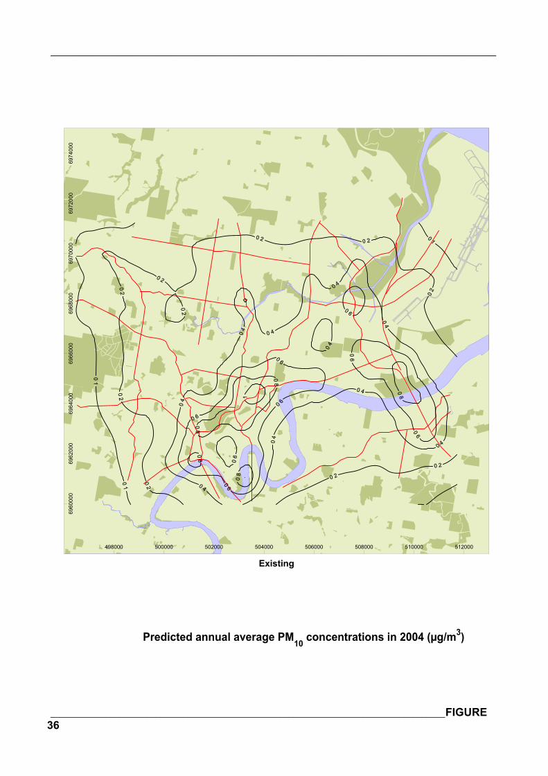
_______________________________________________________________________________
______________________________________________________________________________________FIGURE36
498000 500000 502000 504000 506000 508000 510000 512000
Existing
6960
000
6962
000
6964
000
6966
000
6968
000
6970
000
6972
000
6974
000
Predicted annual average PM10 concentrations in 2004 (µg/m3)
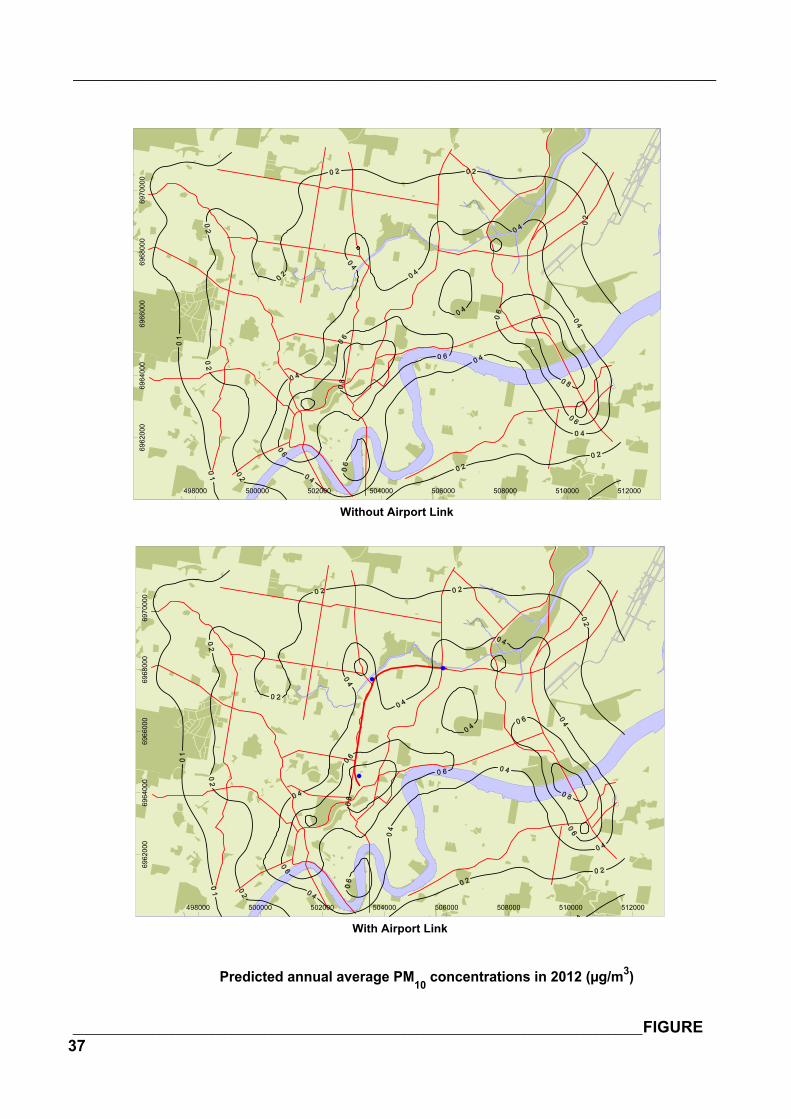
_______________________________________________________________________________
______________________________________________________________________________________FIGURE37
498000 500000 502000 504000 506000 508000 510000 512000
With Airport Link
6962
000
6964
000
6966
000
6968
000
6970
000
498000 500000 502000 504000 506000 508000 510000 512000
Without Airport Link
6962
000
6964
000
6966
000
6968
000
6970
000
Predicted annual average PM10 concentrations in 2012 (µg/m3)
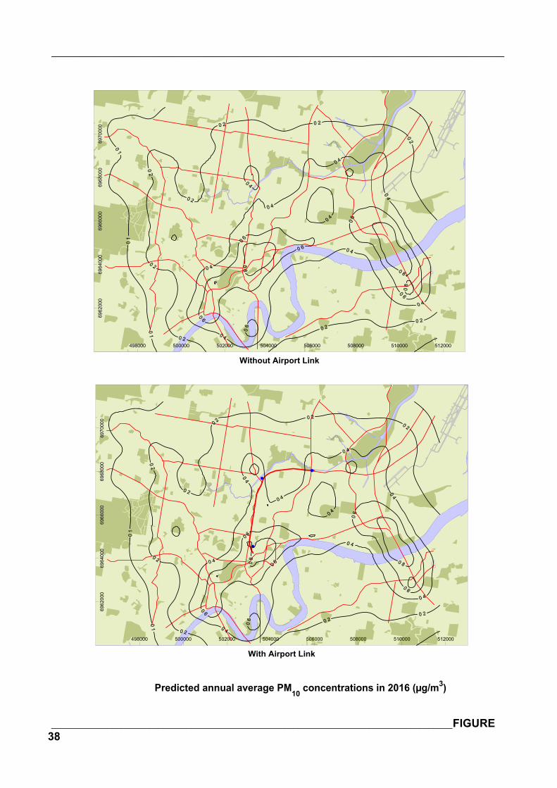
_______________________________________________________________________________
______________________________________________________________________________________FIGURE38
498000 500000 502000 504000 506000 508000 510000 512000
With Airport Link
6962
000
6964
000
6966
000
6968
000
6970
000
498000 500000 502000 504000 506000 508000 510000 512000
Without Airport Link
6962
000
6964
000
6966
000
6968
000
6970
000
Predicted annual average PM10 concentrations in 2016 (µg/m3)
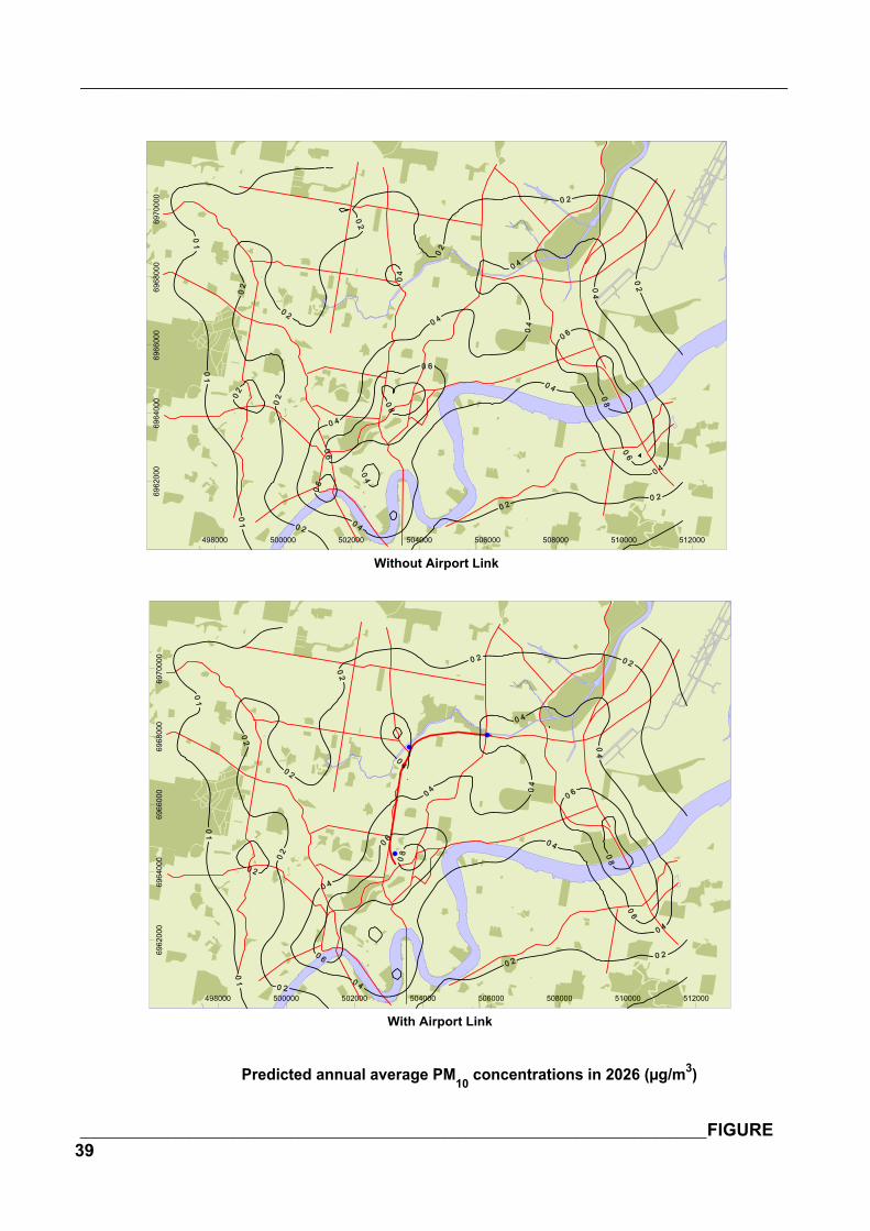
_______________________________________________________________________________
______________________________________________________________________________________FIGURE39
498000 500000 502000 504000 506000 508000 510000 512000
With Airport Link
6962
000
6964
000
6966
000
6968
000
6970
000
498000 500000 502000 504000 506000 508000 510000 512000
Without Airport Link
6962
000
6964
000
6966
000
6968
000
6970
000
Predicted annual average PM10 concentrations in 2026 (µg/m3)
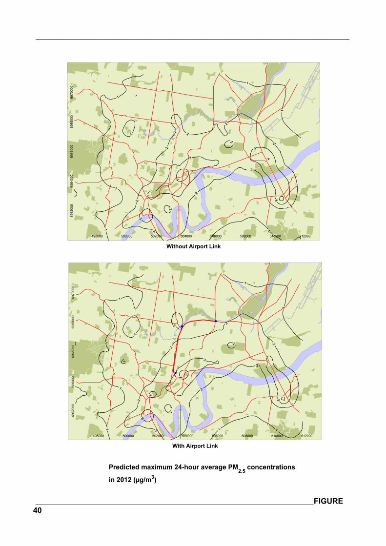
_______________________________________________________________________________
______________________________________________________________________________________FIGURE40
498000 500000 502000 504000 506000 508000 510000 512000
With Airport Link
6962
000
6964
000
6966
000
6968
000
6970
000
498000 500000 502000 504000 506000 508000 510000 512000
Without Airport Link
6962
000
6964
000
6966
000
6968
000
6970
000
Predicted maximum 24-hour average PM2.5 concentrations
in 2012 (µg/m3)
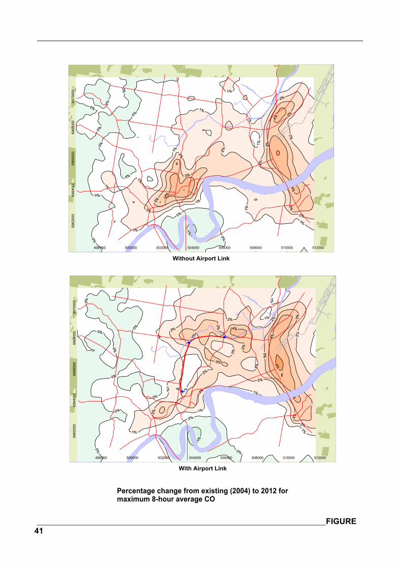
_______________________________________________________________________________
______________________________________________________________________________________FIGURE41
498000 500000 502000 504000 506000 508000 510000 512000
With Airport Link
6962
000
6964
000
6966
000
6968
000
6970
000
498000 500000 502000 504000 506000 508000 510000 512000
Without Airport Link
6962
000
6964
000
6966
000
6968
000
6970
000
Percentage change from existing (2004) to 2012 for maximum 8-hour average CO
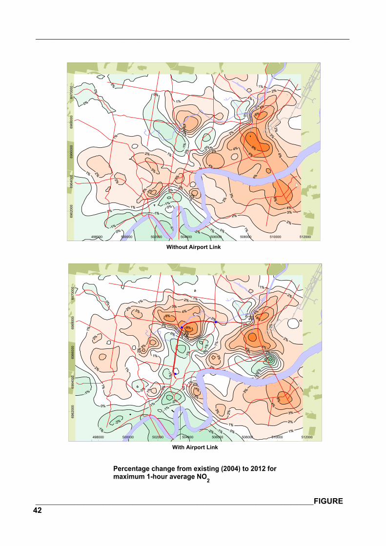
_______________________________________________________________________________
______________________________________________________________________________________FIGURE42
498000 500000 502000 504000 506000 508000 510000 512000
With Airport Link
6962
000
6964
000
6966
000
6968
000
6970
000
498000 500000 502000 504000 506000 508000 510000 512000
Without Airport Link
6962
000
6964
000
6966
000
6968
000
6970
000
Percentage change from existing (2004) to 2012 for maximum 1-hour average NO2
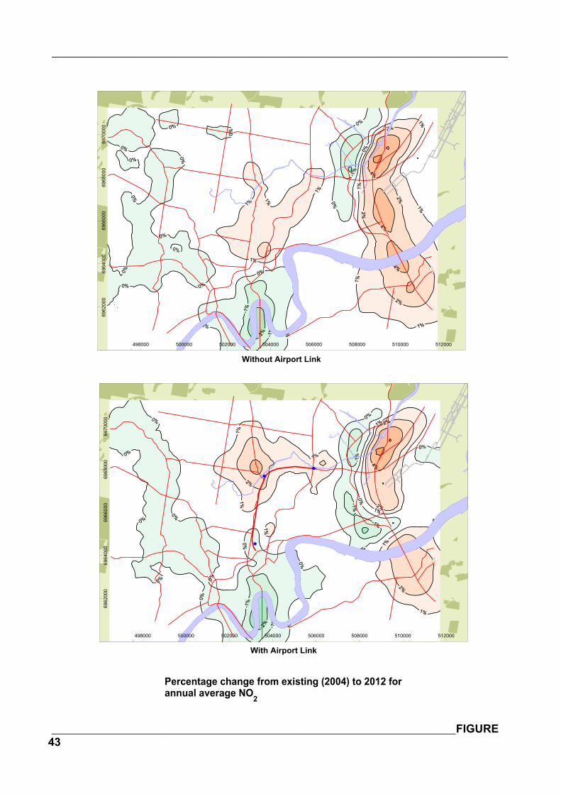
_______________________________________________________________________________
______________________________________________________________________________________FIGURE43
498000 500000 502000 504000 506000 508000 510000 512000
With Airport Link
6962
000
6964
000
6966
000
6968
000
6970
000
498000 500000 502000 504000 506000 508000 510000 512000
Without Airport Link
6962
000
6964
000
6966
000
6968
000
6970
000
Percentage change from existing (2004) to 2012 for annual average NO2
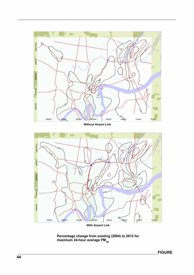
_______________________________________________________________________________
______________________________________________________________________________________FIGURE44
498000 500000 502000 504000 506000 508000 510000 512000
With Airport Link
6962
000
6964
000
6966
000
6968
000
6970
000
498000 500000 502000 504000 506000 508000 510000 512000
Without Airport Link
6962
000
6964
000
6966
000
6968
000
6970
000
Percentage change from existing (2004) to 2012 for maximum 24-hour average PM10
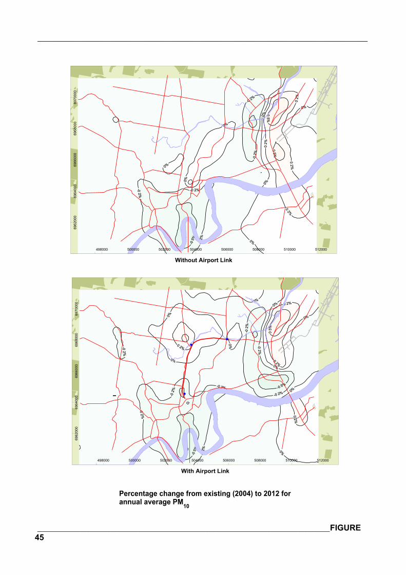
_______________________________________________________________________________
______________________________________________________________________________________FIGURE45
498000 500000 502000 504000 506000 508000 510000 512000
With Airport Link
6962
000
6964
000
6966
000
6968
000
6970
000
498000 500000 502000 504000 506000 508000 510000 512000
Without Airport Link
6962
000
6964
000
6966
000
6968
000
6970
000
Percentage change from existing (2004) to 2012 for annual average PM10
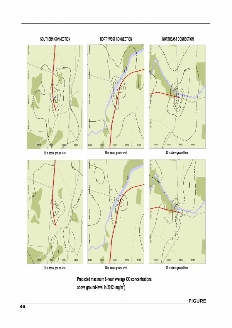
_______________________________________________________________________________
______________________________________________________________________________________FIGURE46
Predicted maximum 8-hour average CO concentrations above ground-level in 2012 (mg/m3)
505000 505500 506000 506500
50 m above ground level6
96
75
00
69
68
00
06
96
85
00
69
69
00
0
505000 505500 506000 506500
30 m above ground level
69675
00
69
680
00
6968
500
696
9000
502500 503000 503500 504000 504500
50 m above ground level
69
6700
0696
750
06
9680
00
6968
500
502500 503000 503500 504000 504500
30 m above ground level
69670
00
69
675
00
6968
000
696
8500
502500 503000 503500 504000
50 m above ground level
69
640
00
696450
06
9650
00
696
5500
502500 503000 503500 504000
30 m above ground level
6964
000
69645
00
6965
000
69
6550
0
SOUTHERN CONNECTION NORTHWEST CONNECTION NORTHEAST CONNECTION
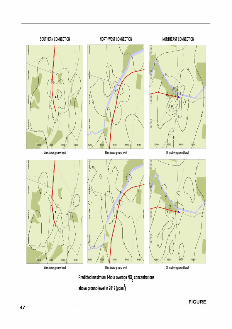
_______________________________________________________________________________
______________________________________________________________________________________FIGURE47
Predicted maximum 1-hour average NO2 concentrations
above ground-level in 2012 (µg/m3)
505000 505500 506000 506500
50 m above ground level6
96
75
00
69
68
00
06
96
85
00
696
90
00
505000 505500 506000 506500
30 m above ground level
69
67
50
06
96
80
00
69
68
50
06
96
90
00
502500 503000 503500 504000 504500
50 m above ground level
69
67
00
06
96
75
00
696
80
00
69
68
50
0
502500 503000 503500 504000 504500
30 m above ground level
69
67
00
06
96
75
00
69
68
00
06
96
85
00
502500 503000 503500 504000
50 m above ground level
69
64
00
06
96
45
00
696
50
00
69
65
50
0
502500 503000 503500 504000
30 m above ground level
69
64
00
06
96
45
00
69
65
000
69
65
50
0
SOUTHERN CONNECTION NORTHWEST CONNECTION NORTHEAST CONNECTION
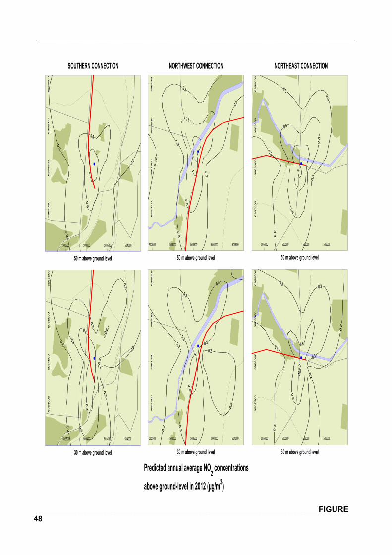
_______________________________________________________________________________
______________________________________________________________________________________FIGURE48
Predicted annual average NO2 concentrations
above ground-level in 2012 (µg/m3)
505000 505500 506000 506500
50 m above ground level6
96
75
00
69
68
00
06
96
85
00
69
69
00
0
505000 505500 506000 506500
30 m above ground level
69
67500
696
80
00
69685
00
696900
0
502500 503000 503500 504000 504500
50 m above ground level
69670
00
696750
06
968000
69
68500
502500 503000 503500 504000 504500
30 m above ground level
69
67000
696
75
00
69680
00
696850
0
502500 503000 503500 504000
50 m above ground level
696
40
00
696450
06
96500
06
965500
502500 503000 503500 504000
30 m above ground level
69
64000
69
64500
696
50
00
69655
00
SOUTHERN CONNECTION NORTHWEST CONNECTION NORTHEAST CONNECTION
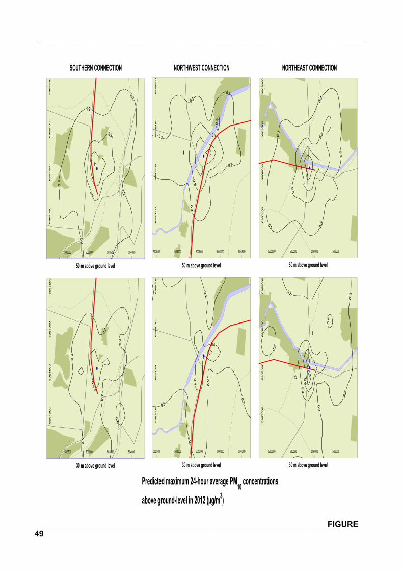
_______________________________________________________________________________
______________________________________________________________________________________FIGURE49
Predicted maximum 24-hour average PM10 concentrations
above ground-level in 2012 (µg/m3)
505000 505500 506000 506500
50 m above ground level6
96
75
00
69
68
00
06
96
85
00
69
69
00
0
505000 505500 506000 506500
30 m above ground level
69
67500
696
80
00
69685
00
696900
0
502500 503000 503500 504000 504500
50 m above ground level
69670
00
696750
06
968000
69
68500
502500 503000 503500 504000 504500
30 m above ground level
69
67000
696
75
00
69680
00
696850
0
502500 503000 503500 504000
50 m above ground level
696
40
00
696450
06
96500
06
965500
502500 503000 503500 504000
30 m above ground level
69
64000
69
64500
696
50
00
69655
00
SOUTHERN CONNECTION NORTHWEST CONNECTION NORTHEAST CONNECTION
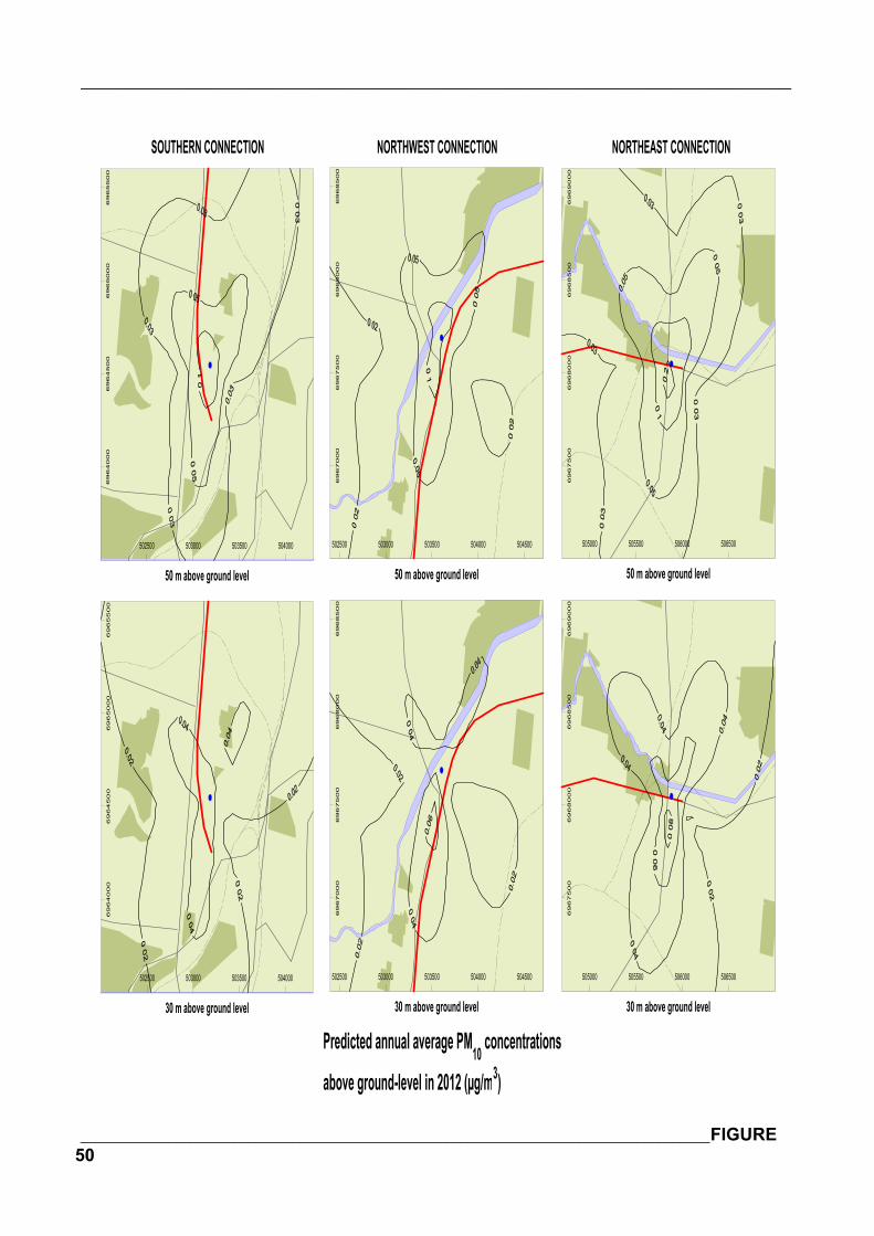
_______________________________________________________________________________
______________________________________________________________________________________FIGURE50
Predicted annual average PM10 concentrations
above ground-level in 2012 (µg/m3)
505000 505500 506000 506500
50 m above ground level6
96
75
00
69
68
00
06
96
85
00
69
69
00
0
505000 505500 506000 506500
30 m above ground level
69
67500
696
80
00
69685
00
696900
0
502500 503000 503500 504000 504500
50 m above ground level
69670
00
696750
06
968000
69
68500
502500 503000 503500 504000 504500
30 m above ground level
69
67000
696
75
00
69680
00
696850
0
502500 503000 503500 504000
50 m above ground level
696
40
00
696450
06
96500
06
965500
502500 503000 503500 504000
30 m above ground level
69
64000
69
64500
696
50
00
69655
00
SOUTHERN CONNECTION NORTHWEST CONNECTION NORTHEAST CONNECTION
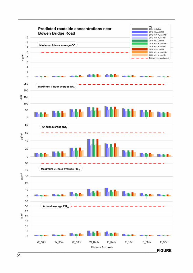
_______________________________________________________________________________
______________________________________________________________________________________FIGURE51
W_50m W_30m W_10m W_Kerb E_Kerb E_10m E_30m E_50m
Distance from kerb
0
5
10
15
20
25
30
35
g/m
3
Annual average PM10
0
10
20
30
40
50
g/m
3
Maximum 24-hour average PM10
0
20
40
60
80
g/m
3
Annual average NO2
0
50
100
150
200
250
g/m
3
Maximum 1-hour average NO2
0
2
4
6
8
10
12
14
16
mg/
m3
Maximum 8-hour average CO
Predicted roadside concentrations near Bowen Bridge Road
Key2004 (existing)2012 no AL or NB2012 with AL and NB2012 with AL no NB2016 no AL or NB2016 with AL and NB2016 with AL no NB2026 no AL or NB2026 with AL and NB2026 with AL no NBRelevant air quality goal
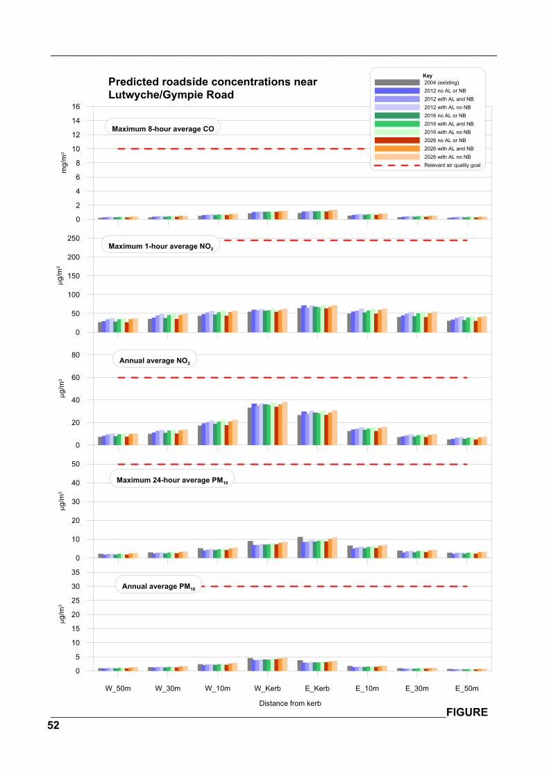
_______________________________________________________________________________
______________________________________________________________________________________FIGURE52
W_50m W_30m W_10m W_Kerb E_Kerb E_10m E_30m E_50m
Distance from kerb
0
5
10
15
20
25
30
35
g/m
3
Annual average PM10
0
10
20
30
40
50
g/m
3
Maximum 24-hour average PM10
0
20
40
60
80
g/m
3
Annual average NO2
0
50
100
150
200
250
g/m
3
Maximum 1-hour average NO2
0
2
4
6
8
10
12
14
16
mg/
m3
Maximum 8-hour average CO
Predicted roadside concentrations near Lutwyche/Gympie Road
Key2004 (existing)2012 no AL or NB2012 with AL and NB2012 with AL no NB2016 no AL or NB2016 with AL and NB2016 with AL no NB2026 no AL or NB2026 with AL and NB2026 with AL no NBRelevant air quality goal

_______________________________________________________________________________
______________________________________________________________________________________FIGURE53
W_50m W_30m W_10m W_Kerb E_Kerb E_10m E_30m E_50m
Distance from kerb
0
5
10
15
20
25
30
35
g/m
3
Annual average PM10
0
10
20
30
40
50
g/m
3
Maximum 24-hour average PM10
0
20
40
60
80
g/m
3
Annual average NO2
0
50
100
150
200
250
g/m
3
Maximum 1-hour average NO2
0
2
4
6
8
10
12
14
16
mg/
m3
Maximum 8-hour average CO
Predicted roadside concentrations near Gympie Road
Key2004 (existing)2012 no AL or NB2012 with AL and NB2012 with AL no NB2016 no AL or NB2016 with AL and NB2016 with AL no NB2026 no AL or NB2026 with AL and NB2026 with AL no NBRelevant air quality goal

_______________________________________________________________________________
______________________________________________________________________________________FIGURE54
W_50m W_30m W_10m W_Kerb E_Kerb E_10m E_30m E_50m
Distance from kerb
0
5
10
15
20
25
30
35
g/m
3
Annual average PM10
0
10
20
30
40
50
g/m
3
Maximum 24-hour average PM10
0
20
40
60
80
g/m
3
Annual average NO2
0
50
100
150
200
250
g/m
3
Maximum 1-hour average NO2
0
2
4
6
8
10
12
14
16
mg/
m3
Maximum 8-hour average CO
Predicted roadside concentrations near Sandgate Road south of East-West Arterial
Key2004 (existing)2012 no AL or NB2012 with AL and NB2012 with AL no NB2016 no AL or NB2016 with AL and NB2016 with AL no NB2026 no AL or NB2026 with AL and NB2026 with AL no NBRelevant air quality goal
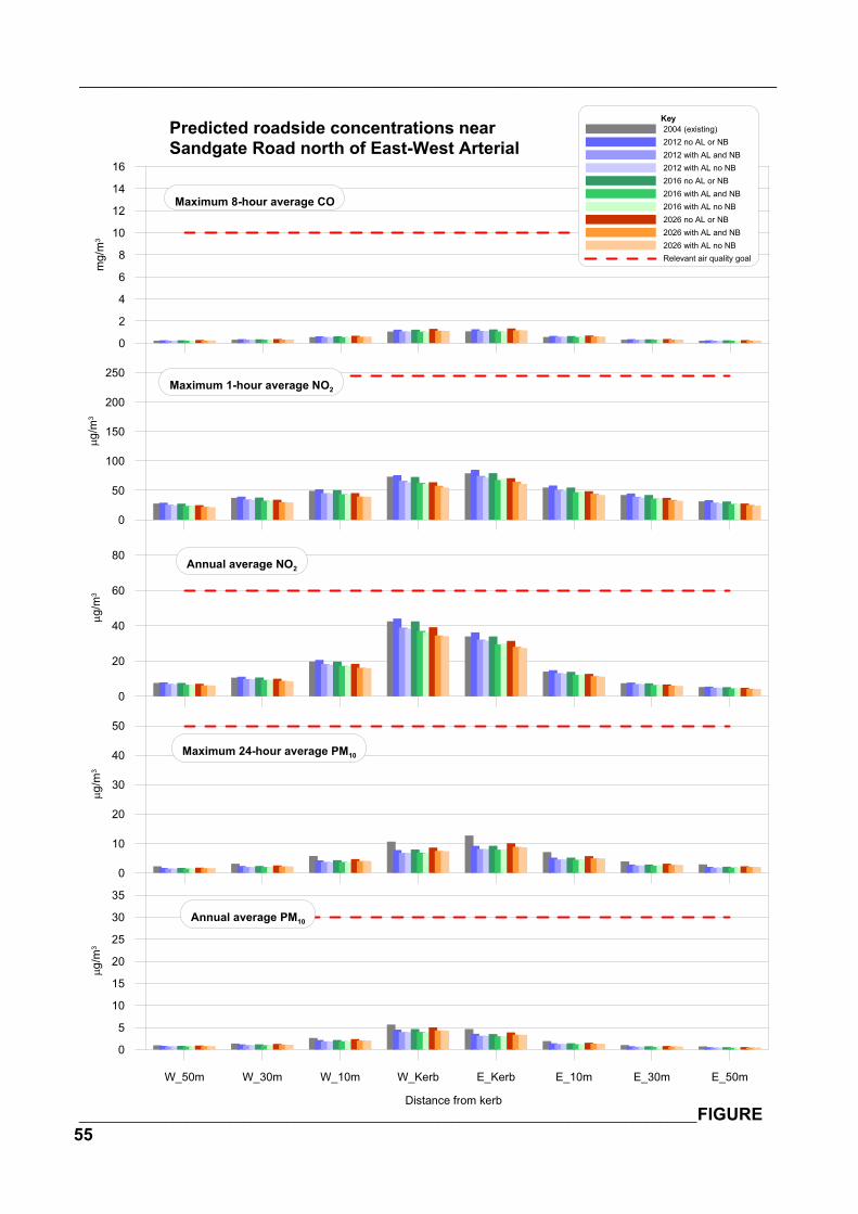
_______________________________________________________________________________
______________________________________________________________________________________FIGURE55
W_50m W_30m W_10m W_Kerb E_Kerb E_10m E_30m E_50m
Distance from kerb
0
5
10
15
20
25
30
35
g/m
3
Annual average PM10
0
10
20
30
40
50
g/m
3
Maximum 24-hour average PM10
0
20
40
60
80
g/m
3
Annual average NO2
0
50
100
150
200
250
g/m
3
Maximum 1-hour average NO2
0
2
4
6
8
10
12
14
16
mg/
m3
Maximum 8-hour average CO
Predicted roadside concentrations near Sandgate Road north of East-West Arterial
Key2004 (existing)2012 no AL or NB2012 with AL and NB2012 with AL no NB2016 no AL or NB2016 with AL and NB2016 with AL no NB2026 no AL or NB2026 with AL and NB2026 with AL no NBRelevant air quality goal
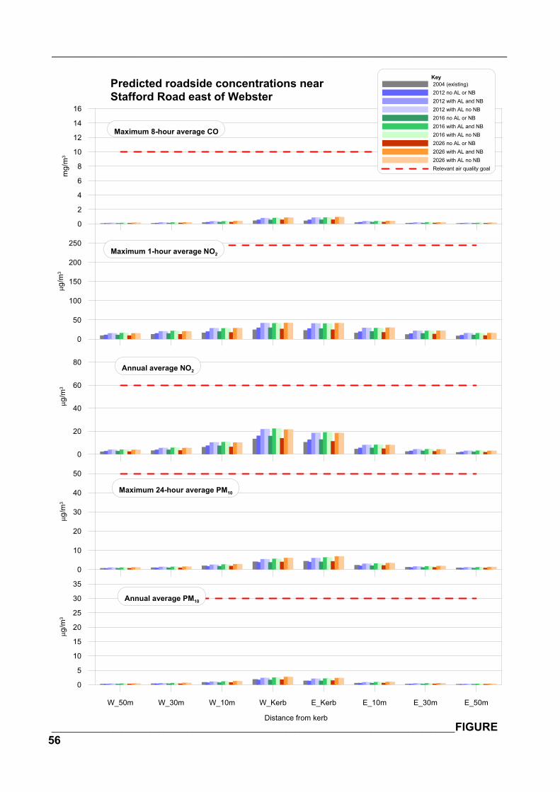
_______________________________________________________________________________
______________________________________________________________________________________FIGURE56
W_50m W_30m W_10m W_Kerb E_Kerb E_10m E_30m E_50m
Distance from kerb
0
5
10
15
20
25
30
35
g/m
3
Annual average PM10
0
10
20
30
40
50
g/m
3
Maximum 24-hour average PM10
0
20
40
60
80
g/m
3
Annual average NO2
0
50
100
150
200
250
g/m
3
Maximum 1-hour average NO2
0
2
4
6
8
10
12
14
16
mg/
m3
Maximum 8-hour average CO
Predicted roadside concentrations near Stafford Road east of Webster
Key2004 (existing)2012 no AL or NB2012 with AL and NB2012 with AL no NB2016 no AL or NB2016 with AL and NB2016 with AL no NB2026 no AL or NB2026 with AL and NB2026 with AL no NBRelevant air quality goal
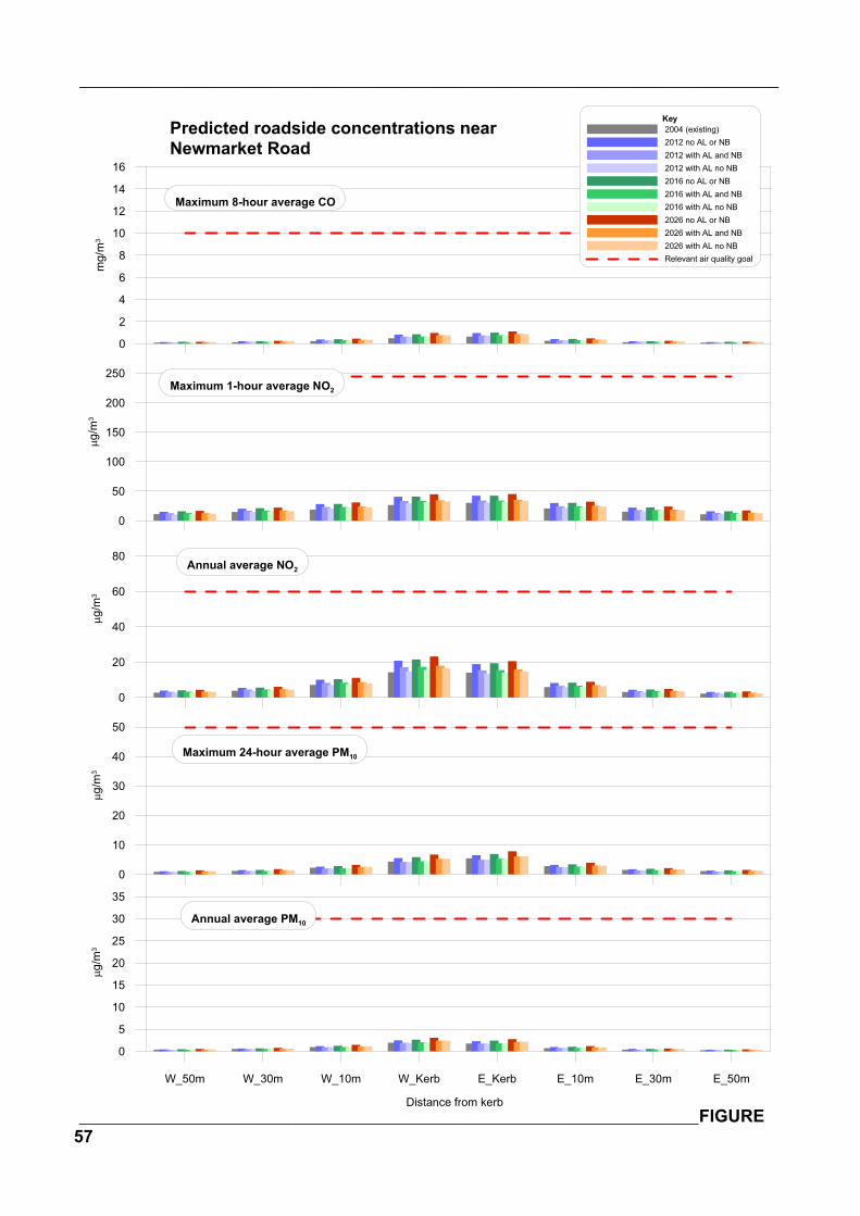
_______________________________________________________________________________
______________________________________________________________________________________FIGURE57
W_50m W_30m W_10m W_Kerb E_Kerb E_10m E_30m E_50m
Distance from kerb
0
5
10
15
20
25
30
35
g/m
3
Annual average PM10
0
10
20
30
40
50
g/m
3
Maximum 24-hour average PM10
0
20
40
60
80
g/m
3
Annual average NO2
0
50
100
150
200
250
g/m
3
Maximum 1-hour average NO2
0
2
4
6
8
10
12
14
16
mg/
m3
Maximum 8-hour average CO
Predicted roadside concentrations near Newmarket Road
Key2004 (existing)2012 no AL or NB2012 with AL and NB2012 with AL no NB2016 no AL or NB2016 with AL and NB2016 with AL no NB2026 no AL or NB2026 with AL and NB2026 with AL no NBRelevant air quality goal
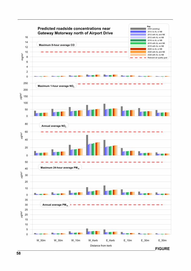
_______________________________________________________________________________
______________________________________________________________________________________FIGURE58
W_50m W_30m W_10m W_Kerb E_Kerb E_10m E_30m E_50m
Distance from kerb
0
5
10
15
20
25
30
35
g/m
3
Annual average PM10
0
10
20
30
40
50
g/m
3
Maximum 24-hour average PM10
0
20
40
60
80
g/m
3
Annual average NO2
0
50
100
150
200
250
g/m
3
Maximum 1-hour average NO2
0
2
4
6
8
10
12
14
16
mg/
m3
Maximum 8-hour average CO
Predicted roadside concentrations near Gateway Motorway north of Airport Drive
Key2004 (existing)2012 no AL or NB2012 with AL and NB2012 with AL no NB2016 no AL or NB2016 with AL and NB2016 with AL no NB2026 no AL or NB2026 with AL and NB2026 with AL no NBRelevant air quality goal
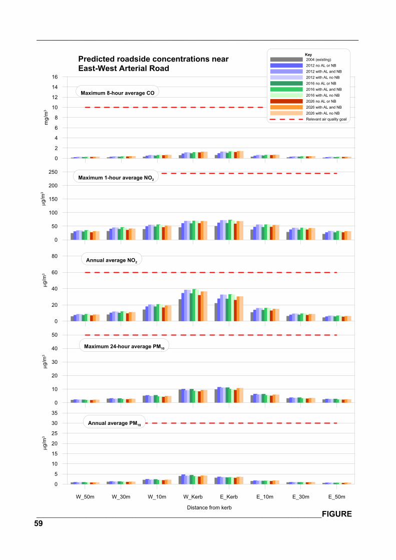
_______________________________________________________________________________
______________________________________________________________________________________FIGURE59
W_50m W_30m W_10m W_Kerb E_Kerb E_10m E_30m E_50m
Distance from kerb
0
5
10
15
20
25
30
35
g/m
3
Annual average PM10
0
10
20
30
40
50
g/m
3
Maximum 24-hour average PM10
0
20
40
60
80
g/m
3
Annual average NO2
0
50
100
150
200
250
g/m
3
Maximum 1-hour average NO2
0
2
4
6
8
10
12
14
16
mg/
m3
Maximum 8-hour average CO
Predicted roadside concentrations near East-West Arterial Road
Key2004 (existing)2012 no AL or NB2012 with AL and NB2012 with AL no NB2016 no AL or NB2016 with AL and NB2016 with AL no NB2026 no AL or NB2026 with AL and NB2026 with AL no NBRelevant air quality goal
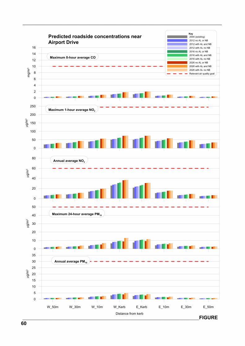
_______________________________________________________________________________
______________________________________________________________________________________FIGURE60
W_50m W_30m W_10m W_Kerb E_Kerb E_10m E_30m E_50m
Distance from kerb
0
5
10
15
20
25
30
35
g/m
3
Annual average PM10
0
10
20
30
40
50
g/m
3
Maximum 24-hour average PM10
0
20
40
60
80
g/m
3
Annual average NO2
0
50
100
150
200
250
g/m
3
Maximum 1-hour average NO2
0
2
4
6
8
10
12
14
16
mg/
m3
Maximum 8-hour average CO
Predicted roadside concentrations near Airport Drive
Key2004 (existing)2012 no AL or NB2012 with AL and NB2012 with AL no NB2016 no AL or NB2016 with AL and NB2016 with AL no NB2026 no AL or NB2026 with AL and NB2026 with AL no NBRelevant air quality goal
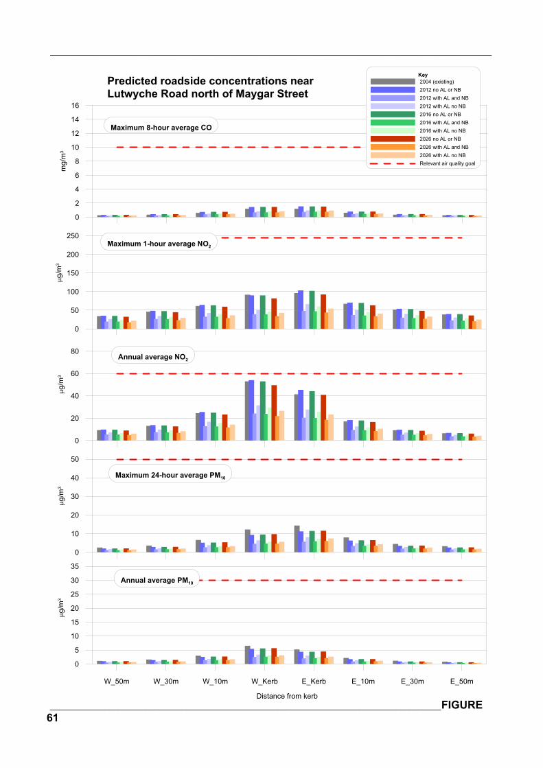
_______________________________________________________________________________
______________________________________________________________________________________FIGURE61
W_50m W_30m W_10m W_Kerb E_Kerb E_10m E_30m E_50m
Distance from kerb
0
5
10
15
20
25
30
35
g/m
3
Annual average PM10
0
10
20
30
40
50
g/m
3
Maximum 24-hour average PM10
0
20
40
60
80
g/m
3
Annual average NO2
0
50
100
150
200
250
g/m
3
Maximum 1-hour average NO2
0
2
4
6
8
10
12
14
16
mg/
m3
Maximum 8-hour average CO
Predicted roadside concentrations near Lutwyche Road north of Maygar Street
Key2004 (existing)2012 no AL or NB2012 with AL and NB2012 with AL no NB2016 no AL or NB2016 with AL and NB2016 with AL no NB2026 no AL or NB2026 with AL and NB2026 with AL no NBRelevant air quality goal
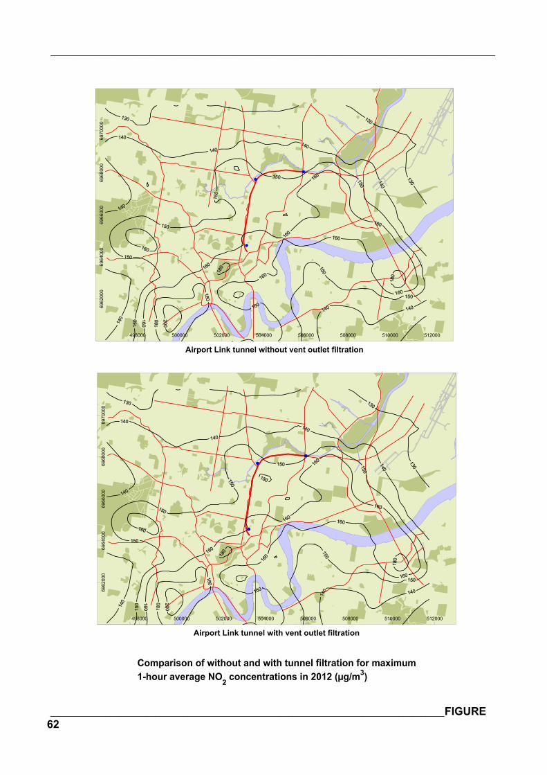
_______________________________________________________________________________
______________________________________________________________________________________FIGURE62
498000 500000 502000 504000 506000 508000 510000 512000
Airport Link tunnel with vent outlet filtration
6962
000
6964
000
6966
000
6968
000
6970
000
498000 500000 502000 504000 506000 508000 510000 512000
Airport Link tunnel without vent outlet filtration
6962
000
6964
000
6966
000
6968
000
6970
000
Comparison of without and with tunnel filtration for maximum 1-hour average NO2 concentrations in 2012 (µg/m3)
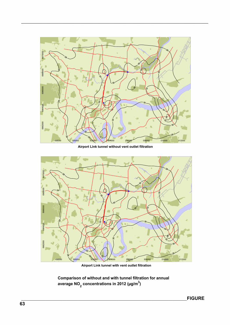
_______________________________________________________________________________
______________________________________________________________________________________FIGURE63
498000 500000 502000 504000 506000 508000 510000 512000
Airport Link tunnel with vent outlet filtration
6962
000
6964
000
6966
000
6968
000
6970
000
498000 500000 502000 504000 506000 508000 510000 512000
Airport Link tunnel without vent outlet filtration
6962
000
6964
000
6966
000
6968
000
6970
000
Comparison of without and with tunnel filtration for annualaverage NO2 concentrations in 2012 (µg/m3)
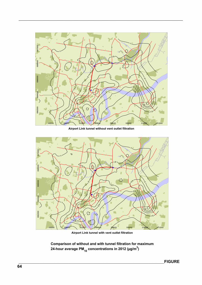
_______________________________________________________________________________
______________________________________________________________________________________FIGURE64
498000 500000 502000 504000 506000 508000 510000 512000
Airport Link tunnel with vent outlet filtration
6962
000
6964
000
6966
000
6968
000
6970
000
498000 500000 502000 504000 506000 508000 510000 512000
Airport Link tunnel without vent outlet filtration
6962
000
6964
000
6966
000
6968
000
6970
000
Comparison of without and with tunnel filtration for maximum24-hour average PM10 concentrations in 2012 (µg/m3)
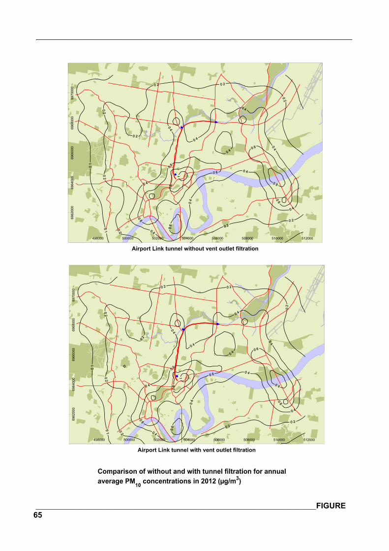
_______________________________________________________________________________
______________________________________________________________________________________FIGURE65
498000 500000 502000 504000 506000 508000 510000 512000
Airport Link tunnel with vent outlet filtration
6962
000
6964
000
6966
000
6968
000
6970
000
498000 500000 502000 504000 506000 508000 510000 512000
Airport Link tunnel without vent outlet filtration
6962
000
6964
000
6966
000
6968
000
6970
000
Comparison of without and with tunnel filtration for annualaverage PM10 concentrations in 2012 (µg/m3)
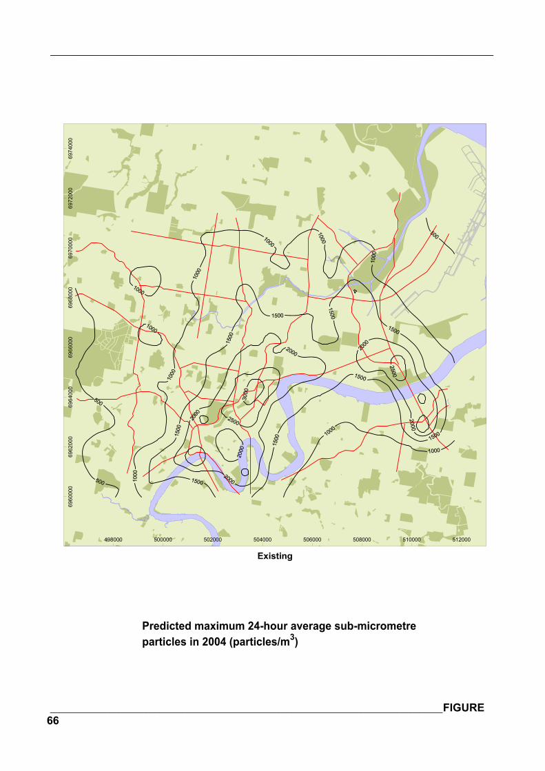
_______________________________________________________________________________
______________________________________________________________________________________FIGURE66
498000 500000 502000 504000 506000 508000 510000 512000
Existing
6960
000
6962
000
6964
000
6966
000
6968
000
6970
000
6972
000
6974
000
Predicted maximum 24-hour average sub-micrometreparticles in 2004 (particles/m3)
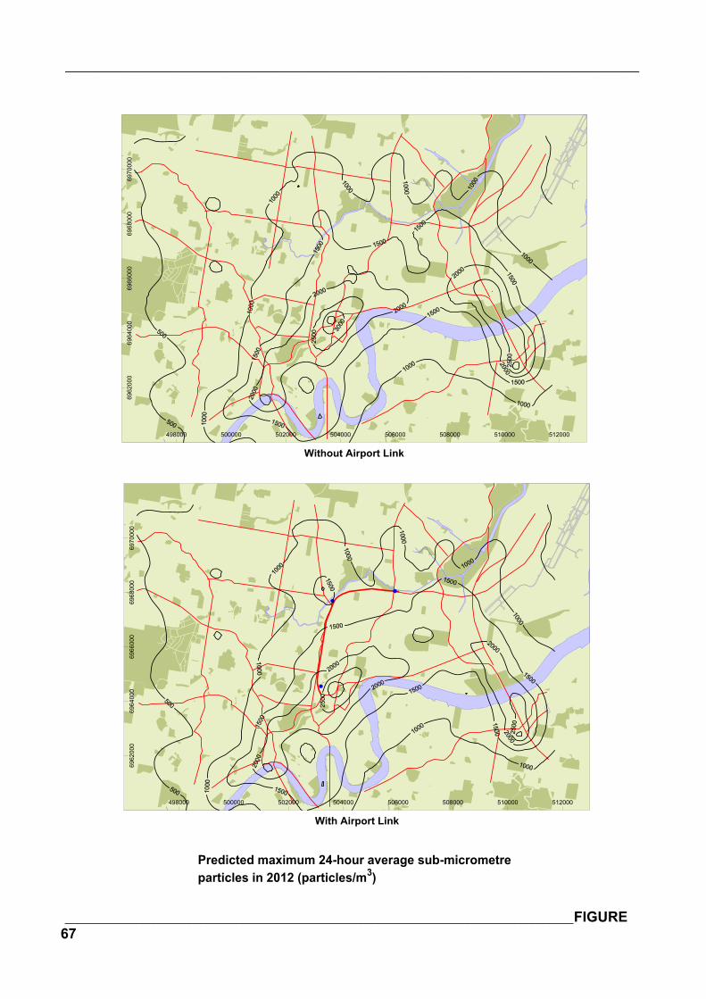
_______________________________________________________________________________
______________________________________________________________________________________FIGURE67
498000 500000 502000 504000 506000 508000 510000 512000
With Airport Link
6962
000
6964
000
6966
000
6968
000
6970
000
498000 500000 502000 504000 506000 508000 510000 512000
Without Airport Link
6962
000
6964
000
6966
000
6968
000
6970
000
Predicted maximum 24-hour average sub-micrometreparticles in 2012 (particles/m3)