AIR FORCE INSTITUTE OF TECHNOLOGY - dtic.mil effects of data replication on data exfiltration in mobile ad hoc networks utilizing reactive protocols thesis corey t. willinger, b.s.c.s

EFFECTS OF DATA REPLICATION ONDATA EXFILTRATION IN MOBILE AD HOC

NETWORKS UTILIZING REACTIVEPROTOCOLS

THESIS

Corey T. Willinger, Captain, USAF

AFIT-ENG-MS-15-M-035

DEPARTMENT OF THE AIR FORCEAIR UNIVERSITY

AIR FORCE INSTITUTE OF TECHNOLOGY

Wright-Patterson Air Force Base, Ohio

DISTRIBUTION STATEMENT AAPPROVED FOR PUBLIC RELEASE; DISTRIBUTION UNLIMITED.

The views expressed in this thesis are those of the author and do not reflect theofficial policy or position of the United States Air Force, Department of Defense,or the United States Government. This material is declared a work of the U.S.Government and is not subject to copyright protection in the United States.


EFFECTS OF DATA REPLICATION ON DATA EXFILTRATION IN MOBILE

AD HOC NETWORKS UTILIZING REACTIVE PROTOCOLS

THESIS

Presented to the Faculty

Department of Electrical and Computer Engineering

Graduate School of Engineering and Management

Air Force Institute of Technology

Air University

Air Education and Training Command

in Partial Fulfillment of the Requirements for the

Degree of Master of Science in Computer Science

Corey T. Willinger, B.S.C.S.

Captain, USAF

March 2015

DISTRIBUTION STATEMENT AAPPROVED FOR PUBLIC RELEASE; DISTRIBUTION UNLIMITED.




THESIS

Corey T. Willinger, B.S.C.S.Captain, USAF

Committee Membership:

Maj Brian G. Woolley (Chairman)

Dr. Douglas D. Hodson (Member)

Dr. David Jacques (Member)


Abstract

A swarm of autonomous unmanned aerial vehicles (UAVs) can provide a signifi-

cant amount of intelligence, surveillance, and reconnaissance (ISR) data where current

UAV assets may not be feasible or practical. As such, the availability of the data the

resides in the swarm is a topic that will benefit from further investigation. This thesis

examines the impact of file replication and swarm characteristics such as node mobil-

ity, swarm size, and churn rate on data availability utilizing reactive protocols. This

document examines the most prominent factors affecting the networking of nodes in

a mobile ad hoc network (MANET). Factors include network routing protocols and

peer-to-peer file protocols. It compares and contrasts several open source network

simulator environments. Experiment implementation is documented, covering design

considerations, assumptions, and software implementation, as well as detailing con-

stant, response and variable factors. Collected data is presented and the results show

that in swarms of sizes of 30, 45, and 60 nodes, file replication improves data avail-

ability until network saturation is reached, with the most significant benefit gained

after only one copy is made. Mobility, churn rate, and swarm density all influence

the replication impact.

iv

Acknowledgements

Above all else, I must recognize my wife’s unwavering support and dedication.

Her patience during the last eighteen months has been nothing short of heroic. To

my boys, for all the days and nights I spent holed up in the office, thank you and I’m

sorry you didn’t get much say in the matter.

I would like to thank my thesis advisor, for his guidance, knowledge, patience and

most of all, sense of humor. I would also like to thank my committee members, for

without their dedication to teaching, this wouldn’t have been possible.

Finally, I would like thank all the supervisors, mentors, and classmates that guided

and supported me over years.

Corey T. Willinger

v

Table of Contents

Page

Abstract . . . . . . . . . . . . . . . . . . . . . . . . . . . . . . . . . . . . . . . . . . . . . . . . . . . . . . . . . . . . . . . iv

Acknowledgements . . . . . . . . . . . . . . . . . . . . . . . . . . . . . . . . . . . . . . . . . . . . . . . . . . . . . . . v

List of Figures . . . . . . . . . . . . . . . . . . . . . . . . . . . . . . . . . . . . . . . . . . . . . . . . . . . . . . . . . . ix

List of Tables . . . . . . . . . . . . . . . . . . . . . . . . . . . . . . . . . . . . . . . . . . . . . . . . . . . . . . . . . . . xi

List of Acronyms . . . . . . . . . . . . . . . . . . . . . . . . . . . . . . . . . . . . . . . . . . . . . . . . . . . . . . . xii

I. Introduction . . . . . . . . . . . . . . . . . . . . . . . . . . . . . . . . . . . . . . . . . . . . . . . . . . . . . . . . 1

1.1 Research Objective . . . . . . . . . . . . . . . . . . . . . . . . . . . . . . . . . . . . . . . . . . . . . . 21.2 Document Structure . . . . . . . . . . . . . . . . . . . . . . . . . . . . . . . . . . . . . . . . . . . . . 3

II. Related Work . . . . . . . . . . . . . . . . . . . . . . . . . . . . . . . . . . . . . . . . . . . . . . . . . . . . . . . 4

2.1 MANETs / VANETs / FANETs . . . . . . . . . . . . . . . . . . . . . . . . . . . . . . . . . . 42.2 Physical Layer . . . . . . . . . . . . . . . . . . . . . . . . . . . . . . . . . . . . . . . . . . . . . . . . . . 52.3 Routing Protocols . . . . . . . . . . . . . . . . . . . . . . . . . . . . . . . . . . . . . . . . . . . . . . . 6

2.3.1 Proactive Protocols . . . . . . . . . . . . . . . . . . . . . . . . . . . . . . . . . . . . . . . . 72.3.2 Reactive Protocols . . . . . . . . . . . . . . . . . . . . . . . . . . . . . . . . . . . . . . . . 102.3.3 Hybrid Protocols . . . . . . . . . . . . . . . . . . . . . . . . . . . . . . . . . . . . . . . . . 192.3.4 Virtual Backbones . . . . . . . . . . . . . . . . . . . . . . . . . . . . . . . . . . . . . . . . 222.3.5 Quality of Service . . . . . . . . . . . . . . . . . . . . . . . . . . . . . . . . . . . . . . . . 232.3.6 Analysis of differences in routing protocols . . . . . . . . . . . . . . . . . . . 25

2.4 Peer-to-Peer File Systems . . . . . . . . . . . . . . . . . . . . . . . . . . . . . . . . . . . . . . . 272.4.1 Distributed Hash Tables . . . . . . . . . . . . . . . . . . . . . . . . . . . . . . . . . . . 28

2.5 Combining peer-to-peer (P2P) and MANETs. . . . . . . . . . . . . . . . . . . . . . . 342.5.1 Integration Paradigms . . . . . . . . . . . . . . . . . . . . . . . . . . . . . . . . . . . . 342.5.2 Optimized Routing Independent Overlay

Network (ORION) . . . . . . . . . . . . . . . . . . . . . . . . . . . . . . . . . . . . . . . . 382.5.3 ORION+ . . . . . . . . . . . . . . . . . . . . . . . . . . . . . . . . . . . . . . . . . . . . . . . . 412.5.4 Mobile Peer-to-Peer (MPP) protocol . . . . . . . . . . . . . . . . . . . . . . . . 422.5.5 Availability Schemes . . . . . . . . . . . . . . . . . . . . . . . . . . . . . . . . . . . . . . 42

2.6 Simulation Environments . . . . . . . . . . . . . . . . . . . . . . . . . . . . . . . . . . . . . . . . 442.6.1 Network Simulator Version 2/3 . . . . . . . . . . . . . . . . . . . . . . . . . . . . . 452.6.2 OMNeT++ . . . . . . . . . . . . . . . . . . . . . . . . . . . . . . . . . . . . . . . . . . . . . . 452.6.3 Comparison of Performance . . . . . . . . . . . . . . . . . . . . . . . . . . . . . . . . 46

2.7 Summary . . . . . . . . . . . . . . . . . . . . . . . . . . . . . . . . . . . . . . . . . . . . . . . . . . . . . 47

vi

Page

III. Methodology . . . . . . . . . . . . . . . . . . . . . . . . . . . . . . . . . . . . . . . . . . . . . . . . . . . . . . 49

3.1 Experimental Design . . . . . . . . . . . . . . . . . . . . . . . . . . . . . . . . . . . . . . . . . . . . 503.1.1 Apparatus . . . . . . . . . . . . . . . . . . . . . . . . . . . . . . . . . . . . . . . . . . . . . . . 513.1.2 Simulation Design . . . . . . . . . . . . . . . . . . . . . . . . . . . . . . . . . . . . . . . . 52

3.2 Assumptions . . . . . . . . . . . . . . . . . . . . . . . . . . . . . . . . . . . . . . . . . . . . . . . . . . . 543.2.1 Response Variables . . . . . . . . . . . . . . . . . . . . . . . . . . . . . . . . . . . . . . . 543.2.2 Independent Variables . . . . . . . . . . . . . . . . . . . . . . . . . . . . . . . . . . . . . 553.2.3 Control Factors . . . . . . . . . . . . . . . . . . . . . . . . . . . . . . . . . . . . . . . . . . 563.2.4 Data Collection and Reduction . . . . . . . . . . . . . . . . . . . . . . . . . . . . . 58

3.3 Summary . . . . . . . . . . . . . . . . . . . . . . . . . . . . . . . . . . . . . . . . . . . . . . . . . . . . . 58

IV. Results and Analysis . . . . . . . . . . . . . . . . . . . . . . . . . . . . . . . . . . . . . . . . . . . . . . . . 61

4.1 Aggregate Values . . . . . . . . . . . . . . . . . . . . . . . . . . . . . . . . . . . . . . . . . . . . . . . 614.1.1 Query Success Rate . . . . . . . . . . . . . . . . . . . . . . . . . . . . . . . . . . . . . . . 624.1.2 Transfer Success Rate . . . . . . . . . . . . . . . . . . . . . . . . . . . . . . . . . . . . . 624.1.3 Query Time . . . . . . . . . . . . . . . . . . . . . . . . . . . . . . . . . . . . . . . . . . . . . 644.1.4 Transfer Time . . . . . . . . . . . . . . . . . . . . . . . . . . . . . . . . . . . . . . . . . . . 64

4.2 Results by Node Count . . . . . . . . . . . . . . . . . . . . . . . . . . . . . . . . . . . . . . . . . . 654.2.1 Query Success Rate . . . . . . . . . . . . . . . . . . . . . . . . . . . . . . . . . . . . . . . 654.2.2 Transfer Success Rate . . . . . . . . . . . . . . . . . . . . . . . . . . . . . . . . . . . . . 674.2.3 Query Time . . . . . . . . . . . . . . . . . . . . . . . . . . . . . . . . . . . . . . . . . . . . . 674.2.4 Transfer Time and Hop Count . . . . . . . . . . . . . . . . . . . . . . . . . . . . . 684.2.5 Total System Packets . . . . . . . . . . . . . . . . . . . . . . . . . . . . . . . . . . . . . 68

4.3 Results by Mobility . . . . . . . . . . . . . . . . . . . . . . . . . . . . . . . . . . . . . . . . . . . . . 694.3.1 Transfer Success Rate . . . . . . . . . . . . . . . . . . . . . . . . . . . . . . . . . . . . . 714.3.2 Query and Transfer Time . . . . . . . . . . . . . . . . . . . . . . . . . . . . . . . . . . 714.3.3 Hop Count . . . . . . . . . . . . . . . . . . . . . . . . . . . . . . . . . . . . . . . . . . . . . . 72

4.4 Results by Churn . . . . . . . . . . . . . . . . . . . . . . . . . . . . . . . . . . . . . . . . . . . . . . . 744.4.1 Query Success Rate . . . . . . . . . . . . . . . . . . . . . . . . . . . . . . . . . . . . . . . 754.4.2 Transfer Success Rate . . . . . . . . . . . . . . . . . . . . . . . . . . . . . . . . . . . . . 754.4.3 Query Time . . . . . . . . . . . . . . . . . . . . . . . . . . . . . . . . . . . . . . . . . . . . . 774.4.4 Transfer Time and Hop Count . . . . . . . . . . . . . . . . . . . . . . . . . . . . . 77

4.5 Availability by Time . . . . . . . . . . . . . . . . . . . . . . . . . . . . . . . . . . . . . . . . . . . . 784.5.1 Grouped by Nodes . . . . . . . . . . . . . . . . . . . . . . . . . . . . . . . . . . . . . . . . 794.5.2 Grouped by Speed . . . . . . . . . . . . . . . . . . . . . . . . . . . . . . . . . . . . . . . . 814.5.3 Grouped by Churn . . . . . . . . . . . . . . . . . . . . . . . . . . . . . . . . . . . . . . . 81

4.6 Summary . . . . . . . . . . . . . . . . . . . . . . . . . . . . . . . . . . . . . . . . . . . . . . . . . . . . . 85

V. Conclusions and Recommendations for Future Work . . . . . . . . . . . . . . . . . . . . 86

5.1 Conclusions . . . . . . . . . . . . . . . . . . . . . . . . . . . . . . . . . . . . . . . . . . . . . . . . . . . . 865.2 Future Work . . . . . . . . . . . . . . . . . . . . . . . . . . . . . . . . . . . . . . . . . . . . . . . . . . . 87

vii

Page

Bibliography . . . . . . . . . . . . . . . . . . . . . . . . . . . . . . . . . . . . . . . . . . . . . . . . . . . . . . . . . . . 89

viii

List of Figures

Figure Page

1 Model of topology of wireless ad hoc network byunit-disk graphs . . . . . . . . . . . . . . . . . . . . . . . . . . . . . . . . . . . . . . . . . . . . . . . . . 6

2 Illustration of MPR selection . . . . . . . . . . . . . . . . . . . . . . . . . . . . . . . . . . . . . 10

3 Forward and reverse path formation in AODV . . . . . . . . . . . . . . . . . . . . . . 15

4 Channel selection in CA-AODV . . . . . . . . . . . . . . . . . . . . . . . . . . . . . . . . . . 17

5 AntHocNet Multi-Path Selection . . . . . . . . . . . . . . . . . . . . . . . . . . . . . . . . . . 21

6 Distributed Hash Table Lookup Process . . . . . . . . . . . . . . . . . . . . . . . . . . . 29

7 Content Addressable Network Grid . . . . . . . . . . . . . . . . . . . . . . . . . . . . . . . . 33

8 MANET File System Implementations . . . . . . . . . . . . . . . . . . . . . . . . . . . . . 37

9 ORION Query Broadcast . . . . . . . . . . . . . . . . . . . . . . . . . . . . . . . . . . . . . . . . 39

10 ORION Query Response . . . . . . . . . . . . . . . . . . . . . . . . . . . . . . . . . . . . . . . . . 40

11 Query/Transfer Success Rates and Mean Time (AllNodes) . . . . . . . . . . . . . . . . . . . . . . . . . . . . . . . . . . . . . . . . . . . . . . . . . . . . . . . 63

12 Query/Transfer Success Rates and Mean Time by Nodes . . . . . . . . . . . . 66

13 Mean Hop Count and Transfer Time by Node Count . . . . . . . . . . . . . . . . 69

14 Mean Total Sum of Applicaiton Level Packets . . . . . . . . . . . . . . . . . . . . . . 70

15 Query/Transfer Success Rates and Mean Time by Speed . . . . . . . . . . . . . 73

16 Mean Hop Count and Transfer Time by Speed . . . . . . . . . . . . . . . . . . . . . . 74

17 Query/Transfer Success Rates and Mean Time by Churn . . . . . . . . . . . . . 76

18 Mean Hop Count and Transfer Time by Churn . . . . . . . . . . . . . . . . . . . . . 78

19 Mean Transfer Success Rate by Time, Replication, andNodes . . . . . . . . . . . . . . . . . . . . . . . . . . . . . . . . . . . . . . . . . . . . . . . . . . . . . . . . . 80

20 Mean Transfer Success Rate by Time, Replication, andSpeed . . . . . . . . . . . . . . . . . . . . . . . . . . . . . . . . . . . . . . . . . . . . . . . . . . . . . . . . . 82

ix

Figure Page

21 Mean Transfer Success Rate by Time, Replication, andChurn . . . . . . . . . . . . . . . . . . . . . . . . . . . . . . . . . . . . . . . . . . . . . . . . . . . . . . . . . 84

x

List of Tables

Table Page

1 Routing Protocol Feature Comparison . . . . . . . . . . . . . . . . . . . . . . . . . . . . . 27

2 Response Variable Summary . . . . . . . . . . . . . . . . . . . . . . . . . . . . . . . . . . . . . 59

3 Independent Variable Summary . . . . . . . . . . . . . . . . . . . . . . . . . . . . . . . . . . . 59

4 Constant Factors Summary . . . . . . . . . . . . . . . . . . . . . . . . . . . . . . . . . . . . . . 60

5 ANOVA for Query Success . . . . . . . . . . . . . . . . . . . . . . . . . . . . . . . . . . . . . . . 66

6 ANOVA for Transfer Success . . . . . . . . . . . . . . . . . . . . . . . . . . . . . . . . . . . . . 68

xi

List of Acronyms

Acronym Definition

ARA Ant-Colony-Based Routing Algorithm

ACO Ant Colony Optimization

AODV Ad hoc On-demand Distance Vector

CA-AODV Channel Assignment AODV

CAN Content Addressable Network

CDS connected dominating set

DHT distributed hash table

DSDV Destination-Sequenced Distance-Vector

DSR Dynamic Source Routing

EC erasure coding

ISR intelligence, surveillance, and reconnaissance

FANET flying ad hoc network

FEC forward error correction

MAC media access control

MANET mobile ad hoc network

MCDS minimally connected dominating set

MPR multi-point relay

xii

NPDU network protocol data unit

OLSR Optimized Link State Routing

ORION Optimized Routing Independent Overlay Network

OSI Open Systems Interconnect

P2P peer-to-peer

QoS quality of service

RREP route reply

RREQ route request

UAV unmanned aerial vehicle

VANET vehicular ad hoc network

VoIP Voice over Internet Protocol

VRR Virtual Ring Routing

xiii



I. Introduction

With UAVs becoming smaller, lighter, and easier to replace, the study of UAV

swarms has gained momentum as an area of academic study. In military areas of

research, UAV swarms have been popularized for their robustness, i.e. their ability to

loose members and reform to continue operation. This redundancy provides a graceful

degradation to the overall capabilities of the system. In the context of ISR missions,

not only are the assets key to mission objectives, but more importantly, so is the

data that the individual assets collect. How this information is stored and extracted

from the swarm network is an area of critical on-going research. This thesis argues

that file replication can increase data survivability in a system where the amount of

data generated exceeds the capability to ex-filtrate the data, but extent of the benefit

provided by file replication is limited by characteristics of the UAV swarm. Extensive

work has been done in the last decade regarding various routing protocols in mobile ad

hoc networks (MANETs), much of which stems from the seminal work of Perkins and

Bhagwat[39]. Recent research has applied these concepts to collections of UAVs due

to inherently mobile nature. Peer-to-peer (P2P) file sharing applications have also

has been covered extensively, looking at traditional peer-to-peer transfer protocols

such as Ding and Bhargavas work in Peer-to-peer File-Sharing over Mobile Ad Hoc

Networks [21], or even MANET specific applications such as Klemm’s Optimized

Routing Independent Overlay Network (ORION) [32]. Despite over a decade’s worth

of research, little information exists specifically on the resiliency of data in a MANET

1

P2P file system hosted by a UAV swarm where the goal is to maintain data until

it can be requested. Furthermore, since the flight-time of each UAV is limited, a

UAV rotation schedule must be enforced where UAVs enter and leave the system

to maintain 24 hour operations. Additionally, some UAVs may suffer mechanical

failures, unexpected operating parameters (e.g. weather, temp, etc.), or in the case of

military applications, destruction from opposing forces. These factors induce churn

or attrition that must factor in to the swarm’s operation. Such a scenario exists where

individual autonomous UAVs can form a robust MANET but lack a high-bandwidth

connection back to a central control facility. Additionally, the UAV swarm itself

may maintain the data on separate nodes as part of distributed artificial intelligence

system, where instead of extracting the data, the system needs to maintain copies

for its own use. These scenarios have applications to the military, disaster recovery

operations, geological survey and others.

The complexity of MANET operation, compared to that of a traditional, fixed

infrastructure network creates an abundance of factors to examine. Such factors in-

clude overhead from network routing and file system control, which impact bandwidth

available for data extraction. Additional factors such as replication rate, replication

strategy, file size, and number of nodes in the system all impact performance.

1.1 Research Objective

The objective of this work is to analyze the impact of data replication on availabil-

ity and response times in a reactive peer-to-peer file system running on an airborne

MANET. The experimental domain is a network simulator, wherein factors such as

replication levels, number of nodes in the system, mobility (airspeed), and churn rate

(attrition) can be varied to observe their effects on the system. The hope is that the

results will shed light on the optimal configurations for future implementations. The

2

insight here is that increasing replication will lead to an increase in availability, but

only until the overhead cost of the replication (in network bandwidth) exceeds the

capacity of the ad hoc network. Furthermore, results indicate that adjusting node

mobility and swarm size play a critical part in data availability.

1.2 Document Structure

The remainder of this thesis is organized as follows: Chapter II covers basic

MANET principles, P2P file system principles, and an overview of current network

simulators. Chapter III details the methodology used in conducting the experiments

and enumerates the simulation parameters, (e.g. response variables, control variables,

constant factors). Finally, Chapter IV presents the results of the experiments, while

Chapter V draws conclusions and gives recommendations for potential future work.

3

II. Related Work

This chapter provides necessary background on ad hoc networks. In particu-

lar, it provides, a broad overview of ad hoc networks followed by a discussion of

the differences between various applications of ad hoc networks in mobile ad hoc

networks (MANETs), vehicular ad hoc networks (VANETs), and flying ad hoc net-

works (FANETs). Much of the research into ad hoc networks revolves around the

different algorithms and protocols utilized for implementation. These protocols can

be segregated into two primary camps, proactive and reactive. Proactive protocols

act similar to traditional routing protocols where network maps are built ahead of

time and reactive protocols build routing tables only on an as-needed basis. In ad-

dition, topics on the usage of virtual backbones, quality of service, and cross-layer

optimization are also covered as they relate to potential future work.

Built on such proactive and reactive protocols for ad hoc networks are applica-

tions, one which is the focus of this thesis is the implementation of a peer-to-peer

network file system that supports file/data replication, along with the challenges that

are presented by ad hoc network implementations that do not exist in traditional

infrastructure networks.

Finally, the chapter closes with a look at the current state of modeling ad hoc

networks, the various simulators used, as well as a survey of simulation versus an

actual network performance.

2.1 MANETs / VANETs / FANETs

MANET research was popularized in the late 1990’s and has continued unabated

since. Research involving ad hoc networks can be categorized three different ways,

with respect to the mobility of the devices that are connected. Traditionally, the term

4

MANET relates to any type of node that is mobile in a 2D or 3D space. Typically,

this is representative of personal computing devices such as cell phones, tablets, or

other personal data assistants. A VANET refers to a network typically embedded in

motor vehicles and presents a unique study landscape due to mobility constraints of

traffic patterns. Boukerche et al. [11] also refers to this is as V2V routing. FANETs

are identical to VANETs with the exception that the focus is on the application of

ad hoc networks for airborne systems. Each category possess unique challenges, thus

making distinctions critical. This thesis will focus primarily on FANETs, but will use

the term MANET to generalize all mobile ad hoc networks, unless noted otherwise.

For simplification, connections are modeled using the unit-disk graph (UDG)

paradigm; that is each network will be represented as a disk with a radius that

is equal to the range of the radio used for transmission. However, this could be

expanded to take into consideration links of various weights such as frequency, band-

width, distance, etc. We will also assume a homogeneous grouping of nodes; every

node is of the same class and subject to the same constraints. Figure 1, inspired by

the work of Wan et al. [53] provides an excellent visual of a unit-disk representation.

Additional figures will use this figure as a baseline for continuity.

2.2 Physical Layer

A variety of wireless protocols have been selected for use in the study of MANETs.

Most prominently has been the standard IEEE 802.11 protocols (Wifi), specifically

the a, b, g, and n variations. The 802.11 specification supports transmission speeds

from 2 - 600 MBs/sec with ranges up to 250 meters [26]. The IEEE 802.15 speci-

fication for wireless networking, better known as Bluetooth (802.15.1), is extremely

useful for short range communication. It supports transfer rates from 1 to 24 MB/sec,

depending on the version of the protocol used. The 802.15.4 specification introduces

5

Figure 1. Model of topology of wireless ad hoc network by unit-disk graphs - Inspiredby Wan et al. [53], this illustration shows each node as a solid circle labeled with a letter, and itscorresponding radio range denoted by the dashed circle.

low-power specifications which may prove to be extremely useful when applied to a

system of ultra small unmanned aerial vehicles (UAVs) flying in a tight cluster. Bhag-

wat and Segall [10] highlight the differences between design paradigms for Bluetooth

networks, known as scatternets, and traditional MANETs.

2.3 Routing Protocols

Research involving MANETs has led to an abundance of various routing protocols.

This section will presents prominent protocols and closely examines those that relate

directly to this thesis. Perkins and Bhagwat [39] state that the challenge of routing

in an ad hoc network boils down to a distributed shortest path problem, and the

only primary difference between protocols is how the routing table is constructed and

what information is maintained. Boukerche et al. [11] gives a survey of over 115 dif-

ferent routing protocols for MANETs. Here protocols are divided into nine different

6

categories based on the following design paradigms: Source-initiated (Reactive and

on-demand), Table-driven or Pro-active, Hybrid, Geographical, Hierarchical, Multi-

cast, Geographical Multicast and Power-Aware. While this categorization covers the

gamut, most papers simply limit the grouping to Proactive and Reactive types.

The routing protocol chosen for a particular application can have a dramatic

effect on overall system performance. Factors to take into account include: network

size, fault tolerance, delay tolerance, mobility rate, system-knowledge (how much

information does each node possess on the state of the network), node-density, and

others.

According to Boukerche et al. [11], next-hop routing methods can be categorized

into two groups, link-state and distance-vector. With Link-State, nodes maintain

network topology with the cost of each link. Periodic network broadcasts update

all other nodes with new information and the receiving nodes apply a shortest path

algorithm to determine next hops for each destination. However, with Distance-

Vector, each node maintains a list of distances to each destination for each neighbor.

The neighbor with the smallest distance to the destination is used as the next hop. To

maintain table freshness, nodes periodically broadcast their links to their neighbors.

2.3.1 Proactive Protocols.

Proactive protocols attempt to maintain an up-to-date picture of the network by

updating their routing tables before they are needed. For as static network, this

type of routing protocol works well and is typified by standard infrastructure routing

protocols like the Routing Information Protocol. However, in a dynamic network

environment where nodes are changing connections at varying rates, this type of

proactive routing scheme can prove problematic. Two prominent proactive protocols,

7

Destination-Sequenced Distance-Vector (DSDV) and Optimized Link State Routing

(OLSR) are detailed below.

2.3.1.1 Destination-Sequenced Distance-Vector.

Perkins and Bhagwat [39] chose to use a distance-vector method as an ad hoc net-

work routing protocol because, as they stated, “Compared to the link-state method, it

is computationally more efficient, easier to implement and requires much less storage

space.”

Under DSDV routing, packets are transmitted to their neighbors either via media

access control (MAC) address or network address. Each node maintains a routing

table entry for every destination and the number of hops required to reach it. Ad-

ditionally, a sequence number is associated with each entry that corresponds to the

last known sequence number of the destination node. This sequence number is used

to identify freshness of route information and is similar in function to that of a Lam-

port Clock [34]. Open Systems Interconnect (OSI) layer 2 and 3 addresses are also

included in the broadcast packet.

Perkins and Bhagwat describe two different types of broadcast packets for route

updates. The first, an incremental update, should be crafted to fit inside one net-

work protocol data unit (NPDU). The second is a “full dump”, which might require

multiple NPDUs [39]. The full dump broadcasts can be used when the size of the

incremental packets reach the NPDU size.

While DSDV implemented a distance-vector methodology for route propagation,

OLSR leverages link-state to create its routing tables.

8

2.3.1.2 Optimized Link State Routing.

The protocol, developed by Jacquet and Muhlethaler [28], starts with each node

broadcasting “HELLO” messages to its neighbors (i.e. nodes that it has a direct

link with). Each hello message lists the node’s neighbors and their corresponding

link-state. This provides a mechanism for each node to be aware of all one-hop and

two-hop neighbors. From these neighbors, each node calculates a set of multi-point

relays (MPRs). Each node selected as a MPR must meet two critical conditions.

First, the node must possess a bi-directional link, and second, the set of MPRs is

such that it covers all two-hop neighbors. Obviously, with fewer nodes, optimality

increases. This is illustrated in Figure 2.

The MPRs are used to decrease the amount of control traffic generated when

propagating topology changes across the network. This is similar to the virtual back-

bone discussed later in the chapter, however it is calculated at each node as a local

optimization, rather than a system wide distributed algorithm. Changes in topology

are disseminated through topology control messages. These messages are broadcast

to all neighbor nodes, but only MPRs forward the control message. Using these

control messages, each node builds a complete routing table for each node in the

network. Jacquet elaborates on the route calculation algorithm and provides a proof

of correctness for optimality.

It is important to understand proactive protocols and to understand the benefits

that reactive protocols offer in MANETs. This section provided a brief description

of two prominent protocols, DSDV and OLSR. The following section provide insight

into reactive protocols.

9

Figure 2. Illustration of MPR selection - Node F represents an arbitrary node in the systemwith 1 hop connections represented by a solid line. Two-hop connections from Node F ar representedby dashed lines. A locally optimized MPR selection is shown as gray nodes.

2.3.2 Reactive Protocols.

Reactive protocols differ from proactive protocols in that routes are only generated

“on-demand”, i.e. they only update routing information when a route does not exist,

or is too old. This type of protocol has the benefit of cutting down on the number of

control packets in the MANET, particularly in MANETs with high mobility, at the

expense of potential delays in route acquisition. The following section will focus on Ad

hoc On-demand Distance Vector (AODV), AODV variants, as well as Dynamic Source

Routing (DSR). AODV is covered in-depth due to the implementation of Optimized

Routing Independent Overlay Network (ORION), a peer-to-peer file transfer protocol

that is discussed later in the chapter.

2.3.2.1 Ad hoc On-Demand Distance Vector.

AODV is a widely popular routing protocol. It was first proposed by Charles E.

Perkins and Elizabeth M. Royer, in 1999 in their paper, “Ad hoc On-Demand Distance

10

Vector Routing”, with substantial assistance from Pravin Bhagwat [40]. The AODV

routing protocol will be covered in-depth since it forms the foundation upon which

the experiments were conducted for the current research. According to Perkins, the

genesis of research into networks based on mobile nodes began with DARPA research

involving packet radio networks. AODV is based on DSDV, as explained earlier, but

overcomes the limitations on network size imposed by the O(n2) growth of control

messages required to keep every node’s routing table current. As such, Perkins’

motivation was to “minimize broadcasts and transmission latency” [40].

2.3.2.1.1 Implementation. A critical component of the AODV protocol

is the concept that routes are not maintained for nodes that do not exist on an

active path. Perkins refers to this as “pure on-demand route acquisition” [40]. Next,

nodes are made aware of nodes in its local neighborhood by means of a periodic

hello message. This hello message is basically a ping to all nodes that are within the

transmit range (1 hop) of the source node and is not forwarded to any node beyond the

receiver. The combination of hello messages and on-demand route acquisition creates

a system of two different management requirements, one for local connectivity, and

one for general topology, such as when the node is participating in an active request

for a route or active file transfer.

2.3.2.1.2 Route Discovery. AODV makes use of the DSR broadcast rou-

tine (explained in a later section), with a slight alteration. Instead of propagating

information about routing to the source node, each intermediary node only updates

information about it neighbors. As Perkins explains, this reduction in overhead has

a dramatic effect as the size of the network increases, thus making AODV more scal-

able [40].

11

The route, or path, discovery algorithm begins when a node does not currently

have a route to a requested node in its route table. To begin, the node broadcasts a

packet, known as a route request (RREQ), to its immediate neighbors. Each RREQ

contains the source-addr (network address of node requesting route), source-sequence-

num (counter that is incremented with each message), broadcast-id (counter that is

incremented with each new RREQ), dest-addr (network address of node that the

source is attempting to reach), dest-seq-num (last known sequence number of desti-

nation), and the hop-cnt (number of hops packet has taken).

When a neighbor node receives the RREQ, it can respond in one of three ways.

First, if it has already seen the RREQ (the pairing of source address and broadcast id

creates a unique key to identify), it will drop the packet and take no action. Passing

that conditional, if it has a route to the destination, it can reply to the source with a

route reply (RREP). Finally, if it does not have a route, it increments the packet hop

count and re-broadcasts the RREQ to its’ neighbors. If the node re-broadcasts the

RREQ, it logs the request with the dest-addr, source-addr, broadcast-id, the exp-time

(time until request expires), and the source-sequence-num.

This information has two purposes. The first is to drop future requests with the

same id. This is critical to ensure RREQ loops are not formed. In addition to this,

the information is necessary to set up the return path.

2.3.2.1.3 Reverse Path. The sequence number of the source is used to

keep entries up-to-date. If a node receives a new RREQ with a higher sequence

number, it updates its route entries with the address of the node that it first received

the RREQ from. The expiration time out is set to a value that allows enough time

for the reply to come back. While Perkins and Royer don’t cover it explicitly, this

parameter should be tuned to allow enough time for the reply to come back from

the destination. Setting this value too high will lead to unnecessary look-ups to a

12

factor of O(n2), where n is the number of nodes in the system (although most realistic

scenarios would not pass through every node). The net result of these RREQ forwards

is that once the final destination is reached, the route back to the source has already

been constructed. This can be visualized in Figure 3a.

2.3.2.1.4 Forward Path. Once the RREQ reaches a node that possess

a route to the destination node, the node checks to see if the destination sequence

number of the RREQ is higher than the destination sequence number stored locally.

If it is, the node assumes that its route is stale, clears its entry, and proceeds with

the RREQ re-broadcast. If its destination sequence number is greater than or equal

to that of the RREQ, a path has been established and the process now proceeds with

returning the information to the original source node as represented in Figure 3a. To

accomplish this, the node with a route to the destination node replies to its neighbor

from which it received the RREQ with a new RREP packet. The RREP packet

contains the Destination address, Source address, Destination Sequence Number, Hop

Count, and Lifetime (i.e., how long the route will stay active).

This RREP packet is forwarded along the reverse path that has already been

created, with each node setting up a reverse pointer to the node that it received

the RREP packet from (updating its route table). Since the node that received the

RREP packet has new information, it updates the activity timers on the routes to

keep them from being deleted. This process continues until the RREP packet reaches

the source node. As the node receives additional RREP packets, it will update its

route table if two conditions are met. First, if the destination-sequence number for

the destination node is higher than that which is currently stored, or second, if the

node receives a RREP with the same destination sequence number and a lower hop

count. This algorithm works to improve the route while the information is being

passed back to the source. Just like the RREQ packets, if it has a lower sequence

13

number, the packet is dropped to reduce unnecessary traffic. Once the RREP packet

arrives at the original source destination, the route is complete and the source node

can begin communication with the destination node as seen in Figure 3b.

2.3.2.1.5 Route Maintenance. When there is a break in an active route,

detected by either a lack of a “hello” message, or a link-layer acknowledgment

(LLACKS ) failure, action must be taken to update nodes on the path to the source

that the route is no longer tenable. This is done through sending an RREP packet

with an incremented sequence number and a hop count set to ∞ [40].

While Perkins does not cover this topic at length in his paper, the fact that the

route table only contains entries for a short duration provides an interesting area

of study. This duration, or activity timeout is a tuned parameter that needs to be

adjusted to ensure optimal performance. Expected node mobility and network traffic

should be evaluated to help determine appropriate values. As node mobility increases,

the frequency of link-layer failures increases (assuming non-static mobility pattern).

A link-failure message is sent back to the source node where it will initiate a new

RREQ, again flooding the system. If the network is active, valid route entries will be

refreshed often, limiting the scope of the RREQ flood.

2.3.2.2 Ad hoc On-demand Distance Vector Variants.

Several papers introduce variations on AODV in attempts to increase the pro-

tocol’s utility in various situations. The following paragraphs cover a few of the

significant AODV based protocols.

2.3.2.2.1 Channel Assignment Ad hoc On-demand Distance Vector

Routing. Gong and Midkiff [22] assert that since the 802.11 protocol doesn’t work

well in a multi-hop wireless environment (based on the work of Xu and Saadawi),

14

(a) Reverse Path Formation

(b) Forward Path Formation

Figure 3. Forward and reverse path formation in AODV - The reverse path is constructedin figure 3a. RREQ packets (solid line) are broadcast at each node if it has not yet seen the RREQand it does not have a valid route to the requested node. If a node contains a valid route, itsends a RREP along the reverse path, establishing a forward path. Figure 3b shows the completedcommunication channel with the destination node.

15

a method for handling channel selection is required to reduce interference between

neighboring nodes. Unfortunately, as Gong points out, it is not possible to eliminate

all interference since the distributed channel assignment problem is NP -complete.

Channel Assignment AODV (CA-AODV) mirrors AODV with the exception that it

carries additional information in the RREQ and RREP packets to support multiple

channels. At each hop, if a neighbor node has been already assigned a channel, a

new one is randomly selected. During the RREP, if a channel is already in use at

the next hop (due to an already existing route), the next node along the RREP (1

hop closer to the source) is informed and it selects a new channel for the route being

established. Figure 4 can help aid in the understanding of this processes; you can see

that node A already has a route to node M, utilizing node I on Channel 2. Node D is

requesting a route to node N that passes through node I. Since node G does not have

an active route to node N, it randomly assigns one of its available channels (in this

case, 2) to the route. The RREQ proceeds to its destination, node N then initiates

the RREP process as in AODV. Node I, aware that it currently is using channel 2,

informs node G through the RREP packet to choose a different channel. When node

G receives the packet, it chooses a new available channel (in this case, for the route.

It is important to note that changing of the selected channel is only important during

the RREP, as the RREQ packet is flooded, and many nodes will not be part of the

forward route.

2.3.2.2.2 Ad hoc On-Demand Multipath Distance Vector Routing.

Zapata [58] present a variant to the traditional AODV routing protocol that calcu-

lates multiple disjoint and loop free paths as part of the initial route creation phase.

The author’s reasoning for this process is sound. The largest drawback to reactive

protocols is the network traffic generated during a flood request to establish a new

16

Figure 4. Channel selection in CA-AODV - An active route exists between nodes A and M.Node D requests a route to node N on channel 2 as well. Node I informs node G to select a differentavailable channel during the RREP process to de-conflict the channel assignment.

route. With a multi-path algorithm, a new route request only has to be performed

when all current established routes fail, thus reducing the number of flooded RREQs.

2.3.2.2.3 Ant-Colony-Based Routing Algorithm. Ant-Colony-Based

Routing Algorithm (ARA) is an extension of the AODV protocol, but implements

components of Ant Colony Optimization (ACO) algorithms. For the unaware, an

ACO algorithm uses “pheromone” trails to find an optimal solution to a given problem

using multiple agents. Over time, these multiple agents converge on an optimal

solution. This is achieved by the ant agents depositing a set amount of pheromone

on the edges selected for use in route to the destination and again on the way back.

This pheromone evaporates at a set rate so that paths that aren’t taken will decrease

in pheromone levels, and paths that are utilized will be reinforced and its pheromone

levels will increase, thus increasing the future likeliness of selection.

In the case of ARA routing, specially crafted packets are the “ants” and each node

updates the packets, as well as certain local variables based on the status of these

17

ant packets. The length of the path that the ACO algorithm is optimizing in this

case is hop-count, however, it can be extended to any other applicable metric, such

as capacity, congestion, power, or combinations thereof. Caro refers to two different

types of ants, FANTs and BANTs which are analogous to the RREQ and RREP

packets of AODV [15]. A key departure is that these packets are routed based on

pheromone levels of neighbor nodes, with some stochastic randomization included to

increase breadth of the search space and not get trapped in a localized optimization.

Once a FANT reaches its destination, it reinforces nodes along the reverse path headed

to the source with additional pheromones. This makes these nodes more likely to be

selected as intermediaries for future packets. Link failures are handled in a similar way

to AODV. Route Error messages are generated if a node doesn’t receive confirmation

that the next hop received the packet. It sets the pheromone level for the failed node

to 0 and sends Route Error message to the previous node to process. This chain is

continued until the Route Error message reaches the source node, at which time it

will generate a new request for a route.

2.3.2.3 Dynamic Source Routing.

DSR, developed by Maltz, Broch, and Johnson, was designed to have very low

overhead to support high mobility and is very similar to AODV with few excep-

tions [29]. The primary difference is that it maintains multiple routes for each desti-

nation. When a RREQ is forwarded, the intermediate node appends its IP address

to the packet. When the packet reaches the destination, it replies along the route,

including the list of all the addresses that the packet went through [2]. As Ade states,

maintenance of the route is performed through confirmations that the packet was re-

ceived either at the link or network layer. If the source detects a broken link, it can

either use a different cached route or request a new route. The other difference is that

18

the protocol uses source routing instead of the routes from the intermediate node. In

their initial design, [29] make the assumption that all radios operate in promiscuous

mode; that is every packet is delivered to the network layer, regardless of the MAC

layer addressing. This allows nodes to “overhear” packets destined for them even if

they are addressed to another node in the route before them in a process known as

“Automatic Route Shortening” [29]. This also allows the node to update its routing

table with information from the packet, even though it is not part of the active route.

2.3.3 Hybrid Protocols.

Research has also looked at combining proactive and reactive protocols into a

hybrid approach. While these protocols tend to increase the complexity of implemen-

tation, they hope to exploit advanced algorithm techniques to achieve more efficient

routing mechanisms. Two examples of hybrid protocols are AntHocNet, which is a

specific protocol and virtual backbones, which describes a class of hybrid protocols.

2.3.3.1 AntHocNet.

AntHocNet was introduced by [15], which “combines reactive route setup with

proactive route probing, maintenance and improvement”. It uses a multi-path algo-

rithm based on principles of standard ACO algorithms such as ARA. The AntHocNet

protocol begins with a reactive route setup phase. During this phase, forward ants

dubbed “reactive forward ants” are broadcast towards a destination and ”backward

ants” are returned as in other ACO protocols. AntHocNet then departs from other

ACO algorithms through the use of ”proactive forward ants” that are used to mon-

itor and improve current routes while data is being transmitted. Instead of sending

Route Error messages back to the source in the event of a link failure, as in ARA,

19

AntHocNet attempts to perform local repair or warn earlier nodes in the path of the

problem. Caro calculates route selection probability Pnd as

Pnd =(T ind)

β1

Σj∈N id(T ijd)

β1, β1 ≥ 1 (1)

where T ind is the pheromone value (quality of solution) of reaching node d from node i

through node n. N id represents the set of neighbors of i to which a path to d is known.

Caro uses β1 as a tuning parameter that can be leveraged to adjust the exploratory

behavior of the ants. Each ant is marked as F sd (k), where k is the replica number of

the same ant initiated from source node s with destination d. If F sd reaches a node

with no entries for node d, it will broadcast F sd to all neighbors, otherwise, it will

unicast F sd to nodes in its route table for node d.

During the course of route formation, if a node receives multiple ants of the

same generation (think same broadcast-id and sequence number from AODV), it will

compare the ants current hop count and travel time and forward it on if it is within a

certain acceptance factor of the best ant recorded of that generation. This supports

both multi-path routing and limiting control traffic by discarding ants following bad

routes. As Caro points out, the problem with this policy by itself is the formation of

kite-shape paths due to the automatic acceptance of the first ant to reach the node.

This is seen by the thick lines in Figure 5 where node E is requesting a path to node

G. To correct for this kite behavior, an additional tuning parameter is evaluated that

takes into account the first node selected from the source, with preference given to

paths that take different routes. This aides in the building of uniquely disjoint paths

to improve route selection options in the event of a link failure, as illustrated by the

dashed lines in Figure 5. These paths, while less optimal, improve resiliency.

Once the forward ant reaches the destination node, the reverse ant is sent back

to perform further pheromone updates. The amount of pheromone added is based

20

Figure 5. AntHocNet Multi-Path Selection - Solid lines indicate typical ant pathing behavior.Dashed lines are the result of adding an additional tuning parameter to favor disjoint points at nodeswith a low hop count.

on the estimated time to reach the destination node, and a system-wide average

estimation of the time to complete one hop. According to Caro, the use of a system-

wide constant instead of a local calculation prevents route oscillation due to changing

local conditions such as congestion and channel access activities [15].

Once a route has been established, data packets can be sent to the destination

nodes. This is done in a similar fashion to the forward ants. Since each node maintains

multiple routes for each node, each hop is again selected stochastically where

Pnd =(T ind)

β2

Σj∈N id(T ijd)

β2, β2 ≥ β1 (2)

The key difference is that a higher exponent is utilized to perform a more greedy

selection in regards to better paths [15]. With proactive ants being utilized, this

21

process has the effect of automatic load balancing as congested nodes will decrease

in pheromone levels with respect to equally feasible neighbors.

2.3.4 Virtual Backbones.

Virtual backbones present an opportunity to reduce the amount of control traffic

necessary to operate an ad hoc network. Of particular note is Das’s use of a minimally

connected dominating set (CDS) as a virtual backbone to function as a back-up

route for packets, and as well as the primary means to compute and update routes

for packets, i.e. its a control subgraph [20]. However, some protocols such as DSR

and AODV dynamically calculate routes on an as needed basis, and as such, virtual

backbones have less utility. None-the-less, it was a topic of active research in the

ad hoc community network for over a decade, with the most recent research focus

centered around evolutionary algorithms such as Ant Colony Optimization [35, 38, 53].

The formation of a virtual backbone is grounded in the graph theory concept of

dominated sets. As such, Wan et al. describe a dominated set as follows:

Given a graph G = (V,E), a dominating set V ′ ⊂ V such that each node in V −V ′

is adjacent to some node in V ′, with a connected dominating set being a DS which

also induces a connected sub graph [53].

While the construction of a CDS can be done in polynomial time, finding a min-

imally connected dominating set (MCDS) is known to be NP-Hard. Furthermore,

since we are dealing with a dynamic environment, an approximation algorithm that

finds a MCDS quickly is preferred as enumerating all possible solutions is not feasible

based on the time constraints of the problem domain O(2n). Further complicating

the problem is the distributed nature of the nodes, which imparts a latency delay for

any communication between nodes.

22

Much research has been done in the area of MCDS problems. Butenko looks at

the MCDS problem from a different stand-point in which nodes attempt to remove

themselves from the CDS (pruning) using a modified leader election algorithm [13],

while others look at the problem from a centralized/decentralized standpoint [24, 5,

53].

Algorithm 1 illustrates an Ant Colony Optimization implementation of a virtual

backbone. This algorithm is based of the work of Jovanovic and Tuba [30] and was

utilized in coursework complementary to this thesis to build a prototype simulator

using the Unity3D engine.

2.3.5 Quality of Service.

All of the routing algorithms presented thus far fail to recognize the importance of

quality of service (QoS) for multimedia applications such as video streaming and Voice

over Internet Protocol (VoIP) communication. If a UAV swarm has video capability

or is supporting another system that does, it is reasonable to assume that there may

be a requirement to establish a live feed through the swarm back to some centralized

location. Furthermore, while obvious that our UAVs do not have pilots, the potential

exists for the swarm to act as a relay for VoIP communication from other sources.

While this thesis is not taking QoS into consideration, it has been a central theme to

a number of research papers generated over the last decade [8, 16, 36, 31, 48].

Tanenbaum and Van Steen [50] lists a number of factors that must be considered

when discussing QoS in the general sense. These factors include, required bit rate,

session set-up delay, end-to-end delay, jitter (delay variance), and round-trip delay.

While buffering is a useful technique for handling QoS with video applications, it

is not appropriate for services that require packets to arrive in the correct sequence

with the correct timing (such as VoIP transmissions). As Tanenbaum and Van Steen

23

Algorithm 1: ACO Based Psuedo Code

Initialize source node = j0;while time allows (delay termination) do

foreach ant i dowhile CDS is incompleted (|VOut > 0) (feasibility) do

Step 2: poll list of neighbors (next state generator)foreach neighbor(j) = k do

if k /∈ EdgeList thenincrement nodeCounter;add k to edgelist

select node k ∈ EdgeList: based on(weight) (selection) ;if rand > weight then

exploit:select ni with MAX τi · degreeki ;

elseexplore:

select ni with probabilityτj ·degreekj∑

i∈EdgeListkτjdegreeki

;

Reinforcement: Local Level;move to next node: j ← k ;update message counter;update return route matrix with pointer to node nj−1;

forward result to supervisor;if Best solution then

while not at j0 doupdate Global level τj;

Reinforcement: (dependent on specific optimization goal)Evaporation: (dependent on node mobility)

j ← nj−1 (based on route matrix);

Output: Best solution found(solution);

24

[50, 162] point out, the use of forward error correction (FEC) can assist with this.

FEC entails encoding extra information in each packet so that if packets are lost in

route, they can be reconstructed using the other packets. FEC is also used in the

form of erasure coding (EC) in distributed file management systems such as Tahoe-

LAFS as part of its replication scheme. Altman and De Pellegrini [4] examine the

impact of FEC and Fountain Codes in a Delay Tolerant ad hoc Network. While FEC

and EC concepts relate to routing, they are better discussed in the context of file

management, and thus outside the scope of this section. Bagwari et al. [7] evaluate

the impact of additional nodes in an AODV network and its impact on QoS and

concluded that increasing the number of nodes from 45 to 60 increases the overall

QoS of the network as measured in packets received, packets dropped, and overall

network load.

2.3.6 Analysis of differences in routing protocols.

Now that a number of protocols and concepts have been examined, comparisons

between protocols can help show how the routing algorithms impact the performance

of the system. Of course, as protocols have been developed over the last one and half

decades, a number of papers have been published documenting such comparisons [2,

15, 25, 46].

While not providing any data for analysis, Ade and Tijare [2] provides a useful

comparison of features regarding the predominant protocols - DSDV, DSR, AODV,

and OLSR. This comparison of traits is summarized in Table 1.

Sharma [46] compares the performance of AODV, DSR, and AntHocNet and

concluded that AntHocNet suffers in cases of high mobility and small node buffer

sizes. The paper states that the proactive use of ants induces large overhead delay

and reducing the number of proactive ants reduces the quality of route information.

25

Restricting ant usage to purely reactive behavior eliminates control overhead, but

doesn’t result in significant gains over AODV and DSR.

Gunes et al. [25] compared ARA to AODV, DSR, and DSDV, evaluating several

different factors against changing pause durations. While this information is useful for

UAV swarms that have hover capability such as quad-copters, it could be extended to

UAVs without hover capability flying in tight orbits over a geographic area where their

orbits do not change the topology. Obviously, in the later scenario, the data link layer

would require longer range capability than what is provided by 802.11. Additional

research would need to be conducted of course, since the simulation results can not be

extended beyond the hardware technology simulated. None-the-less, Gunes finds that

as Pause Time increases from 100 to 900 seconds, the protocols perform in the follow-

ing descending order based on delivery rate: DSR, ARA, AODV, DSDV. However,

as Pause Time reaches 900 seconds, all protocols perform universally well [25].

Caro analyzes the performance of AntHocNet with respect to its father, AODV,

in regards to both node speed and pause time [15] using the Qualnet simulation

framework. The data shows that AntHocNet outperforms AODV by roughly 5% at

10 m/s and increases this performance by 2% as node mobility increases to 50 m/s.

Over the same mobility space, the data shows that AntHocNet reduces the mean end-

to-end packet delay by 10-20 ms. When node pause time is considered, AntHocNet

has a 5 - 7% advantage in packet delivery ratio, but this advantage quickly tapers

off as node pause time increases past 240 seconds. In the simulation set-up, Caro

explains that they intentionally used a sparse network to highlight the strengths of the

AntHocNet approach where, in a dense network, the traditional reactive procedures

of AODV would be more effective [15]. The use of spares network would appear to

be the reason for the contrary results reported by Sharma [46].

26

Table 1. Routing Protocol Feature Comparison [2]

Property DSDV DSR AODV DSRMulticast Routes N Y N Y

Distributed Y Y Y YUnidirectional Link Support N Y N Y

Multicast N N Y YPeriodic Broadcast Y N Y Y

QoS Support N N N YReactive N Y Y N

2.4 Peer-to-Peer File Systems

This thesis looks at file systems in the strict context of a sensor platform and

not a traditional distributed database. That is to say, each node generates its own

files and only cares about replicating whole files to other nodes for the purpose of

redundancy. Therefore, issues of concurrency are irrelevant since we are dealing with

a write-once, read-once paradigm. Once the file is extracted from the UAV swarm,

there is no need for it to reside in the system any longer. This paradigm is a vastly

different scenario than most peer-to-peer file systems, and factors heavily into this

thesis’s experimental design decisions.

While there exists a large number of peer-to-peer file systems, some are useful for

application in a MANET, while many are not. A large factor determining usability is

the amount of control traffic required to keep the file system operational. Due to the

unique nature of MANET infrastructure, this overhead can quickly overtake available

bandwidth, therefore scalability is an issue.

Early peer-to-peer (P2P) applications such as Napster, leveraged a central server

to manage client connections. The server kept track of which files where on which

clients, but it did not store the files themselves. It served as a broker, pointing the

requesting client to providing client. Gnutella on the other hand, worked in a purely

27

decentralized fashion, not relying on a central server. BitTorrent takes a hybrid

approach where files are shared by multiple users and are tracked on different servers.

Special files, .torrent, are listed in some publicly available locations. The .torrent file

maintains information about the file to be shared, as well as the tracking server that

manages all the nodes sharing the file. The tracker servers act in a similar fashion to

the Napster broker, helping nodes connect to each other. BitTorrent allows multiple

connections to be setup with different nodes, increasing transfer rate.

An extension of the completely decentralized approach was the inception of the

Distributed Hash Table or distributed hash table (DHT).

2.4.1 Distributed Hash Tables.

Distributed Hash Tables are used often in distributed systems to form an overlay

network without regard to network topology. DHTs brought about a performance

increase over pure distributed systems, such as Gnutella due to their O(log n) look-

up operations, as compared to Gnutella’s O(n) [17]. Despite the improvement over

Gnutella, Tanenbaum states that the lack of topology information can lead to “perfor-

mance problems” [50, 188]. Vranicar [52] highlights four implementations of a DHT

file system in his Master’s thesis, which provides a good introduction to DHTs. These

file systems include Chord, Tapestry, Pastry, and Content Addressable Network.

2.4.1.1 Chord.

Chord works by assigning every node and file in the network a randomly chosen

identifier out of an m-bit identifier field, with m usually being 128 or 160 bits [50, 188].

A sufficiently large key space is required to ensure the avoidance of hash collisions.

Files then are assigned to the node whose key has the smallest identifier where id ≤ k.

This identifier is the successor of k. As Tanenbaum elaborates, the main issue is key-

28

(a) Node A finger table (b) Node A lookup

Figure 6. Distributed Hash Table Lookup Process - Figure 6a shows node A’s finger table.Figure 6b performing a lookup for node N. Since node N doesn’t fall within node A’s finger table, itrequests a look-up from the last node that node A does maintain a record for. Node J will respondto node A’s request since node N would fall within node J’s table. Gray nodes identify active nodesin the DHT.

lookup, which Chord speeds up through the use of a “finger table”. Each node stores

a table of size log n with respect to the number of the nodes in the system. During

a lookup operation, this finger table allows a search of the network by, in the worst

case, halving the distance to the successor node that contains the data. Figure 6,

inspired from Stoica et al. [49] and Tanenbaum and Van Steen [50], illustrates how a

finger table with log(n) entries is used to look up keys at a distance greater than n/2.

When a node is added to the system, it queries a random node and performs

a lookup on the successor of its key+1 (succ(p+1)). Once this query is complete,

the node inserts itself between two existing nodes and the three nodes update their

respective successor and predecessor pointers and finger tables accordingly.

Crammer and Fuhrmann analyzed the performance of Chord in a MANET. In

their research they evaluated the file-system using three different routing protocols:

OLSR, DSR, and AODV. Their conclusion, tested on network sizes from 10 to 100

nodes, was that Chord is ill-suited for use in a MANET. As a surprise, it was not due

to network congestion, but due to the node mobility and the system assuming that

29

the nodes have left the network, resulting in “incorrect application behavior” which

lowered network consistency [19].

2.4.1.2 Pastry.

Pastry was presented at the beginning of the millennium as a large scale peer-to-

peer overlay network [43]. To route requests to the correct node, each Pastry client

maintains a routing table which is similar in functionality to the Chord finger table.

This table has entries for 2b − 1 items for each N row of the table, where N is the

number of clients and b is configuration parameter. The neighborhood set lists nodes

and addresses of nodes in close proximity based on a system defined metric. The

neighborhood set is not used for actual routing, but for determining certain local

properties. The leaf set, however, holds entries for nodes that are the numerically

closest, both |L/2| above and below the current node. L is a configuration parameter

that is normally set to 16 or 32. During a lookup, the algorithm first checks to see

if the request is handled by a node in the leaf set. If that fails, the routing table is

utilized and the request is forwarded on. Rowstron’s experiments show that Pastry

does in fact scale well with an average number of hops following a O(log(N)) function.

Zahn et al. integrated Pastry into an AODV based MANET in a version they

coined “MADPASTRY” [57]. In their application they introduce the concept of node

clusters with the same prefix to approximate the concept of locality. Their findings

show that their implementation performed as well as a Gnutella-style agent, but with

only a fraction of the traffic (unfortunately, figures were not cited). Despite this, their

analysis also stated that in tests with fast moving nodes, the routes are broken too

often for MADPASTRY to handle [57].

30

2.4.1.3 Tapestry.

Another implementation of a DHT for file management is the Tapestry system

proposed by Zhao et al. [59]. Zhao asserts that by using Decentralized Object Lo-

cation and Routing (DOLR), mobile and replicated end-points can properly handle

message passing, even in the presence of system instability. Nodes in the system

are assigned nodeIDs and application end-points are assigned Globally Unique Iden-

tifiers or GUIDs. These identifiers are selected from 160-bit space using some form

of secure hashing such as SHA-1 [59]. As Zhao states, one key difference between

protocols like Pastry and Tapestry, compared to first generation P2P systems like

Gnutella or Freenet, is that the DHT protocols can guarantee that files can be found

in the system as long as they exist, where Gnutella and Freenet can make no such

guarantee. An interesting aspect of Tapestry is that it is designed to work with mul-

tiple applications, rather than each application forming its own overlay network. To

achieve this, each message is assigned an application identifier, or Aid. This Aid is

then used to route the message to the correct process once the packet arrives at the

destination.

Tapestry makes use of the following API to integrate applications with the overlay

(as written by Zhao [59]):

1. PublishObject(OG, Aid): Publish, or make available, object O on the local node.

This call is best-effort and receives no confirmation.

2. UnpublishObject(OG, Aid): Best-effort attempt to remove location mappings

for O.

3. RouteToObject(OG, Aid): Routes messages to location of an object with GUID

OG.

31

4. RouteToNode(N,Aid, Exact): Route message to application Aid on node N.

“Exact” specifies whether the destination ID needs to be matched exactly to

deliver payload.

Routing follows a Classless Inter-Domain Routing(CIDR) like-system where mes-

sages are forwarded to neighbor links whose nodeID is closer to the root of the iden-

tifier. Each node then maintains a look-up table called a “neighbor map” that splits

nodes into levels based on the number of digits that match in the id prefix [59].

Zhao covers a number of issues pertaining to availability and redundancy, mainly

centered around the volatility of node connectivity. Using acknowledged control mes-

sages, careful handling of node insertions and removals, and periodic beacons, Zhao

claims a near 100% matching of node routing messages to objects.

Zhao does not explicitly cover the use of Tapestry in a MANET setting, however,

since Tapestry takes network distance into account, it could prove suitable for use

in a MANET. The major drawback is the overlaying of a logical network on top of

the physical network which is constantly changing. Unfortunately, research into this

topic remains elusive and presents the opportunity for future work.

2.4.1.4 Content Addressable Network.

A Content Addressable Network (CAN) functions slightly differently from DHTs.

In a CAN system, nodes divide a logical coordinate space that takes the form of

a d dimensional torus (the edges of the plane wrap around). As nodes enter the

system, they divide the plane into smaller sections of responsibility known as “virtual

coordinate zones”. Each node maintains a routing table to contains entries to all nodes

that are adjacent to the section it is responsible for. Routing then is simply performed

by drawing a line from the source node to the destination. Figure 7 demonstrates

this routing mechanism [42].

32

Figure 7. Content Addressable Network Grid - Nodes divide a grid into areas of responsibilityfor maintaining routing information. The grid represents a torus, so edges wrap around to zones onthe opposite edge with each node’s neighbor set contained in the braces. A notional route of nodeB looking for data that would reside on node K is shown by the dotted line.

Ratnasamy cites traditional routing mechanisms in his work, discussing the down-

falls of using mechanisms such as the Distance Vector and Link State routing algo-

rithms, citing the need to disseminate local topology information, but doesn’t consider

reactive protocols such as AODV and OSLR in his analysis.

Shah et al. examine the performance of merging P2P networks, comparing CAN

and Chord. Their work, using the NS-2 simulator, shows CAN outperforming Chord

in a MANET setting by 5 - 10% on most metrics [45]. Their work is interesting to

examine given the event that there exist two or more disjoint peer-networks joining

together. Such would be the case in the event that you had two separate UAV swarms

33

converging in a single area. A notional scenario additional resources being required to

monitor a particular area and a portion of a system was diverted to increase capability.

2.5 Combining P2P and MANETs

It is important to note several commonalities shared by both MANET routing and

P2P file applications. In both system, no single entity acts as a central server, there-

fore node cooperation is implied and flooding of requests is required. The flooding

mechanism creates scalability problems, as it is an exponential function. Furthermore,

the central challenge to both systems is finding routes efficiently despite a constantly

changing topology [21]. While the mechanism for the topology changes are different

(physical location changes in MANETs, and turn-on/drop-offs in P2P systems), the

impact is similar. The Ding paper also points out several differences that are im-

portant to note. First, MANET routing occurs at the network and data-link layers,

while P2P applications work at the application layer of the OSI model. Another key

difference is the inherent power constraint possessed by MANET nodes that is not

found in typical P2P application hosts. In fact, many research articles have centered

around finding optimal routes using power consumption as a metric [44, 54, 3, 47].

2.5.1 Integration Paradigms.

When discussing the performance of a P2P system, the critical metric is the com-

plexity of the lookup or query operation. This lookup metric determines the overall

scalability of the system. The complexity model includes message traffic at both the

routing and application layers. Ding and Bhargava [21] divide MANET file system

implementations into five different categories based on the query routing mechanism

(lookup protocol): Broadcast over broadcast, Broadcast, DHT over broadcast, DHT

over DHT, and DHT The five paradigms are visualized in Figure 8. In the figures,

34

circles represent nodes in the system, and gray circles are peers in the P2P overlay.

Shortest routes between source and destination are denoted by a dotted line, while

solid lines mark paths of the routing algorithm. The differences between these groups

is discussed below.

2.5.1.1 Broadcast over broadcast.

One of the easiest approaches to deploy a P2P network in a MANET is to im-

plement a broadcast based P2P application on top of a broadcast based routing

mechanism. Figure 8a illustrates this methodology. While it is easy to implement, it

suffers from the double broadcast, ensuring that scalability is not an option (O(n2)

complexity). Not only does this create additional control overhead, it requires more

energy as well. Also, the disconnect between logical routing and physical routing

means that the shortest logical route might mean traversing the entire width of the

physical network. In a highly dynamic environment such as a MANET, this should

be minimized as much as possible.

2.5.1.2 Broadcast.

If the application and network layers can be combined, many of the drawbacks

of the Broadcast over Broadcast methodology can be overcome. While broadcast

messages still flood the network, routes will now be the shortest physically, greatly

reducing the complexity to O(n), as visualized in Figure 8b. An example of this

would be the ORION protocol merged with AODV (discussed in a later section).

2.5.1.3 DHT over broadcast.

Implementing a DHT based P2P application on top of a broadcast routing mech-

anism can reduce the control overhead at the application layer at the expense of

35

implementation complexity. Figure 8c illustrates this implementation. As stated pre-

viously, query operations in a DHT are O(log n) but this is multiplied by the O(n)

constant of the network layer, producing a query operation that is O(n log n).

2.5.1.4 DHT over DHT.

In this scenario, as shown in Figure 8d, a DHT based P2P application sits on top

of a DHT based routing mechanism. An example of this would be Chord running

on a proactive protocol like Virtual Ring Routing (VRR) [14]. VRR differs from

traditional table that it only maintains entries for its neighbors. VRR maintains a

routing table for both its physical neighbors and its virtual (logical) neighbors. Then

with a DHT encoding scheme, it routes messages to the physical neighbor that gets

the message closest to its logical neighbor. When implemented correctly, this results

in a O((log n)2) complexity.

2.5.1.5 DHT.

Similar to the cross-layer broadcast implementation, a unified DHT system com-

bines the routing and application layers to greatly reduce control traffic as seen in

Figure 8e. In this system, both network ids and file names are hashed within the

same key space. When a file is generated, the key value is stored at the node with

the closest id. The DHT system results in a lookup complexity of O(c log n), where

c is the average hop count per lookup [21].

This thesis does not give working examples of all the paradigms listed above, but

details three useful implementations below.

36

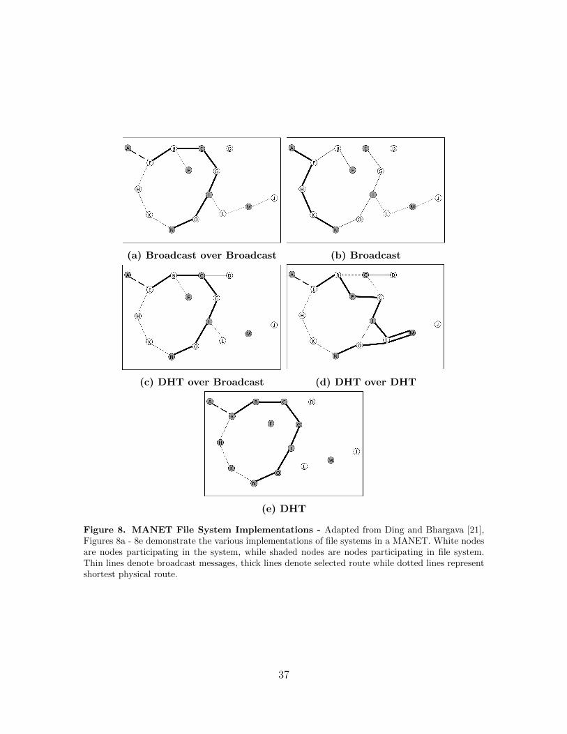
(a) Broadcast over Broadcast (b) Broadcast

(c) DHT over Broadcast (d) DHT over DHT

(e) DHT

Figure 8. MANET File System Implementations - Adapted from Ding and Bhargava [21],Figures 8a - 8e demonstrate the various implementations of file systems in a MANET. White nodesare nodes participating in the system, while shaded nodes are nodes participating in file system.Thin lines denote broadcast messages, thick lines denote selected route while dotted lines representshortest physical route.

37

2.5.2 Optimized Routing Independent Overlay Network (ORION).

The ORION protocol was presented by Klemm at el. as new approach to P2P

operation in MANETs [32]. ORION takes principles of AODV and other reactive

routing protocols and introduces it to the application layer. Instead of maintaining

static connections between peers, as in traditional P2P systems such as PASTRY

and Gnutella, connections are setup on-demand. Klemm states that while ORION

introduces potential for redundancy between the application and network layers, it

is possible to combine the two for cross-layer optimization. As such, ORION can be

implemented as either a Broadcast over Broadcast or Broadcast paradigm as listed

above. There are two principle divisions of ORION’s tasks, search and transfer.

2.5.2.1 ORION Search Protocol.

Each node in ORION hosts a local repository for files to share from its local

file system. The assumption is made that each file is uniquely identified. For its

application in the UAV Swarm problem domain, this is an important and reasonable

assumption. If each UAV is a separate sensor platform, it is reasonable and logical that

each file generated would be tagged with information about the UAV that generated

it; the time, location, and sensor type. This information would naturally be utilized

as a basis for search queries such as finding all imagery data of location x between

times y1 and y2, with obvious extensions to audio, video, infra-red, or any other

sensor utilized.

Each node also possess a response table and file routing table, similar to the tables

utilized by AODV, to manage current routes and RREQs. A Least Recently Used

replacement policy controls the size and memory consumption of the tables [32].

One primary difference between AODV and ORION, is that when files are re-

quested, the source is not looking for a particular node, it is looking for files that

38

Figure 9. ORION Query Broadcast - Node A initiates a query broadcast for file “c”. Onlynodes that do not contain the file re-broadcast the query. Nodes that receive queries only track thefirst arrived request with the same sequence ID. Notional file tables for nodes D,M, and O are shownin braces.

match its query criteria. To accomplish this, a QUERY message is broadcast in a

similar fashion to AODV’s RREQ. Nodes that own files that match the source node’s

query criteria reply with a RESPONSE message. Again, in line with AODV, each

message contains a SRC and SEQ field that is used to uniquely identify each request

and prevent loops. Figures 9 and 10 illustrate this process.

Figure 9 shows node A initiating a QUERY message, looking for file “c”. Node

A broadcasts a QUERY packet to its neighbors and they re-broadcast the QUERY.

Nodes that receive QUERY broadcasts only track the first arrived request with the

same sequence ID to prevent loops in the system. Furthermore, if a QUERY is

requesting a specific file, nodes only have to re-broadcast if they do not possess the

queried file. Using this broadcast attenuation technique can be useful for reducing

the traffic needed for re-querying during a failed transfer.

39

Figure 10. ORION Query Response - Nodes that possess file “c” respond to requests alongthe reverse path. Nodes add responses to their routing table for file “c”.

Figures 10 illustrates the process of nodes replying with a RESPONSE message.

Nodes that possess file “c” responds along the reverse path. Of course, this is a

simplified model, as the ORION protocol specifies that queries can be anything and

nodes can reply with any number of files that match the query criteria. If a node

receives a RESPONSE packet that contains a file listing that it already possesses, it

simply strips that file from the response before forwarding it along the reverse path.

2.5.2.2 ORION Transfer Protocol.

Due to the volatility of connections in a MANET, it is critical that control of

the transfer process resides at the requester (source) [32]. Since one assumption for

ORION is that nodes are homogeneous, and that the maximum transfer unit (MTU)

doesn’t vary between communicating nodes, files can be broken up into block sizes

40

that fit inside of a single packet. The source node, having a route to the desired file

and file information from the original QUERY message, initiates a DATA REQUEST

message for a single block to the corresponding node in its file routing table. When

the request reaches the provider node, it responds with a DATA REPLY message

that contains the file block.

ORION uses a local resolution for link-failure, which is a departure from the

AODV’s source initiated link-failure resolution protocol. In the event that a node

cannot fulfill the request for the file (it has no remaining entries in its file table) it

sends a ROUTE ERROR message back to the source node. At this point, the source

node can either abort the transfer or initiate a re-query. The only difference between

a re-query and a regular query message is that the source node is aware the file exists

in the network, and can request it by name instead of providing keywords.

The final piece of ORION’s transfer protocol is loss recovery and packet scheduling.

To handle the inevitability of drop packets, the transfer protocol uses a list of pending

block requests. When a file is first requested this list is initialized with all the block

required to complete the transfer (blocks = filesizeMTU

). To prevent unnecessary block

requests, the source node keeps track of the average round trip time and uses a round-

robin approach to requesting blocks. Therefore, all blocks in the file will be requested

before re-tries are attempted. Conducting the file requests in this round-robin fashion

allows time for the delayed blocks to still reach the source node before being requested

again.

2.5.3 ORION+.

ORION+ is an extension of the ORION protocol that was developed by Ahmed

Abada [1]. ORION+ attempts to improve the performance of ORION by using

proactive unicast messages to calculate link quality. According to the author, this

41

has the benefit of re-ordering routes based on quality instead of the first in approach.

Additionally, bad routes are determined before they are needed. ORION+ provides

no benefit if there is only one route to the requested file or the topology is changing

at a significant rate [1].

2.5.4 Mobile Peer-to-Peer (MPP) protocol.

While the author of ORION cites that it can be implemented as a cross-layer

solution, MPP is designed from the start to be exactly that [23]. However, the DSR

protocol is integral to MPP, such that every node participating in a MPP mesh must

be running DSR [1] where ORION will work on top of any protocol.

MPP has two types of transfer schemes, static and dynamic. With the static

mode, nodes involved in a file transfer file requests are cached for later use. When a

link breaks, the protocol will look up an alternate source from this cache. The static

mode is very similar to the ORION methodology. As Gruber points out, the static

system works well in systems with fewer nodes, low mobility, or small file sizes [23].

The dynamic mode of the protocol uses an first-come first-serve methodology

where the first route back from a file request is used. Any additional routes that

arrive afterward are discarded. In the event of a link failure, a new file request is

issued, thus re-flooding the network. The dynamic mode has the effect of using the

best source for the file until the link breaks (at the expense of more frequent network

flooding).

2.5.5 Availability Schemes.

Since a central part of this thesis is looking at the effect of redundancy, it is worth

our time to look briefly at some principles of replication. Tanenbaum and Van Steen

[50] states that redundancy, which is a key attribute to availability, can come from

42

two sources: replication and erasure coding. Replication, the most obvious solution,

entails creating duplicate copies on multiple nodes. When node availability decreases,

replication loses it ability to guarantee redundancy.

Erasure coding is the procedure of segmenting files into multiple fragments. Each

fragment contains additional information about the file, such that if multiple frag-

ments are missing, the file still can be reconstructed. Tanenbaum defines the redun-

dancy factor as rec = nm

, and the number of required m fragments to reproduce the

file is computed as

1− ε =n∑

i=m

(n

i

)ai(1− a)n−1 (3)

where m = number of fragments, a is the average node availability, ε is the required

file unavailability. The formula for calculating the replication rate for straight file

replication is

1− ε = 1− (1− a)rrep (4)

Taking these two formulas, Tanenbaum produces the ratio of recrrep

. When this ratio

is compared over the average percentage of node availability, straight file replication

requires twice as much redundancy as erasure coding to achieve the same guarantee

of file availability [50]. While this reduction isn’t that dramatic in a traditional

wired system, in a UAV swarm this represents a reduction in broadcast transmissions

(network congestion) and power consumption.

In traditional systems, file popularity is also an important concept. Intuitively,

the more popular a file is, the higher the replication rate should be. Increasing the

number of copies based on popularity ensures that the file is available as needed,

but also reduces the query time. Vranicar [52] uses Beehive [41] in this study of

data availability, but this system proves to be an unnecessary complication in our

stated problem domain. First, as Tanenbaum states, popular and uniform distribution

43

policies end up being very similar when looking at the average number of nodes that

need to be queried [50]. Second, in our system, once a file is retrieved there is no

further need for it. The file is extracted by the node with long-haul communication,

and as such, is really the only true consumer of files. In this sense, each node isn’t

really a “peer”, but simply a resource for the extraction node to utilize, so popularity

is null and void. However, if data availability is essential for operation of the swarm,

then a popularity based model could prove useful.

Chen looks at replication and MANETs with the goal of optimizing file availabil-

ity by reducing query delay. The optimization is done by calculating node meeting

frequency and using this parameter to adjust which nodes receive replications [18].

While an interesting proposition, Chen’s work does not take into account the issues

of placing increased demand on select nodes. The increased utilization will increase

network traffic to this node, potentially slowing routes requiring this node. Addition-

ally, the rise in traffic could increase the power consumption forcing it to be replaced

at more frequent intervals. For these reasons, a simple replication is better suited for

this thesis’s problem domain.

2.6 Simulation Environments

Since forming an actual network of UAVs is impractical for most research purposes,

most researchers turn to simulation as a means to study the various interactions of

interest. Discrete event simulators favored in the research papers present thus far

include QualNet, OPNET, GloMoSim, NS-2/3 and OMNeT++. While there are

many others, NS-3 and OMNeT++ are the main focus of this paper due to open-

source availability. Additionally, Koksal evaluated many simulators, and recommends

OMNeT++ and NS-2 as the best choices for researchers (NS-3 was not available at

time of his publication) [33].

44

2.6.1 Network Simulator Version 2/3.

Network Simulator Version 2(NS-2), begun as a project out of UC Berkly in

1997. For over a decade it received continued support from various sources due to

its open-source nature. NS-2 modules are written in C++ and it uses the OTcl

language for simulation scripting. NS-2 was the de facto simulator of choice for

many research papers. Network Simulator-3 is an open source discrete-event network

simulator that is the successor to NS-2. NS-3 was initially released in 2008 (and

still in active development) to improve the core architecture of NS-2 and provide a

pure C++ scripting environment where NS-2 was much more complex, dividing code

between C++ and OTcl. Its software core leverages object-oriented concepts such as

smart pointers and template programming to improve performance over NS-2. NS-3

also has a dedicated data-collection framework which provides robust data collection

capabilities. Unfortunately, the only application layer P2P module available to NS-3

is Pastry (at the time of this writing). Any additional file systems would need to be

coded as a separate module. NS-3 provides limited support for direct code execution,

allowing the simulation to interact with real programs and system processes as part

of the simulation. Additionally, NS-3 can also interact with real system process in a

real-time mode for testing of operational systems by supporting Berkley sockets and

POSIX threads [55] as well as provide the capability for evaluating packet traces with

network monitoring utilities such as Wireshark.

2.6.2 OMNeT++.

OMNeT++ is a discrete-event simulator that is utilized to run a variety of simula-

tion scenarios. For network simulation and experimentation, the INETMANET mod-

ules of OMNeT++ and Denacast P2P module are required. Denacast is an Oversim

(P2P simuation module) [9] adaptation to support MANET operation. Khan con-

45

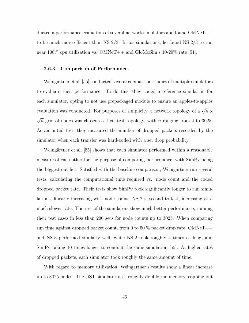
ducted a performance evaluation of several network simulators and found OMNeT++

to be much more efficient than NS-2/3. In his simulations, he found NS-2/3 to run

near 100% cpu utilization vs. OMNeT++ and GloMoSim’s 10-20% rate [51].

2.6.3 Comparison of Performance.

Weingartner et al. [55] conducted several comparison studies of multiple simulators

to evaluate their performance. To do this, they coded a reference simulation for

each simulator, opting to not use prepackaged module to ensure an apples-to-apples

evaluation was conducted. For purposes of simplicity, a network topology of a√n x

√n grid of nodes was chosen as their test topology, with n ranging from 4 to 3025.

As an initial test, they measured the number of dropped packets recorded by the

simulator when each transfer was hard-coded with a set drop probability.

Weingartner et al. [55] shows that each simulator performed within a reasonable

measure of each other for the purpose of comparing performance, with SimPy being

the biggest out-lier. Satisfied with the baseline comparison, Weingartner ran several

tests, calculating the computational time required vs. node count and the coded

dropped packet rate. Their tests show SimPy took significantly longer to run simu-

lations, linearly increasing with node count. NS-2 is second to last, increasing at a

much slower rate. The rest of the simulators show much better performance, running

their test cases in less than 200 secs for node counts up to 3025. When comparing

run time against dropped packet count, from 0 to 50 % packet drop rate, OMNeT++

and NS-3 performed similarly well, while NS-2 took roughly 4 times as long, and

SimPy taking 10 times longer to conduct the same simulation [55]. At higher rates

of dropped packets, each simulator took roughly the same amount of time.

With regard to memory utilization, Weingartner’s results show a linear increase

up to 3025 nodes. The JiST simulator uses roughly double the memory, capping out

46

at 140 MB. Weingartner evaluated memory consumption with respect to drop rate

probability and as expected, as packet loss goes up, less memory is required to track

current packets. It is important to note that the test case for this test was simple,

and more memory is expected to be utilized in a real network simulation. Based

on these results, both NS-3 and OMNeT++ are acceptable choices for this thesis’s

experimentation.

2.7 Summary

This chapter covered some of the core considerations in regards to operating a

Peer-to-Peer network in a MANET environment. A general overview of MANETs

was presented, followed by a quick description of the data-link layer protocols asso-

ciated with wireless communication. Extensive coverage of various routing protocols

was given to emphasize the importance of the network layer in intra-MANET commu-

nication. Routing protocols covered included proactive varieties such as DSDV and

OSLR, reactive protocols including AODV (and variants) and DSR. In addition, brief

coverage of hybrid protocols, virtual backbones, and quality of service considerations

was presented as well.

Chapter 2 also covered traditional P2P architecture, providing insight into how

distributed system are set up to transfer information in a traditional network, and

the challenges introduced by attempting to use the same methodology in a MANET.

The chapter then transitions to analyzing the five major paradigms for implementing

a P2P application in a MANET. Additionally, treatment was given to the MANET

P2P protocol that will be implemented as part of the experimentation in Chapter IV

(ORION), as well as the MPP protocol for comparison.

47

Finally, this chapter covered several simulation environments available for re-

searchers, compared performance, and assess validity. Next, Chapter III will present

the methodology in conducting the experiment.

48

III. Methodology

The objective of this experiment, is to ascertain the impact of replication on data

availability (as measured by mean query and transfer success rate and mean time for

request/delivery of information) in a mobile ad hoc network. Specifically, the experi-

ment is designed to measure the ability to extract information from a remote location

given a narrow-band communication channel and a given attrition/replacement rate

of unmanned aerial vehicles (UAVs) in the swarm. In particular, this experimental do-

main implements the Ad hoc On-demand Distance Vector (AODV) routing protocol

as the underlying ad hoc network and implements the Optimized Routing Indepen-

dent Overlay Network (ORION) protocol as its file replication/transfer mechanism.

Data will be collected from the simulation based on the ability of the swarm to

fulfill the request for information compared against the output provided by various

configurations. This experiment provides a combinatorial evaluation over four input

parameters. The evaluated parameters include: the number of nodes (i.e. UAVs

in the swarm), airspeed, replication level, and churn (i.e. attrition) rate. For each

configuration, twenty runs will be performed over 10 minutes of simulation time(i.e. 2-

4 thousand samples). The primary focus is on query and transfer success rates, while

secondary consideration is given to the speed at which the two primary objectives are

accomplished.

The replication amount/rate is important to study due to the increased traffic

generated from creating multiple copies on different nodes and how this impacts total

transfer time and availability. The hypothesis here is that as replication amount

increases, data availability (as measured by successful transfers) will increase until

network saturation is reached, at which point success rates will decrease and response

times will increase. The aim of this experiment is to identify the conditions under

which this trade-off between robustness and over-saturation occurs. Once a certain

49

level of replication is reached, transfer times will start to increase due to the amount

of traffic required to replicate the files, thus reducing available system bandwidth to

complete the file request. The key insight of this work is that increased replication

is expected to decrease transfer time initially due to the probabilistic decrease in

hop count from request origination to file source(s). In this way, multiple nodes will

be able to respond to the file request, thus ensuring a response to file requests and

consequentially improving data availability. Network utilization itself is not measured

explicitly as it has been covered extensively by Vranicar [52]. Interestingly, because

the only traffic generated in this system is either from the routing protocol or from

the application created for this experiment, we can attribute any change in response

time to the level of replication being employed by the swarm.

As noted by Andel and Yasinsac [6], many research papers suffer from a lack of

reporting on parameter specification. Andel and Yasinsac [6] examined many of the

publications on mobile ad hoc networks (MANETs) and found a gamut of issues. At

the time of their writing, 85% of the publications where not independently repeatable,

87.9% did not specify the version of simulator used, 30% did not specify simulator

package, 43% lacked transmission range specification, 65% did not list the number

of simulation runs, 87.5 % did not use confidence intervals, 71.6% did not list the

type of traffic utilized, and 61.5% did not use a mobility model [6]. Thus this chapter

also provides the information necessary to ensure the experiments are repeatable and

verifiable.

3.1 Experimental Design

The purpose of the experiment is to measure the impact of replication count on

an ad hoc peer-to-peer file system in relation to the availability of randomly selected

50

files and the end-to-end total transfer time. Several different control factors will be

evaluated, including: swarm size, node mobility (i.e. speed), and rate of churn.

3.1.1 Apparatus.

Since the experiment is conducted in a discrete time network simulator, it neces-

sary to discuss the system utilized for the experiment, (i.e. software and hardware).

3.1.1.1 Software.

OMNeT++ was selected for its open-source availability, robust network and mo-

bility models, efficiency, and ease of experimental integration. Final simulations were

performed on version 4.6, using INET (network simulation module) version 2.99.

Verification of simulator performance is critical when conducting experimentation

modeling real world scenarios. Bredel and Bergner [12] examine the performance of

the 802.11g wireless model in OMNeT++ and compare it to a real physical system.

They conclude that OMNeT++’s model performs very well over long observation

times with average measurements. They point out that discrepancies exist in packet

scheduling so care should be taken when analyzing “rare network events” [12]. Ivanov

et al. [27] examine the performance of NS-2, assessing its modeling of network con-

nectivity, packet delivery and latencies. Their work concludes that NS-2 does an

adequate job of modeling a multi-hop network in an indoor setting, but produced

mean latencies that were lower than real-world performance. The authors state that

this is most likely from two primary sources: lack of runtime overhead from the OS

and errors in dynamic data rate modeling (NS-2 uses static data rates). Their tests,

which consisted of measuring packets delivered as part of an MPEG-4 video stream

across 4 hops, found that the packet delivery ratio error averaged 0.3 to 1% of the

real world system. This work can be extended to NS-3 since the core models have

51

not changed between versions 2 and 3. These two works, when combined with the

comparison analysis of Weingartner et al. [55], lends credibility to the results of both

simulation environments (NS 2/3 and OMNeT++), with the understanding that no

simulation will ever be 100% accurate.

3.1.1.2 Hardware.

The simulations run on a 64-bit Intel Sandybridge i5-2500k quad-core processor

running at 3.7Ghz with 16 GB DDR3 RAM (pc-1600) on a ASUS ROG Maximum IV

motherboard, and a Samsung Solid State Drive (rated at 500MB/s read/write). The

test system OS is Windows 8.1 Pro with all foreground applications and unnecessary

services closed to prevent potential interference with testing.

3.1.2 Simulation Design.

The simulation scenario is defined by a set of nodes (i.e. UAVs) randomly moving

in a 1000 meter square bounded space using OMNeT++’s “mass-mobility” mobility

model. Upon reaching the edge of this region, the nodes are reflected back in at

the complementary angle. Each node, except the exfiltration (i.e. sink) node, will

generate a file at a set interval as to mimic nodes collecting some form of data (e.g.

imagery). Once the files are generated, they will attempt to replicate the file to its

closest neighbors based on the configured replication rate parameter, which varies

between 0 and 4. Periodically, the sink node (representing the node that possesses

the lower-bandwidth, long haul communication capability) will request one file at

random from the network as a whole. If a query response is not received within 1

second, the master node marks that file as unattainable and moves on to the next file.

The time to wait value was chosen empirically to maximize the number of samples

collected by the system, and should be adjusted to accommodate systems with higher

52

latency. Once the master node receives a response to the broadcast query (or times

out), it will request the file in accordance with the ORION protocol as detailed in

Chapter 2. Upon completion or failure of a query and transfer, the simulation adds

the requested file to a taboo list, thus ensuring the file is not requested again. The

simulation repeats the process until the simulation terminates at 600 seconds. In the

event that all generated files have been queried, the master node will sleep for an

interval equal to that of the file generation rate, giving the swarm time to generate

and replicate new files. Pending requests that occur when the simulation terminates

are discarded, resulting in a negligible loss that is not expected to have a significant

impact on results.

Transfer failures occur as either a timeout or a route error. In a timeout situation,

the file transfer request exceeds a set value of time allowed to complete the request.

For this experiment, this is set to 5 seconds. On the other hand, a route error is

generated when a node fails to receive a request acknowledgment from the next hop.

When a route error occurs, the unreachable node is removed from the receiving node’s

file source list, and sends a route error message to the previous node in the return

path. Subsequent route errors being performed recursively along the return path if

no other routes are available at each intermediate node.

If churn (i.e. nodes entering and leaving the system randomly) is enabled, a

percentage of nodes will be turned off for a set duration to simulate hardware faults,

UAV crashes, etc. During this window, the nodes will not reply to queries or transfers

until it is re-enabled. However, the node will continue to move (an effect that is not

expected to have a significant impact on results). When a node is selected to be

disabled, it turns of for a period of 30 seconds, meaning that it cannot act as a node

in the network, losing any previous data and routing info. This value was chosen

53

to be relatively large in network time to highlight the effect that churn has on the

system.

Since the focus of this thesis is on data availability resulting from replication

(rather than from layers 1,2, and 3 of the Open Systems Interconnect (OSI) model),

an idealistic radio model was chosen to represent the physical layer communication of

the network. This choice was made for simplicity and to limit the number of factors

in experimental design.

3.2 Assumptions

Several assumptions were made in the design of this experiment: Nodes are re-

placed at the same rate of attrition (i.e. churn rate), byzantine faults [50, 325] do

not exist, communication channels are secure and available, hardware errors do not

exist within the nodes unless that node is selected for attrition, individual nodes are

fully cooperative, nodes are homogeneous (i.e. equally compatible/capable), each file

is unique (data consistency checks are not required), each node possesses sufficient

storage capability, and finally, once a file has been extracted from the swarm, it will

not be requested again.

With that in mind, we can turn our attention to examining the response variables

that the experiment will measure.

3.2.1 Response Variables.

The experiment is conducted as a discrete time simulation with the following

parameters (Table 2).

• Query Success Rate (querySuccRate)- Measured as a ratio of the number of

queries completed versus the number initiated.

54

• Query Response Time (queryTime) - Measured in milliseconds, this mea-

sures the amount of time it takes for the source node to receive a response to

a request for a file. It includes the time required for the system to locate a file

and send the first response back to the source node. While multiple nodes may

be able to respond (due to replication), only the first response is measured.

• Transfer Success Rate (xferSuccRate) - Measured as a ratio of number of

completed file transfers over the number of file queries.

• Transfer Completion Time (xferTime) - Measured in milliseconds, this mea-

sures the amount of time it takes to complete a file transfer, not including the

initial query.

• Hop Count (hopCount) - Covariant, this measures the average number of

nodes query and transfer packets travel through from source to destination.

3.2.2 Independent Variables.

Due to the number of factors that can be varied in a simulation environment, this

experiment performs a full factorial experiment [37] over the following four factors

(Table 3).

• Replication Rate - The number of times an individual file is replicated to

other nodes across the system. Replication rate will remain constant value for

each run, but will be varied from 0 - 4 on different runs.

• Number of Nodes - The number of UAVs in the system under test. The node

count will remain constant during individual runs, independent of replication

rate. Node counts of 30, 45, and 60 are applied to simulate a small, medium,

and large UAV swarms.

55

• Speed - The rate of motion (i.e. UAV speed) is held constant for each run, but

is varied to 2, 8, and 15 meters per second between runs to evaluate the effect

of speed on network performance.

• Churn Rate - The churn rate factor how often nodes are removed from the

system and replaced with a new, blank node. To simulate nodes entering and

leaving the system for logistical reasons (e.g. fuel or maintenance) or catas-

trophic reasons (e.g. crashing). Churn rate values will be set to a constant 0,

5, or 10% for each run and will not effect the number of nodes.

3.2.3 Control Factors.

Across all runs of the experiment, several factors are held constant to limit the

scope of the experiment. While variations in these values would certainly impact the

system performance, they are not the focus of this research. (Table 4) summarizes

the experiment’s constant factors.

• Mobility Model - This factor describes how nodes move in the simulation

space. For this experiment, the Mass-mobility model included in OMNeT++ is

used rather than the typical random waypoint model used to simulate pedestrian

traffic. The Mass-mobility model’s continuous travel pattern more accurately

reflects the movement of a UAV swarm.

• Movement Space -Represented as a two-dimensional Cartesian coordinate

grid measured in meters, the simulation space is set to 1,000 meters for all

simulation runs. This value, along with number of nodes, dictate connection

density.

• Wireless Model - The simulation model used to represent the physical char-

acteristics of the wireless transmission. For the purpose of this experiment,

56

the IdealRadio Model included in OMNeT++ is chosen. It is not affected by

random errors, signal-to-noise loss ratios, and other anomalies.

• Transmit Rate - The data rate at which the simulator makes network con-

nections. OMNeT++ supports a variety of wireless protocols natively. This

experiment assumes an 802.11 wireless network with a bandwidth of 11Mbps.

• Transmit Range - The range at nodes are able to establish network connec-

tions. Keeping with the 802.11n standard, a value of 250m was chosen.

• Routing Protocol - AODV was chosen as the layer 3 routing protocol for all

runs in this experiment.

• File Size -The size of the data file to be transfered. This value is set to 100KB

across all runs as not to affect transfer times.

• File Generation Rate - The rate at which files are created on each node, and

is also used to determine how long the master node will sleep for in the event

that it has no new files to query. Throughout all runs, a generation rate of 3

seconds is used with node start times staggered randomly between 0 and 200ms.

• Churn Duration - The amount of time that nodes selected for attrition will

remain disabled. A value of 30 seconds is applied in all runs.

• Query Timeout - The amount of time before a query is considered to have

failed. A duration of 1 is utilized for all runs of this experiment.

• Data Packet Timeout - The amount of time before a transfer is considered

to have failed. A transfer timeout of 2 seconds is used for all runs.

• Requery Attempts - The number of times the transfer protocol will attempt

to transfer the file if a previous transfer fails. A value of 5 was selected based

57

on testing to provide reasonable results without attempting to overcome all

network failures.

3.2.4 Data Collection and Reduction.

Data is collected via a comma delimited log file. Each measurement taken or

calculated is recorded as both raw and summary data.

3.3 Summary

This chapter documented the experiment design and implementation that will be

used to evaluate the effects of file replication on data availability in ad hoc networks.

Specifically, this experiment is designed to evaluate the effects of replication count,

node count, node speed, and churn rate on a simulated ad hoc network’s ability to

access information in the network. Chapter IV presents the data collected from this

experiment and provides insight into factor interaction.

58

Table 2. Response Variable Summary

Response variable Normaloperatinglevel andrange

Measurementprecision

Relationship of re-sponse variable toobjective

querySuccRate 0-100 % calculated ratio Measured as a ratio of num-ber of queries for files to thenumber of responses.

queryTime 0-100 ms 1 ms steps, mea-surement basedon simulationclock. Priorresearch servesas baseline

It includes the time it takesfor the system to find afile in the network and thensend the first response backto the source node. Sincemultiple nodes may have acopy of the requested file,only the first response backis measured.

xferSuccRate 0-100 % calculated ratio Measured as a ratio of num-ber of requests for a fileto number of completed filetransfers.

xferTime 0-5000 ms 1 ms steps, mea-surement basedon simulationclock.

Amount of time it takes tocomplete a file transfer. Itdoes not include the timefor the initial query.

hopCount 0-10 averaged value average number of nodesa query or transfer travelsthrough.

Table 3. Independent Variable Summary

Independent Variable NormalOperatingLevel

Proposed Settings Predicted effects

Replication Rate 0-10 0-4 DifferenceNumber of Nodes 0-150 30, 45, 60 unknown

Speed 0-25 m/s 2, 8, 15 DifferenceChurn Rate 0-100 % 0%, 5%, 10% Difference

59

Table 4. Constant Factors Summary

Factor Desired experimental level How Controlled?

Mobility Model Mass-Mobility Sim ConfigurationMovement Space 1000 x 1000 m Sim ConfigurationWireless Model IdealRadio Sim Configuration

Transmission Rate 11MB/s Sim ConfigurationTransmission Range 250m Sim Configuration

Routing Protocol AODV Sim ConfigurationFile Size 100KB Sim Configuration

File Generation Rate 3s Sim ConfigurationChurn Duration 30 s Sim ConfigurationQuery Timeout 1 s Sim Configuration

Data Packet Timeout 2000 ms Sim ConfigurationRequery Attempts 5 Sim Configuration

60

IV. Results and Analysis

The primary objective of this research is to evaluate the impact of file replication

on availability, with a secondary look at the impact on transfer and query rates in a

simulated mobile ad hoc network (MANET). The following results of the simulation

and analysis will be examined as an aggregate collection, then a deeper look will

be given by breaking out the results based on the simulation factors. As a last

look, results with respect to time will be investigated to investigate the possibility

of measurement time playing a factor in results. The granular breakdown is done to

provide a deeper analysis of how the simulation factors impact the overall results.

The data presented in this chapter was analyzed using the “R” statistical program.

Line graphs have been chosen to represent the data with confidence intervals for each

data point. These graphs are generated using the ggplot library [56].

4.1 Aggregate Values

When measuring availability, this thesis looks at two primary components, first

whether or not the system can locate the file in the network, and second, the ability of

the system to successful transfer the file (ex-filtration). Query success rate measures

the first component, and transfer success rate measures the second factor. Since

the main goal of this thesis is to evaluate the impact that file replication has on

availability, query and transfer success rate will be examined first as an aggregate

collection of factors. The time to execute queries and transfers, secondary objectives

of this thesis are also presented. Inspecting the results with respect to node count,

mobility and churn rate will be broken out further in the chapter.

61

4.1.1 Query Success Rate.

Figure 11 illustrates query and transfer success rates based on the replication

count. Looking first at the query success rate, the top left chart clearly shows that

replication induced a significant effect on the ability of the unmanned aerial vehicle

(UAV) swarm to locate a file. Increasing replication from 0 copies of the file to 1

copy, the mean query success rate increased from of a baseline 76.3% to 85.4%, for a

mean query success rate increase of 9.1%. Increasing the replication rate to a factor

of 2 resulted in a much smaller increase of 3.13% (85.4 to 88.6 success rate) from a

replication level of 1. Further increasing the replication factor to 3 only results in a

gain of 1.17% over a replication factor of 2. Finally, a replication factor of 4 actually

decreases the query success rate by 0.62% from the value obtained by the replication

factor 3 measurements.

4.1.2 Transfer Success Rate.

Knowing that the file exists is one part of the equation. Successful extraction

of the file from the swarm, after ascertaining its existence, is the other part. The

top-right illustration in Figure 11 displays the combined results of all factors for

transfer success rates based on replication levels. As expected, the transfer rate

closely follows the query success rate pattern, but at a lower rate of success. The

baseline (replication factor of 0) mean transfer success rate is 62.65%. Increasing the

replication factor to a value of 1 results in a mean transfer success rate increase of

10.81%. Adding an additional replication (replication factor of 2) increases the mean

transfer success rate from 73.46% to 77.12% (increase of 3.65%). A replication factor

level of 3 nets an additional 1.18% increase in transfer success rate over the replication

level 2 measurements. Finally, as with the query success rate, the measured transfer

success rate decreases when the replication factor is set to a value of 4. Additional

62

●

●

●● ●

0.00

0.25

0.50

0.75

1.00

0 1 2 3 4Replication Count

Mea

n Q

uery

Suc

cess

Rat

e

Query Success

●

●

●●

●

0.00

0.25

0.50

0.75

1.00


Mea

n Tr

ansf

er S

ucce

ss R

ate

Transfer Success

●

●●

●

●

0

5

10


Mea

n Q

uery

Tim

e (m

s)

Query Time●

●

● ●

●

0

200

400

600


Mea

n Tr

ansf

er T

ime

(ms)

Transfer Time

Figure 11. Query/Transfer Success Rates and Mean Time (All Nodes) - This group ofcharts shows the overall agrigated means across all node counts, speeds, and churn rates for eachreplication factor with 95% confidence intervals overlaid. The upper-left illustrates mean querysuccess rate while the upper-right shows mean transfer success rates. On the bottom, the left chartsthe mean query time for each replication factor while the right shows mean transfer time. Theaggregrate data shows a general improvement in availability as replication goes up to a factor of 3,but starts to decrease at a factor of 4, with the inverse being true for query and transfer times.

63

replication resulted in a mean transfer success rate decrease of 2.31% to (from 78.31

to 76.0%).

4.1.3 Query Time.

The lower left graph of Figure 11 shows the impact of replication on mean query

time. Its quite obvious that replicating files once has a significant impact on mean

query time, decreasing mean query time by 41.53%. Further replication however,

has no statistically significant effect. It should be noted that while this reduction is

significant based on percentage, this impact is trivial in a system where large files

are transferred, as a query only requires 1 packet to be broadcast, versus the many

packets required to transport the data. However, if many smaller files are to be

transferred (suggesting more queries will be performed), this measurement becomes

more significant

4.1.4 Transfer Time.

A secondary objective of this thesis is to examine the impact of file replication on

mean transfer time of queried files. The bottom-right graph illustrates the effect of

replication on transfer time. As can be seen, increasing replication from 0 to 1 im-

proves (decreases) mean transfer time by 59.60 ms. The mean transfer time is further

reduced by an additional 27.16 ms. Further increases in replication fail to result in a

significant decrease in transfer time, and in fact start to increase the transfer time as

replication count is increased to 4. The lack of improvement with increased replica-

tion would suggest that the amount of network traffic required to achieve this level

of replication impacts the speed of the file transfer protocol. The delay is assumed

to be the result of UDP packet retransmissions due to network broadcast congestion.

64

Additionally, packet queue lengths are suspected of contributing to this delay, but

analysis of packet queues are outside of the scope of this research.

4.2 Results by Node Count

Now that the combined measurements have been examined, results based on

swarm size (with values of 30, 45, and 60) will be examined to ascertain what impact

swarm size (or node count) has on performance. It should be noted that node speed

(mobility) and churn rates are aggregated in these measurements.


Looking at mean query success rate (top-right, Figure 12 ), it is clear that the

30 node swarm is at a significant disadvantage in completing query requests with

respect to larger swarms. At the baseline value of zero replication, the 30 node swarm

possesses a mean query success rate approximately 20% lower than the medium and

large swarm. The difference between values is most likely caused by the average node

density of the coverage area. Smaller networks are more likely to become disconnected

and therefor less likely to be able to successfully complete the requested query. The

smaller swarm shows an increased improvement in query completion over the medium

and large node swarms as the replication factor is increased to 1. Further increases

in replication show slight gains in query success rate at replication factors 2 and 3

and performance starts to decrease when replication is set to 4 for all swarm size

sample groups. Analysis of Variance (ANOVA) of the complete data set shows that

all factors have a statistically significant impact on query success. The ANOVA data

can be seen in Table 5. However, as shown in Table 5, the size of the swarm has the

most dramatic impact (based on the F-statistic values).

65

●

●● ● ●

0.00

0.25

0.50

0.75

1.00


Mea

n Q

uery

Suc

cess

Rat

e

Query Success

●

●● ●

●

0.00

0.25

0.50

0.75

1.00


Mea

n Tr

ansf

er S

ucce

ss R

ate

Transfer Success

●●

●

●

●

0

5

10

15


Mea

n Q

uery

Tim

e (m

s)

Query Time

●

●● ● ●

0

200

400

600


Mea

n Tr

anns

fer

Tim

e (m

s)Transfer Time

Nodes

● 30

45

60

Figure 12. Query/Transfer Success Rates and Mean Time by Nodes - This figure is thesame format as 11, but mean values are separated by the node count factor. The 30-node swarmmaintains an approximate 20% reduction in query and transfer success. The lower left shows thesmall swarm not following the general trend of the larger node swarm.

Table 5. ANOVA for Query Success

Df Sum Sq Mean Sq F value Pr(>F)

Replication 4 1856 464.06 4255.34 0.00000Speed 2 152 76.11 697.93 0.00000Nodes 2 3946 1972.87 18090.87 0.00000Churn 2 3429 1714.41 15720.85 0.00000Residuals 740103 80711 0.11

66


Similar results are demonstrated in mean transfer success rate values, albeit at a

reduced success rates. The top-right and bottom-right charts of Figure 12 shows an

almost identical trend line between nodes for mean transfer success and mean trans-

fer time for all node counts, implying that changes in replication count impact all

swarms similarly, regardless of swarm size. Turning to ANOVA analysis of transfer

success rates (Table 6), we can see a slightly different picture than what transpired

with query success rates. The ANOVA data shows that when it comes to successfully

completing transfers, node mobility plays a more important role than node count.

Surprisingly, the replication factor, while still statistically significant, is least impor-

tant when examining all factors together.

4.2.3 Query Time.

A particular measurement of interest when looking at the data broken out by node

count is the mean query time. With respect to the 30 node swarm, mean query time

monotonically increases when replication count is increased, where as in the larger

swarms, query time first decreases up to a replication count of 3 and then starts

to trend upward. The upward trend is more pronounced in the lower node count

swarms. It is suspected that the difference with the small swarm is that since such

a smaller number of queries are successful, the query time measurement is skewed

by a difference in amount of measurements taken. It is also presumed that queries

that were successful took place in a cluster of nodes where increasing replication

would generate a localized network saturation, thus increasing the delay in sending

responses.

67

Table 6. ANOVA for Transfer Success

Df Sum Sq Mean Sq F value Pr(>F)

Replication 4 2386 596.48 3416.84 0.00000Speed 2 5630 2815.21 16126.52 0.00000Nodes 2 3605 1802.30 10324.19 0.00000Churn 2 3443 1721.28 9860.07 0.00000Residuals 740103 129200 0.17

4.2.4 Transfer Time and Hop Count.

The smaller swarm has the benefit of having to search fewer nodes, and there-

fore increasing the probability that the file is found in fewer hops (failures do not

play a factor here). However, since only successful queries are evaluated, the smaller

swarm is more likely to have network disconnects at longer hop counts. In the larger

swarms, it is more likely the file is located at a greater number of hops from the source

(most likely due to more successful queries being measured). Increasing replication

decreases the mean hop count and therefor decreasing mean query and transfer times.

However, just as was shown before, once replication reaches a point of network satu-

rations, response times increase and override the gains achieved by reducing the hop

count. Figure 13 shows these two measurements side by side. Figure 13a shows the

effect of replication on mean hop count. Increasing the replication factor reduces the

mean hop count almost uniformly across node count samples. Figure 13b shows the

corresponding transfer time tracking very closely to the mean hop count.

4.2.5 Total System Packets.

While looking at the experiment data separated by node count, it would be worth-

while to comment on the total number of application level packets used at the various

levels of replication. Figure 14 shows the linear increase in the mean sum of appli-

cation packets generated by each configuration. Obviously, at a replication factor of

zero, relatively few packets being generated. Any variance in the number of pack-

68

●

●

●

●

●

0

1

2

3


Mea

n H

ops Nodes

● 30

45

60

(a) Hop count

●

●

● ● ●

0

200

400

600


Mea

n Tr

anns

fer

Tim

e (m

s)

Nodes

● 30

45

60

(b) Transfer time

Figure 13. Mean Hop Count and Transfer Time by Node Count - Increasing replicationdecrease the mean hop count for each sample group. The transfer time follows the hop count trenduntil a factor of 3 is reached.

ets is caused by how the system is designed to initiate queries. To maximize the

number of data points, as soon as a query and transfer is complete, the next one is

initiated; therefore in systems where network dynamics induce slower requests, fewer

measurements will be made, and therefore fewer packets generated. As the replication

factor is increased, the amount of packets increases based on the number of nodes

in the swarm, the number of packets required to query and transfer the file for each

replication, and additional packets for retransmission as needed.

4.3 Results by Mobility

The following section examines the experiment sample data based on node speed

(mobility). It is important to note that node count and churn rates are aggregated

in these measurements.

69

●

●

●

●

●

0

5000

10000

15000


Mea

n To

tal S

um o

f App

licai

ton

Leve

l Pac

kets

(th

ousa

nds)

Nodes

● 30

45

60

Figure 14. Mean Total Sum of Applicaiton Level Packets - The total number of applicationlevel packets increases linarly with respect to node count as replication level is increased.

70


Another factor to examine is how node mobility affected availability. Looking at

the top-left chart in Figure 15, it is apparent that varying node mobility has little

impact on the mean query success rate. In contrast, varying node mobility did in

fact have a significant impact on transfer success. At the lowest speed factor (2 m/s),

increasing replication monotonically increases the mean transfer success rate. Again,

as expected, the largest increase being realized with the first and second replication

factor increase. The 8 and 15 m/s factor samples show a more pronounced increase

in success rate as replication is increased from 0 to 3 in the 8 m/s sample group

and 0 to 2 in the 15 m/s sample group, above which, increasing replication reduces

mean success rate by 3.05 and 6.16%, respectively. Logic would suggest that the

increase in mobility resulted in an increase in the number of retransmissions required

due to broken links. The data here suggests that a similar trend would be seen in

the 2 m/s mobility group at a higher replication count, however this would need to

be measured in a separate experiment. Finally, an interesting observation is that in

the slowest sample group, the mean transfer success rate tracks very closely with the

mean query success rate, whereas in the faster mobility groups, mean transfer success

is significantly impacted due to the increase in mobility.

4.3.2 Query and Transfer Time.

The mean amount of time required to complete a successful query is visualized

in the bottom-right of Figure 15. Increasing replication count from 0 to 1 slightly

reduced the mean query time of the 2 m/s sample group, but had no significant impact

beyond that. At the higher speeds, increasing replication rate had a larger impact

on mean query time, reducing mean query time by 1.52ms, 6.48ms, and 9.66ms for

the 2, 8, and 15m/s sample groups, respectively, as replication increases from 0 to

71

1, but again we see that further increases start to negatively impact the mean query

time. What is apparent from this chart is that node mobility has a clear and distinct

impact on mean query time, much more so than replication rate. It is suspected

that packet routing plays a key factor in this delineation, but further research is

required to make certain of this suggestion. As for the mean transfer time, increasing

mobility has little impact below a replication factor of 1. As replication is increased

beyond 2, mean transfer time is impacted negatively, albeit slightly. It should be

noted that unlike the samples separated by node count, mean query and transfer

times are inversely ordered in the mobility grouped samples. Counter to intuition,

the faster moving swarm has a slight advantage in terms of transfer speed (when only

considering completed transfers). The reason for this becomes apparent when the

mean hop count for each group is examined.

4.3.3 Hop Count.

Figure 16a shows that increasing the mobility of the swarm has the positive effect

of reducing the mean hop count for each transfer. The mean transfer time can be

viewed with respect to the mean hop count in Figure 16b. The 15 m/s swarm has the

lowest mean hop count per replication factor, while the 2 m/s swarm has the highest

mean hop count.

It is prudent at this point to discuss how the mean hop count is calculated. For

each measurement transfer (does not include transfers between nodes for replication)

that takes place, each file block that is received tracks the number of hops it traveled

to get from source to sink. When the completed transfer is recorded, the number

of total hops is divided by the number of blocks, giving a mean hop count for that

transfer. Only the first data packet for each block is counted, as duplicate packets are

discarded if the block has already been received. Also, if a transfer is not completed

72

●

● ● ● ●

0.00

0.25

0.50

0.75

1.00


Mea

n Q

uery

Suc

cess

Rat

e

Query Success

●

● ● ● ●

0.00

0.25

0.50

0.75

1.00


Mea

n Tr

ansf

er S

ucce

ss R

ate

Transfer Success

●● ● ● ●

0

10

20


Mea

n Q

uery

Tim

e (m

s)

Query Time

●

● ● ● ●

0

200

400

600


Mea

n Tr

ansf

er T

ime

(ms)

Transfer Time

Speed

● 2

8

15

Figure 15. Query/Transfer Success Rates and Mean Time by Speed - The top-left chartshows a close grouping of values, indicating that node mobility does not play a significant role inquery success. The top-right and bottom-left charts show a clear seperation of trend lines, showingthat contrary to query success, node speed does factor into transfer success rates and mean querytimes.

73

●

●

●●

●

0

1

2

3


Mea

n H

ops Speed

● 2

8

15

(a) Hop count

●

●●

●●

0

200

400

600


Mea

n Tr

ansf

er T

ime

(ms)

Speed

● 2

8

15

(b) Transfer time

Figure 16. Mean Hop Count and Transfer Time by Speed - Increasing replication decreasethe mean hop count for the sample groups based on mobility . The transfer time follows the hopcount trend until a factor of 3 is reached.

successfully, it is re-attempted up to 4 additional times before being considered a

failure. System implementation is a possible explanation as to why the higher mobility

swarm possesses a lower mean hop count, even at a replication factor of 0. At higher

levels of replication, it is suspected that in the higher mobility swarms, the faster

mobility results in a quicker diffusion of replicated files, increasing the likelihood that

a node containing the requested file is closer to the requester (sink).

4.4 Results by Churn

A critical piece of of this experiment is to determine how replication affects avail-

ability given different levels of attrition. To achieve this, nodes where “turned off”

for a set duration of time. The number of nodes turned off was a percentage of the

swarm size. While turned off, all of the disabled nodes’ data tables were erased so

when they are re-enabled, it was the equivalent of being replaced with new nodes.

Below is the results of the experiment when examined with respect to churn rate.

74

The churn rate is maintained at a steady rate for the duration of the experiment,

with nodes being “turned on” before new nodes are chosen to be disabled.


The top-left graph in Figure 17 shows the mean query success rates grouped by

churn rate. Obviously, when the churn rate factor equals 0, the system has a very

high probability of successfully querying a particular file. Increasing the replication

level from 0 to 1 slightly increases the query success rate by 1.66%. The impact of

replication on node availability when zero churn is present is dampened by the fact

that the larger swarms (45 and 60 nodes) already had relatively high success rates

at a 0 replication level (80.76 and 82.38%, respectively) when higher churn rates are

factored in. As churn rate increases, the baseline mean query success rate is lowered

to 73.7% at a 5% churn rate, and 59.88% mean query success rate at 10% churn rate.

As replication is increased by a factor of one, query success rates improve by 1.66,

13.14, and 15.02% for the 0, 5, and 10% churn rates, respectively. As expected, the

higher churn rates realize a greater improvement in availability as measured by mean

query success rate. These gains have diminishing returns as replication is increased

further. With 0 churn, increasing replication does not significantly improve mean

success rate. Gains taper off once a file is replicated twice in the 5% churn samples

and at a factor of 3 in the 10% churn grouping.


Mean transfer success rate trends follow very closely to the mean query success

rate trends when grouped by churn rate. Again, we see transfer rates improving as

the replication factor is increased only to start degrading once reaching a certain

replication factor. When there is zero churn in the system, mean transfer success

75

● ● ● ● ●

0.00

0.25

0.50

0.75

1.00


Mea

n Q

uery

Suc

cess

Rat

e

Query Success

●● ● ● ●

0.00

0.25

0.50

0.75

1.00


Mea

n Tr

ansf

er S

ucce

ss R

ate

Transfer Success

●

● ● ●

●

0

5

10

15


Mea

n Q

uery

Tim

e (m

s)

Query Time●

●● ●

●

0

200

400

600


Mea

n Tr

anns

fer

Tim

e (m

s)

Transfer Time

Churn

● 0

5

10

Figure 17. Query/Transfer Success Rates and Mean Time by Churn -Churn rate has animpact on query and transfer success rates as indicated by the top figures, while less of an impactis seen in query and transfer times (bottom charts).

rates increase from 75.13% to 83.25% at a replication factor of 2, 83.54 at replication

factor 3, and starts to degrade at a factor of 4 only completing 81.3% of transfers.

Likewise, at a churn rate of 5%, the baseline transfer success is 60.45%, increasing to

78.77% at a replication factor of 3 and degrades to 77.2% at a replication factor of

4. In a system with a 10% churn rate, without replication, the experiment measures

a mean transfer success rate of 48.83%. Mean transfer success rate improves 14.47%

when replication factor is set to 1 and peeks at 70.24% at a replication factor of 3,

before decreasing roughly 2% at a replication factor of 4.

76

4.4.3 Query Time.

As seen in the bottom-left graph in Figure 17, increasing replication dramatically

impacts the query time in the sample group with zero churn, reducing mean query

time by 50% (13.3 to 6.64). However, after this initial increase, further replication

does not change query time by any level of statistical significance. Similar reductions

in mean query time are exhibited in the 5 and 10% churn sample groups at a lower

improvement rate (39.4 and 22.5%, respectively). In the higher churn sample groups,

increasing replication beyond a factor of 1 leads to a trend in increasing mean query

time, with a more pronounced effect in the 10% churn sample group. Again, this

data points to network traffic overriding any gains seen by reducing hop distance

between requesting and source node. Overall, while statistically significant (analysis

of variance (ANOVA) shows a p-value of < 2e-16), churn rate is not as significant

factor when examined in the context of the overall system.

4.4.4 Transfer Time and Hop Count.

In regards to mean transfer time, it is clear from the lower-right chart in Figure

17 that churn has extremely limited impact when zero replication is being performed.

Intuitively, the low impact is a result of the fact that transfer times are only calculated

on successfully completed transfers. As before, if we examine mean transfer time

concurrently with mean hop count as in Figure 18, we can see that mean hop is

the driving force behind transfer times. In fact, with the exception of the replication

factor of 4 data points, the two charts show almost identical trend lines, giving further

support to the hypothesis that hop count drives transfer speed until it is overcome by

network congestion. In all churn sample groups, hop count monotonically decreases

as replication count increases, for a net reduction of 0.895, 0.776, and 0.623 mean

hops in the 0, 5, and 10% churn groups (respectively). Of note is that fact that in the

77

●

●

●

●●

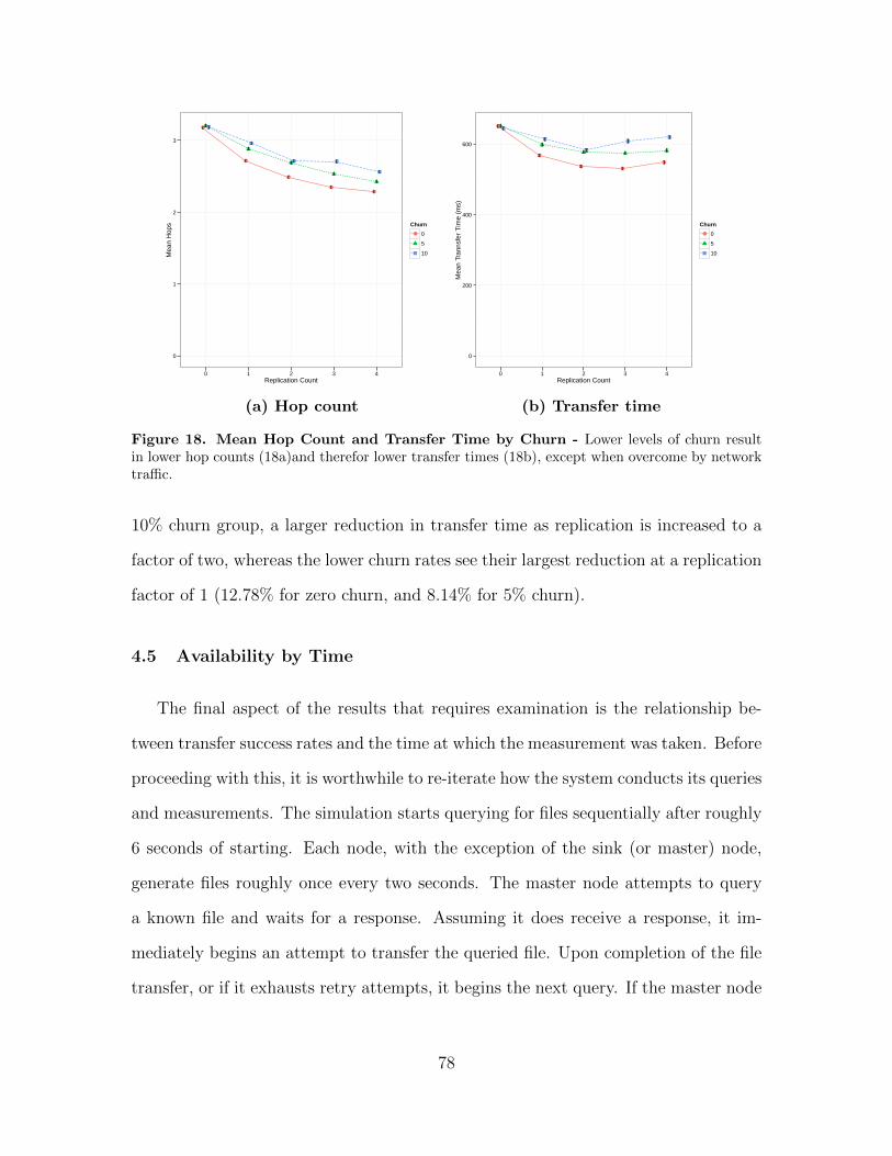
0

1

2

3


Mea

n H

ops Churn

● 0

5

10

(a) Hop count

●

●

● ●

●

0

200

400

600


Mea

n Tr

anns

fer

Tim

e (m

s)

Churn

● 0

5

10

(b) Transfer time

Figure 18. Mean Hop Count and Transfer Time by Churn - Lower levels of churn resultin lower hop counts (18a)and therefor lower transfer times (18b), except when overcome by networktraffic.

10% churn group, a larger reduction in transfer time as replication is increased to a

factor of two, whereas the lower churn rates see their largest reduction at a replication

factor of 1 (12.78% for zero churn, and 8.14% for 5% churn).

4.5 Availability by Time

The final aspect of the results that requires examination is the relationship be-

tween transfer success rates and the time at which the measurement was taken. Before

proceeding with this, it is worthwhile to re-iterate how the system conducts its queries

and measurements. The simulation starts querying for files sequentially after roughly

6 seconds of starting. Each node, with the exception of the sink (or master) node,

generate files roughly once every two seconds. The master node attempts to query

a known file and waits for a response. Assuming it does receive a response, it im-

mediately begins an attempt to transfer the queried file. Upon completion of the file

transfer, or if it exhausts retry attempts, it begins the next query. If the master node

78

exhausts all known files (file names are a function of node number and simulation

time, it is easy for the master to keep track of what files would have been generated),

it sleeps for 3 seconds to allow nodes time to generate new files. If a node is disabled

due to churn, any files that it would have normally generated are added to a taboo

list that the master node checks before querying for a file. How the query process

executes is vital to keep in mind as it leads to the concept that the older a file is, the

higher its risk of being lost due to node churn.

4.5.1 Grouped by Nodes.

Transfer success rate based on time of measurement will be examined by first

looking at these measurements with respect to swarm size. Figure 19 breaks this

down by first showing mean values with replication count values being aggregated for

each swarm size sample groups in Figure 19a. Trend lines indicate a steady gradual

reduction in mean transfer success for the 45 node swarm, with a net loss of 13.01%

over 540 seconds (a mean rate of 0.024% per second), and the 60 node swarm losing

10.5% at a mean rate of 0.19% per second. The 30 node swarm faces the same

reduction in mean transfer success rate, although the impact of time is a bit more

muted with the smallest swarm only losing 6.09% over the same time span. Figures

19b, 19c, and 19d show the breakdown of results by replication factor for each of the

three swarm size samples (30, 45, and 60, respectively). The 30 node swarm shows

more variation in mean rates, with increases in mean transfer success rates occurring

near the 300 and 600 second time intervals. Further investigation would need to be

conducted to examine this trend, although it is expected that this a result of the

mobility of the small swarm, and not related to replication, due to the trend being

present in varying degrees in all replication factors sample groups.

79

●●

● ●● ●

● ● ●

●

0.00

0.25

0.50

0.75

1.00

60 120 180 240 300 360 420 480 540 600Time of Measurement

Mea

n S

ucce

ss R

ate

Nodes

● 30

45

60

(a) By Node Count

●

●

● ●

●

●

●

●●

●

0.00

0.25

0.50

0.75

1.00


Mea

n S

ucce

ss R

ate Replication

● 0

1

2

3

4

(b) 30 Nodes

●

●

●

●

●●

● ● ●●

0.00

0.25

0.50

0.75

1.00


Mea

n S

ucce

ss R

ate Replication

● 0

1

2

3

4

(c) 45 Nodes

●

●

●

●●

●● ●

● ●

0.00

0.25

0.50

0.75

1.00


Mea

n S

ucce

ss R

ate Replication

● 0

1

2

3

4

(d) 60 Nodes

Figure 19. Mean Transfer Success Rate by Time, Replication, and Nodes - These chartsdemonstrate the impact of time of transfer on the mean transfer success rate. Figure 19a shows thiseffect with respect to swarm size, while Subfigures 19b - 19d break down each swarm size samplegroup further by replication count. With zero replication, mean transfer success rate decreasessignificantly over time, while this effect is attenuated to varying degrees by replication.

80

4.5.2 Grouped by Speed.

Just as was done for samples separated by node count, we can examine transfer

success rate based on the time of measurement and node mobility as shown in Figure

20. From Figure 20a its clear that speed is an definitive factor. At 2 m/s, the mean

transfer success rate drops by 11.62%. At 8 m/s, the mean transfer rate decreases by

10.17%, while at 15 m/s, the mean transfer success rate drops by 7.69%. Of course,

the inverse relationship between speed and transfer success still stands. Aside from

the baseline drop in transfer success rate based on increased speed, the time of the

measurement appears to have the same impact. Figures 20b, 20c, and 20d show the

results broken out by replication factor. One of the more interesting observations

how replication affects transfer success rates at different speeds. At 8 m/s and 15

m/s we can see that setting the replication to a factor of 3 results in the highest

levels of availability, however, at 15 m/s setting replication to a factor of 4 reduces

its success rates to that below a replication factor of 2. This trend matches what is

shown in top-right chart in Figure 15, and demonstrates that swarm size alone does

not account for all increases in network traffic.

4.5.3 Grouped by Churn.

Figure 21 shows the measurements broken down by the added time component.

Figure 21a shows mean success rates based on churn rates (with all other factor levels

aggregated). Clearly churn rate has a detrimental impact on the ability to transfer a

randomly selected file. 60 seconds into the simulation, all sample groups maintain a

similar transfer success rate of roughly 80%. However, as simulation time progresses,

the higher the churn rate, the greater the decrease in mean transfer success rate.

This reduction is intuitively due to the fact that as churn rate increases, the higher

the likelihood that all nodes that contain a copy of the file are eliminated from the

81

●●

● ●● ●

● ● ● ●

0.00

0.25

0.50

0.75

1.00


Mea

n S

ucce

ss R

ate

Speed

● 2

8

15

(a) By Speed

●

●

●●

● ●●

● ● ●

0.00

0.25

0.50

0.75

1.00


Mea

n S

ucce

ss R

ate Replication

● 0

1

2

3

4

(b) 2 m/s

●

●

● ●● ●

● ● ●●

0.00

0.25

0.50

0.75

1.00


Mea

n S

ucce

ss R

ate Replication

● 0

1

2

3

4

(c) 8 m/s

●

●●

●● ●

●●

● ●

0.00

0.25

0.50

0.75

1.00


Mea

n S

ucce

ss R

ate Replication

● 0

1

2

3

4

(d) 15 m/s

Figure 20. Mean Transfer Success Rate by Time, Replication, and Speed - Following thesame format as Figure 19, these charts demonstrate the impact of time of transfer with respect tonode mobility and replication. At lower speeds, higher levels of replication can be utilized to increasetransfer success rate. No significant variance exists between sample groups with respect trends overtime.

82

system as the system does not make an attempt to re-copy files after nodes have

been eliminated. As expected, the success rate for the 0% churn sample group stays

relatively constant throughout the full duration of the experiment. Figures 21b, 21c,

and 21d go a step further and break down the individual churn rate factors based

on replication rate. Looking only at samples where the churn rate factor is set to

zero (Figure 21b), it is evident that replication improved availability, but as seen in

data already presented, increasing replication beyond a factor of 2 proves to improve

availability trivially.

Increasing churn to 5% as illustrated in Figure 21c shows a definitive impact on

mean transfer success rate. By increasing replication to a factor of 1, a mean gain

of 14.34% in transfer success rate is achieved over no replication. Further increasing

replication to a factor of 2 nets an addition increase of 4.26%.

Figure 21d shows the results over time when churn rate is set to 10%. As expected

the system experiences a significant drop off in transfer success rates when no repli-

cation is present. The trend line suggests that the system stabilizes at a minimum

success rate of approximately 32%, although additional runs with a longer duration

would be required to determine if this is in fact the case. The stabilization rate is a

function of file generation speed, mean query/transfer speed (file size being a factor)

and churn rate. Incrementing replication rate by 1 improves transfer success rate by

14.97% and setting replication to a factor of 2 further improves transfer success rate

by 5.54%, and by 2.07% at a replication factor of 3. As a reminder, these percentages

are reported as a mean value, averaged over the duration of the entire simulation run.

83

● ●● ● ● ●

● ● ● ●

0.00

0.25

0.50

0.75

1.00


Mea

n S

ucce

ss R

ate

Churn

● 0

5

10

(a) By Churn Rate

● ●

●●

●●

● ● ● ●

0.00

0.25

0.50

0.75

1.00


Mea

n S

ucce

ss R

ate Replication

● 0

1

2

3

4

(b) 0% Churn

●

●

●

●●

●

●

●● ●

0.00

0.25

0.50

0.75

1.00


Mea

n S

ucce

ss R

ate Replication

● 0

1

2

3

4

(c) 5% Churn

●

●

●

●

●●

●

●

● ●

0.00

0.25

0.50

0.75

1.00


Mea

n S

ucce

ss R

ate Replication

● 0

1

2

3

4

(d) 10% Churn

Figure 21. Mean Transfer Success Rate by Time, Replication, and Churn - These chartsshow the impact of time of query with respect to churn rate and replication. When 0 churn is presentin the system, time of transfer is not signficiant factor, while at 10% churn, time of transfer reducesthe mean transfer success rate by up to 50%. This impact is attenuated by replication, but noteliminated.

84

4.6 Summary

The results shown in indicate that swarm size, mobility, churn rate, and most

significantly, replication rate all contribute to the availability of data (as measured

by query and transfer success rates). This chapter examined the collected data as

an aggregate collection of samples and then looked at each factor for a higher level

of granularity. The data showed that as replication level is increased, availability

increases until the additional network traffic required to replicate the data exceeds

the capacity of the system. The level at which this occurs depends primarily on the

size of the UAV swarm over a fixed area, but node mobility and churn rate impact

this as well. The data also showed that time plays a critical factor on availability and

the longer a file resides in the system facing node attrition, the more likely it is to be

unavailable for retrieval.

85

V. Conclusions and Recommendations for Future Work

If current trends hold, swarms of cheap, unmanned aerial vehicles (UAVs) will

prove to be a useful tool in a variety of applications, especially military intelligence,

surveillance, and reconnaissance (ISR) applications, but certainly not limited to ISR.

It is expected that each UAV in these swarms will not be equipped with the special-

ized communication equipment required to make reliable long distance data transfers

possible. It is also assumed that the data generated by the swarm would exceed

the capacity of the long distance communication link. Instead of all the data being

pushed to the remote destination, the data generated can reside in the UAV swarm

until requested. Given this, it becomes a worthwhile task to examine the effect that

replication has on availability. This chapter will present conclusions that can be

drawn from the data presented in Chapter IV.

5.1 Conclusions

Chapter IV presented the impact that replication has on data availability in several

mobile ad hoc network (MANET) configurations, with consideration given to churn

rate, swarm size, and node mobility.

As hypothesized, increasing replication clearly increases availability in the swarms

of various sizes. The improvement in availability, as measured by mean query and

transfer success rates of the sample groups only occurs until network traffic saturation

is reached. Furthermore, the impact of the replication is modified by the other factors

listed above.

The size of the swarm determines the baseline availability rates. Increasing node

count over a given area reduces the possibility of network segmentation. Increases

86

to replication affect all swarm sizes similarly, with all swarms having nearly identical

trend lines for mean query transfer success.

Adjusting node mobility shows very little significance in regards to query success

rates, but dramatically impacts mean transfer success rates. Swarms moving at lower

speeds make can make use of replication at higher factor levels. Faster moving swarms

are hampered by this mobility and replication starts to have a detrimental effect at

lower factor levels. Additionally, increasing replication to a factor of 1 significantly

reduces the time to conduct a successful query, but does not dramatically impact

total transfer time.

The rate at which churn occurs within the swarm plays a significant part in how

replication affects availability. When no churn is present in the swarm, replication

does not significantly impact query success, but does have a marginal impact on

transfer success rates. In swarms where churn is present, replication increases transfer

success by as much as 20 percent. It was also shown that the impact of the swarm’s

churn rate on availability (when selecting a random files) is greater the longer the file

remains in the system.

5.2 Future Work

This research illustrates the complex interactions that exists in a mobile ad hoc

network. There are number of potential areas that would benefit from deeper study.

First, as stated in Chapter III, the simulation uses an ideal model for wireless

transmissions. Implementing a more realistic model would result in a more accurate

data. Additionally, a number of research papers have looked at different routing

protocols based on a number of node parameters such as battery level, neighbor

count, etc. Implementing these protocols with a file transfer protocol could assist in

optimizing replication.

87

Investigating different replication schemes with proactive protocols could also lead

to optimizations in replication by reducing network transmissions. One example

would be to include error correcting codes to the data and disperse file fragments

to different nodes instead of flat file replication. Additionally, it might prove to be

beneficial to modify the replication strategy to have each file periodically query for

files to determine how many copies currently exist. This could greatly reduce the

required replication factor by limiting the initial replication but ensuring that the

copies remain in the swarm throughout the duration of swarm operation. This would

entail additional control mechanisms to ensure that redundant nodes do not force

additional replication.

There remains a large number of factors that could be modified to examine their

impact with respect to replication and availability. This experiment did not alter the

routing protocol used, file size or transmission speed. Modifying these factors would

lead to greater granularity of data that could be leveraged to optimize replications

schemes to improve data availability. Another modification to the experiment would

be to replace the random selection of nodes during churn and replace with a cluster

based scenario to what impact that would have on availability. This could help to

simulate airborne collisions, or a cluster of UAVs flying over a particularly hostile

area.

Finally, as mentioned by Klemm et al. [32], the ORION file transfer protocol

could be merged into to an Ad hoc On-demand Distance Vector (AODV)-like routing

protocol. This could greatly reduce the amount of control packets that are present in

the system which may lead to further optimizations in transfer speeds and availability.

88

Bibliography

1. A. Abada. Performance Optimization of the ORION Peer-to-peer File SharingProtocol for Mobile Ad Hoc Networks Using Unicast Messaging. PhD thesis,2006.

2. S. Ade and P. Tijare. Performance comparison of AODV, DSDV, OLSR andDSR routing protocols in mobile ad hoc networks. International Journal ofInformation Technology and Knowledge Management, 2(2):545–548, 2010.

3. M. Akhter and V. Singh. Power Aware Dynamic Source Routing Protocol ToIncrease Lifetime Of Mobile Ad Hoc Networks. International Journal ofInnovative Research and Development, 2(6):591–599, 2013.

4. E. Altman and F. De Pellegrini. Forward correction and fountain codes indelay-tolerant networks. IEEE/ACM Transactions on Networking, 19:1–13,Aug. 2011.

5. K. Alzoubi, P.-J. W. P.-J. Wan, and O. Frieder. New distributed algorithm forconnected dominating set in wireless ad hoc networks. Proceedings of the 35thAnnual Hawaii International Conference on System Sciences, 00(c):1–7, 2002.

6. T. R. Andel and A. Yasinsac. On the credibility of manet simulations.Computer, 39:48–54, 2006.

7. A. Bagwari, R. Jee, P. Joshi, and S. Bisht. International Conference onCommunication Systems and Network Technologies, (2012). In Performance ofAODV Routing Protocol with Increasing the MANET Nodes and Its Effects onQoS of Mobile Ad Hoc Networks, pages 320–324. Ieee, May 2012.

8. L. Barolli, A. Koyama, and N. Shiratori. A QoS routing method for ad-hocnetworks based on genetic algorithm. 14th International Workshop on Databaseand Expert Systems Applications, 2003. Proceedings., pages 175–179, 2003.

9. I. Baumgart, I. Baumgart, B. Heep, B. Heep, S. Krause, and S. Krause.OverSim: A Flexible Overlay Network Simulation Framework. 2007 IEEEGlobal Internet Symposium, pages 79–84, 2007.

10. P. Bhagwat and A. Segall. A routing vector method (RVM) for routing inBluetooth scatternets. 1999 IEEE International Workshop on MobileMultimedia Communications (MoMuC’99) (Cat. No.99EX384), pages 375–379,1999.

11. A. Boukerche, B. Turgut, N. Aydin, and M. Ahmad. Routing protocols in adhoc networks: A survey. Computer Networks, pages 1–66, 2011.

89

12. M. Bredel and M. Bergner. On the accuracy of {IEEE} 802.11g wireless {LAN}simulations using {OMNeT++}. In Proceedings of the 2nd InternationalConference on Simulation Tools and Techniques {(Simutools)}, pages81:1—-81:5, 2009.

13. S. Butenko and X. Cheng. A new heuristic for the minimum connecteddominating set problem on ad hoc wireless networks. Recent Developments inCooperative Control and Optimization Cooperative Systems, 3:61–74, 2004.

14. M. Caesar, M. Castro, E. Nightingale, G. O’Shea, and A. Rowstron. Virtualring routing: network routing inspired by DHTs. SIGCOMM ’06: Proceedingsof the 2006 conference on Applications, technologies, architectures, and protocolsfor computer communications, pages 351–362, 2006.

15. G. D. Caro, F. Ducatelle, and L. M. Gambardella. Special Issue onSelf-organisation in Mobile Networking AntHocNet : an adaptivenature-inspired algorithm for routing in mobile ad hoc networks. EuropeanTransactions on Telecommunications, (September 2004):443–455, 2005.

16. P. a. Chaparro, J. Alcober, J. Monteiro, C. T. Calafate, J. C. Cano, andP. Manzoni. Assessing the best strategy to improve the stability of scalablevideo transmission in MANETs. In 2011 IEEE Wireless Communications andNetworking Conference, WCNC 2011, pages 2083–2088. Ieee, Mar. 2011.

17. Y. Chawathe, S. Ratnasamy, L. Breslau, N. Lanham, and S. Shenker. Makinggnutella-like P2P systems scalable. In Proceedings of the 2003 conference onApplications technologies architectures and protocols for computercommunications SIGCOMM 03, volume 25, page 407, New York, New York,USA, 2003. ACM Press.

18. K. Chen and H. Shen. Maximizing P2P File Access Availability in Mobile AdHoc Networks Though Replication for Efficient File Sharing. IEEETransactions on Computers, 9340(c):1–1, 2014.

19. C. Cramer and T. Fuhrmann. Performance evaluation of chord in mobile ad hocnetworks. Proceedings of the 1st international workshop on Decentralizedresource sharing in mobile computing and networking - MobiShare ’06, page 48,2006.

20. B. Das and V. Bharghavan. Routing in Ad-Hoc Networks Using MinimumConnected Dominating Sets. In Communications, 1997. ICC ’97 Montreal,Towards the Knowledge Millennium. 1997 IEEE International Conference on,pages 367–380 vol.1, 1997.

21. G. Ding and B. Bhargava. IEEE Annual Conference on Pervasive Computingand Communications Workshops, 2004. Proceedings of the Second. In IEEE

90

Annual Conference on Pervasive Computing and Communications Workshops,2004. Second, pages 104–108. IEEE, 2004.

22. M. Gong and S. Midkiff. Distributed channel assignment protocols: across-layer approach. In IEEE Wireless Communications and NetworkingConference, 2005, volume 4, pages 2195–2200. Ieee, 2005.

23. I. Gruber, R. Schollmeier, and W. Kellerer. Performance evaluation of themobile peer-to-peer service. IEEE International Symposium on ClusterComputing and the Grid, 2004. CCGrid 2004., 2004.

24. S. Guha and S. Khuller. Approximation Algorithms for Connected DominatingSets, June 2007.

25. M. Gunes, U. Sorges, and I. Bouazizi. ARA-the ant-colony based routingalgorithm for MANETs. Proceedings. International Conference on ParallelProcessing Workshop, 2002.

26. IEEE. IEEE Standard for Information technology–Telecommunications andinformation exchange between systems Local and metropolitan areanetworks–Specific requirements Part 11: Wireless LAN Medium Access Control(MAC) and Physical Layer (PHY) Specifications, 2012.

27. S. Ivanov, A. Herms, and G. Lukas. Experimental Validation of the ns-2Wireless Model using Simulation, Emulation, and Real Network. In Proceedingsof KiVS 2007, pages 1–12, 2007.

28. P. Jacquet and P. Muhlethaler. Optimized link state routing protocol for ad hocnetworks. IEEE INMIC, 2001:62–68, 2001.

29. D. B. Johnson and D. A. Maltz. DSR : The Dynamic Source Routing Protocolfor Multi-Hop Wireless Ad Hoc Networks. Computer Science Department,Carnegie Mellon University, Addison-Wesley, pages 139–172, 2001.

30. R. Jovanovic and M. Tuba. Ant colony optimization algorithm with pheromonecorrection strategy for the minimum connected dominating set problem.Computer Science and Information Systems, 10(1):133–149, 2013.

31. M. June, R. Kumar, I. Journal, C. Science, and R. Pahwa. Scalability WithRing Topology in QoS Analysis of Mobile Ad-Hoc Network. InternationalJournal, 2(3):2–5, 2013.

32. A. Klemm, C. Lindemann, and O. Waldhorst. A special-purpose peer-to-peerfile sharing system for mobile ad hoc networks. 2003 IEEE 58th VehicularTechnology Conference. VTC 2003-Fall, 4:2758–2763 Vol.4, 2003.

33. Koeksal Miran Murat. A Survey of Network Simulators Supporting WirelessNetworks. Technical report, 2008.

91

34. L. Lamport. Time, clocks, and the ordering of events in a distributed system,July 1978.

35. D. Q. Li, W. H. Xue, H. C. Wang, and Q. G. Cao. A new distributed CDSalgorithm of ad hoc network based on weight. In Proceedings - 2010International Conference on Intelligent System Design and EngineeringApplication, ISDEA 2010, volume 1, pages 90–94. Ieee, Oct. 2011.

36. X. Ma and L. Wang. A Stable Multipath QoS Routing Protocol Based on theRemaining Power of the Nodes in Opportunistic Networks. 2nd InternationalConference on Teaching and Computational Science, (Ictcs):63–67, 2014.

37. D. MONTGOMERY. Design and Analysis of Experiments. 2008.

38. C. Oliveira and P. Pardalos. An optimization approach for cooperativecommunication in ad hoc networks. Submitted for publication, 2005.

39. C. E. Perkins and P. Bhagwat. Highly dynamic Destination-SequencedDistance-Vector routing (DSDV) for mobile computers, 1994.

40. C. E. Perkins and E. M. Royer. Ad-hoc on-demand distance vector routing. InProceedings - WMCSA’99: 2nd IEEE Workshop on Mobile Computing Systemsand Applications, pages 90–100, 1999.

41. V. Ramasubramanian and E. G. Beehive : Exploiting Power Law QueryDistributions for O ( 1 ) Lookup Performance in Peer to Peer Overlays. System,(1), 2004.

42. S. Ratnasamy, P. Francis, M. Handley, R. Karp, and S. Shenker. A scalablecontent-addressable network. 2001.

43. A. Rowstron, A. Rowstron, P. D. Pastry, P. D. Pastry, Scalable, and Scalable.decentralized object location, and routing for large-scale peer-to-peer systems.IFIP/ACM International Conference on Distributed Systems Platforms, pages(November 2001):329–350, 2001.

44. H. Safa, M. Karam, and B. Moussa. A novel power aware heterogeneous routingprotocol for MANETs. In Proceedings - International Conference on AdvancedInformation Networking and Applications, AINA, pages 175–182. Ieee, Mar.2013.

45. N. Shah and D. Qian. Cross-layer design to merge structured P2P networksover MANET. In Proceedings of the International Conference on Parallel andDistributed Systems - ICPADS, pages 851–856. Ieee, Dec. 2010.

46. R. Sharma. Performance Comparison of AODV, DSR and AntHocNet Protocols.Department of Computer Engineering, NIT Kurukshetra, 8491:29–32, 2010.

92

47. S. Shivashankar and V. Golla. Designing Energy Routing Protocol with PowerConsumption Optimization in MANET. 2(2), 2013.

48. P. Srinivasan and P. Kamalakkannan. RSEA-AODV: Route Stability andEnergy Aware Routing for Mobile Ad Hoc Networks. international journal ofcomputing communications, 8(6):891–900, 2013.

49. I. Stoica, R. Morris, D. Liben-Nowell, D. R. Karger, M. F. Kaashoek, F. Dabek,and H. Balakrishnan. Chord: A scalable peer-to-peer lookup protocol forInternet applications. IEEE/ACM Transactions on Networking, 11(1):17–32,2003.

50. A. S. Tanenbaum and M. Van Steen. Distributed Systems: Principles andParadigms, 2/E. 2007.

51. A. ur Rehman Khan, S. M. Bilal, and M. Othman. A performance comparisonof open source network simulators for wireless networks. In 2012 IEEEInternational Conference on Control System, Computing and Engineering, pages34–38. Ieee, Nov. 2012.

52. T. Vranicar. Airborne Network Data Availability Using Peer to Peer DatabaseReplication on a Distributed Hash Table. PhD thesis, Air Force Institute ofTechnology, 2013.

53. P.-J. Wan, K. M. Alzoubi, and O. Frieder. Distributed Construction ofConnected Dominating Set in Wireless Ad Hoc Networks. Mobile Networks andApplications, 9(2):141–149, Apr. 2004.

54. J. Wang, H. Hassanieh, D. Katabi, and P. Indyk. Efficient and reliablelow-power backscatter networks, 2012.

55. E. Weingartner, H. Vom Lehn, and K. Wehrle. A performance comparison ofrecent network simulators. In IEEE International Conference onCommunications, 2009.

56. H. Wickham. ggplot2 - Elegant Graphics for Data Analysis. Springer New York,2009.

57. T. Zahn and J. Schiller. MADPastry: A DHT Substrate for Practicably sizedMANETs. In International Workshop on Applications and Services in WirelessNetworks (ASWN), 2005.

58. M. G. Zapata. Secure ad hoc on-demand distance vector routing, Nov. 2002.

59. B. Y. Zhao, L. Huang, J. Stribling, S. C. Rhea, A. D. Joseph, and J. D.Kubiatowicz. Tapestry: A resilient global-scale overlay for service deployment.IEEE Journal on Selected Areas in Communications, 22(1):41–53, Jan. 2004.

93

REPORT DOCUMENTATION PAGE Form ApprovedOMB No. 0704–0188

The public reporting burden for this collection of information is estimated to average 1 hour per response, including the time for reviewing instructions, searching existing data sources, gathering andmaintaining the data needed, and completing and reviewing the collection of information. Send comments regarding this burden estimate or any other aspect of this collection of information, includingsuggestions for reducing this burden to Department of Defense, Washington Headquarters Services, Directorate for Information Operations and Reports (0704–0188), 1215 Jefferson Davis Highway,Suite 1204, Arlington, VA 22202–4302. Respondents should be aware that notwithstanding any other provision of law, no person shall be subject to any penalty for failing to comply with a collectionof information if it does not display a currently valid OMB control number. PLEASE DO NOT RETURN YOUR FORM TO THE ABOVE ADDRESS.

1. REPORT DATE (DD–MM–YYYY) 2. REPORT TYPE 3. DATES COVERED (From — To)

4. TITLE AND SUBTITLE 5a. CONTRACT NUMBER

5b. GRANT NUMBER

5c. PROGRAM ELEMENT NUMBER

5d. PROJECT NUMBER

5e. TASK NUMBER

5f. WORK UNIT NUMBER

6. AUTHOR(S)

7. PERFORMING ORGANIZATION NAME(S) AND ADDRESS(ES) 8. PERFORMING ORGANIZATION REPORTNUMBER

9. SPONSORING / MONITORING AGENCY NAME(S) AND ADDRESS(ES) 10. SPONSOR/MONITOR’S ACRONYM(S)

11. SPONSOR/MONITOR’S REPORTNUMBER(S)

12. DISTRIBUTION / AVAILABILITY STATEMENT

13. SUPPLEMENTARY NOTES

14. ABSTRACT

15. SUBJECT TERMS

16. SECURITY CLASSIFICATION OF:

a. REPORT b. ABSTRACT c. THIS PAGE

17. LIMITATION OFABSTRACT

18. NUMBEROFPAGES

19a. NAME OF RESPONSIBLE PERSON

19b. TELEPHONE NUMBER (include area code)

Standard Form 298 (Rev. 8–98)Prescribed by ANSI Std. Z39.18

26–03–2015 Master’s Thesis Aug 2013 — Mar 2015

Effects of Data Replication on Data Exfiltration in Mobile Ad hocNetworks Utilizing Reactive Protocols

15-200A

Willinger, Corey, T, Capt, USAF

Air Force Institute of TechnologyGraduate School of Engineering and Management (AFIT/EN)2950 Hobson WayWPAFB OH 45433-7765


Lincoln LaboratoryMassachusetts Institute of Technology244 Wood StreetLexington, MA 02420-9108Dr. Marc Viera, [email protected]

MIT-LL

APPROVED FOR PUBLIC RELEASE; DISTRIBUTION UNLIMITED.

This material is declared a work of the U.S. Government and is not subject to copyright protection in the United States.

A swarm of autonomous UAVs can provide a significant amount of ISR data where current UAV assets may not befeasible or practical. As such, the availability of the data the resides in the swarm is a topic that will benefit from furtherinvestigation. This thesis examines the impact of file replication and swarm characteristics such as node mobility, swarmsize, and churn rate on data availability utilizing reactive protocols. This document examines the most prominent factorsaffecting the networking of nodes in a MANET. Factors include network routing protocols and peer-to-peer file protocols.It compares and contrasts several open source network simulator environments. Experiment implementation isdocumented, covering design considerations, assumptions, and software implementation, as well as detailing constant,response and variable factors. Collected data is presented and the results show that in swarms of sizes of 30, 45, and 60nodes, file replication improves data availability until network saturation is reached, with the most significant benefitgained after only one copy is made. Mobility, churn rate, and swarm density all influence the replication impact.

mobile ad hoc network, data, replication, availability, swarm

U U U UU 108

Maj Brian Woolley, AFIT/ENG

(937) 255-3636, x4518; [email protected]

Documents

AIR FORCE INSTITUTE OF TECHNOLOGY - dtic.mil effects of data replication on data exfiltration in mobile ad hoc networks utilizing reactive protocols thesis corey t. willinger, b.s.c.s