AIR FORCE INSTITUTE OF TECHNOLOGY - apps.dtic.mil · afit-eng-ds-16-m-254 position and volume estimation of atmospheric nuclear detonations from video reconstruction dissertation

POSITION AND VOLUME ESTIMATIONOF

ATMOSPHERIC NUCLEAR DETONATIONSFROM

VIDEO RECONSTRUCTION

DISSERTATION

Daniel T. Schmitt, Lt Col, USAF

AFIT-ENG-DS-16-M-254

DEPARTMENT OF THE AIR FORCEAIR UNIVERSITY

AIR FORCE INSTITUTE OF TECHNOLOGY

Wright-Patterson Air Force Base, Ohio

DISTRIBUTION STATEMENT AAPPROVED FOR PUBLIC RELEASE; DISTRIBUTION UNLIMITED.

The views expressed in this document are those of the author and do not reflect theofficial policy or position of the United States Air Force, the United States Departmentof Defense or the United States Government. This material is declared a work of theU.S. Government and is not subject to copyright protection in the United States.


POSITION AND VOLUME ESTIMATION OF ATMOSPHERIC NUCLEAR

DETONATIONS FROM VIDEO RECONSTRUCTION

DISSERTATION

Presented to the Faculty

Graduate School of Engineering and Management

Air Force Institute of Technology

Air University

Air Education and Training Command

in Partial Fulfillment of the Requirements for the

Degree of Doctor of Philosophy

Daniel T. Schmitt, B.S.C.S., M.S.C.S.

Lt Col, USAF

24 March 2016

DISTRIBUTION STATEMENT AAPPROVED FOR PUBLIC RELEASE; DISTRIBUTION UNLIMITED.




DISSERTATION

Daniel T. Schmitt, B.S.C.S., M.S.C.S.Lt Col, USAF

Committee Membership:

Prof. Gilbert L. Peterson, PhDChairman

John W. McClory, PhDMember

Maj Brian G. Woolley, PhDMember

Adedeji B. Badiru, PhDDean, Graduate School of Engineering and Management


Abstract

Recent work in digitizing films of foundational atmospheric nuclear detonations

from the 1950s provides an opportunity to perform deeper analysis on these historical

tests. This work leverages multi-view geometry and computer vision techniques to

provide an automated means to perform three-dimensional analysis of the blasts for

several points in time. The accomplishment of this requires careful alignment of the

films in time, detection of features in the images, matching of features, and multi-view

reconstruction. Sub-explosion features can be detected with a 67% hit rate and 22%

false alarm rate. Hotspot features can be detected with a 71.95% hit rate, 86.03%

precision and a 0.015% false positive rate. Detected hotspots are matched across

57-109◦ viewpoints with 76.63% average correct matching by defining their location

relative to the center of the explosion, rotating them to the alternative viewpoint,

and matching them collectively. When 3D reconstruction is applied to the hotspot

matching it completes an automated process that has been used to create 168 3D

point clouds with 31.6 points per reconstruction with each point having an accuracy

of 0.62 meters with 0.35, 0.24, and 0.34 meters of accuracy in the x-, y- and z-direction

respectively. As a demonstration of using the point clouds for analysis, volumes are

estimated and shown to be consistent with radius-based models and in some cases

improve on the level of uncertainty in the yield calculation.

iv

Acknowledgements

I would like to thank my advisor Dr. Bert Peterson for his insight and advice. I

would like to thank my co-worker Capt Rob Slaughter for his willingness to answer

endless questions on the nuclear domain. I would also like to thank my committee,

Dr. McClory and Maj Woolley for their help, influence and guidance. Lastly, I would

like to thank my wife for her ability to understand and cope with having a husband

that has so many demands on his time.

Daniel T. Schmitt

v

Table of Contents

Page

Abstract . . . . . . . . . . . . . . . . . . . . . . . . . . . . . . . . . . . . . . . . . . . . . . . . . . . . . . . . . . . . . . . iv

Acknowledgements . . . . . . . . . . . . . . . . . . . . . . . . . . . . . . . . . . . . . . . . . . . . . . . . . . . . . . . v

List of Figures . . . . . . . . . . . . . . . . . . . . . . . . . . . . . . . . . . . . . . . . . . . . . . . . . . . . . . . . . . ix

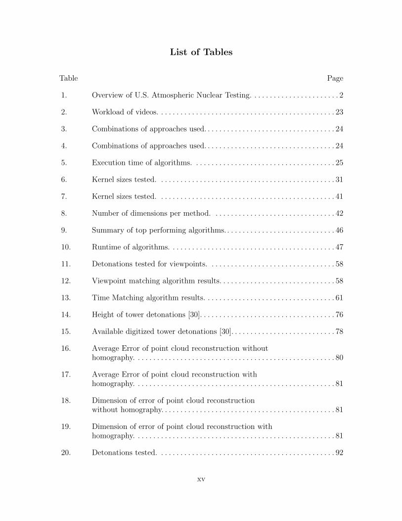
List of Tables . . . . . . . . . . . . . . . . . . . . . . . . . . . . . . . . . . . . . . . . . . . . . . . . . . . . . . . . . . . xv

I. Introduction . . . . . . . . . . . . . . . . . . . . . . . . . . . . . . . . . . . . . . . . . . . . . . . . . . . . . . . . 1

1.1 Motivation . . . . . . . . . . . . . . . . . . . . . . . . . . . . . . . . . . . . . . . . . . . . . . . . . . . . . 41.2 Hypothesis . . . . . . . . . . . . . . . . . . . . . . . . . . . . . . . . . . . . . . . . . . . . . . . . . . . . . 81.3 Research Goal . . . . . . . . . . . . . . . . . . . . . . . . . . . . . . . . . . . . . . . . . . . . . . . . . . 81.4 Challenges . . . . . . . . . . . . . . . . . . . . . . . . . . . . . . . . . . . . . . . . . . . . . . . . . . . . . . 9

Timing . . . . . . . . . . . . . . . . . . . . . . . . . . . . . . . . . . . . . . . . . . . . . . . . . . . . . . . . . 9Feature Detection . . . . . . . . . . . . . . . . . . . . . . . . . . . . . . . . . . . . . . . . . . . . . . 10Algorithm viewpoint matching limitations . . . . . . . . . . . . . . . . . . . . . . . . . 10Determining the accuracy of reconstructions . . . . . . . . . . . . . . . . . . . . . . . 12

1.5 Contributions . . . . . . . . . . . . . . . . . . . . . . . . . . . . . . . . . . . . . . . . . . . . . . . . . . 121.6 System Overview . . . . . . . . . . . . . . . . . . . . . . . . . . . . . . . . . . . . . . . . . . . . . . . 14

II. Timing Detection and Timestamp Estimation . . . . . . . . . . . . . . . . . . . . . . . . . . 16

2.1 Block diagram of NUDET Timing detector . . . . . . . . . . . . . . . . . . . . . . . . 162.2 Description of approaches . . . . . . . . . . . . . . . . . . . . . . . . . . . . . . . . . . . . . . . 17

Column Sum . . . . . . . . . . . . . . . . . . . . . . . . . . . . . . . . . . . . . . . . . . . . . . . . . . 17Circle Detection . . . . . . . . . . . . . . . . . . . . . . . . . . . . . . . . . . . . . . . . . . . . . . . . 19Change Image . . . . . . . . . . . . . . . . . . . . . . . . . . . . . . . . . . . . . . . . . . . . . . . . . 20Interval sensing and interval skipping . . . . . . . . . . . . . . . . . . . . . . . . . . . . . 21Combining approaches . . . . . . . . . . . . . . . . . . . . . . . . . . . . . . . . . . . . . . . . . . 22

2.3 Timing Results . . . . . . . . . . . . . . . . . . . . . . . . . . . . . . . . . . . . . . . . . . . . . . . . . 232.4 Time Alignment of Films . . . . . . . . . . . . . . . . . . . . . . . . . . . . . . . . . . . . . . . . 252.5 Timing Conclusions . . . . . . . . . . . . . . . . . . . . . . . . . . . . . . . . . . . . . . . . . . . . . 27

III. Subsphere Detection . . . . . . . . . . . . . . . . . . . . . . . . . . . . . . . . . . . . . . . . . . . . . . . . 29

3.1 Block diagram . . . . . . . . . . . . . . . . . . . . . . . . . . . . . . . . . . . . . . . . . . . . . . . . . 29Inputs . . . . . . . . . . . . . . . . . . . . . . . . . . . . . . . . . . . . . . . . . . . . . . . . . . . . . . . . 30Parameters . . . . . . . . . . . . . . . . . . . . . . . . . . . . . . . . . . . . . . . . . . . . . . . . . . . . 31Outputs . . . . . . . . . . . . . . . . . . . . . . . . . . . . . . . . . . . . . . . . . . . . . . . . . . . . . . . 32

3.2 Subsphere Detection Results . . . . . . . . . . . . . . . . . . . . . . . . . . . . . . . . . . . . . 32Sequential Forward Search . . . . . . . . . . . . . . . . . . . . . . . . . . . . . . . . . . . . . . . 32Principal Component Analysis Results . . . . . . . . . . . . . . . . . . . . . . . . . . . . 36

vi

Page

Best Filtering . . . . . . . . . . . . . . . . . . . . . . . . . . . . . . . . . . . . . . . . . . . . . . . . . . 363.3 Conclusions . . . . . . . . . . . . . . . . . . . . . . . . . . . . . . . . . . . . . . . . . . . . . . . . . . . . 38

IV. Hotspot Detection . . . . . . . . . . . . . . . . . . . . . . . . . . . . . . . . . . . . . . . . . . . . . . . . . . 39

4.1 Nuclear Hotspot Detector . . . . . . . . . . . . . . . . . . . . . . . . . . . . . . . . . . . . . . . 39Inputs . . . . . . . . . . . . . . . . . . . . . . . . . . . . . . . . . . . . . . . . . . . . . . . . . . . . . . . . 40Parameters . . . . . . . . . . . . . . . . . . . . . . . . . . . . . . . . . . . . . . . . . . . . . . . . . . . . 41Outputs . . . . . . . . . . . . . . . . . . . . . . . . . . . . . . . . . . . . . . . . . . . . . . . . . . . . . . . 42Dimensions . . . . . . . . . . . . . . . . . . . . . . . . . . . . . . . . . . . . . . . . . . . . . . . . . . . . 42

4.2 Hotspot Detection Results . . . . . . . . . . . . . . . . . . . . . . . . . . . . . . . . . . . . . . . 434.3 Applying Hotspot Feature Detection . . . . . . . . . . . . . . . . . . . . . . . . . . . . . . 48

V. Automated Hotspot Feature Matching . . . . . . . . . . . . . . . . . . . . . . . . . . . . . . . . 51

5.1 Methodology. . . . . . . . . . . . . . . . . . . . . . . . . . . . . . . . . . . . . . . . . . . . . . . . . . . 51Hotspot Feature Descriptor . . . . . . . . . . . . . . . . . . . . . . . . . . . . . . . . . . . . . . 52Feature Matching . . . . . . . . . . . . . . . . . . . . . . . . . . . . . . . . . . . . . . . . . . . . . . 54

5.2 Results . . . . . . . . . . . . . . . . . . . . . . . . . . . . . . . . . . . . . . . . . . . . . . . . . . . . . . . 57Matched Viewpoint Results . . . . . . . . . . . . . . . . . . . . . . . . . . . . . . . . . . . . . . 58Matched in Time Sequence Results . . . . . . . . . . . . . . . . . . . . . . . . . . . . . . . 60

5.3 Conclusion . . . . . . . . . . . . . . . . . . . . . . . . . . . . . . . . . . . . . . . . . . . . . . . . . . . . 61

VI. Quantifying Accuracy of 3D Points Clouds . . . . . . . . . . . . . . . . . . . . . . . . . . . . . 63

6.1 Background . . . . . . . . . . . . . . . . . . . . . . . . . . . . . . . . . . . . . . . . . . . . . . . . . . . 64Homogeneous coordinates . . . . . . . . . . . . . . . . . . . . . . . . . . . . . . . . . . . . . . . 65Camera Models . . . . . . . . . . . . . . . . . . . . . . . . . . . . . . . . . . . . . . . . . . . . . . . . 65Triangulation . . . . . . . . . . . . . . . . . . . . . . . . . . . . . . . . . . . . . . . . . . . . . . . . . . 70Bundle Adjustment . . . . . . . . . . . . . . . . . . . . . . . . . . . . . . . . . . . . . . . . . . . . . 732D Homography and Image Registration . . . . . . . . . . . . . . . . . . . . . . . . . . . 74

6.2 Methodology. . . . . . . . . . . . . . . . . . . . . . . . . . . . . . . . . . . . . . . . . . . . . . . . . . . 75Applying Homography . . . . . . . . . . . . . . . . . . . . . . . . . . . . . . . . . . . . . . . . . . 76Workload . . . . . . . . . . . . . . . . . . . . . . . . . . . . . . . . . . . . . . . . . . . . . . . . . . . . . 77Estimating Camera Intrinsics (K) . . . . . . . . . . . . . . . . . . . . . . . . . . . . . . . . 78

6.3 Results . . . . . . . . . . . . . . . . . . . . . . . . . . . . . . . . . . . . . . . . . . . . . . . . . . . . . . . 786.4 Discussion . . . . . . . . . . . . . . . . . . . . . . . . . . . . . . . . . . . . . . . . . . . . . . . . . . . . . 826.5 Conclusions . . . . . . . . . . . . . . . . . . . . . . . . . . . . . . . . . . . . . . . . . . . . . . . . . . . . 83

VII. Estimating Atmospheric Nuclear Detonation Volume . . . . . . . . . . . . . . . . . . . . 85

7.1 Volume Estimation Processes . . . . . . . . . . . . . . . . . . . . . . . . . . . . . . . . . . . . 85Sphere estimation from 2D image . . . . . . . . . . . . . . . . . . . . . . . . . . . . . . . . . 86Ellipsoid estimation from 2D image . . . . . . . . . . . . . . . . . . . . . . . . . . . . . . . 87Subsphere Volume estimation from 2D images . . . . . . . . . . . . . . . . . . . . . . 87Sphere from 3D point cloud . . . . . . . . . . . . . . . . . . . . . . . . . . . . . . . . . . . . . . 89

vii

Page

Ellipsoid from 3D point cloud . . . . . . . . . . . . . . . . . . . . . . . . . . . . . . . . . . . . 89Space Carving Volume . . . . . . . . . . . . . . . . . . . . . . . . . . . . . . . . . . . . . . . . . . 91Volume models using Homography . . . . . . . . . . . . . . . . . . . . . . . . . . . . . . . . 91Volume based on documented yields . . . . . . . . . . . . . . . . . . . . . . . . . . . . . . 91

7.2 Workload . . . . . . . . . . . . . . . . . . . . . . . . . . . . . . . . . . . . . . . . . . . . . . . . . . . . . 927.3 Results . . . . . . . . . . . . . . . . . . . . . . . . . . . . . . . . . . . . . . . . . . . . . . . . . . . . . . . 937.4 Conclusions . . . . . . . . . . . . . . . . . . . . . . . . . . . . . . . . . . . . . . . . . . . . . . . . . . . . 96

VIII. Conclusion and Future Work . . . . . . . . . . . . . . . . . . . . . . . . . . . . . . . . . . . . . . . . . 99

8.1 Contributions . . . . . . . . . . . . . . . . . . . . . . . . . . . . . . . . . . . . . . . . . . . . . . . . . . 998.2 Future Work . . . . . . . . . . . . . . . . . . . . . . . . . . . . . . . . . . . . . . . . . . . . . . . . . . 101

Appendix A. Camera Calibration . . . . . . . . . . . . . . . . . . . . . . . . . . . . . . . . . . . . . . . . 103

1.1 Estimating Camera Intrinsics (K) . . . . . . . . . . . . . . . . . . . . . . . . . . . . . . . 103Estimating mx and my . . . . . . . . . . . . . . . . . . . . . . . . . . . . . . . . . . . . . . . . . 103Estimating x0 and y0 . . . . . . . . . . . . . . . . . . . . . . . . . . . . . . . . . . . . . . . . . . 106Estimating (K) . . . . . . . . . . . . . . . . . . . . . . . . . . . . . . . . . . . . . . . . . . . . . . . 108

1.2 Estimating P . . . . . . . . . . . . . . . . . . . . . . . . . . . . . . . . . . . . . . . . . . . . . . . . . 1091.3 Conclusion . . . . . . . . . . . . . . . . . . . . . . . . . . . . . . . . . . . . . . . . . . . . . . . . . . . 111

Bibliography . . . . . . . . . . . . . . . . . . . . . . . . . . . . . . . . . . . . . . . . . . . . . . . . . . . . . . . . . . 112

viii

List of Figures

Figure Page

1. An example of survey data collected for Tesla [30]. . . . . . . . . . . . . . . . . . . . 3

2. Map of Tesla explosion [30]. The red circle is thedetonation site and the blue triangles are film collectionsites. . . . . . . . . . . . . . . . . . . . . . . . . . . . . . . . . . . . . . . . . . . . . . . . . . . . . . . . . . . . 4

3. A typical arrangement of cameras within a collectionsite [30]. . . . . . . . . . . . . . . . . . . . . . . . . . . . . . . . . . . . . . . . . . . . . . . . . . . . . . . . . 5

4. On left is the Eastman High Speed Camera. On right isthe Fastax camera [32]. . . . . . . . . . . . . . . . . . . . . . . . . . . . . . . . . . . . . . . . . . . . 5

5. The operation of a rotating prism camera [32]. . . . . . . . . . . . . . . . . . . . . . . . 6

6. An example timing mark. . . . . . . . . . . . . . . . . . . . . . . . . . . . . . . . . . . . . . . . . . 7

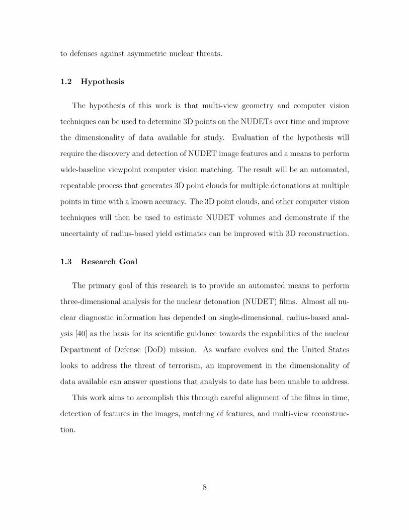
7. The Goldeneye scanner that is used by LLNL to digitizethe NUDET films [30]. . . . . . . . . . . . . . . . . . . . . . . . . . . . . . . . . . . . . . . . . . . . 7

8. Tesla explosion [30] with two subspheres identified. . . . . . . . . . . . . . . . . . . 11

9. Grable nuclear detonation [30] with some “hotspots”identified. Also identified is a timing mark used tomeasure time in the variable high-speed cameras. . . . . . . . . . . . . . . . . . . . 12

10. An flow diagram of processing NUDET images intovolume estimation. . . . . . . . . . . . . . . . . . . . . . . . . . . . . . . . . . . . . . . . . . . . . . . 15

11. NUDET Timing detector Block Diagram. . . . . . . . . . . . . . . . . . . . . . . . . . . 17

12. A cubic spline fit to the frame rate of the Climaxdetonation. . . . . . . . . . . . . . . . . . . . . . . . . . . . . . . . . . . . . . . . . . . . . . . . . . . . . 25

13. The methodology to align the timing of films with timet = 0 [31]. . . . . . . . . . . . . . . . . . . . . . . . . . . . . . . . . . . . . . . . . . . . . . . . . . . . . . 27

14. A plot of radius growth over time based on timeestimates from multiple cameras from Tesla Truck 7. Afew outliers exist that were a result of errors in theautomated detection of the radius of the detonation. . . . . . . . . . . . . . . . . 28

15. Block Diagram for Subsphere Detector. . . . . . . . . . . . . . . . . . . . . . . . . . . . . 30

ix

Figure Page

16. ROC curve for SFS 15×15, no filter. Each point islabeled with the number of dimensions representing theTop N dimensions that were used. . . . . . . . . . . . . . . . . . . . . . . . . . . . . . . . . 33

17. Image representation of detections for SFS 15×15, 18dimensions, no filter. Areas in light blue are falsedetections. Each subsphere is traced in red.Overlapping light blue with red represents a truepositive. . . . . . . . . . . . . . . . . . . . . . . . . . . . . . . . . . . . . . . . . . . . . . . . . . . . . . . 34

18. Image representation of detections for SFS 15×15, 18dimensions, with a post-process 4×4 averaging filter.Areas in orange are false detections. Areas in red aretrue positives. . . . . . . . . . . . . . . . . . . . . . . . . . . . . . . . . . . . . . . . . . . . . . . . . . . 34

19. ROC curve for SFS 15×15, Weiner filter. Each point islabeled with the number of dimensions representing theTop N dimensions that were used. . . . . . . . . . . . . . . . . . . . . . . . . . . . . . . . . 35

20. ROC curve for SFS 15×15, Median filter. Each point islabeled with the number of dimensions representing theTop N dimensions that were used. . . . . . . . . . . . . . . . . . . . . . . . . . . . . . . . . 35

21. ROC curve for PCA 21×21, no filter. Each point islabeled with the number of dimensions representing theTop N dimensions that were used. . . . . . . . . . . . . . . . . . . . . . . . . . . . . . . . . 36

22. Image representation of detections for PCA 21×21, nofilter. Areas in light blue are false detections. Eachsubsphere is traced in red. Overlapping light blue withred represents true positive detections. . . . . . . . . . . . . . . . . . . . . . . . . . . . . . 37

23. Image representation of detections for PCA 21×21, witha post-process 4×4 averaging filter. Areas in orange arefalse detections. Areas in red are true positives. . . . . . . . . . . . . . . . . . . . . . 37

24. Block Diagram for Hotspot Detector . . . . . . . . . . . . . . . . . . . . . . . . . . . . . . 40

x

Figure Page

25. Four examples of sub-kernel schemes. The 5×5 gridrepresents 25 sub-kernels for a 25×25 or 15×15 kernel.In the 25×25 case, each square represents a 5×5 pixelarea, while in the 15×15 case each square is a 3×3 pixelarea. An averaging dimension value example would be,averaging the green pixels and subtracted them from anaverage of the blue pixels. A min/max dimensionexample would take an average of the max of the greensub-kernels minus an average of the min of the blue pixels. . . . . . . . . . . . 43

26. Hit rate by dimension reduction algorithm and numberof dimensions. In general, the SFS algorithmsperformed best, with PCA algorithms improving ascomponents were added. . . . . . . . . . . . . . . . . . . . . . . . . . . . . . . . . . . . . . . . . . 44

27. Precision by dimension reduction algorithm and numberof dimensions. . . . . . . . . . . . . . . . . . . . . . . . . . . . . . . . . . . . . . . . . . . . . . . . . . . 44

28. False alarm rate by dimension reduction algorithm andnumber of dimensions. . . . . . . . . . . . . . . . . . . . . . . . . . . . . . . . . . . . . . . . . . . . 45

29. A comparison of truth clustering effects on the results ofSFS 25×25. Red represents pixels that are truepositives. Light green are pixels that are false positives.Without clustering, the left figure has true positives(red dots) surrounded by false positives that iscorrected in the right figure. . . . . . . . . . . . . . . . . . . . . . . . . . . . . . . . . . . . . . 46

30. Results of detections for ReliefF, 25×25 kernel, top 3dimensions plotted on an image. Red represents pixelsthat are true positives (visible inside the light greenband). Light green are pixels that are false positives.Clustering turns all the false positives into one largetrue positive around the exterior of the explosion, andmisses true positives in the center of the explosion. . . . . . . . . . . . . . . . . . . 47

31. A comparison of truth clustering effects on the results ofPCA 25×25 kernel with histogram equalization. Theleft image is 12 dimensions and the right image is 24dimensions. Red represents pixels that are truepositives. Light green are pixels that are false positives. . . . . . . . . . . . . . 48

xi

Figure Page

32. Results of hotspot detector for Boltzmann detonation.There were 141 true positive detections, 20 misses, and15 false detections(1,67,83,111,120,127,129,130,136,141,146,151,154,155and 156). Boundary of the detonation is highlighted inblue is the result of ellipse detection [39]. . . . . . . . . . . . . . . . . . . . . . . . . . . 50

33. A flow chart of step-by-step processes resulting inhotspot feature correspondences from differentviewpoints and points in time. . . . . . . . . . . . . . . . . . . . . . . . . . . . . . . . . . . . . 52

34. A depiction of 3-dimensional polar coordinates.Inclination angle from the vertical axis is θ. Azimuthangle from the depth axis(X-axis) is ϕ. The radius inthe direction of θ and ϕ is r. . . . . . . . . . . . . . . . . . . . . . . . . . . . . . . . . . . . . . 54

35. Results of viewpoint matching for hotspots are x’s inthe Grable detonation. There were 68 correct matches,and 3 incorrect matches (2, 28, 61). SURF matches areshown with lines with none of them being correct. . . . . . . . . . . . . . . . . . . . 59

36. Results of time sequence matching for hotspots in theTurk detonation. The numbered x’s are the hotspotmatching results and the corresponding lines are SIFTmatches. All matches for the hotspot matching werecorrect, while the SIFT matching has two mismatchesand eighteen correct matches. . . . . . . . . . . . . . . . . . . . . . . . . . . . . . . . . . . . . 60

37. An example NUDET image of Tesla detonation withtower visible below the detonation [30]. . . . . . . . . . . . . . . . . . . . . . . . . . . . . 64

38. The pinhole camera model. . . . . . . . . . . . . . . . . . . . . . . . . . . . . . . . . . . . . . . 66

39. The Euclidean transformation between world andcamera coordinate frames is comprised of rotation (R)and translation (t) [8]. . . . . . . . . . . . . . . . . . . . . . . . . . . . . . . . . . . . . . . . . . . 68

40. 3D point triangulation [34]. Point p is estimated usingrays traced from the centers of camera at R1c1 and R2c2. . . . . . . . . . . . . 71

xii

Figure Page

41. Applying homography to register images prior topairwise comparison. Each point of view uses SURFderived correspondences to calculate H. The manualpoints are then transformed to one coordinate systemand averaged. The average is then transformed backinto the original coordinate systems and are thencompared pairwise and measured with triangulation andbundle adjustment with the alternate point of view. . . . . . . . . . . . . . . . . . 77

42. Matched correspondences of Film 04 with Film 10 ofTesla. . . . . . . . . . . . . . . . . . . . . . . . . . . . . . . . . . . . . . . . . . . . . . . . . . . . . . . . . . 79

43. 3D Reconstruction of Film 04 with Film 10 of Tesla. . . . . . . . . . . . . . . . . 79

44. Flow diagram of estimating the radius of an explosion. . . . . . . . . . . . . . . . 86

45. Flow diagram of estimating the subsphere location. . . . . . . . . . . . . . . . . . . 89

46. Hotspot detection and matching [25] results on Climaxdetonation. . . . . . . . . . . . . . . . . . . . . . . . . . . . . . . . . . . . . . . . . . . . . . . . . . . . . 90

47. 3D point cloud and least squares sphere fit to Tesladetonation hotspots. . . . . . . . . . . . . . . . . . . . . . . . . . . . . . . . . . . . . . . . . . . . . 90

48. Rendering of space carving results from two cameras ofthe MET detonation. . . . . . . . . . . . . . . . . . . . . . . . . . . . . . . . . . . . . . . . . . . . . 92

49. Volume estimates of Climax. . . . . . . . . . . . . . . . . . . . . . . . . . . . . . . . . . . . . . 96

50. Volume estimates of Grable. . . . . . . . . . . . . . . . . . . . . . . . . . . . . . . . . . . . . . . 97

51. Volume estimates of Tesla. . . . . . . . . . . . . . . . . . . . . . . . . . . . . . . . . . . . . . . . 98

52. Volume estimates of MET. . . . . . . . . . . . . . . . . . . . . . . . . . . . . . . . . . . . . . . . 98

53. Dimensions of the 16mm film[30]. . . . . . . . . . . . . . . . . . . . . . . . . . . . . . . . . 105

54. A pictorial example of different principal points. Theboundaries of different methods are outlined with theircenter principal point. Green is based on the overallimage, Blue is based on the viewable area, Red is basedon the emulsion layer reacting with the light. . . . . . . . . . . . . . . . . . . . . . . 108

xiii

Figure Page

55. A summary of pixel intensities by column. The lowpoints on either side represent where the best area tocrop the images would be. . . . . . . . . . . . . . . . . . . . . . . . . . . . . . . . . . . . . . . 109

56. An example of survey data collected for Tesla [30]. . . . . . . . . . . . . . . . . . 111

xiv

List of Tables

Table Page

1. Overview of U.S. Atmospheric Nuclear Testing. . . . . . . . . . . . . . . . . . . . . . . 2

2. Workload of videos. . . . . . . . . . . . . . . . . . . . . . . . . . . . . . . . . . . . . . . . . . . . . . 23

3. Combinations of approaches used. . . . . . . . . . . . . . . . . . . . . . . . . . . . . . . . . . 24

4. Combinations of approaches used. . . . . . . . . . . . . . . . . . . . . . . . . . . . . . . . . . 24

5. Execution time of algorithms. . . . . . . . . . . . . . . . . . . . . . . . . . . . . . . . . . . . . 25

6. Kernel sizes tested. . . . . . . . . . . . . . . . . . . . . . . . . . . . . . . . . . . . . . . . . . . . . . 31

7. Kernel sizes tested. . . . . . . . . . . . . . . . . . . . . . . . . . . . . . . . . . . . . . . . . . . . . . 41

8. Number of dimensions per method. . . . . . . . . . . . . . . . . . . . . . . . . . . . . . . . 42

9. Summary of top performing algorithms. . . . . . . . . . . . . . . . . . . . . . . . . . . . . 46

10. Runtime of algorithms. . . . . . . . . . . . . . . . . . . . . . . . . . . . . . . . . . . . . . . . . . . 47

11. Detonations tested for viewpoints. . . . . . . . . . . . . . . . . . . . . . . . . . . . . . . . . 58

12. Viewpoint matching algorithm results. . . . . . . . . . . . . . . . . . . . . . . . . . . . . . 58

13. Time Matching algorithm results. . . . . . . . . . . . . . . . . . . . . . . . . . . . . . . . . . 61

14. Height of tower detonations [30]. . . . . . . . . . . . . . . . . . . . . . . . . . . . . . . . . . . 76

15. Available digitized tower detonations [30]. . . . . . . . . . . . . . . . . . . . . . . . . . . 78

16. Average Error of point cloud reconstruction withouthomography. . . . . . . . . . . . . . . . . . . . . . . . . . . . . . . . . . . . . . . . . . . . . . . . . . . . 80

17. Average Error of point cloud reconstruction withhomography. . . . . . . . . . . . . . . . . . . . . . . . . . . . . . . . . . . . . . . . . . . . . . . . . . . . 81

18. Dimension of error of point cloud reconstructionwithout homography. . . . . . . . . . . . . . . . . . . . . . . . . . . . . . . . . . . . . . . . . . . . . 81

19. Dimension of error of point cloud reconstruction withhomography. . . . . . . . . . . . . . . . . . . . . . . . . . . . . . . . . . . . . . . . . . . . . . . . . . . . 81

20. Detonations tested. . . . . . . . . . . . . . . . . . . . . . . . . . . . . . . . . . . . . . . . . . . . . . 92

xv

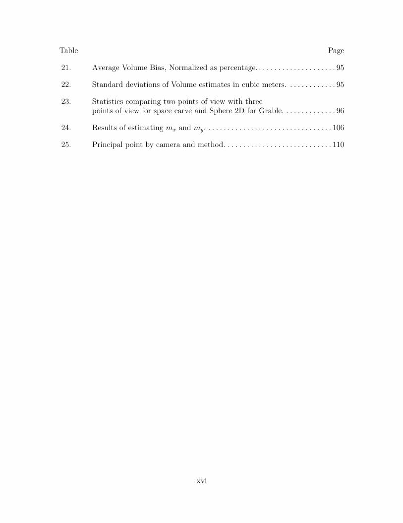
Table Page

21. Average Volume Bias, Normalized as percentage. . . . . . . . . . . . . . . . . . . . . 95

22. Standard deviations of Volume estimates in cubic meters. . . . . . . . . . . . . 95

23. Statistics comparing two points of view with threepoints of view for space carve and Sphere 2D for Grable. . . . . . . . . . . . . . 96

24. Results of estimating mx and my. . . . . . . . . . . . . . . . . . . . . . . . . . . . . . . . . 106

25. Principal point by camera and method. . . . . . . . . . . . . . . . . . . . . . . . . . . . 110

xvi



I. Introduction

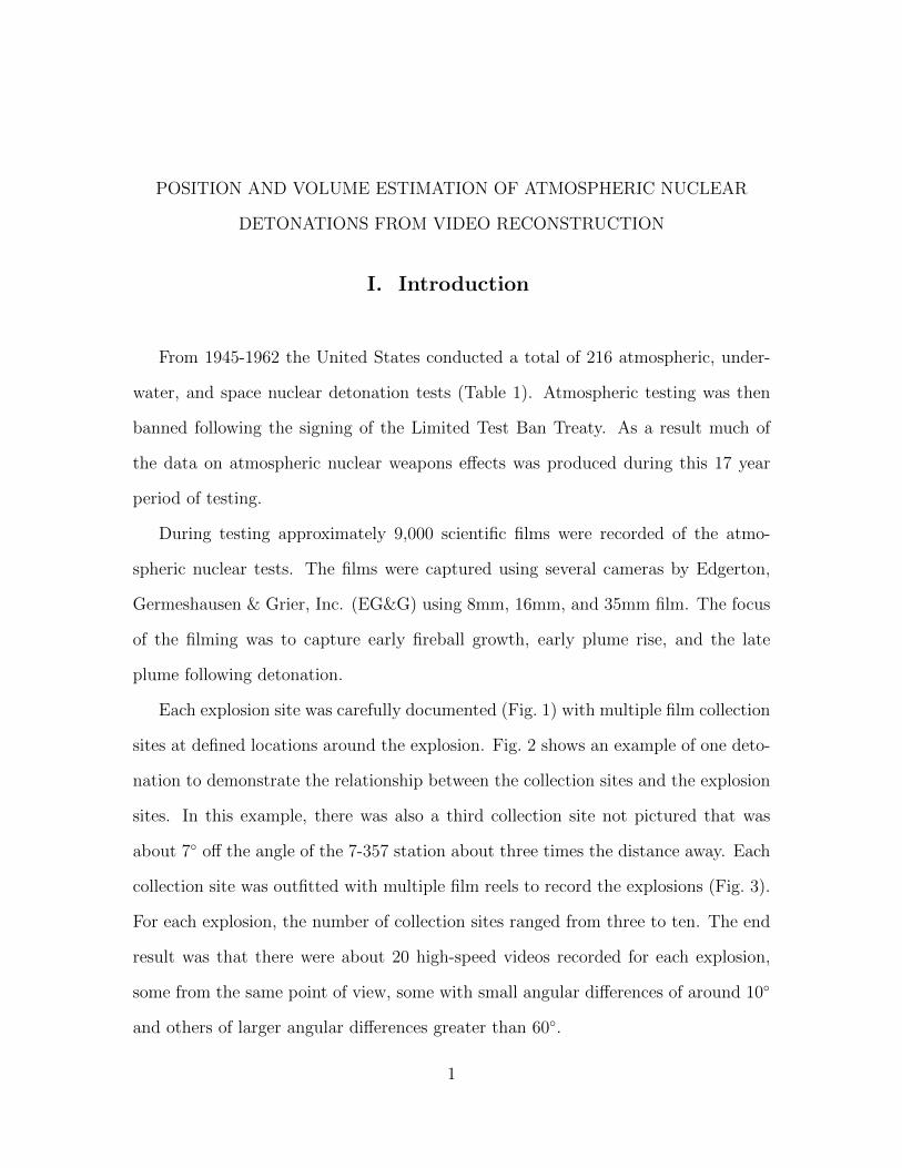
From 1945-1962 the United States conducted a total of 216 atmospheric, under-

water, and space nuclear detonation tests (Table 1). Atmospheric testing was then

banned following the signing of the Limited Test Ban Treaty. As a result much of

the data on atmospheric nuclear weapons effects was produced during this 17 year

period of testing.

During testing approximately 9,000 scientific films were recorded of the atmo-

spheric nuclear tests. The films were captured using several cameras by Edgerton,

Germeshausen & Grier, Inc. (EG&G) using 8mm, 16mm, and 35mm film. The focus

of the filming was to capture early fireball growth, early plume rise, and the late

plume following detonation.

Each explosion site was carefully documented (Fig. 1) with multiple film collection

sites at defined locations around the explosion. Fig. 2 shows an example of one deto-

nation to demonstrate the relationship between the collection sites and the explosion

sites. In this example, there was also a third collection site not pictured that was

about 7◦ off the angle of the 7-357 station about three times the distance away. Each

collection site was outfitted with multiple film reels to record the explosions (Fig. 3).

For each explosion, the number of collection sites ranged from three to ten. The end

result was that there were about 20 high-speed videos recorded for each explosion,

some from the same point of view, some with small angular differences of around 10◦

and others of larger angular differences greater than 60◦.

1

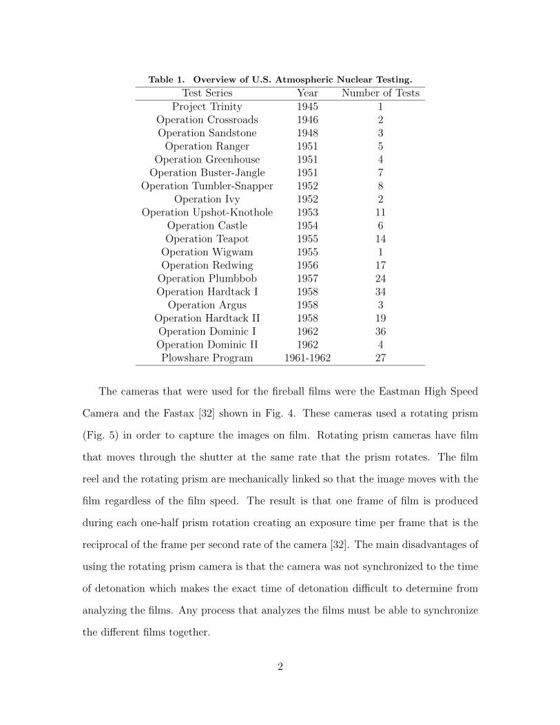
Table 1. Overview of U.S. Atmospheric Nuclear Testing.

Test Series Year Number of TestsProject Trinity 1945 1

Operation Crossroads 1946 2Operation Sandstone 1948 3

Operation Ranger 1951 5Operation Greenhouse 1951 4

Operation Buster-Jangle 1951 7Operation Tumbler-Snapper 1952 8

Operation Ivy 1952 2Operation Upshot-Knothole 1953 11

Operation Castle 1954 6Operation Teapot 1955 14

Operation Wigwam 1955 1Operation Redwing 1956 17

Operation Plumbbob 1957 24Operation Hardtack I 1958 34

Operation Argus 1958 3Operation Hardtack II 1958 19Operation Dominic I 1962 36Operation Dominic II 1962 4Plowshare Program 1961-1962 27

The cameras that were used for the fireball films were the Eastman High Speed

Camera and the Fastax [32] shown in Fig. 4. These cameras used a rotating prism

(Fig. 5) in order to capture the images on film. Rotating prism cameras have film

that moves through the shutter at the same rate that the prism rotates. The film

reel and the rotating prism are mechanically linked so that the image moves with the

film regardless of the film speed. The result is that one frame of film is produced

during each one-half prism rotation creating an exposure time per frame that is the

reciprocal of the frame per second rate of the camera [32]. The main disadvantages of

using the rotating prism camera is that the camera was not synchronized to the time

of detonation which makes the exact time of detonation difficult to determine from

analyzing the films. Any process that analyzes the films must be able to synchronize

the different films together.

2

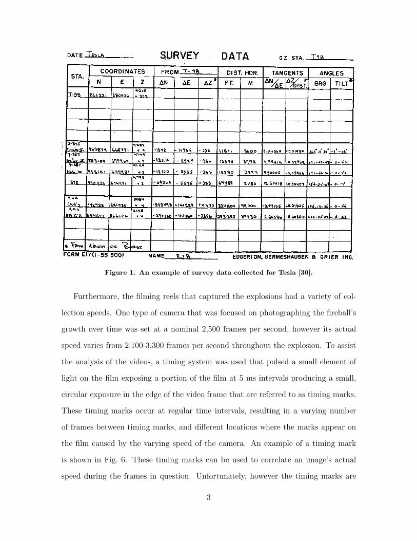
Figure 1. An example of survey data collected for Tesla [30].

Furthermore, the filming reels that captured the explosions had a variety of col-

lection speeds. One type of camera that was focused on photographing the fireball’s

growth over time was set at a nominal 2,500 frames per second, however its actual

speed varies from 2,100-3,300 frames per second throughout the explosion. To assist

the analysis of the videos, a timing system was used that pulsed a small element of

light on the film exposing a portion of the film at 5 ms intervals producing a small,

circular exposure in the edge of the video frame that are referred to as timing marks.

These timing marks occur at regular time intervals, resulting in a varying number

of frames between timing marks, and different locations where the marks appear on

the film caused by the varying speed of the camera. An example of a timing mark

is shown in Fig. 6. These timing marks can be used to correlate an image’s actual

speed during the frames in question. Unfortunately, however the timing marks are

3

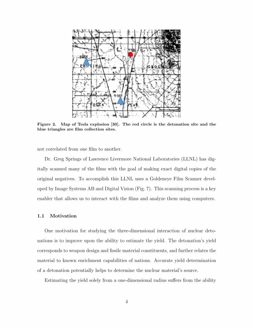
Figure 2. Map of Tesla explosion [30]. The red circle is the detonation site and theblue triangles are film collection sites.

not correlated from one film to another.

Dr. Greg Springs of Lawrence Livermore National Laboratories (LLNL) has dig-

itally scanned many of the films with the goal of making exact digital copies of the

original negatives. To accomplish this LLNL uses a Goldeneye Film Scanner devel-

oped by Image Systems AB and Digital Vision (Fig. 7). This scanning process is a key

enabler that allows us to interact with the films and analyze them using computers.

1.1 Motivation

One motivation for studying the three-dimensional interaction of nuclear deto-

nations is to improve upon the ability to estimate the yield. The detonation’s yield

corresponds to weapon design and fissile material constituents, and further relates the

material to known enrichment capabilities of nations. Accurate yield determination

of a detonation potentially helps to determine the nuclear material’s source.

Estimating the yield solely from a one-dimensional radius suffers from the ability

4

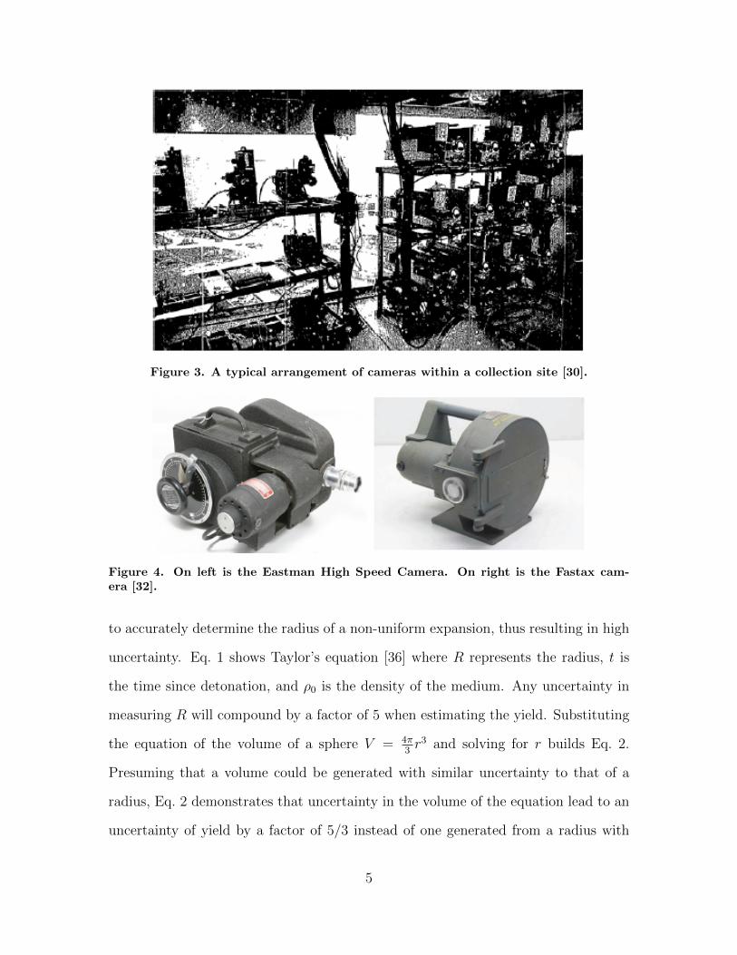
Figure 3. A typical arrangement of cameras within a collection site [30].

Figure 4. On left is the Eastman High Speed Camera. On right is the Fastax cam-era [32].

to accurately determine the radius of a non-uniform expansion, thus resulting in high

uncertainty. Eq. 1 shows Taylor’s equation [36] where R represents the radius, t is

the time since detonation, and ρ0 is the density of the medium. Any uncertainty in

measuring R will compound by a factor of 5 when estimating the yield. Substituting

the equation of the volume of a sphere V = 4π3r3 and solving for r builds Eq. 2.

Presuming that a volume could be generated with similar uncertainty to that of a

radius, Eq. 2 demonstrates that uncertainty in the volume of the equation lead to an

uncertainty of yield by a factor of 5/3 instead of one generated from a radius with

5

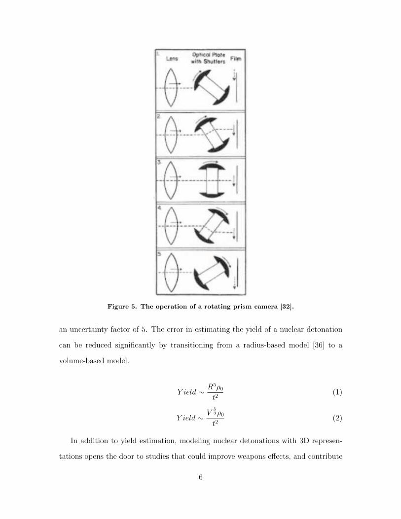
Figure 5. The operation of a rotating prism camera [32].

an uncertainty factor of 5. The error in estimating the yield of a nuclear detonation

can be reduced significantly by transitioning from a radius-based model [36] to a

volume-based model.

Y ield ∼ R5ρ0

t2(1)

Y ield ∼ V53ρ0

t2(2)

In addition to yield estimation, modeling nuclear detonations with 3D represen-

tations opens the door to studies that could improve weapons effects, and contribute

6

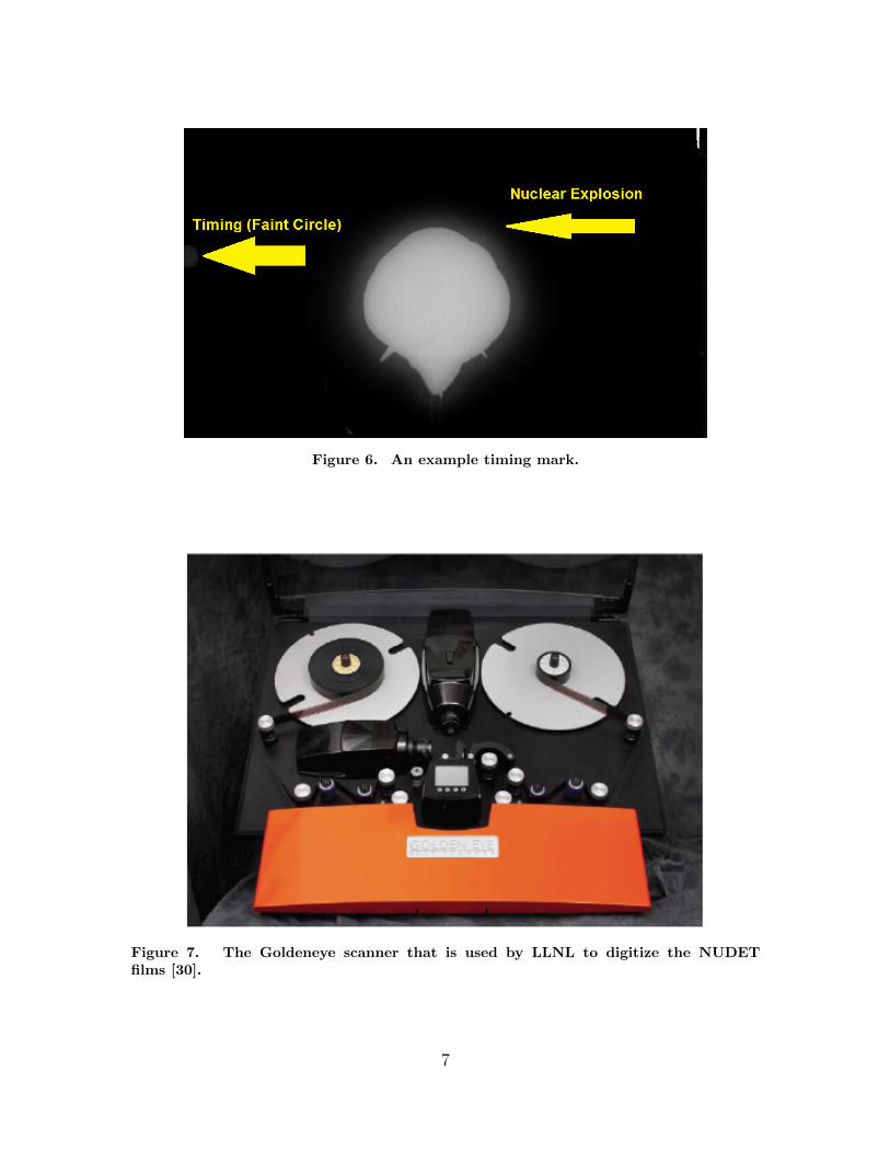
Figure 6. An example timing mark.

Figure 7. The Goldeneye scanner that is used by LLNL to digitize the NUDETfilms [30].

7

to defenses against asymmetric nuclear threats.

1.2 Hypothesis

The hypothesis of this work is that multi-view geometry and computer vision

techniques can be used to determine 3D points on the NUDETs over time and improve

the dimensionality of data available for study. Evaluation of the hypothesis will

require the discovery and detection of NUDET image features and a means to perform

wide-baseline viewpoint computer vision matching. The result will be an automated,

repeatable process that generates 3D point clouds for multiple detonations at multiple

points in time with a known accuracy. The 3D point clouds, and other computer vision

techniques will then be used to estimate NUDET volumes and demonstrate if the

uncertainty of radius-based yield estimates can be improved with 3D reconstruction.

1.3 Research Goal

The primary goal of this research is to provide an automated means to perform

three-dimensional analysis for the nuclear detonation (NUDET) films. Almost all nu-

clear diagnostic information has depended on single-dimensional, radius-based anal-

ysis [40] as the basis for its scientific guidance towards the capabilities of the nuclear

Department of Defense (DoD) mission. As warfare evolves and the United States

looks to address the threat of terrorism, an improvement in the dimensionality of

data available can answer questions that analysis to date has been unable to address.

This work aims to accomplish this through careful alignment of the films in time,

detection of features in the images, matching of features, and multi-view reconstruc-

tion.

8

1.4 Challenges

There are several challenges to creating a three-dimensional reconstruction of a

nuclear detonation. There are challenges in timing, detecting features, matching

features, and determining the accuracy of 3D reconstructions. Each of these are

discussed in turn.

Timing.

The films have uncertainty with regard to timing as a result of the mechanical

nature of the cameras. While the time between timing marks is consistent at 5 msec,

each frame is recorded every 0.25 - 0.5 msec. The resulting gaps of 10-15 frames

between timing marks leave room for error than is not measurable. Analyzing the

changing speed of the camera enables the determination of how the speed of the

camera changes over several timing marks, but is unable to determine what happens

between timing marks. This means that frame-to-frame there are potential timing

inaccuracies relating to the mechanical cameras that cannot be modeled perfectly.

These timing inconsistencies compound when frames from multiple films are com-

pared. Ideally, for three-dimensional reconstructions to be accurate, they need to be

derived from frames at exactly the same time, or the error in time will translate into

a positional error.

To create a three-dimensional reconstruction requires at least two points of view

of the object at the same point in time. Unfortunately, in the case of the NUDET

domain, the object’s shape is changing rapidly, and the timing is not accurate enough

to align multiple films together. Furthermore, with the relative speeds of cameras

being different, frames within a film fall in and out of time alignment when compared

one to another. The end result is that some frame-to-frame comparisons across view-

points are better than others with respect to time alignment. The process to address

9

these timing challenges is discussed in Chapter II.

Feature Detection.

Another challenge with the films is the detection of features that could be corre-

lated across films and used either for 3D reconstruction or volume estimation. There

are variations of the manner of which films reacted to the detonations causing a va-

riety of brightness and contrast from film to film. Also, within a given film, the light

level changes as the detonation develops. Despite these lighting changes, the naked

eye can detect areas of interest that can be correlated across viewpoints. Two features

are notable by the naked eye that will be referred to as ‘subspheres’ and ‘hotspots.’

Subspheres (Fig. 8) are features that are present in detonations that have obstruc-

tions that interact with the shockwave of the detonation. Improvements in volume

estimation could be achieved by detecting and estimating the size of these larger

deformities. Chapter III discusses the automated detection of subsphere features.

Hotspots are features that are visible in most detonations during a stage in the

detonation when the light emitted by the fireball is relatively low. Shown in Fig. 9,

they exist all over the outside boundary of the detonation and are visible from dif-

ferent viewpoints. Hotspot features have the potential to be matched from alternate

viewpoints in order to enable 3D reconstruction. The detection of hotspots is dis-

cussed in Chapter IV.

Algorithm viewpoint matching limitations.

Another challenge is that the best feature descriptors and algorithms are limited on

how repeatable their matching algorithms are from wide viewpoints. For example, one

popular multi-view geometry (MVG) method uses Scale-Invariant Feature Transform

(SIFT) [15] feature detection and matching [29]. These algorithms perform well when

10

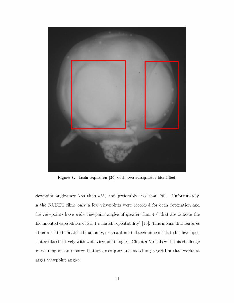
Figure 8. Tesla explosion [30] with two subspheres identified.

viewpoint angles are less than 45◦, and preferably less than 20◦. Unfortunately,

in the NUDET films only a few viewpoints were recorded for each detonation and

the viewpoints have wide viewpoint angles of greater than 45◦ that are outside the

documented capabilities of SIFT’s match repeatability) [15]. This means that features

either need to be matched manually, or an automated technique needs to be developed

that works effectively with wide viewpoint angles. Chapter V deals with this challenge

by defining an automated feature descriptor and matching algorithm that works at

larger viewpoint angles.

11

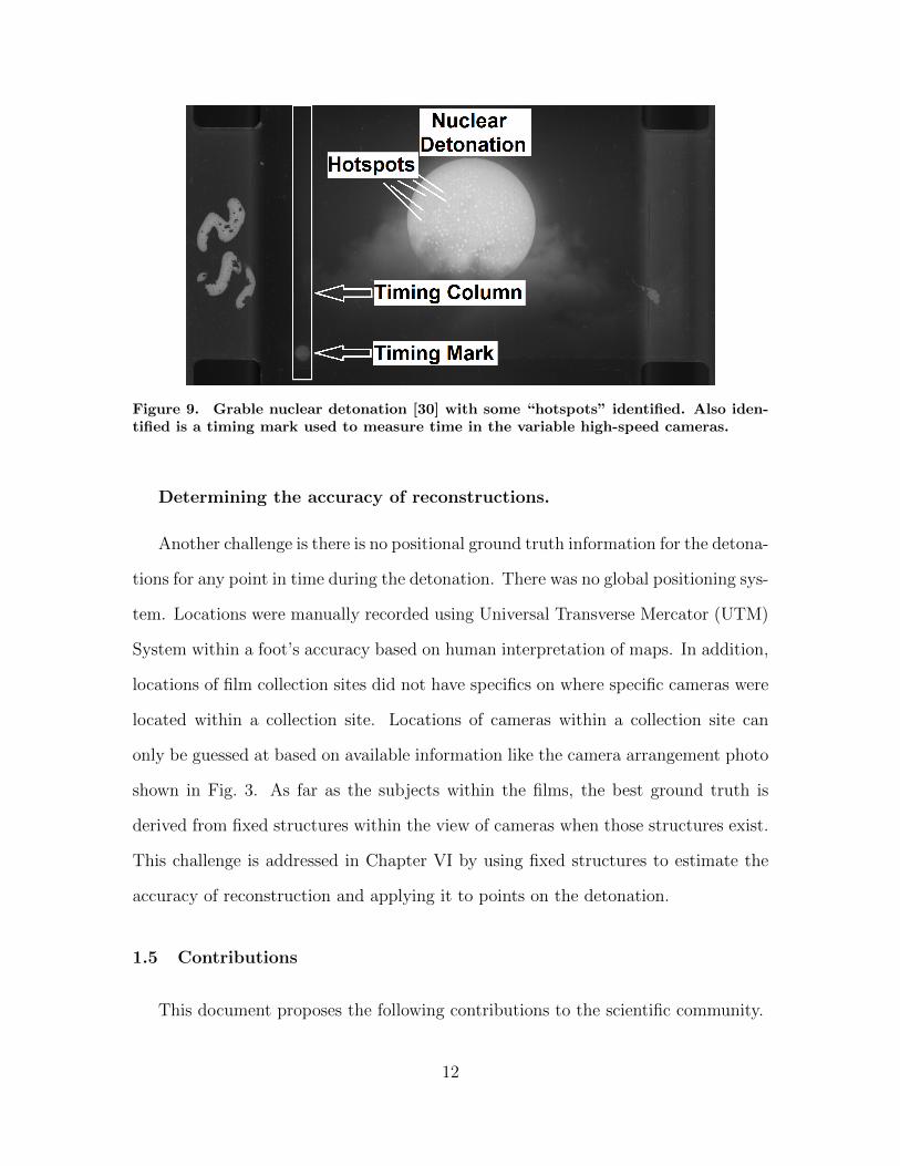
Figure 9. Grable nuclear detonation [30] with some “hotspots” identified. Also iden-tified is a timing mark used to measure time in the variable high-speed cameras.

Determining the accuracy of reconstructions.

Another challenge is there is no positional ground truth information for the detona-

tions for any point in time during the detonation. There was no global positioning sys-

tem. Locations were manually recorded using Universal Transverse Mercator (UTM)

System within a foot’s accuracy based on human interpretation of maps. In addition,

locations of film collection sites did not have specifics on where specific cameras were

located within a collection site. Locations of cameras within a collection site can

only be guessed at based on available information like the camera arrangement photo

shown in Fig. 3. As far as the subjects within the films, the best ground truth is

derived from fixed structures within the view of cameras when those structures exist.

This challenge is addressed in Chapter VI by using fixed structures to estimate the

accuracy of reconstruction and applying it to points on the detonation.

1.5 Contributions

This document proposes the following contributions to the scientific community.

12

• The production of 3D sparse point clouds to track and study features of deto-

nations over time.

• An automated process to detect and match hotspot features across wide view-

points.

The novelty of the first contribution is that there are currently no scale 3D recon-

structions of NUDETs. Understanding the second contribution, hotspot matching,

requires some background on the state-of-the-art computer vision techniques.

Scale 3D reconstructions require either calibrated cameras as in the case with

multi-view stereo (MVS) [27] or require matched correspondences on features between

multiple viewpoints to generate 3D point clouds. The NUDET films do not provide

camera calibration models, thus making direct use of MVS unreliable. Hence, novel

methods will be required to successfully evaluate this problem domain.

SIFT [15] feature matching ,and likewise Speeded-Up Robust Features (SURF) [2],

have been used for uncalibrated images [29] however, it has challenges for feature

matching with the NUDET films. Only a few viewpoints were recorded for each

detonation and the viewpoints have wide viewpoint angles ranging from 58◦ to 110◦,

which are outside the documented capabilities of SIFT’s viewpoint match repeata-

bility [15]. Methods such as Affine-Invariant SIFT (ASIFT) [18] that extend the

viewpoint angles for SIFT up to 90◦ exist, but ASIFT requires planar surfaces with

detectable Harris corners [7] that do not exist in the NUDET films, thus making

the algorithm inappropriate for this domain. Manual matching is a viable option

and is demonstrated in Chapter VI, but it is cumbersome for such an extensive data

set. Because of these issues, a feature descriptor and matching algorithm capable of

matching features with wide viewpoint angles (i.e 58◦ to 110◦) without the use of

Harris corners is a contribution not only to the physics community, but the computer

vision community as well.

13

1.6 System Overview

The overall goal is to create a reliable and repeatable process to generate 3D

point clouds of NUDET features and use those features as a basis for volumetric

reconstructionss of detonations using the films. Fig. 10 shows a flow of the information

as it is processed from images to 3D reconstruction and volume estimation. The

process begins at the left with a sequence of images for each camera. Using the

sequence and timing mark detection (Chapter II) images are tagged with the time and

possible timing error. They are organized and matched by point of view identifying

complete sets of cameras that cover all possible points of view that are also best

aligned in time. Because each camera film speed is different and changes over time,

there are periods that the time overlap is better than others. Once images are time

aligned, subsphere (Chapter III) and hotspot features (Chapter IV) are detected.

Hotspot features are used to create correspondence matches between images that

form the basis for 3D reconstruction (Chapter V). Accuracy of approximation can

be determined by the method used to generate the 3D reconstruction (Chapter VI).

Lastly, the subspheres and 3D sparse point clouds can be used to estimate the volume

of the detonation (Chapter VII).

14

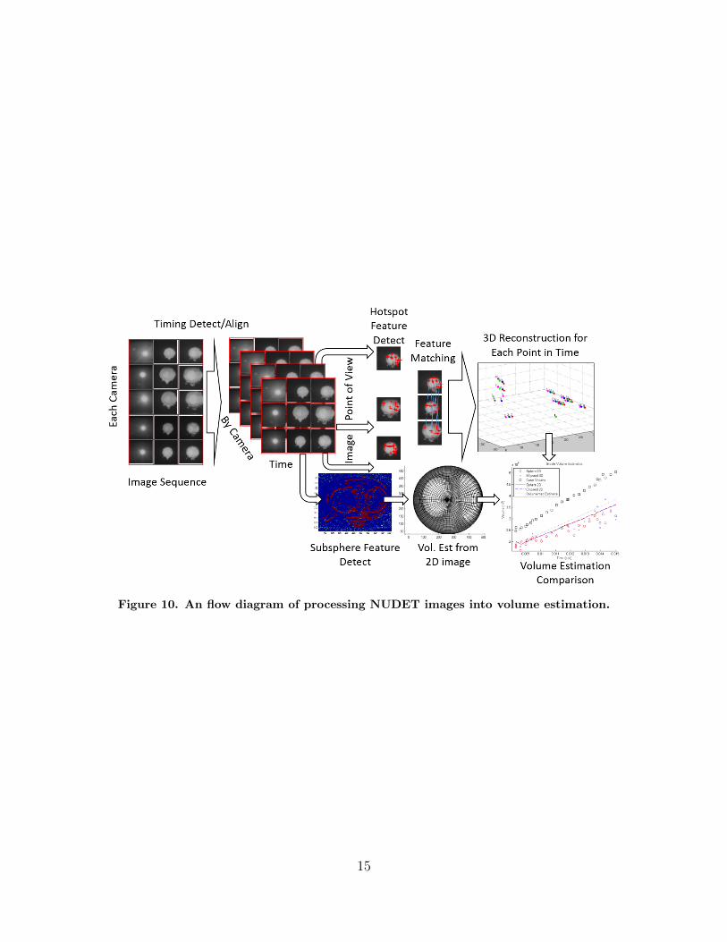
Figure 10. An flow diagram of processing NUDET images into volume estimation.

15

II. Timing Detection and Timestamp Estimation

Processing images toward 3D reconstruction requires images that have been cap-

tured close in time or of a static environment [8]. It is essential that timing is done

correctly so that the images can be compared at the same points in time. If im-

ages were compared at different points in time, results would induce unrealistic and

inaccurate reconstructions.

Timing detection begins with a sequence of images that are known to have timing

marks as shown in Fig. 6. With the knowledge that each timing mark is 5 msec apart,

the timing marks can be automatically detected in the images and their location

within the films can be modeled mathematically to determine their time relative to

the start of the detonation. This material appears in the Institute of Electrical and

Electronics Engineers (IEEE) Computer Society’s Proceedings for the 43rd Applied

Imagery Pattern Recognition Workshop [24].

This chapter is organized as follows. First, a block diagram of a Nuclear Video

Timing Detector is discussed in Sec. 2.1. Next, the image processing approaches

that were applied are discussed in Sec. 2.2. The results of detecting timing marks

are presented in Sec. 2.3 and those results are applied to determine timestamps for

images in the films in Sec. 2.4. The chapter closes with conclusions regarding timing

in Sec. 2.5.

2.1 Block diagram of NUDET Timing detector

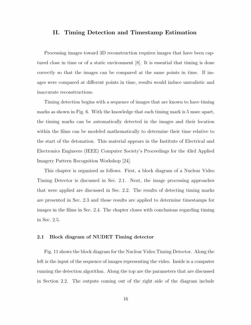
Fig. 11 shows the block diagram for the Nuclear Video Timing Detector. Along the

left is the input of the sequence of images representing the video. Inside is a computer

running the detection algorithm. Along the top are the parameters that are discussed

in Section 2.2. The outputs coming out of the right side of the diagram include

16

Figure 11. NUDET Timing detector Block Diagram.

whether a detection has occurred on a particular frame, the y-coordinate location

of where that detection is in the frame, and the interval from the last successful

detection.

2.2 Description of approaches

To accomplish the timing detection, two major approaches are used which are

called Column Sum and Circle Detection. Some algorithms also used a Change De-

tection approach to maximize the detection rate. Some features were also added

including sensing the timing column and skipping images based on predicted inter-

vals. Each of these approaches and subapproaches will be described in detail.

Column Sum.

The column sum approach takes advantage of the fact that the timing marks are

expected to be repeated in the same vertical column. The existence of a timing mark

in the column should raise the overall pixel values of that column. The difference in

17

the amount of additional pixel value could be used as the discriminator to distinguish

frames that have timing marks from frames that do not. Timing marks are about

40-60 pixels wide and need to be reduced to one number that is used to determine if

it is in the acceptable range (a timing mark without a frame), or out of the acceptable

range (a timing mark in a frame). Equation 3 shows how to arrive at the overall pixel

indicator value (V ) from an M row, for a column that is assumed to be 40 pixels wide

that has a pixel value at row m, column n of S(m,n).

V =1

40×

40∑n=1

M∑m=1

S(m,n) (3)

With an pictorial example of a timing mark and column in Fig. 9, the results of

Eq. (3) are the sum total of all the pixel values in the timing column divided by the

width of the column. One shortfall of this approach is that the timing lane needs

to be determined ahead of time. Initially this was done with human intervention,

however column sensing discusses an automated approach to this. Now that we have

a value to measure the overall light in a column, an approach must be defined for a

threshold to determine if that value is a detection of a timing mark or not.

Relative vs Global Thresholds.

Initially it was believed that an average of all the pixel sums could be used as a

baseline for a non-detection, and a certain distance (i.e. 2 standard deviations) away

from it might indicate a detection. This global threshold worked well for the first few

detections, but once the explosion occurred, the explosion influenced the pixel values

in the timing lane. Additionally, the light from the explosion would go up and down

throughout the explosion further complicating detection. A local average needed to

be established that could improve detection rates.

A relative threshold would be a moving average that “forgets” information that

18

is too far away from it. It might be an average and standard deviation of the last 25

frames. This would allow the overall baseline to adjust more quickly while still being

representative of the overall average pixel sum.

Circle Detection.

The second major approach for detecting the timing marks is to leverage the fact

that their expected shape is a circle. A Hough transform [4] might be able to detect

the circles. Sometimes the circles are faint and the image contrast can be adjusted

so that the boundaries of the circle are more pronounced. Furthermore, once the

region of the timing column is detected, the region that circles are searched for can

be reduced from the entire image to just the timing column.

Through preliminary testing, it was discovered that the width of the timing column

has an impact on the sensitivity of the circle detection. It might be thought that

restricting the image to the smallest column possible would be most beneficial as to

avoid false detections out of the column. However, the timing column needs to be

wide enough to contain enough of the edges of the circle for the Hough transform [4]

to detect. Through testing it was determined that the sweet spot for the 40 pixel

diameter timing marks was between 40 and 60 pixels.

Column Sensing.

The column sensing feature uses a Hough transform [4] to detect the circle of

expected size and restricts the search region based on that detection rather than

requiring human intervention. This feature is sensitive to false detections. If the first

circle of correct size is not a timing mark, then the region is restricted incorrectly

resulting in the processing missing detections in the entire video.

19

Change Image.

Another approach that can be combined with either Circle Detection or Column

Sum is to use a change image. By subtracting two images pixel by pixel, the changes

are more pronounced with the hope being that they are easier to detect.

Change from previous image.

Deriving a change image using the previous image is one change image approach.

At the slowest executed frame rates for the high-speed films the timing marks are

never less than 5 frames away, so a change image will still preserve the timing mark.

The change image will also reduce the effect that gradual ambient light has on the

overall bias of pixel sum. Lastly, a change from the previous image can help reduce

occlusions if they are slow moving occlusions (e.g. clouds of smoke). The downside is

that they can magnify undesired changes like scratches or imperfections in the film.

Change from shift image.

A change image can also be derived from the same image if the image is shifted

by a certain number of pixels. A change image derived from the same image would

subtract out most of the ambient light. To retain the presence of the timing mark the

image can be shifted the length of the diameter of the timing mark so that the timing

mark is shifted such that it no longer overlaps itself. This would result in a change

image that highlights the timing mark to the maximum extent possible, while still

removing a fair amount of the ambient light. This would occur at about 40 pixels,

which is the anticipated diameter of the timing marks.

This change approach is not as beneficial as changing from the previous image in

the situation of occlusions. Shifting the image also shifts the occlusions resulting in the

occlusions still existing in the change image. This is potentially helpful when an image

20

is washed out because of overexposure. In the overexposure case, the overexposure is

subtracted out, making the timing mark more pronounced because the overexposure

noise is reduced.

Interval sensing and interval skipping.

Once an approach can effectively detect most of the timing marks, it is possible

to speed up the processing by skipping over images that are likely not to have timing

marks because they are too close to the previous timing mark. One simple example

might be taking advantage of the fact that there are at least 5 frames between timing

marks. If a mark is detected, then the processing can jump forward at least 5 frames

before resuming. This would speed up the processing considerably because the image

processing is the largest consumer of processing resources in the algorithm. It also

reduces the potential for a false detection because images that are known to not have

marks are not checked.

This basic case can be adapted to increase the timing interval over time to fit

the film interval better. The timings marks gradually spread out in frames as time

passes. That’s because the timing interval is consistent, but the film spins faster as

the weight on the spool of film decreases. While the nominal speed of the film is 2500

frames per second, this acceleration effect can result in a film speed over 3000 frames

per second.

Consider an approach that calculates the previous timing interval based on the two

most recent timing detections and applies this interval to the future. This allows the

timing interval to adapt but it is also sensitive to the effect of missed detections and

false detections. There are some cases where the interval decreases by one because

of where the detections fall within the frames. For example, when detections are

occurring from the middle of one frame to the middle of another the interval might

21

be eight. But if the detection occurs late in the first frame and early in the later

frame, that same interval would be seven frames apart.

A missed detection would be catastrophic for the procedure. If a detection were

missed that would mean that the interval would double. The result of a doubled

interval would skip over every other timing mark. Successive missed timing marks

would increase the timing interval further compounding the problem. Thus, being

conservative, the interval is reduced by one to ensure detections are not missed.

Fortunately, the spreading out of timing marks is gradual. Intervals should never

double immediately and if they do, it can be assumed that a detection was missed

and the interval reduced appropriately.

Combining approaches.

It is intuitive that combining some approaches would be beneficial when the ap-

proaches dovetail, while other approaches do not combine well. For example, interval

skipping would not work well with an approach that only detects 50% of timing marks.

However, interval skipping works well at reducing false positives when combined with

a detection scheme that finds 90% of timing marks. It is also apparent, that if change

images are used, that they are mutually exclusive so only one of the change image

approaches can be used, not both of them. Rather than subtracting out unwanted

light and exposure, a double change image would add more differencing back into the

final result.

The two major approaches (column sum and circle detect) were tried as AND

combinations and OR in attempt to create one superior model. While the AND case

had fewer false positive detections, it was at the expense of missing good detections

(i.e true positives). The OR case was similar, except while it maximized true positive

detections, it also increased false positive detections.

22

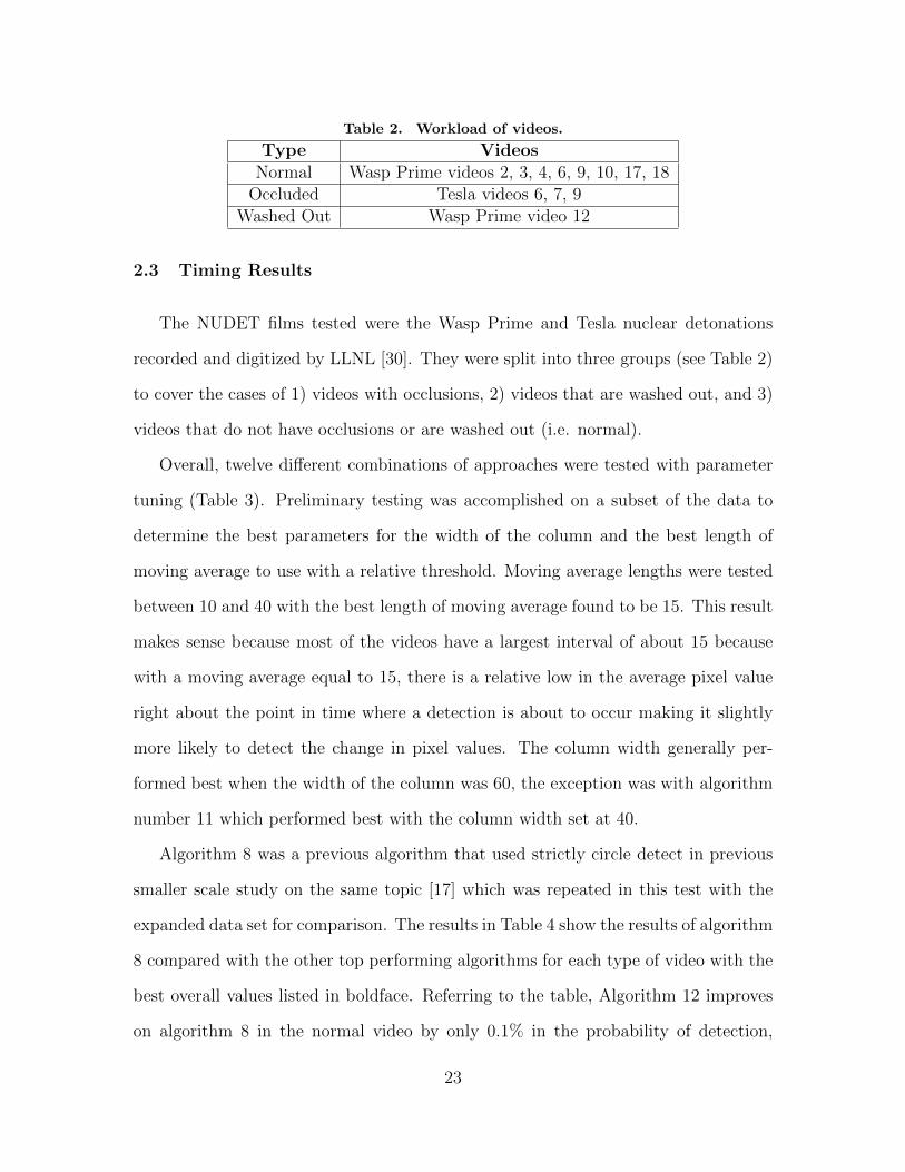
Table 2. Workload of videos.

Type VideosNormal Wasp Prime videos 2, 3, 4, 6, 9, 10, 17, 18

Occluded Tesla videos 6, 7, 9Washed Out Wasp Prime video 12

2.3 Timing Results

The NUDET films tested were the Wasp Prime and Tesla nuclear detonations

recorded and digitized by LLNL [30]. They were split into three groups (see Table 2)

to cover the cases of 1) videos with occlusions, 2) videos that are washed out, and 3)

videos that do not have occlusions or are washed out (i.e. normal).

Overall, twelve different combinations of approaches were tested with parameter

tuning (Table 3). Preliminary testing was accomplished on a subset of the data to

determine the best parameters for the width of the column and the best length of

moving average to use with a relative threshold. Moving average lengths were tested

between 10 and 40 with the best length of moving average found to be 15. This result

makes sense because most of the videos have a largest interval of about 15 because

with a moving average equal to 15, there is a relative low in the average pixel value

right about the point in time where a detection is about to occur making it slightly

more likely to detect the change in pixel values. The column width generally per-

formed best when the width of the column was 60, the exception was with algorithm

number 11 which performed best with the column width set at 40.

Algorithm 8 was a previous algorithm that used strictly circle detect in previous

smaller scale study on the same topic [17] which was repeated in this test with the

expanded data set for comparison. The results in Table 4 show the results of algorithm

8 compared with the other top performing algorithms for each type of video with the

best overall values listed in boldface. Referring to the table, Algorithm 12 improves

on algorithm 8 in the normal video by only 0.1% in the probability of detection,

23

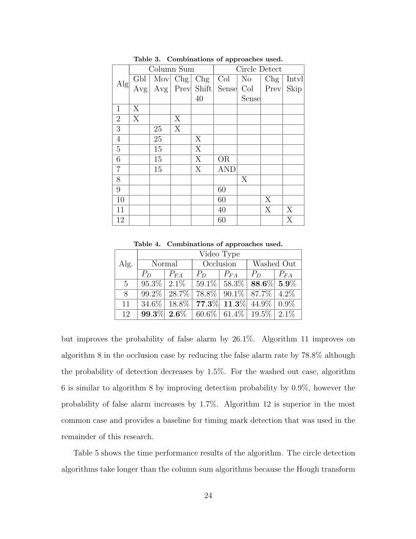
Table 3. Combinations of approaches used.

Alg

Column Sum Circle DetectGblAvg

MovAvg

ChgPrev

ChgShift40

ColSense

NoColSense

ChgPrev

IntvlSkip

1 X2 X X3 25 X4 25 X5 15 X6 15 X OR7 15 X AND8 X9 6010 60 X11 40 X X12 60 X

Table 4. Combinations of approaches used.

Alg.Video Type

Normal Occlusion Washed OutPD PFA PD PFA PD PFA

5 95.3% 2.1% 59.1% 58.3% 88.6% 5.9%8 99.2% 28.7% 78.8% 90.1% 87.7% 4.2%11 34.6% 18.8% 77.3% 11.3% 44.9% 0.9%12 99.3% 2.6% 60.6% 61.4% 19.5% 2.1%

but improves the probability of false alarm by 26.1%. Algorithm 11 improves on

algorithm 8 in the occlusion case by reducing the false alarm rate by 78.8% although

the probability of detection decreases by 1.5%. For the washed out case, algorithm

6 is similar to algorithm 8 by improving detection probability by 0.9%, however the

probability of false alarm increases by 1.7%. Algorithm 12 is superior in the most

common case and provides a baseline for timing mark detection that was used in the

remainder of this research.

Table 5 shows the time performance results of the algorithm. The circle detection

algorithms take longer than the column sum algorithms because the Hough transform

24

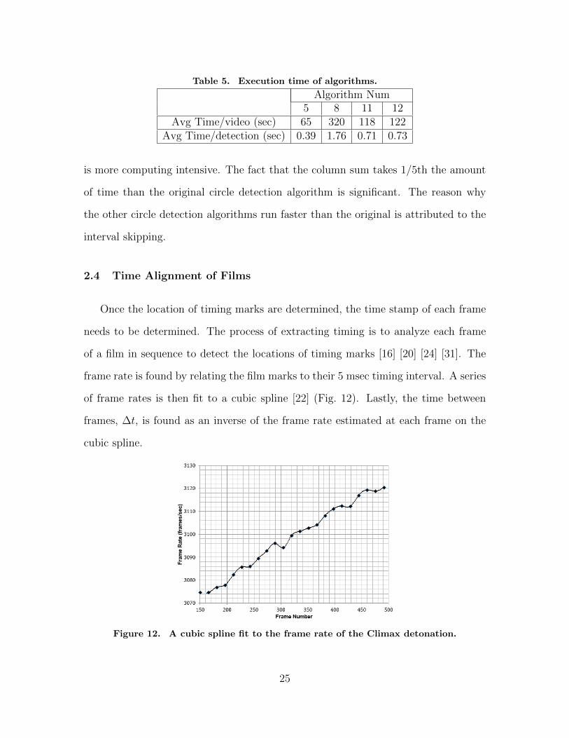
Table 5. Execution time of algorithms.

Algorithm Num5 8 11 12

Avg Time/video (sec) 65 320 118 122Avg Time/detection (sec) 0.39 1.76 0.71 0.73

is more computing intensive. The fact that the column sum takes 1/5th the amount

of time than the original circle detection algorithm is significant. The reason why

the other circle detection algorithms run faster than the original is attributed to the

interval skipping.

2.4 Time Alignment of Films

Once the location of timing marks are determined, the time stamp of each frame

needs to be determined. The process of extracting timing is to analyze each frame

of a film in sequence to detect the locations of timing marks [16] [20] [24] [31]. The

frame rate is found by relating the film marks to their 5 msec timing interval. A series

of frame rates is then fit to a cubic spline [22] (Fig. 12). Lastly, the time between

frames, ∆t, is found as an inverse of the frame rate estimated at each frame on the

cubic spline.

Figure 12. A cubic spline fit to the frame rate of the Climax detonation.

25

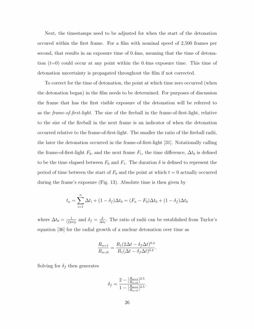
Next, the timestamps need to be adjusted for when the start of the detonation

occured within the first frame. For a film with nominal speed of 2,500 frames per

second, that results in an exposure time of 0.4ms, meaning that the time of detona-

tion (t=0) could occur at any point within the 0.4ms exposure time. This time of

detonation uncertainty is propagated throughout the film if not corrected.

To correct for the time of detonation, the point at which time zero occurred (when

the detonation began) in the film needs to be determined. For purposes of discussion

the frame that has the first visible exposure of the detonation will be referred to

as the frame-of-first-light. The size of the fireball in the frame-of-first-light, relative

to the size of the fireball in the next frame is an indicator of when the detonation

occurred relative to the frame-of-first-light. The smaller the ratio of the fireball radii,

the later the detonation occurred in the frame-of-first-light [31]. Notationally calling

the frame-of-first-light F0, and the next frame F1, the time difference, ∆t0 is defined

to be the time elapsed between F0 and F1. The duration δ is defined to represent the

period of time between the start of F0 and the point at which t = 0 actually occurred

during the frame’s exposure (Fig. 13). Absolute time is then given by

tn =n∑i=1

∆ti + (1− δf )∆t0 = (Fn − F0)∆t0 + (1− δf )∆t0

where ∆t0 = 1(fps)0

and δf = δ∆t0

. The ratio of radii can be established from Taylor’s

equation [36] for the radial growth of a nuclear detonation over time as

Rn=1

Rn=0

=R1(2∆t− δf∆t)0.4

R1(∆t− δf∆t)0.4.

Solving for δf then generates

δf =2− [Rn=1

Rn=0]2.5

1− [Rn=1

Rn=0]2.5

.

26

Finally, the time δ = δf∆t. To validate that the timing was correct, the radius of a

Figure 13. The methodology to align the timing of films with time t = 0 [31].

detonation from collection sites with multiple cameras were compared to each other

with their radii plotted over time. With nearly identical focal lengths, the expectation

was that frames of the same time would have the same radius in the nuclear detonation

regardless of whether they were captured by fast or slow camera rates. This fact was

verified in each film where there were multiple cameras from the same collection site.

Fig. 14 shows an example output of the time analyzed from a collection site of the

Tesla detonation that had six cameras. Other than the outliers caused by errors in

the radius detection, the prevailing trend of radius growth over time is confirmed.

2.5 Timing Conclusions

This experiment explored several approaches to detecting timing marks in nuclear

detection video. It was determined that the previous best method of basic circle

detection can be improved upon by adding interval skipping which reduces the false

positive rate by 26.1% and reduces the processing time by a factor of 2.5. When

detection in occluded videos is required, an approach that includes both a change

detection from the previous image and interval skipping reduces the false positive

27

Figure 14. A plot of radius growth over time based on time estimates from multiplecameras from Tesla Truck 7. A few outliers exist that were a result of errors in theautomated detection of the radius of the detonation.

rate by 78.8% and cuts processing time by a factor of 2.5. When detection in washed

out or overexposed videos is required, the processing time can be cut significantly

with similar detection results.

With timing marks detected accurately, the timestamp of each frame can be es-

timated by fitting the frame rates to a cubic spline. Timestamps are adjusted based

on applying Taylor’s equation [36] to the radius of the fireball in the frame-of-first-

light. The end result is that each frame is timestamped relative to the start of the

detonation.

28

III. Subsphere Detection

With the videos temporally aligned, the focus shifts to detecting features on the

NUDETS that can be used to estimate volume or be matched across wide viewpoints.

The first feature to be detected are subspheres (Fig. 8). These features are visible

areas of deformity in the detonation likely caused by obstructions that degrade the

spherical uniformity of the detonation shock wave. This chapter summarizes an ex-

periment set up to determine whether dimensionality reduction with classification is

effective in detecting subspheres in the NUDETs. Furthermore, it helps determine

what combinations of parameters and dimensions help produce the best results to

detect subspheres in the films.

The chapter is organized beginning with a block diagram in Sec. 3.1. The results of

applying the nuclear subsphere detection approaches are discussed in Sec. 3.2. Lastly,

conclusions are drawn in Sec. 3.3.

3.1 Block diagram

Fig. 15 shows a block diagram for the system that is designed to detect subspheres

in a NUDET image aptly named the NUDET Subsphere Detector (NSD). Each of the

parameters discussed in this algorithm synopsis is described in detail. The NSD is

broken into two primary parts: the learner, and the detector. The learner’s function

is to use the truth information and dimensionality reduction algorithms to determine

which dimensions are best for the detector to use. The learner imports an image and

applies a filter to the image. Iterating through each pixel in the image, the dimension

extractor extracts 300 dimensions from the surrounding pixels based on the kernel size.

It then applies a dimensionality reduction algorithm to the dimensions to determine

the most relevant dimensions. Using the most relevant dimensions, a Mahalanobis-

29

Figure 15. Block Diagram for Subsphere Detector.

based classifier determines if the pixel in question is a subsphere edge or not. Lastly,

the detected pixels are clustered into neighboring detected pixels to create the list

of subspheres with their corresponding locations. When the learner is complete, the

best dimensions are then used as the basis of the detector to detect the subspheres.

The detector then runs similar to the learner without the dimensionality reduction.

It uses the dimensionality reduction’s recommended dimensions to determine which

pixels have subspheres in them.

Inputs.

Along the left side of the block diagram (Fig. 15) are the inputs, which are the

subject image and a human interpretation of where subspheres exist in the image (i.e

truth data). The truth data is used initially in the dimensionality reduction to “learn”

30

which dimensions are the best dimensions to use in detection. Later, in validation

and testing, it is used to determine whether a detection is a true positive or false

positive.

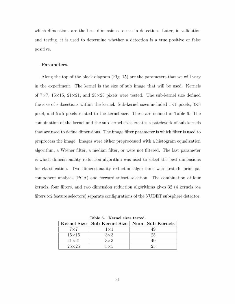
Parameters.

Along the top of the block diagram (Fig. 15) are the parameters that we will vary

in the experiment. The kernel is the size of sub image that will be used. Kernels

of 7×7, 15×15, 21×21, and 25×25 pixels were tested. The sub-kernel size defined

the size of subsections within the kernel. Sub-kernel sizes included 1×1 pixels, 3×3

pixel, and 5×5 pixels related to the kernel size. These are defined in Table 6. The

combination of the kernel and the sub-kernel sizes creates a patchwork of sub-kernels

that are used to define dimensions. The image filter parameter is which filter is used to

preprocess the image. Images were either preprocessed with a histogram equalization

algorithm, a Wiener filter, a median filter, or were not filtered. The last parameter

is which dimensionality reduction algorithm was used to select the best dimensions

for classification. Two dimensionality reduction algorithms were tested: principal

component analysis (PCA) and forward subset selection. The combination of four

kernels, four filters, and two dimension reduction algorithms gives 32 (4 kernels ×4

filters×2 feature selectors) separate configurations of the NUDET subsphere detector.

Table 6. Kernel sizes tested.

Kernel Size Sub Kernel Size Num. Sub Kernels7×7 1×1 49

15×15 3×3 2521×21 3×3 4925×25 5×5 25

31

Outputs.

The outputs of the NSD include whether a subsphere edge detection occurred,

and at what X and Y pixel.

3.2 Subsphere Detection Results

To analyze which algorithm/kernel/filter combination performed best, the data

was analyzed using a Receiver Operating Characteristic (ROC) curve. A ROC curve

plots the results of the Hit Rate (Eq. 4) along the y-axis and False Alarm Rate

(Eq. 5) along the x-axis. Each algorithm/kernel/filter combination was plotted on

a ROC curve for the top 50 dimensions according to either the PCA or sequential

forward subset (SFS) algorithm. ROC curves provide a way to graphically determine

what the maximum Hit Rate while minimizing the False Alarm Rate.

Hit Rate =True Positive

True Positive+ False Negative(4)

False Alarm Rate =False Positive

False Positive+ True Negative(5)

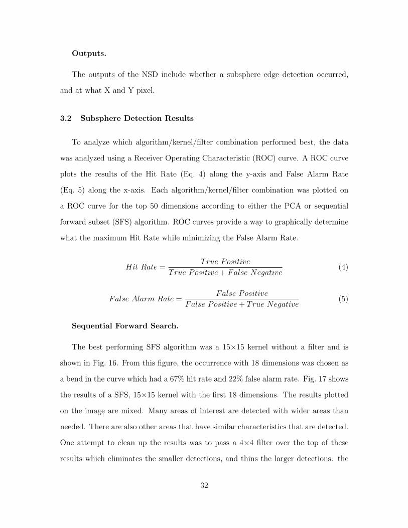
Sequential Forward Search.

The best performing SFS algorithm was a 15×15 kernel without a filter and is

shown in Fig. 16. From this figure, the occurrence with 18 dimensions was chosen as

a bend in the curve which had a 67% hit rate and 22% false alarm rate. Fig. 17 shows

the results of a SFS, 15×15 kernel with the first 18 dimensions. The results plotted

on the image are mixed. Many areas of interest are detected with wider areas than

needed. There are also other areas that have similar characteristics that are detected.

One attempt to clean up the results was to pass a 4×4 filter over the top of these

results which eliminates the smaller detections, and thins the larger detections. the

32

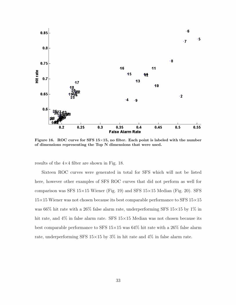
Figure 16. ROC curve for SFS 15×15, no filter. Each point is labeled with the numberof dimensions representing the Top N dimensions that were used.

results of the 4×4 filter are shown in Fig. 18.

Sixteen ROC curves were generated in total for SFS which will not be listed

here, however other examples of SFS ROC curves that did not perform as well for

comparison was SFS 15×15 Wiener (Fig. 19) and SFS 15×15 Median (Fig. 20). SFS

15×15 Wiener was not chosen because its best comparable performance to SFS 15×15

was 66% hit rate with a 26% false alarm rate, underperforming SFS 15×15 by 1% in

hit rate, and 4% in false alarm rate. SFS 15×15 Median was not chosen because its

best comparable performance to SFS 15×15 was 64% hit rate with a 26% false alarm

rate, underperforming SFS 15×15 by 3% in hit rate and 4% in false alarm rate.

33

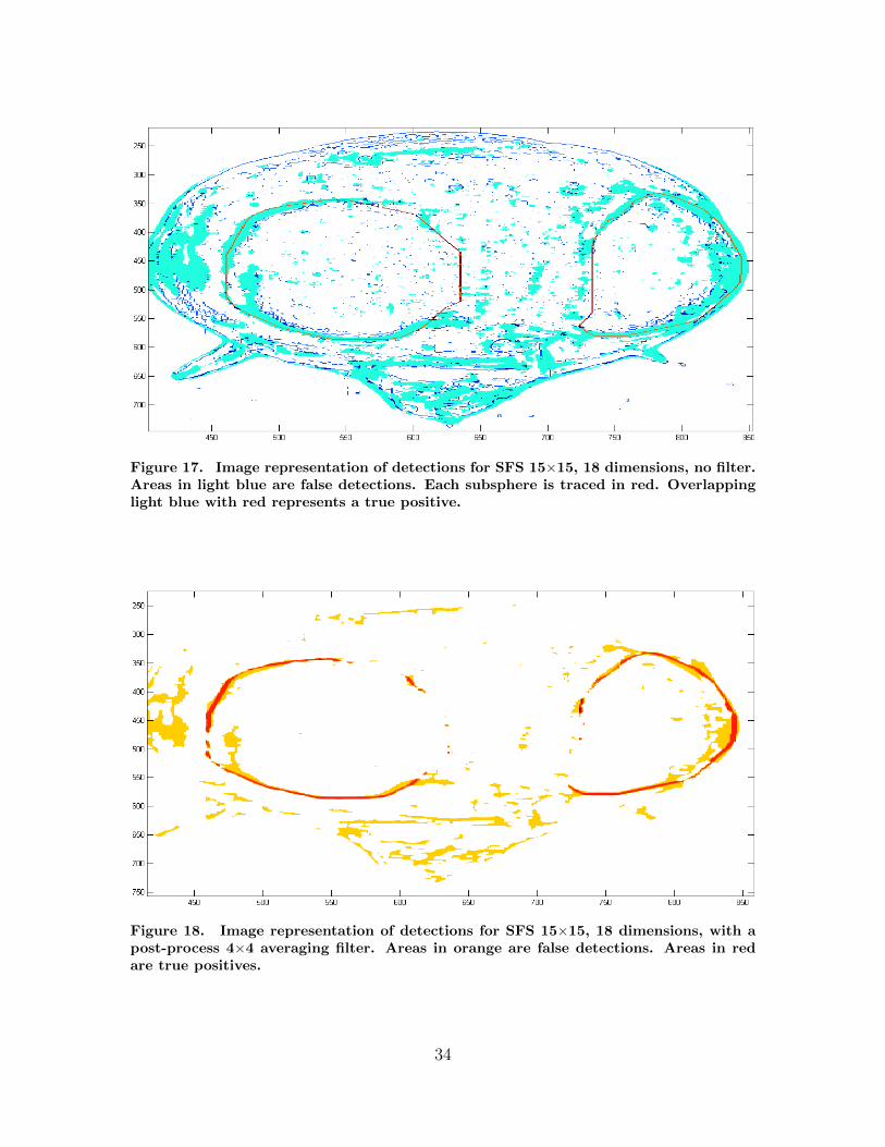
Figure 17. Image representation of detections for SFS 15×15, 18 dimensions, no filter.Areas in light blue are false detections. Each subsphere is traced in red. Overlappinglight blue with red represents a true positive.

Figure 18. Image representation of detections for SFS 15×15, 18 dimensions, with apost-process 4×4 averaging filter. Areas in orange are false detections. Areas in redare true positives.

34

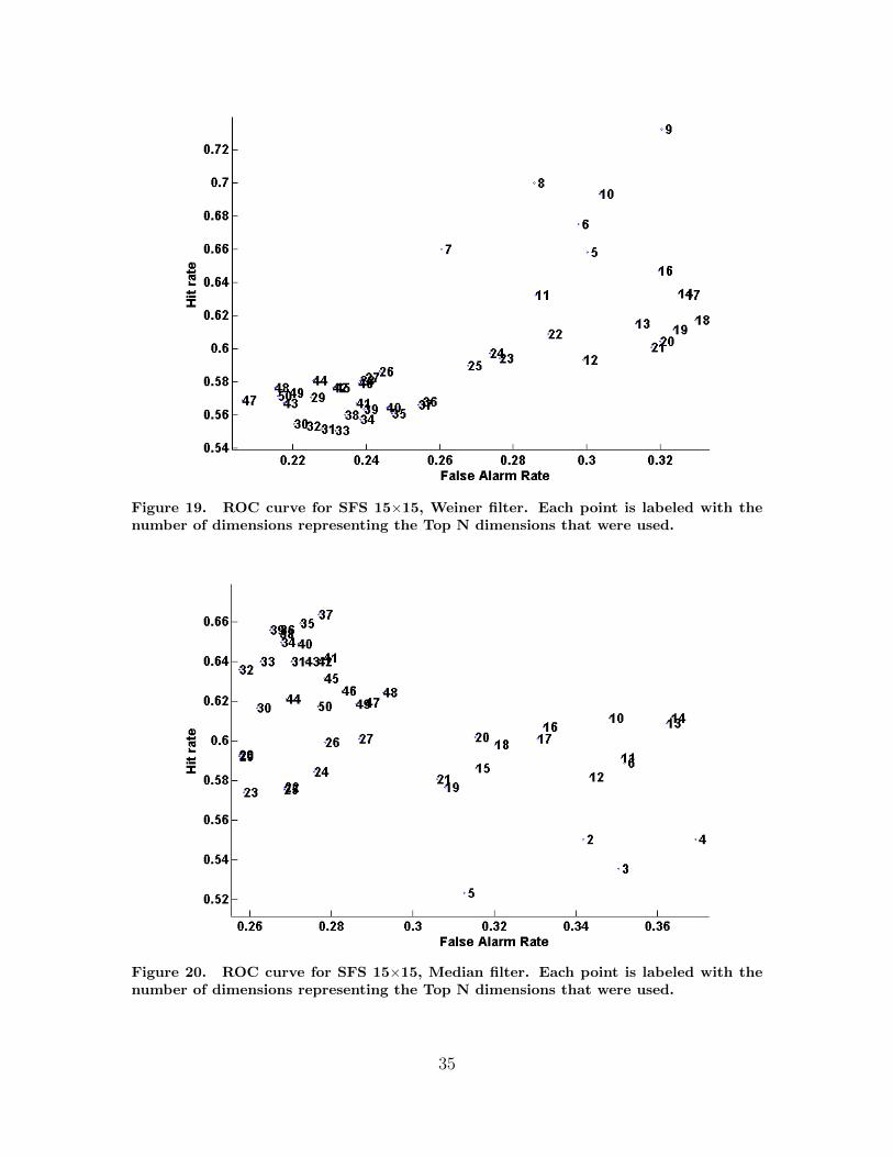
Figure 19. ROC curve for SFS 15×15, Weiner filter. Each point is labeled with thenumber of dimensions representing the Top N dimensions that were used.

Figure 20. ROC curve for SFS 15×15, Median filter. Each point is labeled with thenumber of dimensions representing the Top N dimensions that were used.

35

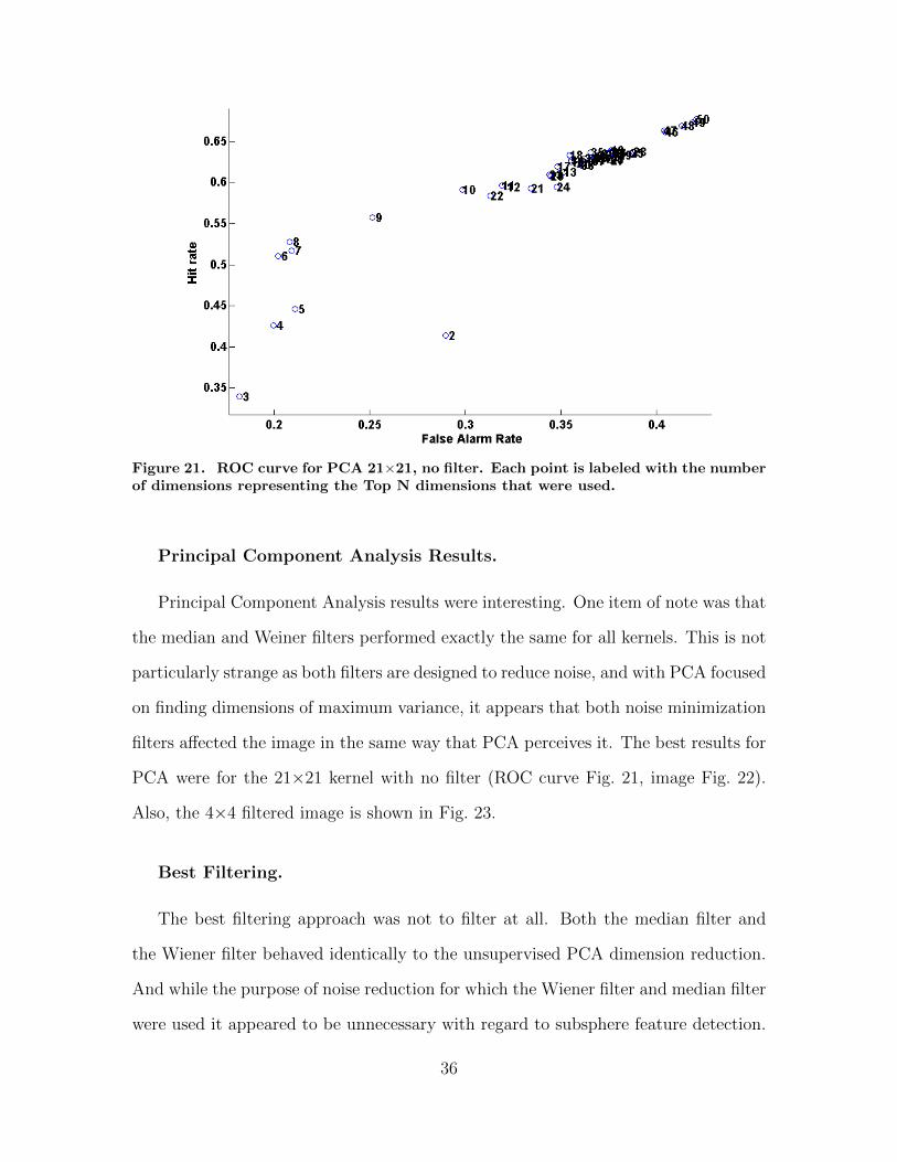
Figure 21. ROC curve for PCA 21×21, no filter. Each point is labeled with the numberof dimensions representing the Top N dimensions that were used.

Principal Component Analysis Results.

Principal Component Analysis results were interesting. One item of note was that

the median and Weiner filters performed exactly the same for all kernels. This is not

particularly strange as both filters are designed to reduce noise, and with PCA focused

on finding dimensions of maximum variance, it appears that both noise minimization

filters affected the image in the same way that PCA perceives it. The best results for

PCA were for the 21×21 kernel with no filter (ROC curve Fig. 21, image Fig. 22).

Also, the 4×4 filtered image is shown in Fig. 23.

Best Filtering.

The best filtering approach was not to filter at all. Both the median filter and

the Wiener filter behaved identically to the unsupervised PCA dimension reduction.

And while the purpose of noise reduction for which the Wiener filter and median filter

were used it appeared to be unnecessary with regard to subsphere feature detection.

36

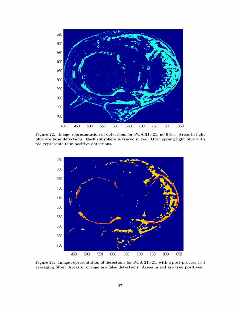
Figure 22. Image representation of detections for PCA 21×21, no filter. Areas in lightblue are false detections. Each subsphere is traced in red. Overlapping light blue withred represents true positive detections.

Figure 23. Image representation of detections for PCA 21×21, with a post-process 4×4averaging filter. Areas in orange are false detections. Areas in red are true positives.

37

There are other images and videos in the NUDET data set that these filters may

apply better to, but it appears that their application to images that are clear and

relatively unaffected by noise are not beneficial in subsphere feature detection.

3.3 Conclusions

This chapter tested which combination of kernels (7×7, 15×15, 21×21, and 25×25

pixels), dimension reduction algorithms (SFS, PCA), and filters (no filter, histogram

equalization, Wiener, and median) worked best to detect the edges of a subsphere in

a nuclear detonation image. The best result had a 67% hit rate and 22% false alarm

rate and was SFS 15×15 with no filter, with the top 18 dimensions. These results

were further improved by applying a 4×4 averaging filter and is shown in Fig. 18.

The location of subsphere features are used in estimating the volume of NUDETs

which is discussed in Chapter VII.

38

IV. Hotspot Detection

The next feature to be detected are hotspots (Fig. 9). These are spots on the

surface of the detonation that are at higher temperature relative to the local area

around it that cause it to be brighter. This chapter discusses a process that is defined

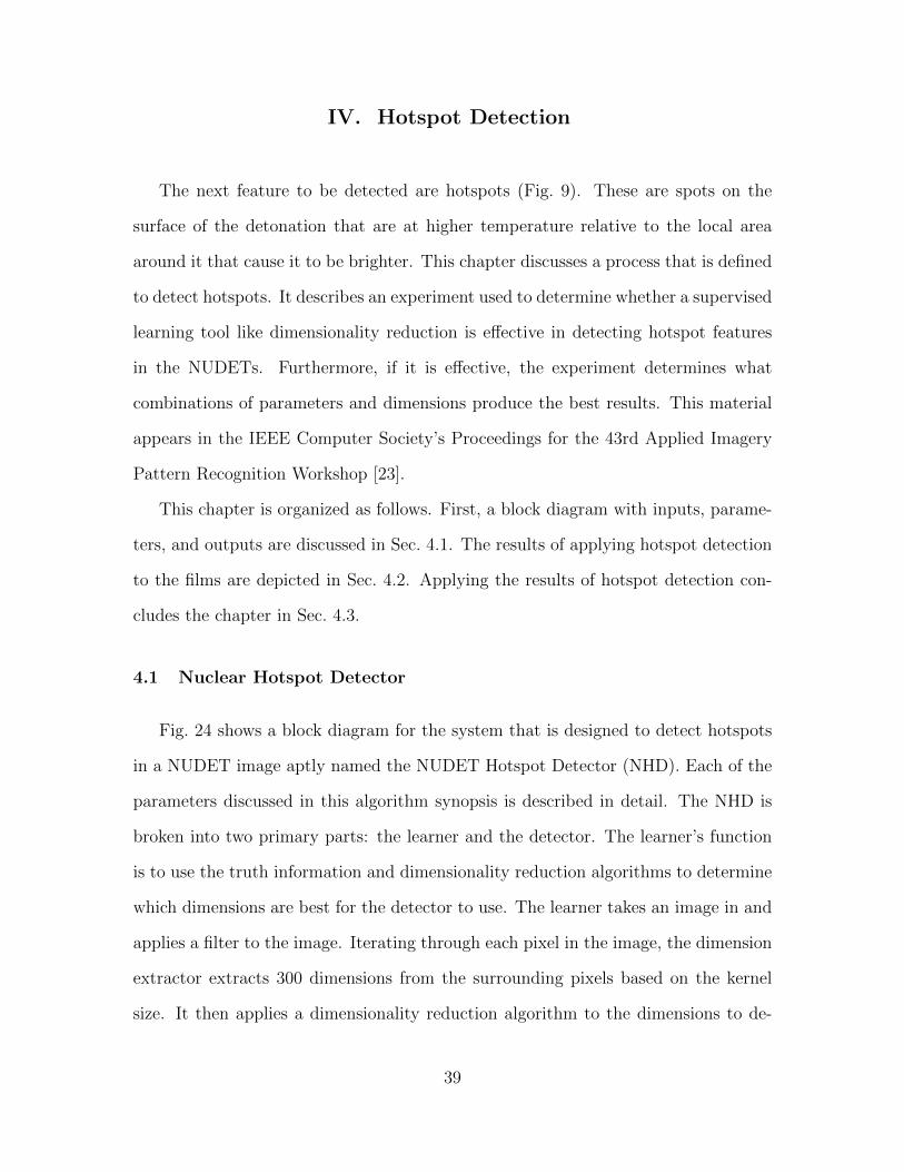
to detect hotspots. It describes an experiment used to determine whether a supervised

learning tool like dimensionality reduction is effective in detecting hotspot features

in the NUDETs. Furthermore, if it is effective, the experiment determines what

combinations of parameters and dimensions produce the best results. This material

appears in the IEEE Computer Society’s Proceedings for the 43rd Applied Imagery

Pattern Recognition Workshop [23].

This chapter is organized as follows. First, a block diagram with inputs, parame-

ters, and outputs are discussed in Sec. 4.1. The results of applying hotspot detection

to the films are depicted in Sec. 4.2. Applying the results of hotspot detection con-

cludes the chapter in Sec. 4.3.

4.1 Nuclear Hotspot Detector

Fig. 24 shows a block diagram for the system that is designed to detect hotspots

in a NUDET image aptly named the NUDET Hotspot Detector (NHD). Each of the

parameters discussed in this algorithm synopsis is described in detail. The NHD is

broken into two primary parts: the learner and the detector. The learner’s function

is to use the truth information and dimensionality reduction algorithms to determine

which dimensions are best for the detector to use. The learner takes an image in and

applies a filter to the image. Iterating through each pixel in the image, the dimension

extractor extracts 300 dimensions from the surrounding pixels based on the kernel

size. It then applies a dimensionality reduction algorithm to the dimensions to de-

39

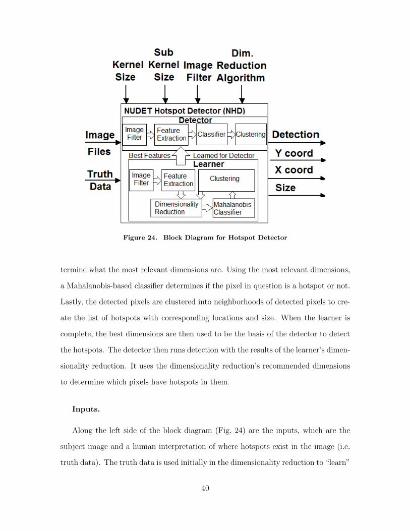
Figure 24. Block Diagram for Hotspot Detector

termine what the most relevant dimensions are. Using the most relevant dimensions,

a Mahalanobis-based classifier determines if the pixel in question is a hotspot or not.

Lastly, the detected pixels are clustered into neighborhoods of detected pixels to cre-

ate the list of hotspots with corresponding locations and size. When the learner is

complete, the best dimensions are then used to be the basis of the detector to detect

the hotspots. The detector then runs detection with the results of the learner’s dimen-

sionality reduction. It uses the dimensionality reduction’s recommended dimensions

to determine which pixels have hotspots in them.

Inputs.

Along the left side of the block diagram (Fig. 24) are the inputs, which are the

subject image and a human interpretation of where hotspots exist in the image (i.e.

truth data). The truth data is used initially in the dimensionality reduction to “learn”

40

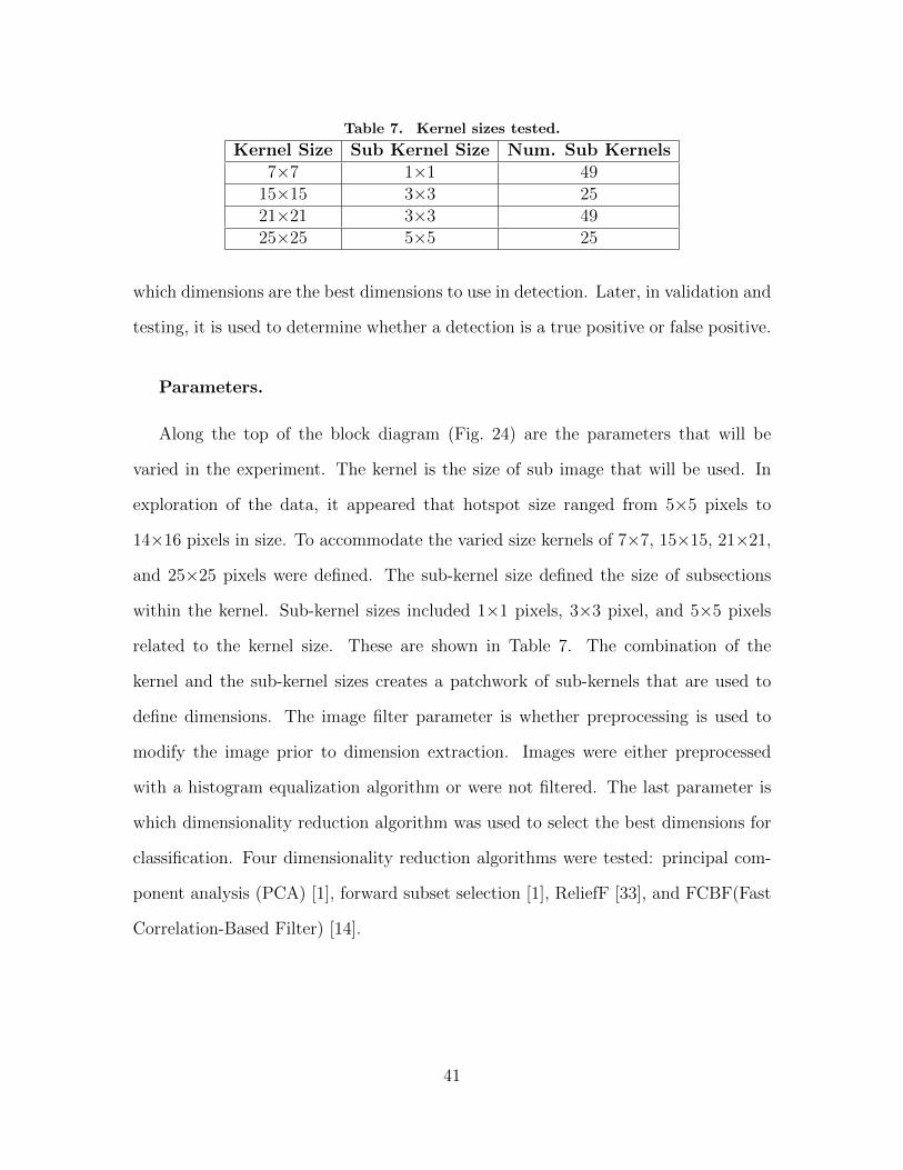
Table 7. Kernel sizes tested.

Kernel Size Sub Kernel Size Num. Sub Kernels7×7 1×1 49

15×15 3×3 2521×21 3×3 4925×25 5×5 25

which dimensions are the best dimensions to use in detection. Later, in validation and

testing, it is used to determine whether a detection is a true positive or false positive.

Parameters.

Along the top of the block diagram (Fig. 24) are the parameters that will be

varied in the experiment. The kernel is the size of sub image that will be used. In

exploration of the data, it appeared that hotspot size ranged from 5×5 pixels to

14×16 pixels in size. To accommodate the varied size kernels of 7×7, 15×15, 21×21,

and 25×25 pixels were defined. The sub-kernel size defined the size of subsections

within the kernel. Sub-kernel sizes included 1×1 pixels, 3×3 pixel, and 5×5 pixels

related to the kernel size. These are shown in Table 7. The combination of the

kernel and the sub-kernel sizes creates a patchwork of sub-kernels that are used to

define dimensions. The image filter parameter is whether preprocessing is used to

modify the image prior to dimension extraction. Images were either preprocessed

with a histogram equalization algorithm or were not filtered. The last parameter is

which dimensionality reduction algorithm was used to select the best dimensions for

classification. Four dimensionality reduction algorithms were tested: principal com-

ponent analysis (PCA) [1], forward subset selection [1], ReliefF [33], and FCBF(Fast

Correlation-Based Filter) [14].

41

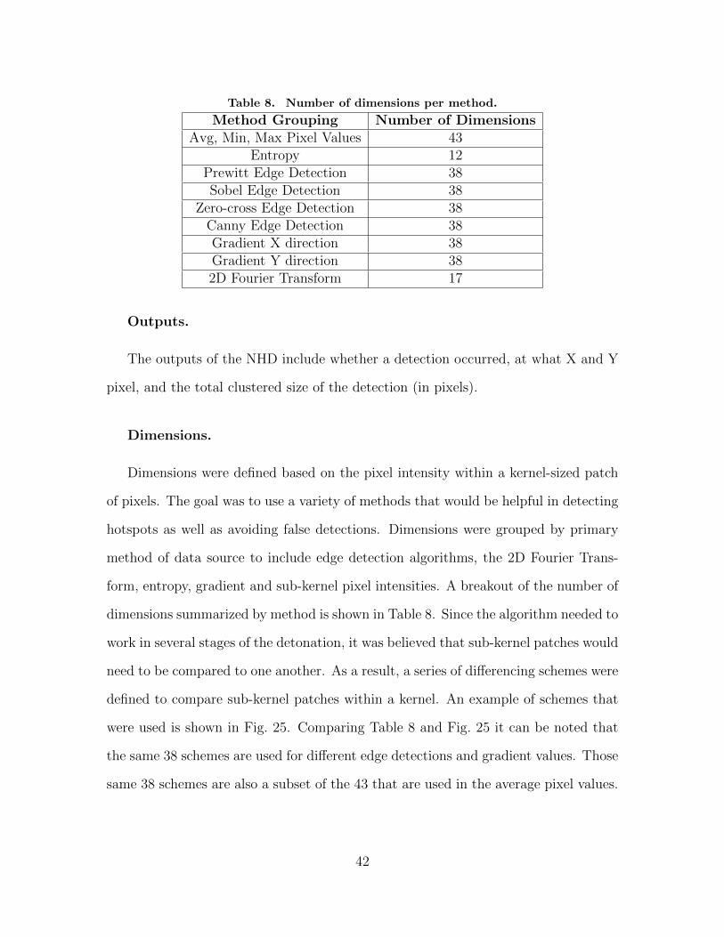
Table 8. Number of dimensions per method.

Method Grouping Number of DimensionsAvg, Min, Max Pixel Values 43

Entropy 12Prewitt Edge Detection 38Sobel Edge Detection 38

Zero-cross Edge Detection 38Canny Edge Detection 38Gradient X direction 38Gradient Y direction 382D Fourier Transform 17

Outputs.

The outputs of the NHD include whether a detection occurred, at what X and Y

pixel, and the total clustered size of the detection (in pixels).

Dimensions.

Dimensions were defined based on the pixel intensity within a kernel-sized patch

of pixels. The goal was to use a variety of methods that would be helpful in detecting

hotspots as well as avoiding false detections. Dimensions were grouped by primary

method of data source to include edge detection algorithms, the 2D Fourier Trans-

form, entropy, gradient and sub-kernel pixel intensities. A breakout of the number of

dimensions summarized by method is shown in Table 8. Since the algorithm needed to

work in several stages of the detonation, it was believed that sub-kernel patches would

need to be compared to one another. As a result, a series of differencing schemes were

defined to compare sub-kernel patches within a kernel. An example of schemes that

were used is shown in Fig. 25. Comparing Table 8 and Fig. 25 it can be noted that

the same 38 schemes are used for different edge detections and gradient values. Those

same 38 schemes are also a subset of the 43 that are used in the average pixel values.

42

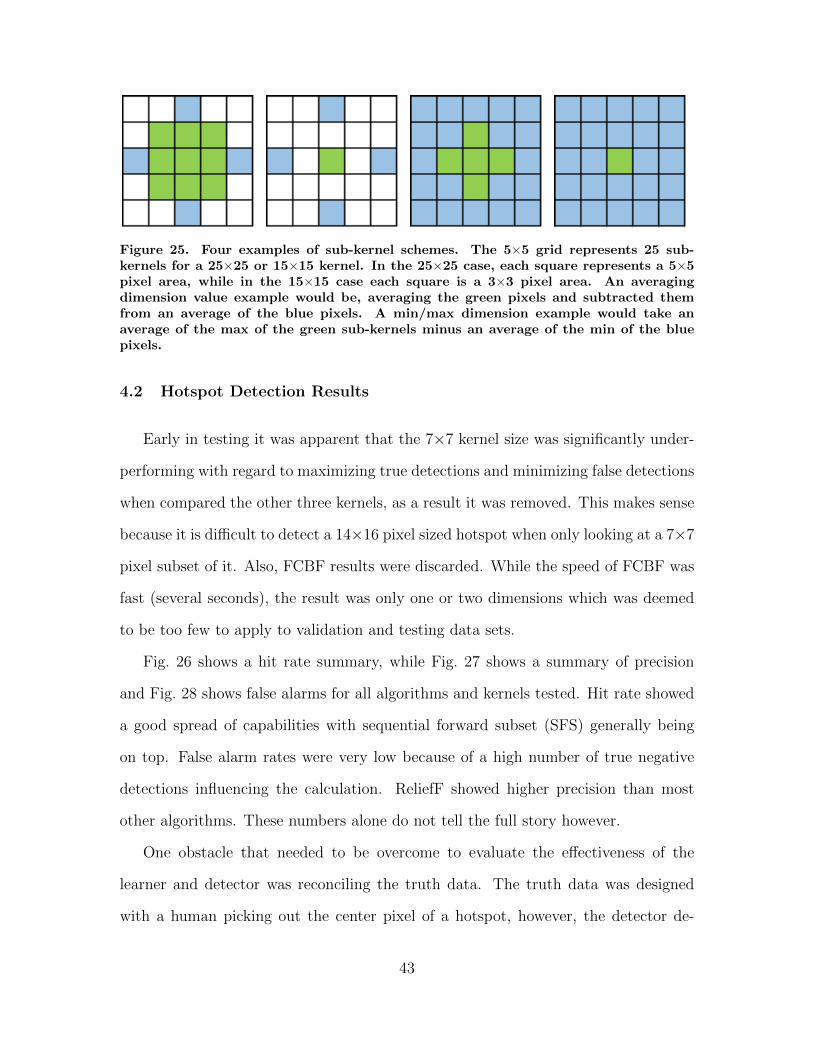
Figure 25. Four examples of sub-kernel schemes. The 5×5 grid represents 25 sub-kernels for a 25×25 or 15×15 kernel. In the 25×25 case, each square represents a 5×5pixel area, while in the 15×15 case each square is a 3×3 pixel area. An averagingdimension value example would be, averaging the green pixels and subtracted themfrom an average of the blue pixels. A min/max dimension example would take anaverage of the max of the green sub-kernels minus an average of the min of the bluepixels.

4.2 Hotspot Detection Results

Early in testing it was apparent that the 7×7 kernel size was significantly under-

performing with regard to maximizing true detections and minimizing false detections

when compared the other three kernels, as a result it was removed. This makes sense

because it is difficult to detect a 14×16 pixel sized hotspot when only looking at a 7×7

pixel subset of it. Also, FCBF results were discarded. While the speed of FCBF was

fast (several seconds), the result was only one or two dimensions which was deemed

to be too few to apply to validation and testing data sets.

Fig. 26 shows a hit rate summary, while Fig. 27 shows a summary of precision

and Fig. 28 shows false alarms for all algorithms and kernels tested. Hit rate showed

a good spread of capabilities with sequential forward subset (SFS) generally being

on top. False alarm rates were very low because of a high number of true negative

detections influencing the calculation. ReliefF showed higher precision than most

other algorithms. These numbers alone do not tell the full story however.

One obstacle that needed to be overcome to evaluate the effectiveness of the

learner and detector was reconciling the truth data. The truth data was designed

with a human picking out the center pixel of a hotspot, however, the detector de-

43

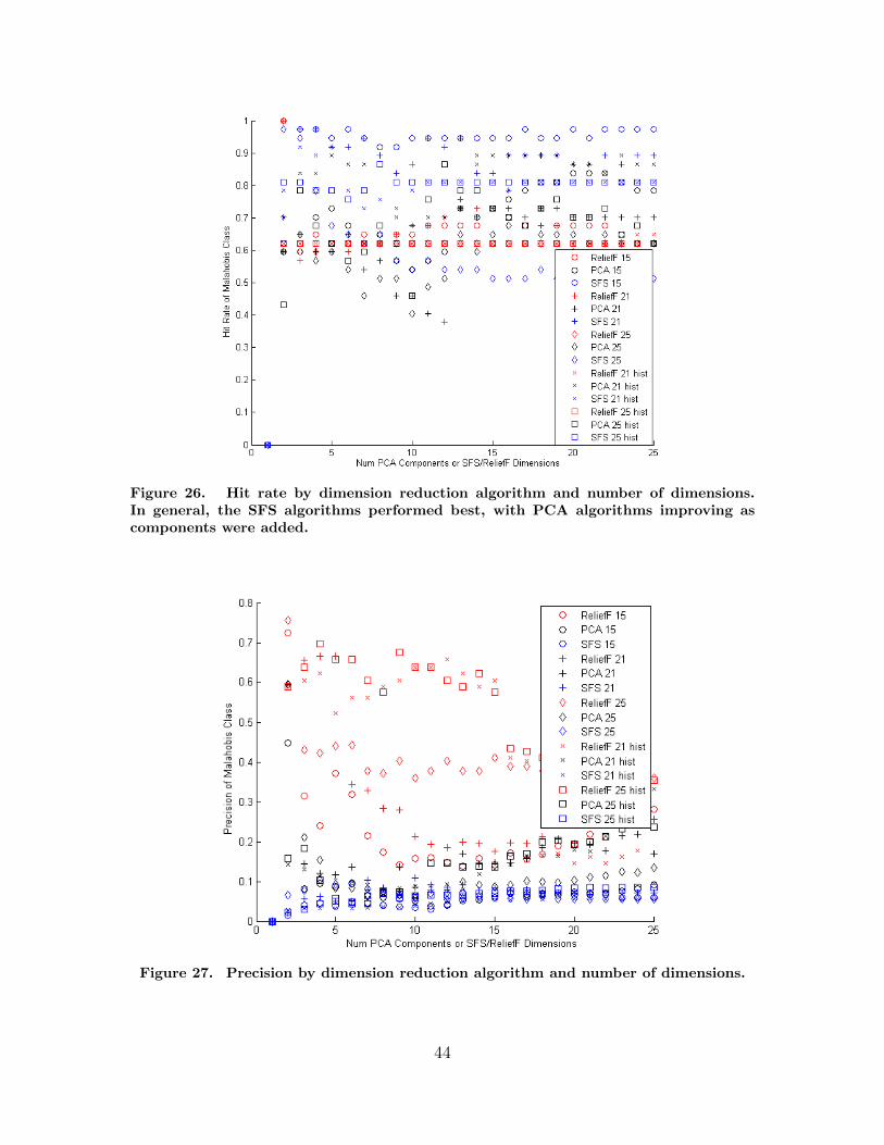
Figure 26. Hit rate by dimension reduction algorithm and number of dimensions.In general, the SFS algorithms performed best, with PCA algorithms improving ascomponents were added.

Figure 27. Precision by dimension reduction algorithm and number of dimensions.

44

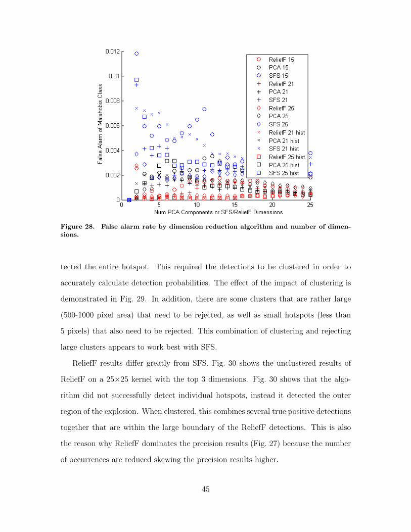
Figure 28. False alarm rate by dimension reduction algorithm and number of dimen-sions.

tected the entire hotspot. This required the detections to be clustered in order to

accurately calculate detection probabilities. The effect of the impact of clustering is

demonstrated in Fig. 29. In addition, there are some clusters that are rather large

(500-1000 pixel area) that need to be rejected, as well as small hotspots (less than

5 pixels) that also need to be rejected. This combination of clustering and rejecting

large clusters appears to work best with SFS.

ReliefF results differ greatly from SFS. Fig. 30 shows the unclustered results of

ReliefF on a 25×25 kernel with the top 3 dimensions. Fig. 30 shows that the algo-

rithm did not successfully detect individual hotspots, instead it detected the outer

region of the explosion. When clustered, this combines several true positive detections

together that are within the large boundary of the ReliefF detections. This is also

the reason why ReliefF dominates the precision results (Fig. 27) because the number

of occurrences are reduced skewing the precision results higher.

45

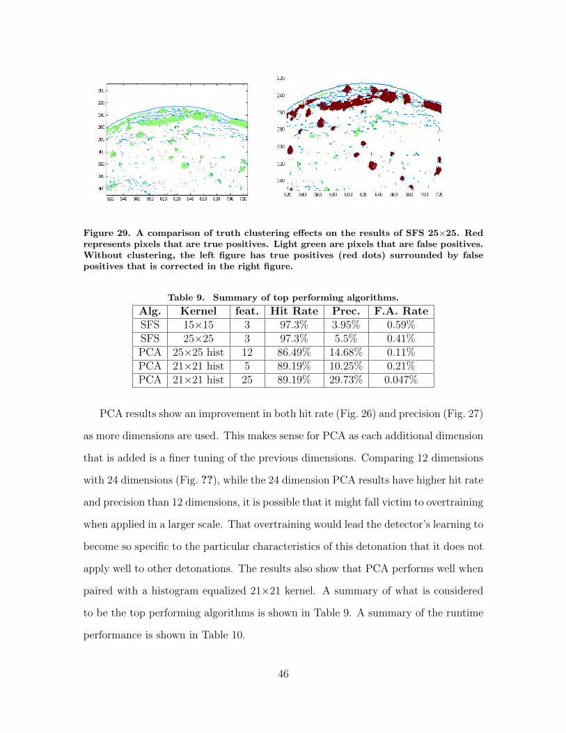
Figure 29. A comparison of truth clustering effects on the results of SFS 25×25. Redrepresents pixels that are true positives. Light green are pixels that are false positives.Without clustering, the left figure has true positives (red dots) surrounded by falsepositives that is corrected in the right figure.

Table 9. Summary of top performing algorithms.

Alg. Kernel feat. Hit Rate Prec. F.A. RateSFS 15×15 3 97.3% 3.95% 0.59%SFS 25×25 3 97.3% 5.5% 0.41%PCA 25×25 hist 12 86.49% 14.68% 0.11%PCA 21×21 hist 5 89.19% 10.25% 0.21%PCA 21×21 hist 25 89.19% 29.73% 0.047%

PCA results show an improvement in both hit rate (Fig. 26) and precision (Fig. 27)

as more dimensions are used. This makes sense for PCA as each additional dimension

that is added is a finer tuning of the previous dimensions. Comparing 12 dimensions

with 24 dimensions (Fig. ??), while the 24 dimension PCA results have higher hit rate

and precision than 12 dimensions, it is possible that it might fall victim to overtraining

when applied in a larger scale. That overtraining would lead the detector’s learning to

become so specific to the particular characteristics of this detonation that it does not

apply well to other detonations. The results also show that PCA performs well when

paired with a histogram equalized 21×21 kernel. A summary of what is considered

to be the top performing algorithms is shown in Table 9. A summary of the runtime

performance is shown in Table 10.

46

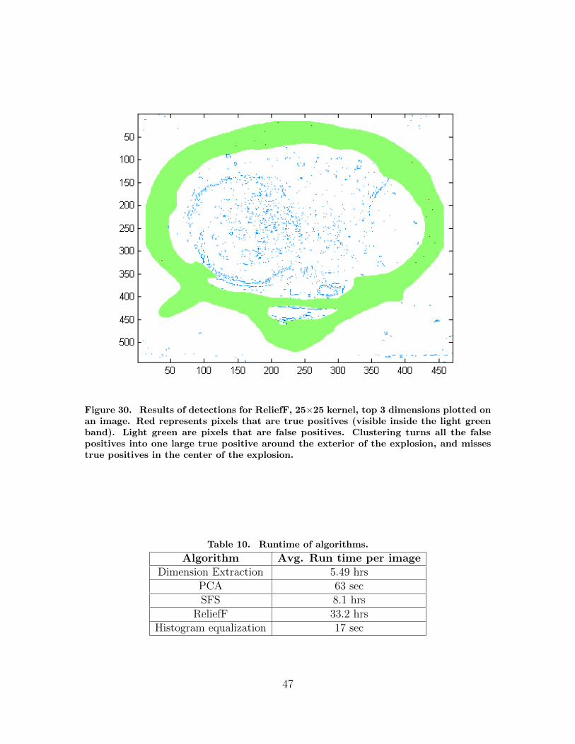
Figure 30. Results of detections for ReliefF, 25×25 kernel, top 3 dimensions plotted onan image. Red represents pixels that are true positives (visible inside the light greenband). Light green are pixels that are false positives. Clustering turns all the falsepositives into one large true positive around the exterior of the explosion, and missestrue positives in the center of the explosion.

Table 10. Runtime of algorithms.

Algorithm Avg. Run time per imageDimension Extraction 5.49 hrs

PCA 63 secSFS 8.1 hrs

ReliefF 33.2 hrsHistogram equalization 17 sec

47

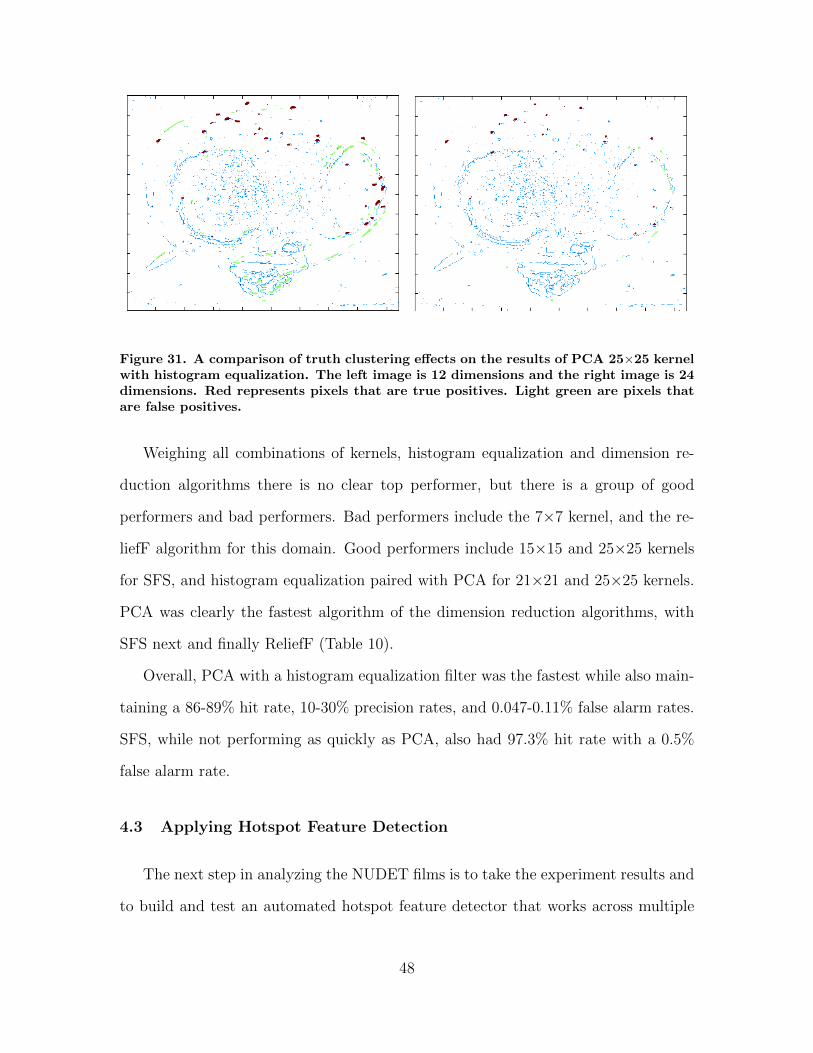
Figure 31. A comparison of truth clustering effects on the results of PCA 25×25 kernelwith histogram equalization. The left image is 12 dimensions and the right image is 24dimensions. Red represents pixels that are true positives. Light green are pixels thatare false positives.

Weighing all combinations of kernels, histogram equalization and dimension re-

duction algorithms there is no clear top performer, but there is a group of good

performers and bad performers. Bad performers include the 7×7 kernel, and the re-

liefF algorithm for this domain. Good performers include 15×15 and 25×25 kernels

for SFS, and histogram equalization paired with PCA for 21×21 and 25×25 kernels.

PCA was clearly the fastest algorithm of the dimension reduction algorithms, with

SFS next and finally ReliefF (Table 10).

Overall, PCA with a histogram equalization filter was the fastest while also main-

taining a 86-89% hit rate, 10-30% precision rates, and 0.047-0.11% false alarm rates.

SFS, while not performing as quickly as PCA, also had 97.3% hit rate with a 0.5%

false alarm rate.

4.3 Applying Hotspot Feature Detection

The next step in analyzing the NUDET films is to take the experiment results and

to build and test an automated hotspot feature detector that works across multiple

48

detonations. The results indicated that the best dimension of the 300 dimensions

studied was a 21×21 pixel kernel that took the average intensity of the center 3×3

pixel area and subtracted it from a 3 pixel border around the edge of the kernel. This

dimension determined which locations of the image had the highest relative intensities

to the area immediately around it. A hotspot detector was built using this dimension

and detections for a hotspot were considered present when the dimensions value was

larger than a threshold of the average intensity of the image + 2 standard deviations

of the intensity of the overall image. The results of this simplified hotspot detector

were then clustered based on whether they were adjacent to other positive detections

and catalogued. Information about the hotspot cluster was further derived based on

the cluster’s size to include its width in the x- and y-direction, its center, and the total

number of pixels in the cluster. Clusters that were too small (less than 10 pixels) or

too large (greater than 100 pixels) were discarded, and those that were not balanced

in x- and y-directions in span (within a 0.5 aspect ratio) were also discarded.

To determine the accuracy of this new approach to detecting hotspots, it was

tested against six detonations (Grable, Climax, Boltzmann, MET, Turk, and Tesla),

using at least two different viewpoints for each detonation, and 12 images for each

detonation. Images selected from a detonation were balanced evenly between when

detection was known to be difficult (when they are first visible in the detonation se-

quencing) and when it was suspected to be easiest (during tmin when the ambient light

is lowest and the hotspots are most pronounced). Seventy-two images were analyzed

in all, and the range of detonations included airdropped detonations and tower-based

detonations. Statistics were collected to determine the hit rate (sensitivity), precision

and false positive rate. Fig. 32 shows an example of results for the Boltzmann deto-

nation. The hit rate for all the detonations was measured at 71.95%, with a 86.03%

precision and a 0.015% false positive rate. The false positive rate was extremely low

49

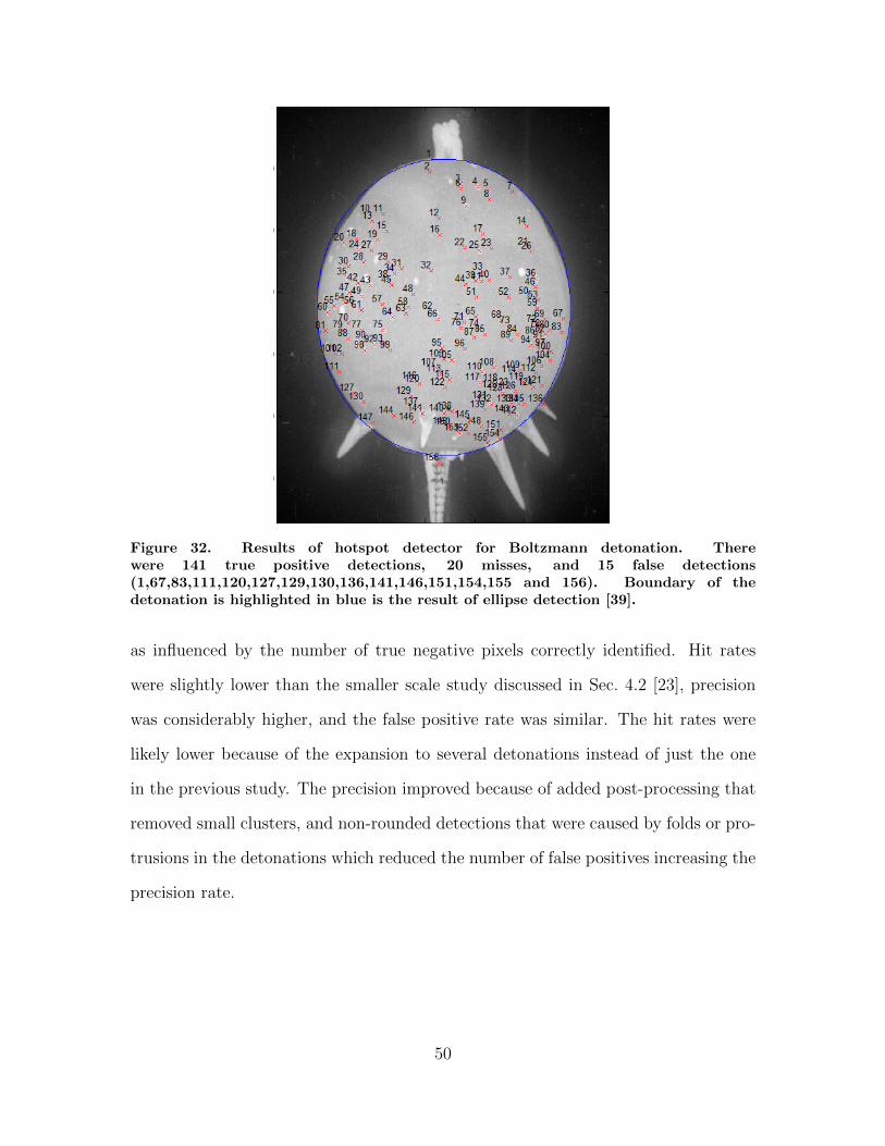
Figure 32. Results of hotspot detector for Boltzmann detonation. Therewere 141 true positive detections, 20 misses, and 15 false detections(1,67,83,111,120,127,129,130,136,141,146,151,154,155 and 156). Boundary of thedetonation is highlighted in blue is the result of ellipse detection [39].

as influenced by the number of true negative pixels correctly identified. Hit rates

were slightly lower than the smaller scale study discussed in Sec. 4.2 [23], precision

was considerably higher, and the false positive rate was similar. The hit rates were

likely lower because of the expansion to several detonations instead of just the one

in the previous study. The precision improved because of added post-processing that

removed small clusters, and non-rounded detections that were caused by folds or pro-

trusions in the detonations which reduced the number of false positives increasing the

precision rate.

50

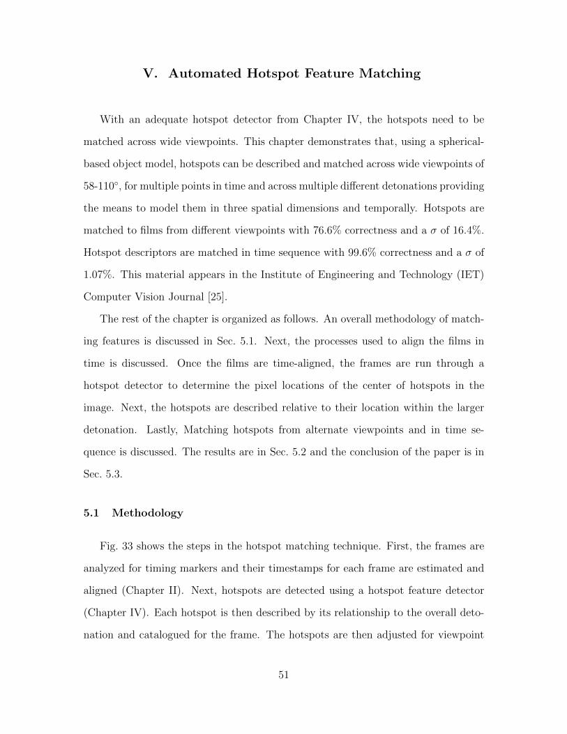
V. Automated Hotspot Feature Matching

With an adequate hotspot detector from Chapter IV, the hotspots need to be

matched across wide viewpoints. This chapter demonstrates that, using a spherical-

based object model, hotspots can be described and matched across wide viewpoints of

58-110◦, for multiple points in time and across multiple different detonations providing

the means to model them in three spatial dimensions and temporally. Hotspots are

matched to films from different viewpoints with 76.6% correctness and a σ of 16.4%.

Hotspot descriptors are matched in time sequence with 99.6% correctness and a σ of

1.07%. This material appears in the Institute of Engineering and Technology (IET)

Computer Vision Journal [25].

The rest of the chapter is organized as follows. An overall methodology of match-

ing features is discussed in Sec. 5.1. Next, the processes used to align the films in

time is discussed. Once the films are time-aligned, the frames are run through a

hotspot detector to determine the pixel locations of the center of hotspots in the

image. Next, the hotspots are described relative to their location within the larger

detonation. Lastly, Matching hotspots from alternate viewpoints and in time se-

quence is discussed. The results are in Sec. 5.2 and the conclusion of the paper is in

Sec. 5.3.

5.1 Methodology

Fig. 33 shows the steps in the hotspot matching technique. First, the frames are

analyzed for timing markers and their timestamps for each frame are estimated and

aligned (Chapter II). Next, hotspots are detected using a hotspot feature detector

(Chapter IV). Each hotspot is then described by its relationship to the overall deto-

nation and catalogued for the frame. The hotspots are then adjusted for viewpoint

51

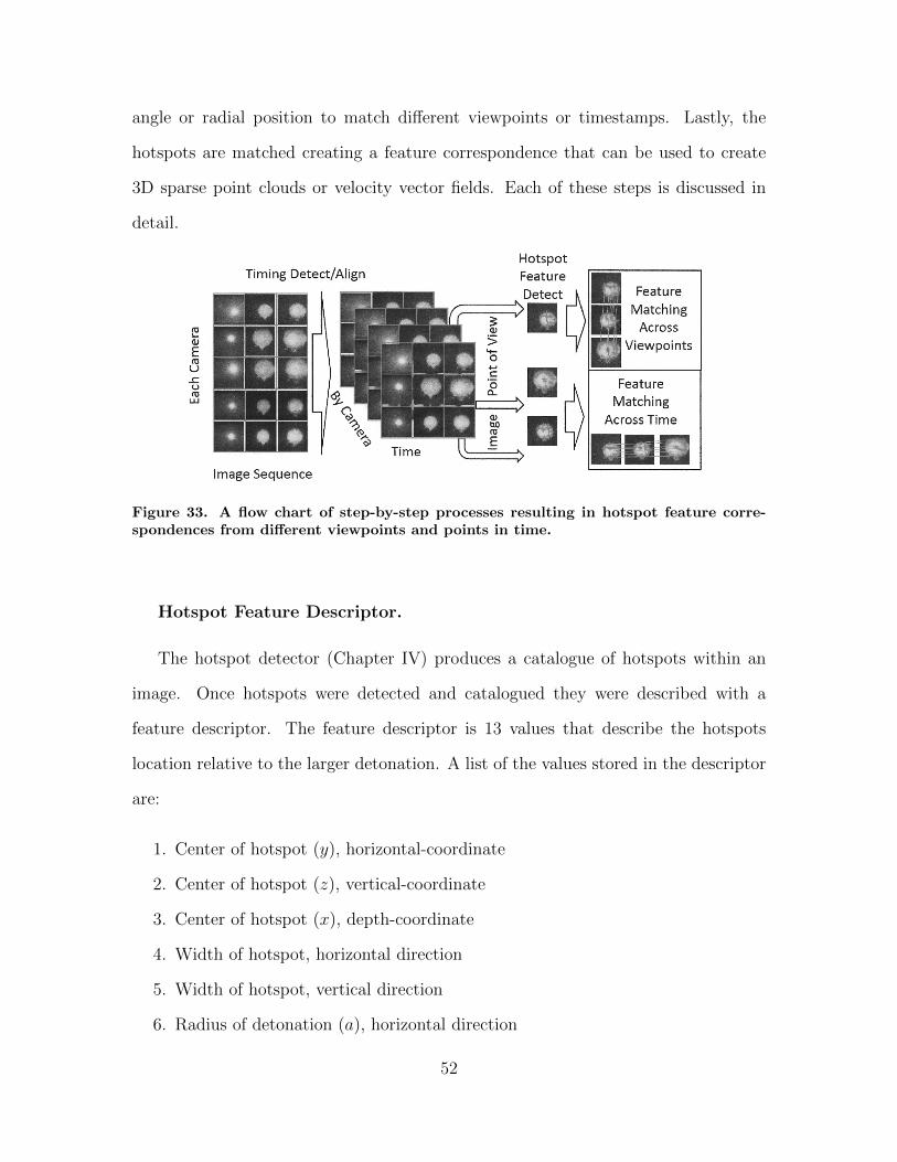
angle or radial position to match different viewpoints or timestamps. Lastly, the

hotspots are matched creating a feature correspondence that can be used to create

3D sparse point clouds or velocity vector fields. Each of these steps is discussed in

detail.

Figure 33. A flow chart of step-by-step processes resulting in hotspot feature corre-spondences from different viewpoints and points in time.

Hotspot Feature Descriptor.

The hotspot detector (Chapter IV) produces a catalogue of hotspots within an

image. Once hotspots were detected and catalogued they were described with a

feature descriptor. The feature descriptor is 13 values that describe the hotspots

location relative to the larger detonation. A list of the values stored in the descriptor

are:

1. Center of hotspot (y), horizontal-coordinate

2. Center of hotspot (z), vertical-coordinate

3. Center of hotspot (x), depth-coordinate

4. Width of hotspot, horizontal direction

5. Width of hotspot, vertical direction

6. Radius of detonation (a), horizontal direction

52

7. Radius of detonation (b), vertical direction

8. Inclination coordinate (θ) of hotspot relative to center of detonation

9. Azimuth coordinate (ϕ) of hotspot relative to center of detonation

10. Radius coordinate (r) of hotspot relative to center of detonation

11. Center of detonation (yc), horizontal-coordinate

12. Center of detonation (zc), vertical-coordinate

13. Number of pixels in hotspot

Several of the values (3, 6-12) are based on the overall detonation. To acquire

that information, an ellipse detector [39] was applied to the detonation. The ellipse

detection is highlighted in Fig. 32. Using the ellipse, an assumption is made that

the detonation is an ellipsoid in 3D with equal depth and horizontal dimensions but

potentially differing vertical dimensions. Using the location of the hotspot relative

to the larger detonation, the horizontal and vertical coordinates are translated into

polar coordinates. For polar coordinates, the reference frame assigned z to the vertical

axis, y to the horizontal axis, and x to the depth axis. Eq. 6 through Eq. 9 show

the equations for calculating the polar coordinates with a representing the radius of

the larger detonation in the horizontal direction, and b representing the radius in the

vertical direction. The center of the detonation is assumed to be at zero in the depth

direction.

x =

√a2 − (y − yc)2 − [

a2(z − zc)2

b2] (6)

r =√x2 + (y − yc)2 + (z − zc)2 (7)

θ = cos−1(z − zcr

) (8)

ϕ = tan−1(y − ycx

) (9)

53

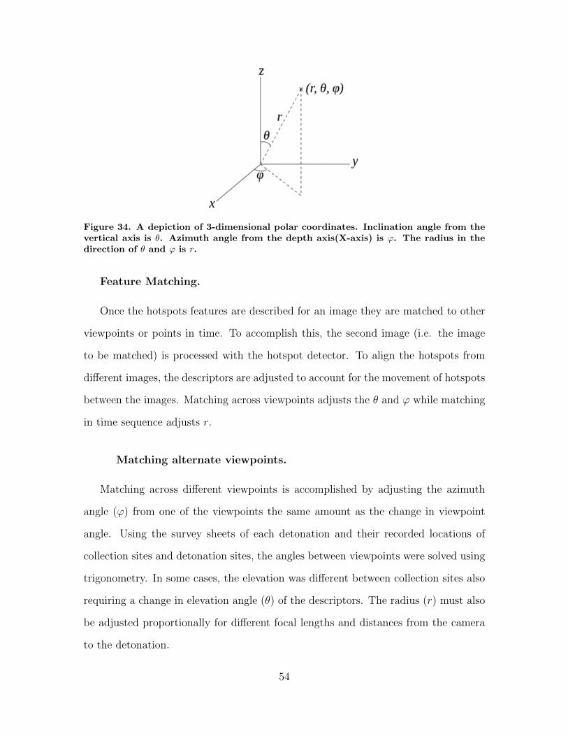
Figure 34. A depiction of 3-dimensional polar coordinates. Inclination angle from thevertical axis is θ. Azimuth angle from the depth axis(X-axis) is ϕ. The radius in thedirection of θ and ϕ is r.

Feature Matching.

Once the hotspots features are described for an image they are matched to other

viewpoints or points in time. To accomplish this, the second image (i.e. the image

to be matched) is processed with the hotspot detector. To align the hotspots from

different images, the descriptors are adjusted to account for the movement of hotspots

between the images. Matching across viewpoints adjusts the θ and ϕ while matching

in time sequence adjusts r.

Matching alternate viewpoints.

Matching across different viewpoints is accomplished by adjusting the azimuth

angle (ϕ) from one of the viewpoints the same amount as the change in viewpoint

angle. Using the survey sheets of each detonation and their recorded locations of

collection sites and detonation sites, the angles between viewpoints were solved using

trigonometry. In some cases, the elevation was different between collection sites also

requiring a change in elevation angle (θ) of the descriptors. The radius (r) must also

be adjusted proportionally for different focal lengths and distances from the camera

to the detonation.

54

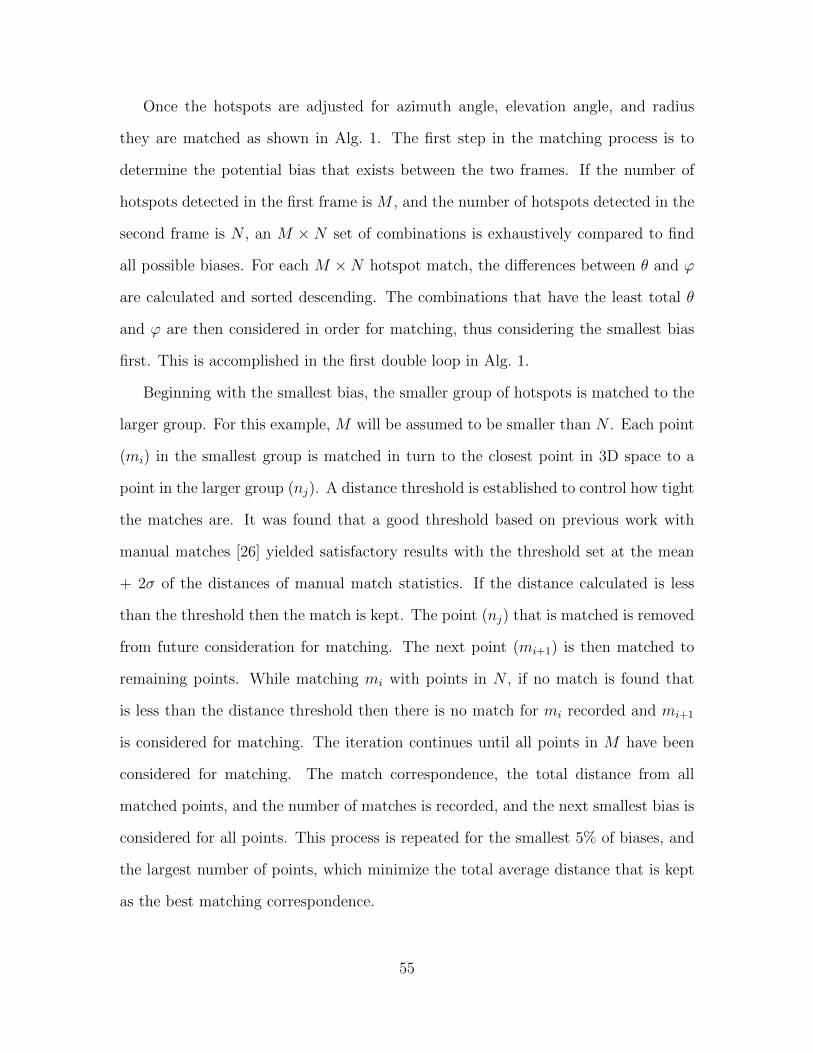
Once the hotspots are adjusted for azimuth angle, elevation angle, and radius

they are matched as shown in Alg. 1. The first step in the matching process is to

determine the potential bias that exists between the two frames. If the number of

hotspots detected in the first frame is M , and the number of hotspots detected in the

second frame is N , an M × N set of combinations is exhaustively compared to find

all possible biases. For each M ×N hotspot match, the differences between θ and ϕ

are calculated and sorted descending. The combinations that have the least total θ

and ϕ are then considered in order for matching, thus considering the smallest bias

first. This is accomplished in the first double loop in Alg. 1.

Beginning with the smallest bias, the smaller group of hotspots is matched to the

larger group. For this example, M will be assumed to be smaller than N . Each point

(mi) in the smallest group is matched in turn to the closest point in 3D space to a

point in the larger group (nj). A distance threshold is established to control how tight

the matches are. It was found that a good threshold based on previous work with

manual matches [26] yielded satisfactory results with the threshold set at the mean

+ 2σ of the distances of manual match statistics. If the distance calculated is less

than the threshold then the match is kept. The point (nj) that is matched is removed

from future consideration for matching. The next point (mi+1) is then matched to

remaining points. While matching mi with points in N , if no match is found that

is less than the distance threshold then there is no match for mi recorded and mi+1

is considered for matching. The iteration continues until all points in M have been

considered for matching. The match correspondence, the total distance from all

matched points, and the number of matches is recorded, and the next smallest bias is

considered for all points. This process is repeated for the smallest 5% of biases, and

the largest number of points, which minimize the total average distance that is kept

as the best matching correspondence.

55

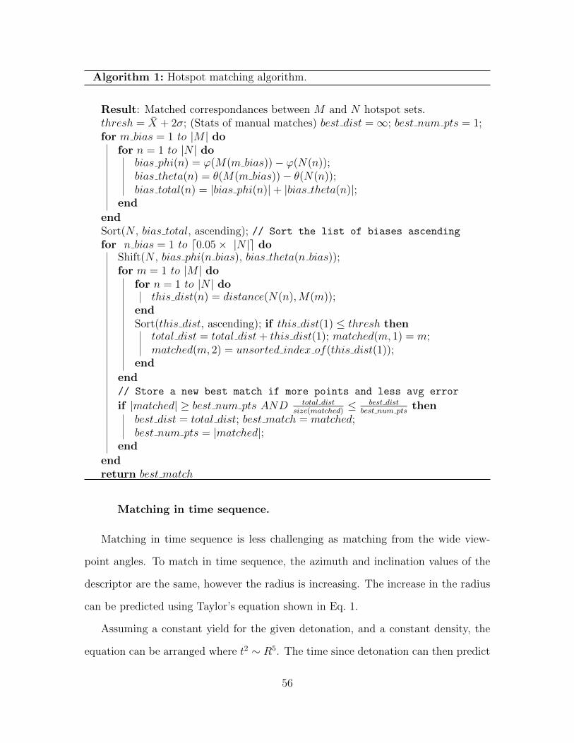
Algorithm 1: Hotspot matching algorithm.

Result: Matched correspondances between M and N hotspot sets.thresh = X̄ + 2σ; (Stats of manual matches) best dist =∞; best num pts = 1;for m bias = 1 to |M | do

for n = 1 to |N | dobias phi(n) = ϕ(M(m bias))− ϕ(N(n));bias theta(n) = θ(M(m bias))− θ(N(n));bias total(n) = |bias phi(n)|+ |bias theta(n)|;

end

endSort(N , bias total, ascending); // Sort the list of biases ascending

for n bias = 1 to d0.05× |N |e doShift(N , bias phi(n bias), bias theta(n bias));for m = 1 to |M | do

for n = 1 to |N | dothis dist(n) = distance(N(n),M(m));

endSort(this dist, ascending); if this dist(1) ≤ thresh then

total dist = total dist+ this dist(1); matched(m, 1) = m;matched(m, 2) = unsorted index of(this dist(1));

end

end// Store a new best match if more points and less avg error

if |matched| ≥ best num pts AND total distsize(matched)

≤ best distbest num pts

thenbest dist = total dist; best match = matched;best num pts = |matched|;

end

endreturn best match

Matching in time sequence.

Matching in time sequence is less challenging as matching from the wide view-

point angles. To match in time sequence, the azimuth and inclination values of the

descriptor are the same, however the radius is increasing. The increase in the radius

can be predicted using Taylor’s equation shown in Eq. 1.

Assuming a constant yield for the given detonation, and a constant density, the

equation can be arranged where t2 ∼ R5. The time since detonation can then predict

56

the radius, and a ∆t in small increments in t can be used to find a ∆R. Since the

time since detonation is already estimated (see Sec. 2.4), it can be used to predict

the change in radius from frame to frame.

The algorithm for matching in time sequence works exactly like that of matching

alternate viewpoints (Alg. 1). The difference is the inputs are the hotspots from the

original frame, adjusted by the ∆R and the hotspots from next frame in time sequence.

The hotspots are only adjusted in radius, and not in azimuth (ϕ) or inclination (θ).

5.2 Results

At the time of testing, only twelve films were digitized and available for testing.

Four of the twelve films did not show discernible hotspots. Of the eight remaining

films, six had multiple films from the same viewpoints, which significantly increased

the number of time aligned frames making them more useful for testing. The accu-

racy of matching alternate viewpoints was tested using the six detonations listed in

Table 11. The accuracy was determined by verifying the correctness of each matched

correspondence by visual inspection. Since the model that is used to describe and

rotate hotspots is based on polar coordinates, the airdrop detonations were expected

to perform better because they are more spherical, and have fewer disparities with

that model. The tower detonations were included to challenge the model to see how

accurate matching would be with non-elliptical shaped detonations and detonations

with cone protrusions. The detonations listed in Table 11 are ordered from most

spherical to least spherical. A variety of viewpoint angles were tested ranging from

58◦ to almost 110◦.

57

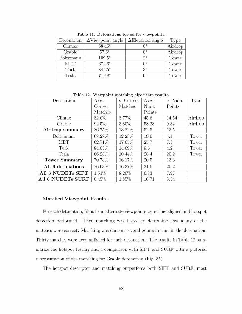
Table 11. Detonations tested for viewpoints.

Detonation ∆Viewpoint angle ∆Elevation angle TypeClimax 68.46◦ 0◦ AirdropGrable 57.6◦ 0◦ Airdrop

Boltzmann 109.5◦ 2◦ TowerMET 67.46◦ 0◦ TowerTurk 84.25◦ 3◦ TowerTesla 71.48◦ 0◦ Tower

Table 12. Viewpoint matching algorithm results.

Detonation Avg.CorrectMatches

σ CorrectMatches

Avg.Num.Points

σ Num.Points

Type

Climax 82.6% 8.77% 45.6 14.54 AirdropGrable 92.5% 3.80% 58.23 9.32 Airdrop

Airdrop summary 86.75% 13.22% 52.5 13.5

Boltzmann 68.28% 12.23% 19.6 5.1 TowerMET 62.71% 17.65% 25.7 7.3 TowerTurk 84.05% 14.69% 9.6 4.2 TowerTesla 66.23% 10.44% 28.4 20.2 Tower

Tower Summary 70.73% 16.17% 20.5 13.3

All 6 detonations 76.63% 16.37% 31.6 20.2

All 6 NUDETs SIFT 1.51% 8.20% 6.83 7.97All 6 NUDETs SURF 0.45% 1.85% 16.71 5.54

Matched Viewpoint Results.

For each detonation, films from alternate viewpoints were time aligned and hotspot

detection performed. Then matching was tested to determine how many of the

matches were correct. Matching was done at several points in time in the detonation.

Thirty matches were accomplished for each detonation. The results in Table 12 sum-

marize the hotspot testing and a comparison with SIFT and SURF with a pictorial

representation of the matching for Grable detonation (Fig. 35).

The hotspot descriptor and matching outperfoms both SIFT and SURF, most

58

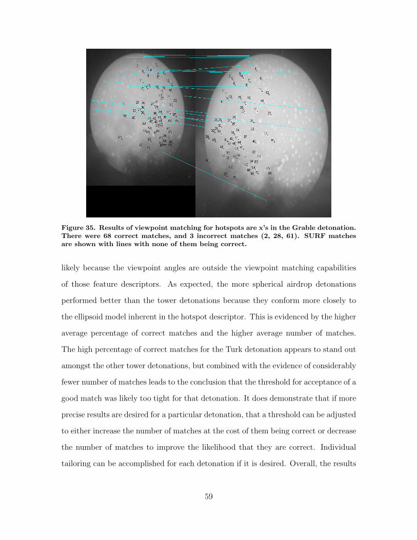
Figure 35. Results of viewpoint matching for hotspots are x’s in the Grable detonation.There were 68 correct matches, and 3 incorrect matches (2, 28, 61). SURF matchesare shown with lines with none of them being correct.

likely because the viewpoint angles are outside the viewpoint matching capabilities

of those feature descriptors. As expected, the more spherical airdrop detonations

performed better than the tower detonations because they conform more closely to

the ellipsoid model inherent in the hotspot descriptor. This is evidenced by the higher

average percentage of correct matches and the higher average number of matches.

The high percentage of correct matches for the Turk detonation appears to stand out

amongst the other tower detonations, but combined with the evidence of considerably

fewer number of matches leads to the conclusion that the threshold for acceptance of a

good match was likely too tight for that detonation. It does demonstrate that if more

precise results are desired for a particular detonation, that a threshold can be adjusted

to either increase the number of matches at the cost of them being correct or decrease

the number of matches to improve the likelihood that they are correct. Individual

tailoring can be accomplished for each detonation if it is desired. Overall, the results

59

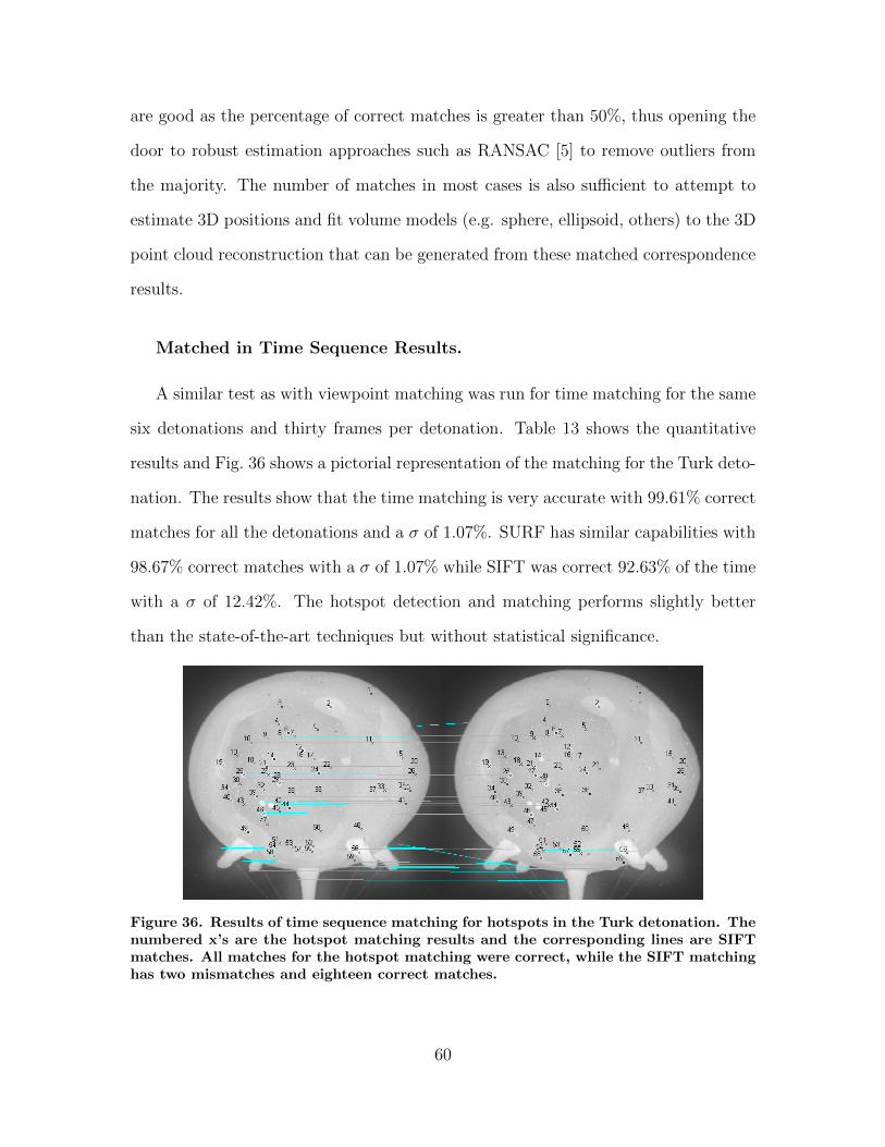
are good as the percentage of correct matches is greater than 50%, thus opening the

door to robust estimation approaches such as RANSAC [5] to remove outliers from

the majority. The number of matches in most cases is also sufficient to attempt to

estimate 3D positions and fit volume models (e.g. sphere, ellipsoid, others) to the 3D

point cloud reconstruction that can be generated from these matched correspondence

results.

Matched in Time Sequence Results.

A similar test as with viewpoint matching was run for time matching for the same

six detonations and thirty frames per detonation. Table 13 shows the quantitative

results and Fig. 36 shows a pictorial representation of the matching for the Turk deto-

nation. The results show that the time matching is very accurate with 99.61% correct

matches for all the detonations and a σ of 1.07%. SURF has similar capabilities with

98.67% correct matches with a σ of 1.07% while SIFT was correct 92.63% of the time

with a σ of 12.42%. The hotspot detection and matching performs slightly better

than the state-of-the-art techniques but without statistical significance.

Figure 36. Results of time sequence matching for hotspots in the Turk detonation. Thenumbered x’s are the hotspot matching results and the corresponding lines are SIFTmatches. All matches for the hotspot matching were correct, while the SIFT matchinghas two mismatches and eighteen correct matches.

60

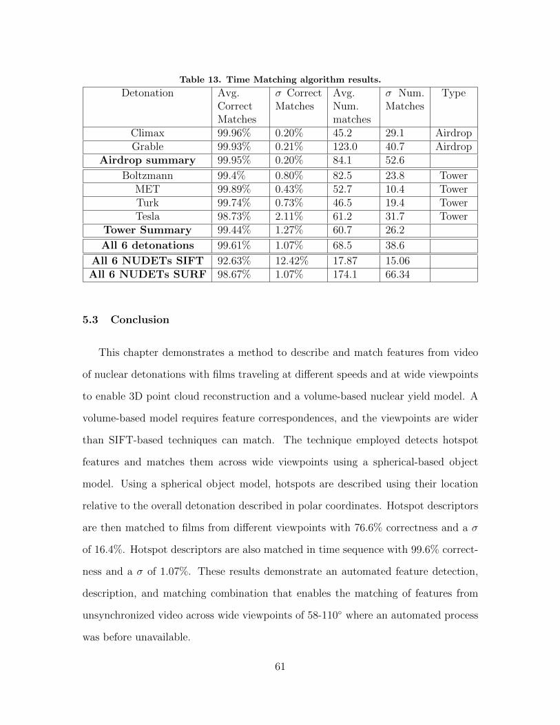
Table 13. Time Matching algorithm results.

Detonation Avg.CorrectMatches

σ CorrectMatches

Avg.Num.matches

σ Num.Matches

Type

Climax 99.96% 0.20% 45.2 29.1 AirdropGrable 99.93% 0.21% 123.0 40.7 Airdrop

Airdrop summary 99.95% 0.20% 84.1 52.6

Boltzmann 99.4% 0.80% 82.5 23.8 TowerMET 99.89% 0.43% 52.7 10.4 TowerTurk 99.74% 0.73% 46.5 19.4 TowerTesla 98.73% 2.11% 61.2 31.7 Tower

Tower Summary 99.44% 1.27% 60.7 26.2

All 6 detonations 99.61% 1.07% 68.5 38.6

All 6 NUDETs SIFT 92.63% 12.42% 17.87 15.06All 6 NUDETs SURF 98.67% 1.07% 174.1 66.34

5.3 Conclusion

This chapter demonstrates a method to describe and match features from video

of nuclear detonations with films traveling at different speeds and at wide viewpoints

to enable 3D point cloud reconstruction and a volume-based nuclear yield model. A

volume-based model requires feature correspondences, and the viewpoints are wider

than SIFT-based techniques can match. The technique employed detects hotspot

features and matches them across wide viewpoints using a spherical-based object

model. Using a spherical object model, hotspots are described using their location

relative to the overall detonation described in polar coordinates. Hotspot descriptors

are then matched to films from different viewpoints with 76.6% correctness and a σ

of 16.4%. Hotspot descriptors are also matched in time sequence with 99.6% correct-

ness and a σ of 1.07%. These results demonstrate an automated feature detection,

description, and matching combination that enables the matching of features from

unsynchronized video across wide viewpoints of 58-110◦ where an automated process

was before unavailable.

61

This chapter demonstrates that a spherical model can be used effectively as the

basis for a feature descriptor for ellipsoid-like objects. This allows the comparison

across wider viewpoints without the need of Harris [7] corners.

Next, the matched correspondences were used to generate 3D point clouds of

differing viewpoints and tracking them through time. The discussion about how

accurate the points in the point cloud continues in Chapter VI. Point locations were

tracked in time as well as volumes inferred from the point clouds. The discussion

about volumes continues in Chapter VII.

62

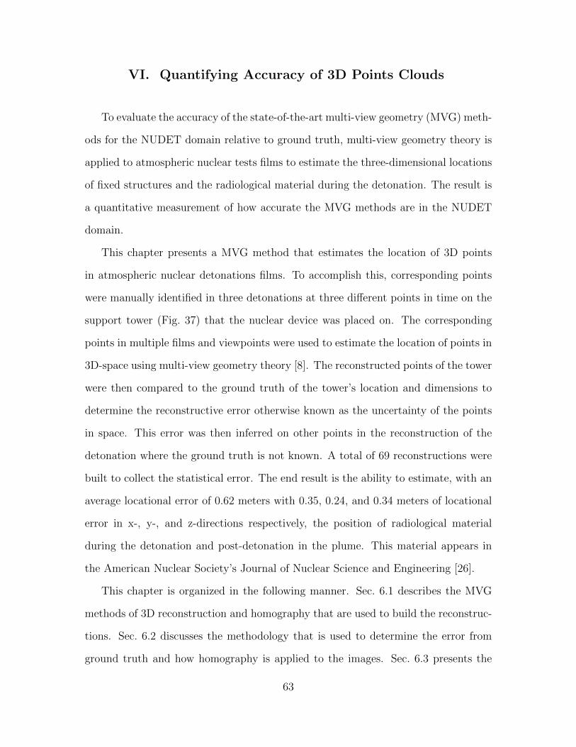
VI. Quantifying Accuracy of 3D Points Clouds

To evaluate the accuracy of the state-of-the-art multi-view geometry (MVG) meth-

ods for the NUDET domain relative to ground truth, multi-view geometry theory is

applied to atmospheric nuclear tests films to estimate the three-dimensional locations

of fixed structures and the radiological material during the detonation. The result is

a quantitative measurement of how accurate the MVG methods are in the NUDET

domain.

This chapter presents a MVG method that estimates the location of 3D points

in atmospheric nuclear detonations films. To accomplish this, corresponding points

were manually identified in three detonations at three different points in time on the

support tower (Fig. 37) that the nuclear device was placed on. The corresponding

points in multiple films and viewpoints were used to estimate the location of points in

3D-space using multi-view geometry theory [8]. The reconstructed points of the tower

were then compared to the ground truth of the tower’s location and dimensions to

determine the reconstructive error otherwise known as the uncertainty of the points

in space. This error was then inferred on other points in the reconstruction of the

detonation where the ground truth is not known. A total of 69 reconstructions were

built to collect the statistical error. The end result is the ability to estimate, with an

average locational error of 0.62 meters with 0.35, 0.24, and 0.34 meters of locational

error in x-, y-, and z-directions respectively, the position of radiological material

during the detonation and post-detonation in the plume. This material appears in

the American Nuclear Society’s Journal of Nuclear Science and Engineering [26].

This chapter is organized in the following manner. Sec. 6.1 describes the MVG

methods of 3D reconstruction and homography that are used to build the reconstruc-

tions. Sec. 6.2 discusses the methodology that is used to determine the error from

ground truth and how homography is applied to the images. Sec. 6.3 presents the

63

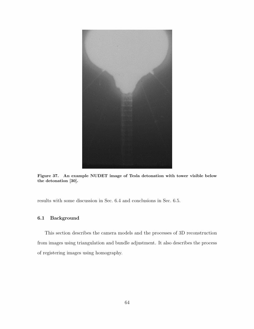
Figure 37. An example NUDET image of Tesla detonation with tower visible belowthe detonation [30].

results with some discussion in Sec. 6.4 and conclusions in Sec. 6.5.

6.1 Background

This section describes the camera models and the processes of 3D reconstruction

from images using triangulation and bundle adjustment. It also describes the process

of registering images using homography.

64

Homogeneous coordinates.

In MVG, homogeneous coordinates are used so that points in the real world can

be related to points in multiple images more easily [8]. A point in Euclidean 3-space

is represented by an ordered pair of real numbers (x, y, z). To make the coordinate

homogeneous, a fourth digit is added to create the homogeneous coordinate definition

that (x, y, z) = (x, y, z, 1). The definition also implies that (x, y, z) = (x, y, z, 1) =

(2x, 2y, 2z, 2) = (kx, ky, kz, k) for any non-zero value of k. The parameter k is then

sometimes referred to as a scaling factor that facilities relating images together that

have different scale.

Furthermore, we can use homogeneous coordinates to then define projective space.

The Euclidean space Rn can be extended to projective space Pn by representing points

as homogeneous vectors [8].

Camera Models.

To apply multi-view geometry to the NUDET films, information recorded at the

time of detonation is interpreted using camera models. This section details the theory

of the pinhole camera, which underpins the finite projective camera model. The finite

projective camera is then used in Sec. 6.2 with information from the NUDET films

with triangulation and bundle adjustment to create the 3D structure of the NUDET

with points on the NUDET tower.

Pinhole Camera.

The pinhole camera model is a basic model of how images are captured by a

camera. Fig. 38 shows a depiction of the pinhole camera model. Letting X represent

a point in the 3-dimensional world represented by X = (X, Y, Z)T ∈ R3 in Euclidean

space. The camera center (optical center), C is located at the origin of this Euclidean

65

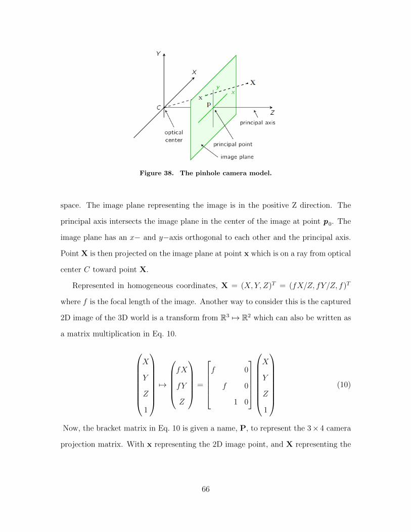
Figure 38. The pinhole camera model.

space. The image plane representing the image is in the positive Z direction. The

principal axis intersects the image plane in the center of the image at point p0. The

image plane has an x− and y−axis orthogonal to each other and the principal axis.

Point X is then projected on the image plane at point x which is on a ray from optical

center C toward point X.

Represented in homogeneous coordinates, X = (X, Y, Z)T = (fX/Z, fY/Z, f)T

where f is the focal length of the image. Another way to consider this is the captured

2D image of the 3D world is a transform from R3 7→ R2 which can also be written as

a matrix multiplication in Eq. 10.

X

Y

Z

1

7→

fX

fY

Z

=

f 0

f 0

1 0

X

Y

Z

1

(10)

Now, the bracket matrix in Eq. 10 is given a name, P, to represent the 3× 4 camera

projection matrix. With x representing the 2D image point, and X representing the

66

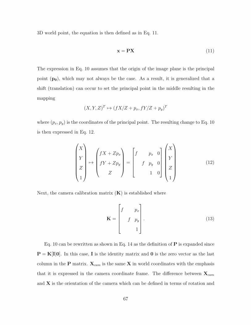
3D world point, the equation is then defined as in Eq. 11.

x = PX (11)

The expression in Eq. 10 assumes that the origin of the image plane is the principal

point (p0), which may not always be the case. As a result, it is generalized that a

shift (translation) can occur to set the principal point in the middle resulting in the

mapping

(X, Y, Z)T 7→ (fX/Z + px, fY/Z + py)T

where (px, py) is the coordinates of the principal point. The resulting change to Eq. 10

is then expressed in Eq. 12.

X

Y

Z

1

7→

fX + Zpx

fY + Zpy

Z

=

f px 0

f py 0

1 0

X

Y

Z

1

(12)

Next, the camera calibration matrix (K) is established where

K =

f px

f py

1

. (13)

Eq. 10 can be rewritten as shown in Eq. 14 as the definition of P is expanded since

P = K[I|0]. In this case, I is the identity matrix and 0 is the zero vector as the last

column in the P matrix. Xcam is the same X in world coordinates with the emphasis

that it is expressed in the camera coordinate frame. The difference between Xcam

and X is the orientation of the camera which can be defined in terms of rotation and

67

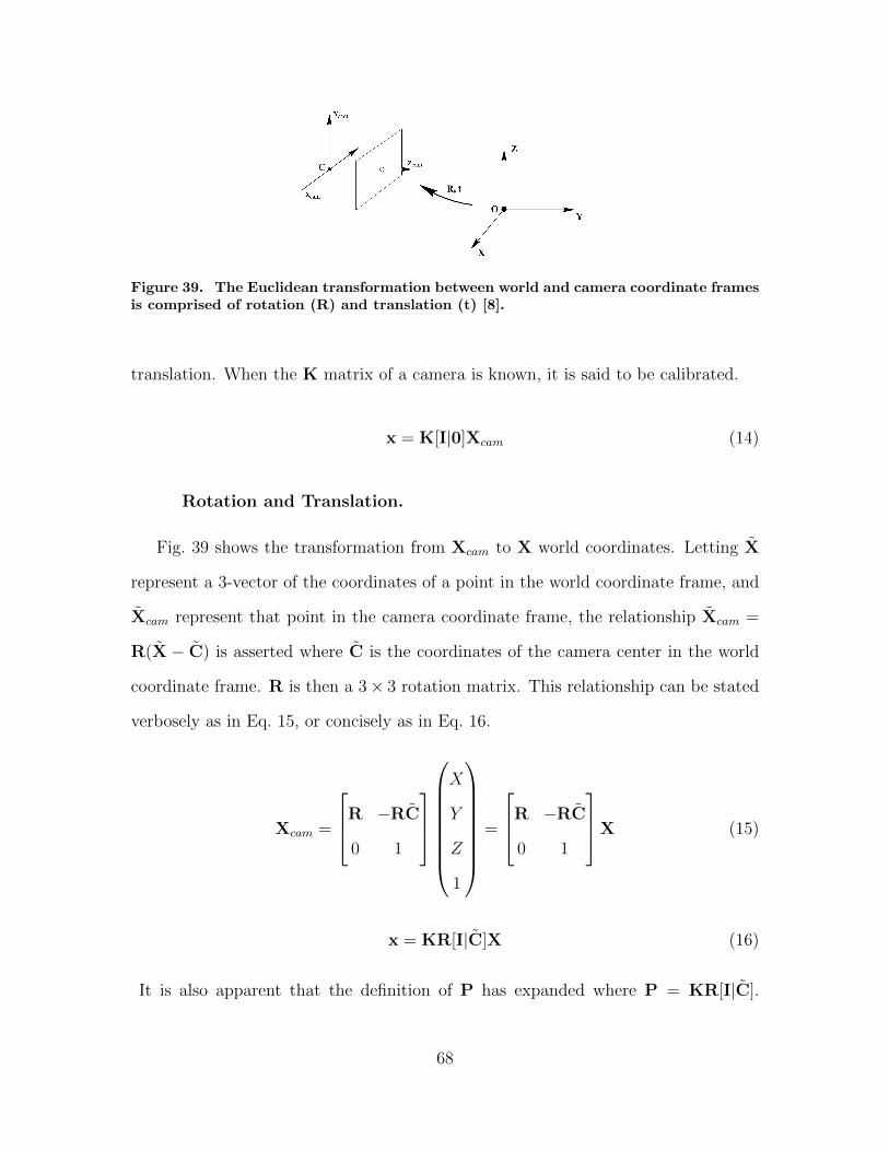
Figure 39. The Euclidean transformation between world and camera coordinate framesis comprised of rotation (R) and translation (t) [8].

translation. When the K matrix of a camera is known, it is said to be calibrated.

x = K[I|0]Xcam (14)

Rotation and Translation.

Fig. 39 shows the transformation from Xcam to X world coordinates. Letting X̃

represent a 3-vector of the coordinates of a point in the world coordinate frame, and

X̃cam represent that point in the camera coordinate frame, the relationship X̃cam =

R(X̃ − C̃) is asserted where C̃ is the coordinates of the camera center in the world

coordinate frame. R is then a 3× 3 rotation matrix. This relationship can be stated

verbosely as in Eq. 15, or concisely as in Eq. 16.

Xcam =

R −RC̃

0 1

X

Y

Z

1

=

R −RC̃

0 1

X (15)

x = KR[I|C̃]X (16)

It is also apparent that the definition of P has expanded where P = KR[I|C̃].

68

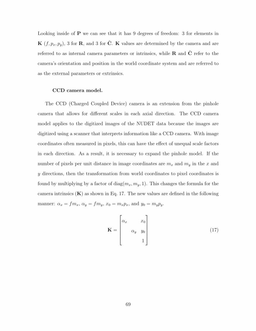
Looking inside of P we can see that it has 9 degrees of freedom: 3 for elements in

K (f, px, py), 3 for R, and 3 for C̃. K values are determined by the camera and are

referred to as internal camera parameters or intrinsics, while R and C̃ refer to the

camera’s orientation and position in the world coordinate system and are referred to

as the external parameters or extrinsics.

CCD camera model.

The CCD (Charged Coupled Device) camera is an extension from the pinhole

camera that allows for different scales in each axial direction. The CCD camera

model applies to the digitized images of the NUDET data because the images are

digitized using a scanner that interprets information like a CCD camera. With image

coordinates often measured in pixels, this can have the effect of unequal scale factors

in each direction. As a result, it is necessary to expand the pinhole model. If the

number of pixels per unit distance in image coordinates are mx and my in the x and

y directions, then the transformation from world coordinates to pixel coordinates is

found by multiplying by a factor of diag(mx,my, 1). This changes the formula for the

camera intrinsics (K) as shown in Eq. 17. The new values are defined in the following

manner: αx = fmx, αy = fmy, x0 = mxpx, and y0 = mypy.

K =

αx x0

αy y0

1

(17)

69

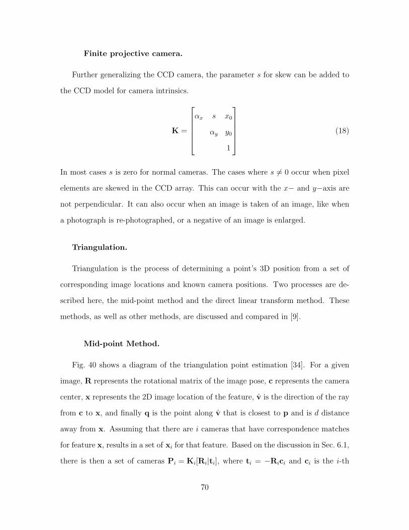
Finite projective camera.

Further generalizing the CCD camera, the parameter s for skew can be added to

the CCD model for camera intrinsics.

K =

αx s x0

αy y0

1

(18)

In most cases s is zero for normal cameras. The cases where s 6= 0 occur when pixel

elements are skewed in the CCD array. This can occur with the x− and y−axis are

not perpendicular. It can also occur when an image is taken of an image, like when

a photograph is re-photographed, or a negative of an image is enlarged.

Triangulation.

Triangulation is the process of determining a point’s 3D position from a set of

corresponding image locations and known camera positions. Two processes are de-

scribed here, the mid-point method and the direct linear transform method. These

methods, as well as other methods, are discussed and compared in [9].

Mid-point Method.

Fig. 40 shows a diagram of the triangulation point estimation [34]. For a given

image, R represents the rotational matrix of the image pose, c represents the camera

center, x represents the 2D image location of the feature, v̂ is the direction of the ray

from c to x, and finally q is the point along v̂ that is closest to p and is d distance

away from x. Assuming that there are i cameras that have correspondence matches

for feature x, results in a set of xi for that feature. Based on the discussion in Sec. 6.1,

there is then a set of cameras Pi = Ki[Ri|ti], where ti = −Rici and ci is the i-th

70

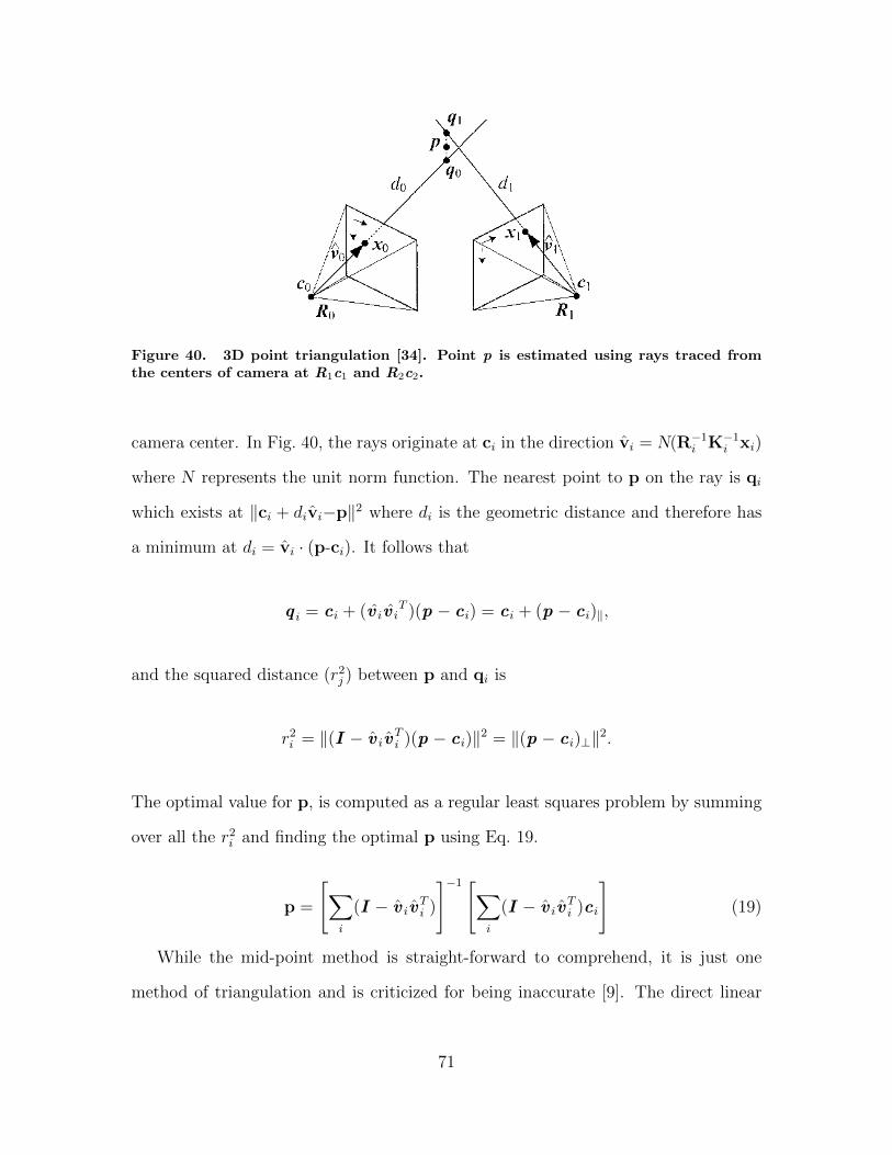
Figure 40. 3D point triangulation [34]. Point p is estimated using rays traced fromthe centers of camera at R1c1 and R2c2.

camera center. In Fig. 40, the rays originate at ci in the direction v̂i = N(R−1i K−1

i xi)

where N represents the unit norm function. The nearest point to p on the ray is qi

which exists at ‖ci + div̂i−p‖2 where di is the geometric distance and therefore has

a minimum at di = v̂i · (p-ci). It follows that

q i = ci + (v̂ iv̂ iT )(p − ci) = ci + (p − ci)‖,

and the squared distance (r2j ) between p and qi is

r2i = ‖(I − v̂ iv̂

Ti )(p − ci)‖2 = ‖(p − ci)⊥‖2.

The optimal value for p, is computed as a regular least squares problem by summing

over all the r2i and finding the optimal p using Eq. 19.

p =

[∑i

(I − v̂ iv̂Ti )

]−1 [∑i

(I − v̂ iv̂Ti )ci

](19)

While the mid-point method is straight-forward to comprehend, it is just one

method of triangulation and is criticized for being inaccurate [9]. The direct linear

71

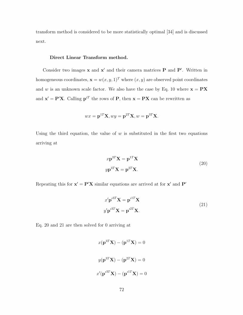
transform method is considered to be more statistically optimal [34] and is discussed

next.

Direct Linear Transform method.

Consider two images x and x′ and their camera matrices P and P′. Written in

homogeneous coordinates, x = w(x, y, 1)T where (x, y) are observed point coordinates

and w is an unknown scale factor. We also have the case by Eq. 10 where x = PX

and x′ = P′X. Calling piT the rows of P, then x = PX can be rewritten as

wx = p1TX, wy = p2TX, w = p3TX.

Using the third equation, the value of w is substituted in the first two equations

arriving at

xp3TX = p1TX

yp3TX = p2TX.

(20)

Repeating this for x′ = P′X similar equations are arrived at for x′ and P′

x′p′3TX = p′

1TX

y′p′3TX = p′

2TX.

(21)

Eq. 20 and 21 are then solved for 0 arriving at

x(p3TX)− (p1TX) = 0

y(p3TX)− (p2TX) = 0

x′(p′3TX)− (p′

1TX) = 0

72

y′(p′3TX)− (p′

2TX) = 0.

These equations can be combined into a form AX = 0 by factoring out X with A

shown in Eq. 22 [9].

A =

xp3T − p1T

yp3T − p2T

x′p′3T − p′1T

y′p′3T − p′2T

(22)

This solution of equations can be solved using Singular Value Decomposition that

relates to the smallest singular value of A. The solution to A with known P then

gives the 3D points in X.

Bundle Adjustment.

Bundle adjustment is an accurate way to recover structure and motion simultane-

ously for a three-dimensional reconstruction [34]. Bundle adjustment achieves these

improvements by simultaneously calculating structure and camera poses. It can also

scale for large data sets of tens of thousands of images [29].

Bundle adjustment performs the 3D triangulation from a set of three-dimensional

points Xj which is in view by a set of cameras with matrices Pi. Denoting xij as

the coordinates of the j-th point seen by the i-th camera. By Eq. 10, PiXj = xij is

stated. If measurements in the image are noisy then it is not likely that PiXj = xij

has an exact solution.

A Maximum Likelihood solution is then sought after assuming the noise is Gaus-

sian with the goal of estimating projection matrices P̂i and points X̂j which project

exactly to the image points x̂ij which also minimizes the distance between the repro-

jected point and measured image points xij for every view in which the point appears.

The reprojection used in Eq. 23 [8] where d(x,y) is the geometric image distance

73

between homogeneous points x and y.

minP̂i,X̂j

∑ij

d(P̂iX̂j, x̂ij)

2 (23)

Minimizing the reprojection error is not without uncertainty. Past work [19] [35]

has narrowed the uncertainty to be associated with the 3D depth of a scene and the

camera motion. While bundle adjustment can be used without knowing the locations

of cameras, the uncertainty is minimized when the initial estimate of camera positions

is as correct as possible. Using the recorded camera positions in the NUDET films as

initial camera pose positions, minimizes the negative effect of improper initialization

which is the largest contributor to uncertainty in reconstructions. From the initial

pose projection, the structure and pose parameters are then improved iteratively with

bundle adjustment using the multiple point correspondences. To accomplish bundle

adjustment, existing software packages are available [37].

2D Homography and Image Registration.

A homography is the relationship between two planar surfaces. Homography is

used to relate two images, which are planar surfaces, of the same subjects. A common

use of homography is then registering images to one another. Defined mathematically,

given a set of points x in the projective space P2 and a corresponding set of points x′

in P2 the relationship x↔ x′ is represented by a 3× 3 matrix H such that Hx = x′.

Given a set of corresponding points x ↔ x′, H can be solved for using the direct

linear transform method that was discussed in Section 6.1 using H instead of P.

To use the homography relationship to register images requires a set of correspond-

ing points. When points are not known a priori, corresponding points are discovered

using feature descriptors and matching algorithms like SIFT [15] or Speeded-Up Ro-

bust Features (SURF) [2]. While viewpoint angles across points of view are too

74

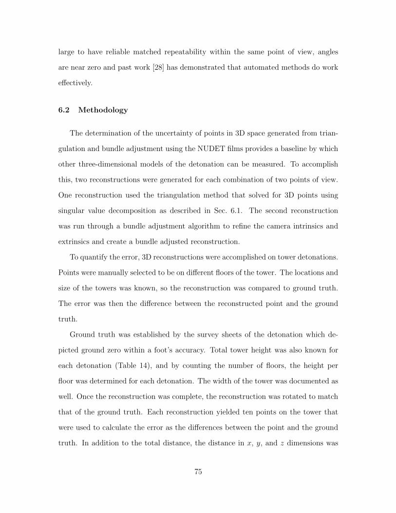
large to have reliable matched repeatability within the same point of view, angles

are near zero and past work [28] has demonstrated that automated methods do work

effectively.

6.2 Methodology

The determination of the uncertainty of points in 3D space generated from trian-

gulation and bundle adjustment using the NUDET films provides a baseline by which

other three-dimensional models of the detonation can be measured. To accomplish

this, two reconstructions were generated for each combination of two points of view.

One reconstruction used the triangulation method that solved for 3D points using

singular value decomposition as described in Sec. 6.1. The second reconstruction

was run through a bundle adjustment algorithm to refine the camera intrinsics and

extrinsics and create a bundle adjusted reconstruction.

To quantify the error, 3D reconstructions were accomplished on tower detonations.

Points were manually selected to be on different floors of the tower. The locations and

size of the towers was known, so the reconstruction was compared to ground truth.

The error was then the difference between the reconstructed point and the ground

truth.

Ground truth was established by the survey sheets of the detonation which de-

picted ground zero within a foot’s accuracy. Total tower height was also known for

each detonation (Table 14), and by counting the number of floors, the height per

floor was determined for each detonation. The width of the tower was documented as

well. Once the reconstruction was complete, the reconstruction was rotated to match

that of the ground truth. Each reconstruction yielded ten points on the tower that

were used to calculate the error as the differences between the point and the ground

truth. In addition to the total distance, the distance in x, y, and z dimensions was

75

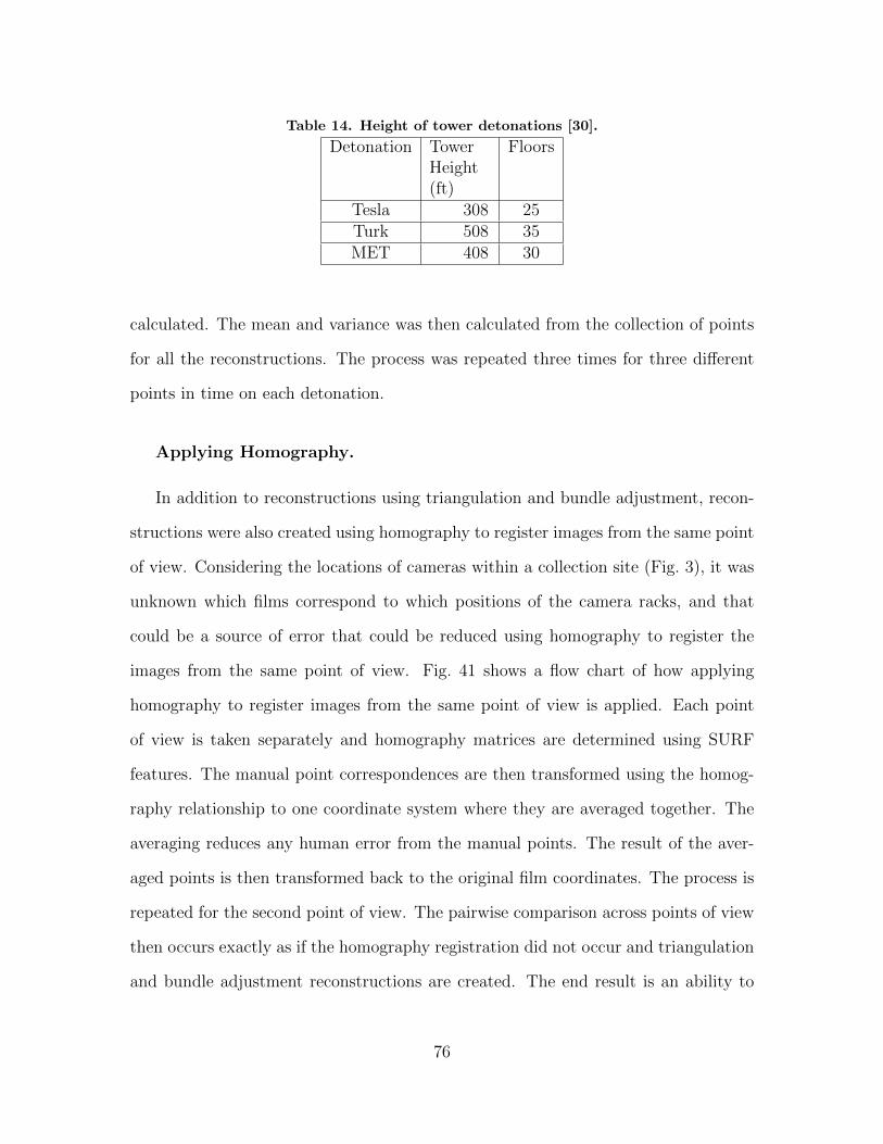
Table 14. Height of tower detonations [30].

Detonation TowerHeight(ft)

Floors

Tesla 308 25Turk 508 35MET 408 30

calculated. The mean and variance was then calculated from the collection of points

for all the reconstructions. The process was repeated three times for three different

points in time on each detonation.

Applying Homography.

In addition to reconstructions using triangulation and bundle adjustment, recon-

structions were also created using homography to register images from the same point

of view. Considering the locations of cameras within a collection site (Fig. 3), it was

unknown which films correspond to which positions of the camera racks, and that

could be a source of error that could be reduced using homography to register the

images from the same point of view. Fig. 41 shows a flow chart of how applying

homography to register images from the same point of view is applied. Each point

of view is taken separately and homography matrices are determined using SURF

features. The manual point correspondences are then transformed using the homog-

raphy relationship to one coordinate system where they are averaged together. The

averaging reduces any human error from the manual points. The result of the aver-

aged points is then transformed back to the original film coordinates. The process is

repeated for the second point of view. The pairwise comparison across points of view

then occurs exactly as if the homography registration did not occur and triangulation

and bundle adjustment reconstructions are created. The end result is an ability to

76

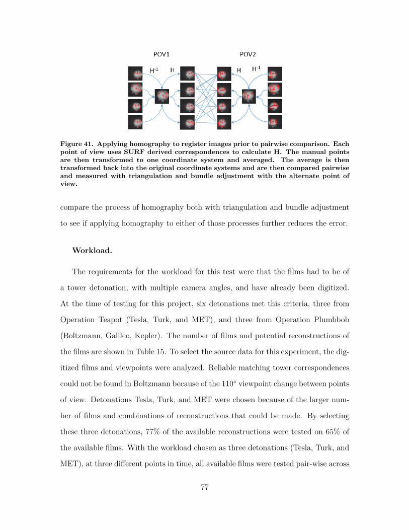
Figure 41. Applying homography to register images prior to pairwise comparison. Eachpoint of view uses SURF derived correspondences to calculate H. The manual pointsare then transformed to one coordinate system and averaged. The average is thentransformed back into the original coordinate systems and are then compared pairwiseand measured with triangulation and bundle adjustment with the alternate point ofview.

compare the process of homography both with triangulation and bundle adjustment

to see if applying homography to either of those processes further reduces the error.

Workload.

The requirements for the workload for this test were that the films had to be of

a tower detonation, with multiple camera angles, and have already been digitized.

At the time of testing for this project, six detonations met this criteria, three from

Operation Teapot (Tesla, Turk, and MET), and three from Operation Plumbbob

(Boltzmann, Galileo, Kepler). The number of films and potential reconstructions of

the films are shown in Table 15. To select the source data for this experiment, the dig-

itized films and viewpoints were analyzed. Reliable matching tower correspondences

could not be found in Boltzmann because of the 110◦ viewpoint change between points

of view. Detonations Tesla, Turk, and MET were chosen because of the larger num-

ber of films and combinations of reconstructions that could be made. By selecting

these three detonations, 77% of the available reconstructions were tested on 65% of

the available films. With the workload chosen as three detonations (Tesla, Turk, and

MET), at three different points in time, all available films were tested pair-wise across

77

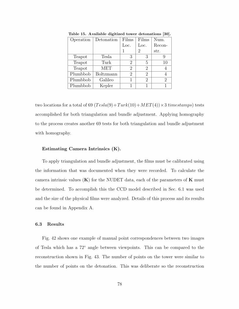
Table 15. Available digitized tower detonations [30].

Operation Detonation FilmsLoc.1

FilmsLoc.2

Num.Recon-str.

Teapot Tesla 3 3 9Teapot Turk 2 5 10Teapot MET 2 2 4

Plumbbob Boltzmann 2 2 4Plumbbob Galileo 1 2 2Plumbbob Kepler 1 1 1

two locations for a total of 69 (Tesla(9)+Turk(10)+MET (4))×3 timestamps) tests

accomplished for both triangulation and bundle adjustment. Applying homography

to the process creates another 69 tests for both triangulation and bundle adjustment

with homography.

Estimating Camera Intrinsics (K).

To apply triangulation and bundle adjustment, the films must be calibrated using

the information that was documented when they were recorded. To calculate the

camera intrinsic values (K) for the NUDET data, each of the parameters of K must

be determined. To accomplish this the CCD model described in Sec. 6.1 was used

and the size of the physical films were analyzed. Details of this process and its results

can be found in Appendix A.

6.3 Results

Fig. 42 shows one example of manual point correspondences between two images

of Tesla which has a 72◦ angle between viewpoints. This can be compared to the

reconstruction shown in Fig. 43. The number of points on the tower were similar to

the number of points on the detonation. This was deliberate so the reconstruction

78

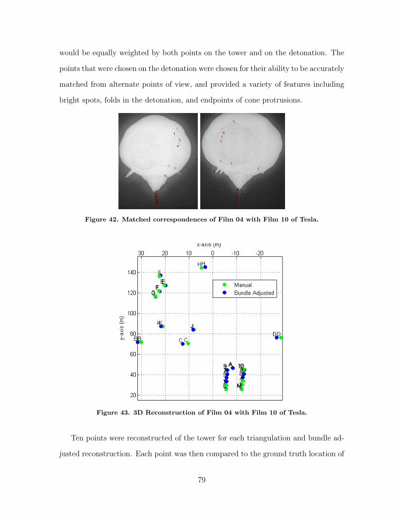
would be equally weighted by both points on the tower and on the detonation. The

points that were chosen on the detonation were chosen for their ability to be accurately

matched from alternate points of view, and provided a variety of features including

bright spots, folds in the detonation, and endpoints of cone protrusions.

Figure 42. Matched correspondences of Film 04 with Film 10 of Tesla.

Figure 43. 3D Reconstruction of Film 04 with Film 10 of Tesla.

Ten points were reconstructed of the tower for each triangulation and bundle ad-

justed reconstruction. Each point was then compared to the ground truth location of

79

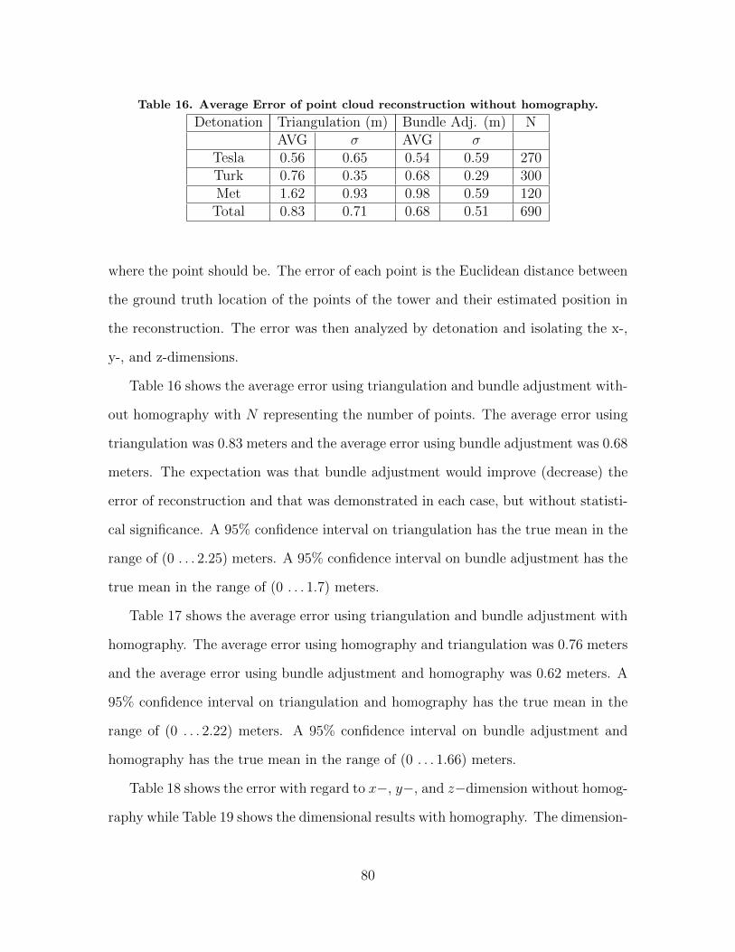
Table 16. Average Error of point cloud reconstruction without homography.

Detonation Triangulation (m) Bundle Adj. (m) NAVG σ AVG σ

Tesla 0.56 0.65 0.54 0.59 270Turk 0.76 0.35 0.68 0.29 300Met 1.62 0.93 0.98 0.59 120

Total 0.83 0.71 0.68 0.51 690

where the point should be. The error of each point is the Euclidean distance between

the ground truth location of the points of the tower and their estimated position in

the reconstruction. The error was then analyzed by detonation and isolating the x-,

y-, and z-dimensions.

Table 16 shows the average error using triangulation and bundle adjustment with-

out homography with N representing the number of points. The average error using

triangulation was 0.83 meters and the average error using bundle adjustment was 0.68

meters. The expectation was that bundle adjustment would improve (decrease) the

error of reconstruction and that was demonstrated in each case, but without statisti-

cal significance. A 95% confidence interval on triangulation has the true mean in the

range of (0 . . . 2.25) meters. A 95% confidence interval on bundle adjustment has the

true mean in the range of (0 . . . 1.7) meters.

Table 17 shows the average error using triangulation and bundle adjustment with

homography. The average error using homography and triangulation was 0.76 meters

and the average error using bundle adjustment and homography was 0.62 meters. A

95% confidence interval on triangulation and homography has the true mean in the

range of (0 . . . 2.22) meters. A 95% confidence interval on bundle adjustment and

homography has the true mean in the range of (0 . . . 1.66) meters.

Table 18 shows the error with regard to x−, y−, and z−dimension without homog-

raphy while Table 19 shows the dimensional results with homography. The dimension-

80

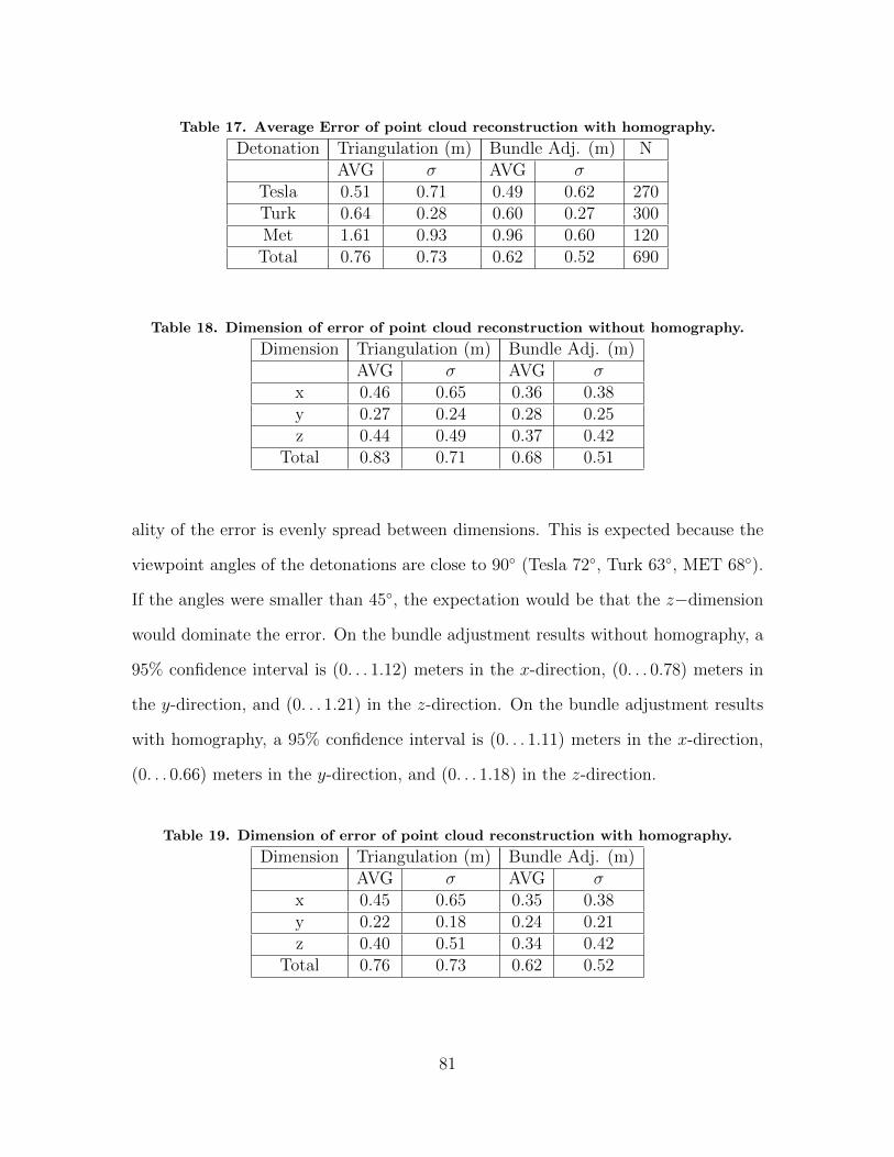
Table 17. Average Error of point cloud reconstruction with homography.

Detonation Triangulation (m) Bundle Adj. (m) NAVG σ AVG σ

Tesla 0.51 0.71 0.49 0.62 270Turk 0.64 0.28 0.60 0.27 300Met 1.61 0.93 0.96 0.60 120

Total 0.76 0.73 0.62 0.52 690

Table 18. Dimension of error of point cloud reconstruction without homography.

Dimension Triangulation (m) Bundle Adj. (m)AVG σ AVG σ

x 0.46 0.65 0.36 0.38y 0.27 0.24 0.28 0.25z 0.44 0.49 0.37 0.42

Total 0.83 0.71 0.68 0.51

ality of the error is evenly spread between dimensions. This is expected because the

viewpoint angles of the detonations are close to 90◦ (Tesla 72◦, Turk 63◦, MET 68◦).

If the angles were smaller than 45◦, the expectation would be that the z−dimension

would dominate the error. On the bundle adjustment results without homography, a

95% confidence interval is (0. . . 1.12) meters in the x-direction, (0. . . 0.78) meters in

the y-direction, and (0. . . 1.21) in the z-direction. On the bundle adjustment results

with homography, a 95% confidence interval is (0. . . 1.11) meters in the x-direction,

(0. . . 0.66) meters in the y-direction, and (0. . . 1.18) in the z-direction.

Table 19. Dimension of error of point cloud reconstruction with homography.

Dimension Triangulation (m) Bundle Adj. (m)AVG σ AVG σ

x 0.45 0.65 0.35 0.38y 0.22 0.18 0.24 0.21z 0.40 0.51 0.34 0.42

Total 0.76 0.73 0.62 0.52

81

Ground truth of the locations of points on the detonations are not known. To

estimate the locations of points on detonations the techniques of triangulation and

bundle adjustment were applied to points on a detonation and points on the detona-

tion’s tower where ground truth was known. Since the process of choosing points and

the technique applied in reconstruction are consistent for the reconstruction, the error

associated with the points with known ground truth can be inferred on the points

where ground truth is not known. The locational error of the points of the tower then

become the locational error of the points on the detonation.

6.4 Discussion

The results shown in Tables 18 and 19 provides the information necessary to

estimate the spacial accuracy of points in an atmospheric nuclear detonation. With

this new information, 3D point correspondences can be generated over a period or

region of interest in a detonation enabling the study of regional areas of a detonation

whose behavior is different than existing models. These point correspondences can

be used to test the accuracy of other models by comparing the models to the point

correspondence during that period in time.

One example of using this information for further research would be to track how

points on the detonation change over time (Chapter VII).The change of location of the

same points over time can be used to model how the detonation propagates in complex

areas of the detonation, where the detonation interacts with objects or changes in

atmospheric density. Using data assimilation [13] to fuse established mathematical

models with the nuclear images and how they change over time would be a logical

way to improve the accuracy of estimating the positional accuracy.

Another example would be to verify an estimate of volume generated from a

single image. An assumption could be made that since the edges of a detonation

82

appear spherical, then the entire detonation is spherical. The results of a bundle

adjusted reconstruction can generate points on the detonation recreating the depth

component of the detonation at those points. The points can then be compared

to a spherical rendering of the detonation to determine how accurate the spherical

assumption is. If the edges of the sphere are within the error of reconstruction,

the assumption would be confirmed as acceptable. Further assumptions could be

made that the detonation is not spherical, but rather an ellipsoid with symmetric

horizontal and depth components, but a differing vertical component. The differences

between 3D point reconstructions and sphere could be compared to that of a 3D point

reconstructions and an ellipsoid leading to conclusions that one model is more accurate

than another. These comparisons are not possible without the understanding of the

accuracy of the point correspondence grounded in truth locations that this process

establishes.

6.5 Conclusions

This chapter presents a method to quantify the positional error of points in a

3D point cloud generated from triangulation and bundle adjusted reconstructions of

nuclear material in a nuclear detonation. To quantify the positional error, 276 recon-

structions were accomplished on 50% of applicable digitized detonations to estimate

the positions of the support tower used in detonations. Ten points in each reconstruc-

tion were then compared to location information recorded at the time of detonation

to estimate the positional error of a point. Reconstruction via triangulation was com-

pared to reconstruction using bundle adjustment. Reconstructions using homography

were compared to reconstructions not using homography. Using homography to reg-

ister films from the same point of view and using bundle adjustment produces the

best results. The error of a given point using homography and bundle adjustment can

83

be estimated with an average positional error of 0.62 meters with 0.35, 0.24, and 0.34

meters of uncertainty in x-, y-, and z-directions respectively. The three dimensional

data sets created and the quantified error associated with 3D point reconstructions

provides a method to verify volume-based models of nuclear detonations.

84

VII. Estimating Atmospheric Nuclear Detonation Volume

With the ability to determine 3D point clouds on the surface of the detonation, and

the ability to detect subsphere features, the focus now turns to using that information

to estimate volume of a detonation over time. Four detonations were analyzed with

six volume generation methods: 1) sphere from 2D image, 2) ellipsoid from 2D image,

3) ellipsoid from 2D image augmented by subspheres, 4) sphere from 3D point cloud,

5) ellipsoid from 3D point cloud, and 6) space silhouette carving. Results show that

3D point cloud models are accurate in modeling detonation behavior in 3D space,

but 2D models have the lowest variability when applied to estimate nuclear yields.

Space carve models have low enough uncertainty to improve on radius-based models,

but suffer from over estimation if there are not enough viewpoints.

The remainder of this chapter is organized as follows. Sec. 7.1 discusses the

processes that were used to generate volume from the images and Sec. 7.2 discusses the

detonations that were analyzed. Sec. 7.3 presents the results and Sec. 7.4 concludes

the chapter.

7.1 Volume Estimation Processes

Six processes were used in estimating the volume of an explosion and the results

were compared. The first assumes that the explosion is spherical and the estimates

for the radius of the sphere are determined by a 2D image. The second assumes that

the explosion is a 3D ellipsoid. The third assumes that the big explosion is a 3D

ellipsoid with spherical subspheres protruding from it. The fourth volume estimation

process generates a sphere from a 3D point cloud of points on the surface of the

detonation. The fifth process generates an ellipsoid that is symmetric about the

depth and horizontal axis from the same 3D point cloud. The sixth and final process

85

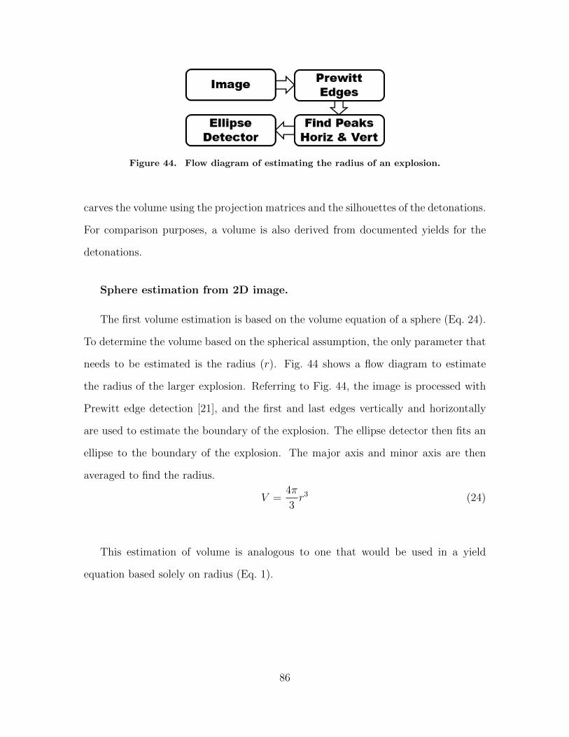
Figure 44. Flow diagram of estimating the radius of an explosion.

carves the volume using the projection matrices and the silhouettes of the detonations.

For comparison purposes, a volume is also derived from documented yields for the

detonations.

Sphere estimation from 2D image.

The first volume estimation is based on the volume equation of a sphere (Eq. 24).

To determine the volume based on the spherical assumption, the only parameter that

needs to be estimated is the radius (r). Fig. 44 shows a flow diagram to estimate

the radius of the larger explosion. Referring to Fig. 44, the image is processed with

Prewitt edge detection [21], and the first and last edges vertically and horizontally

are used to estimate the boundary of the explosion. The ellipse detector then fits an

ellipse to the boundary of the explosion. The major axis and minor axis are then

averaged to find the radius.

V =4π

3r3 (24)

This estimation of volume is analogous to one that would be used in a yield

equation based solely on radius (Eq. 1).

86

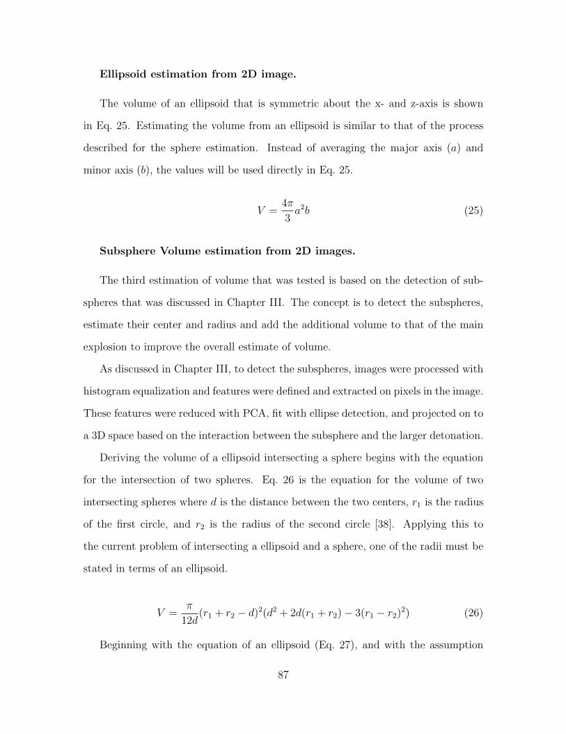
Ellipsoid estimation from 2D image.

The volume of an ellipsoid that is symmetric about the x- and z-axis is shown

in Eq. 25. Estimating the volume from an ellipsoid is similar to that of the process

described for the sphere estimation. Instead of averaging the major axis (a) and

minor axis (b), the values will be used directly in Eq. 25.

V =4π

3a2b (25)

Subsphere Volume estimation from 2D images.

The third estimation of volume that was tested is based on the detection of sub-

spheres that was discussed in Chapter III. The concept is to detect the subspheres,

estimate their center and radius and add the additional volume to that of the main

explosion to improve the overall estimate of volume.

As discussed in Chapter III, to detect the subspheres, images were processed with

histogram equalization and features were defined and extracted on pixels in the image.

These features were reduced with PCA, fit with ellipse detection, and projected on to

a 3D space based on the interaction between the subsphere and the larger detonation.

Deriving the volume of a ellipsoid intersecting a sphere begins with the equation

for the intersection of two spheres. Eq. 26 is the equation for the volume of two

intersecting spheres where d is the distance between the two centers, r1 is the radius

of the first circle, and r2 is the radius of the second circle [38]. Applying this to

the current problem of intersecting a ellipsoid and a sphere, one of the radii must be

stated in terms of an ellipsoid.

V =π

12d(r1 + r2 − d)2(d2 + 2d(r1 + r2)− 3(r1 − r2)2) (26)

Beginning with the equation of an ellipsoid (Eq. 27), and with the assumption

87

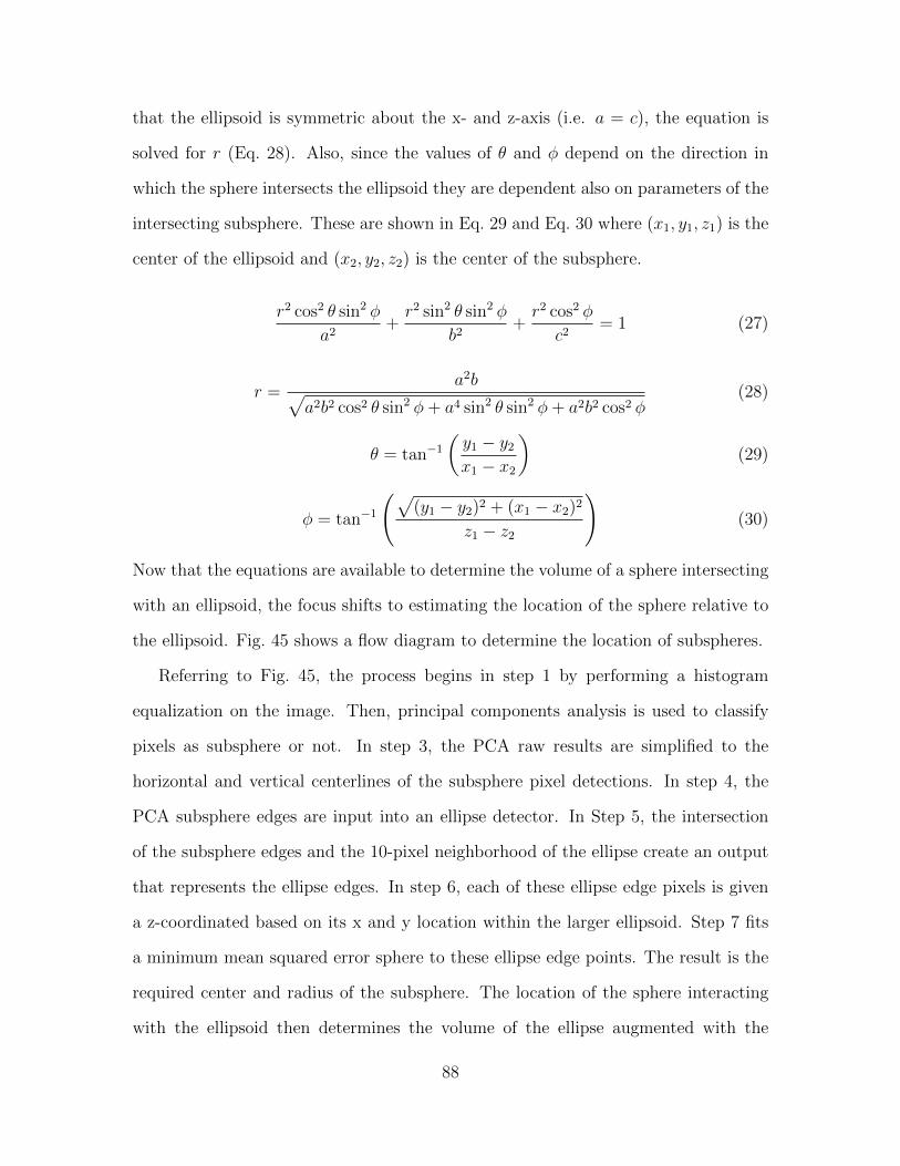
that the ellipsoid is symmetric about the x- and z-axis (i.e. a = c), the equation is

solved for r (Eq. 28). Also, since the values of θ and φ depend on the direction in

which the sphere intersects the ellipsoid they are dependent also on parameters of the

intersecting subsphere. These are shown in Eq. 29 and Eq. 30 where (x1, y1, z1) is the

center of the ellipsoid and (x2, y2, z2) is the center of the subsphere.

r2 cos2 θ sin2 φ

a2+r2 sin2 θ sin2 φ

b2+r2 cos2 φ

c2= 1 (27)

r =a2b√

a2b2 cos2 θ sin2 φ+ a4 sin2 θ sin2 φ+ a2b2 cos2 φ(28)

θ = tan−1

(y1 − y2

x1 − x2

)(29)

φ = tan−1

(√(y1 − y2)2 + (x1 − x2)2

z1 − z2

)(30)

Now that the equations are available to determine the volume of a sphere intersecting

with an ellipsoid, the focus shifts to estimating the location of the sphere relative to

the ellipsoid. Fig. 45 shows a flow diagram to determine the location of subspheres.

Referring to Fig. 45, the process begins in step 1 by performing a histogram

equalization on the image. Then, principal components analysis is used to classify

pixels as subsphere or not. In step 3, the PCA raw results are simplified to the

horizontal and vertical centerlines of the subsphere pixel detections. In step 4, the

PCA subsphere edges are input into an ellipse detector. In Step 5, the intersection

of the subsphere edges and the 10-pixel neighborhood of the ellipse create an output

that represents the ellipse edges. In step 6, each of these ellipse edge pixels is given

a z-coordinated based on its x and y location within the larger ellipsoid. Step 7 fits

a minimum mean squared error sphere to these ellipse edge points. The result is the

required center and radius of the subsphere. The location of the sphere interacting

with the ellipsoid then determines the volume of the ellipse augmented with the

88

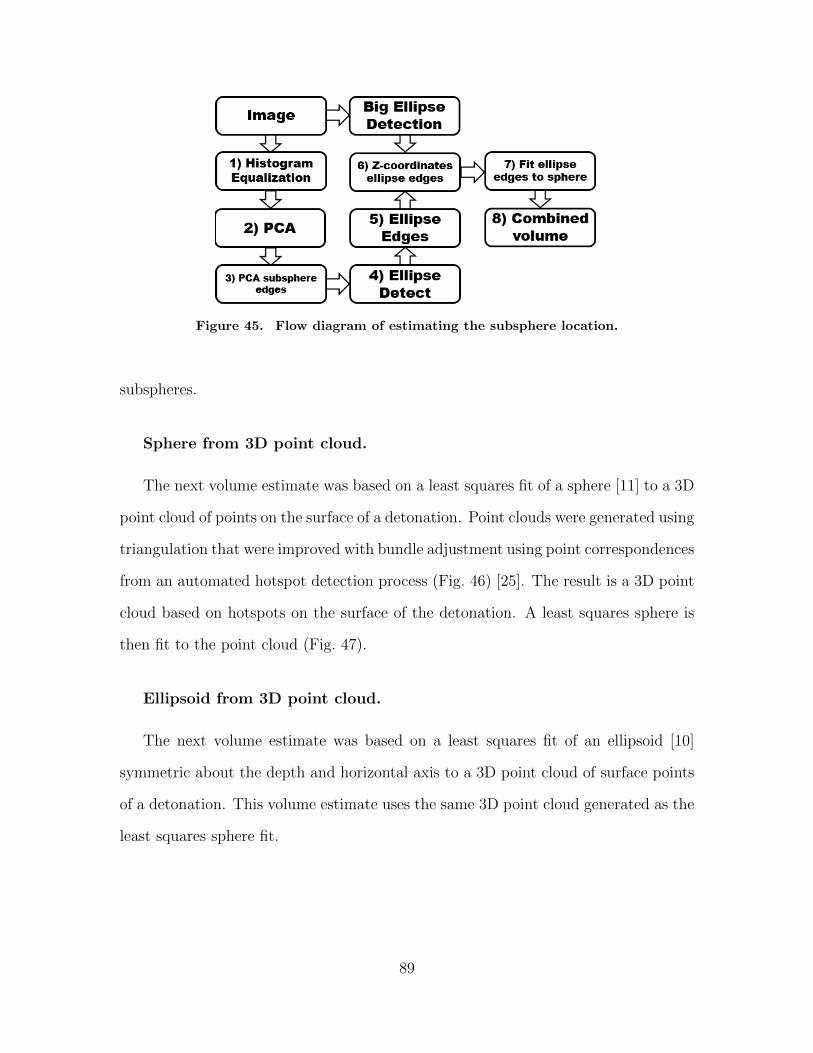
Figure 45. Flow diagram of estimating the subsphere location.

subspheres.

Sphere from 3D point cloud.

The next volume estimate was based on a least squares fit of a sphere [11] to a 3D

point cloud of points on the surface of a detonation. Point clouds were generated using

triangulation that were improved with bundle adjustment using point correspondences

from an automated hotspot detection process (Fig. 46) [25]. The result is a 3D point

cloud based on hotspots on the surface of the detonation. A least squares sphere is

then fit to the point cloud (Fig. 47).

Ellipsoid from 3D point cloud.

The next volume estimate was based on a least squares fit of an ellipsoid [10]

symmetric about the depth and horizontal axis to a 3D point cloud of surface points

of a detonation. This volume estimate uses the same 3D point cloud generated as the

least squares sphere fit.

89

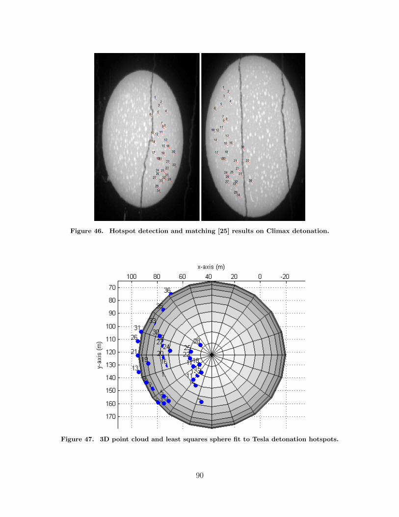
Figure 46. Hotspot detection and matching [25] results on Climax detonation.

Figure 47. 3D point cloud and least squares sphere fit to Tesla detonation hotspots.

90

Space Carving Volume.

The final volume estimate was based on space carving theory [12]. Images are

converted to silhouettes by detecting the edges of the detonation. Then, using the

refined projection matrices from bundle adjustment, the silhouettes are used to carve

out the volume of the detonation (Fig. 48).

Volume models using Homography.

Two additional volumes were generated using Homography (see Sec. 6.1) versions

of the 3D point clouds. The processes that were used in earlier testing (Sec. 6.2) that

saw reduction in errors and uncertainty were also used in volume estimation. This

results in models Sphere3D, and Ellipse3D with Homography.

Volume based on documented yields.

For comparison purposes, a volume was generated from the documented yields [6].

The equation used for this was the same as Taylor’s equation [36] in Eq. 2, just solved

for V resulting in

V = [Y ield× t2

po]35 .

The documented estimate of volumes are not ground truth, but are derived from

documented yields. For example, the documented yield [6] of Climax is 61 kT, but

recent research [30] has more accurately estimated it at 58.74 ± 0.19 kT. Even if the

documented values are not without error, they do provide a baseline for comparison.

91

Figure 48. Rendering of space carving results from two cameras of the MET detona-tion.

Table 20. Detonations tested.

Detonation Test Series Type Yield (kT)Climax [6] Upshot-Knothole Airdrop 58.74 [30]Grable [6] Upshot-Knothole Airdrop 15 [6]MET [6] Teapot Tower 22 [6]Tesla [6] Teapot Tower 7 [6]

7.2 Workload

Table 20 shows the detonations that were used for volume estimation. Two det-

onations (Climax and Grable) were chosen that were airdrops because they tend to

be more uniform in shape as a result of not having any obstructions to interfere with

the nuclear shock wave. An additional two detonations (MET and Tesla) were cho-

sen because they were tower detonations that demonstrated the subsphere features.

The ellipse plus subsphere approach was not attempted on the airdrop detonations

because of the lack of subspheres.

92

7.3 Results

The results of volume estimations for Climax, Grable, Tesla, and MET are shown

in Figs. 49, 50, 51, and 52 respectively. Table 21 shows the average residuals as

compared to the documented estimate of volume normalized using the average vol-

ume. Table 22 shows the standard deviation of the models resulting from a bisquare

weighted regression [3]. In all figures, it is apparent that the ellipsoid fit to a 3D point

cloud is the most unstable estimate as there are cases that are both significantly over

and under the documented estimate. Ellipsoid 3D volume instability is also evident

in Table 22 as the Ellipsoid 3D volume has the highest standard deviation (SD) of all

the volume estimates for every detonation. It is also clear that despite wide ranging

assumptions in the different volume methodologies, the estimates are all generally

consistent with each other and follow the same trend as the documented estimate.

The analysis here will focus on the SD of the results. The average difference be-

tween the documented estimate is less important because it is based on a documented

yield that may be incorrect. Overall, the 2D estimates have the least amount of vari-

ability. The volumes consistently climb as time increases, with the exception of small

drops caused by incorrect ellipse detections. The variance decreases slightly as the

method changes from 2D sphere to 2D ellipsoid to 2D ellipsoid + subsphere.

Considering the 3D volume estimates, the variance is higher than the 2D estimates.

For yield models to be improved by a volume-based model, the SD of the volume

models must be no more than three times the SD of the radius models. This can be

analyzed by comparing the 2D SDs to the 3D SDs. Considering the Grable estimate

with Sphere 2D volume SD of 20, 928m3 × 3 = 62, 784m3 this is still smaller than

the Sphere 3D and Ellipse 3D with Homography with SD of 158,320 and 214,140 m3

respectively. This means that the Sphere 3D and Ellipse 3D models have too large

an uncertainty to improve over 2D models for the purpose of yield estimation. The

93

space carve model, however has SD of 44,917 m3 which is less than three times the

SD of radius models. The space carve model SD also has less uncertainty than three

times the Sphere 2D models in the Climax and Tesla detonations, but not the MET

detonation.

It is also notable that the volume estimates from space carving tended to run

consistently high. The reason for this is because of the lack of viewpoints applied

to the space carving model. The space carve model is designed for objects that are

photographed on a turntable with about 24 viewpoints evenly spread out every 15◦.

The object is then carved from a cube depending on the viewpoints. In the estimates

for detonation volume, viewpoints were limited and only two viewpoints were used

leaving a considerable volume uncarved from the original cube. While the estimates

run consistently high, it is, however, within expectations as estimates are no more

than twice the expected volume. This expectation is established by comparing the

volume of a sphere inscribed inside a cube. A sphere with radius r has volume

43πr3 u 4r3 while a cube has volume (2r)3 = 8r3. The statistics in Table 21 show this

over estimation between 13.96% and 51.47% for the detonations analyzed. Applying

more viewpoints would further reduce this over estimation of volume.

The assertion that adding additional viewpoints would reduce the over-estimation

problem was tested with an available third point of view for the Grable detonation.

Adding a third point of view has challenges in aligning three films with frames that

have similar time stamps. The result is a reduction in the number of available data

points that meet the time match criteria. Fig. 50 shows the results of a space carve

with three points of view. Table 23 compares the results of two points of view and

three points of view for space carving and Sphere 2D volume models. Referring to

Table 23, the over-estimation of volume using space carving is reduced from over-

estimating by 32.45% to under-estimating by 1.7 % as compared to the documented

94

Table 21. Average Volume Bias, Normalized as percentage.

Vol. Method Climax Grable MET TeslaSphere 3D -5.65 -11.56 10.25 -17.47

Sphere 3D w/ H -5.95 -12.3 8.28 -17.47Ellipsoid 3D -3.49 -6.57 7.23 1.09

Ellipsoid 3D w/ H -3.26 -8.15 5.63 1.09Space Carve 39.7 32.45 51.47 13.97Sphere 2D -1.41 -5.19 3.04 12.07

Ellipsoid 2D -1.08 -4.8 3.53 12.86Subsphere 2D N/A N/A 3.69 12.92

Table 22. Standard deviations of Volume estimates in cubic meters.

Vol. Method Climax Grable MET TeslaSphere 3D 3,190,400 160,110 901,340 71,473

Sphere 3D w/ H 1,222,700 158,320 804,000 71,473Ellipsoid 3D 3,579,900 211,520 1,024,300 95,061

Ellipsoid 3D w/ H 2,673,800 214,140 1,012,300 95,061Space Carve 556,260 44,917 406,820 5,001Sphere 2D 196,840 20,928 46,810 5,172

Ellipsoid 2D 190,140 20,095 47,547 8,186Subsphere 2D N/A N/A 46,542 7,982

estimate of yield. The SD on the three points of view of the space carve is greater

than three times the Sphere 2D model which is a result of the fewer points caused by

timing restrictions on aligning three films together. This would be expected to fall

back in line with more data tested as was the case with the two points of view.

In summarizing the results, the volume estimates are consistent with each other.

This consistency validates the 3D point clouds that were used to generate the 3D

volume estimates. The 2D models are still the most reliable for predicting yield.

For the 3D Sphere and 3D Ellipse models to improve upon the 2D models for yield

estimation, the SD in estimates must be reduced. The space carving model has a small

enough SD to improve over 2D models, and its over estimation could be improved

with more viewpoints if sufficient time aligned frames exist.

95

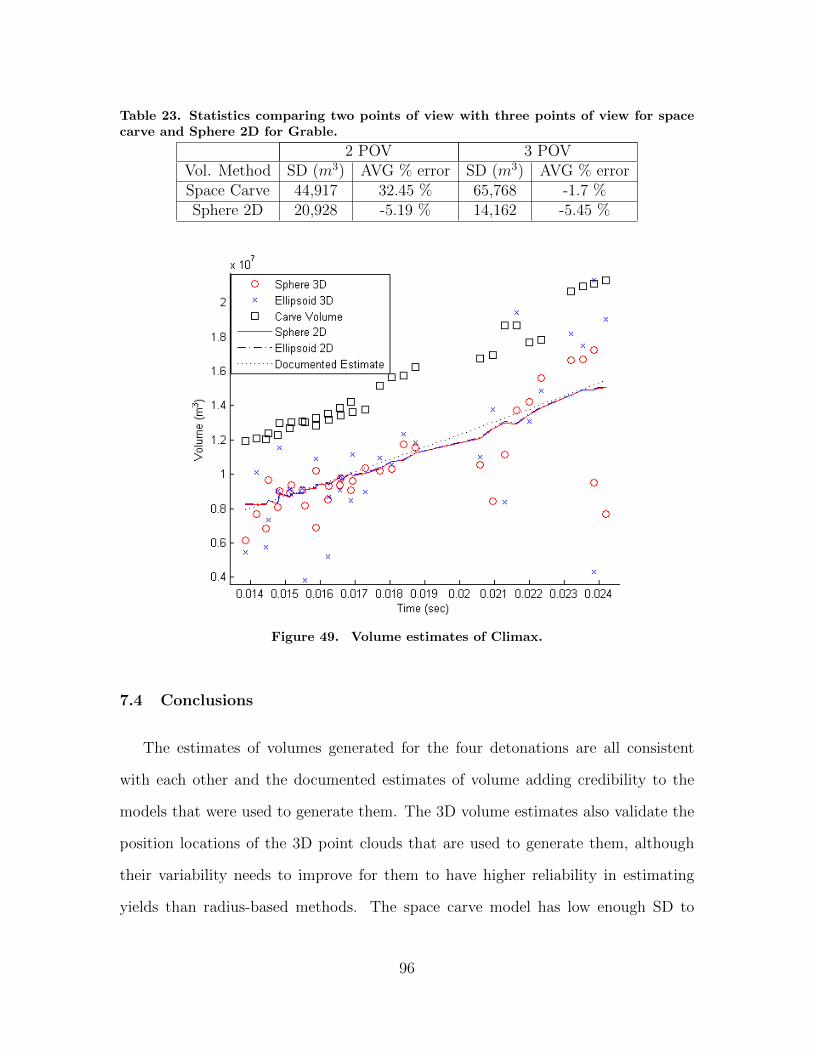
Table 23. Statistics comparing two points of view with three points of view for spacecarve and Sphere 2D for Grable.

2 POV 3 POVVol. Method SD (m3) AVG % error SD (m3) AVG % errorSpace Carve 44,917 32.45 % 65,768 -1.7 %Sphere 2D 20,928 -5.19 % 14,162 -5.45 %

Figure 49. Volume estimates of Climax.

7.4 Conclusions

The estimates of volumes generated for the four detonations are all consistent

with each other and the documented estimates of volume adding credibility to the

models that were used to generate them. The 3D volume estimates also validate the

position locations of the 3D point clouds that are used to generate them, although

their variability needs to improve for them to have higher reliability in estimating

yields than radius-based methods. The space carve model has low enough SD to

96

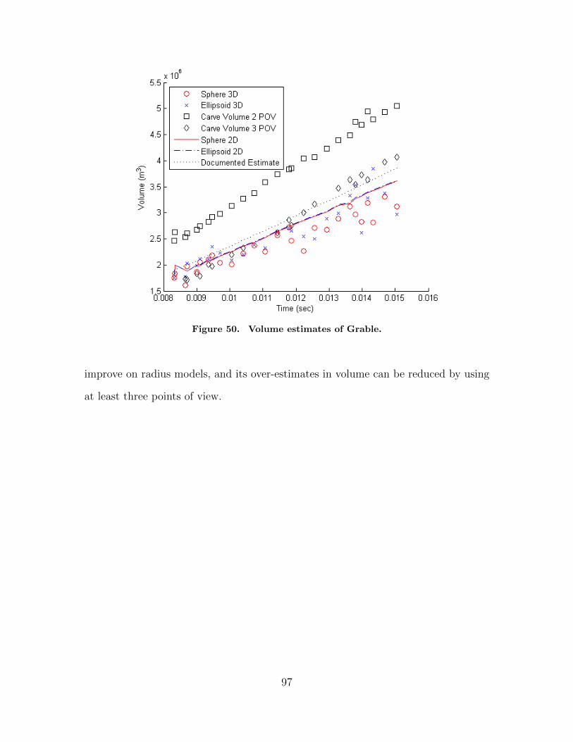
Figure 50. Volume estimates of Grable.

improve on radius models, and its over-estimates in volume can be reduced by using

at least three points of view.

97

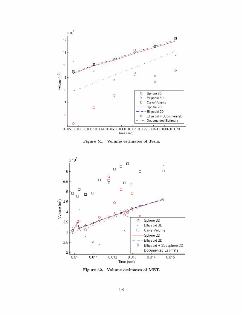
Figure 51. Volume estimates of Tesla.

Figure 52. Volume estimates of MET.

98

VIII. Conclusion and Future Work

The primary goal of this research was to provide an automated means to perform

three-dimensional analysis for atmospheric nuclear detonation films. It was hypothe-

sized that this could be accomplished by applying multi-view geometry and computer

vision techniques to the films in order to determine 3D positional information and

volume estimation over time. To accomplish this required alignment of the films in

time, detection of features in the images, matching of features, and multi-view re-

construction. Sub-explosion features were detected with 67% hit rate and 22% false

alarm rate. Hotspot features were detected with 71.95% hit rate, 86.03% precision

and a 0.015% false positive rate. Detected hotspots were matched across 57-109◦

viewpoints with 76.63% average correct matching by defining their location relative

to the center of the explosion, rotating them to the alternative viewpoint, and match-

ing them collectively. When 3D reconstruction was applied to the hotspot matching

it completed an automated process that was used to create 168 3D point clouds with

31.6 points per reconstruction with each point having an accuracy of 0.62 meters with

0.35, 0.24, and 0.34 meters of accuracy in the x-, y- and z-direction respectively. As

a demonstration of using the point clouds for analysis, volumes were estimated and

shown to be consistent with radius-based models and in some cases improve on the

level of uncertainty in the yield calculation.

8.1 Contributions

This document proposes the following contributions to the scientific community.

• The production of 3D sparse point clouds to track and study features of deto-

nations over time.

99

• An automated process to detect and match of hotspot features across wide

viewpoints.

In Chapter IV and V an automated hotspot feature detector and matching al-

gorithm was tested that matches hotspots across wide viewpoints using a spherical-

based object model. Hotspots can be detected with a 71.95% hit rate and 86.03%

precision. Hotspots are matched to films from wide viewpoints with 76.6% correct-

ness and a σ of 16.4% where the state-of-the-art matching techniques of SIFT and

SURF fail. Viewpoints were tested up to 109.5◦ significantly extending the viewpoint

matching capability. The addition of an automated techniques generated 168 3D re-

constructions across four detonations where manual reconstructions only were able to

generate nine 3D reconstructions during the same period of time. Within the NUDET

domain, the new automated technique provides the ability to study the NUDET in

three-dimensions. Outside the NUDET film domain, this demonstrates that a sphere

and polar coordinates can effectively be used to extend viewpoint matching when

objects in the image are spherical.

With regard to 3D positional estimation, the results of Chapter VI show that

using Homography and bundle adjustment that manually chosen points can be re-

constructed in three-dimensions with an average positional error of 0.62 meters with

0.35, 0.24, and 0.34 meters of uncertainty in x-, y-, and z-directions respectively. This

establishes a baseline of ground truth using the triangulation and bundle adjustment

techniques for the NUDET 3D point clouds. This improves the historical record of the

films by providing reliable, three-dimensional positional estimates of features within

a NUDET.

Lastly, volume estimations were derived from the films using six different volume

models. Yields estimated from these volumes were found to be consistent with radius-

based models. The space carve model did show low enough uncertainty to replace

100

radius-based models, but it needs at least three viewpoints to counteract the over-

estimation of volume.

8.2 Future Work

One item of future work would be to apply the automated hotspot matching

technique to more detonations. Other types of detonations like balloon suspended

detonations, surface detonations, and water surface detonations could be studied in

three-dimensions with greater accuracy and speed using the automated model. An

individual with expertise in physics could take the 3D point cloud results and interpret

them to see if it models can be defined that account for the changes in detonation

type from airdrop, balloon, tower and surface.

Another item of future work is to improve the techniques applied for volume

estimation to reduce the STD of volume estimations.

Another item that could be studied is another NUDET feature. This disserta-

tion showed that hotspots could be detected as well as subspheres, but cone features

or other features could be detected and fed into the automated viewpoint match-

ing model to match just like hotspots were. The hotspot feature detector could be

replaced with a more generic detector that doesn’t only consider hotspots, but all fea-

tures whether their light or dark contrasting with areas around it. This would likely

merge some capabilities of SIFT and SURF with the sphere-based wide-viewpoint

model making it more accessible outside the NUDET domain.

Another item that could be used to improve on the models presented would be

to correlate more than two views at a time. This dissertation focused on two points

of view because it was the most common case with availabe data that was of similar

distances which helped detection and matching of hotspots. But it is possible that

other data sets exist that either have a third site that is of similar distance to two

101

other sites, or could be correlated using features that are visible at varying distances.

With each additional viewpoints needing to be correlated in time with the others,

this is likely more difficult to find time aligned frames, but is quite possible.

Other future work could look into current day applications to build a system

using multiple cameras with atomic timing that could record non-nuclear detonations

and estimate their volumes using space carving. If such a system could accurately

estimate the volume of non-nuclear detonations, then it could provide the baseline

for a camera-only system for determining the yield of rogue devices.

Other work could test the feature detector and descriptor on other spherical based

objects to see how well it applies in the current day image domain of spherical objects

needing wide viewpoint matching capabilities.

Lastly, a study could characterize how accurate the current time models are by

using the 3D time sequenced hotspots with the inverse of the nuclear growth model to

determine time and compare it to the time estimated using the timing marks. There

are areas of certain films where the speed of the camera changes abruptly between

timing marks and this analysis would likely determine within a frame or two where

the anomaly occurs, instead of the current method that can only tell when the next

timing mark occurs (approx. 10-15 frames).

102

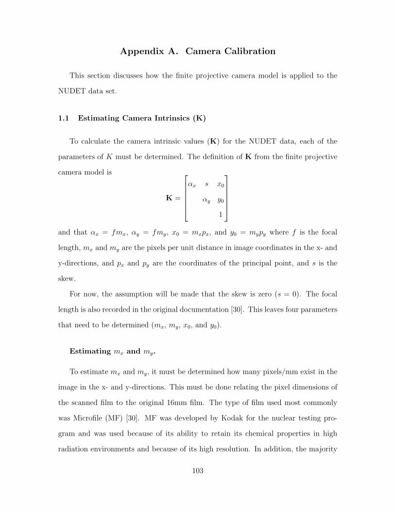
Appendix A. Camera Calibration

This section discusses how the finite projective camera model is applied to the

NUDET data set.

1.1 Estimating Camera Intrinsics (K)

To calculate the camera intrinsic values (K) for the NUDET data, each of the

parameters of K must be determined. The definition of K from the finite projective

camera model is

K =

αx s x0

αy y0

1

and that αx = fmx, αy = fmy, x0 = mxpx, and y0 = mypy where f is the focal

length, mx and my are the pixels per unit distance in image coordinates in the x- and

y-directions, and px and py are the coordinates of the principal point, and s is the

skew.

For now, the assumption will be made that the skew is zero (s = 0). The focal

length is also recorded in the original documentation [30]. This leaves four parameters

that need to be determined (mx, my, x0, and y0).

Estimating mx and my.

To estimate mx and my, it must be determined how many pixels/mm exist in the

image in the x- and y-directions. This must be done relating the pixel dimensions of

the scanned film to the original 16mm film. The type of film used most commonly

was Microfile (MF) [30]. MF was developed by Kodak for the nuclear testing pro-

gram and was used because of its ability to retain its chemical properties in high

radiation environments and because of its high resolution. In addition, the majority

103

of recordings were acrylate or polyethylene based black and white films which have an

expected lifespan of 100-500 years according to ANSI Standard IT9.11-1992. Fig. 53

shows the dimensions of the film that was used in filming [30]. All of the images

used were perforated two edges with Eastman Kodak long perforation (2R-3000).

The dimensions between perforations width-wise (distance F in Fig. 53) determines

the x dimensions. The dimensions between each perforation vertically (distance B

in Fig. 53) determines the y dimensions. Samples of each video were taken, and the

distance measured in the images in pixel length and related to the pixel lengths in the

x- and y-direction (10.49 mm and 7.62 mm respectively). As a result, an equation is

set for mx and my.

mx =horizontal pixel length between perforations

10.49mm

my =vertical pixel length between perforations

7.62mm

Measurements of at least 4 images were taken in the x- and y-direction and the

pixel difference was averaged for each film. To determine the vertical distance, subse-

quent frames were stacked vertically to recreate the continuous feel of the original film.

When this was accomplished it was determined that there was some overlap between

subsequent images of 10 pixels which could be visually determined by repetition in

the pixel pattern. After this 10 pixel overlap was removed from the y-distance the

results were accurately computed and are shown in Table 24.

Referring to Table 24, it is apparent that there was very little variation in the

measurement of x-distance. The maximum error was calculated based on the worse

case scenario that both the measurement error (σ) and the tolerance of the perforation

of the film were additive when in fact the error is likely that it is the larger of these

two errors. With this in consideration, all the variance in measurement is within

104

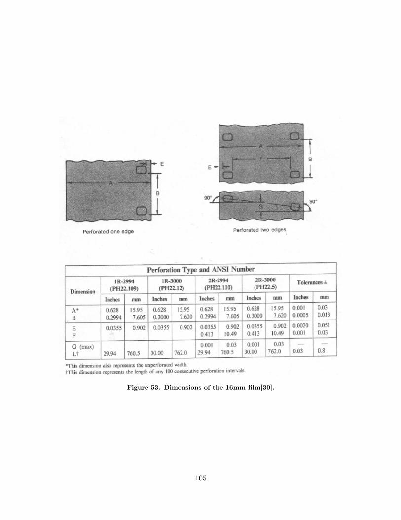
Figure 53. Dimensions of the 16mm film[30].

105

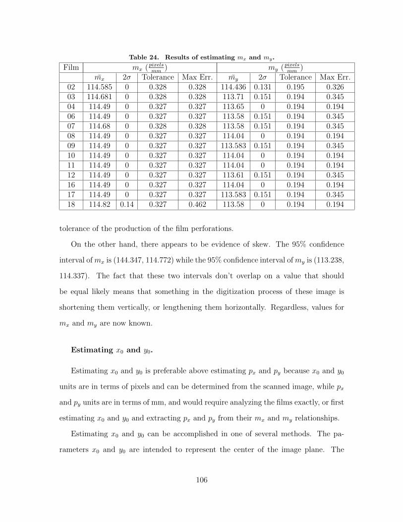
Table 24. Results of estimating mx and my.

Film mx (pixelsmm

) my (pixelsmm

)m̄x 2σ Tolerance Max Err. m̄y 2σ Tolerance Max Err.

02 114.585 0 0.328 0.328 114.436 0.131 0.195 0.32603 114.681 0 0.328 0.328 113.71 0.151 0.194 0.34504 114.49 0 0.327 0.327 113.65 0 0.194 0.19406 114.49 0 0.327 0.327 113.58 0.151 0.194 0.34507 114.68 0 0.328 0.328 113.58 0.151 0.194 0.34508 114.49 0 0.327 0.327 114.04 0 0.194 0.19409 114.49 0 0.327 0.327 113.583 0.151 0.194 0.34510 114.49 0 0.327 0.327 114.04 0 0.194 0.19411 114.49 0 0.327 0.327 114.04 0 0.194 0.19412 114.49 0 0.327 0.327 113.61 0.151 0.194 0.34516 114.49 0 0.327 0.327 114.04 0 0.194 0.19417 114.49 0 0.327 0.327 113.583 0.151 0.194 0.34518 114.82 0.14 0.327 0.462 113.58 0 0.194 0.194

tolerance of the production of the film perforations.

On the other hand, there appears to be evidence of skew. The 95% confidence

interval ofmx is (144.347, 114.772) while the 95% confidence interval ofmy is (113.238,

114.337). The fact that these two intervals don’t overlap on a value that should

be equal likely means that something in the digitization process of these image is

shortening them vertically, or lengthening them horizontally. Regardless, values for

mx and my are now known.

Estimating x0 and y0.

Estimating x0 and y0 is preferable above estimating px and py because x0 and y0

units are in terms of pixels and can be determined from the scanned image, while px

and py units are in terms of mm, and would require analyzing the films exactly, or first

estimating x0 and y0 and extracting px and py from their mx and my relationships.

Estimating x0 and y0 can be accomplished in one of several methods. The pa-

rameters x0 and y0 are intended to represent the center of the image plane. The

106

question then is, what is the image plane in this case? Three possible image planes

are considered with different definitions of the image plane. Also, Fig. 54 shows the

description of these different centers pictorially. Each of these are considered in turn.

1. Center of the resolution of the image

2. Center of the viewable portion of the image

3. Center of the emulsion layer of the image

Center of image. The center of the image is the most straight forward. It takes

the resolution of the image, and divides by 2 to get the center of the image. The

drawback is that some of the films are misaligned from left to right when they were

scanned.

Center of viewable area. The center of the viewable area on the image is also

straight forward. The film has borders on the left and right for the perforation of

the film. By removing the perforated areas, the actual area that contains images can

be isolated. This can remove any error that would result in misalignment of the film

when they were scanned.

Center of emulsion layer of film. Within the film itself there is a layer that is

intended to be exposed and collect the light particles. This layer is not always centered

with the film itself. It is ultimately the collector of photons. An argument could be

made that the emulsion layer represents the portion that was actually exposed to

light, and as a result the center of the of that area is truly the center of the image.

Prior to determining a center, a standard image crop was determined that removed

the left and right side perforated edges. To accomplish this, all the pixel values of all

the images of Tesla were summed column-wise. Then the local minimums on either

side of the plot was used as the cropping in the x-direction. This plot is shown in

Fig. 55. The end result is that cropping the image at 352, 1490 would be the best

107

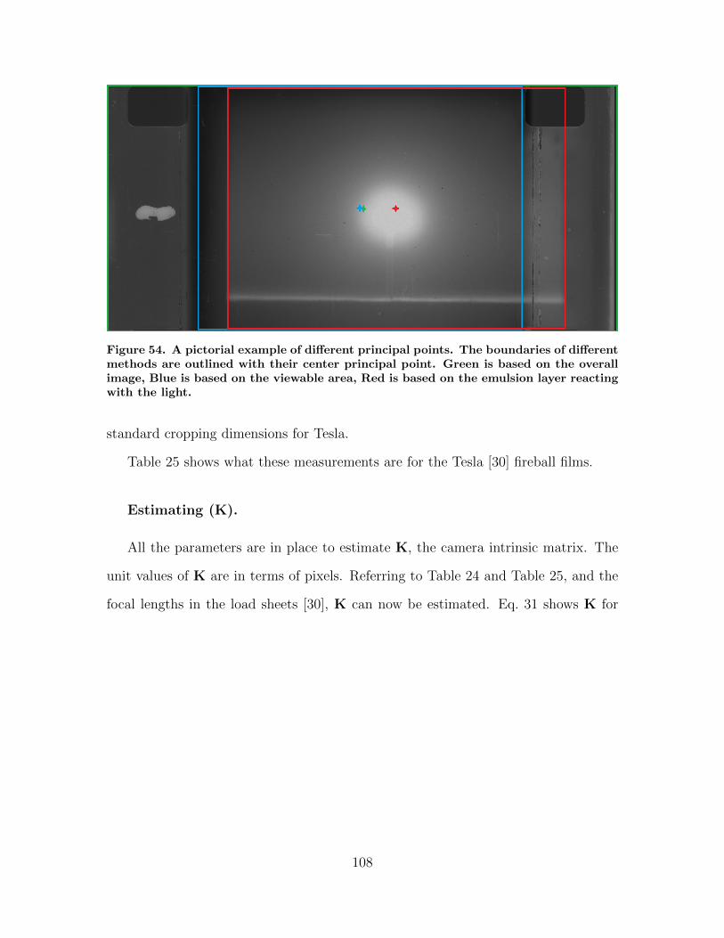
Figure 54. A pictorial example of different principal points. The boundaries of differentmethods are outlined with their center principal point. Green is based on the overallimage, Blue is based on the viewable area, Red is based on the emulsion layer reactingwith the light.

standard cropping dimensions for Tesla.

Table 25 shows what these measurements are for the Tesla [30] fireball films.

Estimating (K).

All the parameters are in place to estimate K, the camera intrinsic matrix. The

unit values of K are in terms of pixels. Referring to Table 24 and Table 25, and the

focal lengths in the load sheets [30], K can now be estimated. Eq. 31 shows K for

108

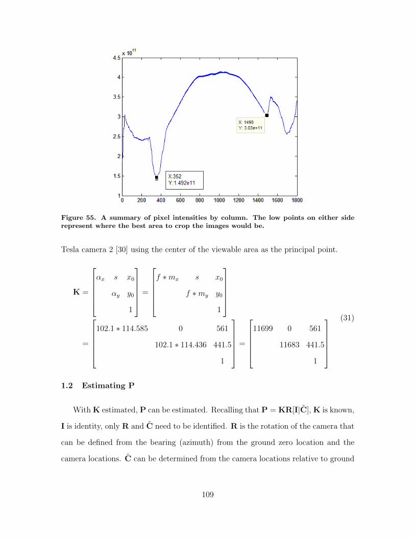
Figure 55. A summary of pixel intensities by column. The low points on either siderepresent where the best area to crop the images would be.

Tesla camera 2 [30] using the center of the viewable area as the principal point.

K =

αx s x0

αy y0

1

=

f ∗mx s x0

f ∗my y0

1

=

102.1 ∗ 114.585 0 561

102.1 ∗ 114.436 441.5

1

=

11699 0 561

11683 441.5

1

(31)

1.2 Estimating P

With K estimated, P can be estimated. Recalling that P = KR[I|C̃], K is known,

I is identity, only R and C̃ need to be identified. R is the rotation of the camera that

can be defined from the bearing (azimuth) from the ground zero location and the

camera locations. C̃ can be determined from the camera locations relative to ground

109

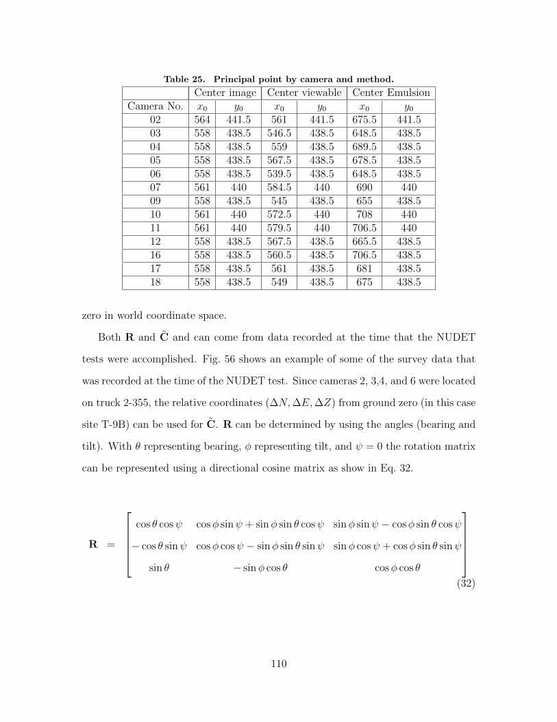
Table 25. Principal point by camera and method.

Center image Center viewable Center EmulsionCamera No. x0 y0 x0 y0 x0 y0

02 564 441.5 561 441.5 675.5 441.503 558 438.5 546.5 438.5 648.5 438.504 558 438.5 559 438.5 689.5 438.505 558 438.5 567.5 438.5 678.5 438.506 558 438.5 539.5 438.5 648.5 438.507 561 440 584.5 440 690 44009 558 438.5 545 438.5 655 438.510 561 440 572.5 440 708 44011 561 440 579.5 440 706.5 44012 558 438.5 567.5 438.5 665.5 438.516 558 438.5 560.5 438.5 706.5 438.517 558 438.5 561 438.5 681 438.518 558 438.5 549 438.5 675 438.5

zero in world coordinate space.

Both R and C̃ and can come from data recorded at the time that the NUDET

tests were accomplished. Fig. 56 shows an example of some of the survey data that

was recorded at the time of the NUDET test. Since cameras 2, 3,4, and 6 were located

on truck 2-355, the relative coordinates (∆N,∆E,∆Z) from ground zero (in this case

site T-9B) can be used for C̃. R can be determined by using the angles (bearing and

tilt). With θ representing bearing, φ representing tilt, and ψ = 0 the rotation matrix

can be represented using a directional cosine matrix as show in Eq. 32.

R =

cos θ cosψ cosφ sinψ + sinφ sin θ cosψ sinφ sinψ − cosφ sin θ cosψ

− cos θ sinψ cosφ cosψ − sinφ sin θ sinψ sinφ cosψ + cosφ sin θ sinψ

sin θ − sinφ cos θ cosφ cos θ

(32)

110

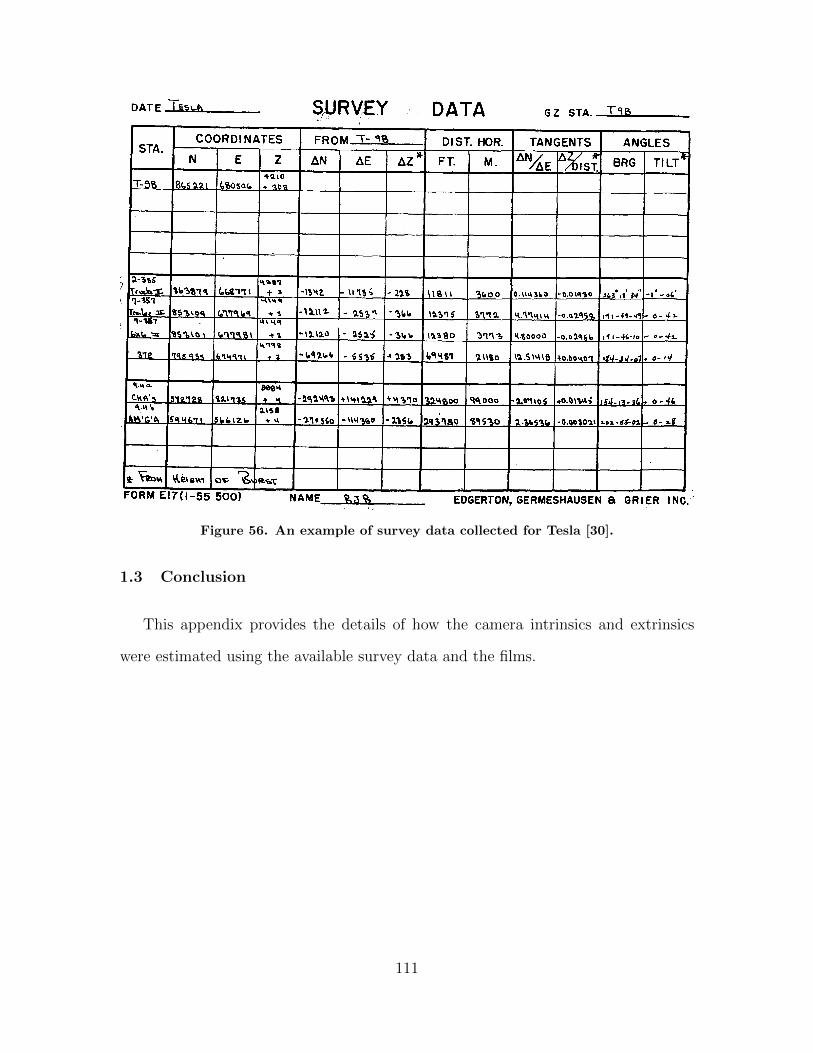
Figure 56. An example of survey data collected for Tesla [30].

1.3 Conclusion

This appendix provides the details of how the camera intrinsics and extrinsics

were estimated using the available survey data and the films.

111

Bibliography

1. Alpaydin, Ethem. Introduction to Machine Learning, 2nd edition. The MIT

Press, Cambridge, MA, 2010.

2. Bay, Herbert, Andreas Ess, Tinne Tuytelaars, and Luc Van Gool. “Speeded-Up

Robust Features (SURF)”. Computer Vision Image Understanding, 110(3):346–

359, June 2008. ISSN 1077-3142. URL http://dx.doi.org/10.1016/j.cviu.

2007.09.014.

3. Cleveland, William S. “Robust locally weighted regression and smoothing scat-

terplots”. Journal of the American Statistical Association, 74(368):829–836, 1979.

4. Duda, R.O. and P.E. Hart. Use of the Hough Transformation to Detect Lines

and Curves in Pictures. Technical Report 36, AI Center, SRI International, 333

Ravenswood Ave, Menlo Park, CA 94025, Apr 1971.

5. Fischler, Martin A. and Robert C. Bolles. “Random Sample Consensus: A

Paradigm for Model Fitting with Applications to Image Analysis and Automated

Cartography”. Communications of the ACM, 24(6):381–395, June 1981. ISSN

0001-0782. URL http://doi.acm.org/10.1145/358669.358692.

6. Gladeck, F. and A. Johnson. “For the Record - A History of the Nuclear Test

Personnel Review Program, 1978-1993”, March 1996.

7. Harris, Chris and Mike Stephens. “A combined corner and edge detector”. In

Proceedings of Fourth Alvey Vision Conference, 147–151. 1988.

8. Hartley, Richard and Andrew Zisserman. Multiple View Geometry in Computer

Vision. Cambridge University Press, New York, NY, USA, 2 edition, 2003. ISBN

0521540518.

112

9. Hartley, Richard I and Peter Sturm. “Triangulation”. Computer Vision and

Image Understanding, 68(2):146–157, 1997.

10. Hunyadi, Levente. “Fitting ellipses, ellipsoids and other

quadratic curves and surfaces”, 2014. Matlab File Exchange.

http://www.mathworks.com/matlabcentral/fileexchange/45356-fitting-

quadratic-curves-and-surfaces.

11. Jennings, Alan. “Sphere Fit (least squared)”. MATLAB Central. [Online.]

Available: http://www.mathworks.in/matlabcentral/fileexchange/34129-sphere-

fit–least-squared- .

12. Kutulakos, Kiriakos N. and Steven M. Seitz. “A Theory of Shape by Space

Carving”. International Journal Computer Vision, 38(3):199–218, July 2000.

ISSN 0920-5691. URL http://dx.doi.org/10.1023/A:1008191222954.

13. Le Dimet, F.-X., I. Souopgui, O. Titaud, V. Shutyaev, and M. Y. Hussaini. “To-

ward the assimilation of images”. Nonlinear Processes in Geophysics, 22(1):15–32,

2015. URL http://www.nonlin-processes-geophys.net/22/15/2015/.

14. Liu, H. and L. Yu. “Feature Selection for High-Dimensional Data: A Fast

Correlation-Based Filter Solution”. In Proceedings of The Twentieth Interna-

tional Conference on Machine Leaning (ICML-03), 856–863. ICM, Washington,

D.C., 2003.

15. Lowe, David G. “Distinctive Image Features from Scale-Invariant Keypoints”.

International Journal of Computer Vision, 60(2):91–110, January 2004.

16. Lynes, David. “An analysis of methods to determine nuclear weapon yield us-

ing digital fireball films”, Masters Thesis. March 2013. Air Force Institute of

Technology.

113

17. McKinney, Joseph. “Nuclear Test Films Timing Marks”, Oct 2013. Air Force

Institute of Technology. Presentation.

18. Morel, Jean-Michel and Guoshen Yu. “ASIFT: A new framework for fully affine

invariant image comparison”. SIAM Journal on Imaging Sciences, 2(2):438–469,

2009.

19. Oliensis, John. “The Least-Squares Error for Structure from Infinitesimal Mo-

tion.” International Journal of Computer Vision, 61(3):259–299, 2005. URL

http://dblp.uni-trier.de/db/journals/ijcv/ijcv61.html/Oliensis05.

20. Pacleb, Curtis W. “Analysis of the Nuclear Thermal Pulse using Digitized Scien-

tific Test Films”, Masters Thesis. March 2013. Air Force Institute of Technology.

21. Prewitt, J.M.S. “Object Enhancement and Extraction”. Picture Processing and

Psychopictorics, 75–149. Academic Press, 1970.

22. Reinsch, Christian H. “Smoothing by spline functions”. Numerische mathematik,

10(3):177–183, 1967.

23. Schmitt, Daniel T. and Gilbert L. Peterson. “Machine learning nuclear detonation

features”. Applied Imagery Pattern Recognition Workshop (AIPR), 2014 IEEE,

1–7. Oct 2014.

24. Schmitt, Daniel T. and Gilbert L. Peterson. “Timing mark detection on nuclear

detonation video”. Applied Imagery Pattern Recognition Workshop (AIPR), 2014

IEEE, 1–5. Oct 2014.

25. Schmitt, Daniel T. and Gilbert L. Peterson. “Feature Detection and Matching

on Atmospheric Nuclear Detonation Video”. IET Computer Vision Journal. Apr

2016. ‘To appear’.

114

26. Schmitt, Daniel T., Gibert L. Peterson, Robert Slaughter. “Quantifying 3D Po-

sitional Uncertainty of Radiological Material From Nuclear Detonation Video”.

Journal of Nuclear Science and Engineering, 181(2).

27. Seitz, Curless B. Diebel J. Scharstein D. Szeliski R., S. M. “A comparison and

evaluation of multi-view stereo reconstruction algorithms”. IEEE Computer So-

ciety Conference on Computer Vision and Pattern Recognition, 519–526, 2006.

28. Slaughter, Robert C., John W. McClory, Daniel T. Schmitt, Matthew D. Samb-

ora, and Karl C. Walli. “3D sparse point reconstructions of atmospheric nu-

clear detonations”. Applied Imagery Pattern Recognition Workshop (AIPR), 2014

IEEE, 1–9. Oct 2014.

29. Snavely, Noah, Steven M. Seitz, and Richard Szeliski. “Photo Tourism: Exploring

Photo Collections in 3D”. ACM Transactions on Graphics, 25(3):835–846, July

2006. ISSN 0730-0301. URL http://doi.acm.org/10.1145/1141911.1141964.

30. Spriggs, Gregory D. “Film Scanning Project”, Aug 2011. Lawrence Livermore

National Laboratory. Presentation.

31. Spriggs, Gregory D. “Nuclear Weapon Effects Laboratory Class”, Sept 2013.

Lawrence Livermore National Laboratory. Presentation.

32. Spriggs Gregory D., Ben Kowash, Kelianne Roberts. “Fireball Yield for Bee”,

Sept 2014. Lawrence Livermore National Laboratory. Presentation.

33. Sun, Yijun and Jian Li. “Iterative Relief for Feature Weighting”. Proceedings of

the 23rd International Conferene on Machine Learning, 913–920, 2006.

34. Szeliski, Richard. Computer Vision: Algorithms and Applications. Springer-

Verlag, London, 2011.

115

35. Szeliski, Richard and Sing Bing Kang. “Shape Ambiguities in Structure from

Motion”. IEEE Transactions on Pattern Analysis and Machine Intelligence,

19(5):506–512, May 1997. URL http://research.microsoft.com/apps/pubs/

default.aspx?id=75675.

36. Taylor, Geoffrey. “The Formation of a Blast Wave by a Very Intense Explo-

sion”. Proceedings of the Royal Society of London, volume 201, 159–174. Series

A, Mathematical and Physical Sciences, 1950.

37. Vedaldi, Andrea and Brian Fulkerson. “Vlfeat: An Open and Portable Library

of Computer Vision Algorithms”. Proceedings of the International Conference

on Multimedia, MM ’10, 1469–1472. ACM, New York, NY, USA, 2010. ISBN

978-1-60558-933-6. URL http://doi.acm.org/10.1145/1873951.1874249.

38. Weisstein, Eric W. “Sphere-Sphere Intersection”. From MathWorld–A Wolfram

Web Resource. http://mathworld.wolfram.com/Sphere-SphereIntersection.html.

39. Xie, Yonghong and Qiang Ji. “A New Efficient Ellipse Detection Method”. In-

ternation Conference on Pattern Recognition, 957–960. 2002.

40. Zeldovich, Y. B. Physics of Shock Waves and High-Temperature Hydrodynamic

Phenomena. Foreign Technology Division, 1965.

116

REPORT DOCUMENTATION PAGE Form Approved OMB No. 0704–0188

The public reporting burden for this collection of information is estimated to average 1 hour per response, including the time for reviewing instructions, searching existing data sources, gathering and maintaining the data needed, and completing and reviewing the collection of information. Send comments regarding this burden estimate or any other aspect of this collection of information, including suggestions for reducing this burden to Department of Defense, Washington Headquarters Services, Directorate for Information Operations and Reports (0704–0188), 1215 Jefferson Davis Highway, Suite 1204, Arlington, VA 22202–4302. Respondents should be aware that notwithstanding any other provision of law, no person shall be subject to any penalty for failing to comply with a collection of information if it does not display a currently valid OMB control number. PLEASE DO NOT RETURN YOUR FORM TO THE ABOVE ADDRESS. 1. REPORT DATE (DD–MM–YYYY) 24-03-2016

2. REPORT TYPE Dissertation

3. DATES COVERED (From — To) August 2013 – March 2016

4. TITLE AND SUBTITLE Position and Volume Estimation of Atmospheric Nuclear Detonations from Video Reconstruction

5a. CONTRACT NUMBER

5b. GRANT NUMBER

5c. PROGRAM ELEMENT NUMBER

6. AUTHOR(S) Schmitt, Daniel T., Lt Col, USAF

5d. PROJECT NUMBER 16P300 5e. TASK NUMBER

5f. WORK UNIT NUMBER

7. PERFORMING ORGANIZATION NAME(S) AND ADDRESS(ES) Air Force Institute of Technology Graduate School of Engineering and Management (AFIT/EN) 2950 Hobson Way WPAFB OH 45433-7765

8. PERFORMING ORGANIZATION REPORT NUMBER AFIT-ENG-DS-16-M-254

9. SPONSORING / MONITORING AGENCY NAME(S) AND ADDRESS(ES)

Defense Threat Reduction Agency ATTN: Maj Andrew Decker 8725 John J Kingman Rd Stop 6201 Fort Belvoir, VA 2206-6201 [email protected]

10. SPONSOR/MONITOR’S ACRONYM(S) DTRA

11. SPONSOR/MONITOR’S REPORT NUMBER(S)

12. DISTRIBUTION / AVAILABILITY STATEMENT DISTRIBUTION STATEMENT A: Approved for Public Release; Distribution Unlimited.

13. SUPPLEMENTARY NOTES This material is declared a work of the U.S. Government and is not subject to copyright protection in the United States

14. ABSTRACT Recent work in digitizing films of foundational atmospheric nuclear detonations from the 1950s provides an opportunity to perform deeper analysis on these historical tests. This work leverages multi-view geometry and computer vision techniques to provide an automated means to perform three-dimensional analysis of the blasts for several points in time. The accomplishment of this requires careful alignment of the films in time, detection of features in the images, matching of features, and multi-view reconstruction. Sub-explosion features can be detected with a 67% hit rate and 22% false alarm rate. Hotspot features can be detected with a 71.95% hit rate, 86.03% precision and a 0.015% false positive rate. Detected hotspots are matched across 57-109o viewpoints with 76.63% average correct matching by defining their location relative to the center of the explosion, rotating them to the alternative viewpoint, and matching them collectively. When 3D reconstruction is applied to the hotspot matching it completes an automated process that has been used to create 168 3D point clouds with 31.6 points per reconstruction with each point having an accuracy of 0.62 meters with 0.35, 0.24, and 0.34 meters of accuracy in the x-, y- and z-direction respectively. As a demonstration of using the point clouds for analysis, volumes are estimated and shown to be consistent with radius-based models and in some cases improve on the level of uncertainty in the yield calculation. 15. SUBJECT TERMS Multi-view Geometry, Nuclear Detonations, Nuclear Fireballs, Nuclear Effects, 3D Reconstruction, Feature Detection, Feature Matching, Computer Vision 16. SECURITY CLASSIFICATION OF: 17. LIMITATION

OF ABSTRACT UU

18. NUMBER OF PAGES 134

19a. NAME OF RESPONSIBLE PERSON Dr. Gilbert L. Peterson, AFIT/ENG

a. REPORT U

b. ABSTRACT U

c. THIS PAGE U

19b. TELEPHONE NUMBER (Include Area Code) (937) 255-3636 x 4281; [email protected]

Standard Form 298 (Rev. 8–98) Prescribed by ANSI Std. Z39.18

mailto:[email protected]

Documents

AIR FORCE INSTITUTE OF TECHNOLOGY - apps.dtic.mil · afit-eng-ds-16-m-254 position and volume estimation of atmospheric nuclear detonations from video reconstruction dissertation