Design of a Monocular Multi-Spectral Skin Detection,

Melanin Estimation, and False-Alarm Suppression System

THESIS

Keith R. Peskosky, Second Lieutenant, USAF

AFIT/GE/ENG/10-24

DEPARTMENT OF THE AIR FORCEAIR UNIVERSITY

AIR FORCE INSTITUTE OF TECHNOLOGY

Wright-Patterson Air Force Base, Ohio

APPROVED FOR PUBLIC RELEASE; DISTRIBUTION UNLIMITED.

The views expressed in this thesis are those of the author and do not reflect theofficial policy or position of the United States Air Force, Department of Defense, orthe United States Government.

AFIT/GE/ENG/10-24

Design of a Monocular Multi-Spectral Skin Detection,Melanin Estimation, and False-Alarm Suppression System

THESIS

Presented to the Faculty

Department of Electrical and Computer Engineering

Graduate School of Engineering and Management

Air Force Institute of Technology

Air University

Air Education and Training Command

In Partial Fulfillment of the Requirements for the

Degree of Master of Science in Electrical Engineering

Keith R. Peskosky, Bachelor of Science Electrical Engineering

Second Lieutenant, USAF

March 2010

APPROVED FOR PUBLIC RELEASE; DISTRIBUTION UNLIMITED.

AFIT/GE/ENG/10-24

Abstract

A real-time skin detection, false-alarm reduction, and melanin estimation system

is designed targeting search and rescue (SAR) with application to special operations

for manhunting and human measurement and signatures intelligence. A mathematical

model of the system is developed and used to determine how the physical system per-

forms under illumination, target-to-sensor distance, and target-type scenarios. This

aspect is important to the SAR community to gain an understanding of the deploya-

bility in different operating environments. A multi-spectral approach is developed and

consists of two short-wave infrared cameras and two visible cameras. Through an op-

tical chain of lenses, custom designed and fabricated dichroic mirrors, and filters, each

camera receives the correct spectral information to perform skin detection, melanin es-

timation, and false-alarm suppression. To get accurate skin detections under several

illumination conditions, the signal processing is accomplished in reflectance space,

which is estimated from known reflectance objects in the scene. Model-generated

output of imaged skin, when converted to estimated reflectance, indicates a good cor-

respondence with skin reflectance. Furthermore, measured and modeled estimates of

skin reflectance indicate a good correspondence with skin reflectance.

iv

Acknowledgements

Many thanks first of all go to my advisor. Without the countless hours of time spent

on helping me I would not been as successful as I was. To the EO crew thanks for all

the skiing, poker, bowling, and other random activities that were put together to get

out and do something new and exciting. Thanks also go to one of the only people I

know at AFIT that enjoys DCI as much as me. Thanks for being my wingman for

all the fine arts type events and for the great time beating up Nintendo characters.

Lastly, to my girlfriend, thank you so much for putting up with the many hours I

spent not being with you when you came out to visit me.

Keith R. Peskosky

v

Table of ContentsPage

Abstract . . . . . . . . . . . . . . . . . . . . . . . . . . . . . . . . . . . . . iv

Acknowledgements . . . . . . . . . . . . . . . . . . . . . . . . . . . . . . . v

List of Figures . . . . . . . . . . . . . . . . . . . . . . . . . . . . . . . . . viii

List of Tables . . . . . . . . . . . . . . . . . . . . . . . . . . . . . . . . . . xviii

I. Introduction . . . . . . . . . . . . . . . . . . . . . . . . . . . . . 1-11.1 Problem Statement . . . . . . . . . . . . . . . . . . . . . 1-21.2 Background and Related Research . . . . . . . . . . . . 1-5

1.3 Thesis Overview . . . . . . . . . . . . . . . . . . . . . . 1-8

II. Background . . . . . . . . . . . . . . . . . . . . . . . . . . . . . . 2-1

2.1 Reflectance Properties of Human Skin . . . . . . . . . . 2-1

2.2 Atmospheric Considerations . . . . . . . . . . . . . . . . 2-2

2.2.1 Solar Illumination . . . . . . . . . . . . . . . . . 2-42.2.2 Reflectance Estimation . . . . . . . . . . . . . . 2-6

2.3 Algorithms/Definitions . . . . . . . . . . . . . . . . . . . 2-7

2.3.1 Normalized Difference . . . . . . . . . . . . . . 2-72.3.2 Skin Detection . . . . . . . . . . . . . . . . . . 2-82.3.3 False-Alarm Reduction . . . . . . . . . . . . . . 2-92.3.4 Melanin Estimation . . . . . . . . . . . . . . . . 2-10

2.4 Geometric Optics . . . . . . . . . . . . . . . . . . . . . . 2-11

2.4.1 Fundamental Calculations . . . . . . . . . . . . 2-112.4.2 Diffraction and Aberrations . . . . . . . . . . . 2-13

2.5 Radiometry . . . . . . . . . . . . . . . . . . . . . . . . . 2-14

2.5.1 Solid Angle . . . . . . . . . . . . . . . . . . . . 2-14

2.5.2 Defining Radiometric Quantities . . . . . . . . . 2-16

2.5.3 Solving for Radiometric Quantities . . . . . . . 2-17

2.5.4 Modeling Illumination Sources . . . . . . . . . . 2-18

2.5.5 Atmospheric Attenuation . . . . . . . . . . . . . 2-19

2.5.6 Converting Photons to Electrons . . . . . . . . 2-20

2.6 Summary . . . . . . . . . . . . . . . . . . . . . . . . . . 2-21

vi

Page

III. Methodology . . . . . . . . . . . . . . . . . . . . . . . . . . . . . 3-1

3.1 Camera Selection . . . . . . . . . . . . . . . . . . . . . . 3-13.1.1 Near-Infrared Cameras . . . . . . . . . . . . . . 3-23.1.2 Visible Cameras . . . . . . . . . . . . . . . . . . 3-2

3.2 Lens Selection . . . . . . . . . . . . . . . . . . . . . . . . 3-73.2.1 Fore Optic (Front Lens) . . . . . . . . . . . . . 3-8

3.2.2 Color Camera Lens . . . . . . . . . . . . . . . . 3-113.2.3 Monochrome Camera Lens . . . . . . . . . . . . 3-13

3.3 Dichroic Mirrors . . . . . . . . . . . . . . . . . . . . . . 3-153.4 Filters . . . . . . . . . . . . . . . . . . . . . . . . . . . . 3-183.5 Radiometric Model . . . . . . . . . . . . . . . . . . . . . 3-20

3.5.1 Indoor Scenario Radiometry . . . . . . . . . . . 3-21

3.5.2 Modeling the Physical System . . . . . . . . . . 3-26

3.6 Summary . . . . . . . . . . . . . . . . . . . . . . . . . . 3-33

IV. Results and Analysis . . . . . . . . . . . . . . . . . . . . . . . . . 4-1

4.1 Qualitative Analysis . . . . . . . . . . . . . . . . . . . . 4-1

4.1.1 Visual Assessment of Image Quality . . . . . . . 4-1

4.1.2 Addressing Image Quality Issues for Camera 1and Camera 2 . . . . . . . . . . . . . . . . . . . 4-2

4.1.3 Addressing Image Quality Issues for Camera 3and Camera 4 . . . . . . . . . . . . . . . . . . . 4-4

4.2 Quantitative Analysis . . . . . . . . . . . . . . . . . . . 4-6

4.2.1 Comparing Estimated Reflectance From the Phys-ical System to Measured Reflectance . . . . . . 4-6

4.2.2 Comparing Modeled and Measured Reflectance 4-14

4.2.3 Comparing the Physical System and the Theoret-ical Model . . . . . . . . . . . . . . . . . . . . . 4-17

4.3 Operational Analysis . . . . . . . . . . . . . . . . . . . . 4-18

4.3.1 Basic Skin Detection . . . . . . . . . . . . . . . 4-184.3.2 False-Alarm Suppression . . . . . . . . . . . . . 4-18

4.3.3 Rule-Based Skin Detection . . . . . . . . . . . . 4-204.3.4 Melanin Estimation . . . . . . . . . . . . . . . . 4-20

4.4 Summary . . . . . . . . . . . . . . . . . . . . . . . . . . 4-22

V. Conclusion . . . . . . . . . . . . . . . . . . . . . . . . . . . . . . 5-15.1 Summary . . . . . . . . . . . . . . . . . . . . . . . . . . 5-1

5.2 Possibility of Future Work . . . . . . . . . . . . . . . . . 5-1

5.3 Concluding Remarks . . . . . . . . . . . . . . . . . . . . 5-2

Bibliography . . . . . . . . . . . . . . . . . . . . . . . . . . . . . . . . . . BIB-1

vii

List of FiguresFigure Page

1.1. To scale 2in pixels corresponding to the measured head and hand

size. This shows the best case scenario with pure skin pixels

shown in red. . . . . . . . . . . . . . . . . . . . . . . . . . . . . 1-3

1.2. To scale 2in pixels corresponding to the measured head and hand

size. This shows the worst case scenario with the pure skin pixels

shown in red. . . . . . . . . . . . . . . . . . . . . . . . . . . . . 1-4

1.3. Data acquisition scenario for search and rescue where the search

aircraft flies at approximately 500 ft above ground level and cam-

era system is aimed at an approximate 45 depression angle and

30 off angle. . . . . . . . . . . . . . . . . . . . . . . . . . . . . 1-5

1.4. Block diagram for the monocular skin detection, melanin esti-

mation, and false-alarm suppression camera system developed in

this thesis. . . . . . . . . . . . . . . . . . . . . . . . . . . . . . 1-6

1.5. (Top) RGB image of a test scene acquired with the HST3. (Bot-

tom) Skin detection performed on the above image, where the

image is colored based on melanin estimation [23]. . . . . . . . 1-7

1.6. Snapshot of the prototype two-band, real-time skin detection sys-

tem. . . . . . . . . . . . . . . . . . . . . . . . . . . . . . . . . . 1-8

1.7. (Top) Image seen through the 1080nm filter. (Middle) Image

seen through the 1550nm filter. (Bottom) Skin detection result-

ing from the skin detection methodology applied to the top and

middle images. . . . . . . . . . . . . . . . . . . . . . . . . . . . 1-9

1.8. Close in view of skin detection shown using the camera system

in Fig. 1.6. The false detections due to distance-dependent reg-

istration problems [23]. . . . . . . . . . . . . . . . . . . . . . . 1-10

viii

Figure Page

1.9. (Top) Transmission of the ThorLabs 1050nm center wavelength,

10nm bandwidth bandpass filter. (Note the filter’s measured

center wavelength is approximately 1053nm.) (Bottom) Trans-

mission of the ThorLabs 1550nm center wavelength, 12nm band-

width bandpass filter. Both band pass filters were measured by

a Casey spectrophotometer 5000. . . . . . . . . . . . . . . . . . 1-11

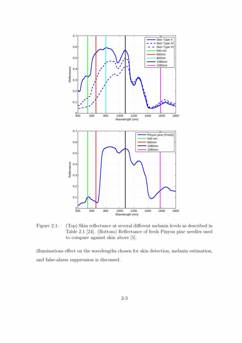
2.1. (Top) Skin reflectance at several different melanin levels as de-

scribed in Table 2.1 [24]. (Bottom) Reflectance of fresh Pinyon

pine needles used to compare against skin above [5]. . . . . . . 2-3

2.2. Water absorption coefficient as a function of wavelength [23]. . 2-4

2.3. Melanin absorption coefficient as a function of wavelength [23]. 2-4

2.4. This figure shows the measured oxygenated and deoxygenated

hemoglobin absorption of skin [23]. . . . . . . . . . . . . . . . . 2-5

2.5. (Solid) Solar irradiance in Dayton, OH on a sunny day scaled by

the maximum irradiance. (Dashed) The radiance spectra of Type

I/II skin illuminated by sunlight scaled by the same maximum

irradiance. The vertical lines show where 1080 and 1580nm are

located. . . . . . . . . . . . . . . . . . . . . . . . . . . . . . . . 2-5

2.6. Reflectance measurements of several items that have visible char-

acteristics of skin, but have dramatic differences in the NIR [23]. 2-8

2.7. Single lens imaging geometry. . . . . . . . . . . . . . . . . . . . 2-12

2.8. A multiple lens setup labeled with pertinent variables. . . . . . 2-13

2.9. Block diagram showing the necessary steps to model the system

from illumination to focal plane array. . . . . . . . . . . . . . . 2-15

2.10. (Left) Diagram showing pertinent variables required to solve for

the solid angle (Ω). (Right) Diagram used for demonstrating

differences when small angle assumption is used. . . . . . . . . 2-15

2.11. Diagram showing locations of θd and θs. . . . . . . . . . . . . . 2-17

ix

Figure Page

2.12. Three radiance blackbody curves with varying temperatures. The

sun is shown in the red curve with a temperature of 5950K. The

4500K temperature, in green, is an intermediate step to show

how the curves progress as the temperature changes. The ASD

Pro Lamps used in the study is represented with a 3200K black

body curve. . . . . . . . . . . . . . . . . . . . . . . . . . . . . . 2-19

2.13. Atmospheric extinction created in Laser Environmental Effects

Definition and Reference (LEEDR). This is used along with beer’s

law to estimate atmospheric transmission. . . . . . . . . . . . . 2-20

2.14. Two examples of using Beer’s law and how atmospheric transmis-

sion changes with respect to distance. (Left) Distance between

detector and source 2km. (Right) Distance between detector and

source 10km. . . . . . . . . . . . . . . . . . . . . . . . . . . . . 2-21

3.1. Block diagram for the monocular skin detection, melanin esti-

mation, and false-alarm suppression camera system developed in

this thesis. . . . . . . . . . . . . . . . . . . . . . . . . . . . . . 3-1

3.2. Relative response of the Goodrich SU640KTSX-1.7RT High Sen-

sitivity InGaAs short wave infrared camera. The absorption fea-

ture at 1380nm is due to atmospheric water absorption. Skin

detection bands are marked with vertical lines. . . . . . . . . . 3-3

3.3. Distance and direction a camera needs to move so that its pixel

size is the same as the Goodrich camera. The difference is calcu-

lated from a 150mm focus. Negative numbers refer to the camera

moving away from the lens while positive is moving towards. . 3-4

3.4. The depth of focus calculation with respect to f -number. . . . 3-5

3.5. Picture of the ThorLabs High Resolution USB2.0 CMOS Series

Cameras. . . . . . . . . . . . . . . . . . . . . . . . . . . . . . . 3-6

3.6. Relative Response of the ThorLabs DCC1645C. . . . . . . . . . 3-7

3.7. Relative Response of the ThorLabs DCC1545M. Even though

the plot shows an IR cut filter this camera model does not have

one. . . . . . . . . . . . . . . . . . . . . . . . . . . . . . . . . . 3-8

3.8. The image distance with respect to imaged pixel size for a 25µm

pixel calculated with the object distance set at 707ft. . . . . . . 3-9

x

Figure Page

3.9. System setup assuming the three dichroic mirrors are the same

size in order to approximate the minimum focal length that leaves

enough room for the mirrors. All blue arrows are 50mm in length. 3-10

3.10. To scale 1.41in pixels corresponding to the measured head and

hand size. This shows the best case scenario with the pure skin

pixels shown in red. . . . . . . . . . . . . . . . . . . . . . . . . 3-10

3.11. To scale 1.41in pixels corresponding to the measured head and

hand size. This shows the worst case scenario with the pure skin

pixels shown in red. . . . . . . . . . . . . . . . . . . . . . . . . 3-11

3.12. The imaged size of the 25µm pixels at different target distances.

These are calculated using a 150mm focal length lens. . . . . . 3-12

3.13. This figure demonstrates a safe distance between the fore optic

and correcting lenses so they will not hit the mirrors. . . . . . . 3-13

3.14. (Top) This plot shows what distances between lenses and focal

lengths are necessary to get the proper magnification of the pix-

els. (Bottom) Image Distance of two lens optical chain. (Red)

Object 31ft away from front lens. (Blue) Object 707ft away from

front lens. . . . . . . . . . . . . . . . . . . . . . . . . . . . . . . 3-14

3.15. Transmission of the ThorLabs LB1757 A coated lens measured

by ThorLabs using a spectrophotometer. . . . . . . . . . . . . . 3-15

3.16. (Top) This plot shows what distances between lenses and fo-

cal lengths are necessary to get the proper magnification of the

pixels. (Bottom) Image Distance of the two-lens optical chain.

(Red) Object 31ft away from front lens. (Blue) Object 707ft

away from front lens. . . . . . . . . . . . . . . . . . . . . . . . 3-16

3.17. Transmission of the ThorLabs LB1757 B coated lens measured

by ThorLabs using a spectrophotometer. . . . . . . . . . . . . . 3-17

3.18. Block diagram of the system with references for the path of the

light. . . . . . . . . . . . . . . . . . . . . . . . . . . . . . . . . 3-18

xi

Figure Page

3.19. Measured transmittance for Mirror 1. Green represents the rel-

evant reflected spectra and red represents the relevant transmis-

sion spectra for the skin detection, melanin estimation, and false-

alarm suppression tasks. The mirrors are measured in the same

45 orientation as they would be in the actual system. . . . . . 3-19

3.20. Measured transmittance for Mirror 2. Green represents the rel-

evant reflected spectra and red represents the relevant transmis-

sion spectra for the skin detection, melanin estimation, and false-

alarm suppression tasks. The mirrors are measured in the same

45 orientation as they would be in the actual system. . . . . . 3-20

3.21. Measured transmittance for Mirror 3. Green represents the rel-

evant reflected spectra and red represents the relevant transmis-

sion spectra for the skin detection, melanin estimation, and false-

alarm suppression tasks. The mirrors are measured in the same

45 orientation as they would be in the actual system. . . . . . 3-21

3.22. Measured transmission of the Semrock FF01-1060/13-25 NIR

bandpass filter at normal incidence. . . . . . . . . . . . . . . . 3-22

3.23. Measured transmission of the Semrock NIR01-1570/3-25 NIR

bandpass filter at normal incidence. . . . . . . . . . . . . . . . 3-23

3.24. Measured transmission of the Reynard Corporation R01718-00

long wave pass filter at normal incidence. . . . . . . . . . . . . 3-24

3.25. Top down view of the physical indoor setup for system testing

where, θd = 15 for each lamp and Rtargettolens = 31ft. Lamp

three’s θd is a depression angle. . . . . . . . . . . . . . . . . . . 3-24

3.26. Blackbody radiance curve for a single ASD pro lamp. . . . . . 3-25

3.27. The atmospheric transmission for a 20ft distance between the

lamps and target. . . . . . . . . . . . . . . . . . . . . . . . . . 3-25

3.28. The modeled irradiance on the target from three lamps. . . . . 3-26

3.29. The modeled exitance of the target for TypeI/II skin. . . . . . 3-27

3.30. The modeled radiance of the target for TypeI/II skin. . . . . . 3-27

xii

Figure Page

3.31. Spectral transmittance of all objects in the path of Camera 1

including the camera’s spectral response. The red, green, and

blue curves represent the amount of transmittance for each color

channel. . . . . . . . . . . . . . . . . . . . . . . . . . . . . . . . 3-29

3.32. (Left) Spectral transmittance of all objects in the path of Camera

2 not including the camera’s spectral response. (Right) Spectral

transmittance of all objects in the path of Camera 2 including

camera’s spectral response. The response is modeled at a value

of 1 until the cutoff wavelength of 1116nm where it is a value of

0. . . . . . . . . . . . . . . . . . . . . . . . . . . . . . . . . . . 3-30

3.33. (Left) Spectral transmittance of all objects in the path of Camera

3 not including the camera’s spectral response. (Right) Spectral

transmittance of all objects in the path of Camera 3 including

camera’s spectral response. The response is modeled at a value

of 0 until the cut on wavelength of 800nm where it is a value

of 1. The red curve shows the configuration without additional

filtering while the blue adds the Semrock bandpass filter. . . . 3-30

3.34. (Left) Spectral transmittance of all objects in the path of Camera

4 not including the camera’s spectral response. (Right) Spectral

transmittance of all objects in the path of Camera 4 including

camera’s spectral response. The response is modeled at a value

of 0 until the cut on wavelength of 800nm where it is a value

of 1. The red curve shows the configuration without additional

filtering, the green curve adds just the Semrock bandpass filter,

and the blue curves adds just the Reynard longwave pass filter. 3-31

3.35. Quantum efficiency of the ThorLabs silicon focal plane array. . 3-31

3.36. Quantum efficiency of the Goodrich InGaAs focal plane array. . 3-32

3.37. Reflectance of the white Labsphere Spectralonr panel. . . . . . 3-32

3.38. Reflectance of the gray Labsphere Spectralonr panel. . . . . . 3-33

4.1. Picture of the skin detection, melanin estimation, and false-alarm

suppression system designed and implemented in this thesis. . . 4-1

xiii

Figure Page

4.2. (Left) Image showing the highest visible quality image possi-

ble from Camera 1 by adjusting the focus and integration time.

(Right) Image showing the highest quality image possible from

Camera 3 by adjusting the focus and integration time. Note that

focus decreases from left to right in the image. . . . . . . . . . 4-2

4.3. (Left) Image acquired with the fore optic and ThorLabs DCC1645C

(Camera 1 ). Note the image quality in terms of focus improved

compared to Fig. 4.2. Issues with color seen are due to auto

coloring and gaining aspects from the manufacturer’s software.

(Right) Image acquired with the fore optic, second lens (Lens 1 ),

and the ThorLabs DCC1645C Camera 1, where decreased image

quality is seen. . . . . . . . . . . . . . . . . . . . . . . . . . . . 4-3

4.4. (Left) Image acquired with the fore optic, second lens (Lens 1 ),

iris diaphragm, and the ThorLabs DCC1645C (Camera 1 ). The

iris diaphragm is closed down to 8.3mm. (Right) Image acquired

with the fore optic, second lens (Lens 1 ), iris diaphragm, Mirror

1, and the ThorLabs DCC1645C (Camera 1 ). Some reduction in

image quality is seen due to the iris diaphragm not being centered

perfectly on the lens. . . . . . . . . . . . . . . . . . . . . . . . 4-4

4.5. (Left) Raw image from the ThorLabs DCC1645C used for ND-

GRI calculation (Camera 1 ). (Right) Raw image from the Thor-

Labs DCC1545M used for melanin estimation (Camera 2 ). . . 4-5

4.6. (Left) Raw image from the Goodrich SU640KTSX-1.7RT used

for skin detection (Camera 3 ) using the Semrock FF01-1060/13-

25 filter. This configuration results in the light transmitting to

(Camera 3 ) as shown in Fig 3.33 (blue curve). (Right) Raw

image from the Goodrich SU640KTSX-1.7RT used for skin de-

tection (Camera 4 ) using the Semrock NIR01-1570/3-25. This

configuration results in the light transmitting to the (Camera 4 )

as shown in Fig 3.34 (green curve). . . . . . . . . . . . . . . . . 4-5

xiv

Figure Page

4.7. (Left) Diffuse skin reflectance spectra obtained with a hand-held

reflectometer, of the test subject used in validating the opti-

cal system and model. (Right) The transmissions used in the

weighted average of the skin reflectance. The red and green

curves represent the RGB camera channel received spectra. The

cyan curve represents Camera 2’s, black represents Camera 3’s,

and maroon represents Camera 4’s transmission . . . . . . . . 4-7

4.8. (Left) Distribution of 2184 neck pixels for the green channel of

Camera 1. (Right) Distribution of 2184 neck pixels for the red

channel of Camera 1. The red line shows where the expected

diffuse skin reflectance is located, per Table 4.2. . . . . . . . . . 4-7

4.9. Estimated reflectance from Camera 2 using the raw data shown

in Fig. 4.5 (Right). . . . . . . . . . . . . . . . . . . . . . . . . . 4-8

4.10. Distribution of 1960 neck pixels for Camera 2. The red line

shows where the expected diffuse skin reflectance is located, per

Table 4.2. . . . . . . . . . . . . . . . . . . . . . . . . . . . . . . 4-9

4.11. (Left) Estimated reflectance from Camera 3 using the raw data

shown in Fig. 4.6. (Left) Estimated reflectance from Camera 4

using the raw data shown in Fig. 4.6 (Right). . . . . . . . . . . 4-9

4.12. (Left) Distribution of 2184 neck pixels for Camera 3. (Right)

Distribution of 2184 neck pixels for Camera 4. The red line

shows where the expected diffuse skin reflectance is located, per

Table 4.2. . . . . . . . . . . . . . . . . . . . . . . . . . . . . . . 4-10

4.13. (Top) Image acquired by HST3 used for comparison against the

skin detection system data. (Bottom) Masked version of the

image showing only Type I/II skin used in the analysis. . . . . 4-10

4.14. (Left) Distribution of the Type I/II skin pixels for the green

channel of the HST3 image. (Right) Distribution of the Type

I/II skin pixels for the red channel of the HST3 image. The red

line shows where the expected diffuse skin reflectance is located,

per Table 4.2. . . . . . . . . . . . . . . . . . . . . . . . . . . . 4-12

4.15. (Left) Distribution of the Type I/II skin pixels for the melanin

estimation channel of the HST3 image. The red line shows where

the expected diffuse skin reflectance is located, per Table 4.2. . 4-12

xv

Figure Page

4.16. (Left) Distribution of the Type I/II skin pixels for the filtered

1060nm channel of the HST3 image. (Right) Distribution of

the Type I/II skin pixels for the filtered 1570nm channel of the

HST3 image. The red line shows where the expected diffuse skin

reflectance is located, per Table 4.2. . . . . . . . . . . . . . . . 4-13

4.17. The Bhattacharyya coefficient comparing each of the designed

skin detection system distributions to the HST3 distributions.

Red and green correspond to the color channels for Camera 1 ;

Mel corresponds to Camera 2 ; 1060F and 1570F correspond to

the use of the Semrock bandpass filters on Camera 3 and Camera

4. . . . . . . . . . . . . . . . . . . . . . . . . . . . . . . . . . . 4-13

4.18. (Left) The number of electron-forming photons hitting the focal

plane array of each camera with three different targets. The red

× represents the white Spectralonr panel, green ∗ represents

skin, and blue represents the gray Spectralonr panel. The

labels on the x axis of red and green correspond the color chan-

nels for Camera 1 ; Mel corresponds to Camera 2 ; 1060NF and

1570NF correspond to what Camera 3 and Camera 4 see with

only their respective mirrors reflecting and transmitting; 1060F

and 1570F correspond to the use of the Semrock bandpass filters

on Camera 3 and Camera 4. Lastly, LWPF corresponds to the

use of the Reynard corporation longwave pass filter on Camera

4. (Right) The measured reflectance of each target shown in the

model. Red corresponds to the white panel, green corresponds

to skin, and blue corresponds to the gray panel reflectance. . . 4-15

4.19. The estimated reflectance of skin found by using empirical line

method represented as a red . Actual skin reflectance is repre-

sented by a blue ×. The labels on the x axis of red and green

correspond the color channels for Camera 1 ; Mel corresponds to

Camera 2 ; 1060NF and 1570NF correspond to what Camera 3

and Camera 4 see with only their respective mirrors reflecting

and transmitting; 1060F and 1570F correspond to the use of the

Semrock bandpass filters on Camera 3 and Camera 4. Lastly,

LWPF corresponds to the use of the Reynard corporation long-

wave pass filter on Camera 4. . . . . . . . . . . . . . . . . . . 4-16

xvi

Figure Page

4.20. The difference between the estimated and actual reflectance of

measured skin shown in Fig. 4.19. A negative value means the

estimated reflectance is higher than the actual reflectance. Red

and green labels correspond the color channels for Camera 1 ;

Mel corresponds to Camera 2 ; 1060NF and 1570NF correspond

to Camera 3 and Camera 4 see with only their respective mirrors

reflecting and transmitting; 1060F and 1570F correspond to the

use of the Semrock bandpass filters on Camera 3 and Camera 4.

Lastly, LWPF corresponds to the use of the Reynard corporation

longwave pass filter on Camera 4. . . . . . . . . . . . . . . . . 4-17

4.21. Comparison of the model and physical system results. The red

× represents the physical system’s estimated reflectance, green

∗ represents the model’s estimated reflectance, and blue repre-

sents the actual reflectance. Red and green correspond the color

channels for Camera 1 ; Mel corresponds to Camera 2 ; 1060F

and 1570F correspond to the use of the Semrock bandpass filters

on Camera 3 and Camera 4. . . . . . . . . . . . . . . . . . . . 4-19

4.22. (Left) NDSI calculated from the estimated reflectance of Camera

3 and 4. (Right) Skin detection using NDSI only accomplished

by setting bounded threshold between 0.5 and 0.95. . . . . . . 4-19

4.23. (Left) NDGRI calculated from the estimated reflectance of the

red and green channels of Camera 1. (Right) Pixels in the image

meeting the bounded threshold between -0.1 and -0.4. . . . . . 4-20

4.24. (Top) Image of the final detection after the bounded NDSI and

NDGRI detections are multiplied together. (Bottom) Color Im-

age of scene to compare skin detection against. . . . . . . . . . 4-21

xvii

List of TablesTable Page

1.1. Model shape and size of hand and head used in determining

required pixel sizes. Values are determined by measuring the

hand and head of a typical adult male. . . . . . . . . . . . . . . 1-3

2.1. Fitzpatrick scale used for describing skin color and sensitivity to

ultra violet light. These correspond to the skin types shown in

Fig. 2.1. . . . . . . . . . . . . . . . . . . . . . . . . . . . . . . . 2-2

2.2. Percentage of epidermis volume occupied by melanosomes with

respect to skin color. . . . . . . . . . . . . . . . . . . . . . . . . 2-2

2.3. The differences between the reflectance values of skin and plant

with respect to Fig. 2.1. . . . . . . . . . . . . . . . . . . . . . . 2-10

2.4. Radiometric Quantities . . . . . . . . . . . . . . . . . . . . . . 2-17

3.1. Specifications for the Goodrich SU640KTSX-1.7RT. . . . . . . 3-2

3.2. Pixel sizes used to calculate how far camera must be moved to

get same imaged size as 25µm. . . . . . . . . . . . . . . . . . . 3-4

3.3. Important specifications of the ThorLabs DCC1645C. . . . . . 3-6

3.4. Important specifications of the ThorLabs DCC1545M. . . . . . 3-7

3.5. Specifications of the PAC075 Newport Achromatic Double lens. 3-11

3.6. Specifications of the ThorLabs LB1757-A Lens. . . . . . . . . . 3-15

3.7. Specifications of the ThorLabs LB1757-B Lens. . . . . . . . . . 3-17

3.8. Wavelength transmission and reflection bands for mirrors 1, 2,

and 3 shown in Fig. 3.1. CW is the center wavelength of the

band . . . . . . . . . . . . . . . . . . . . . . . . . . . . . . . . . 3-19

3.9. The optical component order (OCO) for each camera’s optical

path including filter options. The attenuation of the incident

light is calculated with these objects in mind. (R) represents

reflection off mirror while (T) represents transmitting through. 3-29

xviii

Table Page

3.10. Table showing the reflectance values that should be estimated.

These values are based on the measured skin reflectance weighted

by the system transmission for each camera’s optical chain. . . 3-34

4.1. Camera settings used to acquire the images shown in Fig. 4.5

(Left,Right) and 4.6 (Left, Right). . . . . . . . . . . . . . . . . 4-4

4.2. Expected skin reflectance values generated by applying the trans-

mission curves of Fig. 4.7 (Right) to the skin reflectance in Fig. 4.7

(Left) used in comparing the model and the optical system. . . 4-6

xix

Design of a Monocular Multi-Spectral Skin Detection,

Melanin Estimation, and False-Alarm Suppression System

I. Introduction

Hyper and multi-spectral imaging is used in a wide range of scientific disciplines.

Recently, there has been a push towards the use of hyper-spectral imaging for search

and rescue missions. An example of this is the Civil Air Patrol’s Airborne Real-Time

Cueing Hyperspectral Enhanced Reconnaissance (ARCHER), which uses hyperspec-

tral data from 500-1100nm to help in Search and Rescue (SAR) missions [27]. For

use in the SAR application, hyper-spectral imagery requires high spatial and spec-

tral resolution. To meet these requirements, line scanning imagers must have a small

field of view (FOV) and scan quickly. The HyperSpecTIR 3 (HST3) line scanning

hyper-spectral camera used by the Sensors Exploitation Research Group takes about

10 seconds to scan an image, which is typical of line scanning instruments. The

slow acquisition makes the capture of motion, or use for real-time detection, infeasi-

ble. Following the work by Nunez [23], a real-time multi-spectral detection system is

developed.

The system developed in this thesis exploits the reflectance of human skin in the

near-infrared (NIR) to help identify it as a unique material of interest. The concept

has been proven to work with a hyper-spectral imager, and is mature enough to

be transformed into a compact monocular multi-spectral detection system. The skin

detection, false-alarm suppression, and melanin estimation system under development

uses the visible spectrum and three other specific wavelength bands, divided over four

cameras. Bands around 1080 and 1580nm are used for skin detection, while bands

around 800 and 1080nm are used for melanin estimation. The visible spectrum is

used for false-alarm suppression as well as a high-resolution color image of the scene.

A single fore optic is used to minimize registration problems, making the pixel-by-

1-1

pixel comparison faster and more accurate than a system with four separate objective

lenses.

A multi-spectral detection system of the type developed here has several poten-

tial uses. Search and Rescue is a demanding task that requires large teams of people

doing what is frequently a blind search. These searches can take more time than the

victim has to wait. Airborne searches rely on the talent, and in some cases luck, of

analysts and the imagery on hand. Although this does not seem to be a complete so-

lution, it should be able to take most of the guesswork out of the analysts’ job. This is

accomplished by providing a cueing mechanism, so the analysts can focus their image

collection and analysis efforts on the areas identified as having skin. Furthermore,

ground crews can be more efficiently tasked to those areas of interest. This system

further has an advantage over thermal detection, since it can detect the skin of living

or dead subjects. Special/covert operations may find this system useful, as the wave-

lengths used for skin detection and melanin estimation are beyond the visible light

spectrum. With near-infrared illumination, skin detection can be accomplished in low

light conditions, or even in the dark. Melanin estimation can make the searches for

missing people, or finding criminals on the run, much easier. The system designed

will moreover be used by other researchers to find ways to use specific human motion

and emotion to classify actions that could be a concern.

1.1 Problem Statement

A multi-spectral skin detection, melanin estimation, and false-alarm reduction

system is needed for the SAR problem. It must be able to image at a resolution of

no more than 2-inch pixels from a slant range of ∼710 feet. Based on the following

argument, 2×2 inch pixels were chosen to ensure that a few “pure skin pixels” of skin

are imaged. A rough measurement of a typical adult hand and head were made and

the results are shown in Table 1.1. The imaging scenario assumes that the camera,

hand, and head are aligned such that their major axis is aligned with the vertical

direction of the camera. The squares in Figures 1.1 and 1.2 represent the two inch

1-2

Table 1.1: Model shape and size of hand and head used in determining requiredpixel sizes. Values are determined by measuring the hand and head of atypical adult male.Body Part Modeled Shape Modeled Size (in)

Head Ellipse 8× 6Neck Rectangle 3.5× 5

Hand minus fingertips Rectangle 6× 3.5Fingertips Rectangle 1× 1.75

Figure 1.1: To scale 2in pixels corresponding to the measured head and hand size.This shows the best case scenario with pure skin pixels shown in red.

imaged pixels and are to scale with the modeled head and hand. The “pure skin

pixels” are colored in red so they can be easily seen. The best case scenario (Fig. 1.1),

using 2 × 2 inch pixels has 8 pixels on the head and 3 on the hand. The worst case

scenario (Fig. 1.2) gives 3 on the head and 0 on the hand. Even in the worst case

scenario, there are at least 2 “pure skin pixels” of skin for the system to detect.

This imaging distance is based on the assumption that the search aircraft flies at

500ft above ground level with a camera looking out at 45 and off to the side at 30, as

1-3

Figure 1.2: To scale 2in pixels corresponding to the measured head and hand size.This shows the worst case scenario with the pure skin pixels shown inred.

shown in Fig. 1.31. This system needs to acquire imagery and process it at a baseline

1fps. The cameras chosen are capable of higher frame rates, so as the detection

algorithms become faster, higher frame rates will be physically available. A single

fore optic is used to reduce registration problems inherent in multi-lens systems. The

system is additionally designed to remain a passive detection system, even in low-light

conditions. A model of this system is made to fine tune the detection thresholds.

To accomplish the stated requirements, six essential pieces must be considered:

fore optic, secondary lens (to account for the pixel size differences), iris diaphragms,

dichroic mirrors to efficiently segment the light energy, filters to focus on necessary

features, and cameras to perform the imaging. A block diagram of the system is

shown in Fig. 1.4.

1Private communications with Mr. Chris Rowley, President and Director of Operations, VolunteerImaging Analysts for Search and Rescue, March 2009,(http://www.viasar.org) [25]

1-4

Figure 1.3: Data acquisition scenario for search and rescue where the search aircraftflies at approximately 500 ft above ground level and camera system isaimed at an approximate 45 depression angle and 30 off angle.

1.2 Background and Related Research

The work in human skin detection that formed the basis for this thesis was

accomplished at the Air Force Institute of Technology in [23]. The author in [23]

created a diffuse model of human skin by examining its optical properties. From

this model, several scenarios were studied and efficient algorithms for skin detection,

false-alarm suppression, and melanin estimation were specified. The first attempt at

performing skin detection with sensors was with the HyperSpecTIR 3 (HST3). This is

1-5

Figure 1.4: Block diagram for the monocular skin detection, melanin estimation,and false-alarm suppression camera system developed in this thesis.

a hyperspectral imager designed by SpecTIR [16], originally for airborne applications.

The HST3 is a line scanning imager that uses scanning mirrors and a prism to divide

light into several hundred bands. The HST3 collects data in the range of 400-2500nm.

The spectral bands are sampled nominally at 11nm in the VIS and 8nm in the NIR.

The full width half maximum (FWHM) of each of the bands is approximately 14nm

and 8nm in the visible and NIR respectively.

Due to their often large nature and typical slow scan times, line scanning instru-

ments such as the HST3 are not necessarily the best option for use on small aircraft or

doing real-time detection. As stated above, it was the right type of imager for doing

preliminary work and demonstrating the potential on real images. An example of the

general capability of skin detection, false-alarm suppression, and melanin estimation

is shown in Fig. 1.5 where the are images taken with the HST3.

Since general wavelength bands were found from the theoretical modeling work

in conjunction with images from the HST3, a solution could be found that would

allow one to achieve real-time detection in the NIR. The initial concept work used a

stereo optic system using two Goodrich SUI640KTSX-1.7RT high sensitivity InGaAs

1-6

Figure 1.5: (Top) RGB image of a test scene acquired with the HST3. (Bottom)Skin detection performed on the above image, where the image is col-ored based on melanin estimation [23].

NIR cameras, each with their own lens and filter, as shown in Fig. 1.6. (The cameras

are discussed in more detail in Section 3.1.) Figure 1.7 shows an image from each

camera and the resulting skin detection. The false detections seen are due to low

power in the images or shadows.

The stereo optic approach has an inherent registration problem due to having

separate lenses. If such a system is fielded, it would require four cameras, each

with its own set of optics, which complicates the registration problem caused by

different objects at different distances in the scene. Figure 1.8 shows a close-up

picture of the stereo optic system performing skin detection, where the “target” is

holding the detection system display. The skin detection performs well but there are

false detections mostly at edges from objects occurring at different distances from

the camera. Another factor is the cost of buying four sets of optics, one for each

1-7

Figure 1.6: Snapshot of the prototype two-band, real-time skin detection system.

camera. The single optic design proposed in Fig. 1.4, removes the need for continuous

registration and several fore optic lenses.

The filters used on the two camera system were measured by a Casey spectropho-

tometer 5000 to determine their transmission properties. These filters are ThorLabs

25.4mm bandpass filters, which are specified as having center wavelengths of 1050 and

1550 and bandwidths of 10nm and 12nm respectively. Figure 1.9 shows the trans-

mission measured for each. Using these filters, the stereo optic system is receives at

most 60% of the incident light to the focal plane array. Furthermore, we see that the

1050nm center wavelengths is off by 3nm. A carefully designed optical system will

improve on the relatively poor performance exhibited by the prototype system.

1.3 Thesis Overview

Chapter II provides an introduction to radiometry and how it is used to de-

termine the spectral energy incident on the fore optic of the system and how many

electron forming photons will strike the focal plane array. The basics of skin de-

tection, false-alarm reduction, and melanin estimation are discussed. This includes

justification of specific wavelengths chosen as well as the algorithms used to perform

the detection. Additionally, specifics of the features subsequently used in detection,

false-alarm suppression, and melanin estimation are covered. Finally an overview of

1-8

Figure 1.7: (Top) Image seen through the 1080nm filter. (Middle) Image seenthrough the 1550nm filter. (Bottom) Skin detection resulting from theskin detection methodology applied to the top and middle images.

geometric optics is covered. Chapter III introduces the criteria from which the sys-

tem components are chosen, as well as the development of an optical model for the

1-9

Figure 1.8: Close in view of skin detection shown using the camera system inFig. 1.6. The false detections due to distance-dependent registrationproblems [23].

detection system. Chapter IV gives a comparison of the model results to real images

acquired with the developed system. Finally, Chapter V provides a summary of what

is done, the results, future work, and the contribution this thesis work has on SAR

and H-MASINT work.

1-10

1000 1010 1020 1030 1040 1050 1060 1070 1080 1090 11000

5

10

15

20

25

30

35

40

45

50T

rans

mis

sion

(%)

Wavelength (nm)

1500 1510 1520 1530 1540 1550 1560 1570 1580 1590 16000

10

20

30

40

50

60

Tra

nsm

issi

on(%

)

Wavelength (nm)

Figure 1.9: (Top) Transmission of the ThorLabs 1050nm center wavelength, 10nmbandwidth bandpass filter. (Note the filter’s measured center wave-length is approximately 1053nm.) (Bottom) Transmission of the Thor-Labs 1550nm center wavelength, 12nm bandwidth bandpass filter. Bothband pass filters were measured by a Casey spectrophotometer 5000.

1-11

II. Background

This chapter covers the background necessary to understand the features exploited

and methods used for skin detection which are necessary to build the system. The

reflectance properties of human skin are discussed to give the reader a basis of why

certain wavelengths were chosen. The algorithms used to perform the detections are

discussed to show how the images are processed. Third, an overview of the geometric

optics used to solve for lens focal lengths and diameters is completed. Lastly, a

radiometry overview is accomplished to discuss how the model is created for this

thesis.

2.1 Reflectance Properties of Human Skin

The wavelengths for skin detection, melanin estimation, and false-alarm sup-

pression are specified in the existing literature [23, 24]. The reflectance of several

types of skin are shown in Fig. 2.1 (Top). The skin reflectance shown was measured

with a spectrometer. There are several properties of skin that create the features

seen in the curves; including the indices of refraction of the air/skin interface, the

absorption coefficient spectra of the constituent components of skin (water, collagen,

melanin, hemoglobin, and others) and skin’s scattering coefficient [23].

Water has the largest absorption affect in skin as it is skin’s majority compo-

nent [23]. Water absorption does not have a significant effect in the visible portion

of the spectra (VIS), but there are important features in the near-infrared portion of

the spectrum (NIR). Figure 2.2 shows the absorption coefficient of skin. The general

trend of melanin absorption is shown in Fig. 2.3. Fig. 2.1 (Top) demonstrates how

different levels of melanin in skin change its reflectance. The more melanin skin has,

the more visible light it absorbs. Beyond 1100nm, melanosome absorption does not

significantly affect skin reflectance, due to the absorption from water. The Fitzpatrick

scale is used to describe skin color and its sensitivity to ultraviolet radiation, and is

shown in Table 2.1 [21]. The color and the skin sensitivity to ultraviolet light directly

relate to the percentage of epidermis volume occupied by melanosomes, shown in Ta-

2-1

Table 2.1: Fitzpatrick scale used for describing skin color and sensitivity to ultraviolet light. These correspond to the skin types shown in Fig. 2.1.

Skin Type Skin Color Sun Response

I Very Fair Always BurnsII Fair Usually BurnsIII White to Olive Sometimes BurnsIV Brown Rarely BurnsV Dark Brown Very Rarely BurnsVI Black Never Burns

Table 2.2: Percentage of epidermis volume occupied by melanosomes with respectto skin color.

Skin Color Melanosome Content(%)

Light Skinned Adult 1.6-6.3Moderately Pigmented Adult 11-16Darkly Pigmented Adult 18-43

ble 2.2 [15]. Hemoglobin additionally has some absorption features that can be seen

in the reflectance curve. There are two types hemoglobin in the blood, oxygenated

and deoxygenated. Oxygenated and deoxygenated hemoglobin make up 75% and 25%

of the blood respectively [23]. The absorption of both types of hemoglobin drop off

as wavelength increases and once in the NIR, its effect is minimal. Figure 2.4 shows

the absorption of both oxygenated and deoxygenated hemoglobin out to 800nm. The

important features to note are the m-shaped absorption at ∼ 560nm and a local mini-

mum at ∼ 510nm. Note that for deoxygenated hemoglobin, the m-shaped absorption

feature does not exist. There is, however, a local minimum at ∼ 480nm and a local

maximum at ∼ 560nm. As shown in Fig. 2.1 as the amount of melanin increases, the

m-shaped feature begins to disappear.

2.2 Atmospheric Considerations

The atmosphere plays an important role in the decision as to what wavelengths

are chosen for the detections as well as how the detections are accomplished. Target

2-2

400 600 800 1000 1200 1400 1600 18000

0.1

0.2

0.3

0.4

0.5

0.6

0.7

Wavelength (nm)

Ref

lect

ance

Skin Type IISkin Type IVSkin Type VI540 nm660nm800nm1080nm1580nm

400 600 800 1000 1200 1400 1600 18000

0.1

0.2

0.3

0.4

0.5

0.6

0.7

Wavelength (nm)

Ref

lect

ance

Pinyon pine (Fresh)540 nm660nm1080nm1580nm

Figure 2.1: (Top) Skin reflectance at several different melanin levels as described inTable 2.1 [24]. (Bottom) Reflectance of fresh Pinyon pine needles usedto compare against skin above [5].

illuminations effect on the wavelengths chosen for skin detection, melanin estimation,

and false-alarm suppression is discussed.

2-3

Figure 2.2: Water absorption coefficient as a function of wavelength [23].

Figure 2.3: Melanin absorption coefficient as a function of wavelength [23].

2.2.1 Solar Illumination. Another important aspect to choosing the wave-

lengths for skin detection is the illumination source. Figure 2.5 shows typical spectral

illumination for Dayton, OH on a sunny day.

2-4

Figure 2.4: This figure shows the measured oxygenated and deoxygenatedhemoglobin absorption of skin [23].

400 600 800 1000 1200 1400 1600 18000

0.1

0.2

0.3

0.4

0.5

0.6

0.7

0.8

0.9

1

Sca

led

Irra

dian

ce

Wavelength (nm)

Figure 2.5: (Solid) Solar irradiance in Dayton, OH on a sunny day scaled by themaximum irradiance. (Dashed) The radiance spectra of Type I/II skinilluminated by sunlight scaled by the same maximum irradiance. Thevertical lines show where 1080 and 1580nm are located.

The irradiance is measured using a cosine receptor with a field spectrometer and

is scaled so its maximum value is one. The dashed line shows irradiance multiplied

2-5

by model generated Type I/II skin reflectance from [23]. The important features to

note are the atmospheric absorption bands. In a difference-based detection algorithm,

the wavelengths with the largest difference in energy are top candidates. However,

atmospheric water absorption bands, like those at 1400nm do not have enough energy

to be imaged. As a result, when choosing wavelengths for this detection purpose,

having enough energy to produce a high quality image is important. As such, 1080nm

and 1580nm are used as specified in [23].

2.2.2 Reflectance Estimation. Many applications in hyperspectral remote

sensing use images converted from radiance to reflectance. Reflectance is used be-

cause, unlike radiance, reflectance is a property of the material and independent of

illumination. It is impossible to directly image a scene in reflectance using passive

sensors. Passive imagery is typically in radiance, which is illumination-dependent. It

is possible to transform an image from radiance to estimated-reflectance using one of

several techniques. The technique used for the skin detection system, developed in

this thesis, is the Empirical Line Method (ELM) [8]. To perform ELM, the reflectance

and radiance measurement for at least one material in the scene must be known. The

radiance measurement is taken from the values assigned to the image pixels and the

known reflectance spectra from using a field spectrometer. The unknown reflectance

parameters can be estimated by the affine transform specified as:

ρ(λ) =L(λ)− b(λ)

a(λ)(2.1)

where

a(λ) =L2(λ)− L1(λ)

ρ2(λ)− ρ1(λ)and (2.2)

b(λ) =L1(λ)ρ2(λ)− L2(λ)ρ1(λ)

ρ2(λ)− ρ1(λ). (2.3)

2-6

In Eqns. (2.1) - (2.3), L1, L2 are the measured radiances that correspond to the known

reflectance ρ1, ρ2 and (L) is the radiance of the pixel one is converting to reflectance.

There are two important assumptions made when using this method. First, the scene

that is being estimated is illuminated uniformly. Second, no pixel in the scene is

saturated. If either of these are violated, then the linear relationship does not hold.

In reality, the atmospheric effects are not linear, but they are approximated as linear

by the remote sensing community.

An important detail to note regarding estimated reflectance is that the radi-

ance values measured in the scene are a result of bi-directional reflectance. This is

significant because the amount of light the camera receives depends on the angles of

the illumination source and detector with respect to the target. These differences in

illumination correspond to changes in the estimated reflectance. The bi-directional

reflection of human skin is studied in [18,20,22,31] and incorporating these effects is

the goal of future modeling efforts.

2.3 Algorithms/Definitions

This section provides details of the computations required for the output of

the optical system designed in this thesis. To this end, details of the skin detection,

false-alarm suppression, and melanin estimation algorithms are provided.

2.3.1 Normalized Difference. The detection algorithms described in Sec-

tions 2.3.2 and 2.3.3 use a normalized difference:

d(A,B) =A− B

A + B(2.4)

rather than a pure difference between the values. Normalized difference-based meth-

ods make the detections more selective and can reduce false-alarms. For example,

if the two sets of reflectance values being compared are 0.9, 0.7 and 0.6, 0.4, a

difference calculation would show both equal 0.2 and a detection would be considered.

2-7

Figure 2.6: Reflectance measurements of several items that have visible character-istics of skin, but have dramatic differences in the NIR [23].

A normalized difference considers constant gain factors in the spectrum. The normal-

ized difference calculation results in values of 0.125 and 0.2 respectively showing how

a normalized difference is more selective.

2.3.2 Skin Detection. The skin detection wavelengths (1080nm in black

and 1580nm in magenta in Fig. 2.1), were chosen for two reasons. First, a normalized

difference is used, which is most effective if the two wavelengths have a large difference

in reflectance for the materials of interest. Furthermore, to reduce false detections

for skin-colored objects, wavelengths in the NIR are used. (Most of the existing skin

detection literature uses visible channels to perform skin detection [1–3,6,10,11,14,17].

In [23], potential skin confusers in the visible region such as dolls, leather, cardboard,

metal, and other materials that “looked” like skin were considered and shown in

Fig. 2.6. A light-skinned baby doll compared to Type I/II skin is fairly close in the

visible wavelengths, but Fig. 2.6 shows that at 1080nm and 1580nm the reflectance is

very different. The same results were shown when cardboard and Type III/IV were

compared.

2-8

The normalized difference calculation for skin detection uses:

NDSI =ρ(1080nm)− ρ(1580nm)

ρ(1080nm) + ρ(1580nm)(2.5)

where ρ is estimated reflectance. This calculation is performed by using the estimated

reflectance values found for the scene imaged at 1080nm and 1580nm. The value solved

for is known as the Normalized Difference Skin Index (NDSI). In a simple detector, if

this index is between a set bounded threshold, it is passed to a second stage to reduce

false-alarms.

2.3.3 False-Alarm Reduction. As discussed in Section 2.3.2, items that are

the same as skin in the visible wavelengths were not confused in the NIR wavelengths

used. Nunez did find that certain vegetation in the NIR wavelengths chosen for skin

detection did resemble skin’s reflectance. Figure 2.1 (Bottom) shows a reflectance

measurement of fresh Pinyon pine needles. The similarities between skin and needle-

bearing vegetation can be seen if the black and magenta lines are compared. Table 2.3

shows the difference between the reflectance values at 1080nm and 1580nm. When a

simple difference is used, the values do not show much dynamic range. In fact, the

values of Pinyon pine are greater than Type III/IV and Type V/VI skin, which would

result in false-alarms. However, we see the using the normalized difference results

in the proper ordering of the values. Still, the values of Type V/VI and Pinyon

pine needles are relatively close and could result in false-alarms depending on the

thresholds chosen. In a real scenario, the normalized difference calculations do not use

“perfect” reflectance values. Three main factors account for these differences. First,

the reflectance values of the objects at each pixel are estimated from the camera’s

data. This process is discussed in Section 2.2.2. Second, the sensor noise of the

cameras can change the estimated reflectance values. Third, the cameras are seeing

reflections that are illumination and viewing-angle-dependent. With these factors

considered, plants look very much like skin in terms of reflectance and result in false

detections by the system. This is where the visible wavelengths are used to decrease

2-9

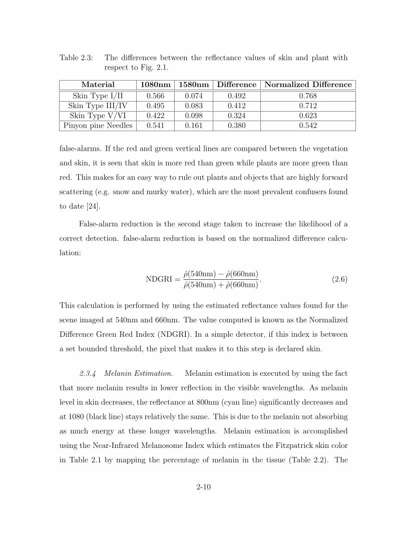
Table 2.3: The differences between the reflectance values of skin and plant withrespect to Fig. 2.1.

Material 1080nm 1580nm Difference Normalized Difference

Skin Type I/II 0.566 0.074 0.492 0.768Skin Type III/IV 0.495 0.083 0.412 0.712Skin Type V/VI 0.422 0.098 0.324 0.623

Pinyon pine Needles 0.541 0.161 0.380 0.542

false-alarms. If the red and green vertical lines are compared between the vegetation

and skin, it is seen that skin is more red than green while plants are more green than

red. This makes for an easy way to rule out plants and objects that are highly forward

scattering (e.g. snow and murky water), which are the most prevalent confusers found

to date [24].

False-alarm reduction is the second stage taken to increase the likelihood of a

correct detection. false-alarm reduction is based on the normalized difference calcu-

lation:

NDGRI =ρ(540nm)− ρ(660nm)

ρ(540nm) + ρ(660nm). (2.6)

This calculation is performed by using the estimated reflectance values found for the

scene imaged at 540nm and 660nm. The value computed is known as the Normalized

Difference Green Red Index (NDGRI). In a simple detector, if this index is between

a set bounded threshold, the pixel that makes it to this step is declared skin.

2.3.4 Melanin Estimation. Melanin estimation is executed by using the fact

that more melanin results in lower reflection in the visible wavelengths. As melanin

level in skin decreases, the reflectance at 800nm (cyan line) significantly decreases and

at 1080 (black line) stays relatively the same. This is due to the melanin not absorbing

as much energy at these longer wavelengths. Melanin estimation is accomplished

using the Near-Infrared Melanosome Index which estimates the Fitzpatrick skin color

in Table 2.1 by mapping the percentage of melanin in the tissue (Table 2.2). The

2-10

process begins with a ratio between estimated reflectance of 800nm and 1080nm.

N(λ) =ρ(800nm)

ρ(1080nm)(2.7)

N(λ) is used to estimate reflectance at 685nm (D per Eqn. (2.8)) which is used

to determine melanin percentage (M per Eqn. (2.9)). The constants X in Eqn. (2.8)

and C in Eqn. (2.9) are solved using a linear regression (details are provided in [23]):

D = X1N2 −X2N +X3 (2.8)

M = −C1D5 + C2D

4 − C3D3 + C4D

2 − C5D + C7 (2.9)

2.4 Geometric Optics

Geometric optics, treats light as rays and traces these rays through optical

systems to solve for important optical system properties such as image/object distance

and height, and magnification and focal length. This is a simplification of actual light

propagation, because it assumes that an object is imaged perfectly and does not take

into consideration the thickness of the lens.

2.4.1 Fundamental Calculations. Fig. 2.7 shows a single lens with an object

and its image. First, there are two “spaces” in this figure. In this case, the object

or target is on the left of the lens. As such, this is the object space, where variables

are denoted with a subscript ‘o’. To the right of the lens is the image space, where

variables are denoted with a subscript ‘i’. On the object space side, there are several

labeled quantities: So is the object distance, which is the distance that the object is

placed from the lens; Xo is the object height and in this two-dimensional case is the

distance from the optical axis to the edge of the object; and fo is the focal length

of the lens. On the image space of the figure, there are the quantities Si, Xi, and

fi. Here, Si is the image distance, which is the distance between the lens and the

image plane; Si can be negative which means a virtual image is created. If a scene

2-11

Figure 2.7: Single lens imaging geometry.

is imaged through the lens in Fig. 2.7, the plane onto which it is imaged would need

to be the image distance away for it to be in “perfect” focus. The variable Xi in this

two-dimensional case is the height of the image, which is solved for by finding the

magnification of the system. Finally, fi is the focal length of the lens. For single-lens

systems, as depicted in Fig. 2.7, the focal lengths are the same, but for systems of

more than one lens, there is a front focal length and a back focal length.

Solving for Si in a single lens setup is accomplished using:

Si =Sof

So − f. (2.10)

The magnification (M) of the system is solved using:

M =−Si

So

=Xi

Xo

(2.11)

2-12

Figure 2.8: A multiple lens setup labeled with pertinent variables.

and describes how much larger or smaller the objects in the imaged scene are than

the objects in object space. If M is negative, then the image is inverted.

A multiple-lens system is shown in Fig. 2.8. When more than one lens is used,

the terms discussed above are still valid and a new variable is added. The distance

between the lenses is important and is represented by the variable d. To find the

image distance Si2, one uses:

Si2 =f2d− f2So1f1

So1−f1

d− f2 − So1f1So1−f1

. (2.12)

The magnification is computed using:

Mt = − f1Si2

d (f1 − So1) + f1So1

. (2.13)

2.4.2 Diffraction and Aberrations. When an object is imaged through a

lens it becomes blurred and two important concepts explain why it occurs. The best

performance obtainable from an optical system is diffraction limited performance.

Diffraction theory treats lights as electromagnetic waves, where geometric optics is

the limit in which the wavelength approaches zero. Because light is treated as a

wave in diffraction theory it can “bend” around apertures and objects. When light

2-13

passes through a circular aperture it is blurred out into an “Airy Disk” pattern which

is mathematically modeled by a Bessel function. To solve for the diameter of the

central lobe of the Bessel function, where 84% of the energy is located as described

as [7] use:

dspot =2.44λf

dlens(2.14)

where the largest wavelength that the individual detector needs to see is λ, the focal

length of the lens is f , and the diameter of the lens is dlens.

As stated above, diffraction-limited is the best-case scenario, and aberrations

blur out the spot to larger sizes. Monochromatic and chromatic are the two main

categories of aberrations. These aberrations result from the shape of the lens, type of

lens, materials used in the lens, position of the lens in a system, and/or the wavelength

of the light [13].

2.5 Radiometry

Radiometry is the analysis of light energy propagating through space from a

source to a detector. It is used to model the system discussed in Chapter III to

show the amount of energy incident on a single pixel of each camera. Determining

the amount of energy incident on a pixel involves many factors including radiance

of the source, reflectivity of the target, attenuation of the light by the atmosphere,

distance to detector, and the transmission properties of the optics through which

the light must pass. Figure 2.9 shows the steps necessary to model the system from

illumination source to focal plane array.

2.5.1 Solid Angle. An important concept to understand in radiometry is

solid angle, measured in steradians. This is the three-dimensional counterpart of the

planar angle, measured in radians. Beginning with the definition of radian measure,

2-14

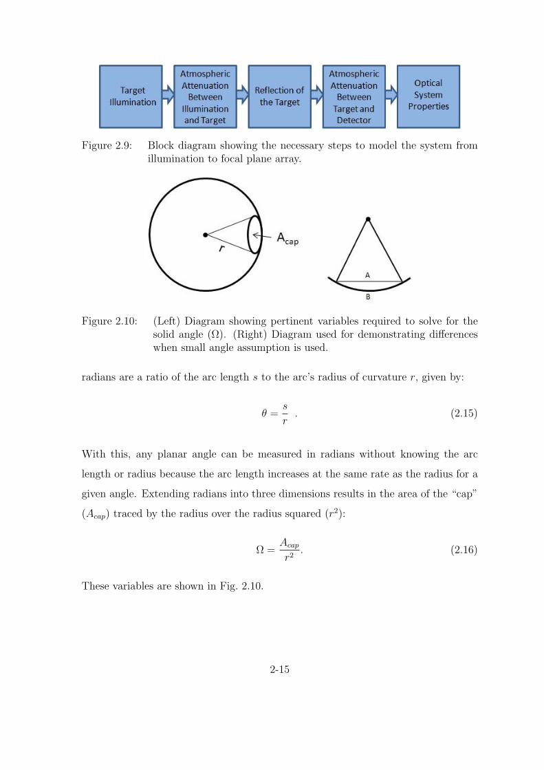
Figure 2.9: Block diagram showing the necessary steps to model the system fromillumination to focal plane array.

Figure 2.10: (Left) Diagram showing pertinent variables required to solve for thesolid angle (Ω). (Right) Diagram used for demonstrating differenceswhen small angle assumption is used.

radians are a ratio of the arc length s to the arc’s radius of curvature r, given by:

θ =s

r. (2.15)

With this, any planar angle can be measured in radians without knowing the arc

length or radius because the arc length increases at the same rate as the radius for a

given angle. Extending radians into three dimensions results in the area of the “cap”

(Acap) traced by the radius over the radius squared (r2):

Ω =Acap

r2. (2.16)

These variables are shown in Fig. 2.10.

2-15

When r2 >> Acap, Acap can be approximated as a chord (line A in Fig. 2.10),

rather than taking the curvature into account (line B in Fig. 2.10). This small angle

approximation is used throughout the radiometric calculations in this thesis.

2.5.2 Defining Radiometric Quantities. To facilitate discussion, we first

describe the variables and their units. When radiometric quantities are represented

with watts, they are called joule or energy units and are given the subscript, e.

When the radiometric quantities are represented with photons per second, they are

called photon units and are given the subscript, p. Radiometric calculations are

represented spectrally or totally. Spectral representation yields a calculated quantity

per wavelength (µm, nm). When the units are given in total, it means that the spectral

measurements have been integrated over a certain region of wavelengths. When the

measurements are represented spectrally, they can be converted between the energy

and photon units. The conversion can only be accomplished when the measurements

are spectral, because the conversion is wavelength-dependent, as illustrated:

EnergyQuantity(λ) = PhotonQuantity(λ)hc

λ(2.17)

where h is Planck’s constant, c is the speed of light, and λ is the wavelength.

A light ray is often described by the energy it contains (Q) and the rate of the

energy received (the flux, Φ) which is a measurement of the light ray’s power. The

most easily understood radiometric quantities are those that involve flux density, such

as irradiance (E) and exitance (M) which are flux per unit area either incoming or

outgoing, respectively. The next quantity of interest is intensity (Ie) which is flux per

unit solid angle.

The most fundamental quantity is radiance as the other quantities are derived

directly from it. Radiance is defined as the amount of power radiated per unit pro-

jected source area per unit sold angle [7]. Table 2.4 shows the International System

of Units (SI) for the radiometric quantities used in this thesis.

2-16

Table 2.4: Radiometric QuantitiesEnergy Units Photon Units

Quantity Symbol Units Symbol UnitsEnergy Qe joule Qp photon

Flux Φe watt Φpphoton

s

Intensity Iewattsr

Qpphotons sr

Exitance Mewattcm2 Mp

photons cm2

Irradiance Eewattcm2 Ep

photons cm2

Radiance Lewattsr cm2 Lp

photons sr cm2

Figure 2.11: Diagram showing locations of θd and θs.

2.5.3 Solving for Radiometric Quantities. Since the small-angle approxima-

tion is assumed, the radiance (L) can be written in its non-differential form:

L =Φ

Ascos (θs) Ωd

(2.18)

where Φ is the flux from the source, As is the area of the source, Ωd is the solid angle

subtended by the detector, and θs is the angle formed by the normal to the source and

the optical path. Figure 2.11 shows θs and later mentioned θd in a diagram to show

their locations. (For the purpose of showing how the quantities can be computed,

neither photon or joule units are explicitly specified.)

From the radiance (L) in Eqn. (2.18), the flux (Φ) is computed by:

Φ = LAscos (θs) Ωd . (2.19)

2-17

From flux (Φ), the intensity (I) and exitance (M) are solved for as:

I =Φ

Ωd

= Lcos (θs)As and (2.20)

M =Φ

As

= Lcos (θs) Ωd . (2.21)

To find the irradiance (E), the solid angle (Ωd) is divided into its constituent compo-

nents:

Ωd =Adcos (θd)

R2and (2.22)

E =Φ

Ad

=Lcos (θd) cos (θs)As

R2. (2.23)

The second important assumption is that the source is lambertian. This means that

the source’s radiance (L) is independent of the viewing angle (θs). Under this as-

sumption, the relationship between radiance (L) and exitance (M) is:

M = πL . (2.24)

2.5.4 Modeling Illumination Sources. The radiance of a source is represented

as a blackbody source. This type of source emits radiation at the theoretical maximum

with respect to the source temperature and the wavelength. The expression for joule

radiance (Le) is:

Le(λ, T ) =2hc2

λ5(e

hcλkT − 1

) [W

cm2 − sr− nm

](2.25)

where h is Planck’s constant, c is the speed light, k is Boltzmann’s constant, and T

is the temperature in Kelvin.

Figure 2.12 shows the blackbody curves for three different temperatures. The

highest temperature modeled is that of the sun, 5950K (red). The 4500K temperature

(green) is an intermediate step to show how the curves progress as the temperature

2-18

0 500 1000 1500 2000 2500 3000

0.0

0.5

1.0

1.5

2.0

2.5

3.0

Λ HnmL

Rad

ianc

eHWc

m2-

Sr-

nmL

3200K

4500K

5950K

Temperature

Figure 2.12: Three radiance blackbody curves with varying temperatures. The sunis shown in the red curve with a temperature of 5950K. The 4500Ktemperature, in green, is an intermediate step to show how the curvesprogress as the temperature changes. The ASD Pro Lamps used inthe study is represented with a 3200K black body curve.

changes. The color temperature of the lamps used in Chapter IV for the indoor

study are 3200K. Because the lamps are not perfect blackbody radiators, (so-called

graybodies), the color temperature given is used to model the blackbody curve of the

source [7].

2.5.5 Atmospheric Attenuation. The atmospheric transmission is an impor-

tant aspect to make the model as realistic as possible. The amount of attenuation

the atmosphere has on an illumination source is dependant on the distance it has to

travel. All the other atmospheric properties are taken into consideration in the extinc-

tion plot, shown in Fig. 2.131. It is made for winter WPAFB atmosphere with default

visibility (∼17km) in climatological aerosols. The extinction coefficient is transformed

1This plot was created by Dr. Steven Fiorino, Atmospheric Physicist, with Laser EnvironmentalEffects Definition and Reference (LEEDR).

2-19

400 600 800 1000 1200 1400 1600 18000

20

40

60

80

100

120

140

Wavelength (nm)

Ext

inct

ion

(km

−1 )

Figure 2.13: Atmospheric extinction created in Laser Environmental Effects Defi-nition and Reference (LEEDR). This is used along with beer’s law toestimate atmospheric transmission.

into atmospheric transmission using Beer’s law:

τ(λ) = e−α(λ)ℓ (2.26)

where α(λ) is the spectral extinction in Fig. 2.13 and ℓ is the distance in km between

the source and detector. Two examples of using Beer’s law and how atmospheric

transmission changes with respect to distance are shown in Fig. 2.14.

2.5.6 Converting Photons to Electrons. Once the light from the illumina-

tion source passes through the atmosphere and is reflected off the target, additional

attenuation occurs due to the system components. Every lens, mirror, and filter has a

transmission that needs to be taken into account to model the system appropriately.

Since the end goal is to model the data numbers for each image, the number of pho-

tons that create electrons needs to be determined. This count of photons is directly

related to the data numbers. Once the energy values at each pixel are in photons per

2-20

400 600 800 1000 1200 1400 16000

0.2

0.4

0.6

0.8

1

Wavelength (nm)

Atm

osph

eric

Tra

nsm

issi

on

400 600 800 1000 1200 1400 16000

0.2

0.4

0.6

0.8

1

Wavelength (nm)

Atm

osph

eric

Tra

nsm

issi

onFigure 2.14: Two examples of using Beer’s law and how atmospheric transmission

changes with respect to distance. (Left) Distance between detectorand source 2km. (Right) Distance between detector and source 10km.

second, they are multiplied by the integrations times of the cameras to determine how

many photons are hitting the array in each frame. To determine how many photons

create electrons on average, the quantum efficiency of each camera is used. Dereniak

defines quantum efficiency as the efficiency of converting a photon to an electron, or

the number of independent electrons produced per photon [7].

2.6 Summary

First, the background necessary to understand the features exploited and meth-

ods used for skin detection which are necessary to build the system are discussed.

Second, the reflectance properties of human skin are discussed to give the reader a

basis of why certain wavelengths were chosen. The algorithms used to perform the

detections are discussed to show how the images are processed. Third, an overview of

the geometric optics used to solve for lens focal lengths and diameters is completed.

Lastly, a radiometry overview is accomplished to discuss how the model is created for

2-21

this thesis. Now that the background is reviewed the methodology behind designing

the system and the model are discussed.

2-22

Figure 3.1: Block diagram for the monocular skin detection, melanin estimation,and false-alarm suppression camera system developed in this thesis.

III. Methodology

The construction of the system is based on the essential components depicted in

Fig. 3.1: detectors, fore optic, secondary lenses, iris diaphragms, dichroic mirrors,

and filters. The remainder of the chapter describes and characterizes each component

in the system depicted in Fig. 3.1. Near-infrared (NIR) and visible (VIS) cameras are

necessary to do the skin detection, melanin estimation, and false-alarm suppression.

The specifications necessary and the chosen cameras are discussed. Lenses need to be

chosen for the fore optic and correcting lenses. The beamsplitters’ size and transmis-

sion are discussed. The transmission of the filters used to narrow down the broadband

energy are discussed as well.

3.1 Camera Selection

As discussed early in Section 2.1, this system requires NIR and VIS wavelengths

to perform the necessary detection, false-alarm suppression, and melanin estimation

tasks. These cameras need to record at least 1fps with an external trigger so every

camera can image the scene at the same time. The goal is to find cameras that have

3-1

Table 3.1: Specifications for the Goodrich SU640KTSX-1.7RT.Parameter Value

Spectral Response 900nm-1700nmPixel Pitch 25µm

Array Format 640× 512Image Depth 12 bitFrame Rate 30fps

Camera Body Size(H × W × D) 2.1in× 2.1in× 2.55in

the capability to do 30fps as the algorithm speed increases. High spatial resolution is

another important aspect needed to detect a person from ∼710ft away. In Fig. 3.1,

the VIS cameras are Camera 1 and Camera 2 and the NIR cameras are Camera 3

and Camera 4.

3.1.1 Near-Infrared Cameras. A limited number of InGaAs near-infrared

(NIR) cameras are available commercially. We chose the Goodrich SUI640KTSX-

1.7RT High Sensitivity InGaAs NIR Cameras due to performance characteristics and

compact size. As such, the design of the system is based on them. Table 3.1 shows the

specifications of the Goodrich camera relevant to this thesis. The camera response in

Fig. 3.2 was experimentally measured with the use of an Oriel Lamp and a calibrated

monochromator. To make sure the camera is not saturating the images used to create

the plot are checked for data number values of 4095. The absorption feature at

1380nm is due to atmospheric water absorption [29]. From Fig. 3.2, one can see that

the skin detection bands at 1080 and 1580nm are well within the camera’s response,

as indicated with the vertical lines.

3.1.2 Visible Cameras. Since false-alarm reduction uses 540nm (green line

in Fig. 2.1) and 680nm (red line in Fig. 2.1), as specified in Section 2.1, a common

visible camera is used. There were a few approaches used to find a camera that

works for the false-alarm suppression. The first approach is to find a visible camera

that has the same pixel size as the Goodrich Cameras. This makes the pixel-by-pixel

comparison for the detection task simple. Since the Goodrich cameras have 25µm

3-2

200 400 600 800 1000 1200 1400 1600 1800 2000 22000.1

0.2

0.3

0.4

0.5

0.6

0.7

0.8

0.9

1

Wavelength (nm)

Rel

ativ

e R

espo

nse

Figure 3.2: Relative response of the Goodrich SU640KTSX-1.7RT High Sensitiv-ity InGaAs short wave infrared camera. The absorption feature at1380nm is due to atmospheric water absorption. Skin detection bandsare marked with vertical lines.

pixels, the other system cameras need to match. Research found that it is difficult to

find 25µm pixel silicon cameras. Because one could not be located, a second approach

was necessary. This second approach attempts to find a pixel size that, when averaged

together, resulting in 25µm superpixels. For example, using a 6.25µm pixel camera

averaging 4×4 pixels would make an equivalent 25µm pixel. The trade off by grouping

pixels is that a larger focal plane array is necessary to match the Goodrich camera’s

640×512 array. Table 3.2 shows how close typical pixel sizes are grouped to estimate

25µm.

If a perfect 25µm superpixel cannot be created, the pixel grouping that is closest

should be used. The problem at first is to get this larger (or smaller) pixel to be

spatially registered with the 25µm pixel. This is fixed by moving the cameras relative

to an in focus image in order to image their pixels to the same size as the 25µm

pixels. Fig. 3.3 shows the distance a camera needs to be moved relative to where a

well focused image would appear so that the imaged pixels are 25µm pixels at 707ft.

3-3

Table 3.2: Pixel sizes used to calculate how far camera must be moved to get sameimaged size as 25µm.

Pixel Size Group Size Superpixel Size Array Size To Match 640× 512µm Pixel by Pixel µm Pixel by Pixel

7.4 3× 3 22.2 1920× 15366 4× 4 24 2560× 204812 2× 2 24 1280× 102424 1× 1 24 640× 5129 3× 3 27 1920× 1536

6.45 4× 4 25.8 2560× 20485.2 5× 5 26 3200× 2560

1.00 1.05 1.10 1.15 1.20

-10

0

10

20

Imaged Pixel Size HinchesL

Mov

emen

tReq

uire

dHm

mL

5.2Μm

6.45Μm

9Μm

6,12,24Μm

7.4Μm

Pixel Size

Figure 3.3: Distance and direction a camera needs to move so that its pixel size isthe same as the Goodrich camera. The difference is calculated from a150mm focus. Negative numbers refer to the camera moving away fromthe lens while positive is moving towards.

A negative number refers to the camera moving away from the lens, while positive is

toward the lens.

Moving the cameras could result in the image being slightly out of focus, but

with the averaging taking place, it might not make a significant difference. To theo-

retically see if the image is still in focus, a depth of focus calculation is accomplished

and shown in Fig. 3.4. As defined in [9], depth-of-focus is the amount of defocus cor-

responding to being out of focus by one quarter wavelength. This calculation uses the

3-4

4.0 4.5 5.0 5.5 6.0

0.02

0.04

0.06

0.08

0.10

f Number

Dep

thof

Focu

s+-

mm

400nm

700nm

1000nm

1500nm

Wavelength

Figure 3.4: The depth of focus calculation with respect to f -number.

Rayleigh criterion which states that if the optical path distance is less than or equal

to a quarter wavelength, then it is still considered diffraction-limited [9]. Figure 3.4

demonstrates how far each of the four cameras can move and still theoretically stay

in focus. Figure 3.4 shows the detectors can move only fractions of a mm to stay in

focus, while Fig. 3.3 shows that the detectors need to move several mm to image to

the right size. This means that the images would most likely be out of focus. As such,

the following approach is considered.

The last approach uses a second lens to image the pixels of the visible camera

to the same size pixels as the Goodrich cameras. (The lens is discussed in more detail

in the next section). The advantage of this design is that the number of cameras one

can use for the visible wavelengths is substantially extended. This extension includes

any color camera that has at least as many pixels as the Goodrich focal plane array

and that can be externally triggered. A camera that matched these specifications

is the ThorLabs DCC1645C High Resolution USB2.0 CMOS camera. A picture of

this camera is shown in Fig. 3.5 and the specifications in Table 3.3. The responsivity

provided by the vendor is shown in Fig. 3.6.

The array format works out well, because the pixels can be imaged out to half

the size of the 25µm pixels. This means that, not only can the visible camera be used

3-5

Figure 3.5: Picture of the ThorLabs High Resolution USB2.0 CMOS Series Cam-eras.

Table 3.3: Important specifications of the ThorLabs DCC1645C.Parameter Value

Spectral Response Visible lightFormat RGB

Pixel Pitch 3.6µmArray Format 1280× 1024Image Depth 10 bitFrame Rate 25fps

Camera Body Size(H × W × D) 1.88in× 1.68in× 1.00in

for the false-alarm reduction discussed above, it provides a higher resolution image of

the imaged scene. These higher resolution snapshots can be triggered and saved by

the user or whenever skin is detected. The small size of this camera is additionally

important since there is little room to fit the four cameras required for this system.

Due to the reasons discussed above, a second ThorLabs camera is chosen for the

melanin estimation. Since RGB is not necessary for the melanin estimation task, the

DCC1545M High Resolution USB2.0 CMOS monochrome camera is chosen. Table 3.4

shows the specifications for the camera and the responsivity given by the vendor is

shown in Fig. 3.7. (Note that the response of the DCC1645C is better than that of

3-6

Figure 3.6: Relative Response of the ThorLabs DCC1645C.

the DCC1545M at 800nm. However the DCC1645C has an IR cut filter built into the

camera while the DCC1545M does not.)

3.2 Lens Selection

The complete system requires three lenses. The first is a 150mm focal length

lens used as the single fore optic (Fore Optic in Fig. 3.1). The second lens (Lens 1

Table 3.4: Important specifications of the ThorLabs DCC1545M.Parameter Value

Spectral Response Visible lightFormat Monochrome

Pixel Pitch 5.2µmArray Format 1280× 1024Image Depth 10 bitFrame Rate 25fps

Camera Body Size(HxWxD) 1.88in x 1.68in x 1.00in

3-7

Figure 3.7: Relative Response of the ThorLabs DCC1545M. Even though the plotshows an IR cut filter this camera model does not have one.

in Fig. 3.1) is placed in front of the ThorLabs RGB camera correcting for its pixel

size difference. The third lens (Lens 2 in Fig. 3.1) is placed in front of the ThorLabs

monochrome camera to correct for its pixel size difference. Due to the specifications

described in Section 1.1, the lenses were selected to image the pixels of each camera

to no larger than 2× 2 inches at 707ft.

3.2.1 Fore Optic (Front Lens). Proper selection of the fore optic is difficult

as there are several considerations one must balance. First, as stated above, the pixels

of each camera need to be imaged to at most 2 × 2 inches to get the largest FOV

without losing spatial resolution. Second, the image distance needs to be large enough

to fit the three dichroic mirrors between the cameras. Lastly, the system needs to be

kept as close to diffraction-limited as possible.

Because the object distance is relatively far away, the focal length is approx-

imately the same as the image distance. Figure 3.8 shows the image distance with

3-8

1.0 1.2 1.4 1.6 1.8 2.0

120

140

160

180

200

Imaged Pixel Size HInchesL

Imag

eD

ista

nceHm

mL

Figure 3.8: The image distance with respect to imaged pixel size for a 25µm pixelcalculated with the object distance set at 707ft.

respect to the size of the imaged pixel for an object imaged at 707ft. As seen in

Fig. 3.8, a 2× 2 inch imaged pixel results in an image distance of 106.1mm (4.18in).

This distance is far too small for the placement of the required dichroic mirrors behind

the lens (as shown previously in Fig. 3.1). For more space between the lens and the

cameras, the imaged pixel must be smaller as indicated in Fig. 3.8.

The mirrors sizes are designed to support up to a 50mm diameter lens. The final

solution has three different sized mirrors in the chain and is discussed in more detail

in Section 3.3. To make sure there is enough room to fit all the mirrors with holders,

each mirror is considered the same size, so a focal length of 150mm is necessary to

image onto the final camera in the chain (see Fig. 3.9). Using the 150mm focal length

and object distance of 707ft, the imaged pixel size decreases to 1.41in, which increases

the spatial resolution of the camera. Figures 3.10 and 3.11 show how many more “pure

pixels” are seen by the cameras with the 1.41in imaged pixel size. The figures are

to scale and the same head and hand size are used as described in Table 1.1. An

increase from 7 to 18 pixels on the head and 6 to 8 pixels on the hand show that the

smaller pixel size benefits the detection. Because this lens is directly imaging onto the

Goodrich camera, its diffraction-limited spot diameter needs to be less than 25µm.

3-9

Figure 3.9: System setup assuming the three dichroic mirrors are the same sizein order to approximate the minimum focal length that leaves enoughroom for the mirrors. All blue arrows are 50mm in length.

Figure 3.10: To scale 1.41in pixels corresponding to the measured head and handsize. This shows the best case scenario with the pure skin pixels shownin red.

Using the lens specifications in Table 3.5 and Eqn. (2.14) the diffraction spot size is

solved as 15.37µm, which meets the requirement.

Off-the-shelf optics are used for the monocular skin detection system developed

in this thesis. The Newport PAC075 achromatic doublet met the previously stated

requirements and is chosen for the fore optic. An achromatic doublet is used because

it is made to correct for the refraction differences in the visible spectrum. The visible

light energy is the broadest spectrum sent to one camera, so the largest chromatic

aberrations occur here. The other cameras receive smaller spectral bands so chromatic

3-10

Figure 3.11: To scale 1.41in pixels corresponding to the measured head and handsize. This shows the worst case scenario with the pure skin pixelsshown in red.

Table 3.5: Specifications of the PAC075 Newport Achromatic Double lens.Parameter Value

Airy Disc Size @ 1.6µm 15.37µmFocal Length 150mm

Diameter of Optic 38.1mmf/# 3.93

aberrations should affect their images less. The specifications of the Newport Optics

lens is shown in Table 3.5.

3.2.2 Color Camera Lens. There are two choices of magnification for the

ThorLabs cameras to make a pixel-by-pixel comparison possible with the Goodrich

cameras. The pixels from the ThorLabs cameras can be imaged the same size as the

Goodrich cameras, or they can be imaged smaller to have a higher spatial resolution.

Due to the array format of the camera, discussed in Section 3.1, there are enough pixels

to image with twice the spatial resolution and still have the same FOV. This results

in a 4:1 pixel ratio between the ThorLabs and Goodrich cameras. The specifications

that need to be determined are the distance between the fore optic and this second

3-11

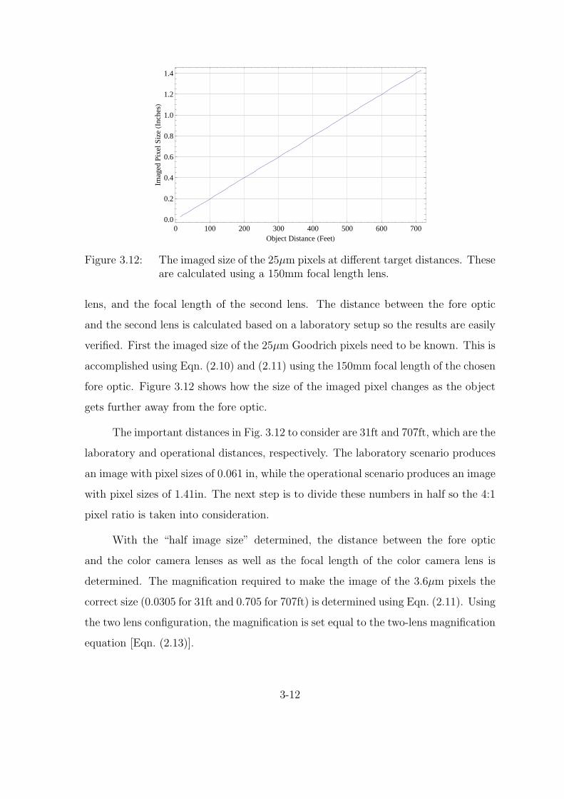
0 100 200 300 400 500 600 7000.0

0.2

0.4

0.6

0.8

1.0

1.2

1.4

Object Distance HFeetL

Imag

edPi

xelS

izeHI

nche

sL

Figure 3.12: The imaged size of the 25µm pixels at different target distances. Theseare calculated using a 150mm focal length lens.

lens, and the focal length of the second lens. The distance between the fore optic

and the second lens is calculated based on a laboratory setup so the results are easily

verified. First the imaged size of the 25µm Goodrich pixels need to be known. This is

accomplished using Eqn. (2.10) and (2.11) using the 150mm focal length of the chosen

fore optic. Figure 3.12 shows how the size of the imaged pixel changes as the object

gets further away from the fore optic.

The important distances in Fig. 3.12 to consider are 31ft and 707ft, which are the

laboratory and operational distances, respectively. The laboratory scenario produces

an image with pixel sizes of 0.061 in, while the operational scenario produces an image

with pixel sizes of 1.41in. The next step is to divide these numbers in half so the 4:1

pixel ratio is taken into consideration.

With the “half image size” determined, the distance between the fore optic

and the color camera lenses as well as the focal length of the color camera lens is

determined. The magnification required to make the image of the 3.6µm pixels the

correct size (0.0305 for 31ft and 0.705 for 707ft) is determined using Eqn. (2.11). Using

the two lens configuration, the magnification is set equal to the two-lens magnification

equation [Eqn. (2.13)].

3-12

Figure 3.13: This figure demonstrates a safe distance between the fore optic andcorrecting lenses so they will not hit the mirrors.

To make sure the second lens does not hit the mirrors, it needs to be at least

2.2in from the front lens (see system layout in Fig. 3.13). Figure 3.14 shows what focal

lengths are necessary to maintain the proper magnification and the resulting image

distance as the distance between the lenses is varied. A 30mm focal length lens does

not hit the mirror and leaves enough room to move the lens closer to image targets

further away than 707feet. Using a 30mm focal length, the distances between the

fore optic and the second lens are 3.08in for a target 31ft away (red line) and 2.98in

for a target 707ft away (blue line). These target distances result in image distances

of 0.841 and 0.843in, respectively. This shows that for any operational distance at

which the object is placed, the distance necessary for the lenses and cameras to move

is relatively small. This keeps the system compact for a wide variety of scenarios for

which it might be used.

The LB1757-A Bi-Convex Lens from ThorLabs is chosen for this camera. The

specifications of the lens are shown in Table 3.6. As Fig. 3.15 demonstrates, the

coating on this lens is specifically designed for efficiently transmitting 425-675nm

wavelengths at >96.7%.

3.2.3 Monochrome Camera Lens. To ensure that the lens for the monochrome

camera does not hit the second dichroic mirror, the distance needs to be at least 4.08in

3-13

2.5 3.0 3.5 4.020

25

30

35

Distance Between Lenses HInchLFo

calL

engt

hR

equi

redHm

mL

2.5 3.0 3.5 4.0

0.6

0.7

0.8

0.9

1.0

1.1

Distance Between Lenses HInchL

Imag

eD

ista

nceHI

nchL

Figure 3.14: (Top) This plot shows what distances between lenses and focal lengthsare necessary to get the proper magnification of the pixels. (Bottom)Image Distance of two lens optical chain. (Red) Object 31ft away fromfront lens. (Blue) Object 707ft away from front lens.

from the fore optic. This is shown in the system layout diagram, Fig. 3.13. Figure 3.16

shows what focal lengths are necessary to maintain the proper magnification and the

resulting image distance as the distance between the lenses is varied. A 30mm focal

length lens does not hit the mirror and leaves enough room to move the lens closer to

image targets further away than 707feet. Using a 30mm focal length, the distances

between the fore optic and the second lens are 4.34in for a target 31ft away (red line)

and 4.25in for a target 707ft away (blue line). These target distances both result

in image distances of 0.69in. This shows that for any operational distance at which

the object is placed, the distance necessary for the lenses and cameras to move is

relatively small. This keeps the system compact for a wide variety of scenarios for

which it might be used.

3-14

Table 3.6: Specifications of the ThorLabs LB1757-A Lens.Parameter Value

Focal Length 30.0mmDiameter 25.4mm

F# 1.18Glass BK7

Coatings Anti-reflective Visible

400 600 800 1000 1200 1400 1600 18000.65

0.7

0.75

0.8

0.85

0.9

0.95

1

Per

cent

Tra

nsm

issi

on

Wavelength (nm)

Figure 3.15: Transmission of the ThorLabs LB1757 A coated lens measured byThorLabs using a spectrophotometer.

The LB1757-B Bi-Convex Lens from ThorLabs is chosen for this camera. The

specifications of the lens are shown in Table 3.7. As Fig. 3.17 demonstrates, the

coating on this lens is specifically designed for efficiently transmitting 775-825nm

wavelengths at >98.57%.

3.3 Dichroic Mirrors

Figure 3.1 shows the location of the dichroic mirrors in the system. These

mirrors are designed specifically to properly divide the spectrum for use in this system.

The reflection and transmission properties of the specified wavelengths need to be as

high as possible so that detections can be accomplished even under low illumination

3-15

4.0 4.2 4.4 4.6 4.8 5.0

20

25

30

35

Distance Between Lenses HInchLFo

calL

engt

hR

equi

redHm

mL

4.0 4.2 4.4 4.6 4.8 5.0

0.4

0.5

0.6

0.7

0.8

Distance Between Lenses HInchL

Imag

eD

ista

nceHI

nchL

Figure 3.16: (Top) This plot shows what distances between lenses and focal lengthsare necessary to get the proper magnification of the pixels. (Bottom)Image Distance of the two-lens optical chain. (Red) Object 31ft awayfrom front lens. (Blue) Object 707ft away from front lens.

situations. Different light division methods were considered, most were not efficient

enough for use in skin detection, due mostly to the already low solar illumination at

1580nm. If the system is only used during bright days, then off-the-shelf cold mirrors

and pellicles might work adequately. For this research, we wanted to push the search

and rescue capability to its limits, so we chose to use dichroic mirrors.

The mirrors need to meet two size specifications. First, the mirrors need to

reflect the entire image from the lens since this system supports at most a 50mm lens.

Second, the mirrors must fit in the 150mm (∼6in) space between the fore optic and

Camera 4. Fig. 3.18 shows the model of the system tracing relevant rays of light.

To meet the specifications above, the mirrors need to be 2.9, 2.2 and 2.0in

squares. Furthermore the mirrors need to allow all polarizations to transmit and

3-16

Table 3.7: Specifications of the ThorLabs LB1757-B Lens.Specification Value

Focal Length 30.0mmDiameter 25.4mm

F# 1.18Glass BK7

Coatings Anti-reflective NIR

400 600 800 1000 1200 1400 1600 18000.7

0.75

0.8

0.85

0.9

0.95

1

Per

cent

Tra

nsm

issi

on

Wavelength (nm)

Figure 3.17: Transmission of the ThorLabs LB1757 B coated lens measured byThorLabs using a spectrophotometer.

reflect respectively. (Skin detection does not necessarily require polarized light to work

and this aspect has not been researched to date). Table 3.8 shows the wavelengths

reflected and transmitted with respect to each mirror. These bands are large so

that future studies can determine the effect different width bandpass filters have on

performance in terms of probability of detection and false-alarms, as well as accuracy

in skin color estimation.

Figures 3.19 - 3.21 are the measured mirror responses. The mirrors are measured

in the same 45 orientation as they would be in the actual system. The green regions

show the spectra that need to be reflected and red regions show the spectra that need

to be transmitted by each mirror. The high reflection and transmission efficiencies are

3-17

Figure 3.18: Block diagram of the system with references for the path of the light.

needed to use the skin detection system in low-lighting conditions. It is also important

to note that the mirrors are directional with respect to reflected image quality.

3.4 Filters

To reduce the spectral content to those specified in [23], filters are used. The

filters need to have high transmission so as not to negate the high percentage of in-

cident energy the mirrors reflect or transmit. The camera used for the 1080nm band

has two modes of use. The spectrum it sees can be that reflected by the respective

mirror or the mirror and a filter (a Semrock FF01-1060/13-25). The Semrock FF01-

1060/13-25 filter has a transmission of >90% for 13nm centered around 1060nm, as

3-18

Table 3.8: Wavelength transmission and reflection bands for mirrors 1, 2, and 3shown in Fig. 3.1. CW is the center wavelength of the band .

Reflected TransmittedMirror Total CW Bandwidth Total CW Bandwidth

(nm) (nm) (nm) (nm) (nm) (nm)

1 425-675 550 250 All Other Wavelengths2 775-825 800 50 All Other Wavelengths3 1030-1130 1080 100 1525-1625 1575 100

400 600 800 1000 1200 1400 16000

0.1

0.2

0.3

0.4

0.5

0.6

0.7

0.8

0.9

1

Wavelength (nm)

Tra

nsm

ittan

ce

Figure 3.19: Measured transmittance for Mirror 1. Green represents the relevantreflected spectra and red represents the relevant transmission spectrafor the skin detection, melanin estimation, and false-alarm suppressiontasks. The mirrors are measured in the same 45 orientation as theywould be in the actual system.

shown in Fig. 3.22. The filter needs to work in conjunction with the mirror, because

it transmits wavelengths that are not useful in detection. The camera used for the

1580nm band has three reasonable configurations; no filter, a Semrock bandpass filter

(NIR01-1570/3-25), or a Reynard longwave pass filter (R01718-00). The Semrock

3-19

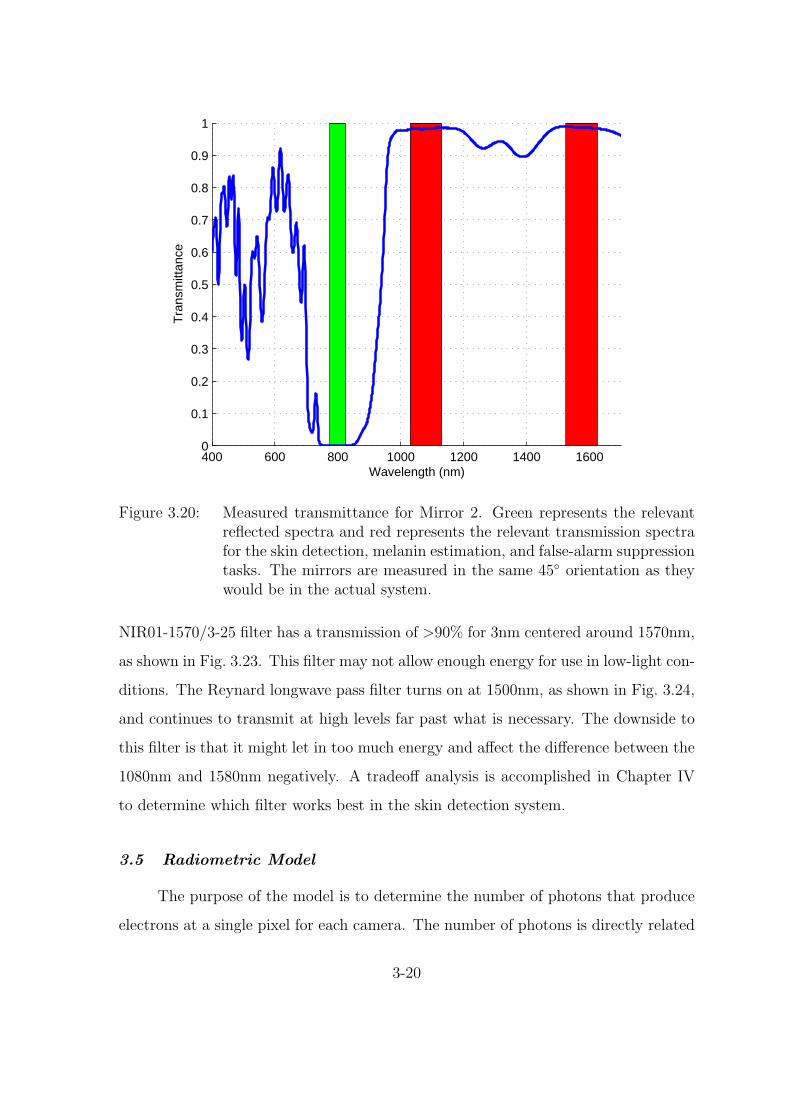
400 600 800 1000 1200 1400 16000

0.1

0.2

0.3

0.4

0.5

0.6

0.7

0.8

0.9

1

Wavelength (nm)

Tra

nsm

ittan

ce

Figure 3.20: Measured transmittance for Mirror 2. Green represents the relevantreflected spectra and red represents the relevant transmission spectrafor the skin detection, melanin estimation, and false-alarm suppressiontasks. The mirrors are measured in the same 45 orientation as theywould be in the actual system.

NIR01-1570/3-25 filter has a transmission of >90% for 3nm centered around 1570nm,

as shown in Fig. 3.23. This filter may not allow enough energy for use in low-light con-

ditions. The Reynard longwave pass filter turns on at 1500nm, as shown in Fig. 3.24,

and continues to transmit at high levels far past what is necessary. The downside to

this filter is that it might let in too much energy and affect the difference between the

1080nm and 1580nm negatively. A tradeoff analysis is accomplished in Chapter IV

to determine which filter works best in the skin detection system.

3.5 Radiometric Model

The purpose of the model is to determine the number of photons that produce

electrons at a single pixel for each camera. The number of photons is directly related

3-20

400 600 800 1000 1200 1400 16000

0.1

0.2

0.3

0.4

0.5

0.6

0.7

0.8

0.9

1

Wavelength (nm)

Tra

nsm

ittan

ce

Figure 3.21: Measured transmittance for Mirror 3. Green represents the relevantreflected spectra and red represents the relevant transmission spectrafor the skin detection, melanin estimation, and false-alarm suppressiontasks. The mirrors are measured in the same 45 orientation as theywould be in the actual system.

to the numbers that an application such as MATLABr would use to display an

image. Because a normalized difference is used to perform the detections, the photon

count can be compared in the same way to see if a detection is made. Different target

reflections are easily incorporated into the model to simulate plants, snow, or other

objects of interest. This is useful in determining detector thresholds giving the best

balance between high detections and low false-alarms.

3.5.1 Indoor Scenario Radiometry. The indoor model is used to test a

shorter range scenario where the amount of light incident on the target is easily

controlled. Figure 3.25 shows the test layout where Θd = 15, Rlamptotarget = 20ft,

and Rtargettolens = 31ft. All the components are on the same plane in the z-direction

3-21

400 600 800 1000 1200 1400 16000

0.1

0.2

0.3

0.4

0.5

0.6

0.7

0.8

0.9

1

Wavelength (nm)

Tra

nsm

issi

on

Figure 3.22: Measured transmission of the Semrock FF01-1060/13-25 NIR band-pass filter at normal incidence.

except for Lamp 3 in which Θd is a depression angle. The three illumination sources

in Fig. 3.25 are Analytical Spectral Devices (ASD) pro lamps. These lamps have an

adjustable field of view of 13-50 degrees and use a (JCV14.5V-50WC) 50 watt lamp

with a color temperature of 3200 Kelvin [19].

First, the radiance of the lamp is determined using the blackbody formula spec-

ified in Eqn. (2.25) with a temperature of 3200 Kelvin, shown in Fig. 3.26. Next, the

irradiance of the lamps on the target is determined with:

Ee [λ] =Le [λ] cos (θd) cos (θs)Asτatm

Rlamptotarget2

(3.1)

=Le [λ] cos (15

) 6.54τatm609.62

3-22

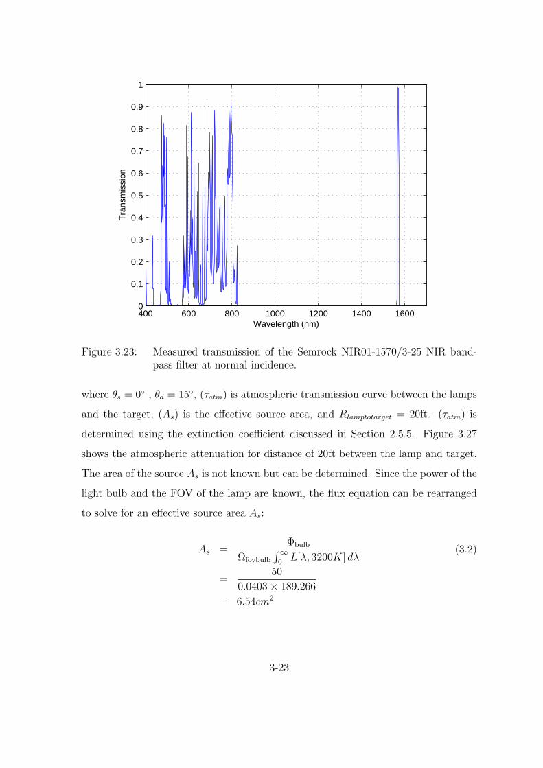
400 600 800 1000 1200 1400 16000

0.1

0.2

0.3

0.4

0.5

0.6

0.7

0.8

0.9

1

Wavelength (nm)

Tra

nsm

issi

on

Figure 3.23: Measured transmission of the Semrock NIR01-1570/3-25 NIR band-pass filter at normal incidence.

where θs = 0 , θd = 15, (τatm) is atmospheric transmission curve between the lamps

and the target, (As) is the effective source area, and Rlamptotarget = 20ft. (τatm) is

determined using the extinction coefficient discussed in Section 2.5.5. Figure 3.27

shows the atmospheric attenuation for distance of 20ft between the lamp and target.

The area of the source As is not known but can be determined. Since the power of the

light bulb and the FOV of the lamp are known, the flux equation can be rearranged

to solve for an effective source area As:

As =Φbulb

Ωfovbulb

∫∞0

L[λ, 3200K] dλ(3.2)

=50

0.0403× 189.266

= 6.54cm2

3-23

400 600 800 1000 1200 1400 16000

0.1

0.2

0.3

0.4

0.5

0.6

0.7

0.8

0.9

1

Wavelength (nm)

Tra

nsm

issi

on

Figure 3.24: Measured transmission of the Reynard Corporation R01718-00 longwave pass filter at normal incidence.

Figure 3.25: Top down view of the physical indoor setup for system testing where,θd = 15 for each lamp and Rtargettolens = 31ft. Lamp three’s θd is adepression angle.

3-24

400 600 800 1000 1200 1400 16000

0.02

0.04

0.06

0.08

0.1

0.12

0.14

Wavelength (nm)

Radia

nce

W

cm

2−

Sr−

nm

Figure 3.26: Blackbody radiance curve for a single ASD pro lamp.

400 600 800 1000 1200 1400 1600 18000.4

0.5

0.6

0.7

0.8

0.9

1

Wavelength (nm)

Atm

osph

eric

Tra

nsm

issi

on

Figure 3.27: The atmospheric transmission for a 20ft distance between the lampsand target.

where the FOV used in calculating Ωfovbulb is 13, which is the ASD Pro Lamp’s

smallest FOV. The flux of each bulb (Φbulb) is the light’s rated power, 50 W. The

resulting irradiance is solved and shown in Fig. 3.28.

3-25

400 600 800 1000 1200 1400 1600 18000

1

2

3

4

5

6

7

8x 10

−6

Irradia

nce

W

cm

2−

nm

Wavelength (nm)

Figure 3.28: The modeled irradiance on the target from three lamps.

To find the reflected exitance of the target, the irradiance is multiplied by the

target reflectance:

Me [λ] = Ee [λ] ρtarget [λ] , (3.3)

in this case human skin. Because the source is assumed lambertian, determining the

radiance is achieved by dividing by π:

Le [λ] =Me [λ]

π. (3.4)

(Note that skin is nearly lambertian when the illumination source is perpendicular to

the skin. [20]) Figures 3.29 and 3.30 show the spectral exitance and radiance respec-

tively of the target.

3.5.2 Modeling the Physical System. With the radiance of the target known,

the amount of electron forming photons at an individual pixel is:

3-26

400 600 800 1000 1200 1400 1600 18000

0.5

1

1.5

2

2.5

3

3.5

4

4.5x 10

−6

Wavelength (nm)

Exit

ance

W

cm

2−

nm

Figure 3.29: The modeled exitance of the target for TypeI/II skin.

400 600 800 1000 1200 1400 1600 18000

0.2

0.4

0.6

0.8

1

1.2

1.4x 10

−6

Wavelength (nm)

Radia

nce

W

cm

2−

Sr−

nm

Figure 3.30: The modeled radiance of the target for TypeI/II skin.

Φp−pixel =

∫ 1700nm

400nm

Le−target Ωpixel Aopt τatm τoptics−filtersλ

hcτint η dλ (3.5)

where

3-27

• Le−target(λ) is the target’s spectral radiance per Eqn. (3.4).

• Ωpixel is the solid angle field of view of the pixel. This is computed by dividing

the area of the pixel by the focal length squared of the lens. This distance can

be used because objects are far enough away that the image distance is equal

to the focal length.

• Aopt is the area of the entrance window of the optical system, or in radiometric

terms, the area of the detector. This can be used as the detector area, because

the amount of energy that is received by the entrance window is the amount

incident on the pixel.

• τatm(λ) is the atmospheric transmission of the path between the target and the

front lens of the system.

• τoptics−filters(λ) is the spectral transmission of all the components in the specific

optical chain being studied. It is an important variable because it makes the

photon count as realistic as possible. In the system designed in the thesis there

are four different transmission paths for the light to follow. Table 3.9 shows the

objects in each of the four optical paths. Figures 3.31 - 3.34 show the spectral

transmission of each path including all filter options.

• The fraction λ/(h c) converts energy units (Φe) to photon units (Φp).

• After the conversion above, the units of this system are photons per second,

which is where the integration time τint becomes important. Whatever integra-

tion time the physical cameras are set to can be taken into consideration in the

model.

• The last step incorporates the quantum efficiency (η(λ)) of each camera as dis-

cussed in Section 2.5.6. The spectral quantum efficiency is part of the specifica-

tions provided by the vendor [12, 30]. Figures 3.35 and 3.36 show the quantum

efficiency of the ThorLabs and Goodrich cameras, respectively.

Equation 3.5 is used for every camera and filter combination to determine the

anticipated number of electron-forming photons. The results are shown in Chap-

3-28

Table 3.9: The optical component order (OCO) for each camera’s optical path in-cluding filter options. The attenuation of the incident light is calculatedwith these objects in mind. (R) represents reflection off mirror while(T) represents transmitting through.

OCO Camera 1 Camera 2 Camera 3 Camera 4

1 Fore Optic Fore Optic Fore Optic Fore Optic2 Mirror 1(R) Mirror 1(T) Mirror 1(T) Mirror 1(T)3 Lens 1 Mirror 2(R) Mirror 2(T) Mirror 2(T)4 IR cut filter Lens 2 Mirror 3(R) Mirror 3(T)5 RGB array filter No Filter No Filter5 or Bandpass Filter or Bandpass Filter5 or Longwave Pass Filter

400 600 800 1000 1200 1400 16000.0

0.2

0.4

0.6

0.8

Λ HnmL

Tra

nsm

issi

on

Figure 3.31: Spectral transmittance of all objects in the path of Camera 1 includ-ing the camera’s spectral response. The red, green, and blue curvesrepresent the amount of transmittance for each color channel.

ter IV. The empirical line method is performed on these numbers to change them

to estimated reflectance. Labsphere Spectralonr panel measurements are used as

the known reflectance. The ELM equation [Eqn. (2.1)] is simplified and rewritten to

represent the case where both dark and light panels are available:

ρ =P ∗ ρgray − Pwhite ∗ ρgray − P ∗ ρwhite + Pgray ∗ ρwhite

Pgray − Pwhite

(3.6)

3-29

400 600 800 1000 1200 1400 16000.0

0.2

0.4

0.6

0.8

Λ HnmL

Tra

nsm

issi

on

400 600 800 1000 1200 1400 16000.0

0.2

0.4

0.6

0.8

Λ HnmL

Tra

nsm

issi

on

Figure 3.32: (Left) Spectral transmittance of all objects in the path of Camera 2not including the camera’s spectral response. (Right) Spectral trans-mittance of all objects in the path of Camera 2 including camera’sspectral response. The response is modeled at a value of 1 until thecutoff wavelength of 1116nm where it is a value of 0.

400 600 800 1000 1200 1400 16000.0

0.2

0.4

0.6

0.8

Λ HnmL

Tra

nsm

issi

on

400 600 800 1000 1200 1400 16000.0

0.2

0.4

0.6

0.8

Λ HnmL

Tra

nsm

issi

on

Figure 3.33: (Left) Spectral transmittance of all objects in the path of Camera 3not including the camera’s spectral response. (Right) Spectral trans-mittance of all objects in the path of Camera 3 including camera’sspectral response. The response is modeled at a value of 0 until thecut on wavelength of 800nm where it is a value of 1. The red curveshows the configuration without additional filtering while the blue addsthe Semrock bandpass filter.

where

• P is the photon count for each camera for the material being estimated (skin,

vegetation, etc).

• ρwhite is the reflectance of the white panel. This value is calculated by using

a weighted average of the panel’s reflectance shown in Fig 3.37. The panel’s

reflectance is weighted by the system transmissions, including camera response,

3-30

400 600 800 1000 1200 1400 16000.0

0.2

0.4

0.6

0.8

Λ HnmL

Tra

nsm

issi

on

400 600 800 1000 1200 1400 16000.0

0.2

0.4

0.6

0.8

Λ HnmL

Tra

nsm

issi

on

Figure 3.34: (Left) Spectral transmittance of all objects in the path of Camera 4not including the camera’s spectral response. (Right) Spectral trans-mittance of all objects in the path of Camera 4 including camera’sspectral response. The response is modeled at a value of 0 until thecut on wavelength of 800nm where it is a value of 1. The red curveshows the configuration without additional filtering, the green curveadds just the Semrock bandpass filter, and the blue curves adds justthe Reynard longwave pass filter.

400 600 800 1000 1200 1400 16000.0

0.1

0.2

0.3

0.4

0.5

Λ HnmL

Qua

ntum

Eff

icie

ncyH

e-

phot

onL

Figure 3.35: Quantum efficiency of the ThorLabs silicon focal plane array.

shown in Fig. 3.31 - 3.34. Table 3.10 shows the calculated values for every

system configuration.

• ρgray is the reflectance of the gray panel. This value is calculated by using

a weighted average of the panel’s reflectance shown in Fig 3.38. The panel’s

reflectance is weighted by the system transmissions, including camera response,

3-31

400 600 800 1000 1200 1400 16000.0

0.2

0.4

0.6

0.8

Λ HnmL

Qua

ntum

Eff

icie

ncyH

e-

phot

onL

Figure 3.36: Quantum efficiency of the Goodrich InGaAs focal plane array.

400 600 800 1000 1200 1400 16000.980

0.982

0.984

0.986

0.988

0.990

0.992

Λ HnmL

Ref

lect

ance

Figure 3.37: Reflectance of the white Labsphere Spectralonr panel.

shown in Fig. 3.31 - 3.34. Table 3.10 shows the calculated values for every

system configuration.

• Pwhite is the number of electron creating photons when the white panel is the

target, and is determined using Eqn. (3.5).

• Pgray is the number of electron creating photons when the gray panel is the

target, and is determined using Eqn. (3.5).

3-32

400 600 800 1000 1200 1400 16000.07

0.08

0.09

0.10

0.11

0.12

0.13

0.14

Λ HnmL

Ref

lect

ance

Figure 3.38: Reflectance of the gray Labsphere Spectralonr panel.

3.6 Summary

Each component in the system is discussed including the detectors, lenses,

dichroic mirrors, and filters. The discussion describes each component and also char-

acterizes it. The second half of this chapter discusses how each of these components

fits into the radiometric model of the system. With the components chosen and

system and model completed the results of each can be analyzed.

3-33

Table 3.10: Table showing the reflectance values that should be estimated. Thesevalues are based on the measured skin reflectance weighted by the sys-tem transmission for each camera’s optical chain.

Averaged Reflectance ValueConfiguration White Panel Gray Panel

Camera 1 Red Channel 0.9897 0.0772Camera 1 Blue Channel 0.9893 0.0735Camera 1 Green Channel 0.9898 0.0752

Camera 2 0.9894 0.0911Camera 3 No Filtering 0.9895 0.1058

Camera 3 with Semrock FF01-1060/13-25 0.9895 0.1064Camera 4 No Filtering 0.9895 0.1257

Camera 4 with Semrock NIR01-1570/3-25 0.9870 0.1317Camera 4 with Reynard R01718-00 0.9871 0.1348

3-34

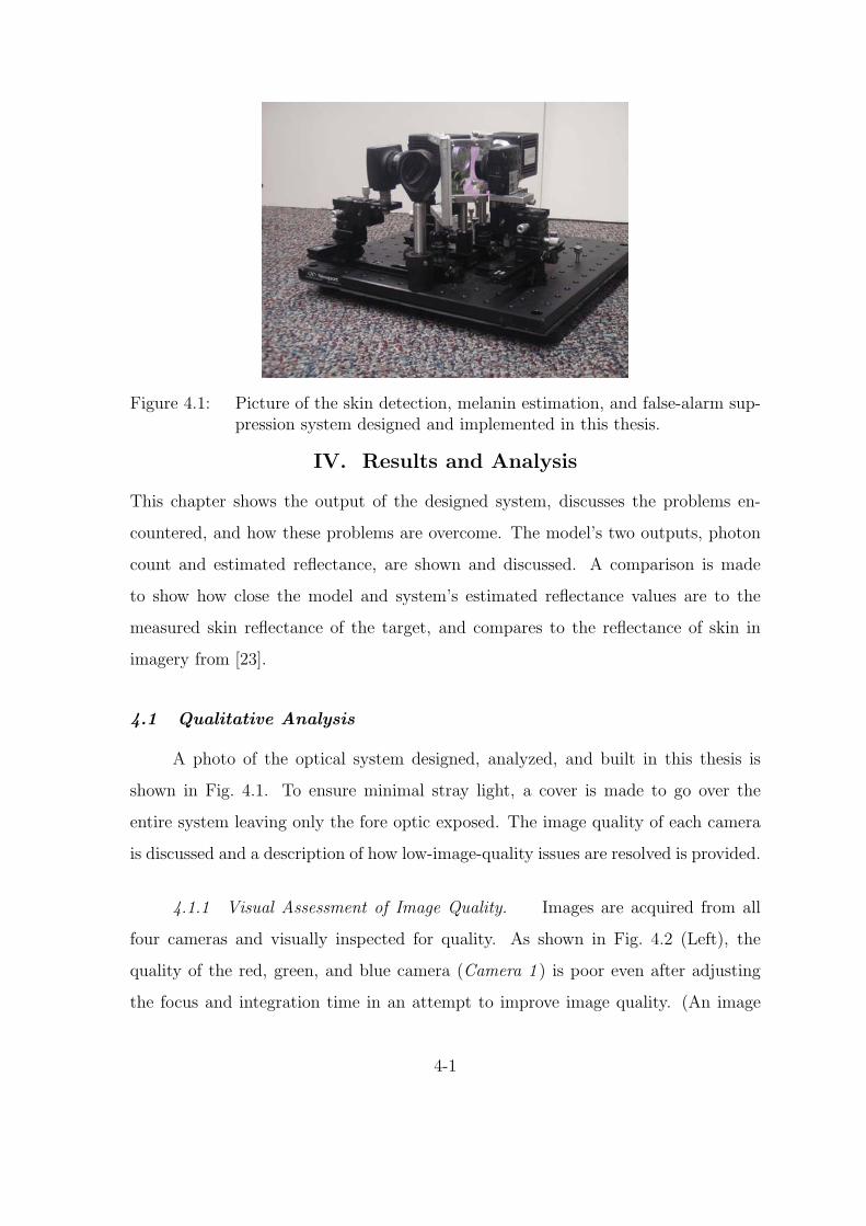
Figure 4.1: Picture of the skin detection, melanin estimation, and false-alarm sup-pression system designed and implemented in this thesis.

IV. Results and Analysis

This chapter shows the output of the designed system, discusses the problems en-

countered, and how these problems are overcome. The model’s two outputs, photon

count and estimated reflectance, are shown and discussed. A comparison is made

to show how close the model and system’s estimated reflectance values are to the

measured skin reflectance of the target, and compares to the reflectance of skin in

imagery from [23].

4.1 Qualitative Analysis

A photo of the optical system designed, analyzed, and built in this thesis is

shown in Fig. 4.1. To ensure minimal stray light, a cover is made to go over the

entire system leaving only the fore optic exposed. The image quality of each camera

is discussed and a description of how low-image-quality issues are resolved is provided.

4.1.1 Visual Assessment of Image Quality. Images are acquired from all

four cameras and visually inspected for quality. As shown in Fig. 4.2 (Left), the

quality of the red, green, and blue camera (Camera 1 ) is poor even after adjusting

the focus and integration time in an attempt to improve image quality. (An image

4-1

Figure 4.2: (Left) Image showing the highest visible quality image possible fromCamera 1 by adjusting the focus and integration time. (Right) Imageshowing the highest quality image possible from Camera 3 by adjustingthe focus and integration time. Note that focus decreases from left toright in the image.

from Camera 2, not shown, experiences the same effects.) To determine the source of

the poor image quality, the optical chain of Camera 1 is reassembled one component

at a time. The process of discovering the source of the problem and implementing a

solution is discussed in Section 4.1.2. Camera 3 and Camera 4 also show poor image

quality. Figure 4.2 (Right) shows the highest-quality image attained from Camera 3

by adjusting the focus and integration time. The poor quality is seen in comparing

the focus of the left and right sides of the image. (An image from Camera 4 is not

shown, but the same effects are seen.) Section 4.1.3 discusses the cause of the selective

focus problem and how it is resolved.

4.1.2 Addressing Image Quality Issues for Camera 1 and Camera 2. First,

the orientation of the achromatic doublet lens is checked, then an image is taken with

just the fore optic and the ThorLabs DCC1645C camera, the result of which is shown

in Fig. 4.3 (Left). As seen, the image comes to a crisp focus, demonstrating that the

image quality issue is not caused by these components. Next, Lens 2 is added to

the chain of Camera 1 and the image quality decreases, as seen in Fig. 4.3 (Right).

The effect seen (bright center, getting radially dimmer) is most likely vignetting.

4-2

Figure 4.3: (Left) Image acquired with the fore optic and ThorLabs DCC1645C(Camera 1 ). Note the image quality in terms of focus improved com-pared to Fig. 4.2. Issues with color seen are due to auto coloring andgaining aspects from the manufacturer’s software. (Right) Image ac-quired with the fore optic, second lens (Lens 1 ), and the ThorLabsDCC1645C Camera 1, where decreased image quality is seen.

Vignetting is defined as a clipping or truncation of the off-axis ray bundles by elements

distant from the aperture stop [9]. To solve this problem, an iris diaphragm is placed

directly in front of Lens 2 attached to Camera 1. The image shown in Fig 4.4 (Left)

has the diaphragm closed down to 8.3mm. The quality is greatly improved by this

addition, which indicates that vignetting is a issue. (The darkness around the top

of the image is due to a misalignment of the iris diaphragm relative to the center

of the lens. This issue is currently resolved and new images will be used in the

final thesis.) The last step is to insert the mirror into the optical chain, moving

Camera 1 to its original position. Figure 4.4 (Right) shows an image taken with all

of the elements in Camera 1’s optical chain. (The slight out of focus issue is caused

by the iris diaphragm not being centered on the lens, as seen in the image, but is

currently resolved.) Compared to the image seen in Fig. 4.3 (Right), there is a large

improvement in image quality due to the use of the iris diaphragm. Since the same

effects are seen in Camera 2, an iris diaphragm is added to correct for its poor image

quality. Fig. 4.5 (Left) and Fig. 4.5 (Right) demonstrate the image quality of Camera

1 and Camera 2 obtained by adding the iris diaphragms, respectively.

4-3

Figure 4.4: (Left) Image acquired with the fore optic, second lens (Lens 1 ), irisdiaphragm, and the ThorLabs DCC1645C (Camera 1 ). The iris di-aphragm is closed down to 8.3mm. (Right) Image acquired with thefore optic, second lens (Lens 1 ), iris diaphragm, Mirror 1, and theThorLabs DCC1645C (Camera 1 ). Some reduction in image quality isseen due to the iris diaphragm not being centered perfectly on the lens.

Table 4.1: Camera settings used to acquire the images shown in Fig. 4.5(Left,Right) and 4.6 (Left, Right).

Camera Integration Gain Filter DiaphragmTime (ms) Diameter (mm)

1 66.669 6 N/A 5.452 71.556 1 N/A 4.353 10.58 2 Semrock N/A

FF01-1060/13-254 18.77 2 Semrock N/A

NIR01-1570/3-25

4.1.3 Addressing Image Quality Issues for Camera 3 and Camera 4. The

effect seen in Camera 3 and Camera 4 is a result of the Scheimpflug principle [26].

This is where the lens plane is not parallel to the image plane and results in selective

focus. In the case of this specific system, the mirrors can contribute to this effect by

not being aligned to 45. To alleviate this issue, a compass is used to make sure each

mirror is as close to 45 as possible. The fore optic and cameras are adjusted to make

sure proper alignment is maintained and that they are not rotated in any direction.

4-4

Figure 4.5: (Left) Raw image from the ThorLabs DCC1645C used for NDGRIcalculation (Camera 1 ). (Right) Raw image from the ThorLabsDCC1545M used for melanin estimation (Camera 2 ).

Figure 4.6: (Left) Raw image from the Goodrich SU640KTSX-1.7RT used forskin detection (Camera 3 ) using the Semrock FF01-1060/13-25 filter.This configuration results in the light transmitting to (Camera 3 ) asshown in Fig 3.33 (blue curve). (Right) Raw image from the GoodrichSU640KTSX-1.7RT used for skin detection (Camera 4 ) using the Sem-rock NIR01-1570/3-25. This configuration results in the light transmit-ting to the (Camera 4 ) as shown in Fig 3.34 (green curve).

The images shown in Fig. 4.6 show the highest visual quality images available after

the mirrors, cameras, and lens positions are checked.

4-5

Table 4.2: Expected skin reflectance values generated by applying the transmissioncurves of Fig. 4.7 (Right) to the skin reflectance in Fig. 4.7 (Left) usedin comparing the model and the optical system.

Camera Configuration Reflectance Value

Camera 1 Green Channel 0.291Camera 1 Red Channel 0.427

Camera 2 0.544Camera 3 with Semrock FF01-1060/13-25 0.452Camera 4 with Semrock NIR01-1570/3-25 0.077

4.2 Quantitative Analysis

To collect data for the indoor scenario, the setup discussed in Section 3.5.1

is used. Images are acquired with a person, reflectance panels, and snow in the

scene. (The snow is common confuser due to its high scattering and water absorption

properties [23].) The use of three lamps is to attempt to achieve uniform illumination.

The camera parameters used to acquire the images are shown in Table 4.1. The

test setup and camera parameters apply to Fig. 4.5 and Fig. 4.6, which are the raw

images used in the analysis of the system. Here, the raw images are converted to

estimated reflectance using empirical line method (ELM). The reflectance estimated

by the model and the optical system developed in this thesis are compared to the

actual reflectance of human skin. The measured reflectance of the target used in this

comparison is shown in Fig. 4.7 (Left). Since the cameras are receiving broad spectral

bands of light, the true reflectance is not the reflectance at the center wavelength for

the given band. The actual reflectance value is a result of integrating across the bands

of the measured skin reflectance spectrally taking the system transmission from each

camera’s optical chain into consideration (Fig. 4.7) (Right). These computed values

are reported in Table 4.2.

4.2.1 Comparing Estimated Reflectance From the Physical System to Measured

Reflectance.

4-6

400 600 800 1000 1200 1400 16000

0.1

0.2

0.3

0.4

0.5

0.6

0.7

Wavelength (nm)

Ref

lect

ance

400 600 800 1000 1200 1400 16000

0.1

0.2

0.3

0.4

0.5

0.6

0.7

0.8

0.9

1

Wavelength (nm)

Tra

nsm

issi

on

Figure 4.7: (Left) Diffuse skin reflectance spectra obtained with a hand-held reflec-tometer, of the test subject used in validating the optical system andmodel. (Right) The transmissions used in the weighted average of theskin reflectance. The red and green curves represent the RGB camerachannel received spectra. The cyan curve represents Camera 2’s, blackrepresents Camera 3’s, and maroon represents Camera 4’s transmission

0.1 0.15 0.2 0.25 0.3 0.350

0.02

0.04

0.06

0.08

0.1

0.12

Reflectance

Pro

babi

lity

of R

efle

ctan

ce

0.2 0.25 0.3 0.35 0.4 0.45 0.50

0.02

0.04

0.06

0.08

0.1

0.12

Reflectance

Pro

babi

lity

of R

efle

ctan

ce

Figure 4.8: (Left) Distribution of 2184 neck pixels for the green channel of Cam-era 1. (Right) Distribution of 2184 neck pixels for the red channelof Camera 1. The red line shows where the expected diffuse skin re-flectance is located, per Table 4.2.

4.2.1.1 Camera 1. To determine how close the estimations are to the

expected values shown in Table 4.2, the pixels across the target’s neck are used. Fig-

ure 4.8 (Left) shows the distribution of the skin reflectance values for 2184 neck pixels

for the green channel of Camera 1. Similarly, Fig. 4.8 (Right) shows the distribution

of the skin reflectance values for 2184 neck pixels for red channel of Camera 1. The

red lines show the locations of the expected diffuse reflectance, per Table 4.2.

4-7

0

0.2

0.4

0.6

0.8

1

1.2

1.4

Figure 4.9: Estimated reflectance from Camera 2 using the raw data shown inFig. 4.5 (Right).

4.2.1.2 Camera 2. The estimated reflectance of Fig. 4.5 (Right) is

shown in Fig. 4.9. To see how close the estimations are to the expected values shown

in Table 4.2, a group of neck pixels is used. Figure 4.10 shows the distribution of

the skin reflectance values for 1960 neck pixels for Camera 2. The expected value is

right on the mode of the collected data. This shows the estimation for Camera 2 is

as expected.

4.2.1.3 Cameras 3 and 4. The estimated reflectance for Camera 3 and

Camera 4 are shown Fig. 4.11 (Left) and 4.11 (Right) respectively. Figure 4.12 (Left)

shows the distribution of the skin reflectance values for 2184 neck pixels for Camera

3. Figure 4.12 (Right) shows the distribution of the skin reflectance values for 2184

neck pixels for Camera 4. The red line shows where the expected diffuse reflectance

is located. The estimated reflectance values are near the expected reflectance values

for both Camera 3 and Camera 4.

4.2.1.4 Comparing Estimated Reflectance From the Physical System to a

Hyperspectral Imager. Using images collected from the HyperSpecTIR 3 (HST3),

4-8

0.35 0.4 0.45 0.5 0.55 0.6 0.65 0.70

0.02

0.04

0.06

0.08

0.1

0.12

0.14

Reflectance

Pro

babi

lity

of R

efle

ctan

ce

Figure 4.10: Distribution of 1960 neck pixels for Camera 2. The red line showswhere the expected diffuse skin reflectance is located, per Table 4.2.

0.2

0.4

0.6

0.8

1

1.2

0

0.5

1

1.5

2

Figure 4.11: (Left) Estimated reflectance from Camera 3 using the raw data shownin Fig. 4.6. (Left) Estimated reflectance from Camera 4 using the rawdata shown in Fig. 4.6 (Right).

the same estimated reflectance-based analysis is performed. The HST3 is an imaging

system with different noise characteristics, using two different detectors. Also, the

scene imaged has different targets and different illumination than the images taken

by the designed system. The expectation is that the distributions from these images

will be the same. A color image of the test scene is shown in Fig. 4.13 (Top). Since

the test images acquired for testing the skin detection system developed in this thesis

4-9

0.25 0.3 0.35 0.4 0.45 0.5 0.55 0.60

0.02

0.04

0.06

0.08

0.1

0.12

Reflectance

Pro

babi

lity

of R

efle

ctan

ce

0.03 0.04 0.05 0.06 0.07 0.08 0.09 0.1 0.11 0.120

0.02

0.04

0.06

0.08

0.1

0.12

0.14

Reflectance

Pro

babi

lity

of R

efle

ctan

ce

Figure 4.12: (Left) Distribution of 2184 neck pixels for Camera 3. (Right) Distri-bution of 2184 neck pixels for Camera 4. The red line shows wherethe expected diffuse skin reflectance is located, per Table 4.2.

Figure 4.13: (Top) Image acquired by HST3 used for comparison against the skindetection system data. (Bottom) Masked version of the image showingonly Type I/II skin used in the analysis.

only have a Type I/II skin target, a mask is used on the HST3 image so only the

same skin types are analyzed. The masked image is shown Fig. 4.13 (Bottom).

4-10

Since the system under test aggregates different portions of the spectrum than

the HST3 is capable of, we choose image bands in the HST3 imager as close to those

in the test system. The HST3 bands used for each portion of the spectrum are chosen

as:

• Red and green channels are converted to the XYZ colorspace defined by the

international commission on illumination, then to the RGB color space as ac-

complished in [23]

• To estimate melanin bands, the mean of the 18 HST3 bins with centers from

707.402nm to 907.557nm is used.

• The 1060nm Semrock bandpass filter uses the ∼8nm wide bin with a center at

1061.7nm.

• The 1570nm Semrock bandpass filter uses the ∼8nm wide bin with a center at

1570.83nm.

With the bands described above, the distributions shown in Fig. 4.14 - 4.16 are

created. The red line shows where the expected diffuse skin reflectance is located,

per Table 4.2. Figure 4.14 shows the distribution for the red channel (Left) and

green channel (Right) of the HST3 image. Figure 4.15 shows the distribution for the

melanin estimation channel of the HST3 image. Figure 4.16 shows the distribution for

the filtered 1060nm channel (Left) and filtered 1570nm channel (Right) of the HST3

image.

A visual inspection of both the HST3 and designed camera system’s histograms

indicates that they have similar shape. A more accurate comparison would be to

compute the similarity of both sets of distributions with a formal metric. This is

accomplished using the Bhattacharyya coefficient (BC). The BC is calculated by seg-

menting each distribution into an arbitrary number of bins based on their values and

then computing the coefficient as:

4-11

0.1 0.15 0.2 0.25 0.3 0.350

0.02

0.04

0.06

0.08

0.1

0.12

Reflectance

Pro

babi

lity

of R

efle

ctan

ce

0.15 0.2 0.25 0.3 0.35 0.4 0.45 0.50

0.02

0.04

0.06

0.08

0.1

0.12

Reflectance

Pro

babi

lity

of R

efle

ctan

ce

Figure 4.14: (Left) Distribution of the Type I/II skin pixels for the green channelof the HST3 image. (Right) Distribution of the Type I/II skin pixelsfor the red channel of the HST3 image. The red line shows where theexpected diffuse skin reflectance is located, per Table 4.2.

0.35 0.4 0.45 0.5 0.55 0.6 0.65 0.70

0.02

0.04

0.06

0.08

0.1

0.12

0.14

Reflectance

Pro

babi

lity

of R

efle

ctan

ce

Figure 4.15: (Left) Distribution of the Type I/II skin pixels for the melanin esti-mation channel of the HST3 image. The red line shows where theexpected diffuse skin reflectance is located, per Table 4.2.

BC =n∑

i=1

√pi · qi (4.1)

where pi and qi are the fraction of PMFs p and q that fall within the ith bin and n

is the number of bins. This results in a coefficient with a range of 0 (no overlap) to 1

(complete overlap) [28]. The BC computed between each pair of distributions of each

of the different bands is shown in Fig. 4.17. The BC indicates that the distributions

4-12

0.25 0.3 0.35 0.4 0.45 0.5 0.55 0.60

0.02

0.04

0.06

0.08

0.1

0.12

Reflectance

Pro

babi

lity

of R

efle

ctan

ce

0.03 0.04 0.05 0.06 0.07 0.08 0.09 0.1 0.11 0.120

0.02

0.04

0.06

0.08

0.1

0.12

0.14

Reflectance

Pro

babi

lity

of R

efle

ctan

ce

Figure 4.16: (Left) Distribution of the Type I/II skin pixels for the filtered 1060nmchannel of the HST3 image. (Right) Distribution of the Type I/II skinpixels for the filtered 1570nm channel of the HST3 image. The redline shows where the expected diffuse skin reflectance is located, perTable 4.2.

Red Green Mel 1060 15700

0.050.1

0.150.2

0.250.3

0.350.4

0.450.5

0.550.6

0.650.7

0.750.8

0.850.9

0.951

Bha

ttach

aryy

a C

oeffi

cien

t

Figure 4.17: The Bhattacharyya coefficient comparing each of the designed skindetection system distributions to the HST3 distributions. Red andgreen correspond to the color channels for Camera 1 ; Mel correspondsto Camera 2 ; 1060F and 1570F correspond to the use of the Semrockbandpass filters on Camera 3 and Camera 4.

are highly overlapping which indicates a good correspondence between the system

designed in thesis and the HST3 used for skin detection in [23] for similar targets.

4-13

4.2.1.5 Discussion. The histograms relative to the expected value of

the skin reflectance of the target at each camera are reasonable. In some cases, the

expected value corresponds well with the mode (Camera 2 and Camera 4 ). In other

cases, the expected value overestimates reflectance as indicated by the distributions

being skewed to the left (Camera 1 red and green channels and Camera 3 ). This

observation is consistent with the HST3 data. The spread of values in each of the

histograms is due to a number of factors including the effect of directional reflectance

and camera noise at each individual pixel. This is the case for all channels of the sys-

tem designed in the thesis as well as the HST3 imager. The bi-directional reflection

distribution function (BRDF) is an important aspect of the skin’s optical properties

and most likely has the largest effect on the spread of the estimations. This obser-

vation is supported by the high similarity between the distributions of the system

designed in this thesis compared to the HST3 as indicated by the high BC values.

The impact of not fully understanding the BRDF phenomena may result in the loss

of detections or an increase in false-alarms. A study needs to be accomplished on this

topic.

4.2.2 Comparing Modeled and Measured Reflectance.

4.2.2.1 Radiometric Model. To compare the model and measured

reflectance of human skin, the model is run with the same indoor setup (Fig. 3.25)

and camera specifications (Table 4.1) as the camera system. The radiometric model

calculates the number of electron forming photons that hit the focal plane array

and the estimated reflectance of a single target pixel using the process discussed in

Section 3.5.1.

First, the number of electron-generating photons for three targets are provided.

These targets include skin, a white Spectralonr panel, and a gray Spectralonr panel.

Figure 4.18 (Left) shows the theoretical number of electron generating photons for

each target per Eqn. (3.5). Figure 4.18 (Right) shows that the white Spectralonr

panel’s reflectance (red) is higher than the other targets and skin’s reflectance (green)

4-14

Green Red Mel 1060NF 1060F 1570NF 1570F LWPF10

0

101

102

103

104

105

106

107

108

Ele

ctro

n G

ener

atin

g P

hoto

ns

Wavelength Bands400 600 800 1000 1200 1400 16000

0.1

0.2

0.3

0.4

0.5

0.6

0.7

0.8

0.9

1

Wavelength (nm)

Ref

lect

ance

Figure 4.18: (Left) The number of electron-forming photons hitting the focal planearray of each camera with three different targets. The red × repre-sents the white Spectralonr panel, green ∗ represents skin, and blue represents the gray Spectralonr panel. The labels on the x axisof red and green correspond the color channels for Camera 1 ; Melcorresponds to Camera 2 ; 1060NF and 1570NF correspond to whatCamera 3 and Camera 4 see with only their respective mirrors reflect-ing and transmitting; 1060F and 1570F correspond to the use of theSemrock bandpass filters on Camera 3 and Camera 4. Lastly, LWPFcorresponds to the use of the Reynard corporation longwave pass filteron Camera 4. (Right) The measured reflectance of each target shownin the model. Red corresponds to the white panel, green correspondsto skin, and blue corresponds to the gray panel reflectance.

is higher than the gray panel’s (blue) out to 1370nm, where the gray panel’s becomes

larger than skin’s. Qualitatively, the photon counts agree with what is expected due

to the reflectance of each target. Furthermore, the system filter configurations that

have large pass bands show a higher photon count as expected.

To compare the radiometric model to the skin reflectance values in Table 4.2,

the photon count values need to be converted into reflectance using the empirical

line method. This conversion can be done because photon count relates directly to

the data numbers reported by the individual cameras. The Pwhite and Pgray values

discussed in Eqn. (3.6) are the red × and blue values shown in Fig. 4.18 (Left),

respectively.

The results of estimating the skin reflectance using the empirical line method

are shown in Fig. 4.19 as a red . Also shown on Fig. 4.19, as a blue ×, is the

4-15

Green Red Mel 1060NF 1060F 1570NF 1570F LWPF0

0.1

0.2

0.3

0.4

0.5

0.6

0.7

Ref

lect

ance

Figure 4.19: The estimated reflectance of skin found by using empirical line methodrepresented as a red . Actual skin reflectance is represented by a blue×. The labels on the x axis of red and green correspond the colorchannels for Camera 1 ; Mel corresponds to Camera 2 ; 1060NF and1570NF correspond to what Camera 3 and Camera 4 see with onlytheir respective mirrors reflecting and transmitting; 1060F and 1570Fcorrespond to the use of the Semrock bandpass filters on Camera 3and Camera 4. Lastly, LWPF corresponds to the use of the Reynardcorporation longwave pass filter on Camera 4.

actual measured reflectance value of skin used in the comparison [Fig. 4.18 (Right)].

Figure 4.20 shows the difference between the estimated and the actual reflectance of

the target.

4.2.2.2 Discussion. These results show theoretically that any filtering

choice for Camera 3 and Camera 4 provides the same result. With the values as

close as they are, the logical choice would be to use no filtering because the amount of

received energy is much higher, compensating for the relatively low solar illumination

in the NIR seen in Fig. 2.5. However as seen in Fig. 3.33 (Red) and Fig. 3.34 (Red),

the no-filter option integrates over a large band in which no study has been done to

4-16

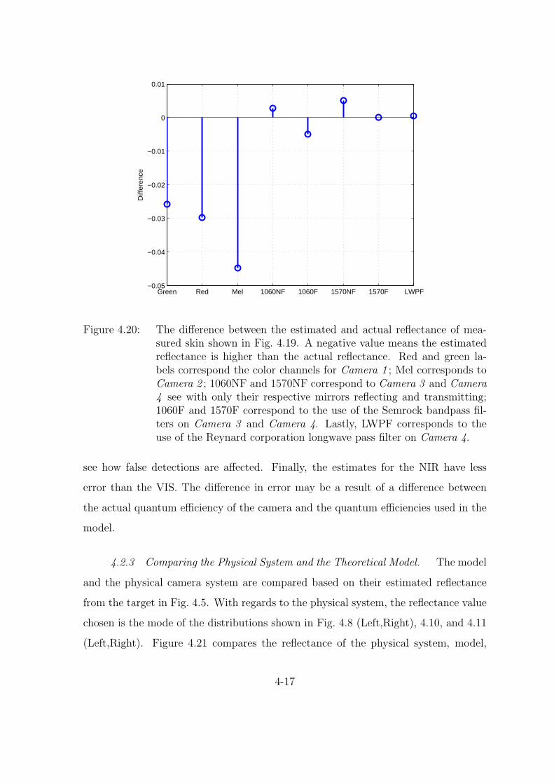
Green Red Mel 1060NF 1060F 1570NF 1570F LWPF−0.05

−0.04

−0.03

−0.02

−0.01

0

0.01

Diff

eren

ce

Figure 4.20: The difference between the estimated and actual reflectance of mea-sured skin shown in Fig. 4.19. A negative value means the estimatedreflectance is higher than the actual reflectance. Red and green la-bels correspond the color channels for Camera 1 ; Mel corresponds toCamera 2 ; 1060NF and 1570NF correspond to Camera 3 and Camera4 see with only their respective mirrors reflecting and transmitting;1060F and 1570F correspond to the use of the Semrock bandpass fil-ters on Camera 3 and Camera 4. Lastly, LWPF corresponds to theuse of the Reynard corporation longwave pass filter on Camera 4.

see how false detections are affected. Finally, the estimates for the NIR have less

error than the VIS. The difference in error may be a result of a difference between

the actual quantum efficiency of the camera and the quantum efficiencies used in the

model.

4.2.3 Comparing the Physical System and the Theoretical Model. The model

and the physical camera system are compared based on their estimated reflectance

from the target in Fig. 4.5. With regards to the physical system, the reflectance value

chosen is the mode of the distributions shown in Fig. 4.8 (Left,Right), 4.10, and 4.11

(Left,Right). Figure 4.21 compares the reflectance of the physical system, model,

4-17

and the actual reflectance values of the skin in Fig. 4.7 (Left). The red and green

show the widest variation. The system underestimates both channels, the red more

significantly. The model appears to overestimate, but only slightly. This is likely

because the model and the skin reflectance measurements do not contain a specular

component where as the measurements by the system do. The values for 1060F and

1570F are close in all three cases. A small difference still exists and this is most likely

do to BRDF properties that need to be studied. The reason that they are closer

than the other bands is due to the small bandwidth the Semrock filters transmit. As

shown in Fig. 4.19 the smaller bandwidths give better estimations of reflectance. The

estimated reflectance for the melanin band shows that the model estimates the values

higher than actual, but the physical system is very close to the actual value. The cause

for the model estimates to be further away than the system estimates is unclear. The

difference in error may be a result of the quality differences in the focal plane arrays,

which could indicate the Goodrich cameras (NIR) have less noise than the ThorLabs

cameras (VIS). Furthermore, this observation may support the statement that skin

is more specular in the VIS than the NIR due to the high absorption of the longer

wavelengths. Additional work is needed to better understand these issues.

4.3 Operational Analysis

The system’s operational ability to detect skin and discard false-alarms is dis-

cussed and shown in the subsequent sections.

4.3.1 Basic Skin Detection. The NDSI is calculated with the estimated

reflectance resulting in Fig. 4.22 (Left). By setting the upper and lower thresholds

for NDSI to 0.95 and 0.5 respectively, skin detection is accomplished and the snow as

well as other objects are falsely detected. The detection using just NDSI is shown in

Fig. 4.22 (Right).

4.3.2 False-Alarm Suppression. To perform the NDGRI calculation, the

reflectance of the red and green channels are estimated. The output of the NDGRI

4-18

Green Red Mel 1060F 1570F0

0.1

0.2

0.3

0.4

0.5

0.6

0.7

Ref

lect

ance

Wavelength Bands

Figure 4.21: Comparison of the model and physical system results. The red × rep-resents the physical system’s estimated reflectance, green ∗ representsthe model’s estimated reflectance, and blue represents the actualreflectance. Red and green correspond the color channels for Camera1 ; Mel corresponds to Camera 2 ; 1060F and 1570F correspond to theuse of the Semrock bandpass filters on Camera 3 and Camera 4.

−0.8

−0.6

−0.4

−0.2

0

0.2

0.4

0.6

0.8

1

Figure 4.22: (Left) NDSI calculated from the estimated reflectance of Camera 3 and4. (Right) Skin detection using NDSI only accomplished by settingbounded threshold between 0.5 and 0.95.

calculation is shown in Fig. 4.23 (Left). The noise resulting from the high digital gain

in Camera 1 is apparent in the NDGRI image, especially around the target’s hair and

the left reflectance panel (gray Spectralonr panel). The pixels that fall within the

threshold of -0.1 to -0.4 are shown in Fig. 4.23 (Right). Note that the snowball and

4-19

−0.5

−0.4

−0.3

−0.2

−0.1

0

0.1

0.2

0.3

Figure 4.23: (Left) NDGRI calculated from the estimated reflectance of the red andgreen channels of Camera 1. (Right) Pixels in the image meeting thebounded threshold between -0.1 and -0.4.

the other false-alarms shown in Fig. 4.22 (Right) are, for the most part, not included

in the detection shown in Fig. 4.23 (Right).

4.3.3 Rule-Based Skin Detection. Figures 4.22 (Right) and 4.23 (Right) are

multiplied together to make the final detection mask shown in Fig. 4.24. The false

detections in Fig. 4.24 occur for several reasons:

1. The target is not illuminated well enough and the noise dominated pixels result

in the calculated values erroneously appearing within the threshold region. This

issue is easily solved using a power threshold to ignore those pixels.

2. The cameras are not perfectly registered in both the x and y directions.

3. Camera 1 does not exactly have the same FOV as Cameras 3 and 4 due to the

pixel size difference. This means that Lens 2 may not be in the correct place.

4. Thresholds are not set correctly.

4.3.4 Melanin Estimation. The melanin estimation element has a significant

hardware issue. The drivers for the ThorLabs cameras do not allow for Camera 1 and

Camera 2 to run at the same time in MATLABr. As such, the melanin estimation

implementation is not shown in the thesis. Based on the reflectance estimation of

4-20

Figure 4.24: (Top) Image of the final detection after the bounded NDSI and NDGRIdetections are multiplied together. (Bottom) Color Image of scene tocompare skin detection against.

Camera 2 analyzed in Section 4.2.1.2 and the operational results provided for skin

detection, it is anticipated that the melanin estimation will work as expected and

described in [23].

4-21

4.4 Summary

The skin detection, melanin estimation, and false-alarm suppression system is

examined qualitatively, quantitatively, and operationally. Qualitatively, the image

quality issues are resolved so that the images can be in focus at any target distance.

Quantitatively, the model’s photon estimations agree with what is expected. The

estimated reflectance values from the camera system and the model compare favorably

to the skin’s measured reflectance. The distributions from the camera system are close

to the same distributions generated by the HST3 used in the original work specified

in [23]. This shows that two different imaging systems measuring under different

illuminations have the effect in their distribution. This gives reason to further pursue

topics such as BRDF. Operationally, skin detection and false-alarm suppression are

done as described in [23], and results indicate the system designed in this thesis meets

the intended use.

4-22

V. Conclusion

This chapter summarizes the accomplishments of this thesis and provides recommen-

dations for future work. Finally, the contributions of this thesis work are discussed.

5.1 Summary

In this thesis, two main topics are discussed: designing and building a monoc-

ular multi-spectral skin detection, melanin estimation, and false-alarm suppression

system [23] and designing a full radiometric model of that system. First, the oper-

ational scenarios for which this system is designed are low-altitude search missions,

where real-time skin detection is its main use. As such, a system that can capture

imagery at 1fps (with processing) and image at most 2in × 2in pixels from 710ft is

required [25]. With these specifications in mind, the cameras, lenses, mirrors, and

filters are selected. The camera selection is difficult due to a lack of visible cameras

with 25µm pixels. However, the problem is addressed using a second lens for both

visible cameras. The placement of each component makes it possible to use a single

fore optic so registration problems due to depth of field are not an issue. Having a

single fore optic makes it necessary for the incoming light to be divided appropri-

ately (as specified in [23]) to each camera. Custom dichroic mirrors are specified and

subsequently ordered to reflect and transmit the specific wavelengths to each camera

with very high efficiency. The spectrum received by the near-infrared cameras used

for skin detection are very broad so that different filtering bands can be experimented

with in the future.

5.2 Possibility of Future Work

There are several interesting area of future work based on this thesis. Future

work includes more advanced modeling, enhancements of the fore optic, enhancements

to the hardware, and additional analysis under a broad range of operating scenarios.

The results of a bi-directional reflectance function (BRDF) study on human

skin would be beneficial to better model the amount of energy that is incident on

5-1

the focal plane array resulting in a more accurate approximation of the what the

imager encounters. Since much of the detector theory is based on a diffuse reflectance

model [4,23] This might lead to a better understanding of the threshold values needed

or may result in new detector components to take this information into consideration.

Camera noise is another aspect that needs to be modeled. With the addition of

camera noise, the true response of the cameras can be modeled.

The physical system should be run through an optical design program so that

the highest quality images can be seen in all cameras. With such a program, a zoom

lens can be added to the system to enhance its operational use. For example, if a few

pixels are detected as skin, the camera can be zoomed into the area of interest for

more detailed view. Another issue at hand is understanding why the ThorLabs camera

drivers do not allow for both cameras to run at the same time inMATLABr. Further

work should address stability issues with the laptop frame-grabber cards required for

the Goodrich cameras. Moving to a laptop-based acquisition system increases system

flexibility for use in different operational environments.

Now that the system is built and running as expected, additional controlled

data collects need to be accomplished to determine how detecting and characterizing

skin is affected by illumination differences. As the model is modified with BRDF

and camera noise parameters, the model could be used to accomplish some of this

analysis. Additional analysis can include a study on how pixel size affects detection.

Finally, an in-depth study of the type of filters to use needs to be done to find what

filter combination gives the best detection and false-alarm performance.

5.3 Concluding Remarks

In this thesis, a complete optical system and model are developed to aid in

human skin detection. While skin detection is done presently, this system is the first

of its kind using VIS and NIR wavelengths to detect skin, suppress false-alarms, and

estimate melanin. These operations are done at frame rates of 10fps using engineering

software, but the cameras used can support up to 30fps. The search and rescue

5-2

community will benefit from this system by increasing the likelihood of image analysts

and ground teams finding lost persons. Not only search and rescue will benefit from

this. Special operations and manhunter missions can use the technology developed

here. Finally, the system developed provides a gateway to human measurements

and signatures intelligence (H-MASINT), and when combined with human detection

system such as that in [4], offers endless capability.

5-3

Bibliography

1. Brand, Jason and John S. Mason. “A comparative assessment of three approachesto pixel-level human skin-detection”. Proceedings of 15th International Confer-ence on Pattern Recognition, 1:1056–1059, Sep 2000.

2. Brandorff, Clemens. Rendering Human Skin. Technical report, Technishce Uni-versitat Wien, 2006.

3. Bretzner, Lars, Ivan Laptev, and Tony Lindeberg. “Hand Gesture Recognitionusing Multi-Scale Colour Features, Hierarchial Models and Particle Filtering”.Proceedings of the Fifth International Conference on Automatic Face and GestureRecognition, 405–410, May 2002.

4. Brooks, Adam Lee. Improved Multispectral Skin Detection and its Applicationto Search Space Reduction for Histograms of Oriented Gradients-based DismountDetection. Masters thesis, Air Force Institute of Technology, Wright-PattersonAFB, OH, 2010.

5. Clark, R. N., G. A. Swayze, R. Wise, K. E. Livo, T. M. Hoefen, R. F. Kokaly,and S. J. Sutley. “PinonPine ANP92-14A needle”. Webpage, 2007.

6. Daugman, John. “Face and Gesture Recognition: Overview”. IEEE Trans. onPattern Analysis and Machine Intelligence, 19(7):675–676, July 1997.

7. Dereniak, E. L. and G. D. Boreman. Infrared Detectors and Systems. John Wileyand Sons, 1996.

8. Eismann, M. T. Hyperspectral remote sensing. 2006. Classnotes.

9. Fischer, Robert E., Biljana Tadic-Galeb, and Paul R. Yoder. Optical SystemDesign. McGraw-Hill, Second edition, 2008.

10. Fleck, Margaret M. “Finding Naked People”. Proceedings of the 4th EuropeanConference on Computer Vision, 1065:593–602, 1996.

11. Gomez, Giovani. “On selecting colour components for skin detection”. Proceedingsof the International Conference on Pattern Recognition, 16(2):961–964, 2002.

12. Goodrich Sensors Unlimited, Princeton, NJ. Operation Manual: Compact InGaAsSnapshot Camera, 2007.

13. Hecht, Eugene. Optics. Pearson Education, 4th edition, 2002.

14. Hsu, Rein-Lein, Mohamed Abdel-Mottaleb, and Anil K. Jain. “Face detection incolor images”. IEEE International Conference on Image Processing (ICIP) 2001,1:1046–1049, October 2001.

15. Jacques, Steven L. “Skin Optics”. online:http://omlc.ogi.edu/news/jan98/skinoptics.html, Jan 1998.

BIB-1

16. Jengo, C.M. and J. LaVeigne. “Sensor performance comparison of HyperSpecTIRinstruments 1 and 2”. Proc. IEEE Aerospace Conference, 3:1805. March 2004.

17. Jones, Michael J. and James M. Rehg. “Statistical color Models with Applicationto Skin Detection”. International Journal of Computer Vision, 46(1), January2002.

18. Krishnaswamy, Aravind and Gladimir V.G. Baranoski. Eurographics, (3).

19. Lowel-Light Manufacturing. “Lowel Pro-light Instructions”, 2007.

20. Marschner, Stephen R., Stephen H. Westin, Eric P. Lafortune, Kenneth E. Tor-rance, and Donald P. Greenberg. “Image-Based BRDF Measurement IncludingHuman Skin”. Rendering Techniques, 131–144. 1999.

21. Matts, P.J., P.J. Dykes, and R. Marks. “The distribution of melanin in skindetermined in vivo”. British Journal of Dermatology, 156(4):620–628, Apr 2007.

22. Nicodemus, Fred E. “Directional reflectance and emissivity of an opaque surface”.Appl. Opt., 4(7):767–773, 1965.

23. Nunez, Abel S. A Physical Model of Human Skin And Its Application for Searchand Rescue. Ph.D. dissertation, Graduate School of Engineering, Air ForceInstitute of Technology (AETC), Wright-Patterson AFB OH, September 2009.AFIT/DEO/ENG/09-14.

24. Nunez, Abel S., Michael J. Mendenhall, Adam Brooks, and Richard K. Martin.“Hyperspectral Remote Sensing of Human Skin and its Level of Pigmentation”.IEEE Trans. Pattern Analysis and Machine Intelligence, 2009. Submitted.

25. Director of Operations, Mr. Chris Rowley. “Volunteer Image Analysts for Searchand Rescue (VIASAR)”.

26. Smith, Warren J. Modern Optical Engineering. McGraw-Hill, New York,, 4thedition, 2008.

27. Stevenson, B., R. O’Connor, W. Kendall, A. Stocker, W. Schaff, R. Holasek,D. Even, D. Alexa, J. Salvador, M. Eismann, R. Mack, P. Kee, S. Harris, B. Karch,and J. Kershenstein. “The Civil Air Patrol ARCHER Hyperspectral Sensor Sys-tem”. Airborne Intelligence, Surveillance, Reconnaissance (ISR) Systems andApplications II, 5787(1):17–28, 2005.

28. Thacker, N.A., F. J. Aherne, and P.I Rockett. “The Bhattacharyya Metric as anAbsolute Similarity Measure for Frequency Coded Data”. Kybernetika, 34(4):363–368, 1998.

29. The Infrared Information Analysis Center. The Infrared Handbook. 1993.

30. ThorLabs, Newton, NJ. Operation Manual: High-Resolution USB2.0 CMOS andCCD Cameras, 2009.

BIB-2

31. Weyrich, T., W. Matusik, H. Pfister, B. Bickel, C. Donner, C. Tu, J. McAndless,J. Lee, A. Ngan, H.W. Jensen, and M. Gross. “Analysis of Human Faces Using aMeasurement-Based Skin Reflectance Model”. volume 25, 1013–1024. 07 2006.

BIB-3

REPORT DOCUMENTATION PAGE Form ApprovedOMB No. 0704–0188

The public reporting burden for this collection of information is estimated to average 1 hour per response, including the time for reviewing instructions, searching existing data sources, gathering andmaintaining the data needed, and completing and reviewing the collection of information. Send comments regarding this burden estimate or any other aspect of this collection of information, includingsuggestions for reducing this burden to Department of Defense, Washington Headquarters Services, Directorate for Information Operations and Reports (0704–0188), 1215 Jefferson Davis Highway,Suite 1204, Arlington, VA 22202–4302. Respondents should be aware that notwithstanding any other provision of law, no person shall be subject to any penalty for failing to comply with a collectionof information if it does not display a currently valid OMB control number. PLEASE DO NOT RETURN YOUR FORM TO THE ABOVE ADDRESS.

1. REPORT DATE (DD–MM–YYYY) 2. REPORT TYPE 3. DATES COVERED (From — To)

4. TITLE AND SUBTITLE 5a. CONTRACT NUMBER

5b. GRANT NUMBER

5c. PROGRAM ELEMENT NUMBER

5d. PROJECT NUMBER

5e. TASK NUMBER

5f. WORK UNIT NUMBER

6. AUTHOR(S)

7. PERFORMING ORGANIZATION NAME(S) AND ADDRESS(ES) 8. PERFORMING ORGANIZATION REPORTNUMBER

9. SPONSORING / MONITORING AGENCY NAME(S) AND ADDRESS(ES) 10. SPONSOR/MONITOR’S ACRONYM(S)

11. SPONSOR/MONITOR’S REPORTNUMBER(S)

12. DISTRIBUTION / AVAILABILITY STATEMENT

13. SUPPLEMENTARY NOTES

14. ABSTRACT

15. SUBJECT TERMS

16. SECURITY CLASSIFICATION OF:

a. REPORT b. ABSTRACT c. THIS PAGE

17. LIMITATION OFABSTRACT

18. NUMBEROFPAGES

19a. NAME OF RESPONSIBLE PERSON

19b. TELEPHONE NUMBER (include area code)

Standard Form 298 (Rev. 8–98)Prescribed by ANSI Std. Z39.18

26–03–2010 Master’s Thesis Sept 2008 — Mar 2010

Design of a Monocular Multi-Spectral Skin Detection, MelaninEstimation, and False-Alarm Suppression System

09ENG287

Keith Robert Peskosky, Second Lieutenant, USAF

Air Force Institute of TechnologyGraduate School of Engineering and Management (AFIT/EN)2950 Hobson WayWPAFB OH 45433-7765

AFIT/GE/ENG/10-24

Dr. Brian Tsou711 Human Performance WingInformation Operations and Special Programs Branch

2210 8th Street, Bldg. 164, WPAFB, OH 45433937-785-8896; brian.tsou@wpafb.af.mil

AFRL/RHXB

Approval for public release; distribution is unlimited.

A real-time skin detection, false-alarm reduction, and melanin estimation system is designed targeting search and rescue (SAR) withapplication to special operations for manhunting and human measurement and signatures intelligence. A mathematical model of the systemis developed and used to determine how the physical system performs under illumination, target-to-sensor distance, and target-typescenarios. This aspect is important to the SAR community to gain an understanding of the deployability in different operatingenvironments. A multi-spectral approach is developed and consists of two short-wave infrared cameras and two visible cameras. Through anoptical chain of lenses, custom designed and fabricated dichroic mirrors, and filters, each camera receives the correct spectral information toperform skin detection, melanin estimation, and false-alarm suppression. To get accurate skin detections under several illuminationconditions, the signal processing is accomplished in reflectance space, which is estimated from known reflectance objects in the scene.Model-generated output of imaged skin, when converted to estimated reflectance, indicates a good correspondence with skin reflectance.Furthermore, measured and modeled estimates of skin reflectance indicate a good correspondence with skin reflectance.

Skin Detection, Melanin Estimation, False-Alarm Suppression, Multi-Spectral Imaging, Search and Rescue

U U U UU 116

Maj Michael J. Mendenhall

(937) 255–3636, ext 4614 Michael.Mendenhall@afit.edu