i

Acknowledgement

I gratefully acknowledge the efforts of Mr. Ogaba my project supervisor, in providing me

direction and guidance during the entire course of my project work. It has been pleasure and

honour to have been his student. I would like to recognize and appreciate my classmates for their

challenging criticism in my progress of the project and whose encouragement helped me greatly,

much appreciation too goes to staff of Electronics lab for their invaluable support.

ii

Dedication

This work is dedicated to my parents Richard and Mary Chebukto, their tireless efforts to keep

me in school and for helping me nurture my talent.

iii

Abstract

Air-core inductors are large-body low loss components that find frequent use in power

electronic converters and filter circuit design. The inductance value of such an inductor depend

on its geometry which can be varied by change in diameter of core, length of core, diameter of

wire and number of turns. It is often necessary to construct an inductor because specific

inductance values are difficult to find. In this project an investigation is carried out to determine

how inductance value changes with a single test parameter variation with all others being kept

constant. The main contributions of this project are a specific description of a practical approach

to determine inductance, where the inductor is connected in series with a resistor and RL circuit

properties are used to determine inductance value of a closely packed turn air core solenoid

inductors, the experimental results demonstrate the effect on inductance value of a single

parameter change at a time. The results suggest that a specific air core inductance value can be

realized by a wide variety of core inductor geometries.

iv

NOMENCLATURE

L inductance of a coil in henrys (H)

φ Number of flux lines contained in the loop (webers)

B Flux density (webers/ )

I Current in the loop

N Number of turns in the solenoid

Permeability of air (4 )

Length of solenoid

A cross sectional area of solenoid

Z Impedance of network

τ Time constant

D core diameter

d wire diameter

ρ Resistivity of wire copper wire 1.724× Ω/cm

v

Table of Contents

Acknowledgement ....................................................................................................................i

Dedication ............................................................................................................................. ii

Abstract.................................................................................................................................. iii

Nomenclature ......................................................................................................................... iv

1. CHAPTER ONE .................................................................................................................. 1

1.0 Introduction ...................................................................................................................... 1

1.1 Why air core .................................................................................................................... 1

1.2Chapters ahead .................................................................................................................. 1

2. CHAPTER TWO ................................................................................................................... 3

2.1 Faraday’s law .................................................................................................................. 3

2.2 Energy stored in an inductor............................................................................................. 4

2.3 Power losses in wound components ................................................................................. 5

2.3.1 Wire winding losses .............................................................................................. 6

2.4 loop quality factor ......................................................................................................... 6

2.5 Inductor operating frequencies ........................................................................................ 7

2.6 Complex impedances ...................................................................................................... 8

2.6.1 Argand Diagram .................................................................................................... 9

2.7 Series impedance of RL circuit ..................................................................................... 10

2.8 Inductor DC transient effects ........................................................................................ 10

2.9 Time constant .............................................................................................................. 12

2.10 Air core inductor specifications .................................................................................. 14

2.11 Applications of inductors ............................................................................................ 15

3. CHAPTER THREE ............................................................................................................... 17

3.0 design basis (Series RL-circuit) .................................................................................... 17

3.1 Investigating effect of inductance on parameter change ............................................... 18

3.1.0 Effect of varying the diameter of the core on inductance value ............................ 18

3.1.1 Effect of varying the number of turns on inductance value ................................... 18

3.1.2 Effect of varying length of core on inductance value ........................................... 19

3.1.3 Effect of varying the diameter of wire on the inductance value ............................ 19

3.1.4 effect of varying the number of layers of wire ................................................... 19

vi

3.2 Laboratory procedure to obtain inductance of solenoid .............................................. 19

3.2.0 Equipment ........................................................................................................ 19

3.2.1 Procedure ......................................................................................................... 20

3.3 results ......................................................................................................................... 21

4. CHAPTER FOUR ................................................................................................................. 24

4.0 Results analysis and comparison with theory ................................................................ 24

4.0.1 Graphs ................................................................................................................. 24

4.0.2 Discussion and comparison with theory ................................................................ 27

4.0.3 Number of turns of typical crossover inductors ..................................................... 30

5. CHAPTER FIVE ................................................................................................................. 31

5.0 Conclusion and further work ...................................................................................... 31

APPENDIX A ......................................................................................................................... 33

Inductor networks .............................................................................................................. 33

APPENDIX B ........................................................................................................................... 42

AWG/ metric conversion table ............................................................................................. 42

Reference ............................................................................................................................ 43

1

CHAPTER ONE

1.0 Introduction

An inductor is the magnetic force generated especially in a coiled wire that tries to oppose any

change in electric current that flows through it. This reaction of magnetic field that tries to keep

the current flow at a steady rate is called inductance. An air core inductor does not depend on a

ferromagnetic material to achieve the required inductance value. A non-ferromagnetic material

likes glass, wood or Bakelite can be used as the core in air core inductors.

1.1 Why air core?

Air core inductors are the only one that can achieve ideal inductive reactance behavior. They

have the highest stability, the tightest tolerance, a linear inductance under dynamic signal

condition, greater power handling and less distortion. They have relatively low d.c. resistance,

linear a.c. resistance, better and more linear quality factor at high frequency and linear phase

characteristics. They also have no magnetic core hysteretic distortion, no magnetic core

saturation distortion, no magnetic core non-linear inductance and no magnetic core phase

distortion. They also produce no harmonic frequency.

Without the use of high permeability core the challenges to encounter though it means the use

of many turns to achieve a given inductance value thus resulting in a bulky inductor, more turns

means high copper losses and low self resonance.

Inductors are used extensively in power conversion circuits. They are commonly used in input

and output in ac and dc systems. The concept of inductance is derived from Faraday’s Law

1.2 chapters ahead

Chapter two deals with the theory behind the behaviour of inductors and it highlights a literature

review of earlier developed relationship of inductance value on the physical parameters of the

inductors.

Chapter three emphasizes on the design theory and outlines an experimental procedure used to

determine inductance value of a closely packed solenoid, the effect of increasing the number of

layers is also outlined. Tabulated results and snapshots of oscilloscope images are included in

this chapter.

2

Chapter four contains discussion of results and comparison with theory. Graphs plotted using

MATLAB are also contained in this chapter, a relationship is of L with test parameters is

developed in this chapter.

Chapter five comprises the conclusion and future work to be done to improve on performance of

air core inductors

3

CHAPTER TWO

2.1 Faraday’s laws

This law forms the basis of determination of inductance value of wound components. The most

basic Self-inductance problem is the single turn loop inductor as shown in figure 2.0. Classical

Theory dictates that the self-inductance of this loop is determined by Faraday’s Law equation 2.1.0

W I

A=Area

S=perimeter

Figure 2.0

(2.1.0)

(2.1.1)

An induced electromotive force (voltage) in any circuit is always in a direction in opposition to

the current that produced it.

Consider a circuit with in which a current I is flowing. The current generates a magnetic field B

which gives rise magnetic flux ø linking the circuit. The flux is proportional to the current I.

From the law of magneto -statics we have

Ø = LI (2.1.2)

L is purely a geometric quantity that is, it is dependent on the shape of the circuit and the

number of turns.

If the current flowing in the circuit changes by a value in an interval then

magnetic flux linking the circuit changes by an amount in the same time interval.

According to Faraday’s law, an emf

4

(2.1.3)

is generated around the circuit. Also

(2.1.4)

Consider a solenoid of length l and cross-sectional area A and suppose the solenoid has N

turns, when a current I flows in the solenoid, a uniform axial field of magnitude

(2.1.5)

is generated in the core of the solenoid. The magnetic flux linking a single flux of the solenoid

is given by Ø = , thus the magnetic flux linking all flux of the solenoid is given by

Ø = (2.1.6)

The self- inductance can thus be written as

(2.1.6)

2.2 Energy stored in an inductor

When an inductor of inductance L is connected to a variable DC supply, and the supply is varied

to increase current flowing in the inductor from 0 to a final value I, as the current through the

inductor is increased an emf in equation 2.1.4 is generated which acts to oppose the increase in

current. The work done by the voltage source in order to establish current in the inductor is given

by

(2.2.1)

Where (2.2.2)

is the rate at which the voltage source performs the work. Integrating equation 2.2.1, we have

(2.2.3)

5

Giving (2.2.4)

The energy developed by the magnetic field is generated by the current flowing through the

inductor.

Writing the equation 2.2.4 as a function of N and l we obtain

(2.2.5)

Which reduces to

(2.2.6)

The volume of field –field solenoid is and the magnetic density of the solenoid is

(2.2.7)

The energy per unit volume in the solenoid is thus given by

(2.2.8)

When electric and magnetic field are both present then the total energy is given by

(2.2.9)

2.3 Power losses in wound components

Outlined here are the various causes of inefficiencies and techniques for minimizing them. Power

is lost in an air inductor through several different mechanisms:

Resistance of the windings – copper loss

Physical vibration and noise of the core and windings.

Electromagnetic radiation.

Dielectric loss in materials used to insulate the core and windings.

6

Only the copper loss operates even when the current in the winding is not changing. The other

losses all fall to zero with frequency.

2.3.2 Wire winding losses

Copper loss or winding loss is the term used to describe the energy dissipated by resistance in

the wire used to wind a coil. The behavior of an inductor at high frequencies is different from

that at low frequencies, at high frequencies the skin effect and come into play causing the

winding resistance to increase proportionally as and the inductance to decrease slightly with

increase in frequency of operation. The resistance of the winding is

(2.3.0)

Where l is the length of wire forming the turns round the solenoid. The resistivity of copper

wire at room temperature is 1.724× Ω/cm. The length of the wire comprising an N- turn

winding can be expressed as

l= N (MLT) (2.3.1)

Where MLT is the mean length per turn of the winding and is function of the core geometry.

Substituting (2.3.1) in (2.3.0) we have

(2.3.2)

2.4 Loop quality factor, Q

Loop quality factor is a measure of the losses in an inductive circuit. The resonant efficiency of a

circuit is expressed through the dimensionless quality factor Q. If the losses of the inductor are

large, Q is low. A perfect inductor has no losses; therefore, there is no dissipation of energy

within the inductor and Q is infinite.

Total energy loss in a loss inductor is calculated by modeling the

inductor as an equivalent lossless inductor in series with a resistor.

7

The quality factor is equal to the ratio of the inductive reactance to the resistive loss of the

inductor. Since inductive reactance is a frequency-dependent quantity, the frequency must be

specified when measuring quality factor. The formula for Q is written as

(2.4.1)

The Q of a resonant circuit is a measure of the ratio of the energy stored in it to the energy lost

during one cycle of operation. All practical inductors exhibit losses due to the resistance of the

wire or absorption by materials within the magnetic field surrounding it. Inductor losses are

modelled as a resistance, R, in series with a perfect or loss free inductance L as shown in fig

2.4.1

I

RLfigure 2.4.1

The value of R will be greater than that of the DC resistance of the wire due to skin effect. The

above formula suggests that the Q of any given inductor will increase indefinitely with

frequency. This is never the case because of an effect known as self resonance.

Practical values of Q range from around 10 for a high loss circuit through about 100 for a

reasonable one up to around 1000 with careful design and favourable condition.

2.5 Inductor operating frequencies

The behaviour of inductors at low frequencies is different from its behavior at high frequencies.

The construction of an inductor involves cramming a large amount of wire into a small volume,

and at radio frequencies, this means that the wavelength is likely to be comparable to the length

of the wire. The static magnetic conception of inductance works at low frequencies because the

8

length of the wire used to make the coil is much shorter than the wavelength. This means that a

wave entering the coil at one terminal will emerge from the other terminal with almost exactly

the same phase. Thus an instantaneous view of the magnetic field surrounding the coil will be

almost identical to the field produced by a direct current; in which case, the energy stored (LI²/2)

will be the same as in the DC case and the inductance can be calculated accordingly. From an

electrical point of view therefore, a coil operating at low frequencies looks like a lumped

inductance in series with the DC resistance of the wire.

2.6 complex impedances

Impedance of any given network is given by equation 2.6.1

V = IZ (2.6.1)

If the network consists of a single resistor, Z = R. For networks containing an inductor as shown

in fig 2.6.1

figure 2.6.1

The voltage across an inductor is given by:

V = L ( dI /dt ) (2.6.1)

Also

V = IZL (2.6.2)

Setting 2.61 and 2.6.2 equal:

L ( dI /dt ) = IZL (2.6.3)

dI /I = (ZL /L) dt (2.6.4)

n I = ( ZLt /L ) + n Io (2.6.5)

9

t/LZo

LeII (2.6.6)

Now if ZL is a real positive number, the current must increase exponentially. If ZL is a real

negative number, it must decrease exponentially toward zero. If ZL is zero, the voltage is

identically zero. To get a useful relationship let ZL vary with time. But time varying impedance

is not a useful concept for a simple inductor. A viable solution is to move out of the domain of

real numbers and explore the possibility of letting ZL be imaginary or possibly complex.

Ltj

otj

o ZeIeIdt

dL

(2.6.7)

LIoj ej t

= Ioej t

ZL (2.6.8)

j L = ZL (2.6.9)

Since the impedance depends on the frequency. Thus different harmonics of a periodic waveform

will encounter different impedances.

It should be noted that as frequency increases, the impedance of an inductor increases

2.6.1 Argand Diagram

Used to express the relationship between current and voltage across the inductor

Rej

= Rcos + jRsin

= X + jYR

Fig 2.6.2

Z = j L plots as:

Another way to express this Z is as Lej /2

. I = Ioej t

plots as:

10

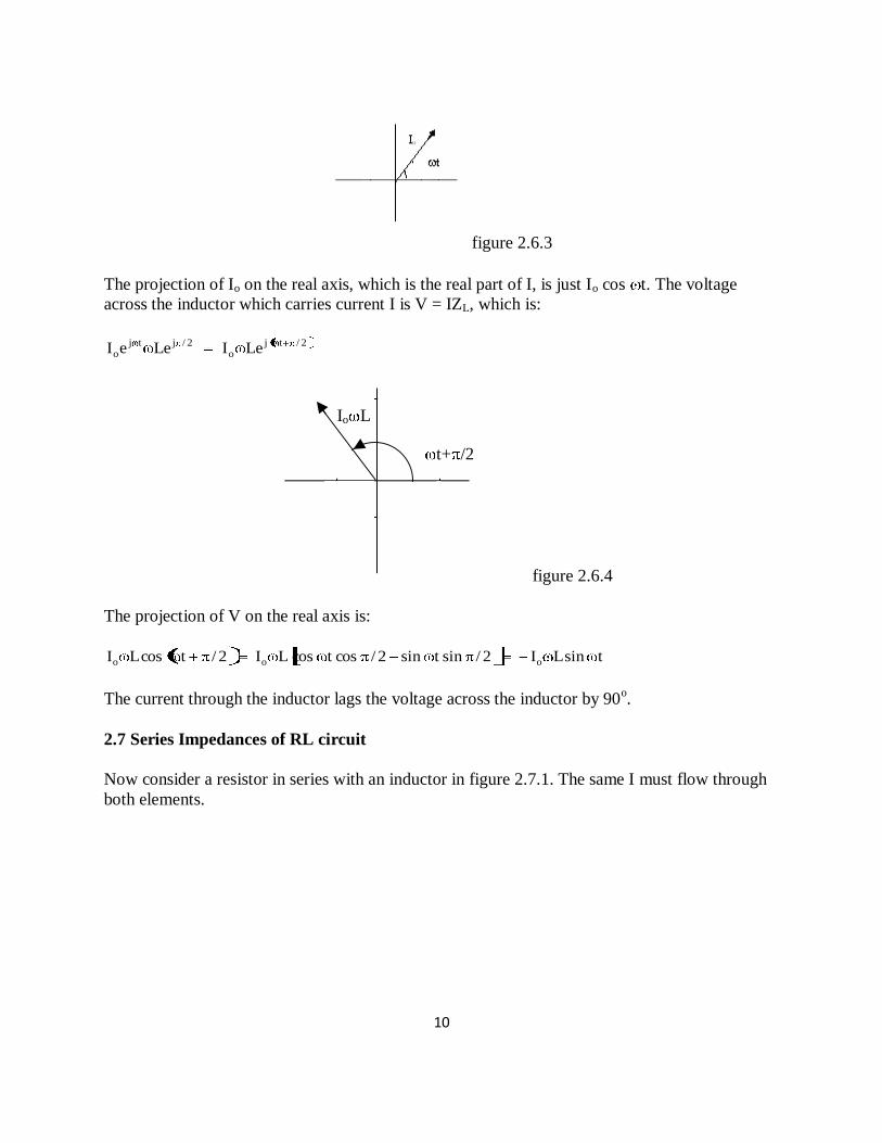
figure 2.6.3

The projection of Io on the real axis, which is the real part of I, is just Io cos t. The voltage

across the inductor which carries current I is V = IZL, which is:

2/tjo

2/jtjo LeILeeI

Io L

t+ /2

figure 2.6.4

The projection of V on the real axis is:

tsinLI2/sintsin2/costcosLI2/tcosLI ooo

The current through the inductor lags the voltage across the inductor by 90o.

2.7 Series Impedances of RL circuit

Now consider a resistor in series with an inductor in figure 2.7.1. The same I must flow through

both elements.

11

figure 2.7.1

Vb = IZL = Ij L (2.7..1)

Va = Vb + IR = Ij L + IR = I(R + j L) (2.7.2)

Va = IZL,R = Ioej t 222 LR e

j , (2.7.3)

Where tan = L/R

ZL,R = 222 LR ej

(2.7.4)

With complex impedances, all the rules for series impedance, parallel impedance, and voltage

dividers will be the same as they are with resistors, since the derivations are depended only on

the equation V = IZ which is comparable to V = IR in the case of resistors.

2.8 Inductor D.C transient effects

Consider an inductor in series with a resistor and a source of a constant EMF. At time t = 0, the

switch is closed, and current will suddenly attempt to flow. The sudden change in current will

cause a counter EMF to be self-induced in the coil to oppose the change in current. This counter

EMF will initially be exactly equal to the applied EMF so that no current will initially flow. As

the current starts to flow, its rate of increase will decrease, and the counter EMF will likewise

decrease, allowing more current to flow. The current will increase exponentially until its

maximum value is reached, as determined by the series resistance in the circuit.

12

Figure 2.8.1 Charging Inductor

After a fairly long period of time has passed, the initial transient effects will have died down and

a steady dc current will be flowing through the inductor. This dc current will create a constant

magnetic field within the inductor. Any attempt to change quickly this constant field will be

opposed by the inductor.

Assume that a coil or inductor has a constant current flowing through it and all initial transient

effects have decayed. At time t = 0, the coil will be instantly short circuited across a resistance.

The field will slowly collapse, eventually causing a current to flow until there is no more

magnetic field and, correspondingly, no current is flowing. This decrease in current is

exponential.

Figure 2.8.2 Discharging Inductor

2.9 Time Constant (τ)

It is a measure of time required for certain changes in voltages and currents in RC and RL

circuits. Generally, when the elapsed time exceeds five time constants (5τ) after switching has

13

occurred, the currents and voltages have reached their final value, which is also called steady-

state response.

The time constant of an RL circuit is the equivalent inductance divided by the Thévenin

resistance as viewed from the terminals of the equivalent inductor.

τ = L/ R

Current in an RL circuit has the same form as voltage in an RC circuit: they both rise to their

final value exponentially according to

1-

The expression for the current build-up across the Inductor is given by

(t)= (1- ) t ≥ 0 (2.8.1)

Where, V is the applied source voltage to the circuit for t ≥ 0. The response curve is

increasing and is shown in Figure 2.8.3

Fig. 2.8.3 Current build up across Inductor in a Series RL circuit.(Time axis is

normalized by τ)

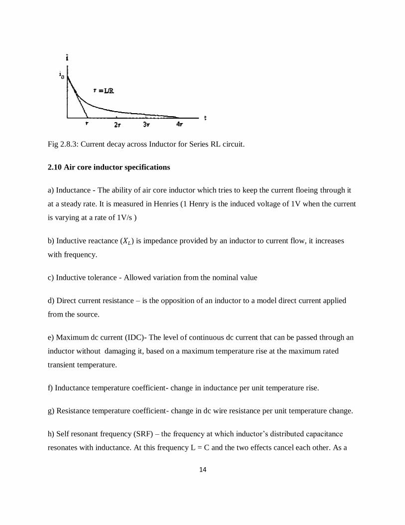
The expression for the current decay across the Inductor is given by:

(t)= t ≥ 0 (2.8.2)

Where, is the initial current stored in the inductor at t = 0 and L/R = τ is time constant.

The response curve is a decaying exponential and is shown in Figure 2.8.3

14

Fig 2.8.3: Current decay across Inductor for Series RL circuit.

2.10 Air core inductor specifications

a) Inductance - The ability of air core inductor which tries to keep the current floeing through it

at a steady rate. It is measured in Henries (1 Henry is the induced voltage of 1V when the current

is varying at a rate of 1V/s )

b) Inductive reactance ( ) is impedance provided by an inductor to current flow, it increases

with frequency.

c) Inductive tolerance - Allowed variation from the nominal value

d) Direct current resistance – is the opposition of an inductor to a model direct current applied

from the source.

e) Maximum dc current (IDC)- The level of continuous dc current that can be passed through an

inductor without damaging it, based on a maximum temperature rise at the maximum rated

transient temperature.

f) Inductance temperature coefficient- change in inductance per unit temperature rise.

g) Resistance temperature coefficient- change in dc wire resistance per unit temperature change.

h) Self resonant frequency (SRF) – the frequency at which inductor’s distributed capacitance

resonates with inductance. At this frequency L = C and the two effects cancel each other. As a

15

consequence at SRF , the inductor acts as a purely resistive high-impedance element. Also at this

frequency Q= 0. Distributed capacitance is caused by the turns of core layered on top of each

other and around the core.

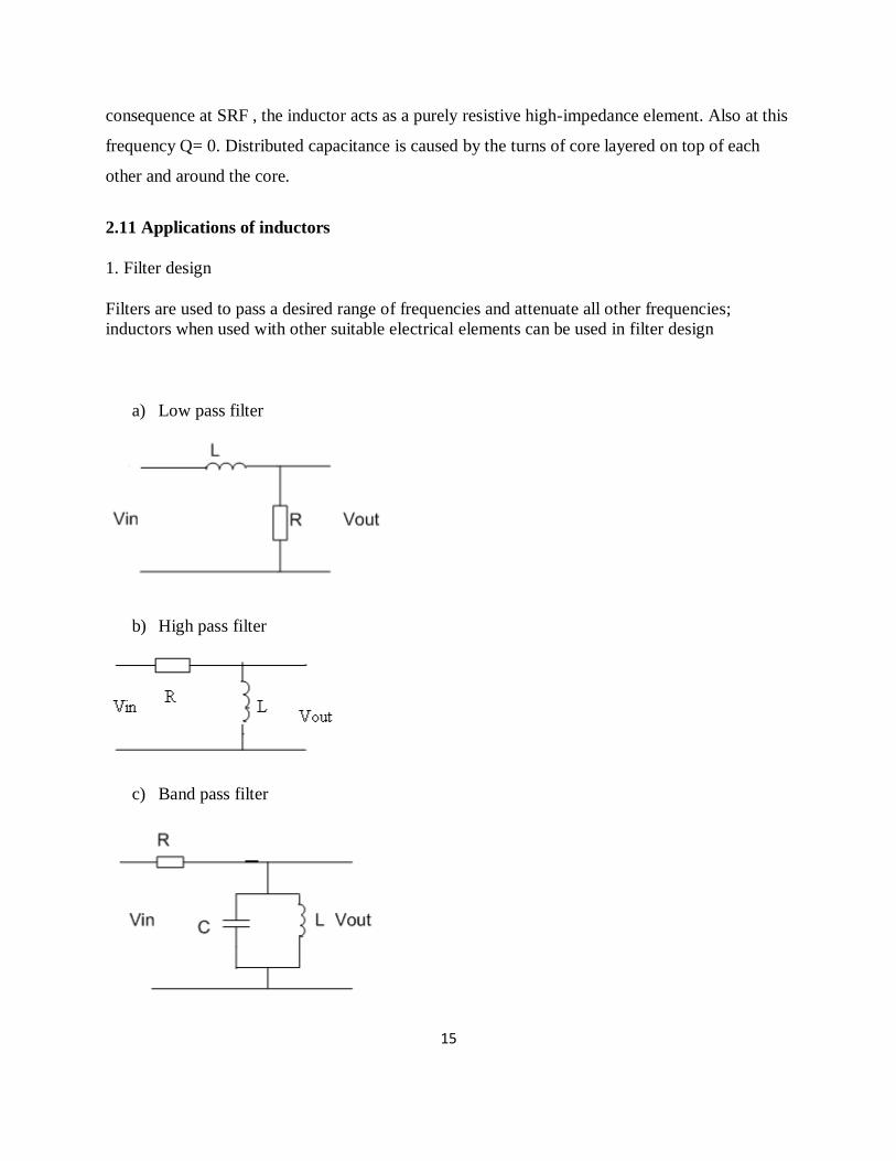
2.11 Applications of inductors

1. Filter design

Filters are used to pass a desired range of frequencies and attenuate all other frequencies;

inductors when used with other suitable electrical elements can be used in filter design

a) Low pass filter

b) High pass filter

c) Band pass filter

16

2. Regulator design (Buck, boost and buck and boost regulators)

3 Op amp oscillator design

4 Colpits oscillator and Hartley oscillators

5. Radio circuits – SW receiver, RF oscillator/ transmitter

17

CHAPTER THREE

3.0 design basis (series RL-circuit)

figure 3.0

The relationship of , and in a RL circuit is represented by vector diagram 3.1

VLVs

VR Io A

B

ø

figure 3.1

Voltage drops are shown in voltage triangle OAB in figure 3.1. Vector OA represents ohmic drop

and AB represents inductive . The applied voltage is the sum of the two i.e

= = = ,

I=

18

tan, ø = = =

The resistance was chosen to have a value almost equal to the reactance of the inductor so that

the ~ , with this consideration then I=

The inductance value was calculated by we use the equation 3.0.1 obtained from; =I. = I. 2

fL. Where f is set from the signal generator.

L= /2 fI (3.0.1)

3.1 Investigating effect of inductance on parameter change

The diameter of wires were measured using a micrometer screw gauge was converted to a

corresponding SWG value using table B in appendix.

3.1.0 Effect of varying the diameter of the core on inductance

The diameters of 6 separate wooden cores were measured by vernier callipers and were found to

be 10.8mm, 12.7mm, 16.4mm, 20.6mm, 29.9mm and 44.4mm.

With d, N and l kept constant the results obtained from the measurements were recorded in table

3.3.4. L was calculated from the figures in the table.

3.1.1 Effect of varying the number of turns on inductance value

With D and d kept constant 77,124 and 160 turns were made on the circular cores. Turns of

237,284 and 361 were made by connecting suitable solenoids in series. Results obtained and the

inductances value calculated were recorded in table 3.3.1

19

3.1.2 Effect of varying the length of core on inductance value

Cores of lengths 54mm, 92mm, 116mm, 146mm, 170mm, 208mm and 262mm were used to

investigate this effect. D, N and d were kept constant. The calculated inductance as a result of

varying core length was recorded in table 3.3.2

3.1.3 Effect of varying the diameter of wire on the inductance value

Wires of diameters 0.33, 0.46, 0.49 and 0.69 were wound on core of diameter 6.23mm and

length 28mm. The turns were tightly packed; inductance value was calculated and recorded in

table 3.3.3

3.1.4 Effect of varying the number of layers of wire

Solenoids of lengths and layers tabulated in 3.3.5 were tested and their inductance value

calculated. Their inductance value was calculated and recorded.

3.2 Laboratory procedure to obtain inductance of a solenoid

The objective of this laboratory procedure was to investigate the inductance concept and observe

the voltage drop across the inductor.

3.2.0 Equipment:

• Digital Multi-meter

• Signal generator

• Oscilloscope

• Resistors

• Solenoids of different parameters

20

3.2.1 Procedure

1. The internal resistance of the coil (r) was measured using a multi-meter and its value

recorded. The signal generator consisted of a variable emf source ( ) and variable frequency

source.

2. The apparatus were connected as indicated in fig 3.2.1 the negative side of the function

generator was grounded. Channel 1 of the oscilloscope connected across the source and channel

2 connected across the R.

fig 3.2.1

3. Resistors R were chosen with a value close to the reactance of the inductor, this was achieved

by choosing a resistor which gave a voltage drop with amplitude approximately half that of input

voltage. Where need be resistors were connected in parallel or series to give the desired value of

resistance.

4. The current in the circuit was calculated by, I=

5. The procedure was repeated for all the coils and their values recorded in table’s 3.3.1-3.3.5

6. the inductance of each test coil was calculated by equation 3.0.1

21

3.3 Results

Table 3.3.1 showing how inductance varies with the number of turns

N R(Ω)

77 6 100 68.34 73 2.5 27.3 4.3

124 6 200 145.7 137 6.67 21.84 9.98

160 6 200 144.3 138.5 10 14.43 15.3

201 6 200 143 139.7 16.7 8.6 25.87

237 6 200 141.8 141 23.3 6.1 36.8

284 6 200 140.23 142.6 30 4.67 46

361 6 200 139.4 143.4 50 2.8 81.5

Table 3.3.2 showing how inductance varies with length of core

R(Ω)

54 6 100 68.34 73 2.5 27.3 4.3

92 6 200 145.7 137 6.67 21.84 9.98

116 6 200 144.3 138.5 10 14.43 15.3

146 6 200 143 139.7 16.7 8.6 25.87

170 6 200 141.8 141 23.3 6.1 36.8

208 6 200 140.23 142.6 30 4.67 46

262 6 200 139.4 143.4 50 2.8 81.5

Table 3.3.3 showing effect of varying diameter of wire on inductance

SWG R(Ω)

0.33 29 150 105.1 107 10 10.5 16.2

0.46 26 150 105.9 106.2 6.7 15.9 10.6

049 25 150 106.9 105.4 5 7.8 7.8

0.69 22 150 107.2 104.9 3.3 5 5

22

Table 3.3.4 showing variation of inductance value with core diameter change

N R(Ω)

31 10.8 150 114 98 40 2.85 5

31 12.7 150 112 99.8 40 2.8 6.6

31 16.4 150 109 103 60 1.82 9

31 20.6 150 107 105 100 1.07 15.4

31 29.9 150 104 108 165 0.69 27.2

31 44.4 150 101 110 300 0.34 52.6

Table 3.3.5 Effect of increasing the number of layers on inductance

layers N

1 384 206 170 54 113 92.79

2 383 90 215 115 98 227.85

3 383 61 270 175 95 357.7

4 383 46 320 230 87 513.32

23

Figure 3.3.6 the bigger magnitude waveform indicates voltage from the supply and the smaller

amplitude indicates voltage across the resistor, the vector difference indicates the voltage across

the inductor.

Fig 3.3.6 showing and snapshot taken in an oscilloscope.

24

CHAPTER FOUR

4.0 Results analysis and comparison with theory

To aid analysis; graphs showing variation of inductance with number of turns, variation of

inductance with diameter of wire, variation of inductance with diameter of core and variation of

inductance with length of core were plotted on different scales using MATLAB. A line of best fit

was plotted for each graph, this is done to take care of experimental errors in the lab and to cater

for truncation in calculus brought about by calculation of the inductance value, other errors

which may have brought about imperfect curves were the reading errors of measuring

instruments used (micrometer screw gauge, vernier calipers and ruler). The graphs plotted are

labelled 4.0.1-5

4.0.1 Graphs

figure 4.0.1

25

Figure 4.0.2

Figure 4.0.3

26

Figure 4.0.4

figure 4.0.5

27

With curve of best fit tool in MATLAB the equation for curve of best fit in each graphs are

4.0.2 Discussion and comparison with theory.

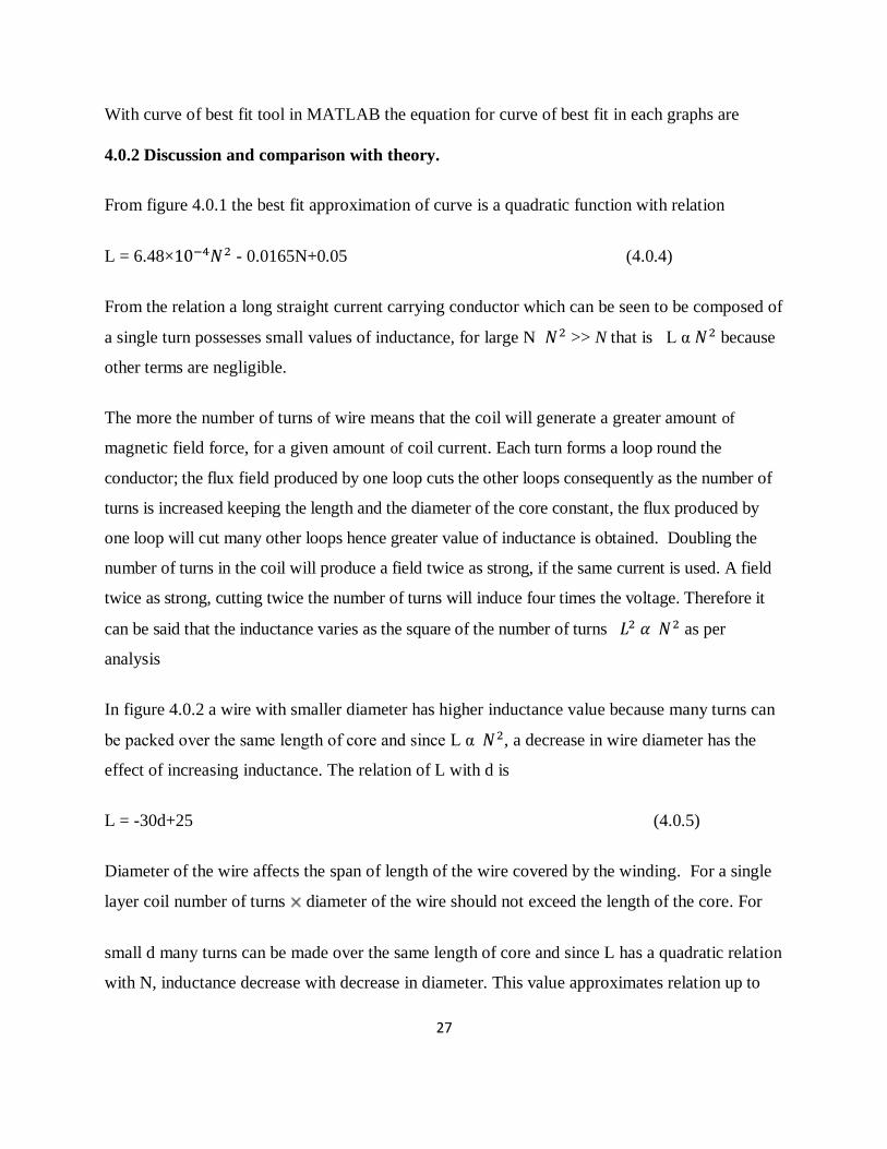
From figure 4.0.1 the best fit approximation of curve is a quadratic function with relation

L = 6.48× - 0.0165N+0.05 (4.0.4)

From the relation a long straight current carrying conductor which can be seen to be composed of

a single turn possesses small values of inductance, for large N >> N that is L α because

other terms are negligible.

The more the number of turns of wire means that the coil will generate a greater amount of

magnetic field force, for a given amount of coil current. Each turn forms a loop round the

conductor; the flux field produced by one loop cuts the other loops consequently as the number of

turns is increased keeping the length and the diameter of the core constant, the flux produced by

one loop will cut many other loops hence greater value of inductance is obtained. Doubling the

number of turns in the coil will produce a field twice as strong, if the same current is used. A field

twice as strong, cutting twice the number of turns will induce four times the voltage. Therefore it

can be said that the inductance varies as the square of the number of turns as per

analysis

In figure 4.0.2 a wire with smaller diameter has higher inductance value because many turns can

be packed over the same length of core and since L α , a decrease in wire diameter has the

effect of increasing inductance. The relation of L with d is

L = -30d+25 (4.0.5)

Diameter of the wire affects the span of length of the wire covered by the winding. For a single

layer coil number of turns diameter of the wire should not exceed the length of the core. For

small d many turns can be made over the same length of core and since L has a quadratic relation

with N, inductance decrease with decrease in diameter. This value approximates relation up to

28

d=0.833 mm (SWG=21). To expand this relation to include bigger diameters, a variety of large

size wire diameters need to be tested.

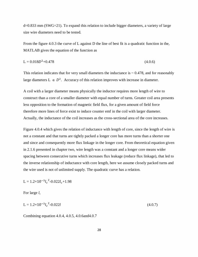
From the figure 4.0.3 the curve of L against D the line of best fit is a quadratic function in the,

MATLAB gives the equation of the function as

L = 0.018 +0.478 (4.0.6)

This relation indicates that for very small diameters the inductance is ~ 0.478, and for reasonably

large diameters L α . Accuracy of this relation improves with increase in diameter.

A coil with a larger diameter means physically the inductor requires more length of wire to

construct than a core of a smaller diameter with equal number of turns. Greater coil area presents

less opposition to the formation of magnetic field flux, for a given amount of field force

therefore more lines of force exist to induce counter emf in the coil with larger diameter.

Actually, the inductance of the coil increases as the cross-sectional area of the core increases.

Figure 4.0.4 which gives the relation of inductance with length of core, since the length of wire is

not a constant and that turns are tightly packed a longer core has more turns than a shorter one

and since and consequently more flux linkage in the longer core. From theoretical equation given

in 2.1.6 presented in chapter two, wire length was a constant and a longer core means wider

spacing between consecutive turns which increases flux leakage (reduce flux linkage), that led to

the inverse relationship of inductance with core length, here we assume closely packed turns and

the wire used is not of unlimited supply. The quadratic curve has a relation.

L = 1.2× -0.022 +1.98

For large l,

L = 1.2× -0.022l (4.0.7)

Combining equation 4.0.4, 4.0.5, 4.0.6and4.0.7

29

We obtain

= (6.48× - 0.0165N+1.9731)( -30d+25)( 0.018 +0.478)( 1.2× -0.022 )

L ~

This relates the inductance with test parameters for single layer air core coil inductor.

The inductance value can be increased by a great factor by winding the turns in layers as shown

in table 3.3.5

Where L is in µH.

According to theory there are developed formulas which give inductors of air coil inductors, for

single layer Wheeler’s formula shown in equation 4.0.7 best approximates the inductance value

where a=radius of solenoid

For multilayer the formula does not hold because the incidence of turn to turn, turn to layer

magnetic coupling is increased

The formula which is used is

L=

Where d = depth of winding (outer diameter- inner diameter)

r = mean radius of coil

l = length of coil in inches.

30

The formulas does not put into consideration the wire gauge the reason could be the aspect wire

gauge and length of core are related by d = once the length of core and N are considered then

by intuition the wire gauge effect comes into play.

4.0.3 Number of turns for typical crossover inductors

Typical crossover used inductors are valued at 2.82 and = 0.42

This value is high to be achieved by single layer air core inductor therefore we use multilayer air

core.

Possible multi-layer core to achieve the above results is obtained by extrapolating results of

figure 4.0.5.

The number of turns required to obtain an inductance value of 0.42mH = 420 H is a 3 layer

N=383, core length is 70mm, d=0.46mm and D = 13mm

The number of turns required to obtain an inductance value of 2.82 = 2.82 × is a 6

layer=383,core length is 70mm, d=0.46mm D = 13mm.

31

CHAPTER FIVE

5.0 Conclusion and further work

A specific air core inductance value can be obtained by changing the various geometric

parameters of the inductor. Generally the inductance value of air core inductors is low but

because of their linear behavior and lack of harmonics they find wide use in high frequency

requirement applications. An ideal inductor described as one with no internal resistance and does

not dissipate or radiate energy is not achievable in practice because inductors are made of wires.

Inductors do not behave like resistors which simply oppose current flow inductors oppose

changes in current through them; they drop a voltage directly proportional to the rate of change

of current, this induced voltage is always of such a polarity as to try to maintain current at its

present value. The voltage drop across the inductor is a reaction to change in current across it.

Because instantaneous power is the product of the instantaneous voltage and the instantaneous

current the power equals zero whenever the instantaneous current or voltage is zero. Whenever

the instantaneous current and voltage are both positive, the power is positive. In inductor because

the current and voltage waves are 90o out of phase, there are times when one is positive while the

other is negative, resulting in equally frequent occurrences of negative instantaneous power.

Negative power means that the inductor is releasing power back to the circuit, while a positive

power means that it is absorbing power from the circuit. Since the positive and negative power

cycles are equal in magnitude and duration over time, the inductor releases just as much power

back to the circuit as it absorbs over the span of a complete cycle. The inductive opposition to

alternating current is similar to resistance, but different in that it always results in a phase shift

between current and voltage, and it dissipates zero power.

If the frequency equals zero, then so does the impedance - a frequency of zero means DC, so

inductors have virtually no resistance to DC current flow but does not allow whole of source

current to flow through it because it possesses internal resistance. And as the frequency goes up,

so does the impedance. This is opposite behaviour compared to capacitance. Future work in the

air core inductor field includes:

32

To develop computer software that gives the inductance when given inductor

specification.

Design a RCL bridge that measures inductance value

To investigate the dimensions which give optimum inductance per unit area.

Investigate on possibility of developing an inductor which comes as an integrated chip

33

APPENDIX A

1 Inductor networks

Inductors in series

Inductors in parallel

a) Inductor Response

Natural (homogenous) response of an inductor

dt

diLtV )(

)0(')'(1

)(0

IdttVL

tI

t

Natural Response:

t

eVtV 0)(

t

Inductor eR

VtI 0)(

Step Response

tt

eIeR

VstI 01)(

tt

eIReVstV 0)(

34

2 KCL Node Voltage Method

Writing the KCL at V(t), current leaving the node is positive,

0)0(')'(1

0

IdttVLR

Vt

Differentiate once

0)(11

tVLdt

dV

R

Solving using separation of variables:

t

eVtV 0)(

where

R

L

Now that the voltage is known, the current through the resistor is just V/R, or

t

sistor eR

VtI 0

Re)(

Find the current through the inductor by integrating the voltage across the inductor:

Inductor

t t

IeVL

tI )0(1

)(0

0

integrate and evaluate:

35

Inductor

t

Inductor

tt

t

t

IR

Ve

R

VtI

IeVR

L

LtI

)0()(

)0(1

)(

00

0

0

But R

V0 is the initial current through the resistor and is equal to the negative of the current through

the inductor,

InductorIR

V)0(0

Thus, the final current through the inductor is

t

Inductor eR

VtI 0)(

or

t

Inductor eItI )0()(

The current through the inductor is opposite the current through the resistor, per mathematical

convention of the KCL.

3. Mesh loop analysis

Taking a current loop I in the clockwise direction, the KVL around the loop gives:

0dt

dILIR

solving by integration

36

t

eItI 0)(

Where Io is the initial current through the inductor. Calculating V

dt

dILV or

t

oeIRV

So if the initial current Io is clockwise, the voltage at point V with respect to the other node is

negative. If the initial current is counter clockwise, the voltage at V with respect to the other

node is positive.

4. Finding the solution by direct substitution

The solution to the natural response is of the form steK2 .

Apparently there is some type of connection between d/dt and the exponential function.

That connection is seen in the eigenvalue equation, where the linear operator D operates on the

eigenvector )(tf to produce the eigenvalue equation,

)(ˆ tftfD

This equation says that the function f(t) is scaled by the operator D but is otherwise returned

intact. The eigenvectors of dt

dare steK2

, where 2K is an unknown constant, as in,

stst esKeKdt

d22

We can use this to solve

(1) 0dt

dILIR

we can write it

0)()(ˆ tftfD

Where

37

dt

dLRD

Solving for lambda = 0 from the eigen vector.

(2) let steKtftI 2)()(

Substituting (2) into (1)

022

stst eKLseKR

Divide by steKR 2

sL

R

Solving for the constant requires an initial condition of the circuit. At t=0 we require I=Io, so K2

is trivially Io.

steItI 0)(

Step Response of the Inductor / Resistor

1.Mesh loop analysis

For mesh analysis,

the KVL equation is

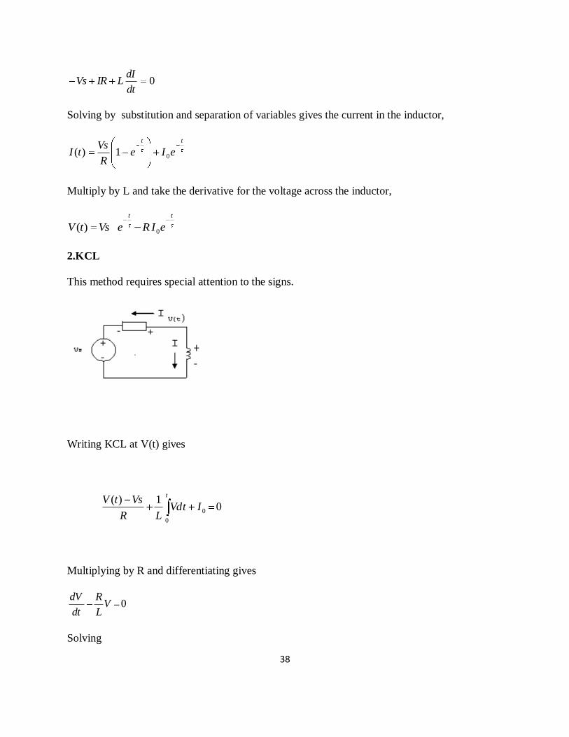
38

0dt

dILIRVs

Solving by substitution and separation of variables gives the current in the inductor,

tt

eIeR

VstI 01)(

Multiply by L and take the derivative for the voltage across the inductor,

tt

eIReVstV 0)(

2.KCL

This method requires special attention to the signs.

Writing KCL at V(t) gives

01)(

0

0

IVdtLR

VstVt

Multiplying by R and differentiating gives

0VL

R

dt

dV

Solving

39

t

eVtV 0)(

Vo is Vs plus the voltage across the resistor,

RIVsV sistorRe0 )0(

when Io is defined counter clockwise through the loop. This is different than the Io solved for in

I(t) by a sign.

sistorInductor II Re)0()0(

so,

t

eRIoVstV )()(

as before.

To find the current in the inductor,

)0(1

)(0

0 IeVL

tI

t t

where Io is defined through the inductor (opposite to the current in the resistor)

Doing the integration,

Inductor

t

Inductor

tt

t

t

IR

Ve

R

VtI

IeVR

L

LtI

)0()(

)0(1

)(

00

0

0

Remember,

InductorIRVsV )0(0

So for the inductor current,

40

InductorInductor

t

Inductor IR

IRVse

R

IRVstI )0(

)0()0()(

simplify,

tt

eIeR

VstI 01)(

3.Direct Substitution method

The driven response is also called the steady state or the particular solution. It is the final value

as t-> ∞

To solve

(3) 0dt

dILIRVs

assume steKKtI 21)( . K1 will carry the steady state response, the second term is the natural

response.

Substituting this assumption for I(t) into (3) and equating exponentials and constants each to 0

gives,

L

Rs

and

R

VsK1

Thus

t

eKR

VstI 2)(

At t=0 the current in the inductor is Io, so R

VsIK 02

giving

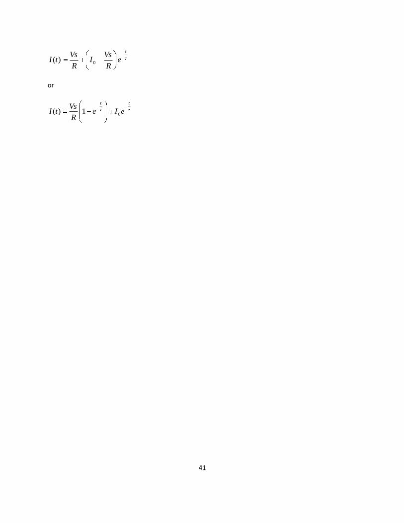
41

t

eR

VsI

R

VstI 0)(

or

tt

eIeR

VstI 01)(

42

APPENDIX B

AWG no Wire diam(mm)

Area ( ) AWG no Wire diam(mm)

Area ( )

0 8.25 53.4 19 0.912 0.653

1 7.35 42.4 20 0.812 0.519

2 6.54 33.6 21 0.723 0.412

3 5.83 26.7 22 0.644 0.325

4 5.19 21.2 23 0.573 0.259

5 4.62 16.8 24 0.511 0.205

6 4.11 13.3 25 0.455 0.163

7 3.67 10.6 26 0.405 0.128

8 3.26 8.35 27 0.361 0.102

9 2.91 6.62 28 0.321 0.0804

10 2.59 5.27 29 0.286 0.0646

11 2.3 4.15 30 0.255 0.0503

12 2.05 3.31 31 0.227 0.04

13 1.83 2.63 32 0.202 0.032

14 1.63 2.08 33 0.18 0.0252

15 1.45 1.65 34 0.16 0.02

16 1.45 1.31 35 0.143 0.0161

17 1.15 1.04 36 0.127 0.0123

18 1.024 0.823 37 0.113 0.01

AWG/ Metric conversion table

43

References

[1] F.W. Grover. Inductance Calculations - Working formulas and Tables. New York: Dover,

1978

[2] E. Rosa, “The self and mutual inductance of linear conductors,” in bulleting of the National

Bureau of standards, Vol. 4, pp. 301-344, 1908

[3] Marcelo A. Bueno and A.K.T. Assis. A new method for inductance calculations. Journal of

Physics D, 28;1802-1806,1995.

[4] J.d. Jackson. Classical Electrodynamics. John Wiley, New York, second edition, 1975.

[5] A.K.T. Assis. Weber’s Electrodynamics. Kluwer Academic Publishers, Dordrecht, 1994.

44