AIAA Numerical Simulation of Turbulent MHD Using an Iterative PNS … · 2013-08-30 · Numerical Simulation of Turbulent MHD Flows Using an Iterative PNS Algorithm Hiromasa Kato*

AIAA 2003-0326

Numerical Simulation of Turbulent MHD Flows Using an Iterative PNS Algorithm

Hiromasa Kat0 and John C. Tannehill, Iowa State University, Ames, IA 5001 1 and Unmeel B. Mehta NASA Ames Research Center, Moffett Field, CA 94035

41 st AIAA Aerospace Sciences Meeting and Exhibit

6-9 January 2003 / Reno, NV For permission to copy or republish, contact the copyright owner named on the first page. For AIAA-held copyright, write to AIAA, Permissions Department, 1801 Alexander Bell Drive, Suite 500, Reston, VA 20191-4344

https://ntrs.nasa.gov/search.jsp?R=20040105525 2019-07-20T16:56:29+00:00Z

Numerical Simulation of Turbulent MHD Flows Using an Iterative PNS Algorithm

Hiromasa Kato* and John C. Tannehillt Iowa State University, Ames, IA 50011

and Unmeel B. Mehtat

NASA Ames Research Center, Moflett Field, CA 94035

Abstract A new parabolized Navier-Stokes (PNS) algorithm has been developed to efficiently compute magnetohydrodynamic (MHD) flows in the low magnetic Reynolds number regime. In this regime, the electrical conductivity is low and the induced magnetic field is negligible compared to the applied magnetic field. The MHD effects are modeled by introducing source terms into the PNS equation which can then be solved in a very efficient manner. To account for upstream (elliptic) effects, the flowfields are computed using multiple streamwise sweeps with an iterated PNS algorithm. Turbulence has been included by modifying the Baldwin-Lomax turbulence model to account for MHD effects. The new algorithm has been used to compute both laminar and turbulent, supersonic, MHD flows over flat plates and supersonic viscous flows in a rectangular MHD accelerator. The present results are in excellent agreement with previous complete Navier-Stokes calculations.

Introduction Flowfields involving MHD effects have typically been computed [l-10) by solving the complete Navier- Stokes (N-S) equations for fluid flow in conjunction with Maxwell's equations of electromagnetodynam- ics. When chemistry and turbulence effects are also included, the computational effort required to solve the resulting coupled system of partial differential equations is extremely formidable. One possible rem- edy to this problem is to use the parabolized Navier-

*Graduate Research Assistant, Student Member AIAA t Manager, Computational Fluid Dynamics Center, and

:Division Scientist, Associate Fellow, AIAA

tics and Astronautics, Inc., all rights reserved.

Professor, Dept. of AEEM. Fellow AIAA

Copyright 0 2 0 0 3 by the American Institute of Aeronau-

Stokes (PNS) equations in place of the N-S equations. The PNS equations can be used to compute three-dimensional, supersonic viscous flowfields in a very efficient manner [ll]. This efficiency is achieved because the equations can be solved using a space- marching technique as opposed to the time-marching technique that is normally employed for the complete N-S equations.

Recently, the present authors have developed a PNS code to' solve supersonic MHD flowfields in the high magnetic Reynolds number regime [12]. This code is based on NASA's upwind PNS (UPS) code which was originally developed by Lawrence et al. [13]. The UPS code solves the PNS equations u s ing a fully conservative, finite-volume approach in a general nonorthogonal coordinate system. The UPS code has been extended to permit the computation of flowfields with strong upstream influences. In regions where strong upstream influences are present, the governing equations are solved using multiple sweeps. As a result of this approach, a complete flowfield can be computed more efficiently (in terms of computer time and storage) than with a standard N-S solver which marches the entire solution in time. Three iterative PNS algorithms (IPNS, TIPNS, and FBIPNS) have been developed. The iterated PNS (IPNS) algorithm [14] can be applied to flows with moder- ate upstream influences and small streamwise separated regions. The time iterated PNS (TIPNS) algorithm [15] can be used to compute flows with strong upstream influences including large streamwise s e p arated regions. The forward-backward sweeping iterative PNS (FBIPNS) algorithm [16] was recently developed to reduce the number of sweeps required for convergence.

The majority of MHD codes that have been developed combine the electromagnetodynamic equations with the full Navier-Stokes equations resulting in a complex system of eight scalar equations.

1 AMERICAN INSTITUTE OF AERONAUTICS AND ASTRONAUTICS

*. ..

These codes can theoreticdly be used for any magnetic Reynolds number which is defined as Re,,, = u,peV, L where 0; is the electrical conductivity, pe is the magnetic permeability, V, is the freestream velocity, and L is the reference length. However, it has been shown that as the magnetic Reynolds number is reduced, numerical difficulties are often encountered 241. For many aerospace applications the electrical conductivity of the fluid is low and hence the magnetic Reynolds number is small. In these cases, it makes sense to use the low magnetic Reynolds number assumption and reduce the com- plexity of the governing equations. In this case, the MHD effects can be modeled with the introduction of source terms into the fluid flow equations. Several investigators [4,8,17-191 have developed N-S codes for the low magnetic Reynolds number regime where the induced magnetic field is negligible compared to the applied magnetic field.

In the present study, a new PNS code (based on the UPS code) has been developed to compute MHD flows in the low magnetic Reynolds number regime. The MHD effects are modeled by introducing the a p propriate source terms into the PNS equations. U p stream elliptic effects can be accounted for by u s ing multiple streamwise sweeps with either the IPNS, TIPNS, or FBIPNS algorithms. Turbulence has been included by modifying the Baldwin-Lomax turbulence model [20] to account for MHD effects using the approach of Lykoudis [21]. The new code has been tested by computing both laminar and turbulent, supersonic MHD flows over a flat plate. Com- parisons have been made with the previous complete N-S computations of Dietiker and H o h a n n [MI. In addition, the new code has been used to compute the supersonic viscous flow inside a rectangular channel designed for MHD experiments [22].

Governing Equations The governing equations for a viscous MHD flow with a small magnetic Reynolds number are given by [18]: Continuity equation

aP - + V . ( p V ) = o at Momentum equation

Energy equation

Ohm's law J = ue (E + V x B) (4)

where V is the velocity vector, B is the magnetic field vector, E is the electric field vector, and J is the conduction current density. The flow is assumed to be either in chemical equilibrium or in a frozen state. The curve fits of Srinivasan et al. [23,24] are used for the thermodynamic and transport properties of equilibrium air.

The governing equations are nondimensionalized using the following reference variables.

U , V , W umt , t =- L X,Y,Z , u* ,v * ,w* = - x*,y*,z = -

L urn

p * P =- , T=-, T pa=--- P Pm T, Pm E et =* 5L , / A * = - Ir (5) ef = - , r = -

@a P a UCQ Pm

where the superscript * refers to the nondimensional quantities. In subsequent sections, the asterisks are dropped.

If the flow variables are assumed to vary in only two dimensions (2, y) while the velocity, magnetic, and electric fields have components in three dimensions (2 , y, z ) , the governing equations can be written in the following flux vector form:

aU aEi aFi aEu dFu -+-+-=- +-+SMHD ( 6 )

where U is the vector of dependent variables and E; and Fi are the inviscid flux vectors, and E,, and Fu are the viscous flux vectors. The source term SMHD contains all of the MHD effects. The flux vectors are given by

at ax ay az ay


F, = I 0 1 &(Ey + wBz - uB,)

-&(Ey + wBz - uB,) Ez(Ez + vB, - wB,) +Ey(Ey + wB, - uB,) +Ez(E, + uBY - vB,)

where

1 P Pet = Z P (u2 + v2 + W Z ) + - 7 - 1

and 7 can be determined from the curve fits of Srini- vasan et al. [23] for an equilibrium air flow or is equal to a constant (7) for a frozen or perfect gas flow. The nondimensional shear stresses and heat fluxes are defined in the usual manner [ll].

The governing equations are transformed into computational space and written in a generalized coordinate system ( t ,~) as

where

and J is the Jacobian of the transformation. The governing equations are parabolized by drop

ping the time derivative term and the streamwise direction ( E ) viscous flow terms in the flux vectors. Equation (13) can then be rewritten as

where

= (9) (Ei -E:) + (9) (Fi -FL) (16)

The prime in the preceding equation indicates that the streamwise viscous flow terms have been dropped.

For turbulent flows, the two-layer Baldwin-Lomax turbulence model [20] has been modified to account for MHD effects. Only the expression for turbulent viscosity in the inner layer is changed. This modifi- cation for MHD flows is due to Lykoudis [9,21].

Numerical Met hod The governing PNS equations with MHD source terms have been incorporated into NASA’s upwind PNS (UPS) code 1131. These equations can be solved very efficiently using a single sweep of the flowfield for many applications. For cases where upstream (elliptic) effects are important, the flowfield can be computed using multiple streamwise sweeps with either the IPNS [14], TIPNS [15], or FBIPNS [16] algorithms. This iterative process is continued until the solution is converged.

For the iterative PNS (IPNS) method, the E vector is split using the Vigneron parameter (w) [25]. This parameter does not need to be changed for the present low magnetic Reynolds number formulation. In the previous high magnetic Reynolds number code [12] it was necessary to modify the Vigneron parameter to account for MHD effects. After splitting, the E vector can be written as:

E = E ’ + W (17) where

Ep

- Pu2 +WP 1

FY + - J

The streamwise derivative of E is then differenced using a forward difference for the “elliptic” portion (W:


.I ..

where the subscript (i + 1) denotes the spatial index (in the direction) where the solution is currently being computed. The vectors ET+l and are then linearized in the following manner:

The Jacobians can be represented by

After substituting the above linearizations into Eq. (19), the expression for the streamwise gradient of E becomes

(22)

The final discretized form of the fluid flow equations with MHD source terms is obtained by substituting Eq. (22) into J3q. (15) along with the linearized expression for the flux in the cross flow plane. The final expression becomes:

[&(A;

= RHS (23)

where

1 RHS = -- - A<

and the superscript k+l denotes the current iteration (Le. sweep) level.

Numerical Results In order to investigate the utility and accuracy of the present PNS approach of solving MHD flowfields at low magnetic Reynolds numbers, a few basic test cases were computed. The supersonic viscous flow in these cases is altered by the presence of the magnetic and electric fields which are applied to the flow.

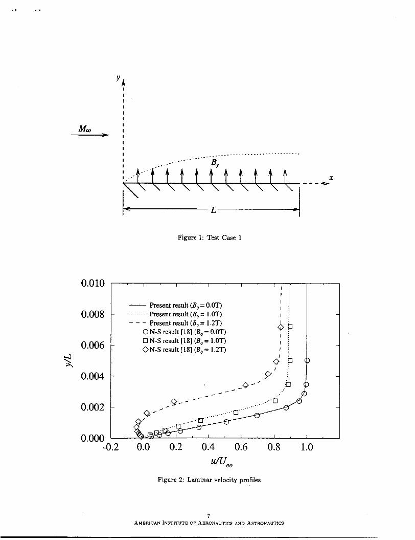
Test Case 1: Supersonic laminar and turbulent flows over a flat plate with applied magnetic field In this test case, the supersonic, laminar and turbulent flow over a flat plate with an applied magnetic field is computed. This case corresponds to the flat plate case computed previously by Dietiker and Hoff- mann [18] using the full N-S equations. A strong magnetic field is applied normal to the flow as shown in Fig. 1. The dimensional flow parameters for this test case are:

M , = 2.0 pa, = 1.076 x lo5 N/m2 T, = 300K Re, = 3.75 x lo6

7 = 1.4 L = 0.08 m u, = 800mho/m

The plate is assumed to be an adiabatic wall and a perfect gas flow is assumed. The magnetic Reynolds number (based on the length of the plate) is 0.056 and can be considered negligible when compared to one. The normal magnetic field component (By) ranges in value from 0.0 to 1.2 T. The magnitude of the magnetic field can be represented by the parameter m which is defined [I81 by

ue B2 m = Y (24) Po0 urn

and has units of ( l /m) . For By = 1.2 T, m is equal to 1.33.

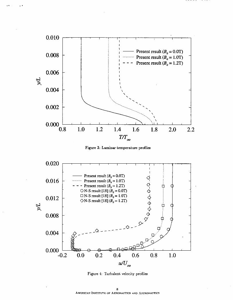
A highly stretched grid consisting of 50 points in the normal direction was used to compute this case. The first point off the wall was located at 2 x m. Initially, the flow was assumed laminar and several values of By ranging from 0.0 (no magnetic field) to 1.2 T were used. The velocity and temperature profiles at z = 0.06 m are shown in Figs. 2 and 3 for By = 0.0 T, 1.0 T, and 1.2 T. The velocity profiles are compared to the N-S results of Dietiker and Hoff- mann in Fig. 2 and show excellent agreement. The magnetic field generates a Lorentz force which acts in a direction opposite to the flow. Thus, the flow is de- celerated as the magnetic field is increased as seen in Fig. 2. For By = 1.2 T the flow is slightly separated. The temperature profiles cannot be compared at this time since no temperature data is given in Ref. 1181.

The turbulent flow over the flat plate was then computed using the modified Baldwin-Lomax turbulence model that accounts for MHD effects. The flow


.. ..

was assumed laminar prior to the point (z = 0.04 m) where transition from laminar to turbulent flow was triggered. Again, several values of By ranging from 0.0 to 1.2 T were used in the computations. The turbulent velocity and temperature profiles at z = 0.06 m are shown in Figs. 4 and 5 for By = 0.0, 1.0 T, and 1.2 T. The turbulent velocity profiles in Fig. 4 are in good agreement with the results of Ref. [18]. The variation of skin friction coefficient is shown in Fig. 6. The present laminar/turbulent skin friction variations are compared with the results of Ref. [18] and show good agreement. The difference in results near the transition point may be due to the coarse grid and smoothing used in Ref. [l8].

All of the present laminar computations were performed using a single sweep of the flowfield except for the separated flow case (By = 1.2 T). For this case as well as for all the turbulent cases, multiple sweeps were used to account for upstream effects.

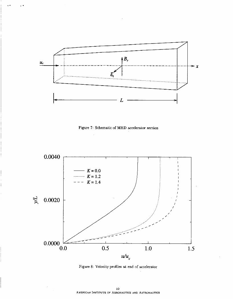
Test Case 2: Supersonic viscous flow in a rectangular MHD accelerator In this test case, the supersonic flow in an experimental MHD channel is simulated. This facility is currently being built at NASA Ames Research Center by D. W. Bogdanoff, C. Park, and U. B. Mehta [22] to study critical technologies related to MHD bypass scramjet engines. The channel is about a half meter long and contains a nozzle section, a center section, and an accelerator section. The channel has a uni- form width of 2.03 cm. Magnetic and electric fields can be imposed upon the flow in the accelerator section. A schematic of the MHD accelerator section is shown in Fig. 7.

This test case was previously computed by R. W. MacCormack [lo] using the full N-S equations coupled with the electromagnetodynamic equations. The electrical conductivity in his calculations was set at 1.0 x lo5 mho/m resulting in avery large magnetic Reynolds number. In the present study, the calculations are performed in the low magnetic Reynolds number regime using a realistic value of electrical conductivity. The flow is computed in two dimensions, but later will be extended to three dimensions. Be- cause of flow symmetry, only half of the channel is computed in the 2-D calculations.

The flow in the nozzle section and the center section was computed using a combination of the OVER- FLOW code [26] and the present PNS code (without MHD effects). The initial conditions for the nozzle (flow at rest) were:

PO = 8.0 x lo5 N/m2

To = 7500 K

The laminar flow was assumed to be in chemical equilibrium. The computed flowfield at the end of the center section was then used as the starting solution for the flow calculation of the accelerator section. The MHD parameters used in the accelerator section were:

u, = 50 mho/m By = 1.5 T E, = -Ku,By

Re,,, = 0.05

where the load factor ( K ) ranged in values from 0.0 to 1.4, and the centerline velocity (ue) at the beginning of the accelerator section had a value of 3162 m/s.

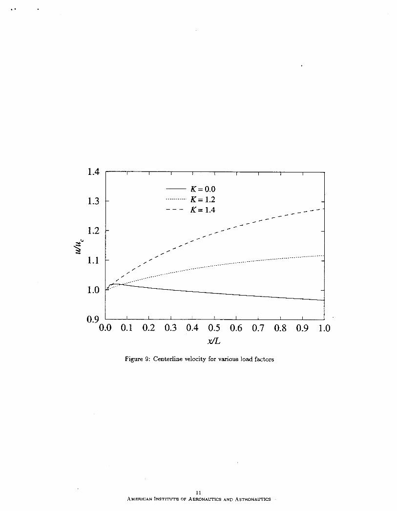
The velocity profiles at the end of the accelerator section are shown in Fig. 8 for different load factors. The velocity profile with no electric or magnetic fields is denoted by K = 0. The increase in the centerline velocity with distance (z) for various load factors is shown in Fig. 9. The centerline velocity increases by about 30% with a load factor of 1.4. It should be noted that the flow decelerates because of friction when no electric or magnetic fields are applied.

Concluding Remarks In this study, a new parabolized Navier-Stokes algorithm has been developed to efficiently compute MHD flows in the low magnetic Reynolds number regime. The new algorithm has been used to compute both laminar and turbulent, supersonic, MHD flows over flat plates and in a rectangular accelerator section. Although only limited results have been obtained thus far, it can be seen that the present approach is quite promising. Computations of other test cases are currently underway in order to validate the current method.

Acknowledgments This work was supported by NASA Amea Fbsearch Center under Grants NCC2-53T9 and NCC2-5517 and by Iowa State UniversiQ. The Technical Mon- itor for the NASA grant is Dr. Unmeel B. Mehta

References [l] Gaitonde, D. V., “Development of a Solver for 3-

D Non-Ideal Magnetogasdynamics,” AIAA Pa- per 99-3610, June 1999.


.. ..

Damevin, H. M., Dietiker, J.-F., and Hoffmann, K. A., “Hypersonic Flow Computations with Magnetic Field,” A M Paper 2000-0451, Jan. 2000.

Hoffmann, K. A., Damevin, H. M., and Di- etiker, J.-F., “Numerical Simulation of Hyper- sonic Magnetohydrodynamic Flows,” AIAA Pa- per 2000-2259, June 2000.

Gaitonde, D. V. and Poggie, J., “Simulation of MHD Flow Control Techniques,” AIAA Paper 2000-2326, June 2000.

MacCormack, R. W., ”Numerical Computa- tion in Magnetofluid Dynamics,” Computational Fluid Dynamics for the 21st Century, Kyoto, Japan, July 2000.

Deb, P. and Agarwal, R., “Numerical Study of MHD-Bypass Scramjet Inlets with Finite-Rate Chemistry,” AIAA Paper 2001-0794, Jan. 2001.

MacCormack, R. W., “A Computational Method for Magneto-Fluid Dynamics,” AIAA Paper 2001-2735, June 2001.

Gaitonde, D. V. and Poggie, J., “An Implicit Technique for 3-D Turbulent MGD with the Generalized Ohm’s Law,” AIAA Paper 2001- 2736, June 2001.

Dietiker, J.-F. and Hoffmann, K. A., “Numerical Simulation of Turbulent Magnetohydrodynamic Flows,” AIAA Paper 2001-2737, June 2001.

MacCormack, R. W., “Three Dimensional Magneto-Fluid Dynamics Algorithm Develop ment,” AIAA Paper 2002-0197, Jan. 2002.

Tannehill, J. C., Anderson, D. A., and Pletcher, R. H., Computational Fluid Mechanics and Heat Transfer, Taylor and Francis, Washington, D.C., 1997 .

[12] Kato, H., Tannehill, J . C., Ramesh, M. D., and Mehta, U. B., “Computation of Magnetohydro- dynamic Flows Using an Iterative PNS Algo- rithm,” AIAA Paper 2002-0202, Jan. 2002.

[13] Lawrence, S. L., Tannehill, J . C., and Chaussee, D. S., “Upwind Algorithm for the Parabo- lized Navier-Stokes Equations,” AIAA Journal, Vol. 27, No. 9, Sept. 1989, pp. 1975-1983.

[14] Miller, J . H., Tannehill, J. C., and Lawrence, S. L., “PNS Algorithm for Solving Supersonic Flows with Upstream Influences,” AIAA Paper 98-0226, Jan. 1998.

[15] Tannehill, J. C., Miller, J. H., and Lawrence, S. L., “Development of an Iterative PNS Code for Separated Flows,” AIAA Paper 99-3361, June 1999.

[16] Kato, H. and Tannehill, J. C., “Development of a Forward-Backward Sweeping Parabolized Navier-Stokes Algorithm,” AIAA Paper 2002- 0735, Jan. 2002.

[17] Munipalli, R., Anderson, D. A., and Kim, H., “Two-Temperature Computations of Ionizing Air with MHD Effects,” AIAA Paper 2000-0450, Jan. 2000.

[18] Dietiker, J.-F. and Hoffmann, K. A., “Boundary Layer Control in Magnetohydrodynamic Flows,” AIAA Paper 2002-0130, Jan. 2002.

[19] Cheng, F., Zhong, X., Gogineni, S., andKimmel, R. L., “Effect of Applied Magnetic Field on the Instability of Mach 4.5 Boundary Layer over a Flat Plate,” AIAA Paper 2002-0351, Jan. 2002.

[20] Baldwin, B. S. and Lomax, H., Thin Layer Approximation and Algebraic Model for S e p arated Turbulent Flows,” AIAA-Paper 78-257, Jan. 1978.

[21] Lykoudis, P. S., “Magneto Fluid Mechanics Channel Flow, I1 Theory,” The Physics of FZu- ids, Vol. 10, No. 5, May 1967, pp- 1002-1007.

[22] Bogdanoff, D. W., Park, C., and Mehta, U. B., “Experimental Demonstration of Magnet* Hydrodynamic (MHD) Acceleration - Facility and Conductivity Measurements,” NASA TM- 2001-210922, July 2001.

[23] Srinivasan, S., Tannehill, J. C., and Weilmuen- ster, K. J., “Simplified Curve Fits for the Thermodynamic Properties of Equilibrium Air,” NASA RP 1181, Aug. 1987.

[24] Srinivasan, S., Tannehill, J . C., and Weilmuen- ster, K. J., “Simplified Curve Fits for the Trans port Properties of Equilibrium Air,” NASA CR 178411, 1987.

[25] Vigneron, Y. C., Rakich, J. V., and Tan- nehill, J. C., “Calculation of Supersonic Flow over Delta Wings with Sharp Subsonic Leading Edges,” AIAA Paper 78-1137, July 1978.

[26] Buning, P. G., Jespersen, D. C., and Pulliam, T. H., OVERFLOW Manual, Version 1.7v, NASA Ames Research Center, Moffett Field, California, June 1997.


.. ..

Y A I

I I I I I I Ma, I

- 1 I I

0.010

0.008

0.006 4 k

0.004

0.002

0.000

Figure 1: Test Case 1

I I I I I .' I i I l j I j

I ! Present result (Bo = 0.0") Present result (Bo = 1.0")

0 N-S result [ 181 (Bo = 1 .On ON-S result [lS] (Bo= 1.2")

I : I .

I :

1 ; I ;

. - - - - -

0 0 - - - Present result (Bo = 1.2") 0 N-S result [ 181 (Bo = 0.0")

-0.2 0.0 0.2 0.4 0.6 0.8 1 .o n o 0

Figure 2: Laminar velocity profiles


.. . -

0.010

0.008

0.006

0.004

0.002

I ' ' I I I I I I

I !

I Present result (Bo = 0.OT) I - - - - - - - - - - Present result (Bo = 1.OT) - - - Present result (Bo = 1.2T)

i I I I I I I I \ \ \ \

I I I I \ I : I \ I I O.Oo0 0.8 1.0 1.2 1.4 1.6 1.8 2.0 2.2

Figure 3: Laminar temperature profiles

I I I I I 1 I 1 I

0.020 I

I 0.016

0.012 1 i- 4 k

0.004

0.0°8 ~

I Present result (Bo = 0.OT) Present result (Bo = 1 .OT)

- - - Present result (Bo = 1.2T)

___. _.__

0 cp

I 0 N-S result [18] (Bo = 0.OT)

4 ; 0 N-S result [18] (Bo = 1.OT) ON-S result [ 181 (Bo = 1.2T)

0

0.000 -0.2 0.0 0.2 0.4 0.6 0.8 1 .o

n o 0

Figure 4: Turbulent velocity profiles

8 AMERICAN INST!,TUTE OF AERONAUTICS AND ASTRONAUTICS

0.0020

0.0016

0.0012

O.Ooo8

O.OOO4

O.oo00

0.003

0.002

0.001

0.000

I : # I I I I I

I

1 - I Present result (Bo = 0.OT) I _ _ _ _ _ _ _ _ _ _ Present result (Bo = 1.OT). I - - - Present result (Bo = 1.2T) I I I I I I I \ \ \ \ \ \ \ \

0.8 1.0 1.2 I .4 1.6 1.8 2.0 2.2

Figure 5: Turbulent temperature profiles

I I I

Present result (Bo = 0.0T) - - . - - - - - Present result (Bo = 1.OT) - - - Present result (Bo = 1.2T)

0 N-S result [18] (Bo = 0.OT) CI N-S result [18] (Bo = 1.OT) 0 N-S result [18] (Bo = 1.2T)

4 I

0.00 0.02 0.04 x, m

0.06

Figure 6: Laminar/turbulent skin friction coefficient

0.08


I I

Figure 7: Schematic of MHD accelerator section

0.0040

k 0.0020

K = 0.0 K = 1.2 K = 1.4

/ I

0.0000 0.0 0.5 1 .o 1.5

U/U C

Figure 8: Velocity profiles at end of accelerator


K = 0.0 K = 1.2 ._-_______ - K = 1.4

. I , .

i ________/ 0.9 I I I I I I I I I I 1

0.0 0.1 0.2 0.3 0.4 0.5 0.6 0.7 0.8 0.9 1.0 IdL

Figure 9: Centerline velocity for various load factors


Documents

AIAA Numerical Simulation of Turbulent MHD Using an Iterative PNS … · 2013-08-30 · Numerical Simulation of Turbulent MHD Flows Using an Iterative PNS Algorithm Hiromasa Kato*