Embed Size (px)
Citation preview
AI in Actuarial Science Ronald Richman

AGENDA
1. Introduction
2. Background
• Machine Learning
• Deep Learning
• Five Main Deep Architectures
3. Applications in Actuarial Science
4. Discussion and Conclusion
01
PG 1

INTRODUCTION
02
PG 2
This talk is about 3 things:
1.Provide context to understand deep learning
2.Discuss applications of deep learning in actuarial
science
3.Provide code to experiment (see last slide)
And also…

THE SHIP IS SAIL ING 03
PG 3
WHAT INSPIRED THIS TALK? (1)
04
PG 4
"The future of insurance will be staffed by bots
rather than brokers and AI in favor of actuaries"-
Daniel Schreiber, Lemonade Inc.
WHAT INSPIRED THIS TALK? (2)
05
PG 5
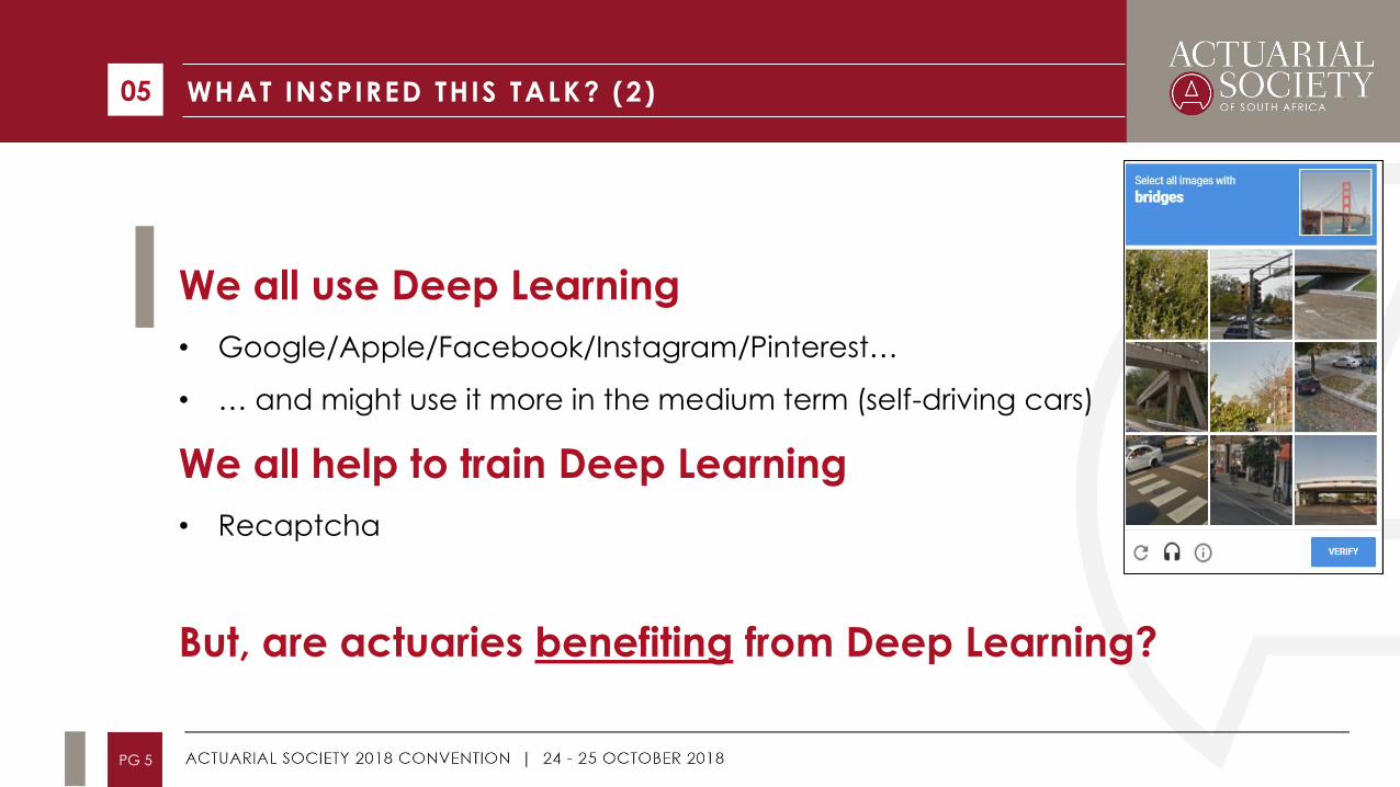
We all use Deep Learning
• Google/Apple/Facebook/Instagram/Pinterest…
• … and might use it more in the medium term (self-driving cars)
We all help to train Deep Learning
• Recaptcha
But, are actuaries benefiting from Deep Learning?
AGENDA
1. Introduction
2. Background
• Machine Learning
• Deep Learning
• Five Main Deep Architectures
3. Applications in Actuarial Science
4. Discussion and Conclusion
06
PG 6
MACHINE LEARNING
Machine Learning is the field concerned with “the study of algorithms that allow computer
programs to automatically improve through experience” (Mitchell 1997)
• Machine learning approach to AI - systems trained to recognize patterns within data to
acquire knowledge (Goodfellow, Bengio and Courville 2016).
• Different paradigm from earlier attempts to build AI systems:
• Hard coding knowledge into knowledge bases to solve problems in formal domains
defined by mathematical rules.
• Highly complex tasks e.g. image recognition, scene understanding and inferring
semantic concepts (Bengio 2009) more difficult to solve for AI systems.
• ML Paradigm – feed data to the machine and let it figure it out!
07
PG 7
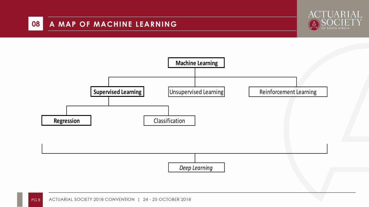
A MAP OF MACHINE LEARNING 08
PG 8
Reinforcement Learning
Regression
Deep Learning
Machine Learning
Unsupervised LearningSupervised Learning
Classification

SUPERVISED LEARNING (1)
Supervised learning = application of machine learning to datasets that contain
features and outputs with the goal of predicting the outputs from the features
(Friedman, Hastie and Tibshirani 2009).
09
PG 9
X (features) y (outputs)
More on the French MTPL dataset later.
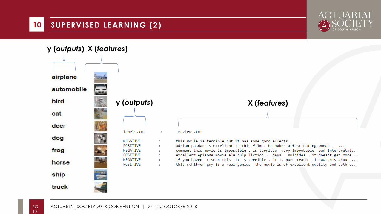
SUPERVISED LEARNING (2) 10
PG
10
X (features) y (outputs)
X (features) y (outputs)
UNSUPERVISED LEARNING
Unsupervised learning = application of machine learning to datasets
containing only features to find structure within these datasets (Sutton and
Barto 2018). Task of unsupervised learning is to find meaningful patterns
using only the features.
• Recent example - modelling yield curves using Principal Components
Analysis (PCA) for the Interest Rate SCR in SAM
• Mortality modelling – Lee-Carter model uses PCA to reconstruct mortality
curves
11
PG
11

REINFORCEMENT LEARNING
Reinforcement learning = learning action to take in situations in order for an
agent to maximise a reward signal (Sutton and Barto 2018).
12
PG
12
ML AND ACTUARIAL PROBLEMS
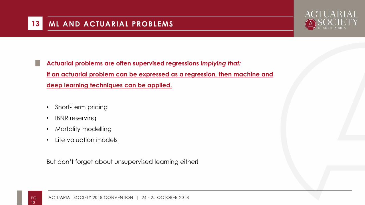
Actuarial problems are often supervised regressions implying that:
If an actuarial problem can be expressed as a regression, then machine and
deep learning techniques can be applied.
• Short-Term pricing
• IBNR reserving
• Mortality modelling
• Lite valuation models
But don’t forget about unsupervised learning either!
13
PG
13
SO, ML IS JUST REGRESSION, RIGHT?
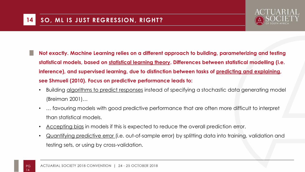
Not exactly. Machine Learning relies on a different approach to building, parameterizing and testing
statistical models, based on statistical learning theory. Differences between statistical modelling (i.e.
inference), and supervised learning, due to distinction between tasks of predicting and explaining,
see Shmueli (2010). Focus on predictive performance leads to:
• Building algorithms to predict responses instead of specifying a stochastic data generating model
(Breiman 2001)…
• … favouring models with good predictive performance that are often more difficult to interpret
than statistical models.
• Accepting bias in models if this is expected to reduce the overall prediction error.
• Quantifying predictive error (i.e. out-of-sample error) by splitting data into training, validation and
testing sets, or using by cross-validation.
14
PG
14
AGENDA
1. Introduction
2. Background
• Machine Learning
• Deep Learning
• Five Main Deep Architectures
3. Applications in Actuarial Science
4. Discussion and Conclusion
15
PG
15
FEATURE ENGINEERING
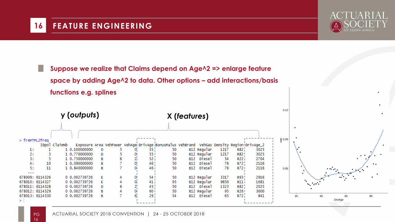
Suppose we realize that Claims depend on Age^2 => enlarge feature
space by adding Age^2 to data. Other options – add interactions/basis
functions e.g. splines
16
PG
16
X (features) y (outputs)
0.06
0.09
0.12
20 40 60 80
DrivAge
rate

REPRESENTATION LEARNING
In many domains, including actuarial science, traditional approach to designing
machine learning systems relies on humans for feature engineering. But:
• designing features is time consuming/tedious
• relies on expert knowledge that may not be transferable to a new domain
• becomes difficult with very high dimensional data
Representation (feature) Learning = machine learning approach that allows
algorithms automatically to design a set of features that are optimal for a
particular task. Traditional examples:
• Unsupervised = PCA
• Supervised = PLS
Simple/naive RL approaches often fail when applied to high dimensional data
17
PG
17
DEEP LEARNING (1)
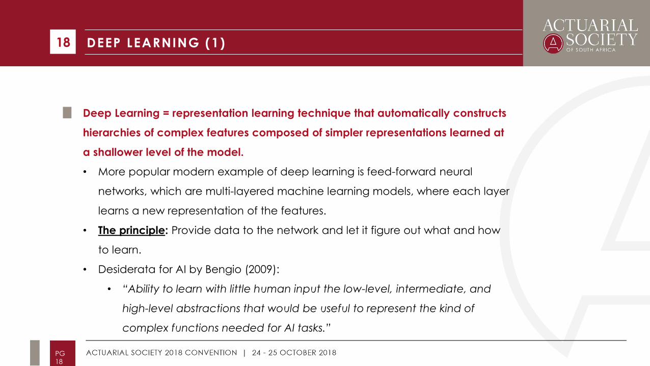
Deep Learning = representation learning technique that automatically constructs
hierarchies of complex features composed of simpler representations learned at
a shallower level of the model.
• More popular modern example of deep learning is feed-forward neural
networks, which are multi-layered machine learning models, where each layer
learns a new representation of the features.
• The principle: Provide data to the network and let it figure out what and how
to learn.
• Desiderata for AI by Bengio (2009):
• “Ability to learn with little human input the low-level, intermediate, and
high-level abstractions that would be useful to represent the kind of
complex functions needed for AI tasks.”
18
PG
18
DEEP LEARNING (2)
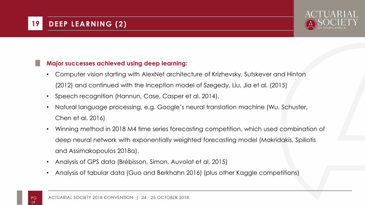
Major successes achieved using deep learning:
• Computer vision starting with AlexNet architecture of Krizhevsky, Sutskever and Hinton
(2012) and continued with the Inception model of Szegedy, Liu, Jia et al. (2015)
• Speech recognition (Hannun, Case, Casper et al. 2014).
• Natural language processing, e.g. Google’s neural translation machine (Wu, Schuster,
Chen et al. 2016)
• Winning method in 2018 M4 time series forecasting competition, which used combination of
deep neural network with exponentially weighted forecasting model (Makridakis, Spiliotis
and Assimakopoulos 2018a).
• Analysis of GPS data (Brébisson, Simon, Auvolat et al. 2015)
• Analysis of tabular data (Guo and Berkhahn 2016) (plus other Kaggle competitions)
19
PG
19
AGENDA
1. Introduction
2. Background
• Machine Learning
• Deep Learning
• Five Main Deep Architectures
3. Applications in Actuarial Science
4. Discussion and Conclusion
20
PG
20
DEEP FEEDFORWARD NET 21
PG
21
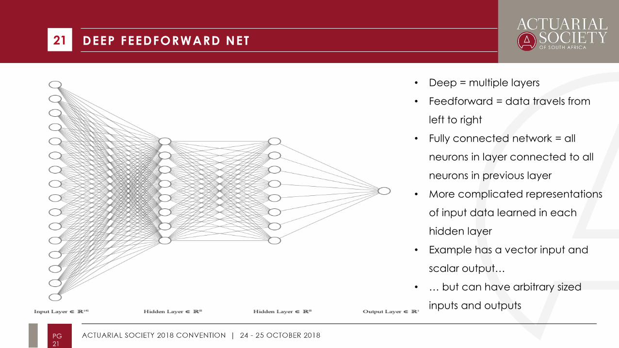
• Deep = multiple layers
• Feedforward = data travels from
left to right
• Fully connected network = all
neurons in layer connected to all
neurons in previous layer
• More complicated representations
of input data learned in each
hidden layer
• Example has a vector input and
scalar output…
• … but can have arbitrary sized
inputs and outputs

DEEP AUTOENCODER 22
PG
22
• Deep = multiple layers
• Autoencoder = network is trained
to produce output equal to the
input
• Vector input and output
• Bottleneck in middle restricts
dimension of encoded data…
• … in this example, to 1, but can be
to multiple dimensions
• Performs a type of non-linear PCA
• Encoded data summarizes the
input
CONVOLUTIONAL NEURAL NETWORK 23
PG
23
0 0 0 0 0 0 0 0 0 0
0 0 0 3 4 4 4 1 0 0
0 0 1 3 0 0 1 4 0 0
0 0 3 0 0 3 4 1 0 0
0 1 0 0 1 4 2 1 0 0 1 1 1
= 0 0 0 1 4 2 1 0 0 0 0 0 0
0 0 1 4 1 1 0 0 0 0 -1 -1 -1
0 0 4 4 4 4 4 4 0 0
0 0 0 0 0 0 0 0 0 0
0 0 0 0 0 0 0 0 0 0 0*1 0*1 0*1 0 0 0
0*0 0*0 0*0 = 0 0 0 = -1
-1 -4 -4 -3 -1 -5 -5 -4 0*-1 0*-1 1*-1 0 0 -1
-3 0 4 8 5 1 0 0
0 3 3 -2 -6 -2 2 3
3 2 -2 -4 0 5 4 1
0 -4 -5 -1 5 6 3 1
-4 -7 -7 -5 -5 -9 -7 -4
1 5 6 6 2 1 0 0
4 8 12 12 12 12 8 4
Filter
Data Matrix
Feature Map
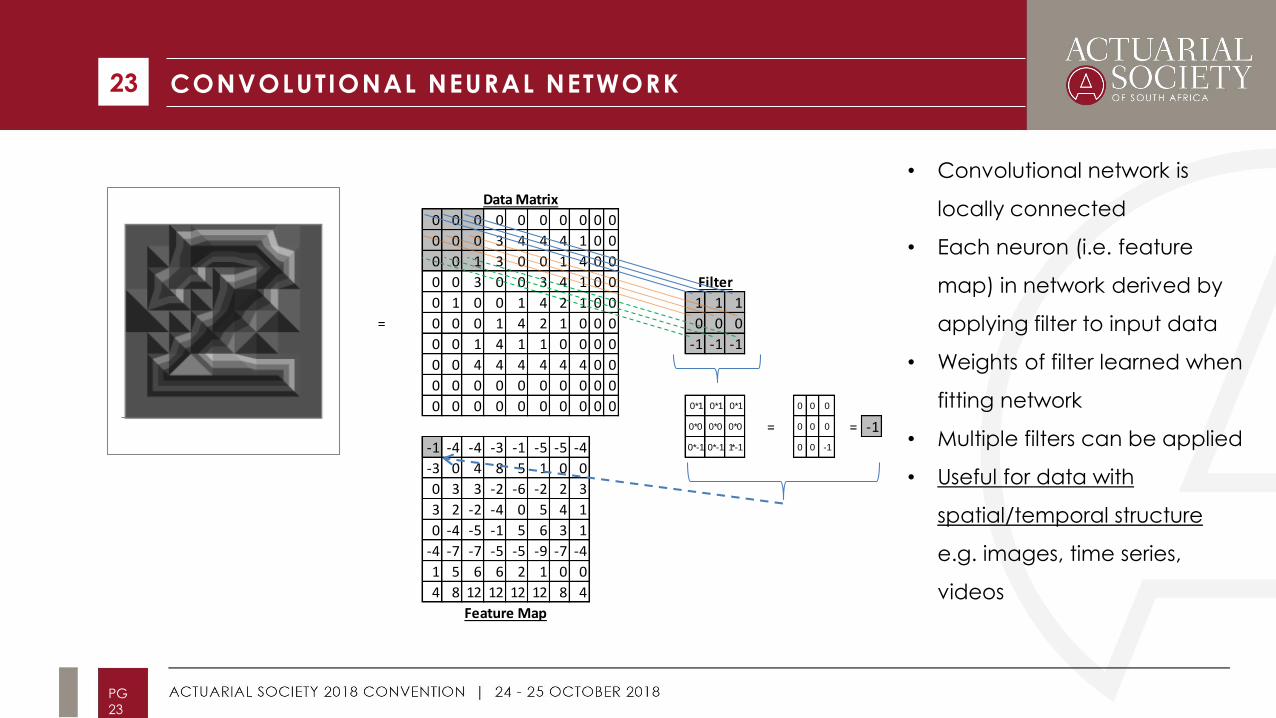
• Convolutional network is
locally connected
• Each neuron (i.e. feature
map) in network derived by
applying filter to input data
• Weights of filter learned when
fitting network
• Multiple filters can be applied
• Useful for data with
spatial/temporal structure
e.g. images, time series,
videos
RECURRENT NEURAL NETWORK 24
PG
24
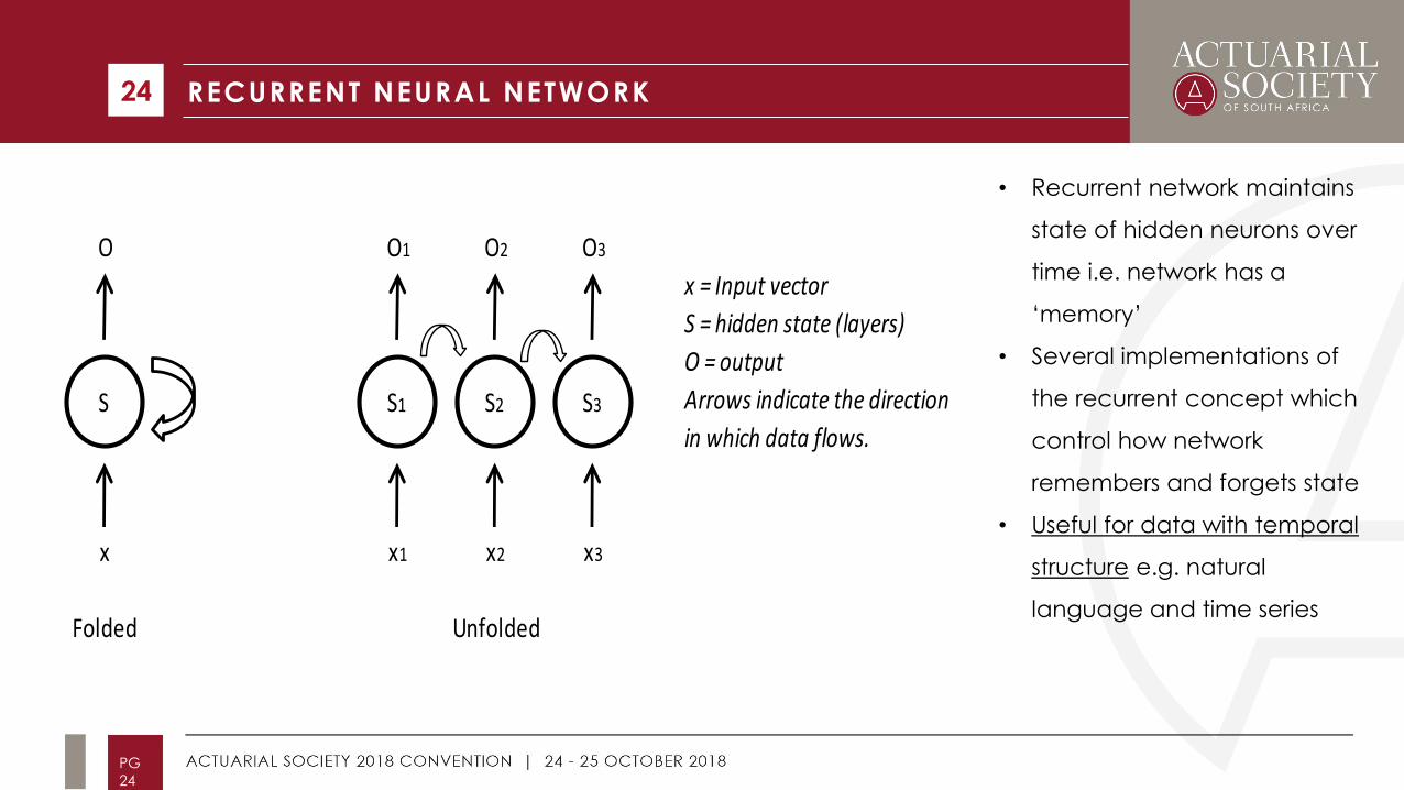
O O1 O2 O3
x = Input vector
S = hidden state (layers)
O = output
Arrows indicate the direction
in which data flows.
x x1 x2 x3
Folded Unfolded
S S1 S2 S3
• Recurrent network maintains
state of hidden neurons over
time i.e. network has a
‘memory’
• Several implementations of
the recurrent concept which
control how network
remembers and forgets state
• Useful for data with temporal
structure e.g. natural
language and time series
EMBEDDING LAYER 25
PG
25
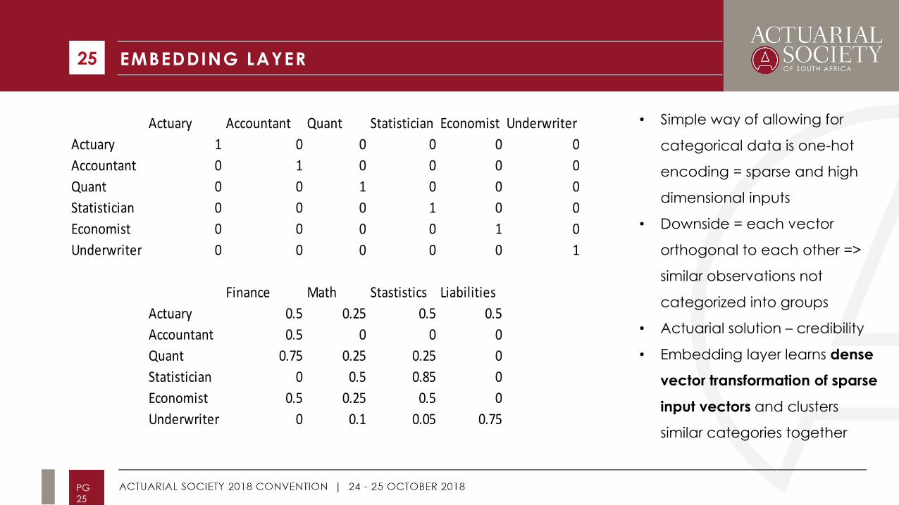
Actuary Accountant Quant Statistician Economist Underwriter
Actuary 1 0 0 0 0 0
Accountant 0 1 0 0 0 0
Quant 0 0 1 0 0 0
Statistician 0 0 0 1 0 0
Economist 0 0 0 0 1 0
Underwriter 0 0 0 0 0 1
Finance Math Stastistics Liabilities
Actuary 0.5 0.25 0.5 0.5
Accountant 0.5 0 0 0
Quant 0.75 0.25 0.25 0
Statistician 0 0.5 0.85 0
Economist 0.5 0.25 0.5 0
Underwriter 0 0.1 0.05 0.75
• Simple way of allowing for
categorical data is one-hot
encoding = sparse and high
dimensional inputs
• Downside = each vector
orthogonal to each other =>
similar observations not
categorized into groups
• Actuarial solution – credibility
• Embedding layer learns dense
vector transformation of sparse
input vectors and clusters
similar categories together
SUMMARY OF ARCHITECTURES
26
PG
26
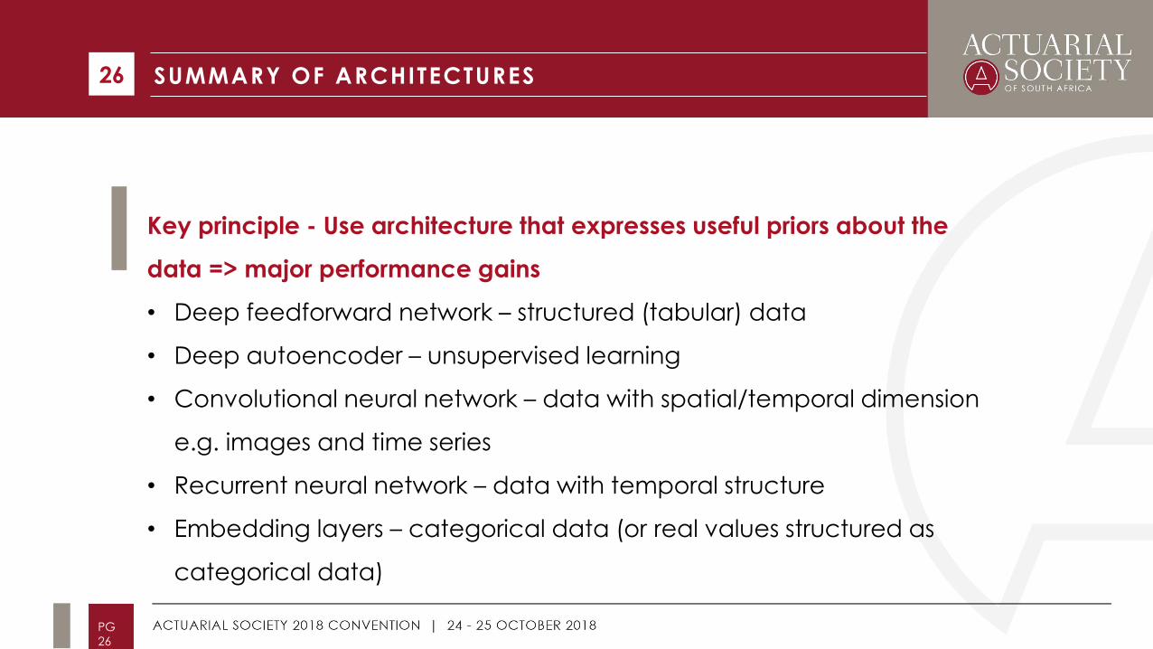
Key principle - Use architecture that expresses useful priors about the
data => major performance gains
• Deep feedforward network – structured (tabular) data
• Deep autoencoder – unsupervised learning
• Convolutional neural network – data with spatial/temporal dimension
e.g. images and time series
• Recurrent neural network – data with temporal structure
• Embedding layers – categorical data (or real values structured as
categorical data)
AGENDA
1. Introduction
2. Background
• Machine Learning
• Deep Learning
• Five Main Deep Architectures
3. Applications in Actuarial Science
4. Discussion and Conclusion
27
PG
27
APPLICATIONS IN ACTUARIAL SCIENCE
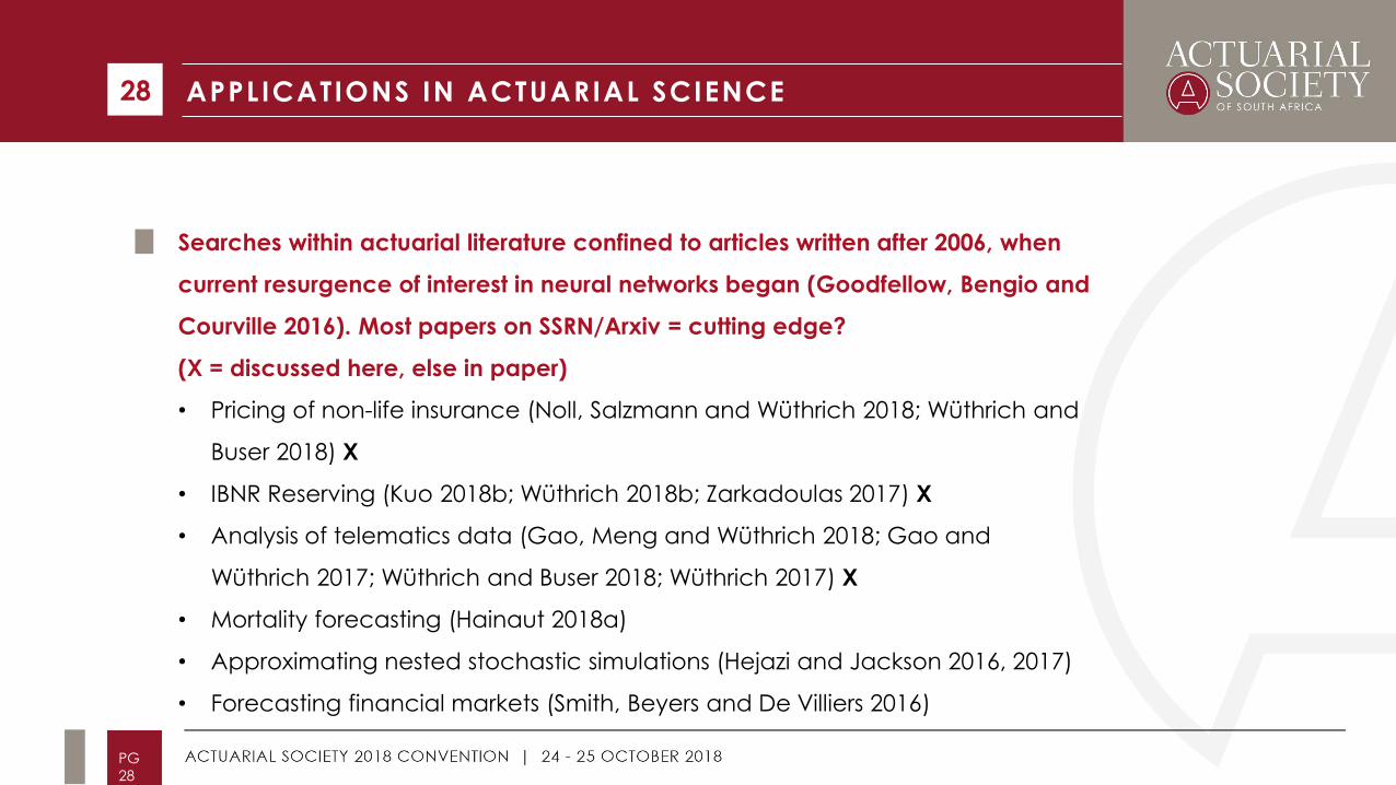
Searches within actuarial literature confined to articles written after 2006, when
current resurgence of interest in neural networks began (Goodfellow, Bengio and
Courville 2016). Most papers on SSRN/Arxiv = cutting edge?
(X = discussed here, else in paper)
• Pricing of non-life insurance (Noll, Salzmann and Wüthrich 2018; Wüthrich and
Buser 2018) X
• IBNR Reserving (Kuo 2018b; Wüthrich 2018b; Zarkadoulas 2017) X
• Analysis of telematics data (Gao, Meng and Wüthrich 2018; Gao and
Wüthrich 2017; Wüthrich and Buser 2018; Wüthrich 2017) X
• Mortality forecasting (Hainaut 2018a)
• Approximating nested stochastic simulations (Hejazi and Jackson 2016, 2017)
• Forecasting financial markets (Smith, Beyers and De Villiers 2016)
28
PG
28
NON-LIFE PRICING (1)
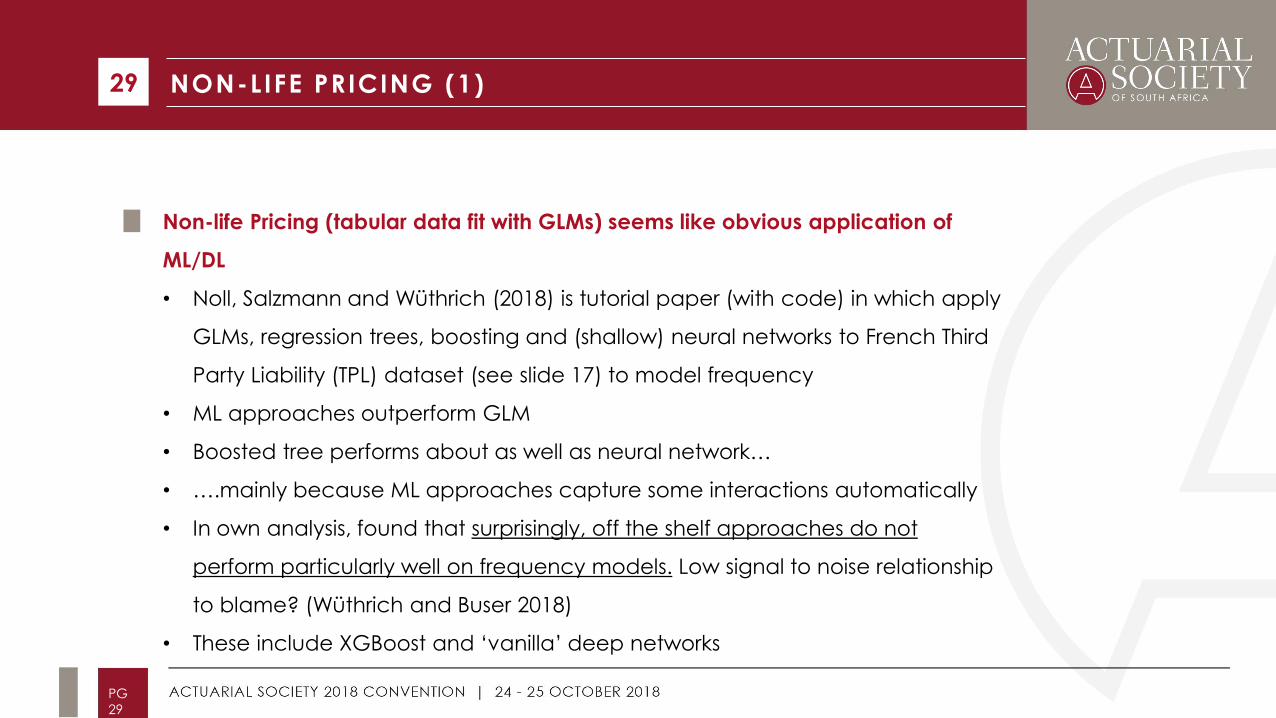
Non-life Pricing (tabular data fit with GLMs) seems like obvious application of
ML/DL
• Noll, Salzmann and Wüthrich (2018) is tutorial paper (with code) in which apply
GLMs, regression trees, boosting and (shallow) neural networks to French Third
Party Liability (TPL) dataset (see slide 17) to model frequency
• ML approaches outperform GLM
• Boosted tree performs about as well as neural network…
• ….mainly because ML approaches capture some interactions automatically
• In own analysis, found that surprisingly, off the shelf approaches do not
perform particularly well on frequency models. Low signal to noise relationship
to blame? (Wüthrich and Buser 2018)
• These include XGBoost and ‘vanilla’ deep networks
29
PG
29
NON-LIFE PRICING (2) 30
PG
30
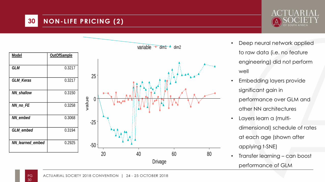
• Deep neural network applied
to raw data (i.e. no feature
engineering) did not perform
well
• Embedding layers provide
significant gain in
performance over GLM and
other NN architectures
• Layers learn a (multi-
dimensional) schedule of rates
at each age (shown after
applying t-SNE)
• Transfer learning – can boost
performance of GLM
-50
-25
0
25
20 40 60 80
Drivage
va
lue
variable dim1 dim2
Model OutOfSample
GLM 0.3217
GLM_Keras 0.3217
NN_shallow 0.3150
NN_no_FE 0.3258
NN_embed 0.3068
GLM_embed 0.3194
NN_learned_embed 0.2925
NON-LIFE PRICING (3) 31
PG
31
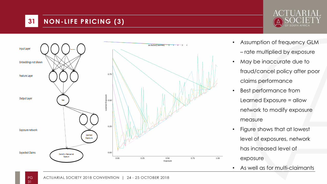
• Assumption of frequency GLM
– rate multiplied by exposure
• May be inaccurate due to
fraud/cancel policy after poor
claims performance
• Best performance from
Learned Exposure = allow
network to modify exposure
measure
• Figure shows that at lowest
level of exposures, network
has increased level of
exposure
• As well as for multi-claimants
0.00
0.25
0.50
0.75
0.00 0.25 0.50 0.75 1.00
Exposure
Le
arn
ed
Exp
osu
re
as.factor(ClaimNb) 0 1 2 3 4
IBNR RESERVING
IBNR Reserving boils down to regression of future reported claim amounts on past => good potential for
ML/DL approaches
• Granular reserving for claim type/property damaged/region/age etc difficult with normal chain-
ladder approach as too much data to derive LDFs judgementally (hopefully would not be done
mechanically unless lots of simple and clean data)
• Wüthrich (2018b) (who provides code + data) extends chain-ladder as a regression model to
incorporate features into derivation of LDF
• Method produces accurate aggregate and granular reserves
• DeepTriangle of Kuo (2018b) is less traditional approach. Joint prediction of Paid + Outstanding
claims using Recurrent Neural Networks and Embedding Layers
• Better performance than CL/GLM/Bayesian techniques on Schedule P data from USA
32
PG
32
jiji CXfC ,, ).(ˆ 1
TELEMATICS DATA (1)
Telematics produces high dimensional data (position, velocity, acceleration, road type, time of
day) at high frequencies – not immediately obvious how to incorporate into pricing
• Sophisticated approaches to analysing telematics data from outside actuarial literature using
recurrent neural networks plus embedding layers such as Dong, Li, Yao et al. (2016), Dong,
Yuan, Yang et al. (2017) and Wijnands, Thompson, Aschwanden et al. (2018)
• Within actuarial literature, series of papers by Wüthrich (2017), Gao and Wüthrich (2017) and
Gao, Meng and Wüthrich (2018) discuss analysis of velocity and acceleration information from
telematics data feed
• Focus on v-a heatmaps which capture velocity and acceleration profile of driver…
• … but these are also high dimensional
33
PG
33
TELEMATICS DATA (2) 34
PG
34
0.000
0.005
0.010
0.015
6 8 10 12 14 16 18 20
-2
-1
0
1
2
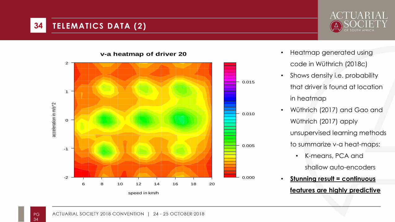
v-a heatmap of driver 20
speed in km/h
acce
lera
tion
in m
/s^2
• Heatmap generated using
code in Wüthrich (2018c)
• Shows density i.e. probability
that driver is found at location
in heatmap
• Wüthrich (2017) and Gao and
Wüthrich (2017) apply
unsupervised learning methods
to summarize v-a heat-maps:
• K-means, PCA and
shallow auto-encoders
• Stunning result = continuous
features are highly predictive
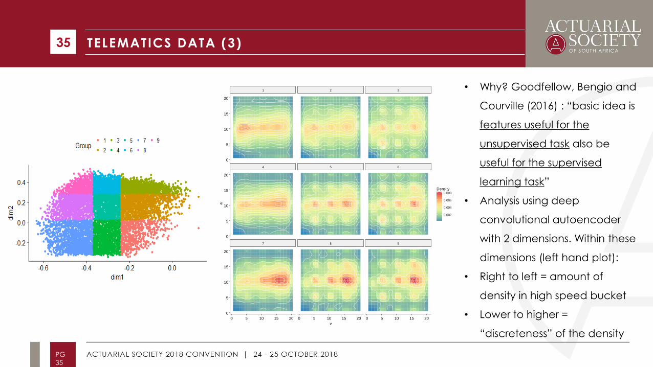
TELEMATICS DATA (3) 35
PG
35
• Why? Goodfellow, Bengio and
Courville (2016) : “basic idea is
features useful for the
unsupervised task also be
useful for the supervised
learning task”
• Analysis using deep
convolutional autoencoder
with 2 dimensions. Within these
dimensions (left hand plot):
• Right to left = amount of
density in high speed bucket
• Lower to higher =
“discreteness” of the density
7 8 9
4 5 6
1 2 3
0 5 10 15 20 0 5 10 15 20 0 5 10 15 20
0
5
10
15
20
0
5
10
15
20
0
5
10
15
20
v
a
0.002
0.004
0.006
0.008Density

AGENDA
1. Introduction
2. Background
• Machine Learning
• Deep Learning
• Five Main Deep Architectures
3. Applications in Actuarial Science
4. Discussion and Conclusion
36
PG
36

DISCUSSION
Conclusions to be drawn from the examples:
• Emphasis on predictive performance and potential gains of moving from traditional
actuarial and statistical methods to machine and deep learning approaches.
• Measurement framework utilized within machine learning – focus on testing predictive
performance.
• In wider deep learning context, focus on measurable improvements in predictive
performance led to refinements and enhancements of deep learning architectures
• Learned representations from deep neural networks often have readily interpretable
meaning
• Relies on data being available = role for CSI?
• Combination of deep learning plus traditional methods, refer to M4 Competition
37
PG
37
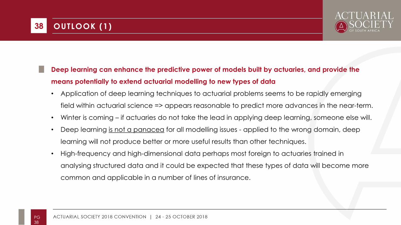
OUTLOOK (1)
Deep learning can enhance the predictive power of models built by actuaries, and provide the
means potentially to extend actuarial modelling to new types of data
• Application of deep learning techniques to actuarial problems seems to be rapidly emerging
field within actuarial science => appears reasonable to predict more advances in the near-term.
• Winter is coming – if actuaries do not take the lead in applying deep learning, someone else will.
• Deep learning is not a panacea for all modelling issues - applied to the wrong domain, deep
learning will not produce better or more useful results than other techniques.
• High-frequency and high-dimensional data perhaps most foreign to actuaries trained in
analysing structured data and it could be expected that these types of data will become more
common and applicable in a number of lines of insurance.
38
PG
38
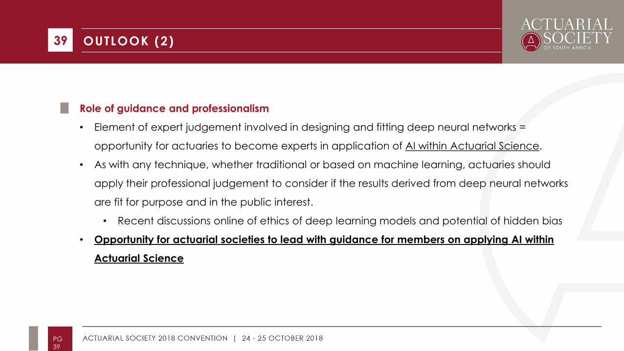
OUTLOOK (2)
Role of guidance and professionalism
• Element of expert judgement involved in designing and fitting deep neural networks =
opportunity for actuaries to become experts in application of AI within Actuarial Science.
• As with any technique, whether traditional or based on machine learning, actuaries should
apply their professional judgement to consider if the results derived from deep neural networks
are fit for purpose and in the public interest.
• Recent discussions online of ethics of deep learning models and potential of hidden bias
• Opportunity for actuarial societies to lead with guidance for members on applying AI within
Actuarial Science
39
PG
39
CONCLUSION 40
PG
40
Thank you for your attention. Any Questions?
Contact: [email protected]
Code: https://github.com/RonRichman/AI_in_Actuarial_Science
Blog: http://ronaldrichman.co.za/2018/07/25/thoughts-on-writing-ai-in-actuarial-science
REFERENCES
Bengio, Y. 2009. "Learning deep architectures for AI", Foundations and trends® in Machine Learning 2(1):1-127.
Breiman, L. 2001. "Statistical modeling: The two cultures (with comments and a rejoinder by the author)", Statistical Science 16(3):199-231.
De Brébisson, A., É. Simon, A. Auvolat, P. Vincent et al. 2015. "Artificial neural networks applied to taxi destination prediction", arXiv arXiv:1508.00021
Friedman, J., T. Hastie and R. Tibshirani. 2009. The Elements of Statistical Learning : Data Mining, Inference, and Prediction. New York: Springer-Verlag. http://dx.doi.org/10.1007/978-0-387-84858-7.
Gabrielli, A. and M. Wüthrich. 2018. "An Individual Claims History Simulation Machine", Risks 6(2):29.
Gao, G., S. Meng and M. Wüthrich. 2018. Claims Frequency Modeling Using Telematics Car Driving Data. SSRN. https://papers.ssrn.com/sol3/papers.cfm?abstract_id=3102371. Accessed: 29 June 2018.
Gao, G. and M. Wüthrich. 2017. Feature Extraction from Telematics Car Driving Heatmaps. SSRN. https://papers.ssrn.com/sol3/papers.cfm?abstract_id=3070069. Accessed: June 29 2018.
Goodfellow, I., Y. Bengio and A. Courville. 2016. Deep Learning. MIT Press.
Guo, C. and F. Berkhahn. 2016. "Entity embeddings of categorical variables", arXiv arXiv:1604.06737
Hainaut, D. 2018. "A neural-network analyzer for mortality forecast", Astin Bulletin 48(2):481-508.
Hannun, A., C. Case, J. Casper, B. Catanzaro et al. 2014. "Deep speech: Scaling up end-to-end speech recognition", arXiv arXiv:1412.5567
Hejazi, S. and K. Jackson. 2016. "A neural network approach to efficient valuation of large portfolios of variable annuities", Insurance: Mathematics and Economics 70:169-181.
Krizhevsky, A., I. Sutskever and G. Hinton. 2012. "Imagenet classification with deep convolutional neural networks," Paper presented at Advances in Neural Information Processing Systems. 1097-1105.
Kuo, K. 2018. "DeepTriangle: A Deep Learning Approach to Loss Reserving", arXiv arXiv:1804.09253
Makridakis, S., E. Spiliotis and V. Assimakopoulos. 2018. "The M4 Competition: Results, findings, conclusion and way forward", International Journal of Forecasting
Mitchell, T. 1997. Machine learning. McGraw-Hill Boston, MA.
Noll, A., R. Salzmann and M. Wüthrich. 2018. Case Study: French Motor Third-Party Liability Claims. SSRN. https://ssrn.com/abstract=3164764 Accessed: 17 June 2018.
Schreiber, D. 2017. The Future of Insurance. DIA Munich 2017: https://www.youtube.com/watch?time_continue=1&v=LDOhFHJqKqI. Accessed: 17 June 2018.
Shmueli, G. 2010. "To explain or to predict?", Statistical Science:289-310.
Smith, M., F. Beyers and J. De Villiers. 2016. "A method of parameterising a feed forward multi-layered perceptron artificial neural network, with reference to South African financial markets", South African Actuarial Journal 16(1):35-
67.
Sutton, R. and A. Barto. 2018. Reinforcement learning: An introduction, Second Edition. MIT Press.
Szegedy, C., W. Liu, Y. Jia, P. Sermanet et al. "Going deeper with convolutions," Paper presented at.
Wu, Y., M. Schuster, Z. Chen, Q. Le et al. 2016. "Google's neural machine translation system: Bridging the gap between human and machine translation", arXiv arXiv:1609.08144
Wüthrich, M. 2018a. Neural networks applied to chain-ladder reserving. SSRN. https://papers.ssrn.com/sol3/papers.cfm?abstract_id=2966126. Accessed: 1 July 2018.
Wüthrich, M. 2018b. v-a Heatmap Simulation Machine. https://people.math.ethz.ch/~wueth/simulation.html. Accessed: 1 July 2018.
Wüthrich, M. and C. Buser. 2018. Data analytics for non-life insurance pricing. Swiss Finance Institute Research Paper. https://ssrn.com/abstract=2870308. Accessed: 17 June 2018.
Wüthrich, M.V. 2017. "Covariate selection from telematics car driving data", European Actuarial Journal 7(1):89-108.
41
PG
41