Embed Size (px)
Citation preview
BS4aActuarial Science I
George DeligiannidisDepartment of Statistics
University of Oxford
MT 2015
BS4aActuarial Science I
16 lectures MT 2014
Aims
This unit is supported by the Institute of Actuaries. It has been designed to give the under-graduate mathematician an introduction to the financial and insurance worlds in which thepractising actuary works. Students will cover the basic concepts of discounted cash-flows andapplications.
In the examination, a student obtaining at least an upper second class mark on the wholeunit BS4/OBS4 can expect to gain exemption from the Institute of Actuaries’ paper CT1, whichis a compulsory paper in their cycle of professional actuarial examinations. An IndependentExaminer approved by the Institute of Actuaries will inspect examination papers and scriptsand may adjust the pass requirements for exemptions.
Synopsis
Fundamental nature of actuarial work. Use of cash-flow models to describe financial transac-tions. Time value of money using the concepts of compound interest and discounting.
Interest rate models. Present values and the accumulated values of a stream of equal orunequal payments using specified rates of interest. Interest rates in terms of different timeperiods. Equation of value, rate of return of a cash-flow, existence criteria.
Loan repayment schemes. Investment project appraisal, funds and weighted rates of return.Inflation modelling, inflation indices, real rates of return, inflation adjustments. Valuation offixed-interest securities, taxation and index-linked bonds.
Price and value of forward contracts. Term structure of interest rates, spot rates, forwardrates and yield curves. Duration, convexity and immunisation. Simple stochastic interest ratemodels. Investment and risk characteristics of investments.
Reading
All of the following are available from the Publications Unit, Institute of Actuaries, 4 WorcesterStreet, Oxford OX1 2AW
• Subject CT1 [102]: Financial Mathematics Core reading. Faculty & Institute of Actuaries
• J. J. McCutcheon and W. F. Scott: An Introduction to the Mathematics of Finance.Heinemann (1986)
• P. Zima and R. P. Brown: Mathematics of Finance. McGraw-Hill Ryerson (1993)
• N. L. Bowers et al, Actuarial mathematics, 2nd edition, Society of Actuaries (1997)
• J. Danthine and J. Donaldson: Intermediate Financial Theory. 2nd edition, AcademicPress Advanced Finance (2005)

Contents iii
Notes
These notes have been assembled from earlier notes produced by Matthias Winkel and DanielClarke.
Contents
1 Introduction 11.1 The actuarial profession . . . . . . . . . . . . . . . . . . . . . . . . . . . . . . . . 11.2 The generalised cash-flow model . . . . . . . . . . . . . . . . . . . . . . . . . . . 21.3 Examples and course overview . . . . . . . . . . . . . . . . . . . . . . . . . . . . 3
2 The theory of compound interest 52.1 Simple versus compound interest . . . . . . . . . . . . . . . . . . . . . . . . . . . 52.2 Nominal and effective rates . . . . . . . . . . . . . . . . . . . . . . . . . . . . . . 72.3 Discount factors and discount rates . . . . . . . . . . . . . . . . . . . . . . . . . . 8
3 Valuing cash-flows 93.1 Accumulating and discounting in the constant-i model . . . . . . . . . . . . . . . 93.2 Time-dependent interest rates . . . . . . . . . . . . . . . . . . . . . . . . . . . . . 93.3 Accumulation factors . . . . . . . . . . . . . . . . . . . . . . . . . . . . . . . . . . 103.4 Time value of money . . . . . . . . . . . . . . . . . . . . . . . . . . . . . . . . . . 113.5 Continuous cash-flows . . . . . . . . . . . . . . . . . . . . . . . . . . . . . . . . . 123.6 Example: withdrawal of interest as a cash-flow . . . . . . . . . . . . . . . . . . . 12
4 The yield of a cash-flow 134.1 Definition of the yield of a cash-flow . . . . . . . . . . . . . . . . . . . . . . . . . 134.2 General results ensuring the existence of yields . . . . . . . . . . . . . . . . . . . 144.3 Example: APR of a loan . . . . . . . . . . . . . . . . . . . . . . . . . . . . . . . . 154.4 Numerical calculation of yields . . . . . . . . . . . . . . . . . . . . . . . . . . . . 16
5 Annuities and fixed-interest securities 175.1 Annuity symbols . . . . . . . . . . . . . . . . . . . . . . . . . . . . . . . . . . . . 175.2 Fixed-interest securities . . . . . . . . . . . . . . . . . . . . . . . . . . . . . . . . 19
6 Mortgages and loans 216.1 Loan repayment schemes . . . . . . . . . . . . . . . . . . . . . . . . . . . . . . . . 216.2 Loan outstanding, interest/capital components . . . . . . . . . . . . . . . . . . . 226.3 Fixed, capped and discount mortgages . . . . . . . . . . . . . . . . . . . . . . . . 236.4 Comparison of mortgages . . . . . . . . . . . . . . . . . . . . . . . . . . . . . . . 24
iv
Contents v
7 Funds and weighted rates of return 257.1 Money-weighted rate of return . . . . . . . . . . . . . . . . . . . . . . . . . . . . 257.2 Time-weighted rate of return . . . . . . . . . . . . . . . . . . . . . . . . . . . . . 267.3 Units in investment funds . . . . . . . . . . . . . . . . . . . . . . . . . . . . . . . 267.4 Fees . . . . . . . . . . . . . . . . . . . . . . . . . . . . . . . . . . . . . . . . . . . 287.5 Fund types . . . . . . . . . . . . . . . . . . . . . . . . . . . . . . . . . . . . . . . 28
8 Inflation 298.1 Inflation indices . . . . . . . . . . . . . . . . . . . . . . . . . . . . . . . . . . . . . 298.2 Modelling inflation . . . . . . . . . . . . . . . . . . . . . . . . . . . . . . . . . . . 308.3 Constant inflation rate . . . . . . . . . . . . . . . . . . . . . . . . . . . . . . . . . 318.4 Index-linking . . . . . . . . . . . . . . . . . . . . . . . . . . . . . . . . . . . . . . 32
9 Taxation 339.1 Fixed-interest securities and running yields . . . . . . . . . . . . . . . . . . . . . 339.2 Income tax and capital gains tax . . . . . . . . . . . . . . . . . . . . . . . . . . . 349.3 Offsetting . . . . . . . . . . . . . . . . . . . . . . . . . . . . . . . . . . . . . . . . 359.4 Indexation of CGT . . . . . . . . . . . . . . . . . . . . . . . . . . . . . . . . . . . 359.5 Inflation adjustments . . . . . . . . . . . . . . . . . . . . . . . . . . . . . . . . . . 35
10 Project appraisal 3710.1 Net cash-flows and a first example . . . . . . . . . . . . . . . . . . . . . . . . . . 3710.2 Payback periods and a second example . . . . . . . . . . . . . . . . . . . . . . . . 3810.3 Profitability, comparison and cross-over rates . . . . . . . . . . . . . . . . . . . . 3910.4 Reasons for different yields/profitability curves . . . . . . . . . . . . . . . . . . . 40
11 Modelling future lifetimes 4111.1 Introduction to life insurance . . . . . . . . . . . . . . . . . . . . . . . . . . . . . 4111.2 Valuation under uncertainty . . . . . . . . . . . . . . . . . . . . . . . . . . . . . . 42
11.2.1 Examples . . . . . . . . . . . . . . . . . . . . . . . . . . . . . . . . . . . . 4211.2.2 Uncertain payment . . . . . . . . . . . . . . . . . . . . . . . . . . . . . . . 43
11.3 Pricing of corporate bonds . . . . . . . . . . . . . . . . . . . . . . . . . . . . . . . 4311.4 Expected yield . . . . . . . . . . . . . . . . . . . . . . . . . . . . . . . . . . . . . 4611.5 Lives aged x . . . . . . . . . . . . . . . . . . . . . . . . . . . . . . . . . . . . . . . 4711.6 Curtate lifetimes . . . . . . . . . . . . . . . . . . . . . . . . . . . . . . . . . . . . 4811.7 Examples . . . . . . . . . . . . . . . . . . . . . . . . . . . . . . . . . . . . . . . . 49
12 Lifetime distributions and life-tables 5012.1 Actuarial notation for life products. . . . . . . . . . . . . . . . . . . . . . . . . . 5012.2 Simple laws of mortality . . . . . . . . . . . . . . . . . . . . . . . . . . . . . . . . 5112.3 The life-table . . . . . . . . . . . . . . . . . . . . . . . . . . . . . . . . . . . . . . 5112.4 Example . . . . . . . . . . . . . . . . . . . . . . . . . . . . . . . . . . . . . . . . . 52
13 Select life-tables and applications 5413.1 Select life-tables . . . . . . . . . . . . . . . . . . . . . . . . . . . . . . . . . . . . 5413.2 Multiple premiums . . . . . . . . . . . . . . . . . . . . . . . . . . . . . . . . . . . 5513.3 Interpolation for non-integer ages x+ u, x ∈ N, u ∈ (0, 1) . . . . . . . . . . . . . 5613.4 Practical concerns . . . . . . . . . . . . . . . . . . . . . . . . . . . . . . . . . . . 57
Contents vi
14 Evaluation of life insurance products 5814.1 Life assurances . . . . . . . . . . . . . . . . . . . . . . . . . . . . . . . . . . . . . 5814.2 Life annuities and premium conversion relations . . . . . . . . . . . . . . . . . . . 5914.3 Continuous life assurance and annuity functions . . . . . . . . . . . . . . . . . . . 6014.4 More general types of life insurance . . . . . . . . . . . . . . . . . . . . . . . . . . 60
15 Premiums 6215.1 Different types of premiums . . . . . . . . . . . . . . . . . . . . . . . . . . . . . . 6215.2 Net premiums . . . . . . . . . . . . . . . . . . . . . . . . . . . . . . . . . . . . . . 6315.3 Office premiums . . . . . . . . . . . . . . . . . . . . . . . . . . . . . . . . . . . . 6315.4 Prospective policy values . . . . . . . . . . . . . . . . . . . . . . . . . . . . . . . . 64
16 Reserves 6616.1 Reserves and random policy values . . . . . . . . . . . . . . . . . . . . . . . . . . 6616.2 Thiele’s differential equation . . . . . . . . . . . . . . . . . . . . . . . . . . . . . . 68
A 70A.1 Some old exam questions . . . . . . . . . . . . . . . . . . . . . . . . . . . . . . . 70
B Notation and introduction to probability 72

Lecture 1
Introduction
Reading: CT1 Core Reading Unit 1Further reading: http://www.actuaries.org.uk
After some general information about relevant history and about the work of an actuary, weintroduce cash-flow models as the basis of this course and as a suitable framework to describeand look beyond the contents of this course.
1.1 The actuarial profession
Actuarial Science is a discipline with its own history. The Institute of Actuaries was formed in1848, (the Faculty of Actuaries in Scotland in 1856, the two merged in 2010), but the roots goback further. An important event was the construction of the first life table by Sir EdmundHalley in 1693. However, Actuarial Science is not oldfashioned. The language of probabilitytheory was gradually adopted as it developed in the 20th century; computing power and newcommunication technologies have changed the work of actuaries. The growing importance andcomplexity of financial markets continues to fuel actuarial work; current debates and changesin life expentancy, retirement age, viability of pension schemes are core actuarial topics thatthe profession vigorously embraces.
Essentially, the job of an actuary is risk assessment. Traditionally, this was insurance risk,life insurance, later general insurance (health, home, property etc). As typically large amountsof money, reserves, have to be maintained, this naturally extended to investment strategiesincluding the assessment of risk in financial markets. Today, the Actuarial Profession claimsyet more broadly to make “financial sense of the future”.
To become a Fellow of the Institute/Faculty of Actuaries in the UK, an actuarial trainee hasto pass nine mathematics, statistics, economics and finance examinations (core technical series –CT), examinations on risk management, reporting and communication skills (core applications –CA), and three specialist examinations in the chosen areas of specialisation (specialist technicaland specialist applications series – ST and SA) and for a UK fellowship an examination onUK specifics. This programme takes normally at least three or four years after a mathematicaluniversity degree and while working for an insurance company under the guidance of a Fellowof the Institute/Faculty of Actuaries.
This lecture course is an introductory course where important foundations are laid and anoverview of further actuarial education and practice is given. An upper second mark in theexamination following the full OBS4/BS4 unit normally entitles to an exemption from the CT1
1

Lecture Notes – BS4a Actuarial Science – Oxford MT 2015 2
paper. The CT3 paper is covered by the Part A Probability and Statistics courses. A furtherexemption, from CT4, is available for BS3 Stochastic Modelling.
1.2 The generalised cash-flow model
The cash-flow model systematically captures payments either between different parties or, aswe shall focus on, in an inflow/outflow way from the perspective of one party. This can be doneat different levels of detail, depending on the purpose of an investigation, the complexity of thesituation, the availability of reliable data etc.
Example 1 Look at the transactions on a bank statement for September 2011.
Date Description Money out Money in
01-09-11 Gas-Elec-Bill £21.3704-09-11 Withdrawal £100.0015-09-11 Telephone-Bill £14.7216-09-11 Mortgage Payment £396.1228-09-11 Withdrawal £150.0030-09-11 Salary £1,022.54
Extracting the mathematical structure of this example we define elementary cash-flows.
Definition 2 A cash-flow is a vector (tj , cj)1≤j≤m of times tj ∈ R and amounts cj ∈ R. Positiveamounts cj > 0 are called inflows. If cj < 0, then |cj | is called an outflow.
Example 3 The cash-flow of Example 80 is mathematically given by
j tj cj1 1 −21.372 4 −100.003 15 −14.72
j tj cj4 16 −396.125 28 −150.006 30 1,022.54
Often, the situation is not as clear as this, and there may be uncertainty about the time/amountof a payment. This can be modelled stochastically.
Definition 4 A random cash-flow is a random vector (Tj , Cj)1≤j≤M of times Tj ∈ R andamounts Cj ∈ R with a possibly random length M ∈ N.
Sometimes, in fact always in this course, the random structure is simple and the times or theamounts are deterministic, or even the only randomness is that a well specified payment mayfail to happen with a certain probability.
Lecture Notes – BS4a Actuarial Science – Oxford MT 2015 3
Example 5 Future transactions on a bank account (say for November 2011)
j Tj Cj Description
1 1 −21.37 Gas-Elec-Bill2 T2 C2 Withdrawal?3 15 C3 Telephone-Bill
j Tj Cj Description
4 16 −396.12 Mortgage payment5 T5 C5 Withdrawal?6 30 1,022.54 Salary
Here we assume a fixed Gas-Elec-Bill but a varying telephone bill. Mortgage payment andsalary are certain. Any withdrawals may take place. For a full specification of the randomcash-flow we would have to give the (joint!) laws of the random variables.
This example shows that simple situations are not always easy to model. It is an importantpart of an actuary’s work to simplify reality into tractable models. Sometimes, it is worthdropping or generalising the time specification and just list approximate or qualitative (’big’,’small’, etc.) amounts of income and outgo. cash-flows can be represented in various ways asthe following important examples illustrate.
1.3 Examples and course overview
Example 6 (Zero-coupon bond) Usually short-term investments with interest paid at theend of the term, e.g. invest £99 for ninety days for a payoff of £100.
j tj cj1 0 −992 90 100
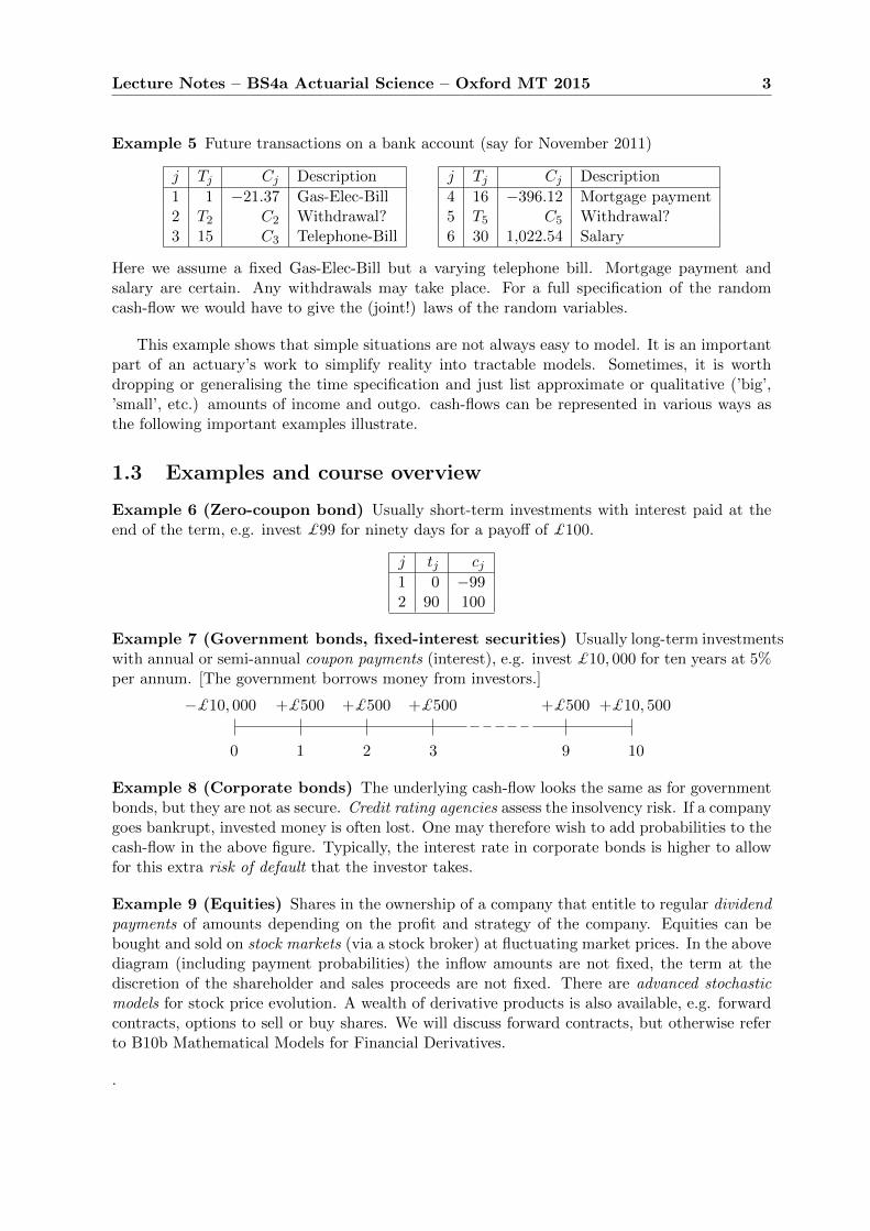
Example 7 (Government bonds, fixed-interest securities) Usually long-term investmentswith annual or semi-annual coupon payments (interest), e.g. invest £10, 000 for ten years at 5%per annum. [The government borrows money from investors.]
−£10, 000 +£500 +£500 +£500 +£500 +£10, 500
0 1 2 3 9 10
Example 8 (Corporate bonds) The underlying cash-flow looks the same as for governmentbonds, but they are not as secure. Credit rating agencies assess the insolvency risk. If a companygoes bankrupt, invested money is often lost. One may therefore wish to add probabilities to thecash-flow in the above figure. Typically, the interest rate in corporate bonds is higher to allowfor this extra risk of default that the investor takes.
Example 9 (Equities) Shares in the ownership of a company that entitle to regular dividendpayments of amounts depending on the profit and strategy of the company. Equities can bebought and sold on stock markets (via a stock broker) at fluctuating market prices. In the abovediagram (including payment probabilities) the inflow amounts are not fixed, the term at thediscretion of the shareholder and sales proceeds are not fixed. There are advanced stochasticmodels for stock price evolution. A wealth of derivative products is also available, e.g. forwardcontracts, options to sell or buy shares. We will discuss forward contracts, but otherwise referto B10b Mathematical Models for Financial Derivatives.
.
Lecture Notes – BS4a Actuarial Science – Oxford MT 2015 4
Example 10 (Index-linked securities) Inflation-adjusted securities: coupons and redemp-tion payment increase in line with inflation, by tracking an inflation index.
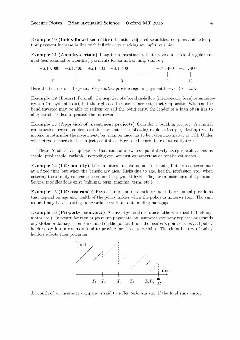
Example 11 (Annuity-certain) Long term investments that provide a series of regular an-nual (semi-annual or monthly) payments for an initial lump sum, e.g.
−£10, 000 +£1, 400 +£1, 400 +£1, 400 +£1, 400 +£1, 400
0 1 2 3 9 10
Here the term is n = 10 years. Perpetuities provide regular payment forever (n =∞).
Example 12 (Loans) Formally the negative of a bond cash-flow (interest-only loan) or annuity-certain (repayment loan), but the rights of the parties are not exactly opposite. Whereas thebond investor may be able to redeem or sell the bond early, the lender of a loan often has toobey stricter rules, to protect the borrower.
Example 13 (Appraisal of investment projects) Consider a building project. An initialconstruction period requires certain payments, the following exploitation (e.g. letting) yieldsincome in return for the investment, but maintenance has to be taken into accout as well. Underwhat circumstances is the project profitable? How reliable are the estimated figures?
These “qualitative” questions, that can be answered qualitatively using specifications asstable, predictable, variable, increasing etc. are just as important as precise estimates.
Example 14 (Life annuity) Life annuities are like annuities-certain, but do not terminateat a fixed time but when the beneficiary dies. Risks due to age, health, profession etc. whenentering the annuity contract determine the payment level. They are a basic form of a pension.Several modifications exist (minimal term, maximal term, etc.).
Example 15 (Life assurance) Pays a lump sum on death for monthly or annual premiumsthat depend on age and health of the policy holder when the policy is underwritten. The sumassured may be decreasing in accordance with an outstanding mortgage.
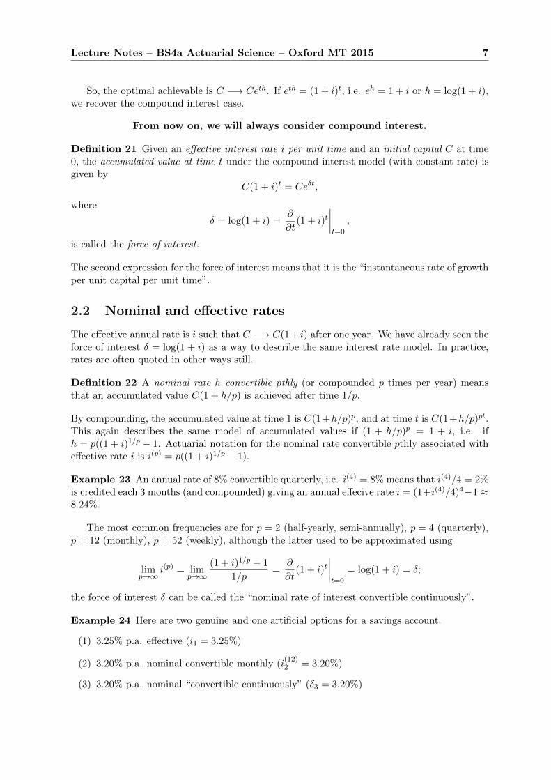
Example 16 (Property insurance) A class of general insurance (others are health, building,motor etc.). In return for regular premium payments, an insurance company replaces or refundsany stolen or damaged items included on the policy. From the insurer’s point of view, all policyholders pay into a common fund to provide for those who claim. The claim history of policyholders affects their premium.
-time
6fund
�����
T1
���
T2
����
T3
����
T4
����
T5
��
T6
��
R
uA branch of an insurance company is said to suffer technical ruin if the fund runs empty.

Lecture 2
The theory of compound interest
Reading: CT1 Core Reading Units 2-3, McCutcheon-Scott Chapter 1, Sections 2.1-2.4
Quite a few problems that we deal with in this course can be approached in an intuitive way.However, the mathematical and more powerful approach to problem solving is to set up amathematical model in which the problem can be formalised and generalised. The concept ofcash-flows seen in the last lecture is one part of such a model. In this lecture, we shall constructanother part, the compound interest model in which interest on capital investments, loans etc.can be computed. This model will play a crucial role throughout the course.
In any mathematical model, reality is only partially represented. An important part ofmathematical modelling is the discussion of model assumptions and the interpretation of theresults of the model.
2.1 Simple versus compound interest
We are familiar with the concept of interest in everyday banking: the bank pays interest onpositive balances on current accounts and savings accounts (not much, but some), and it chargesinterest on loans and overdrawn current accounts. Reasons for this include that
• people/institutions borrowing money are willing to pay a fee (in the future) for the useof this money now,
• there is price inflation in that £100 lose purchasing power between the beginning and theend of a loan as prices increase,
• there is often a risk that the borrower may not be able to repay the loan.
To develop a mathematical framework, consider an “interest rate h” per unit time, under whichan investment of C at time 0 will receive interest Ch by time 1, giving total value C(1 + h):
C −→ C(1 + h),
e.g. for h = 4% we get C −→ 1.04C.There are two natural ways to extend this to general times t:
Definition 17 (Simple interest) Invest C, receive C(1 + th) after t years. The simple in-terest on C at rate h for time t is Cth.
5

Lecture Notes – BS4a Actuarial Science – Oxford MT 2015 6
Definition 18 (Compound interest) Invest C, receive C(1 + i)t after t years. The com-pound interest on C at rate i for time t is C((1 + i)t − 1).
For integer t = n, this is as if a bank balance was updated at the end of each year
C −→ C(1 + i) −→ (C(1 + i))(1 + i) = C(1 + i)2 −→ (C(1 + i)n−1)(1 + i) = C(1 + i)n.
Example 19 Given an interest rate of i = 6% per annum (p.a.), investing C = £1, 000 fort = 2 years yields
Isimp = C2i = £120.00 and Icomp = C((1 + i)2 − 1
)= C(2i+ i2) = £123.60,
where we can interpret Ci2 as interest on interest, i.e. interest for the second year paid at ratei on the interet Ci for the first year.
Compound interest behaves well under term-splitting: for t = s+ r
C −→ C(1 + i)s −→ (C(1 + i)s) (1 + i)r = C(1 + i)t,
i.e. investing C at rate i first for s years and then the resulting C(1 + i)s for a further r yearsgives the same as directly investing C for t = s+ r years. Under simple interest
C −→ C(1 + hs) −→ C(1 + hs)(1 + hr) = C(1 + ht+ srh2) > C(1 + ht),
(in the case C > 0, r > 0, s > 0). The difference Csrh2 = (Chs)hr is interest on the interestChs that was already paid at time s for the first s years.
What is the best we can achieve by term-splitting under simple interest?
Denote by St(C) = C(1 + th) the accumulated value under simple interest at rate h for time t.We have seen that Sr ◦ Ss(C) > Sr+s(C).
Proposition 20 Fix t > 0 and h. Then
supn∈N,r1,...,rn∈R+:r1+···+rn=t
Srn ◦ Srn−1 ◦ · · · ◦ Sr1(C) = limn→∞
St/n ◦ · · · ◦ St/n(C) = ethC.
Proof: For the second equality we first note that
St/n ◦ · · · ◦ St/n(C) =
(1 +
t
nh
)nC → ethC,
becauselog((1 + th/n)n) = n log(1 + th/n) = n(th/n+O(1/n2))→ th.
For the first equality,
erh = 1 + rh+r2h2
2+ · · · ≥ 1 + rh
so if r1 + · · ·+ rn = t, then
ethC = er1her2h · · · ernhC ≥ (1 + r1h)(1 + r2h) · · · (1 + rnh)C = Srn ◦ Srn−1 ◦ · · · ◦ Sr1(C).
2
Lecture Notes – BS4a Actuarial Science – Oxford MT 2015 7
So, the optimal achievable is C −→ Ceth. If eth = (1 + i)t, i.e. eh = 1 + i or h = log(1 + i),we recover the compound interest case.
From now on, we will always consider compound interest.
Definition 21 Given an effective interest rate i per unit time and an initial capital C at time0, the accumulated value at time t under the compound interest model (with constant rate) isgiven by
C(1 + i)t = Ceδt,
where
δ = log(1 + i) =∂
∂t(1 + i)t
∣∣∣∣t=0
,
is called the force of interest.
The second expression for the force of interest means that it is the “instantaneous rate of growthper unit capital per unit time”.
2.2 Nominal and effective rates
The effective annual rate is i such that C −→ C(1 + i) after one year. We have already seen theforce of interest δ = log(1 + i) as a way to describe the same interest rate model. In practice,rates are often quoted in other ways still.
Definition 22 A nominal rate h convertible pthly (or compounded p times per year) meansthat an accumulated value C(1 + h/p) is achieved after time 1/p.
By compounding, the accumulated value at time 1 is C(1+h/p)p, and at time t is C(1+h/p)pt.This again describes the same model of accumulated values if (1 + h/p)p = 1 + i, i.e. ifh = p((1 + i)1/p − 1. Actuarial notation for the nominal rate convertible pthly associated witheffective rate i is i(p) = p((1 + i)1/p − 1).
Example 23 An annual rate of 8% convertible quarterly, i.e. i(4) = 8% means that i(4)/4 = 2%is credited each 3 months (and compounded) giving an annual effecive rate i = (1+i(4)/4)4−1 ≈8.24%.
The most common frequencies are for p = 2 (half-yearly, semi-annually), p = 4 (quarterly),p = 12 (monthly), p = 52 (weekly), although the latter used to be approximated using
limp→∞
i(p) = limp→∞
(1 + i)1/p − 1
1/p=
∂
∂t(1 + i)t
∣∣∣∣t=0
= log(1 + i) = δ;
the force of interest δ can be called the “nominal rate of interest convertible continuously”.
Example 24 Here are two genuine and one artificial options for a savings account.
(1) 3.25% p.a. effective (i1 = 3.25%)
(2) 3.20% p.a. nominal convertible monthly (i(12)2 = 3.20%)
(3) 3.20% p.a. nominal “convertible continuously” (δ3 = 3.20%)
Lecture Notes – BS4a Actuarial Science – Oxford MT 2015 8
After one year, an initial capital of £10,000 accumulates to
(1) 10, 000× (1 + 3.25%) = 10, 325.00 = R1,
(2) 10, 000× (1 + 3.20%/12)12 = 10, 324.74 = R2,
(3) 10, 000× e3.20% = 10, 325.18 = R3.
Although interest may be credited to the account differently, an investment into (j) just consistsof deposit and withdrawal, so the associated cash-flow is ((0,−10000), (1, Rj)), and we can useRj to decide between the options. We can also compare i2 ≈ 3.2474% and i3 ≈ 3.2518% orcalculate δ1 and δ2 to compare with δ3 etc.
Interest rates always refer to some time unit. The standard choice is one year, but itsometimes eases calculations to choose six months, one month or one day. All definitions wehave made reflect the assumption that the interest rate does not vary with the initial capital Cnor with the term t. We refer to this model of accumulated values as the constant-i model, orthe constant-δ model.
2.3 Discount factors and discount rates
Before we more fully apply the constant-i model to cash-flows in Lecture 3, let us discuss thenotion of discount. We are used to discounts when shopping, usually a percentage reduction inprice, time being implicit. Actuaries use the notion of an effective rate of discount d per timeunit to represent a reduction of C to C(1− d) if payment takes place a time unit early.
This is consistent with the constant-i model, if the payment of C(1 − d) accumulates toC = (C(1− d))(1 + i) after one time unit, i.e. if
(1− d)(1 + i) = 1 ⇐⇒ d = 1− 1
1 + i.
A more prominent role will be played by the discount factor v = 1 − d, which answers thequestion
How much will we have to invest now to have 1 at time 1?
Definition 25 In the constant-i model, we refer to v = 1/(1 + i) as the associated discountfactor and to d = 1− v as the associated effective annual rate of discount.
Example 26 How much do we have to invest now to have 1 at time t? If we invest C, thisaccumulates to C(1 + i)t after t years, hence we have to invest C = 1/(1 + i)t = vt.
Lecture 3
Valuing cash-flows
Reading: CT1 Core Reading Units 3 and 5, McCutcheon-Scott Chapter 2
In Lecture 2 we set up the constant-i interest rate model and saw how a past deposit accumulatesand a future payment can be discounted. In this lecture, we combine these concepts with thecash-flow model of Lecture 1 by assigning time-t values to cash-flows. We also introduce general(deterministic) time-dependent interest models, and continuous cash-flows that model manysmall payments as infinitesimal payment streams.
3.1 Accumulating and discounting in the constant-i model
Given a cash-flow c = (cj , tj)1≤j≤m of payments cj at time tj and a time t with t ≥ tj for all j,we can write the joint accumulated value of all payments by time t according to the constant-imodel as
AValt(c) =
m∑j=1
cj(1 + i)t−tj =
m∑j=1
cjeδ(t−tj),
because each payment cj at time tj earns compound interest for t−tj time units. Note that somecj may be negative, so the accumulated value could become negative. We assume implicitlythat the same interest rate applies to positive and negative balances.
Similarly, given a cash-flow c = (cj , tj)1≤j≤m of payments cj at time tj and a time t < tj forall j, we can write the joint discounted value at time t of all payments as
DValt(c) =
m∑j=1
cjvtj−t =
m∑j=1
cj(1 + i)−(tj−t) =
m∑j=1
cje−δ(tj−t).
This discounted value is the amount we invest at time t to be able to spend cj at time tj for allj.
3.2 Time-dependent interest rates
So far, we have assumed that interest rates are constant over time. Suppose, we now let i = i(k)vary with time k ∈ N. We define the accumulated value at time n for an investment of C attime 0 as
C(1 + i(1))(1 + i(2)) · · · (1 + i(n− 1)) · · · (1 + i(n)).
9

Lecture Notes – BS4a Actuarial Science – Oxford MT 2015 10
Example 27 A savings account pays interest at i(1) = 2% in the first year and i(2) = 5% inthe second year, with interest from the first year reinvested. Then the account balance evolvesas 1, 000 −→ 1, 000(1 + i(1)) = 1, 020 −→ 1, 000(1 + i(1))(1 + i(2)) = 1, 071.
When varying interest rates between non-integer times, it is often nicer to specify the force ofinterest δ(t) which we saw to have a local meaning as the infinitesimal rate of capital growthunder compound interest:
C −→ C exp
(∫ t
0δ(s)ds
)= R(t).
Note that now (under some right-continuity assumptions)
∂
∂tR(t)
∣∣∣∣t=0
= R(0)δ(0) and more generally∂
∂tR(t) = δ(t)R(t),
so that the interpretation of δ(t) as local rate of capital growth at time t still applies.
Example 28 If δ(·) is piecewise constant, say constant δj on (tj−1, tj ], j = 1, . . . , n, then
C −→ Ceδ1r1eδ2r2 · · · eδnrn , where rj = tj − tj−1.
Definition 29 Given a time-dependent force of interest δ(t), t ∈ R+, we define the accumulatedvalue at time t ≥ 0 of an initial capital C ∈ R under a force of interest δ(·) as
R(t) = C exp
(∫ t
0δ(s)ds
).
Also, we may refer to I(t) = R(t)− C as the interest from time 0 to time t under δ(·).
3.3 Accumulation factors
Given a time-dependent interest model δ(·), let us define accumulation factors from s to t
A(s, t) = exp
(∫ t
sδ(r)dr
), s < t. (1)
Just as C −→ R(t) = CA(0, t) for an investment of C at time 0 for a term t, we use A(s, t) as afactor to turn an investment of C at time s into its accumulated value CA(s, t) at time t. Thisbehaves well under term-splitting, since
C −→ CA(0, s) −→ (CA(0, s))A(s, t)=C exp
(∫ s
0δ(r)dr
)exp
(∫ t
sδ(r)dr
)=CA(0, t).
More generally, note the consistency property A(r, s)A(s, t) = A(r, t), and conversely:
Proposition 30 Suppose, A : {(s, t) : s ≤ t} → (0,∞) satisfies the consistency property andt 7→ A(s, t) is differentiable for all s, then there is a function δ(·) such that (1) holds.
Lecture Notes – BS4a Actuarial Science – Oxford MT 2015 11
Proof: Since consistency for r = s = t implies A(t, t) = 1, we can define as (right-hand)derivative
δ(t) = limh↓0
A(t, t+ h)−A(t, t)
h= lim
h↓0
A(0, t+ h)−A(0, t)
hA(0, t),
where we also applied consistency. With g(t) = A(0, t) and f(t) = log(A(0, t))
δ(t) =g′(t)
g(t)= f ′(t) ⇒ log(A(0, t)) = f(t) =
∫ t
0δ(s)ds.
Since consistency implies A(s, t) = A(0, t)/A(0, s), we obtain (1). 2
We included the apparently unrealistic A(s, t) < 1 (accumulated value less than the initialcapital) that leads to negative δ(·). This can be useful for some applications where δ(·) is notpre-specified, but connected to investment performance where prices can go down as well asup, or to inflation/deflation. Similarly, we allow any i ∈ (−1,∞), so that the associated 1-yearaccumulation factor 1 + i is positive, but possibly less than 1.
3.4 Time value of money
We have discussed accumulated and discounted values in the constant-i model. In the time-varying δ(·) model with accumulation factors A(s, t) = exp(
∫ ts δ(r)dr), we obtain
AValt(c) =
m∑j=1
cjA(tj , t) if all tj ≤ t, DValt(c) =
m∑j=1
cjV (t, tj) if all tj > t,
where V (s, t) = 1/A(s, t) = exp(−∫ ts δ(r)dr) is the discount factor from time t back to time
s ≤ t. With v(t) = V (0, t), we get V (s, t) = v(t)/v(s). Notation v(t) is useful, as it is often thepresent value, i.e. the discounted value at time 0, that is of interest, and we then have
DVal0(c) =m∑j=1
cjv(tj), if all tj > 0,
where each payment is discounted by v(tj). Each future payment has a different present value.Note that the formulas for AValt and DValt are identical, if we express A(s, t) and V (s, t) interms of δ(·).
Definition 31 The time-t value of a cash-flow c is defined as
Valt(c) = AValt(c≤t) + DValt(c>t),
where c≤t and c>t denote restrictions of c to payments at times tj ≤ t resp. tj > t.
Proposition 32 For all s ≤ t we have Valt(c) = Vals(c)A(s, t) = Vals(c)v(s)
v(t).
The proof is straightforward and left as an exercise. Note in particular, that if Valt(c) = 0 forsome t, then Valt(c) = 0 for all t.
Remark 33 1. A sum of money without time specification is meaningless.
2. Do not add or directly compare values at different times.
3. If values of two cash-flows are equal at one time, they are equal at all times.
Lecture Notes – BS4a Actuarial Science – Oxford MT 2015 12
3.5 Continuous cash-flows
If many small payments are spread evenly over time, it is natural to model them by a continuousstream of payment.
Definition 34 A continuous cash-flow is a function c : R → R. The total net inflow betweentimes s and t is ∫ t
sc(r)dr,
and this may combine periods of inflow and outflow.
As before, we can consider random c. We can also mix continuous and discrete parts. Notethat the net inflow “adds” values at different times ignoring the time-value of money. Moreuseful than the net inflow are accumulated and discounted values
AValt(c) =
∫ t
0c(s)A(s, t)ds and DValt(c) =
∫ ∞t
c(s)V (t, s)ds =1
v(t)
∫ ∞t
c(s)v(s)ds.
Everything said in the previous section applies in an analogous way.
3.6 Example: withdrawal of interest as a cash-flow
Consider a savings account that does not credit interest to the savings account itself (where itis further compounded), but triggers a cash-flow of interest payments.
1. In a δ(·)-model, 1 −→ 1 + I = exp(∫ 10 δ(ds)). Consider the interest cash-flow (1,−I).
Then Val1((0, 1), (1,−I)) = 1 is again the capital, at time 1.
2. In the constant-i model, recall the nominal rate i(p) = p((1 + i)1/p − 1). Interest on aninitial capital 1 up to time 1/p is i(p)/p. After one or indeed k such pthly interest paymentsof i(p)/p, we have Valk/p((0, 1), (1/p,−i(p)/p), . . . , (k/p,−i(p)/p)) = 1.
3. In a δ(·)-model, continuous cash-flow c(s) = δ(s) has Valt((0, 1),−c≤t)=1 for all t.
We leave as an exercise to check these directly from the definitions.Note, in particular, that accumulation of interest itself does not correspond to events in
the cash-flow. Cash-flows describe external influences on the account. Although interest is notcredited continuously or at every withdrawal in practice, our mathematical model does assign abalance=value that changes continuously between instances of external cash-flow. We includethe effect of interest in a cash-flow by withdrawal.
Lecture 4
The yield of a cash-flow
Reading: CT1 Core Reading Unit 7, McCutcheon-Scott Section 3.2
Given a cash-flow representing an investment, its yield is the constant interest rate that makesthe cash-flow a fair deal. Yields allow to assess and compare the performance of possibly quitedifferent investment opportunities as well as mortgages and loans.
4.1 Definition of the yield of a cash-flow
In that follows, it does not make much difference whether a cash-flow c is discrete, continuousor mixed, whether the time horizon of c is finite or infinite (like e.g. for perpetuities). However,to keep statements and technical arguments simple, we assume:
The time horizon of c is finite and payment rates of c are bounded. (H)
Since we will compare values of cash-flows under different interest rates, we need to adapt ournotation to reflect this:
NPV(i) = i-Val0(c)
denotes the Net Present Value of c discounted in the constant-i interest model, i.e. the valueof the cash-flow c at time 0, discounted using discount factors v(t) = vt = (1 + i)−t.
Lemma 35 Given a cash-flow c satifying hypothesis (H), the function i 7→ NPV(i) is continu-ous on (−1,∞).
Proof: In the discrete case c = ((t1, c1), . . . , (tn, cn)), we have NPV(i) =
n∑k=1
ck(1 + i)−tk , and
this is clearly continuous in i for all i > −1. For a continuous-time cash-flow c(s), 0 ≤ s ≤ t(and mixed cash-flows) we use the uniform continuity of i 7→ (1 + i)−s on compact intervalss ∈ [0, t] for continuity to be maintained after integration
NPV(i) =
∫ t
0c(s)(1 + i)−sds.
2
Corollary 36 Under hypothesis (H), i 7→ i-Valt(i) is continuous on (−1,∞) for any t.
Often the situation is such that an investment deal is profitable (NPV(i) > 0) if the interestrate i is below a certain level, but not above, or vice versa. By the intermediate value theorem,this threshold is a zero of i 7→ NPV(i), and we define
13
Lecture Notes – BS4a Actuarial Science – Oxford MT 2015 14
Definition 37 Given a cash-flow c, if i 7→ NPV(i) has a unique root on (−1,∞), we define theyield y(c) to be this root. If i 7→ NPV(i) does not have a root in (−1,∞) or the root is notunique, we say that the yield is not well-defined.
The yield is also known as the “internal rate of return” or also just “rate of return”. We cansay that the yield is the fixed interest rate at which c is a “fair deal”. The equation NPV(i) = 0is called yield equation.
Example 38 Suppose that for an initial investment of £1,000 you obtain a payment of £400 af-ter one year and 770 after two years. What is the yield of this deal? Clearly c = ((0,−1000), (1, 400), (2, 770).By definition, we are looking for roots i ∈ (−1,∞) of
NPV(i) = −1, 000 + 400(1 + i)−1 + 800(1 + i)−2 = 0
⇐⇒ 1, 000(i+ 1)2 − 400(i+ 1)− 770 = 0
The solutions to this quadratic equation are i1 = −1.7 and i2 = 0.1. Since only the second zerolies in (−1,∞), the yield is y(c) = 0.1, i.e. 10%.
Sometimes, it is onvenient to solve for v = (1 + i)−1, here 1, 000 − 400v − 770v2 = 0 etc.Note that i ∈ (−1,∞) ⇐⇒ v ∈ (0,∞).
Example 39 Consider the security of Example 7 in Lecture 1. The yield equation NPV(i) = 0can be written as
10, 000 = 500
10∑k=1
(1 + i)−k + 10, 000(1 + i)−10.
We will introduce some short-hand actuarial notation in Lecture 5. Note, however, that wealready know a root of this equation, because the cash-flow is the same as for a bank accountwith capital £10, 000 and a cash-flow of annual interest payments of £500, i.e. at 5%, so i = 5%solves the yield equation. We will now see in much higher generality that there is usually onlyone solution to the yield equation for investment opportunities.
4.2 General results ensuring the existence of yields
Since the yield does not always exist, it is useful to have sufficient existence criteria.
Proposition 40 If c has in- and outflows and all inflows of c precede all outflows of c (or viceversa), then the yield y(c) exists.
Remark 41 This includes the vast majority of projects that we will meet in this course. Es-sentially, investment projects have outflows first, and inflows afterwards, while loan schemes(from the borrower’s perspective) have inflows first and outflows afterwards.
Proof: By assumption, there is T such that all inflows are strictly before T and all outflowsare strictly after T . Then the accumulated value
pi = i-ValT (c<T )
is positive strictly increasing in i with p−1 = 0 and the discounted value p∞ =∞ (by assumptionthere are inflows) and
ni = i-ValT (c>T )
Lecture Notes – BS4a Actuarial Science – Oxford MT 2015 15
is negative strictly increasing with n−1 = −∞ (by assumption there are outflows) and n∞ = 0.Therefore
bi = pi + ni = i-ValT (c)
is strictly increasing from −∞ to ∞, continuous by Corollary 36; its unique root i0 is also theunique root of i 7→ NPV(i) = (1 + i)−T (i-ValT (c)) by Corollary 32.
For the “vice versa” part, replace c by −c and use Val0(c) = −Val0(−c) etc. 2
Corollary 42 If all inflows precede all outflows, then
y(c) > i ⇐⇒ NPV(i) < 0.
If all outflows precede all inflows, then
y(c) > i ⇐⇒ NPV(i) > 0.
Proof: In the first setting assume y(c) > 0, we know by(c) = 0 and i 7→ bi increases with i, so
i < y(c) ⇐⇒ bi < 0, but bi = i-ValT (c) = (1 + i)TNPV(i).The second setting is analogous (substitute −c for c). 2
As a useful example, consider i = 0, when NPV(0) is the sum of undiscounted payments.
Example 39 (continued) By Proposition 40, the yield exists and equals y(c) = 5%.
4.3 Example: APR of a loan
A yield that is widely quoted in practice, is the Annual Percentage Rate (APR) of a loan. Thisis straightforward if the loan agreement is based on a constant interest rate i. Particularly formortgages (loans to buy a house), it is common, however, to have an initial period of lowerinterest rates and lower monthly payments followed by a period of higher interest rates andhigher payments. The APR then gives a useful summary value:
Definition 43 Given a cash-flow c representing a loan agreement (with inflows preceding out-flows), the yield y(c) rounded down to next lower 0.1% is called the Annual Percentage Rate(APR) of the loan.
Example 44 Consider a mortgage of £85,000 with interest rates of 2.99% in year 1, 4.19%in year 2 and 5.95% for the remainder of a 20-year term. A Product Fee of £100 is added tothe loan amount, and a Funds Transfer Fee is deducted from the Net Amount provided to theborrower. We will discuss in Lecture 6 how this leads to a cash flow of
c = ((0, 84975), (1,−5715), (2,−6339), (3,−7271), (4,−7271), . . . , (20,−7271)),
and how the annual payments are further transformed into equivalent monthly payments. Letus here calculate the APR, which exists by Proposition 40. Consider
f(i) = 84, 975− 5, 715(1 + i)−1 − 6, 339(1 + i)−2 − 7, 27120∑k=3
(1 + i)−k.
Solving the geometric progression, or otherwise, we find the root iteratively by evaluation
f(5%) = −3, 310, f(5.5%) = 396, f(5.4%) = −326, f(5.45%) = 36.
From the last two, we see that y(c) ≈ 5.4%, actually y(c) = 5.44503 . . .%. We can see thatAPR=5.4% already from the middle two evaluations, since we always round down, by definitionof the APR.

Lecture Notes – BS4a Actuarial Science – Oxford MT 2015 16
4.4 Numerical calculation of yields
Suppose we know the yield exists, e.g. by Proposition 40. Remember that f(i) = NPV(i) iscontinuous and (usually) takes values of different signs at the boundaries of (−1,∞).
Interval splitting allows to trace the root of f : (l0, r0) = (−1,∞), make successive guessesin ∈ (ln, rn), calculate f(in) and define
(ln+1, rn+1) := (in, rn) or (ln+1, rn+1) = (ln, in)
such that the values at the boundaries f(ln+1) and f(rn+1) are still of different signs. Stopwhen the desired accuracy is reached.
The challenge is to make good guesses. Bisection
in = (ln + rn)/2
(once rn <∞) is the ad hoc way, linear interpolation
in = lnf(rn)
f(rn)− f(ln)+ rn
−f(ln)
f(rn)− f(ln)
an efficient improvement. There are more efficient variations of this method using some kind ofconvexity property of f , but that is beyond the scope of this course.
Actually, the iterations are for computers to carry out. For assignment and examinationquestions, you should make good guesses of l0 and r0 and carry out one linear interpolation,then claiming an approximate yield.
Example 44 (continued) Good guesses are r0 = 6% and l0 = 5%, since i = 5.95% is mostlyused. [Better, but a priori less obvious guess would be r0 = 5.5%.] Then
f(5%) = −3, 310.48f(6%) = 3874.60
}⇒ y(c) ≈ 5%
f(6%)
f(6%)− f(5%)+ 6%
−f(5%)
f(6%)− f(5%)= 5.46%.
Lecture 5
Annuities and fixed-interestsecurities
Reading: CT1 Core Reading Units 6, 10.1, McCutcheon-Scott 3.3-3.6, 4, 7.2
In this chapter we introduce actuarial notation for discounted and accumulated values of regularpayment streams, so-called annuity symbols. These are useful not only in the pricing of annuityproducts, but wherever regular payment streams occur. Our main example here will be fixed-interest securities.
5.1 Annuity symbols
Annuity-certain. An annuity-certain of term n entitles the holder to a cash-flow
c = ((1, X), (2, X), . . . , (n− 1, X), (n,X)).
Take X = 1 for convenience. In the constant-i model, its Net Present Value is
an| = an|i = NPV(i) = Val0(c) =
n∑k=1
vk = v1− vn
1− v=
1− vn
i.
The symbols an| and an|i are annuity symbols, pronounced “a angle n (at i)”.The accumulated value at end of term is
sn| = sn|i = Valn(c) = v−nVal0(c) =(1 + i)n − 1
i.
pthly payable annuities. A pthly payable annuity spreads (nominal) payment of 1 per unittime equally into p payments of 1/p, leading to a cash-flow
cp = ((1/p, 1/p), (2/p, 1/p), . . . , (n− 1/p, 1/p), (n, 1/p))
with
a(p)n| = Val0(cp) =
1
p
np∑k=1
vk/p =1
pv1/p
1− vn
1− v1/p=
1− vn
i(p),
where ip = p((1 + i)1/p − 1) is the nominal rate of interest convertible pthly associated with i.This calculation hence the symbol is meaningful for n any integer multiple of 1/p.
17
Lecture Notes – BS4a Actuarial Science – Oxford MT 2015 18
We saw in Section 3.6 that, (now expressed in our new notation)
ian|=Val0((1, i), (2, i), . . . , (n, i))=Val0((1/p, i(p)/p), (2/p, i(p)/p), . . . , (n, i(p)/p))= i(p)a
(p)n| ,
since both cash-flows correspond to the income up to time n on 1 unit invested at time 0, ateffective rate i.
The accumulated value of cp at the end of term is
s(p)n| = Valn(cp) = v−nVal0(cp) =
(1 + i)n − 1
i(p).
Perpetuities. As n→∞, we obtain perpetuities that pay forever
a∞| = Val0((1, 1), (2, 1), (3, 1), . . .) =
∞∑k=1
vk =v
1− v=
1
i.
Continuously payable annuities. As p → ∞, the cash-flow cp “tends to” the continuouscash-flow c(s) = 1, 0 ≤ s ≤ n, with
an| = Val0(c) =
∫ n
0c(s)vsds =
∫ n
0vsds =
∫ n
0e−δsds =
1− e−δn
δ=
1− vn
δ.
Or an| = Val0(c) = limp→∞
a(p)n| = lim
p→∞
1− vn
i(p)=
1− vn
δ. Similarly sn| = Valn(c) = v−nan|.
Annuity-due. This simply means that the first payment is now
((0, 1), . . . , (n− 1, 1))
with
an| = Val0((0, 1), (1, 1), . . . , (n− 1, 1)) =n−1∑k=0
vk =1− vn
1− v=
1− vn
d
and
sn| = Valn((0, 1), (1, 1), . . . , (n− 1, 1)) = v−nan| =(1 + i)n − 1
d.
Similarly
a(p)n| = Val0((0, 1/p), (1/p, 1/p), . . . , (n− 1/p, 1/p))
andsn| = Valn((0, 1/p), (1/p, 1/p), . . . , (n− 1/p, 1/p)).
Also a∞|, a(p)∞| , etc.
Deferred and increasing annuities. Further important annuity symbols dealing with reg-ular cash-flows starting some time in the future, and with cash-flows with regular increasingpayment streams, are introduced on Assignment 2. The corresponding symbols are
m|an|,m|a(p)n| ,m|an|,m|a(p)n| ,m|an|, (Ia)n|, (Ia)n|, (Ia)n|, (Ia)n|, m|(Ia)n| etc.
Lecture Notes – BS4a Actuarial Science – Oxford MT 2015 19
5.2 Fixed-interest securities
Simple fixed-interest securities. A simple fixed-interest security entitles the holder to acash-flow
c = ((1, Nj), (2, Nj), . . . , (n− 1, Nj), (n,Nj +N)),
where j is the coupon rate, N is the nominal amount and n is the term. The value in theconstant-j model is
NPV(j) = Njan|j +N(1 + j)−n = Nj1− (1 + j)−n
j+N(1 + j)−n = N.
This is not a surprise: compare with point 2. of Section 3.6. The value in the constant-i modelis
NPV(i) = Njan|i +N(1 + i)−n = Nj1− (1 + i)−n
i+N(1 + i)−n = Nj/i+Nvn(1− j/i).
More general fixed-interest securities. There are fixed-interest securities with pthly payablecoupons at a nominal coupon rate j and with a redemption price of R per unit nominal
c = ((1/p,Nj/p), (2/p,Nj/p), . . . , (n− 1/p,Nj/p), (n,Nj/p+NR)),
where we say that the security is redeemable at (resp. above or below) par if R = 1 (resp. R > 1or R < 1). We compute
NPV(i) = Nja(p)n| +NR(1 + i)−n.
If NPV(i) = N (resp. > N or < N), we say that the security is valued or traded at (resp.above or below) par. Redemption at par is standard. If redemption is not at par, this is usuallyexpressed as e.g. “redemption at 120%” meaning R = 1.2. If redemption is not at par, wecan calculate the coupon rate per unit redemption money as j′ = j/R; with N ′ = NR, thecash-flow of a pthly payable security of nominal amount N ′ with coupon rate j′ redeemable atpar is identical.
Interest payments are always calculated from the nominal amount. Redemption at par isthe standard. In practice, a security is a piece of paper (with coupon strips to cash in theinterest) that can change owner (sometimes under some restrictions).
Fixed-interest securities as investments. Fixed-interest securities are issued by Govern-ments and are also called Government bonds as opposed to corporate bonds, which are issuedby companies. Corporate bonds are less secure than Government bonds since (in either case,actually) bankruptcy can stop the payment stream. Since Government typically issues largequantities of bonds, they form a very liquid/marketable form of investment that is activelytraded on bond markets.
Government bonds are either issued at a fixed price or by tender, in which case the highestbidders get the bonds at a set issue date. Government bonds usually have a term of severalyears. There are also shorter-term Government bills which have no coupons, so they are justoffered at a discount on their nominal value.

Lecture Notes – BS4a Actuarial Science – Oxford MT 2015 20
Example 45 Consider a fixed-interest security of N = 100 nominal, coupon rate j = 3%payable annually and redeemable at par after a term of n = 2. If the security is currentlytrading below par, with a purchase price of P = £97, the investment has a cash-flow
c = ((0,−97), (1, 3), (2, 103))
and we can calculate the yield by solving the equation of value
−97 + 3(1 + i)−1 + 103(1 + i)−2 = 0 ⇐⇒ 97(1 + i)2 − 3(1 + i)− 103 = 0
to obtain 1 + i = 1.04604, i.e. i = 4.604% (the second solution of the quadradic is 1 + i =−1.01512, i.e. i = −2.01512, which is not in (−1,∞); note that we knew already by Proposition40 that there can only be one admissible solution).
Here, we could solve the quadratic equation explicitly; for fixed-interest securities of longerterm, it is useful to note that the yield is composed of two effects, first the coupons payable atrate j/R per unit redemption money (or at rate jN/P per unit purchasing price) and then anycapital gain/loss RN − P spread over n years. Here, these rough considerations give
j/R+ (R− P/N)/n = 4.5%, or more precisely (j/R+ jN/P )/2 + (R− P/N)/n = 4.546%,
and often even rougher considerations give us an idea of the order of magnitute of a yield thatwe can then use as good initial guesses for a numerical approximation.
Lecture 6
Mortgages and loans
Reading: CT1 Core Reading Unit 8, McCutcheon-Scott Sections 3.7-3.8
As we indicated in the Introduction, interest-only and repayment loans are the formal inversecash-flows of securities and annuities. Therefore, most of the last lecture can be reinterpretedfor loans. We shall here only translate the most essential formulae and then pass to specificquestions and features arising in (repayment) loans and mortgages, e.g. calculations of out-standing capital, proportions of interest/repayment, discount periods and rates used to compareloans/mortgages.
6.1 Loan repayment schemes
Definition 46 A repayment scheme for a loan of L in the model δ(·) is a cash-flow
c = ((t1, X1), (t2, X2), . . . , (tn, Xn))
such that
L = Val0(c) =n∑k=1
v(tk)Xk =n∑k=1
e−∫ tk0 δ(t)dtXk. (1)
This ensures that, in the model given by δ(·), the loan is repaid after the nth payment sinceit ensures that Val0((0,−L), c) = 0 so also Valt((0,−L), c) = 0 for all t.
Example 47 A bank lends you £1,000 at an effective interest rate of 8% p.a. initially, but dueto rise to 9% after the first year. You repay £400 both after the first and half way through thesecond year and wish to repay the rest after the second year. How much is the final payment?We want
1, 000 = 400v(1) + 400v(1.5) +Xv(2) =400
1.08+
400
(1.09)1/21.08+
X
(1.09)(1.08),
which gives X = £323.59.
Example 48 Often, the payments Xk are constant (level payments) and the times tk are areregularly spaced (so we can assume tk = k). So
L = Val0((1, X), (2, X), . . . , (n,X)) = X an| in the constant-i model.
21
Lecture Notes – BS4a Actuarial Science – Oxford MT 2015 22
6.2 Loan outstanding, interest/capital components
The payments consist both of interest and repayment of the capital. The distinction can beimportant e.g. for tax reasons. Earlier in term, there is more capital outstanding, hence moreinterest payable, hence less capital repaid. In later payments, more capital will be repaid, lessinterest. Each payment pays first for interest due, then repayment of capital.
Example 48 (continued) Let n = 3, L = 1, 000 and assume a constant-i model with i = 7%.Then
X = 1, 000/a3|7% = 1, 000/(2.624316) = 381.05.
Furthermore,
time 1 time 2 time 3
interest due 1, 000× 0.07 688.95× 0.07 356.12× 0.07= 70 = 48.22 = 24.93
capital repaid 381.05− 70 381.05− 48.22 381.05− 24.93= 311.05 = 332.83 = 356.12
amount outstanding 1, 000− 311.05 688.95− 332.83 0= 688.95 = 356.12
Let us return to the general case. In our example, we kept track of the amount outstandingas an important quantity. In general, for a loan L in a δ(·)-model with payments c≤t =((t1, X1), . . . , (tm, Xm)), the outstanding debt at time t is Lt such that
Valt((0,−L), c≤t, (t, Lt)) = 0,
i.e. a single payment of Lt would repay the debt.
Proposition 49 (Retrospective formula) Given L, δ(·), c≤t,
Lt = Valt((0, L))−Valt(c≤t) = A(0, t)L−m∑k=1
A(tk, t)Xk.
Recall here that A(s, t) = e∫ ts δ(r)dr.
Alternatively, for a given repayment scheme, we can also use the following prospective for-mula.
Proposition 50 (Prospective formula) Given L, δ(·)) and a repayment scheme c,
Lt = Valt(c>t) =1
v(t)
∑k:tk>t
v(tk)Xk. (2)
Proof: Valt((0,−L), c≤t, (t, Lt)) = 0 and Valt((0,−L), c≤t, c>t) = 0 (since c is a repaymentscheme), so
Lt = Valt((t, Lt)) = Valt(c>t).
2
Lecture Notes – BS4a Actuarial Science – Oxford MT 2015 23
Corollary 51 In a repayment scheme c = ((t1, X1), (t2, X2), . . . , (tn, Xn)), the jth paymentconsists of
Rj = Ltj−1 − Ltjcapital repayment and
Ij = Xj −Rj = Ltj−1(A(tj−1, tj)− 1)
interest payment.
Note Ij represents the interest payable on a sum of Ltj−1 over the period (tj−1, t).
6.3 Fixed, capped and discount mortgages
In practice, the interest rate of a mortgage is rarely fixed for the whole term and the lenderhas some freedom to change their Standard Variable Rate (SVR). Usually changes are made inaccordance with changes of the UK base rate fixed by the Bank of England. However, there isoften a special “initial period”:
Example 52 (Fixed period) For an initial 2-10 years, the interest rate is fixed, usually belowthe current SVR, the shorter the period, the lower the rate.
Example 53 (Capped period) For an initial 2-5 years, the interest rate can fall parallel tothe base rate or the SVR, but cannot rise above the initial level.
Example 54 (Discount period) For an initial 2-5 years, a certain discount on the SVR isgiven. This discount may change according to a prescribed schedule.
Regular (e.g. monthly) payments are always calculated as if the current rate was valid forthe whole term (even if changes are known in advance). So e.g. a discount period leads to lowerinitial payments. Any change in the interest rate leads to changes in the monthly payments.
Initial advantages in interest rates are usually combined with early redemption penaltiesthat may or may not extend beyond the initial period (e.g. 6 months of interest on the amountredeemed early).
Example 55 We continue Example 44 and consider the discount mortgage of £85,000 withinterest rates of i1 = SVR− 2.96% = 2.99% in year 1, i2 = SVR− 1.76% = 4.19% in year 2 andSVR of i3 = 5.95% for the remainder of a 20-year term; a £100 Product Fee is added to theinitial loan amount, a £25 Funds Transfer Fee is deducted from the Net Amount provided to theborrower. Then the borrower receives £84, 975, but the initial loan outstanding is L0 = 85, 100.With annual payments, the repayment scheme is c = ((1, X), (2, Y ), (3, Z), . . . , (20, Z)), where
X =L0
a20|2.99%, Y =
L1
a19|4.19%, Z =
L0
a18|5.95%.
With
a20|2.99% =1− (1.0299)−20
0.0299= 14.89124 ⇒ X =
L0
a20|2.99%= 5, 714.77,
Lecture Notes – BS4a Actuarial Science – Oxford MT 2015 24
we will have a loan outstanding of L1 = L0(1.0299)−X = 81, 929.72 and then
Y =L1
a19|4.19%= 6, 339.11, L2 = L1(1.0419)− Y = 79, 023.47, Z =
L0
a18|5.95%= 7270.96.
With monthly payments, we can either repeat the above with 12X = L0/a(12)
20|2.99% etc. to
get monthly payments ((1/12, X), (2/12, X), . . . , (11/12, X), (1, X)) for the first year and thenproceed as above. But, of course, L1 and L2 will be exactly as above, and we can in fact replaceparts of the repayment scheme c = ((1, X), (2, Y ), (3, Z), . . . , (20, Z)) by equivalent cash-flows,where equivalence means same discounted value. Using in each case the appropriate interestrate in force at the time
• ((1, X)) is equivalent to ((1/12, X), . . . , (11/12, X), (1, X)) in the constant i1-model, where
12Xs(12)
1|2.99% = X, so X = X/12s(12)
1|2.99% = 112Xi
(12)1 /i1 = 469.83.
• ((2, Y )) is equivalent to ((1+1/12, Y ), . . . , (1+11/12, Y ), (2, Y )) in the constant i2-model,
where Y = 112Y i
(12)2 /i2 = 518.38.
• ((k, Z)) is equivalent to ((k − 11/12, Z), (k − 10/12, Z), . . . , (k − 1/12, Z), (k, Z)) in the
constant i3-model, where Z = 112Zi
(12)3 /i3 = 589.99.
6.4 Comparison of mortgages
How can we compare deals, e.g. describe the “overall rate” of variable-rate mortgages?A method that is still used sometimes, is the “flat rate”
F =total interest
total term× initial loan=
∑nj=1 Ij
tnL=
∑nj=1Xj − LtnL
.
This is not a good method: we should think of interest paid on outstanding debt Lt, not on allof L. E.g. loans of different terms but same constant rate have different flat rates.
A better method to use is the Annual Percentage Rate (APR) of Section 4.3.
Example 55 (continued) The Net Amount provided to the borrower is L = 84, 975, so theflat rate with annual payments is
Fannual =X + Y + 18Z − L
20× L= 3.41%,
while the yield is 5.445%, i.e. the APR is 5.4% – we calculated this in Example 44.With monthly payments we obtain
Fmonthly =12X + 12Y + 18× 12Z − L
20× L= 3.196%,
while the yield is 5.434%, i.e. the APR is still 5.4%.The yield is also more stable under changes of payment frequency than the flat rate.

Lecture 7
Funds and weighted rates of return
Reading: CT1 Core Reading Unit 9.4, McCutcheon-Scott Sections 5.6-5.7
Funds are pools of money into which various people pay for various reasons, e.g. investmentopportunities, reserves of pension schemes etc. A fund manager maintains a portfolio of in-vestment products (fixed-interest securities, equities, derivative products etc.) adapting it tocurrent market conditions, often under certain constraints, e.g. at least some fixed proportionof fixed-interest securities or only certain types of equity (“high-tech” stocks, or only “ethical”companies, etc.). In this lecture we investigate the performance of funds from several differentangles.
7.1 Money-weighted rate of return
Consider a fund, that is in practice a portfolio of asset holdings whose composition changes overtime. Suppose we look back at time T over the performance of the fund during [0, T ]. Denotethe value of the fund at any time t by F (t) for t ∈ [0, T ]. If no money is added/withdrawnbetween times s and t, then the value changes from F (s) to F (t) by an accumulation factor ofA(s, t) = F (t)/F (s) that reflects the rate of return i(s, t) such that A(s, t) = (1 + i(s, t))t−s. Inparticular, the yield of the fund over the whole time interval [0, T ] is then i(0, T ), the yield ofthe cash-flow ((0, F (0)), (T,−F (T ))).
Note that we do not specify the portfolio or any internal change in composition here. Thisis up to a fund manager, we just assess the performance of the fund as reflected by its value. If,however, there have been external changes, i.e. deposits/withdrawals in [0, T ], then rates suchas i(0, T ) in terms of F (0) and F (T ) as above, become meaningless. We record such externalchanges in a cash-flow c. What rate of return did the fund achieve?
Definition 56 Let F (s) be the value of a fund at time s, c(s,t] the cash-flow describing its in-and outflows during the time interval (s, t], and F (t) the fund value at time t. The money-weighted rate of return MWRR(s, t) of the fund between times s and t is defined to be the yieldof the cash-flow
((s, F (s)), c(s,t], (t,−F (t))).
If the fund is an investment fund belonging to an investor, the money-weighted rate of returnis the yield of the investor.
25

Lecture Notes – BS4a Actuarial Science – Oxford MT 2015 26
7.2 Time-weighted rate of return
Consider again a fund as in the last section, using the same notation. If no money is added/withdrawnbetween times s and t, then i(s, t) reflects the yield achieved by the fund manager purely byadjusting the portfolio to current market conditions. If the value of the fund goes up or downat any time, this reflects purely the evolution of assets held in the portfolio at that time, assetswhich were selected by the fund manager.
If there are deposits/withdrawals, they also affect the fund value, but are not under thecontrol of the fund manager. What rate of return did the fund manager achieve?
Definition 57 Let F (s+) be the initial value of a fund at time s, c(s,t] = (tj , cj)1≤j≤n thecash-flow describing its in- and outflows during the time interval (s, t], F (t−) the value at timet. The time weighted rate of return TWRR(s, t) is defined to to be i ∈ (−1,∞) such that
(1 + i)t−s =F (t1−)
F (s+)
F (t2−)
F (t1+)· · · F (tn−)
F (tn−1+)
F (t−)
F (tn+),
i.e.
log(1 + i) =
n∑j=0
tj+1 − tjt− s
log(1 + i(tj , tj+1)),
where F (tj−) and F (tj+) are the fund values just before and just after time tj , so that cj =F (tj+)− F (tj−), and where t0 = s and tn+1 = t.
The time-weighted rate of return is a time-weighted (geometric) average of the yieldsachieved by the fund manager between external cash-flows. Compared to the TWRR, theMWRR gives more weight to periods where the fund is big.
7.3 Units in investment funds
When two or more investors invest into the same fund, we want to keep track of the value ofeach investor’s money in the fund.
Example 58 Suppose a fund is composed of holdings of two investors, as follows.
• Investor A invests £100 at time 0 and withdraws his holdings of £130 at time 3.
• Investor B invests £290 at time 2 and withdraws his holdings of £270 at time 4.
The yields of the two investors are yA = 9.14% and yB = −3.51%, based respectively oncash-flows ((0, 100), (3,−130)) and ((2, 290), (4,−270)).
The cash-flow of the fund is
c = ((0, 100), (2, 290), (3,−130), (4,−270)).
Its yield is MWRR(0, 4) = 1.16%.To calculate the TWRR, we need to know fund values. Clearly F (0+) = 100 and F (4−) =
270. Suppose furthermore, that F (2−) = 145, then F (2+) = 145 + 290 = 435. During

Lecture Notes – BS4a Actuarial Science – Oxford MT 2015 27
the time interval (2, 3), both investors achieve the same rate of return, so 145 → 130 meansF (2+) = 435→ 390 = F (3−), then F (3+) = 390− 130 = 260. Now
(1 + TWRR)4 =F (2−)
F (0+)
F (3−)
F (2+)
F (4−)
F (3+)=
145
100
390
435
270
260= 1.35 ⇒ TWRR = 7.79%.
We can see that the yield of Investor B pulls MWRR down because Investor B put highermoney weights than Investor A. On the other hand the TWRR is high, because three goodyears outweigh the single bad year – it does not matter for TWRR that the bad year was whenthe fund was biggest, but this is again what pulls MWRR down.
A convenient way to keep track of the value of each investor’s money is to assign units toinvestors and to track prices P (t) per unit. There is always a normalisation choice, typicallybut not necessarily fixed by setting £1 per unit at time 0. The TWRR is now easily calculatedfrom the unit prices:
Proposition 59 For a fund with unit prices P (s) and P (t) at times s and t, we have
(1 + TWRR(s, t))t−s =P (t)
P (s).
Proof: Consider the external cash-flow c(s,t] = (tj , cj)1≤j≤n. Denote by N(tj−) and N(tj+)the total number of units in the fund just before and just after tj . Since the number of unitsstays constant on (tj−1, tj), we have N(tj−1+) = N(tj−). With F (tj±) = N(tj±)P (tj), weobtain
(1 + TWRR(s, t))t−s =F (t1−)
F (s+)
F (t2−)
F (t1+)· · · F (tn−)
F (tn−1+)
F (t−)
F (tn+)
=N(t1−)P (t1)
N(s+)P (s)
N(t2−)P (t2)
N(t1+)P (t1)· · · N(tn−)P (tn)
N(tn−1+)P (tn−1)
N(t−)P (t)
N(tn+)P (tn)
=P (t)
P (s).
2
Cash-flows of investors can now be conveniently described in terms of units. The yieldachieved by an investor I making a single investment buying NI units for NIP (s) and sellingNI units for NIP (t) is the TWRR of the fund between these times, because the number of unitscancels in the yield equation NIP (s)(1 + i)t−s = NIP (t).
Example 58 (continued) With P (0) = 1, Investor A buys 100 units, we obtain P (2) = 1.45(from F (2−) = 145), P (3) = 1.30 (from the sale proceeds of 130 for Investor A’s 100 units).With P (2) = 1.45, Investor B receives 200 units for £290, and so P (4) = 1.35(from the saleproceeds of 270 for Investor B’s 200 units).
Lecture Notes – BS4a Actuarial Science – Oxford MT 2015 28
7.4 Fees
In practice, there are fees payable to the fund manager. Two types of fees are common.The first is a fixed rate f on the fund value, e.g. if unit prices would be P (t) without the fee
deducted, then the actual unit price is reduced to P (t) = P (t)/(1 + f)t. Or, for an associatedforce ϕ = log(1 + f), with the portfolio accumulating according to A(s, t) = exp(
∫ ts δ(r)dr), i.e.
P (t) = P (0)A(0, t) satisfies P ′(t) = δ(t)P (t), then P ′(t) = (δ(t)− ϕ)P (t), i.e.
P (t) = exp(−∫ t
0(δ(s)− ϕ)ds)P (0) = e−ϕtP (t).
This fee is to cover costs associated with portfolio changes between external cash-flows. It isincorporated in the unit price.
A second type of fee is often charged when adding/withdrawing money, e.g. a 2% fee couldmean that the purchase price per unit is 1.02P (t) and/or the sale price is 0.98P (t).
7.5 Fund types
Investment funds offer a way to invest indirectly into a wide variety of assets. Some of theseassets, such as equity shares, can be risky with prices fluctuating heavily over time, but withthousands of investors investing into the same fund and the fund manager spreading the com-bined money over many different assets (diversification), funds form a less risky investment andgive access to further advantages such as lower transaction costs for larger volumes traded.
Funds are extremely popular as shown by the fact that the Financial Times has 7 pagesdevoted to their prices each day (there are only 2 pages for share prices on the London StockExchange). There is a wide spectrum of funds. Apart from different constraints on the portfolio,we distinguish
• active strategy: a fund manager takes active decisions to beat the market;
• passive strategy: investments are chosen according to a simple rule.
A simple rule can be to track an investment index. E.g., the FTSE 100 Share Index consists ofthe 100 largest quoted companies by market capitalisation (number of shares times share price),accounting for about 80% of the total UK equity market capitalisation. The index is calculatedon a weighted arithmetic average basis with the market capitalisation as the weights.

Lecture 8
Inflation
Reading: CT1 Core Reading Units 4 and 11.3, McCutcheon-Scott Sections 5.5, 7.11Further reading: http://www.statistics.gov.uk/hub/economy/prices-output-and-
productivity/price-indices-and-inflation
Inflation means goods become more expensive over time, the purchasing power of money falls.In this lecture we develop a model for inflation.
8.1 Inflation indices
An inflation index records the price at successive times of some “basket of goods”. The mostcommonly used indices are the Retail Price Index (RPI) and the Consumer Price Index (CPI).Their baskets contain food, clothing, cars, electricity, insurance, council tax etc., and in thecase of the RPI (but not the CPI) also housing-related costs such as mortgage payments.
Year 2006 2007 2008 2009 2010 2011
Retail Price Index in January 193.4 201.6 209.8 210.1 217.9 229.0
Annual Inflation rate 4.2% 4.1% 0.1% 3.7% 5.1%
Here the inflation rates are calculated e.g. as e2010 = 229.0/217.9 − 1 = 5.1%. Theoretically,ek is the interest rate earned by buying the basket at time k and selling it at time k + 1. (Inpractice, many goods in the basket don’t allow this.)
Although we will work with “one inflation index” at a time, often RPI, it should be notedthat there are other important indices that are worth mentioning. Also, prices for any specificgood are likely to behave in a completely different way from the RPI. When buying a house,you may wish to consult the House Price Index (house prices increased much faster than generalinflation, up to 20% in some years, for about 15 years before reaching a plateau; now there issome evidence that they have started sinking - house price deflation, negative inflation rates).As a pensioner you have different needs and there is an inflation index that takes this intoaccount (no salaries, no mortgage rates, more weight on medical expenses etc.).
Let’s use RPI for the sake of argument. To track “real value”, we can work in units ofpurchasing power, not units of currency.
29
Lecture Notes – BS4a Actuarial Science – Oxford MT 2015 30
Example 60 In January 2009 an investor put £1,000 in a savings account at an effective rateof 4% interest. His balance in January 2010 was £1,040. The RPI basket cost £2009210.10 in2009 and £2010217.90 in 2010, so
£2009210.10 = £2010217.90
and hence
£20101, 040 = £20091, 040× 210.10/217.90 = £20091002.77 = £20091, 000(1 + iR),
and we say that the real effective interest rate was iR = 0.277%. Alternatively, we can use theRPI table to express every payment in multiples of RPI, i.e. relative to the index. Then iRsatisfies
1, 000
210.1(1 + iR) =
1, 040
217.9.
We regard an inflation index Q(t) as a function of time. In practice, inflation indicestypically give monthly values. Q(m/12). If more frequency is required, use interpolation, eitherlinear interpolation of index value Q(t), or (normally more appropriate) linear interpolation oflog(Q(t)) (since inflation acts as a multiplier).
Only the ratio of indices at different times matters. So we can fix Q = 1 or Q = 100 at aparticular time.
8.2 Modelling inflation
Since Q(t) represents the “accumulated value” of some basket of goods, we can give Q(t) thesame structure as the accumulation factors A(0, t). Recall A(0, t) = exp(
∫ t0 δ(s)ds).
Definition 61 If Q has the form
Q(t) = Q(0) exp
(∫ t
0γ(s)ds
)for a function γ : [0,∞)→ R, then γ is called the (time-dependent) force of inflation.
In the long term, we would expect A(0, t) > Q(t)/Q(0) (interest above inflation), i.e. “realinterest rates” should be positive, but this may easily fail over short intervals.
Definition 62 Given an interest rate model δ(·) and an inflation model γ(·), we call δ(·)−γ(·)the (time-dependent) real force of interest.
The real accumulation factor A∗(s, t) = exp(∫ ts (δ(r) − γ(r))dr) captures real investment
return, over and above inflation. With A(s, t) = A∗(s, t)Q(t)/Q(s), we split the accumulationfactor A(s, t) into a component in line with inflation Q(t)/Q(s), and the remaining A∗(s, t).
The real force of interest measures interest in purchasing power.
Definition 63 For a cash-flow c = ((t1, c1), . . . , (tn, cn)) “on paper”, the cash-flow net of infla-tion or in real terms is given by
cQ =
((t1,
Q(t0)
Q(t1)c1
), . . . ,
(tn,
Q(t0)
Q(tn)cn
)).
Everything is now expressed in time-t0 money units (units of purchasing power).We define the real yield yQ(c) = y(cQ).

Lecture Notes – BS4a Actuarial Science – Oxford MT 2015 31
The value of t0 or Q(t0) is not important: Q(t0) is just a constant in the yield equation.
Example 64 In January 1980, a bank issued a loan of £25,000. The loan was repayable after3 years, with 10% interest payable annually in arrears. What is the real rate of return of thedeal? With
Jan 1980 Jan 1981 Jan 1982 Jan 1983
RPI 245.3 277.3 310.6 325.9
With money units of £2, 500, the cash-flow on paper is ((0,−10), (1, 1), (2, 1), (3, 11)), while thereal cash-flow in time-0 money units is(
(0,−10),
(1,
245.3
277.3
),
(2,
245.3
310.6
),
(3, 11
245.3
325.9
))= ((0,−10), (1, 0.8846), (2, 0.7898), (3, 8.2795)).
We solve the equation for the real yield
f(i) = −10 + 0.8846(1 + i)−1 + 0.7898(1 + i)−2 + 8.2795(1 + i)−3 = 0
in an approximate way guessing two values and using a linear interpolation
f(0%) = −0.04611, f(−0.5%) = 0.09174, i ≈ −0.17%.
8.3 Constant inflation rate
If the force of inflation γ(·) is constant equal to γ, then e = eγ − 1 is the rate of increase in thevalue of goods per year. We have Q(t+ 1) = (1 + e)Q(t) and Q(t) = Q(0)(1 + e)t.
If also the force of interest is constant, δ, and i = eδ − 1, then so is the real force of interestδ − γ, and we can define the real rate of interest
j = exp(δ − γ)− 1 =1 + i
1 + e− 1 =
i− e1 + e
.
Under a constant inflation rate e, real yields and yields satisfy the same relationship as realinterest rates and interest rates:
Proposition 65 Consider a constant inflation rate e. Let c be a cash-flow with yield y(c).Then the real yield of c exists and is given by
ye(c) =y(c)− e
1 + e.
Proof: Write c = ((t1, c1), . . . , (tn, cn)) and Q(t) = (1 + e)t. The real yield corresponds to theyield (if it exists) of
cQ = ((t1, (1 + e)−t1c1), . . . , (tn, (1 + e)−tncn).
We are looking for j, the unique solution of the real yield equation
n∑k=1
(1 + e)−tkck(1 + j)−tk = 0 ⇐⇒n∑k=1
((1 + j)(1 + e))−tk = 0.
Lecture Notes – BS4a Actuarial Science – Oxford MT 2015 32
We know that the yield equationn∑k=1
(1 + i)−tkck = 0
has a solution i = y(c) that is unique in (−1,∞). But we now see that j solves the real yieldequation if and only if i with (1 + i) = (1 + e)(1 + j) satisfies the yield equation. Also j > −1if and only if i := (1 + e)(1 + j)− 1 > −1, so the real yield equation has the unique solution
j =1 + y(c)
1 + e− 1 =
y(c)− e1 + e
.
Therefore, this is the real yield ye(c). 2
8.4 Index-linking
Suppose we wish to realise a cash-flow “in real terms”, “in time-t0 units”, say c = ((t1, c1), . . . , (tn, cn)),with reference to some inflation index R(t). Then the corresponding cash-flow “on paper” is
cR =
((t1,
R(t1)
R(t0)c1
), . . . ,
(tn,
R(tn)
R(t0)cn
)).
This is the principle of index-linked securities (and pensions, benefits, etc.), which are supposedto produce a reliable income in real terms.
Mathematically, this concept is the inverse of cQ. The ratios R(tj)/R(t0) now create time-tjmoney units, whereas for cQ, the ratio Q(t0)/Q(tj) removed time-tj money units expressingeverything in terms of time-t0 units. In fact, (cQ)Q = c and (cQ)Q = c.
We will provide an example in Lecture 9 in the context of fixed-interest securities.
Lecture 9
Taxation
Reading: CT1 Core Reading Unit 11.1, 11.4-11.5, McCutcheon-Scott 2.10, 7.4-7.10, 8Further reading: http://www.hmrc.gov.uk/cgt
Detailed taxation legislation is beyond this course, but we do address a distinction that iscommonly made between (regular) income and capital gain from asset sales. In practice, bothmay be subject to taxation, but often at different rates. We will discuss the impact of inflationin this context, and possible inflation-adjustments.
9.1 Fixed-interest securities and running yields
Lecture 5 dealt with calculating the price of a fixed-interest security given an interest ratemodel and “the yield” given a price. In the context of securities, the use precise terminology isessential. The following definition introduces different notions of “yield”.
Definition 66 Given a security, the yield y(c) of the underlying cash-flow
c = ((0,−NP0), (1, Nj), . . . , (n− 1, Nj), (n,Nj +NR))
is called the yield to redemption.If the security is traded for Pk per unit nominal at time k, then the ratio j/Pk of dividend
(coupon) rate and price per unit nominal is called the running yield of the security at time k.
For equities the definition of the running yield applies with price Pk per share and dividendDk instead of coupon rate j. The price Pk determines the current capital value of the secu-rity/share, and the running yield then expresses the rate at which interest is paid on the capitalvalue. This distinction of yield to redemption and running yield is related to the notions ofinterest income and capital gains relevant for taxation.
• Income Tax may be payable on income (including interest, coupon payments, dividendpayments);
• Capital Gains Tax (CGT) may be payable when goods (including shares, securities etc.)are sold for a profit.
33
Lecture Notes – BS4a Actuarial Science – Oxford MT 2015 34
Suppose a good was bought at a purchase price C and sold at a sale price S, this gives a capitalgain S − C (a capital loss, if negative). If S > C, then CGT may by payable on S − C.
Tax is payable if neither the investor nor the asset are exempt from tax. Tax rates may varybetween different investors (e.g. income tax bands of 20%, 40% and 50%).
The yield to redemption reflects both income and capital gains (or losses), whereas therunning yield only reflects the income part.
Example 67 Given a security with semi-annual coupons at 6%, with redemption date threeyears from now that is currently traded above par at 105%, the running yield is 6/105 ≈ 5.7%.The yield to redemption is the solution of
0 = i-V al0((0,−105), (0.5, 3), (1, 3), (1.5, 3), (2, 3), (2.5, 3), (3, 103))
= −105 + 6a(2)
3|i + (1 + i)−3100
and numerically, we calculate a yield to redemption of ≈ 4.3%. The difference is due to thecapital loss that is ignored by the running yield.
9.2 Income tax and capital gains tax
For simplicity, we will assume that tax is always due at the time of the relevant cash-flow, i.e. ifan investor is to receive a payment ck, but is subject to income tax at rate r1, then the cash-flowis reduced to ck(1− r1), and if an investor is to receive a payment cn = C + (S −C) consistingof capital C and capital gain/loss S − C, but is subject to CGT at rate r2, then the cash-flowis reduced to S − r2(S − C)+, where (S − C)+ = max(S − C, 0) denotes the positive part.
Example 68 The holder of a savings account paying interest at 2.5% gross, subject to incometax at 20%, receives net interest payments at rate 2.5%(1-20%)=2% net.
Example 69 An investor who bought equities for C = £80 and sells for S = £100 within ayear and is subject to 40% capital gains tax, only receives S − (S − C)40% = £92.
A key example where usually both income tax and CGT apply is a fixed-interest security.
Example 70 If the holder of a fixed-interest security is liable to income tax at rate r1 andcapital gains tax at rate r2, in principle, and if the fixed-interest security is not exempt fromany of these taxes, then the liabilities are as follows.
After purchase at a price A, the gross cash-flow (ignoring tax, or assuming no liability totax) would be
c = ((1/2, Nj/2), (1, Nj/2), . . . , (n− 1/2, Nj/2), (n,Nj/2 +NR)),
but income tax reduces coupon payments Nj/2 to Nj(1− r1)/2 and CGT reduces the redemp-tion payment NR to NR− r2(NR−A)+.
If the security is not held for the whole term but is sold at time k for Pk per unit nominal,capital gains tax reduces the sales proceeds PkN to PkN − r2(PkN −A)+.
Lecture Notes – BS4a Actuarial Science – Oxford MT 2015 35
9.3 Offsetting
If capital gains and capital losses occur due to assets sold in the same tax year, a taxpayermay (under certain restrictions) offset the losses L agains the gains G, to pay CGT only on(G− L)+.
Example 71 Asset A (silverware) is sold for £1, 865 (previously bought for £1, 300). Asset B(a painting) is sold for £500 (previously bought for £900).
Under liability to CGT at 40%, the tax due for Asset A on its own would be
40%× (£1, 865−£1, 300) = 40%×£565 = £226.
Offsetting agains losses from Asset B, tax is only due
40%× ((£1, 865−£1, 300)− (£900−£500)) = 40%×£165 = £66.
9.4 Indexation of CGT
If purchase and sale are far apart, paying CGT on (S−C)+ may not be fair, since no allowancehas been made for inflation. The government may decide to tax only on real capital gain, forwhich the purchase price C is revalued to account for inflation.
Example 72 Suppose shares were bought in March 1990 for £1,000 and sold in April 1996 for£1,800, with CGT charged at 40%. Then without indexation, CGT would be
40%× (£1, 800−£1, 000) = £320.
With RPI in March 1990 at 131.4 and in April 1996 at 152.6, we have
£Mar19901, 000 = £Apr1996152.6
131.41, 000 = £Apr19961, 161.34.
So, CGT due on sale is
40%× (£1, 800−£1, 161.34) = £255.45.
9.5 Inflation adjustments
We return to a general inflation index R(·). Fixed-interest securities are useful to provide aregular income stream. But with inflation reducing the real value of the coupon payments, thisstream is decreasing in real terms. If we want to achieve a cash-flow
c = ((1/2, jN/2), (1, jN/2), . . . , (n− 1/2, jN/2), (n, jN/2 +RN))
in real terms, we need to boost the coupon payments by R(·):
cR =
((1/2,
R(1/2)
R(0)jN/2
),
(1,R(1)
R(0)jN/2
), . . . ,
(n− 1/2,
R(n− 1/2)
R(0)jN/2
),(
n,R(n)
R(0)(jN/2 +RN)
))

Lecture Notes – BS4a Actuarial Science – Oxford MT 2015 36
to achieve (cR)R = c. Since payment of R(k/2)/R(0)jN/2 is made at time k/2, R(k/2) must beknown at time k/2, so we cannot take R(t) = RPI(t), since data collection and aggregation toform index values is not instantaneous. In practice, the lag is often significant, e.g. 8 months,i.e. R(t) = RPI(t − 8/12). An advantage is that both parties know the sizes of payments wellin advance. A disadvantage, is that the real yield yQ(cR) = y((cR)Q) for Q(t) = RPI(t) willnot exactly equal y(c), but it will normally be similar: with normalisation R(0) = Q(0) = 1, weobtain
(cR)Q =
((1/2,
R(1/2)
Q(1/2)jN/2
),
(1,R(1)
Q(1)jN/2
), . . . ,
(n− 1/2,
R(n− 1/2)
Q(n− 1/2)jN/2
),(
n,R(n)
Q(n)(jN/2 +RN)
)).

Lecture 10
Project appraisal
Reading: CT1 Core Reading Unit 9, McCutcheon-Scott Sections 5.1-5.4
For a given investment project, the notion of yield (of the underlying cash-flow) provides away to assess the project by identifying an internal rate of return (interest rate). We developthis further in this lecture, focussing on profitability as the main criterion, and we also discussproblems that arise when comparing two investment projects or business ventures.
10.1 Net cash-flows and a first example
Recall that the yield y(c) of a cash-flow c as unique solution of NPV(i) = i-Val(c) = 0 representsthe boundary between profitability (NPV(i) > 0) and unprofitability (NPV(i) < 0) as a functionof the interest rate i. Specifically, each investment project (with net outflows before net inflows)is profitable if its yield exceeds the market interest rate (y(c) > i). Here, we use the word “net”to refer to the fact that both in- and outflows have been incorporated in c and, where theyhappen at the same time, just the combined flow at any time is considered.
Example 73 You purchase party furniture for £10, 000 to run a small hire business. Youexpect continuous income from hiring fees at rate £1, 200 p.a., but also expect expenditure forwear and tear of £400 p.a. So, the net rental income will be £800 p.a. After 20 years we expectto sell the party furniture for £5, 000. The only net outflow precedes the inflows, so the yieldexists. We solve the yield equation
0 = f(i) = −10, 000 + 800a20|i + 5, 000(1 + i)−20 = 8001− (1 + i)−20
log(1 + i)+ 5, 000(1 + i)−20
numerically. Since £800 interest on 10, 000 is 8% and we have 50% capital loss, 2.5% p.a. (thisis a very rough estimate as we ignore compounding over 20 years), we guess i = 6%
f(6%) = 1, 319.37 > 0, f(7%) = 319.01 > 0, f(7.5%) = −129.78 < 0,
so
i ≈ 7%−f(7.5%)
f(7%)− f(7.5%)+ 7.5%
f(7%)
f(7%)− f(7.5%)= 7.36%.
37
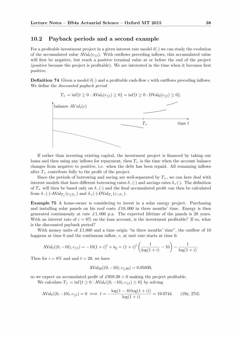
Lecture Notes – BS4a Actuarial Science – Oxford MT 2015 38
10.2 Payback periods and a second example
For a profitable investment project in a given interest rate model δ(·) we can study the evolutionof the accumulated value AValt(c≤t). With outflows preceding inflows, this accumulated valuewill first be negative, but reach a positive terminal value at or before the end of the project(positive because the project is profitable). We are interested in the time when it becomes firstpositive.
Definition 74 Given a model δ(·) and a profitable cash-flow c with outflows preceding inflows.We define the discounted payback period
T+ = inf{t ≥ 0 : AValt(c≤t) ≥ 0} = inf{t ≥ 0 : DVal0(c≤t) ≥ 0}.
-
time t
6balance AV alt(c)
T+
If rather than investing existing capital, the investment project is financed by taking outloans and then using any inflows for repayment, then T+ is the time when the account balancechanges from negative to positive, i.e. when the debt has been repaid. All remaining inflowsafter T+ contribute fully to the profit of the project.
Since the periods of borrowing and saving are well-separated by T+, we can here deal withinterest models that have different borrowing rates δ−(·) and savings rates δ+(·). The definitionof T+ will then be based only on δ−(·) and the final accumulated profit can then be calculatedfrom δ−(·)-AValT+(c≤T+) and δ+(·)-DValT+(c>T+).
Example 75 A home-owner is considering to invest in a solar energy project. Purchasingand installing solar panels on his roof costs £10, 000 in three months’ time. Energy is thengenerated continuously at rate £1, 000 p.a. The expected lifetime of the panels is 20 years.With an interest rate of i = 8% on the loan account, is the investment profitable? If so, whatis the discounted payback period?
With money units of £1,000 and a time origin “in three months’ time”, the outflow of 10happens at time 0 and the continuous inflow, c, at unit rate starts at time 0:
AValt((0,−10), c≤t) = −10(1 + i)t + st| = (1 + i)t(
1
log(1 + i)− 10
)− 1
log(1 + i).
Then for i = 8% and and t = 20, we have
AVal20((0,−10), c≤20) = 0.95939,
so we expect an accumulated profit of £959.39 > 0 making the project profitable.We calculate T+ = inf{t ≥ 0 : AValt((0,−10), c≤t) ≥ 0} by solving
AValt((0,−10), c≤t) = 0 ⇐⇒ t = − log(1− 10 log(1 + i))
log(1 + i)= 19.0744 (19y, 27d)
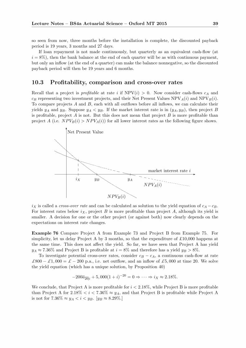
Lecture Notes – BS4a Actuarial Science – Oxford MT 2015 39
so seen from now, three months before the installation is complete, the discounted paybackperiod is 19 years, 3 months and 27 days.
If loan repayment is not made continuously, but quarterly as an equivalent cash-flow (ati = 8%), then the bank balance at the end of each quarter will be as with continuous payment,but only an inflow (at the end of a quarter) can make the balance nonnegative, so the discountedpayback period will then be 19 years and 6 months.
10.3 Profitability, comparison and cross-over rates
Recall that a project is profitable at rate i if NPV(i) > 0. Now consider cash-flows cA andcB representing two investment projects, and their Net Present Values NPVA(i) and NPVB(i).To compare projects A and B, each with all outflows before all inflows, we can calculate theiryields yA and yB. Suppose yA < yB. If the market interest rate is in (yA, yB), then project Bis profitable, project A is not. But this does not mean that project B is more profitable thanproject A (i.e. NPVB(i) > NPVA(i)) for all lower interest rates as the following figure shows.
-market interest rate i
6Net Present Value
iX yB yA
NPVB(i)
NPVA(i)
iX is called a cross-over rate and can be calculated as solution to the yield equation of cA− cB.For interest rates below iX , project B is more profitable than project A, although its yield issmaller. A decision for one or the other project (or against both) now clearly depends on theexpectations on interest rate changes.
Example 76 Compare Project A from Example 73 and Project B from Example 75. Forsimplicity, let us delay Project A by 3 months, so that the expenditure of £10,000 happens atthe same time. This does not affect the yield. So far, we have seen that Project A has yieldyA ≈ 7.36% and Project B is profitable at i = 8% and therefore has a yield yB > 8%.
To investigate potential cross-over rates, consider cB − cA, a continuous cash-flow at rate£800−£1, 000 = £− 200 p.a., i.e. net outflow, and an inflow of £5, 000 at time 20. We solvethe yield equation (which has a unique solution, by Proposition 40)
−200a20|i + 5, 000(1 + i)−20 = 0⇒ · · · ⇒ iX ≈ 2.18%.
We conclude, that Project A is more profitable for i < 2.18%, while Project B is more profitablethan Project A for 2.18% < i < 7.36% ≈ yA, and that Project B is profitable while Project Ais not for 7.36% ≈ yA < i < yB. [yB ≈ 8.29%.]

Lecture Notes – BS4a Actuarial Science – Oxford MT 2015 40
10.4 Reasons for different yields/profitability curves
For much of the interest rate modelling developments, it is instructive to think that at least themost secure savings/investment opportunities in the real world are consistent with an underlyingtime-varying force of interest. Examples in this lecture seemed to suggest otherwise. In thissection we collect a variety of remarks, some of which motivate further developments of thiscourse and should be considered again after relevant concepts have been introduced.
• There are many government bonds with a variety of redemption dates. We will indeedextract from such prices a consistent system, an implied term structure of interest rates.Even though this provides an interest rate model for a few decades, this model is subjectto uncertainty that manifests itself e.g. in that the implied rate for a fixed future year willvary from day to day, month to month, between now and in a year’s time, say. A moreappropriate model that captures this uncertainty, is a stochastic interest rate model.
• In an efficient market with participants optimizing their profit, any definitely “profitable”investment project should involve something that is as yet unaccounted for. Otherwise,many market participants would engage in it and market forces would push up prices(or affect other parts of underlying cash-flow) and remove the profit. We will investigaterelated reasoning in a lecture on arbitrage-free pricing.
• Unlike our toy examples, assessment of genuine business ventures will have to includeallowances for personal labour, administration costs etc. Such expenditure and indeedmany other positions in the cash-flows will be subject to some uncertainty. A higher yieldof a business venture may be due to a higher risk. As an example of such risk, we willinvestigate the risk of default, i.e. the risk that an income stream stops due to bankruptcyof the relevant party.
• The reason why there is a cross-over rate in Example 76 is that the cash-flow of ProjectA is more weighted towards later times, due to the big inflow after 20 years. As such, itsNPV reacts more strongly to changes in interest rates. We will investigate related notionsof Discounted Mean Term and volatility of a cash-flow, also referred to as duration.
Lecture 11
From uncertainty and corporatebonds to modelling future lifetimes
Reading: Gerber Sections 2.1, 2.2, 2.4, 3.1, 3.2, 4.1
In this lecture we introduce and apply actuarial notation for lifetime distributions.
11.1 Introduction to life insurance
The lectures that follow are motivated by the following problems.
1. An individual aged x would like to buy a life annuity (e.g. a pension) that pays him afixed amount N p.a. for the rest of his life. How can a life insurer determine a fair pricefor this product?
2. An individual aged x would like to buy a whole life insurance that pays a fixed amount Sto his dependants upon his death. How can a life insurer determine a fair single or annualpremium for this product?
3. Other related products include pure endowments that pay an amount S at time n providedan individual is still alive, an endowment assurance that pays an amount S either uponan individual’s death or at time n whichever is earlier, and a term assurance that pays anamount S upon an individual’s death only if death occurs before time n.
The material so far has been mainly deterministic in the sense that it was generally assumed thatcash-flows as well as interest rates were known, not necessarily constant, but with variabilitygiven by a time-varying rate or force of interest. In practice, such situations arise when analysingthe past or when doing a scenario analysis of the future.
This time, we need to introduce some randomness in order to model an individual’s time ofdeath, but also a company’s insolvency time.
The answer to these questions will depend on the chosen model of the future lifetime Tx ofthe individual.
41

Lecture Notes – BS4a Actuarial Science – Oxford MT 2015 42
11.2 Valuation under uncertainty
In practice, at least some part of a cash-flow is unknown in advance, or at least subject to someuncertainty. The following definition provides a suitably general framework.
Definition 77 A random vector ((Tj , Cj), 1 ≤ j ≤ N) of times Tj ∈ [0,∞) and amountsCj ∈ R possibly with random length N is called a (discrete) random cash-flow. A randomlocally Riemann integrable function C : [0,∞) → R of payment rates C(t) at time t ≥ 0 iscalled a (continuous) random cash-flow.
11.2.1 Examples
Example 78 Suppose, you are offered a zero-coupon bond of £100 nominal redeemable at parat time 1. Current market interest rates are 4%, but there is also a 10% risk of default, in whichcase no redemption payment takes place. What is the fair price?
The present value of the bond is 0 with probability 0.1 and 100(1.04)−1 with probability0.9. The weighted average A = 0.1 × 0 + 0.9 × 100(1.04)−1 ≈ 86.54 is a sensible candidate forthe fair price.
Definition 79 In an interest model δ(·), the fair premium for a random cash-flow (of fixedlength)
C = ((T1, C1), . . . , (Tn, Cn))
(typically of benefits Cj ≥ 0) is the mean value
A = E (DVal0(C)) =n∑j=1
E (Cjv(Tj))
where v(t) = exp{−∫ t0 δ(s)ds} is the discount factor at time t.
Example 80 If the times of a random cash-flow are deterministic Tj = tj and only the amountsCj are random, the fair premium is
A =n∑j=1
E(Cj)v(tj)
and depends only on the mean amounts, since the deterministic vtj can be taken out of theexpectation. Such a situation arises for share dividends.
Example 81 If the amounts of a random cash-flow are fixed Cj = cj and only the times Tjare random, the fair premium is
A =n∑j=1
cjE(v(Tj))
and in the case of constant δ we have E(v(Tj)) = E(exp{−δTj}) = E(vTj ) which is the so-calledLaplace transform or (moment) generating function. Such a situation arises for life insurancepayments, where usually a single payment is made at the time of death.
Lecture Notes – BS4a Actuarial Science – Oxford MT 2015 43
The fair premium is just an average of possible values, i.e. the actual random value ofthe cash-flow C is higher or lower with positive probability each as soon as DVal0(C) is trulyrandom. In a typical insurance framework when Cj ≥ 0 represents benefits that the insurer hasto pay us under the policy, we will be charged a premium that is higher than the fair premium,since the insurer has (expenses that we neglect and) the risk to bear that we want to get rid ofby buying the policy.
Call A+ the higher premium that is to be determined. Clearly, the insurer is concerned abouthis loss (DVal0(C)−A+)+, or expected loss E (DVal0(C)−A+)+. In some special cases this canbe evaluated, sometimes the quantity under the expectation is squared (so-called squared loss).A simpler quantity is the probability of loss P(DVal0(C) > A+). One can use Tchebychev’sinequality to demonstrate that the insurer’s risk of loss gets smaller with the larger the numberof policies.
11.2.2 Uncertain payment
The following is an important special case of Example 80 which motivates lifetime modellingand corporate bond pricing.
As you will see the pricing of corporate bonds is not too different to the pricing of lifeinsurance products. In both cases there is a random time when the cash-flows cease, time ofinsolvency and time of death respectively.
Example 82 Let tj be fixed and
Cj =
{cj with probability pj ,0 with probability 1− pj .
So we can say Cj = Bjcj , where Bj is a Bernoulli random variable with parameter pj , i.e.
Bj =
{1 with probability pj ,0 with probability 1− pj .
For the random cash-flow C = ((t1, B1c1), . . . , (tn, Bncn)), we have
A =
n∑j=1
E(Bjcjv(tj)) =
n∑j=1
cjv(tj)E(Bj) =
n∑j=1
pjcjv(tj).
Note that we have not required the Bj to be independent (or assumed anything about theirdependence structure).
11.3 Pricing of corporate bonds
Letc = ((1, DN), . . . , (n− 1, DN), (n,DN +N))
be a simple fixed-interest security(eg a bond) issued by a company. If the company goesinsolvent, all future payments are lost. So we may wish to look at the random cash-flow
((1, DNB1), . . . , (n− 1, DNBn−1), (n, (DN +N)Bn)),
Lecture Notes – BS4a Actuarial Science – Oxford MT 2015 44
where Bj = I(T > j) and T is a random variable representing the insolvency time;
pj = P(Bj = 1) = P(T > j) = F T (j).
Here and in the sequel, we will use the following notation for continuous probability distribu-tions: let T be a continuous random variable taking values in [0,∞), modelling a lifetime orinsolvency time. Its distribution function and survival function are given by
FT (t) = P(T ≤ t) and F T (t) = P(T > t) = 1− FT (t),
while its density function satisfies
fT (t) =d
dtFT (t) = − d
dtF T (t), FT (t) =
∫ t
0fT (s)ds, F T (t) =
∫ ∞t
fT (s)ds.
Definition 83 The function
µT (t) =fT (t)
F T (t), t ≥ 0,
specifies the force of mortality or hazard rate at (time) t.
Proposition 84 We have1
εP(T ≤ t+ ε|T > t)→ µT (t) as ε→ 0.
Proof: We use the definitions of conditional probabilities and differentiation:
1
εP(T ≤ t+ ε|T > t) =
1
ε
P(T > t, T ≤ t+ ε)
P(T > t)=
1
ε
P(T ≤ t+ ε)− P(T ≤ t)P(T > t)
=1
F T (t)
FT (t+ ε)− FT (t)
ε−→
F ′T (t)
F T (t)=
fT (t)
F T (t)= µT (t).
2
So, we can say informally that P(T ∈ (t, t+ dt)|T > t) ≈ µT (t)dt, i.e. µT (t) represents for eacht ≥ 0 the current “rate of dying” (or bankruptcy etc.) given survival up to t.
Example 85 The exponential distribution of rate µ is given by
FT (t) = 1− e−µt, F T (t) = e−µt, fT (t) = µe−µt, µT (t) =µe−µt
e−µt= µ constant.
Lemma 86 We have F T (t) = exp
(−∫ t
0µT (s)ds
).
Proof: First note that F T (0) = P(T > 0) = 1. Also
d
dtlogF T (t) =
F′T (t)
F T (t)=−fT (t)
F T (t)= −µT (t).
So
logF T (t) = logF T (0) +
∫ t
0
d
dslogF T (s)ds = 0 +
∫ t
0−µT (s)ds.
2
Lecture Notes – BS4a Actuarial Science – Oxford MT 2015 45
Let c be a deterministic cash-flow on [0,∞) and consider c[0,T ), the cash-flow “killed” at timeT : all events from time T on are cancelled. If T is random, c[0,T ) is a random cash-flow.
Proposition 87 Let δ(·) be an interest rate model, c a cash-flow and T a continuous insolvencytime, then
E(δ-Val0
(c[0,T )
))= δ-Val0(c)
where δ(t) = δ(t) + µT (t) and µ(t) = fT (t)/F T (t).
Proof: Let c = ((tj , cj), j ≥ 1). Then
δ-Val0(c) =∑j≥1
cjv(tj), where v(tj) = exp
(−∫ tj
0δ(s)ds
),
andδ-Val0(c[0,T )) =
∑j≥1
cjv(tj)I(T > tj),
so that
E(δ-Val0(c[0,T ))
)=∑j≥1
cjv(tj)E(I(T > tj)), where E(I(T > tj)) = P(T > tj) = F T (tj).
By the previous lemma, the main expression equals∑j≥1
cj exp
(−∫ tj
0δ(s)ds
)exp
(−∫ tj
0µT (s)ds
)=∑j≥1
cj exp
(−∫ tj
0δ(s)ds
)= δ-Val0(c).
2
The important special case is when δ and µ are constant and c is a corporate bond whosepayment stream stops at the insolvency time T .
Corollary 88 Given a constant δ model, the fair price for a corporate bond C with insolvencytime T ∼ Exp(µ) is
A = E(δ-DVal0(C)) = δ-DVal0(c)
where δ = δ + µ.
Often, problems arise in a discretised way. Remember that a geometric random variablewith parameter p can be thought of as the first 0 in a series of Bernoulli 0-1 trials with success(1) probability p.
Proposition 89 Let c be a discrete cash-flow with tk ∈ N for all k = 1, . . . , n, T ∼ geom(p),i.e. P(T = k) = pk−1(1− p), k = 1, 2, . . .. Then in the constant i model,
E(i-Val0(c[0,T ))
)= j-Val0(c)
where j = (1 + i− p)/p.
Proof: P(T > k) = pk. Therefore
E(i-Val0(c[0,T ))
)=
n∑k=1
ptkck(1 + i)−tk .
2

Lecture Notes – BS4a Actuarial Science – Oxford MT 2015 46
11.4 Expected yield
For deterministic cash-flows that can be interpreted as investment deals (or loan schemes), wedefined the yield as an intrinsic rate of return. For a random cash-flow, this notion gives arandom yield which is usually difficult to use in practice. Instead, we define:
Definition 90 Let C be a random cash-flow. The expected yield of C is the interest ratei ∈ (−1,∞), if it exists and is unique such that
E(NPV(i)) = 0,
where NPV(i) = i-Val0(C) denotes the net present value of C at time 0 discounted at interestrate i.
This corresponds to the yield of the “average cash-flow”. Note that this terminology may bemisleading – this is not the expectation of the yield of C, even if that were to exist.
Example 91 An investment of £500, 000 provides
• a continuous income stream of £50, 000 per year, starting at an unknown time S andending in 6 years’ time;
• a payment of unknown size A in 6 years’ time.
Suppose that
• S is uniformly distributed between [2years, 3years] (time from now);
• the mean of A is £700, 000.
What is the expected yield?We use units of £10, 000 and 1 year. The time-0 value at rate y is
−50 +
∫ 6
s=S5(1 + y)−sds+ (1 + y)−6A.
The expected time-0 value is
−50 +
∫ 6
s=2P(S < s)5(1 + y)−sds+ (1 + y)−6E(A)
= −50 +
∫ 3
s=2(s− 2)5(1 + y)−sds+
∫ 6
s=35(1 + y)−sds+ (1 + y)−670 =: f(y).
Set f(y) = 0 and find
f(10.45%) = 0.1016... and f(10.55%) = −0.1502...
So the expected yield is 10.5% to 1d.p. (note that we only need to use the mean of A).
As a consequence of Proposition 89, we note:
Corollary 92 If T ∼ geom(p) and c a cash-flow at integer times with yield y(c), then theexpected yield of c[0,T ) is p(1 + y(c))− 1.
Proof: Note that y(c)-Val0(c) = 0, and by Proposition 89, we have E(i-Val0(c[0,T )) = 0, ify(c) = (1 + i− p)/p, i.e. 1 + i = p(1 + y(c)), as required. Also, this is the unique solution to theexpected yield equation as otherwise the relationship 1 + i = p(1 + j) would give more solutionsto the yield equation. 2

Lecture Notes – BS4a Actuarial Science – Oxford MT 2015 47
11.5 Lives aged x
Now we are back to life-insurance products.Recall our standard notation for continuous lifetime distributions. For a continuously dis-
tributed random lifetime T , we write FT (t) = P(T ≤ t) for the cumulative distribution function,fT (t) = F ′T (t) for the probability density function, F T (t) = P(T > t) for the survival functionand µT (t) = fT (t)/F T (t) for the force of mortality. Let us write ωT = inf{t ≥ 0 : F T (t) = 0}for the maximal possible lifetime. Also recall
F T (t) = exp
(−∫ t
0µT (s)ds
).
We omit index T if there is no ambiguity.Suppose now that T models the future lifetime of a new-born person. In life insurance
applications, we are often interested in the future lifetime of a person aged x, or more preciselythe residual lifetime T − x given {T > x}, i.e. given survival to age x. For life annuities thisdetermines the random number of annuity payments that are payable. For a life assurancecontract, this models the time of payment of the sum assured. In practice, insurance companiesperform medical tests and/or collect employment/geographical/medical data that allow moreaccurate modelling. However, let us here assume that no such other information is available.Then we have, for each x ∈ [0, ω),
P(T − x > y|T > x) =P(T > x+ y)
P(T > x)=F (x+ y)
F (x), y ≥ 0,
by the definition of conditional probabilities P(A|B) = P(A ∩B)/P(B).It is natural to directly model the residual lifetime Tx of an individual (a life) aged x as
F x(y) = P(Tx > y) =F (x+ y)
F (x)= exp
(−∫ x+y
xµ(s)ds
)= exp
(−∫ y
0µ(x+ t)dt
).
We can read off µx(t) = µTx(t) = µ(x + t), i.e. the force of mortality is still the same, justshifted by x to reflect the fact that the individual aged x and dying at time Tx is aged x+ Txat death. We can also express cumulative distribution functions
Fx(y) = 1− F x(y) =F (x)− F (x+ y)
F (x)=F (x+ y)− F (x)
1− F (x),
and probability density functions
fx(y) =
{F ′x(y) = f(x+y)
1−F (x) = f(x+y)
F (x), 0 ≤ y ≤ ω − x,
0, otherwise.
There is also actuarial lifetime notation, as follows
tqx = Fx(t), tpx = 1− tqx = F x(t), qx = 1qx, px = 1px, µx = µ(x) = µx(0).
In this notation, we have the following consistency condition on lifetime distributions for differ-ent ages:
Proposition 93 For all x ≥ 0, s ≥ 0 and t ≥ 0, we have
s+tpx = spx × tpx+s.
Lecture Notes – BS4a Actuarial Science – Oxford MT 2015 48
By general reasoning, the probability that a life aged x survives for s + t years is the same asthe probability that it first survives for s years and then, aged x + s, survives for another tyears.
Proof: Formally, we calculate the right-hand side
spx × tpx+s = P(Tx > s)P(Tx+s > t) =P(T > x+ s)
P(T > x)
P(T > x+ s+ t)
P(T > x+ s)= P(Tx > s+ t)
= s+tpx.
2
We can also express other formulas, that we have already established, in actuarial notation:
fx(t) = tpxµx+t, tpx = exp
(−∫ t
0µx+sds
), tqx =
∫ t
0spxµx+sds.
The first one says that to die at t, life x must survive for time t and then die instantaneously.
11.6 Curtate lifetimes
In practice, many cash flows pay at discrete times, often at the end of each month. Let usbegin here by discretising continuous lifetimes to integer-valued lifetimes. This is often done inpractice, with interpolation being used for finer models.
Definition 94 Given a continuous lifetime random variable Tx, the random variable Kx = [Tx],where [·] denotes the integer part, is called the associated curtate lifetime.
Of course, one can also model curtate lifetimes directly. Note that, for continuously dis-tributed Tx
P(Kx = k) = P(k ≤ Tx < k + 1) = P(k < Tx ≤ k + 1) = kpx × qx+k.
Also, by Proposition 93,
P(Kx ≥ k) = kpx =
k−1∏j=0
px+j ,
i.e. Kx can be thought of as the number of successes before the first failure in a sequence ofindependent Bernoulli trials with varying success probabilities px+j , j ≥ 0. Here, success is thesurvival of a year, while failure is death during the year.
Proposition 95 We have E(Kx) =
[ω−x]∑k=1
kpx.
Proof: By definition of the expectation of a discrete random variable,
[ω−x]∑k=1
kpx =
[ω−x]∑k=1
P(Kx ≥ k) =
[ω−x]∑k=1
[ω−x]∑m=k
P(Kx = m)
=
[ω−x]∑m=1
m∑k=1
P(Kx = m) =
[ω−x]∑m=0
mP(Kx = m) = E(Kx).
2

Lecture Notes – BS4a Actuarial Science – Oxford MT 2015 49
Example 96 If T is exponentially distributed with parameter µ ∈ (0,∞), then K = [T ] isgeometrically distributed:
P(K = k) = P(k ≤ T < k + 1) = e−kµ − e−(k+1)µ = (e−µ)k(1− e−µ), k ≥ 0.
We identify the parameter of the geometric distribution as e−µ. Note also that here px = e−µ
and qx = 1− e−µ for all x.
In general, we get
P(Kx ≥ k) =
k−1∏j=0
px+j = kpx = exp
(−∫ k
0µ(x+ t)dt
)=
k−1∏j=0
exp
(−∫ x+j+1
x+jµ(s)ds
),
so that we read off
px = exp
(−∫ x+1
xµ(s)ds
), x ≥ 0.
In practice, µ is often assumed constant between integer points (denoted µx+0.5) or continuouspiecewise linear between integer points.
11.7 Examples
Let us now return to our motivating problem.
Example 97 (Whole life insurance) Let Kx be a curtate future lifetime. A whole life in-surance pays one unit at the end of the year of death, i.e. at time Kx + 1. In the model of aconstant force of interest δ, the random discounted value at time 0 is Z = e−δ(Kx+1), so the fairpremium for this random cash-flow is
Ax = E(Z) = E(e−δ(Kx+1)) =∞∑k=1
e−δkP(Kx = k − 1) =∞∑m=0
(1 + i)−m−1mpxqx+m,
where i = eδ − 1 and Ax is just the actuarial notation for this expected discounted value.
Lecture 12
Lifetime distributions and life-tables
Reading: Gerber Sections 2.3, 2.5, 3.2
In this lecture we give an introduction to life-tables. We will not go into the details of con-structing life-tables, which is one of the subjects of BS3b Statistical Lifetime-Models. What weare mostly interested in is the use of life-tables to price life insurance products.
12.1 Actuarial notation for life products.
Recall the motivating problems. Let us introduce the associated notation.
Example 98 (Term assurance, pure endowment and endowment) The fair premium ofa term insurance is denoted by
A1x:n| =
n−1∑k=0
vk+1kpxqx+k.
The superscript 1 above the x indicates that 1 is only paid in case of death within the periodof n years.
The fair premium of a pure endowment is denoted by A 1x:n| = vnnpx. Here the superscript 1
indicates that 1 is only paid in case of survival of the period of n years.The fair premium of an endowment is denoted by Ax:n| = A1
x:n|+A 1x:n|, where we could have
put a 1 above both x and n, but this is omitted being the default, like in previous symbols.
Example 99 (Life annuities) Given a constant i interest model, the fair premium of anordinary (respectively temporary) life annuity for a life aged x is given by
ax =
∞∑k=1
vkkpx respectively ax:n| =
n∑k=1
vkkpx.
For an ordinary (respectively temporary) life annuity-due, an additional certain payment attime 0 is made (and any payment at time n omitted):
ax = 1 + ax respectively ax:n| = 1 + ax:n−1|.
50
Lecture Notes – BS4a Actuarial Science – Oxford MT 2015 51
12.2 Simple laws of mortality
As we have seen, the theory is nicest for exponentially distributed lifetimes. However, theexponential distribution is not actually a good distribution to model human lifetimes:
• One reason that we have seen is that the curtate lifetime is geometric, i.e. each year givensurvival up to then, there is the same probability of dying in the next year. In practice,you would expect that this probability increases for higher ages.
• There is clearly significantly positive probability to survive up to age 70 and zero proba-bility to survive to age 140, and yet the exponential distribution suggests that
P(T > 140) = e−140µ = (e−70µ)2 = (P(T > 70))2.
Specifically, if we think there is at least 50% chance of a newborn to survive to age 70,there would be at least 25% chance to survive to age 140; if we think that the averagelifetime is more than 70, then µ < 1/70, so P(T > 140) > e−2 > 10%.
• More formally, the exponential distribution has the lack of memory property, which heresays that the distribution of Tx is still exponential with the same parameter, independentof x. This would mean that there is no ageing.
These observations give some ideas for more realistic models. Generally, we would favour modelswith an eventually increasing force of mortality (in reliability theory such distributions are calledIFR distributions – increasing failure rate).
1. Gompertz’ Law: µ(t) = Bct for some B > 0 and c > 1.
2. Makeham’s Law: µ(t) = A + Bct for some A ≥ 0, B > 0 and c > 1 (or c > 0 to includeDFR – decreasing failure rate cases).
3. Weibull: µ(t) = ktβ for some k > 0 and β > 0.
Makeham’s Law actually gives a reasonable fit for ages 30-70.
12.3 The life-table
Suppose we have a population of newborn individuals (or individuals aged α > 0, some lowestage in the table). Denote the size of the population by `α. Then let us observe each year thenumber `x of individuals still alive, until the age when the last individual dies reaching `ω = 0.Then out of `x individuals, `x+1 survived age x, and the proportion `x+1/`x can be seen as theprobability for each individual to survive. So, if we set
px = `x+1/`x for all α ≤ x ≤ ω − 1.
we specify a curtate lifetime distribution. The function x 7→ `x is usually called the life-tablein the strict sense. Note that also vice versa, we can specify a life-table with any given curtatelifetime distribution by choosing `0 = 100, 000, say, and setting `x = `0 × xp0. In this case, weshould think of `x as the expected number of individuals alive at age x. Strictly speaking, weshould distinguish px and its estimate px = `x+1/`x, but this notion had not been developedwhen actuaries first did this, and rather leave the link to statistics and the interpretation of `x
Lecture Notes – BS4a Actuarial Science – Oxford MT 2015 52
as an observed quantity, which it usually isn’t anyway for real life-tables that were set up byrather more sophisticated methods.
There is a lot of notation associated with life-tables, and the 1967/70 life-table that wewill work with actually consists of several pages of tables of different life functions. We workwith the table for qx, and there is also a table containing all `x, or indeed dx = `x − `x+1,α ≤ x ≤ ω − 1. Observe that, with this notation, qx = dx/`x.
See Figure 12.1 for plots of hazard function (x 7→ qx) and probability mass functions (x 7→P(K = x)). Note that initially and up to age 35, the one-year death probabilities are below0.001, then increase to cross 0.1 at age 80 and 0.5 at age 100.
12.4 Example
We will look at the 1967/70 life-table in more detail in the next lecture. Let us finish thislecture by giving an (artificial) example of a life-table constructed from a parametric family. Amore realistic example is on the next assignment sheet.
Example 100 We find records about a group of 10,000 from when they were all aged 20, whichreveal that 8,948 were still alive 5 years later and 7,813 another 5 years later. This means, thatwe are given
`20 = 10, 000, `25 = 8, 948 and `30 = 7, 813.
Of course, this is not enough to set up a life-table, since all we would be able to calculate is
5p20 =`25`20
= 0.895 and 5p25 =`30`25
= 0.873.
However, if we assume that the population has survival function
F T (t) = exp(−Ax−Bx2), for some A ≥ 0 and B ≥ 0,
we can solve two equations to identify the parameters that exactly replicate these two proba-bilities:
5p20 = P(T > 25|T > 20) =exp(−25A− 252B)
exp(−20A− 202B)= exp(−5A− 225B)
pp25 = exp(−5A− 275B).
(More sophisticated statistical techniques are beyond the scope of this course.) Here, we obtainthat
B =ln(0.895)− ln(0.873)
50= 0.00049 and A =
− ln(0.895)− 225B
5= 0.00018,
and we can then construct the whole associated lifetable as
`x = `20 × x−20p20 = 10, 000 exp(−(x− 20)A− (x2 − 202)B).
The reliability away from x ∈ [20, 30] must be questioned, but we can compute the implied`100 = 89.29.
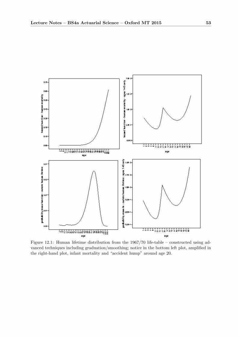
Lecture Notes – BS4a Actuarial Science – Oxford MT 2015 53
Figure 12.1: Human lifetime distribution from the 1967/70 life-table – constructed using ad-vanced techniques including graduation/smoothing; notice in the bottom left plot, amplified inthe right-hand plot, infant mortality and “accident hump” around age 20.
Lecture 13
Select life-tables and applications
Reading: Gerber 2.5, 2.6
13.1 Select life-tables
Some life-tables are select tables, meaning that mortality rates depend on the duration fromjoining the population. This is relevant if there is e.g. a medical check at the policy start date,which can reject applicants with poor health and only offer policies to applicants with betterthan average health and lower than average mortality, at least for the next few years. We denoteby
• [x] the age at the date of joining the population;
• q[x] the mortality rate for a life aged x having joined the population at age x;
• q[x]+j the mortality rate for a life aged x+ j having joined the population at age x;
• qx+r the ultimate mortality for a life aged x having joined the population at age x;
It is supposed that after some select period of r years, mortality no longer varies significantlywith duration since joining, but only with age: this is the ultimate portion of the table.
Example 101 The 1967/70 life-table has three columns, two select columns for q[x] and q[x]+1
and one ultimate column for qx+2. To calculate probabilities for K[x], the relevant entries arethe three entries in row [x] and all ultimate entries below this row. E.g.
P(K[x] = 4) = (1− q[x])(1− q[x]+1(1− qx+2)(1− qx+3)qx+4.
Using the excerpt of Figure 13.1 of the table for an age [55], we obtain specifically
P(K[55] = 4) = (1− 0.00447)(1− 0.00625)(1− 0.01050)(1− 0.01169)0.01299 ≈ 0.01257.
Example 102 Consider a 4-year temporary life assurance issued to a checked life [55]. Assum-ing a constant interest rate of i = 4%, we calculate
A 1[55]:4|
= vq[55] + v2p[55]q[55]+1 + v3p[55]p[55]+1q57 + v4p[55]p[55]+1p57q58 = 0.029067.
Therefore, the fair price of an assurance with sum assured N = £100, 000 is £2, 906.66, payableas a single up-front premium.
54

Lecture Notes – BS4a Actuarial Science – Oxford MT 2015 55
Age [x]
5354555657
5859606162
q[x]
.00376288
.00410654
.00447362
.00486517
.00528231
.00572620
.00619802
.00669904
.00723057
.00779397
q[x]+1
.00519413
.00570271
.00625190
.00684424
.00748245
.00816938
.00890805
.00970168
.01055365
.01146756
qx+2
.00844128
.00941902
.01049742
.01168566
.01299373
.01443246
.01601356
.01774972
.01965464
.02174310
Age x+ 2
5556575859
6061626364
Figure 13.1: Extract from mortality tables of assured lives based on 1967-70 data.
13.2 Multiple premiums
We will return to a more complete discussion of multiple premiums later, but for the purposeof this section, let us define:
Definition 103 Given a constant i interest model, let C be the cash flow of insurance benefits,the annual fair level premium of C is defined to be
Px =E(DV al0(C))
ax.
This definition is based on the following principles:
Proposition 104 In the setting of Definition 103, the expected dicounted benefits equal theexpected discounted premium payments. Premium payments stop upon death.
Proof: The expected discounted value of premium payments ((0, Px), . . . , (Kx, Px)) is Pxax =E(DV al0(C)). 2
Example 105 We calculate the fair annual premium in Example 102. Since there should notbe any premium payments beyond when the policy ends either by death or by reaching the endof term, the premium payments form a effectively a temporary life annuity-due, i.e. cash flow((0, 1), (1, 1), (2, 1), (3, 1)) restricted to the lifetime K[55]. First
a[55]:4| = 1 + vp[55] + v2p[55]p[55]+1 + v3p[55]p[55]+1p57 ≈ 3.742157
and the annual premium is therefore calculated from the life table in Figure 13.1 as
P =NA 1
[55]:4|
a[55]:4|= 776.73.

Lecture Notes – BS4a Actuarial Science – Oxford MT 2015 56
13.3 Interpolation for non-integer ages x+ u, x ∈ N, u ∈ (0, 1)
There are two popular models. Model 1 is to assume that the force of mortality µt is constantbetween each (x, x+ 1), x ∈ N. This implies
px = exp
(−∫ x+1
xµtdt
)= exp (−µx+0.5) ⇒ µx+ 1
2= − ln(px).
Also, for 0 ≤ u ≤ 1,
P(T > x+ u|T > x) = exp
{−∫ x+u
xµtdt
}= exp {−uµx+0.5} = (1− qx)u,
and with notation T = K+S, where K = [T ] is the integer part and S = {T} = T−[T ] = T−Kthe fractional part of T , this means that
P(S ≤ u|K = x) =P(x ≤ T ≤ x+ u)/P(T > x)
P(x ≤ T < x+ 1)/P(T > x)=
1− exp {−uµx+0.5}1− exp {−µx+0.5}
, 0 ≤ u ≤ 1,
a distribution that is in fact the exponential distribution with parameter µx+0.5, truncated atω = 1: for exponentially distributed E
P(E ≤ u|E ≤ 1) =P(E ≤ u)
P(E ≤ 1)=
1− exp {−uµx+0.5}1− exp {−µx+0.5}
, 0 ≤ u ≤ 1.
Since the parameter depends on x, S is not independent of K here.Model 2 is convenient e.g. when calculating variances of continuous lifetimes: we assume
that S and K are independent, and that S has a uniform distribution on [0, 1]. Mathematicallyspeaking, these models are not compatible: in Model 2, we have, instead, for 0 ≤ u ≤ 1,
FTx(u) = P(T > x+ u|T > x)
= P(K ≥ x+ 1|K ≥ x) + P(S > u|K = x)P(K = x|T > x)
= (1− qx) + (1− u)qx = 1− uqx.
We then calculate the force of mortality at x+ u as
µx+u = −F ′Tx(u)
FTx(u)=
qx1− uqx
and this is increasing in u. Note that µ is discontinuous at (some if not all) integer times. Theonly exception is very artificial, as we require qx+1 = qx/(1 − qx), and in order for this to notexceed 1 at some point, we need q0 = α = 1/n, and then qk = α
1−kα , k = 1, . . . , n − 1, withω = n maximal age. Usually, one accepts discontinuities.
If one of the two assumptions is satisfied, the above formulas allow to reconstruct the fulldistribution of a lifetime T from the entries (qx)x∈N of a life-table: from the definition ofconditional probabilities
P(S ≤ t− [t]|K = [t]) =P(K = [t], S ≤ t− [t])
P(K = [t])=
1− e−(t−[t])µx+0.5
1− e−µx+0.5in Model 1,
t− [t] in Model 2,
we deduce that
P(T ≤ t) = P(K ≤ [t]− 1) + P(K = [t])P(S ≤ t− [t]|K = [t]),
and we have already expressed the distribution of K in terms of (qx)x∈N.

Lecture Notes – BS4a Actuarial Science – Oxford MT 2015 57
13.4 Practical concerns
• Mortality depends on individual characteristics (rich, athletic, adventurous). Effects onmortality can be studied. Models include scaling or shifting already existing tables as afunction of the characteristics
• We need to estimate future mortality, which may not be the same as current or pastmortality. Note that this is inherently two-dimensional: a 60-year old in 2060 is likely tohave a different mortality from a 60-year old in 2010. A two-dimensional life-table shouldbe indexed separately by calender year of birth and age, or current calender year and age.Prediction of future mortality is a major actuarial problem. Extrapolating substantiallyinto the future is subject to considerable uncertainty.
• There are other risks, such as possible effects of pills to halt ageing, or major influenzaoutbreak. How can such risks be hedged?
Lecture 14
Evaluation of life insurance products
Reading: Gerber Sections 3.2, 3.3, 3.4, 3.5, 3.6, 4.2
14.1 Life assurances
Recall that the fair single premium for a whole life assurance is
Ax = E(vKx+1) =∞∑k=0
vk+1kpxqx+k,
where v = e−δ = (1 + i)−1 is the discount factor in the constant-i model. Note also that highermoments of the present value are easily calculated. Specifically, the second moment
2Ax = E(v2(Kx+1)),
associated with discount factor v2, is the same as Ax calculated at a rate of interest i′ =(1 + i)2 − 1, and hence
Var(vKx+1) = E(v2(Kx+1))−(E(vKx+1)
)2= 2Ax − (Ax)2.
Remember that the variance as expected squared deviation from the mean is a quadratic quan-tity and mean and variance of a whole life assurance of sum assured S are
E(SvKx+1) = SAx and Var(SvKx+1) = S2Var(vKx+1) = S2( 2Ax − (Ax)2).
Similarly for a term assurance,
E(SvKx+11{Kx<n}
)= SA1
x:n| and Var(SvKx+11{Kx<n}
)= S2
(2A1
x:n| − (A1x:n|)
2)
for a pure endowment
E(Svn1{Kx≥n}
)= SA 1
x:n| = Svnnpx and Var(Svn1{Kx≥n}) = S2(2A 1
x:n| − (A 1x:n|)
2)
and for an endowment assurance
E(Svmin(Kx+1,n)) = SAx:n| and Var(Svmin(Kx+1,n)) = S2(2Ax:n| − (Ax:n|)
2)
58
Lecture Notes – BS4a Actuarial Science – Oxford MT 2015 59
Note that
S2(2Ax:n| − (Ax:n|)
2)6= S2
(2A1
x:n| − (A1x:n|)
2)
+ S2(2A 1
x:n| − (A 1x:n|)
2),
because term assurance and pure endowment are not independent, quite the contrary, theproduct of their discounted values always vanishes, so that their covariance −S2A1
x:n|A1
x:n| ismaximally negative. In other notation, from the variance formula for sums of dependent randomvariables,
Var(Svmin(Kx+1,n)) = Var(SvKx+11{Kx<n} + Svn1{Kx≥n})
= Var(SvKx+11{Kx<n}) + Var(Svn1{Kx≥n}) + 2Cov(SvKx+11{Kx<n}, Svn1{Kx≥n})
= Var(SvKx+11{Kx<n}) + Var(Svn1{Kx≥n})− 2E(SvKx+11{Kx<n})E(Svn1{Kx≥n})
= S2(2A1
x:n| − (A1x:n|)
2)
+ S2(2A 1
x:n| − (A 1x:n|)
2)− S2A1
x:n|A1
x:n|.
14.2 Life annuities and premium conversion relations
Recall present values of whole-life annuities, temporary annuities and their due versions
ax =∞∑k=1
vkkpx, ax:n| =n∑k=1
vkkpx, ax = 1 + ax and ax:n| = 1 + ax:n−1|.
Also note the simple relationships (that are easily proved algebraically)
ax = vpxax+1 and ax:n| = vpxax+1:n|.
By general reasoning, they can be justified by saying that the expected discounted value ofregular payments in arrears for up to n years contingent on a life x is the same as the expecteddiscounted value of up to n payments in advance contingent on a life x + 1, discounted by afurther year, and given survival of x for one year (which happens with probability px).
To calculate variances of discounted life annuity values, we use premium conversion relations:
Proposition 106 Ax = 1− dax and Ax:n| = 1− dax:n|, where d = 1− v.
Proof: The quickest proof is based on the formula an| = (1− vn)/d from last term
ax = E(aKx+1| = E(
1− vKx+1
d
)=
1− E(vKx+1)
d=
1−Axd
.
The other formula is similar, with Kx + 1 replaced by min(Kx + 1, n). 2
Now for a whole life annuity,
Var(aKx|) = Var
(1− vKx
i
)= Var
(vKx+1
d
)=
1
d2Var(vKx+1) =
1
d2(2Ax − (Ax)2
).
For a whole life annuity-due,
Var(aKx+1|) = Var(1 + aKx|) =1
d2(2Ax − (Ax)2
).
Lecture Notes – BS4a Actuarial Science – Oxford MT 2015 60
Similarly,
Var(amin(Kx,n)|) = Var
(1− vmin(Kx,n)
i
)= Var
(vmin(Kx+1,n+1)
d
)=
1
d2
(2Ax:n+1| − (Ax:n+1|)
2)
and
Var(amin(Kx+1,n)|) = Var
(1 + a
min(Kx,n−1)|
)=
1
d2(2Ax:n| − (Ax:n|)
2).
14.3 Continuous life assurance and annuity functions
A whole of life assurance with payment exactly at date of death has expected present value
Ax = E(vTx) =
∫ ∞0
vtfx(t)dt =
∫ ∞0
vttpxµx+tdt.
An annuity payable continuously until the time of death has expected present value
ax = E(
1− vTxδ
)=
∫ ∞0
vttpxdt.
Note also the premium conversion relation Ax = 1− δax.For a term assurance with payment exactly at the time of death, we obtain
A1x:n| = E(vTx1{Tx≤n}) =
∫ n
0vttpxµx+tdt.
Similarly, variances can be expressed, as before, e.g.
Var(vTx1{Tx≤n}) = 2A1x:n| − (A
1x:n|)
2.
14.4 More general types of life insurance
In principle, we can find appropriate premiums for any cash-flow of benefits that depend on Tx,by just taking expected discounted values. An example of this was on Assignment 4, where anincreasing whole life assurance was considered that pays Kx + 1 at time Kx + 1. The purposeof the exercise was to establish the premium conversion relation
(IA)x = ax − d(Ia)x
that relates the premium (IA)x to the increasing life annuity-due that pays k + 1 at time kfor 0 ≤ k ≤ Kx. It is natural to combine such an assurance with a regular savings plan andpay annual premiums. The principle that the total expected discounted premium paymentscoincide with the total expected discounted benefits yield a level annual premium (IP )x thatsatisfies
(IP )xax = (IA)x = ax − d(Ia)x ⇒ (IP )x = 1− d(Ia)xax
.

Lecture Notes – BS4a Actuarial Science – Oxford MT 2015 61
Similarly, there are decreasing life assurances. A regular decreasing life assurance is useful tosecure mortgage payments. The (simplest) standard case is where a payment of n−Kx is dueat time Kx + 1 provided Kx < n. This is a term assurance. We denote its single premium by
(DA)1x:n| =
n−1∑k=0
(n− k)vk+1kpxqx+k
and note that
(DA)1x:n| = A1x:n| +A1
x:n−1| + · · ·+A1x:1| = nA1
x:n| − (IA)1x:n|,
where (IA)1x:n| denotes the present value of an increasing term-assurance.
Lecture 15
Premiums
Reading: Gerber Sections 5.1, 5.3, 6.2, 6.5, 10.1, 10.2
In this lecture we incorporate expenses into premium calculations. On average, such expensesare to cover the insurer’s administration cost, contain some risk loading and a profit margin forthe insurer. We assume here that expenses are incurred for each policy separately. In practice,actual expenses per policy also vary with the total number of policies underwritten. There arealso strategic variations due to market forces.
15.1 Different types of premiums
Consider the future benefits payable under an insurance contract, modelled by a random cashflow C. Recall that typically payment for the benefits are either made by a single lump sumpremium payment at the time the contract is effected (a single-premium contract) or by aregular annual (or monthly) premium payments of a level amount for a specified term (a regularpremium contract). Note that we will be assuming that all premiums are paid in advance, sothe first payment is always due at the time the policy is effected.
Definition 107 • The net premium (or pure premium) is the premium amount requiredto meet the expected benefits under a contract, given mortality and interest assumptions.
• The office premium (or gross premium) is the premium required to meet all the costsunder an insurance contract, usually including expected benefit cost, expenses and profitmargin. This is the premium which the policy holder pays.
In this terminology, the net premium for a single premium contract is the expected cost ofbenefits E(Val0(C)). E.g., the net premium for a single premium whole life assurance policy ofsum assured 1 issued to a life aged x is Ax.
In general, recall the principle that the expected present value of net premium paymentequals the expected present value of benefit payments. For office premiums, and later premiumreserves, it is more natural to write this from the insurer’s perspective as
expected present value of net premium income = expected present value of benefit outgo.
62
Lecture Notes – BS4a Actuarial Science – Oxford MT 2015 63
Then, we can say similarly
expected present value of office premium income
= expected present value of benefit outgo
+ expected present value of outgo on expenses
+ expected present value of required profit loading.
Definition 108 A (policy) basis is a set of assumptions regarding future mortality, investmentreturns, expenses etc.
The basis used for calculating premiums will usually be more cautious than the best estimatefor a number of reasons, including to allow for a contingency margin (the insurer does not wantto go bust) and to allow for uncertainty in the estimates themselves.
15.2 Net premiums
We will use the following notation for the regular net premium payable annually throughoutthe duration of the contract:
Px:n| for an endowment assurance
P 1x:n| for a term assurance
Px for a whole life assurance.
In each case, the understanding is that we apply a second principle which stipulates that thepremium payments end upon death, making the premium payment cash-flow a random cash-flow. We also introduce
nPx as regular net premium payable for a maximum of n years.
To calculate net premiums, recall that premium payments form a life annuity (temporary orwhole-life), so we obtain net annual premiums from the first principle of equal expected dis-counted values for premiums and benefits, e.g.
ax:n|Px:n| = Ax:n| ⇒ Px:n| =Ax:n|ax:n|
.
Similarly, P 1x:n| =
A1x:n|
ax:n|, Px =
Axax
, nPx =Axax:n|
.
15.3 Office premiums
For office premiums, the basis for their calculation is crucial. We are already used to makingassumptions about an interest rate model and about mortality. Expenses can be set in a varietyof ways, and often it is a combination of several expenses that are charged differently. It is oflittle value to categorize expenses by producing a list of possibilities, because whatever theirform, they describe nothing else than a cash flow, sometimes involving the premium to bedetermined. Finding the premium is solving an equation of value, which is usually a linearequation in the unknown. We give an example.
Lecture Notes – BS4a Actuarial Science – Oxford MT 2015 64
Example 109 Calculate the premium for a whole-life assurance for a sum assured of £10,000to a life aged 40, where we have
Expenses: £100 to set up the policy,
30% of the first premium as a commission,
1.5% of subsequent premiums as renewal commission,
£10 per annum maintenance expenses (after first year).
If we denote the gross premium by P , then the equation of value that sets expected discountedpremium payments equal to expected discounted benefits plus expected discounted expenses is
P a40 = 10, 000A40 + 100 + 0.3P + 0.015Pa40 + 10a40.
Therefore, we obtain
gross premium P =10, 000A40 + 100 + 10a40a40 − 0.3− 0.015a40
.
In particular, we see that this exceeds the net premium
10, 000A40
a40.
15.4 Prospective policy values
Consider the benefit and premium payments under a life insurance contract. Given a policybasis and given survival to time t, we can specify the expected present value of the contract(for the insured) at a time t during the term of the contract as
Prospective policy value = expected time-t value of future benefits
− expected time-t value of future premiums.
We call net premium policy value the prospective policy value when no allowance is made forfuture expenses and where the premium used in the calculation is a notional premium, usingthe policy value basis. For the net premium policy values of the standard products at time twe write
tVx:n|, tV1x:n|, tVx, tV x:n|, tV x, etc.
Example 110 (n-year endowment assurance) The contract has term max{Kx+1, n}. Weassume annual level premiums. When we calculate the net premium policy value at timek = 1, . . . , n− 1, this is for a life aged x + k, i.e. a life aged x at time 0 that survived to timek. The residual term of the policy is up to n− k years, and premium payments are still at ratePx:n|. Therefore,
kVx:n| = Ax+k:n−k| − Px:n|ax+k:n−k|But from earlier calculations of premiums and associated premium conversion relations, we have
Px:n| =Ax:n|ax:n|
and Ay:m| = 1− day:m|,
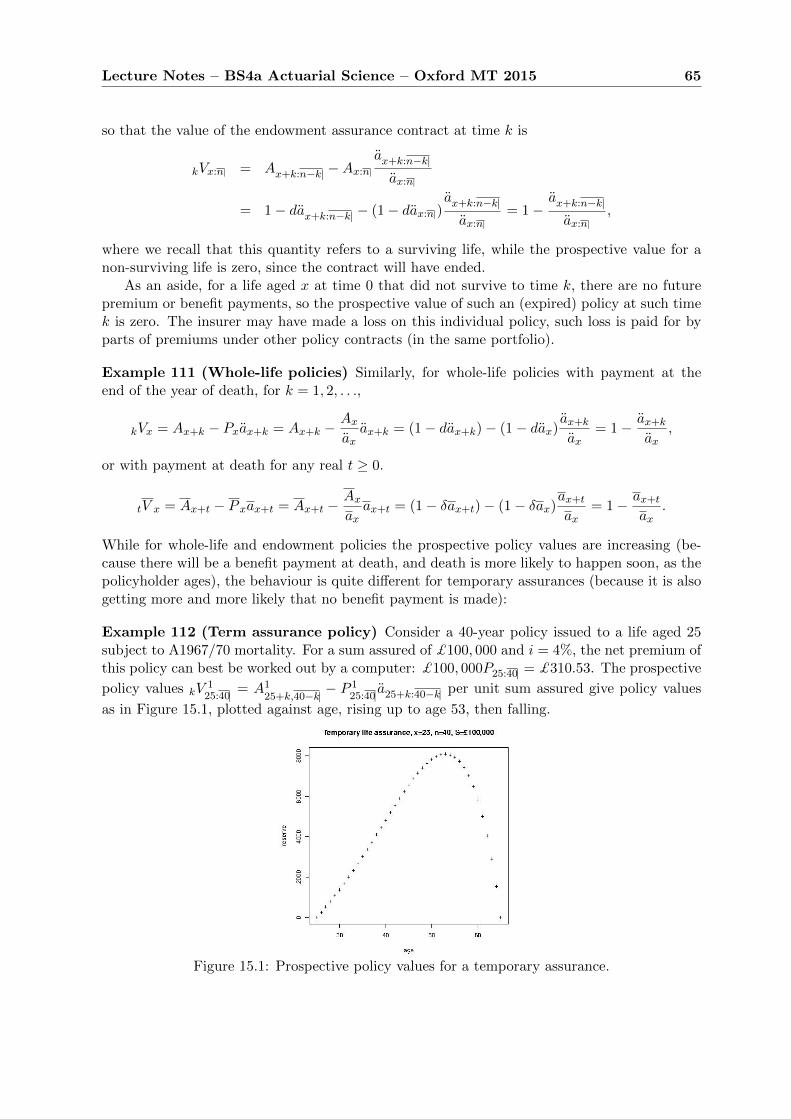
Lecture Notes – BS4a Actuarial Science – Oxford MT 2015 65
so that the value of the endowment assurance contract at time k is
kVx:n| = Ax+k:n−k| −Ax:n|ax+k:n−k|
ax:n|
= 1− dax+k:n−k| − (1− dax:n|)ax+k:n−k|
ax:n|= 1−
ax+k:n−k|
ax:n|,
where we recall that this quantity refers to a surviving life, while the prospective value for anon-surviving life is zero, since the contract will have ended.
As an aside, for a life aged x at time 0 that did not survive to time k, there are no futurepremium or benefit payments, so the prospective value of such an (expired) policy at such timek is zero. The insurer may have made a loss on this individual policy, such loss is paid for byparts of premiums under other policy contracts (in the same portfolio).
Example 111 (Whole-life policies) Similarly, for whole-life policies with payment at theend of the year of death, for k = 1, 2, . . .,
kVx = Ax+k − Pxax+k = Ax+k −Axaxax+k = (1− dax+k)− (1− dax)
ax+kax
= 1− ax+kax
,
or with payment at death for any real t ≥ 0.
tV x = Ax+t − P xax+t = Ax+t −Axaxax+t = (1− δax+t)− (1− δax)
ax+tax
= 1− ax+tax
.
While for whole-life and endowment policies the prospective policy values are increasing (be-cause there will be a benefit payment at death, and death is more likely to happen soon, as thepolicyholder ages), the behaviour is quite different for temporary assurances (because it is alsogetting more and more likely that no benefit payment is made):
Example 112 (Term assurance policy) Consider a 40-year policy issued to a life aged 25subject to A1967/70 mortality. For a sum assured of £100, 000 and i = 4%, the net premium ofthis policy can best be worked out by a computer: £100, 000P25:40| = £310.53. The prospective
policy values kV125:40| = A1
25+k,40−k| − P125:40|a25+k:40−k| per unit sum assured give policy values
as in Figure 15.1, plotted against age, rising up to age 53, then falling.
Figure 15.1: Prospective policy values for a temporary assurance.
Lecture 16
Reserves
Reading: Gerber Sections 6.1, 6.3, 6.11
In many long-term life insurance contracts the cost of benefits is increasing over the term butpremiums are level (or single). Therefore, the insurer needs to set aside part of early premiumpayments to fund a shortfall in later years of contracts. In this lecture we calculate such reserves.
16.1 Reserves and random policy values
Recall
Prospective policy value = expected time-t value of future benefits
− expected time-t value of future premiums.
If this prospective policy value is positive, the life office needs a reserve for that policy, i.e. anamount of funds held by the life office at time t in respect of that policy. Apart possibly froman initial reserve that the insurer provides for solvency reasons, such a reserve typically consistsof parts of earlier premium payments.
If the reserve exactly matches the prospective policy value and if experience is exactlyas expected in the policy basis then reserve plus future premiums will exactly meet futureliabilities. Note, however, that the mortality assumptions in the policy basis usually build astochastic model that for a single policy will produce some spread around expected values. Iflife offices hold reserves for portfolios of policies, where premiums for each policy are set tomatch expected values, randomness will mean that some policies will generate surplus that isneeded to pay for the shortfall of other policies. In practice insurers will usually reserve on aprudent (slightly cautious) basis so that aggregate future experience would have to be very badfor reserves plus future income not to cover future liabilities.
If part of the risk of very bad future experience (e.g. untimely death of a large number ofpolicy holders) is due to specific circumstances (such as acts of terrorism or war) the insurermay be able to eliminate such risk by exclusions in the policy contract or by appropriate re-insurance, where the life office passes on such risk to a re-insurance company by paying anappropriate premium from their premium income. We will get back to the notion of pooling ofinsurance policies, which is one of the essential reasons why insurance works. On a superficiallevel, re-insurance can be seen as a pooling of portfolios of insurance policies.
66
Lecture Notes – BS4a Actuarial Science – Oxford MT 2015 67
When calculating present values of insurance policies and annuity contracts in the first place,it was convenient to work with expectations of present values of random cashflows dependingon a lifetime random variable Tx or Kx = [Tx].
We can formalise prospective policy values in terms of an underlying stochastic lifetimemodel, and a constant-i (or constant-δ) interest model. A life insurance contract issued to alife aged x gives rise to a random cash flow C = CB − CP of benefit inflows CB and premiumoutflows −CP . The associated prospective policy value is
E(Lt|Tx > t), where Lt = Valt(CB|(t,∞) − C
P|[t,∞)),
where the subtlety of restricting to times (t,∞) and [t,∞), respectively, arises naturally (andwas implicit in calculations for Examples 110 and 111), because premiums are paid in advanceand benefits in arrears in the discrete model, so for t = k ∈ N, a premium payment at time kis in advance (e.g. for the year (k, k + 1]), while a benefit payment at time k is in arrears (e.g.for death in [k − 1, k)). Note, in particular, that if death occurs during [k − 1, k), then Lk = 0and Lk−1 = v − Px, where v = (1 + i)−1.
Proposition 113 (Recursive calculation of policy values) For a whole-life assurance, wehave
(kVx + Px)(1 + i) = qx+k + px+k k+1Vx.
By general reasoning, the value of the policy at time k plus the annual premium for year kpayable in advance, all accumulated to time k + 1 will give the death benefit of 1 for death inyear k+ 1, i.e., given survival to time k, a payment with expected value qx+k and, for survival,the policy value k+1Vx at time k + 1, a value with expectation px+k k+1Vx.
Proof: The most explicit actuarial proof exploits the relationships between both assurance andannuity values for consecutive ages (which are obtained by partitioning according to one-yeardeath and survival)
Ax+k = vqx+k + vpx+kAx+k+1 and ax+k = 1 + vpx+kax+k+1.
Now we obtain
kVx + Px = Ax+k − Pxax+k + Px
= vqx+k + vpx+kAx+k+1 − (1 + vpx+kax+k+1)Px + Px
= v(qx+k + px+k(Ax+k+1 − Pxax+k+1)
= v(qx+k + px+k k+1Vx).2
An alternative proof can be obtained by exploiting the premium conversion relationship,which reduces the recursive formula to ax+k = 1 + vpx+kax+k+1. However, such a proof doesnot use insight into the cash-flows underlying the insurance policy.
A probabilistic proof can be obtained using the underlying stochastic model: by definition,
kVx = E(Lk|Tx > k), but we can split the cash-flow underlying Lk as
CB|(k,∞) − CP|[k,∞) = ((0,−Px), (1, 1{k≤Tk<k+1}), C
B|(k+1,∞) − C
P|[k+1,∞)).
Taking Valk and E( · |Tx > k) then using E(1{k≤Tx<k+1}|Tx > k)=P(Tx < k+ 1|Tk > k)=qx+k,we get
kVx = −Px + vqx+k + vE(Lk+1|Tx > k) = −Px + vqx+k + vpx+k k+1Vx,
where the last equality uses E(X|A) = P(B|A)E(X|A∩B)+P(Bc|A)E(X|A∩Bc), the partitiontheorem, where here X = Lk+1 = 0 on Bc = {Tx < k + 1}.
There are similar recursive formulas for the other types of life insurance contracts.
Lecture Notes – BS4a Actuarial Science – Oxford MT 2015 68
16.2 Thiele’s differential equation
In the case of continuous time, the analogue of the recursive formula of Proposition 113 is adifferential equation. In fact, if we write that formula as
k+1Vx − kVx =1
px+k(i kVx + (1 + i)Px − qx+k(1− kVx)) ,
it describes the variation of the prospective policy value with time. The term i kVx + (1 + i)Pxjust reflects interest and premium payments, while the remainder is an adjustment for the factthat the increase is between two conditional expectations with different conditions; indeed thedenominator px+k = P(T ≥ x+ k+ 1|T ≥ x+ k) is for the extra conditioning needed for k+1Vx,while qx+k(1− kVx) is the expected change in policy value with death occurring in [k, k + 1).
With such interpretations in mind, we expect that for a policy basis
• force of interest δ,
• premiums payable continuously at rate P x per annum
• sum assured of 1 payable immediately on death
we have hpx ≈ 1 for small h > 0, and hence
t+hV x − tV x ≈ δh tV x + hP x − (1− tV x)(1− e−hµx+t).
Dividing by h and letting h ↓ 0, we should (and, by the following theorem do) get
∂
∂ttV x = δ tV x + P x − µx+t(1− tV x).
Theorem 114 (Thiele) Given a policy basis for an assurance contract for a life aged x:
• a force of interest δ(t) at time t ≥ 0,
• force of mortality µx+t at age x+ t,
• a single benefit payment of c(t) payable on death at time t ≥ 0,
• continuous premium payments at rate π(t) at times t ≥ 0,
the premiums are net premiums if∫ ∞0
π(t)v(t)tpxdt =
∫ ∞0
c(t)v(t)µx+t tpxdt, where v(t) = exp
{−∫ t
0δ(s)ds
}.
Furthermore, the prospective policy value V (t) satisfies
V′(t) = δ(t)V (t) + π(t)− µx+t(c(t)− V (t)). (1)
Proof: The first assertion follows straight from the principle of net premiums to be such thatexpected discounted premium payments equal expected discounted benefit payments; here, theformer is
E(∫ Tx
0π(t)v(t)dt
)=
∫ ∞0
π(t)v(t)E(1{Tx>t})dt =
∫ ∞0
π(t)v(t)tpxdt,
where we used E(1{Tx>t}) = P(Tx > t) = F x(t) = tpx, and the latter is
E (c(Tx)v(Tx)) =
∫ ∞0
c(t)v(t)fx(t)dt =
∫ ∞0
c(t)v(t)µx+t tpxdt,
where we used the probability density function fx(t) = µx+t tpx of Tx.For the second assertion, we note that F x+t(r) = F x(t+ r)/F x(t) and differentiate
V (t) =1
v(t)F x(t)
∫ ∞t
c(s)v(s)µx+s F x(s)ds− 1
v(t)F x(t)
∫ ∞t
π(s)v(s)F x(s)ds
using elementary differentiation
1
v(t)= exp
(∫ t
0δ(s)ds
)⇒
(1
v
)′(t) =
δ(t)
v(t),
and similarly (1/F x)′(t) = µx+t/F x(t), then applying the three-factor product rule (fgh)′ =(fg)′h+ fgh′ = f ′gh+ fg′h+ fgh′ and the Fundamental Theorem of Calculus, to get
V′(t) = (δ(t) + µx+t)V (t)− c(t)µx+t + π(t).
2
We can also interpret Thiele’s differential equation 1, as follows, in the language of a largegroup of policies: the change in expected reserve V (t) for a given surviving policy holder attime t consists of an infinitesimal increase due to the force of interest δ(t) acting on the currentreserve volume V (t), a premium inflow at rate π(t) and an outflow due to the force of mortalityµx+t acting on the shortfall c(t) − V (t) that must be met and is hence deducted from thereserve of all surviving policy holders including our given surviving policy holder. As in themodel of discrete premium/benefit cash-flows, actual reserves per policy here will fluctuatearound expected reserves discussed here because the mortality part will not act continuously,but discretely (at continuously distributed random times) when the policyholders in the groupof policies die; similarly the reserve of our given policyholder will actually drop to zero at death,the shortfall for the benefit payment being recovered from the reserves of surviving policyholdersin the group (but remember that V (t) is a conditional expectation given survival to t, so V (t)itself will never jump to zero in a model with continuously distributed lifetimes).
Appendix A
A.1 Some old exam questions
1. (i) Define and briefly discuss the concept of the yield y(c) of a cash-flow c. Quote(without proof) a general condition, in terms of positive and negative cash-flows,that ensures the existence of the yield in most practical situations.
(ii) Show that (Ia)n| =an| − nvn
i.
(iii) A special savings account pays out annual interest over 25 years at interest ratesincreasing annually by 0.25%, from 2% at the end of the first year to 8% at theend of the 25th year. The account does not allow any deposits except at the verybeginning. Also interest is not reinvested into the account. Write down the cash-flowassociated with an investment of £10,000 into the account. Show that the yield onthis account is greater than 4.44% if no withdrawals are made before the end of the25th year.
(iv) An investment project gives rise to the following cash-flows. For an initial outlay of£3,000,000, continuous income is received for 25 years at a monthly rate of £20,000.Based on a market interest rate of 4% per annum, verify that the discounted paybackperiod exists and calculate it.
2. (i) An investor is considering investing in the shares of a company. The shares paya dividend every 6 months, with the most recent dividend paid exactly 2 monthsago. This last dividend was d0, the purchase price of a single share is P and theannual effective rate of return expected from the investment is 100i%. Dividends areexpected to grow at a rate of 100g% per annum from the level of d0 where g < i.Dividends are expected to be paid in perpetuity.
(a) Show that the discounted dividend price P satisfies
P =d0(1 + i)−1/3
(1 + g)−1/2 − (1 + i)−1/2.
(b) The investor delays purchasing the shares for exactly 1 month, at which timethe price of a single share is £20 and 100g% = 3%. Given that d0 = £0.40,calculate the annual effective rate of return expected by the investor.
(ii) The same company also offers investments into their corporate bonds, which aredefault-free. These corporate bonds have a term of 10 years, pay semi-anual coupons,in arrears, of 4% per annum and are redeemable at 110% per unit nominal. Thepurchase price is such as to provide a gross rate of return of 6% per annum.
70

Exam paper 1 – BS4a Actuarial Science – Oxford MT 2015 71
(a) Show that the purchase price is £91.30 per £100 nominal.
(b) The investor buys bonds at the purchase price given in (a). He is liable to incometax at 20% and capital gains tax at 30%. Calculate his net rate of return.
Appendix B
Notation and introduction toprobability
We cannot give a full development of required probability theory here, but we shall discusssome of the main concepts by introducing our notation.
In the preceding example, the redemption payment R is to be modelled as a random variablethat can take the values 100 and 0. The important information about R is its distribution, thatis given by probabilities pR(0)+pR(100) = 1. This specification allows to derive the distributionof related random variables like S = (1 + i)−nR.
Definition 115 The distribution of a discrete random variable R is represented by its set ofpossible outcomes {rj : j ∈ N} ⊂ R (e.g. rj = j) and its probability mass function (p.m.f.)pR : R→ [0, 1] satisfying pR(r) = 0 for all r 6∈ {rj : j ∈ N} and
∑j∈N pR(rj) = 1. We write for
A ⊂ R
P (R ∈ A) =∑
j∈N:rj∈ApR(rj).
To define a multivariate discrete random variable (R1, . . . , Rn), we replace R by Rn in the abovephrases and denote the p.m.f. by p(R1,...,Rn).
72
Lecture B: Notation and introduction to probability 73
Finally, we define for functions g : {rj : j ∈ N} → R
E(g(R)) =∑j∈N
g(rj)pR(rj)
provided the series converges.
Definition 116 The distribution of a continuous random variable R is represented by its Rie-mann integrable probability density function (p.d.f.) fR : R→ [0,∞) satisfying
∫∞−∞ fR(r)dr =
1. We write for A ⊂ R
P (R ∈ A) =
∫AfR(r)dr =
∫ ∞−∞
1{r∈A}fR(r)dr.
and for functions g : Rn → R
E(g(R)) =
∫ ∞−∞
g(r)fR(r)dr
provided the Riemann integrals exist.To define multivariate continuous random variables (R1, . . . , Rn), replace R by Rn and in-
tegrals by multiple integrals, denote the p.d.f. by f(R1,...,Rn).
Definition 117 For a (discrete or continuous) random variable R we define the distributionfunction FR and the survival function FR by
FR(t) = P (R ≤ t) = P (R ∈ (−∞, t])FR(t) = P (R > t) = P (R ∈ (t,∞)) = 1− FR(t), t ∈ R.
If they exist, we define the mean µR and the variance σ2R of R as
µR = E(R) and σ2R = V ar(R) = E((R− E(R))2).
σR =√σ2R is called the standard deviation of R.
Definition 118 (Discrete or continuous) Random variables R1, . . . , Rn are said to be indepen-dent if
P ((R1, . . . , Rn) ∈ A1 × . . .×An) = P (R1 ∈ A1) . . . P (Rn ∈ An) (1)
for all A1, . . . , An ⊂ R (such that the integrals exist in the continuous case). Here P (Rj ∈Aj) = P ((R1, . . . , Rj , . . . , Rn) ∈ R× . . .×Aj × . . .×R) and we call the p.m.f. pRj or p.d.f. fRj
of Rj the marginal p.m.f. or p.d.f.
Proposition 119 R and S are independent if and only if (1) holds for all Aj = (−∞, tj ],tj ∈ R, j = 1, . . . , n, if and only if
p(R,S)(r, s) = pR(r)pS(s) or f(R,S)(r, s) = fR(r)fS(s)
for all r, s ∈ R in the respective discrete and continuous cases (for the continuous case weactually need some continuity assumptions or exceptional sets, that are irrelevant in practice.In fact p.d.f.’s are only essentially unique).

Lecture B: Notation and introduction to probability 74
In practice, the dependence structure can always be derived from a small set of independentrandom variables, and dependencies only arise when these are transformed.
Example 120 Assume, that the life time T of a light bulb has a geometric distribution withparameter q ∈ (0, 1), i.e. P (T = n) = (1 − q)qn, n = 0, 1, . . .. Then the random variablesBn = 1{T=n}, i.e. Bn = 1 if T = n and Bn = 0 if T 6= n, are Bernoulli variables with parameter(1− q)qn. Of course, the Bn are not independent, since e.g.
P (B0 = 1, B1 = 1) = P (T = 0, T = 1) = 0 6= P (B0 = 1)P (B1 = 1).
We recall that µR is the average value of R, also in the sense that
Proposition 121 (Weak law of large numbers, Tchebychev’s inequality) Given a sequenceof independent, identically distributed random variables (Rj)j≥1 with existing mean µ = µRj ,we have
P
∣∣∣∣∣∣ 1nn∑j=1
Rj − µ
∣∣∣∣∣∣ > ε
→ 0 as n→∞
for all ε > 0, i.e. P − limn→∞1n
∑nj=1Rj = µ, where P − lim denotes the limit in probability.
More precisely, if the variance σ2 = σ2Rjexists, P
∣∣∣∣∣∣ 1nn∑j=1
Rj − µ
∣∣∣∣∣∣ > ε
≤ σ2
nε2.
σ2R is a measure for the spread of the distribution of R. Its definition σ2R = E((R − µR)2)can be read as the expected (squared) deviation from the mean. Also the preceding propositionindicates that a high σ2R means more deviation from the mean.