AHybridShortestPathAlgorithmfor Intra-Regional Queries on

A Hybrid Shortest Path Algorithm for

Intra-Regional Queries on Hierarchical Networks

Gutemberg Guerra-Filho1 and Hanan Samet2!

1 Department of Computer Science and Engineering,University of Texas at Arlington,

Arlington, TX USA2 Department of Computer Science,University of Maryland, College Park

Abstract. A hierarchical approach to the single-pair shortest path prob-lem subdivides a network with n vertices into r regions with the samenumber m of vertices (n = rm) and iteratively creates higher levels ofa hierarchical network by merging a constant number c of adjacent re-gions. In a hierarchical approach, shortest paths are computed at higherlevels and expanded towards lower levels through intra-regional queries.We introduce a hybrid shortest path algorithm to perform intra-regionalqueries. This strategy uses a subsequence of pre-processed vertices thatbelong to the shortest path while actually computing the whole shortestpath. At the lowest level, the hybrid algorithm requires O(m) time andspace assuming a uniform distribution of vertices. For higher levels, thepath view approach takes O(1) time and requires O(ckm) space.

1 Introduction

Information systems that assist drivers in planning a travel are required to im-prove safety and efficiency of automobile travel. These systems use real-timetraffic information gathered by traffic control and surveillance centers like traf-fic congestion and roadwork. They aid travelers in finding the optimal path totheir destinations considering distance, time and other criteria. This helps toeliminate unnecessary travel time reducing accidents and pollution.

A Moving Object Database (MOD) is a special form of a spatial databasethat represents information about moving objects, their location in space, andtheir proximity to other entities or objects. In spatial database applications,the embedding space consists in a geographical network with a distance metricbased on shortest paths. Hence, shortest path finding is a basic operation inMODs. This operation is used as a subroutine by many other proximity queries,including nearest neighbors [10]. In particular, finding nearest neighbors in aspatial network presumes that the shortest path to the neighbors have beencomputed already. The efficiency issues related to this operation are critical to

! This work was supported in part by the National Science Foundation under GrantsIIS-10-18475, IIS-09-48548, IIS-08-12377, and CCF-08-30618.

44 G. Guerra-Filho and H. Samet

MODs due to the dynamic and real-time characteristics of such databases. Alarge number of queries in a huge network may prevent the system from meetingthe real-time requirement when a non-efficient approach is used.

A path view or transitive closure contains the information required to re-trieve a shortest path corresponding to each pair of vertices in the network. Thisstrategy pre-computes all shortest paths in the network. Once the path view iscreated, any path query is performed with a lookup in the path view and report-ing the sequence of vertices that represent the path. A path query takes O(n)time using a path view, since the number of vertices in the path may be linearin the worst case. The path view strategy requires O(n2) time for pre-processing[5, 8] and O(n2) space. The quadratic space is achieved when a predecessor ma-trix represents the path view. Methods that pre-compute and store the shortestpaths between every pair of vertices in a graph assume that the real-time com-putation of the shortest paths for large networks may not be feasible. However,the focus of their work is the compact encoding of the O(n2) shortest paths andefficient retrieval. However, a major drawback of path view approaches is thatlarge networks may need an unacceptable amount of time and space in order tosatisfy the real-time constraint.

A hierarchical approach for shortest path finding is one possible way to sat-isfy both time and space efficiency requirements for moving object databasesbased on large geographical networks. A hierarchical approach subdivides a sin-gle network into r smaller regions. Each such region has the same number m ofvertices and belongs to the lowest level of the hierarchy. The same size for regionsis a property enforced at the other levels by creating a higher level merging cadjacent regions. This process creates a hierarchy of multilevel networks for apath finding search. The parameters 〈r,m, c〉 completely define the structure ofa simple hierarchy of networks.

Given a hierarchy of networks, a hierarchical shortest path algorithm startsat the lowest level network from the source vertex. When the current regionis completely traversed, the search is promoted to the next higher level. Thepromotion step is executed once at each level until it reaches the highest level.At this point, the search is demoted to the next lower level towards the des-tination vertex. The demotion step is performed until encountering the lowestlevel network. The resulting hierarchical shortest path consists of subpaths ateach level of the network. If we seek only the shortest path cost, the hierarchicalpath cost is enough. However, when the actual path is required, the hierarchicalapproach executes shortest path queries inside individual regions, denoted hereas intra-regional queries, for each level in order to expand these subpaths to thenext lower level. These intra-regional queries are performed until the whole pathis represented by subpaths at the lowest level network.

In a hierarchical approach, the shortest subpaths found at higher levels areexpanded towards lower levels through intra-regional queries. Formally, an intra-regional shortest path query concerns the computation of a shortest path insideone region between two vertices on the border of the region. Therefore, theseintra-regional queries are an essential component of a hierarchical approach for

A Hybrid Shortest Path Algorithm 45

the computation of shortest paths in geographical networks. The subdivisionof large geographical networks is not restricted to hierarchical approaches and,consequently, intra-regional queries are used in other frameworks. As an example,the TIGER files of the U.S. Census Bureau are subdivided into counties.

In this paper, we propose a new strategy to execute intra-regional shortestpath queries at the lowest level of a hierarchical network. This strategy is basedon a hybrid shortest path algorithm that uses both a partial path view anda multiple-source shortest path algorithm. A partial path is a pre-computedsubsequence of vertices that belong to the shortest path. The partial path is usedto find a single shortest path between two vertices on the border of a region. Thenovel contribution of our paper is this new strategy for intra-regional shortestpath queries.

Using our hybrid shortest path algorithm, the time and space requirementsfor intra-regional queries at the lowest level of the hierarchical network is O(m)assuming a uniform distribution of vertices. This is an improvement comparedto the O(m1.5) space required by a path view algorithm. The time efficiency isachieved by extending a shortest path algorithm to consider pre-computed guidevertices and to visit a much smaller number of vertices in the process.

The rest of this paper is organized as follows. In Section 2, we review workrelated to intra-regional queries. Hierarchical approaches are described in Sec-tion 3. We present our hybrid shortest path algorithm in Section 4. Section 5presents our experimental results. Section 6 discusses the main contributions ofthis paper.

2 Related Work

This work is a natural progression from our prior work on building systems tosupport both feature-based queries (“Where is X happening?”) and location-based queries (“What is happening at location Y ?”) [1] as in systems such asQUILT [20] and the SAND Browser [12]. It is also applicable to surface data(e.g., [22]). Queries on road networks have received particular interest [18] withshortest path finding receiving renewed attention due to applications in spatialnetwork databases such as MapQuest, Google Maps, Yahoo! Maps, Bing Maps,and others. Among these applications, nearest neighbors algorithms [2, 3] requirethe efficient computation of shortest path distances in spatial networks. How-ever, besides these client applications, shortest path finding has been recentlyaddressed with regards to the efficient encoding of path views. Samet et al. [13–15] pre-compute the shortest paths between all possible vertices in the network.The path view is encoded by subdividing the shortest paths from a single vertexbased on the first edges of each shortest path. They further reduce the spacerequirements to store the path view by exploring spatial coherence with a short-est path quadtree. Similarly, Sankaranarayanan et al. [16, 17, 19] propose a newencoding of the path view that aggregates source and destination vertices intogroups that share common vertices or edges on the shortest paths between them.


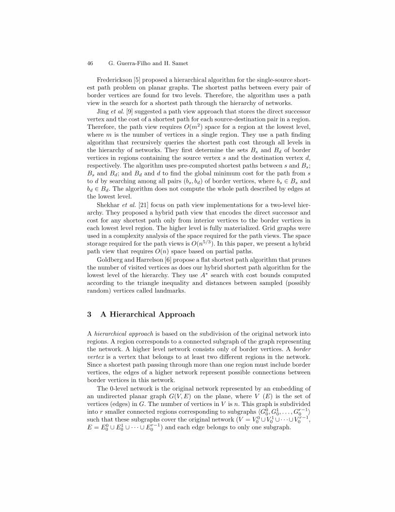
Frederickson [5] proposed a hierarchical algorithm for the single-source short-est path problem on planar graphs. The shortest paths between every pair ofborder vertices are found for two levels. Therefore, the algorithm uses a pathview in the search for a shortest path through the hierarchy of networks.

Jing et al. [9] suggested a path view approach that stores the direct successorvertex and the cost of a shortest path for each source-destination pair in a region.Therefore, the path view requires O(m2) space for a region at the lowest level,where m is the number of vertices in a single region. They use a path findingalgorithm that recursively queries the shortest path cost through all levels inthe hierarchy of networks. They first determine the sets Bs and Bd of bordervertices in regions containing the source vertex s and the destination vertex d,respectively. The algorithm uses pre-computed shortest paths between s and Bs;Bs and Bd; and Bd and d to find the global minimum cost for the path from sto d by searching among all pairs (bs, bd) of border vertices, where bs ∈ Bs andbd ∈ Bd. The algorithm does not compute the whole path described by edges atthe lowest level.

Shekhar et al. [21] focus on path view implementations for a two-level hier-archy. They proposed a hybrid path view that encodes the direct successor andcost for any shortest path only from interior vertices to the border vertices ineach lowest level region. The higher level is fully materialized. Grid graphs wereused in a complexity analysis of the space required for the path views. The spacestorage required for the path views is O(n5/3). In this paper, we present a hybridpath view that requires O(n) space based on partial paths.

Goldberg and Harrelson [6] propose a flat shortest path algorithm that prunesthe number of visited vertices as does our hybrid shortest path algorithm for thelowest level of the hierarchy. They use A∗ search with cost bounds computedaccording to the triangle inequality and distances between sampled (possiblyrandom) vertices called landmarks.

3 A Hierarchical Approach

A hierarchical approach is based on the subdivision of the original network intoregions. A region corresponds to a connected subgraph of the graph representingthe network. A higher level network consists only of border vertices. A bordervertex is a vertex that belongs to at least two different regions in the network.Since a shortest path passing through more than one region must include bordervertices, the edges of a higher network represent possible connections betweenborder vertices in this network.

The 0-level network is the original network represented by an embedding ofan undirected planar graph G(V,E) on the plane, where V (E) is the set ofvertices (edges) in G. The number of vertices in V is n. This graph is subdividedinto r smaller connected regions corresponding to subgraphs 〈G0

0, G10, . . . , G

r−10 〉

such that these subgraphs cover the original network (V = V 00 ∪V 1

0 ∪ · · ·∪V r−10 ,

E = E00 ∪E1

0 ∪ · · · ∪ Er−10 ) and each edge belongs to only one subgraph.


Each 0-level subgraph has m vertices and forms a suitable subdivision of thegraph G where boundaries of each corresponding region has a size of O(

√m)

vertices. Such suitable subdivision is obtained in O(n log n) time using a frag-mentation algorithm [5]. Goodrich [7] proposed an algorithm to find a separatordecomposition and a suitable subdivision in O(n) time.

For k > 0, the k-level network is generated from the (k − 1)-level network.A vertex v is in the k-level network if it belongs to two different (k − 1)-levelregions. Note that the k-level network has only border vertices. There is an edgeconnecting two k-level vertices in the k-level network if there is a path connectingthem in the same (k − 1)-level region. The k-level network is subdivided intoconnected k-level regions containing c adjacent (k − 1)-level regions such thateach (k − 1)-level region belongs to only one k-level region.

In a hierarchy of networks, the graph G associated with the original networkis represented by a set G0 of r subgraphs 〈G0

0, G10, . . . , G

r−10 〉. These subgraphs

correspond to regions that will be merged into higher level regions containing cregions3. This way, all regions at a particular level have about the same numberof vertices. Each subgraph is denoted by Gi

k

(

V ik , E

ik

)

, where k is the level in thehierarchy and i represents a region. The set of subgraphs representing regionsfor a k-level is denoted by Gk. The set of border vertices in a subgraph Gi

k isrepresented by Bi

k and Bk denotes the border vertex set for the k-level.PV i

k is the path view for the border vertices in Gik. The path view for the

border vertices contains the information required to retrieve a shortest path onlybetween any pair of border vertices in a k-level region i. The function PV i

k (u, v)returns the predecessor of vertex v in the shortest path from vertex u. Li

k isthe set of edges linking all pairs of border vertices that are connected by a pathin the subgraph Gi

k and Lk denotes these sets for the k-level. Each edge (u, v)iin Li

k represents a shortest path from u to v in Gik. If there is another edge

(u, v)j in Lk, then we just retain the edge with the minimum cost. The relationT in a particular k-level network represents the topological relation between k-level regions such that (i, j) ∈ T if and only if the intersection set of verticesBi,j

k = Bik ∩ Bj

k is not empty, where i and j are indices for different k-levelregions.

Lemma 1. Since the number of vertices embedded in a k-level region corre-sponding to subgraph Gi

k is O(ckm), the number of border vertices |Bk| is

O(√

ckm)

, where m is the number of vertices in a 0-level subgraph [5, 7, 11].

Lemma 2. If k > 0, the number of vertices |Vk| in a k-level subgraph Gik is

O(√

ck+1m)

and the number of edges |Ek| is O(

ckm)

.

A hierarchical shortest path algorithm creates shortest path tree layers PT+k

(for promotion) and PT−

k (for demotion) at each k-level of the hierarchy 〈G0, G1,

. . . , Gh〉 of networks, where Gk represents a level 〈G0k, G

1k, . . . , G

rk−1

k 〉 in the

3 We assume without loss of generality that r is a power of c, i.e., r = ch, where h isthe highest level in the hierarchy of networks.


hierarchy. We define a shortest path tree as a tree whose unique simple pathfrom root to any vertex represents a shortest path. A layer of a shortest pathtree is a subset of a shortest path tree contained in a particular level of thehierarchy of networks (see Fig. 1). The shortest path tree layers are computed inorder to find the hierarchical shortest path from a source vertex s to a destinationvertex d throughout all levels of the hierarchy. The algorithm uses a set S thatrepresents source vertices for a layer at a k-level, where each vertex in S isassociated with a cost.

070

071

120121

130

160

230

231

341

560

561

670

671

220

221

222

223

770771

772

340

Fig. 1. Shortest path tree layers in a network subdivided into six regions. The sourceand destination vertices are depicted with a cross inside a circle. Border vertices areshown as filled black circles. Only the regions containing the source and destinationvertices are depicted with all vertices. The other regions are shown only through bordervertices.

3.1 Expanding Subpaths in Higher Levels

A hierarchical shortest path from s to d consists of a sequence of subpaths〈P+

0 (s, v1), P+1 (v1, v2), P

+2 (v2, v3), . . . , P

+h−1

(vh−1, vh), P−

h (vh, vh+1),

P−

h−1(vh+1, vh+2), . . . , P

−2 (v2h−2, v2h−1), P

−1 (v2h−1, v2h), P

−0 (v2h, d)〉, where a

subpath from vertex vi to vertex vj in the k-level network is denoted by eitherP+k (vi, vj) or P

−

k (vi, vj). In order to have a complete shortest path, a hierarchicalalgorithm executes intra-regional queries for each k-level expanding subpaths atthe k-level to subpaths at the next lower level until the whole path consists onlyof edges in the lowest level network.

The Expand-Path algorithm given below finds a whole shortest path from s tod represented by a sequence of edges in the lowest level network. The algorithmtraverses the shortest path tree layers PT±

k in order to retrieve the subpathsthat compose a shortest path from s to d at all levels of the hierarchy. Then, the


algorithm performs intra-regional queries to expand each edge of these subpathsinto a path P at a lower level.

Algorithm Expand-Path(〈PT+0 , . . . , PT+

h−1, PT−

h , PT−

h−1, . . . , PT−

0 〉, s, d)

1. P−

0 (v2h, d)← Traverse-Backwards(

PT−

0 , d)

2. for k ← 1 to h do(a) P−

k (v2h−k, v2h−k+1) ← Traverse-Backwards(

PT−

k , v2h−k+1

)

3. for k ← h− 1 to 1 do(a) P+

k (vk, vk+1)← Traverse-Backwards(

PT+

k , vk+1

)

4. P+0 (s, v1)← Traverse-Backwards

(

PT+0 , v1

)

5. for k ← h to 1 do(a) P ← ∅(b) for u← vk ∧ (u, v)i ∈ P−

k (vk, v2h−k+1) to v2h−k+1 doi. P ← P⊕ Intra-Regional(u, v, k, i)

(c) P−

k−1(vk−1, v2h−k+2)← P+

k−1(vk−1, vk)⊕ P ⊕ P−

k−1(v2h−k+1, v2h−k+2)

Initially, the algorithm traverses each shortest path tree layer backwards us-ing the procedure Traverse-Backwards (steps 1, 2, 3, and 4). This procedurecreates the subpaths P+

k (vj , vj+1) and P−

k (vj , vj+1) at each k-level by retriev-ing a sequence of edges (u, v)i for each subpath. The algorithm expands eachsubpath starting at the highest level until it finds a whole path represented byedges only at the lowest level (step 5). For each k-level, the algorithm takes thecorresponding subpath P−

k (vk, v2h−k+1) and the procedure Intra-Regional ex-pands each edge (u, v)i in this subpath into a subpath in the (k − 1)-level (step5.b). This procedure finds the subpath from u to v in the subgraph Gi

k−1 corre-sponding to a region i at the (k−1)-level. These subpaths at the (k−1)-level areconcatenated (operator ⊕) into a path P (step 5.b.i). Then, all subpaths at the(k − 1)-level are concatenated into only one subpath P−

k−1(vk−1, v2h−k+2) (step

5.c).An important issue in the complexity analysis of the Expand-Path algorithm

is the number of edges that an expanded shortest path will have at a particularlevel of the hierarchy.

Lemma 3. The number of edges in a shortest path expanded to the (h− i)-levelis O(2i).

For intra-regional queries, we may use any flat strategy. However, we proposean efficient method for this task in the next section. A path view strategy pre-computes all shortest paths in the network for each region. When c = 2, thisstrategy requires O(m) time to retrieve a shortest path at the lowest level andO(1) time otherwise. The path view strategy requires O(m1.5) space at thelowest level and O(|Bk|2) = O(ckm) otherwise. The path view at the highestlevel and the expanded shortest path at the lowest level require O(n) space.They dominate the space requirement for Expand-Path.

Theorem 1. If the intra-regional query is implemented as a path view approach,the algorithm Expand-Path requires O(n) time.


The path view in the highest level and the expanded shortest path in thelowest level require O(n) space. They dominate the space requirement for thealgorithm Expand-Path.

Theorem 2. If the intra-regional query is implemented as a path view approach,the algorithm Expand-Path requires O(n+m1.5) space.

Another flat strategy for intra-regional queries is a single-source shortest pathalgorithm [4]. This strategy needs O(|Vk| log |Vk|+ |Ek|) time to find a shortestpath in a k-level subgraph and requires O(|Vk|+ |Ek|) space.

Theorem 3. If the intra-regional query is implemented as a single-source short-est path algorithm, the algorithm Expand-Path requires O(n logm) time.

The single-source shortest path algorithm requires space for two subgraphsat each level of the hierarchy (except the highest) and for the expanded path P .The total space required is O(n). Therefore, there is no improvement concerningspace requirement when a single-source shortest path algorithm performs intra-regional queries in a hierarchical approach.

Theorem 4. If the intra-regional query is implemented as a single-source short-est path algorithm, the algorithm Expand-Path requires O(n) space.

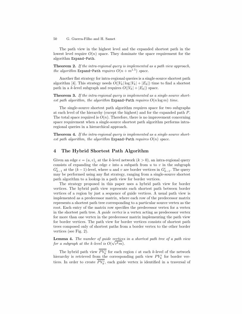
4 The Hybrid Shortest Path Algorithm

Given an edge e = (u, v)i at the k-level network (k > 0), an intra-regional queryconsists of expanding the edge e into a subpath from u to v in the subgraphGi

k−1 at the (k− 1)-level, where u and v are border vertices in Gik−1. The query

may be performed using any flat strategy, ranging from a single-source shortestpath algorithm to a lookup in a path view for border vertices.

The strategy proposed in this paper uses a hybrid path view for bordervertices. The hybrid path view represents each shortest path between bordervertices of a region by just a sequence of guide vertices. A usual path view isimplemented as a predecessor matrix, where each row of the predecessor matrixrepresents a shortest path tree corresponding to a particular source vertex as theroot. Each entry of the matrix row specifies the predecessor vertex for a vertexin the shortest path tree. A guide vertex is a vertex acting as predecessor vertexfor more than one vertex in the predecessor matrix implementing the path viewfor border vertices. The path view for border vertices consists of shortest pathtrees composed only of shortest paths from a border vertex to the other bordervertices (see Fig. 2).

Lemma 4. The number of guide vertices in a shortest path tree of a path viewfor a subgraph at the k-level is O(

√ckm).

The hybrid path view PV ik for each region i at each k-level of the network

hierarchy is retrieved from the corresponding path view PV ik for border ver-

tices. In order to create PV ik , each guide vertex is identified in a traversal of


(a) Destinations are all vertices. (b) Destinations are only border ver-tices.

Fig. 2. Shortest path tree from a source vertex (gray square) and guide vertices (blacksquares) in a lowest level region.

PV ik . A hybrid path view is implemented as a predecessor sparse matrix whose

columns only consider guide vertices V ik and border vertices Bi

k. Furthermore,the predecessor relation in this sparse matrix is only expressed in terms of guidevertices.

The algorithm Hybrid-View below creates a hybrid path view PV ik from the

path view PV ik . Each path view PV i

k is associated with a set of vertices V ik and

a set of border vertices Bik. The algorithm builds a matrix Γ to keep track of

the shortest path tree considering only paths to border vertices. The algorithmuses a vector Λ to store the number of times any vertex v ∈ V i

k is a predecessorin a particular shortest path tree of PV i

k .

Algorithm Hybrid-View(

PV ik

)

1. for u ∈ Bik do

(a) V ik ← Bi

k

(b) Λ← 0(c) Γ ← false

(d) for v ∈ Bik do

i. Γ (u, v)← true

ii. v′ ← PV ik (u, v)

iii. while v′ #= u do

A. Γ (u, v′)← true

B. v′ ← PV ik (u, v

′)(e) for v ∈ V i

k do

i. if Γ (u, v) thenA. Λ(PV i

k (u, v))← Λ(PV ik (u, v)) + 1

(f) for v ∈ V ik do

i. if Λ(v) > 1 then

A. V ik ← V i

k ∪ v

(g) for v ∈ V ik do

i. v′ ← PV ik (u, v)


ii. while v′ /∈ V ik do

A. v′ ← PV ik (u, v

′)

iii. PV ik (u, v)← v′

Hybrid-View algorithm traverses the path view PV ik computing the hybrid

path for each vertex u ∈ Bik corresponding to a shortest path tree in PV i

k .Initially, the algorithm finds the shortest path tree considering only paths toborder vertices (step 1.d). The matrix Γ identifies the edges belonging to thisshortest path tree (see Fig. 2.b). According to Γ , the algorithm computes thevector Λ that stores the number of sons for each vertex in the shortest path treeconsidering only paths to border vertices (step 1.e). Each vertex v ∈ V i

k thatis a predecessor for more than one vertex in a shortest path tree is considereda guide vertex and inserted in V i

k (step 1.f). Next, the algorithm computes the

corresponding shortest path tree only in terms of guide vertices in V ik (step 1.g).

The predecessor of a vertex in V ik is the first vertex in a backward traversal of

the corresponding shortest path tree in PV ik that belongs to V i

k .The hybrid path view computation implies pre-processing time. The time

required for the Hybrid-View algorithm is dominated by the path view scanningthat counts predecessors and finds guide vertices.

Theorem 5. Algorithm Hybrid-View needs O(m2) time at the lowest level andO((ckm)1.5) time otherwise.

The hybrid path view computation at all levels of the hierarchy requiresadditional pre-processing time O(rm2 +

∑hk=1

rck (c

km)1.5). This expression isequivalent to O(nm + n

√n) = O(n(m+

√n)). If we assume r = m =

√n, then

the additional pre-processing time becomes O(n1.5).At higher levels, a hybrid path view has the same space requirements as

a path view when c = 2. However, at the lowest level, a hybrid path viewrequires O(m) space. This is an improvement compared to the O(m1.5) spacerequired by a path view at this level. This way, the Hybrid-View algorithm spacerequirements are dominated by the path view predecessor matrix.

Theorem 6. Algorithm Hybrid-View requires O(m1.5) space at the lowest leveland O(ckm) space otherwise.

An intra-regional query for an edge (u, v)i in a 1-level network is performedby the hybrid shortest path algorithm. This algorithm uses the subgraph Gi

0

and the hybrid path view PV i0 information in order to find a single shortest

path P from u to v in the 0-level region i. PV i0 describes the shortest path

in terms of guide vertices as a partial shortest path P i0(u, v). Therefore, the

algorithm expands P i0(u, v) finding a sequence of subpaths between consecutive

guide vertices in P i0(u, v).

The algorithm Hybrid-Shortest-Path below creates a shortest path treePT whose root represents the source vertex u. A priority queue Q is used to


keep track of all information related to the current vertices in V ik−1 − PT . Each

entry (u, f(u), e) in Q represents a vertex u with an estimate cost f(u) and apredecessor edge e. The set Q′ keeps track of the vertices in Q whose cost is notinfinity and, consequently, will be reset for the next subpath search.

Algorithm Hybrid-Shortest-Path(u, v, k, i)

1. P i0(u, v)← Path-Lookup

(

PV i0 , u, v

)

2. PT ← Q← ∅3. Q← Q ∪ (u, 0, 0)4. for v′ ∈ V i

0 ∧ v′ &= u do

(a) Q← Q ∪ (v′,∞,∞)

5. for (s, d)← (u, v′) ∧ (s, d) ∈ P i0(u, v) to (v′′, v) do

(a) (u′, f(u′), e′)←Extract-Min(Q)(b) Q′ ← Q′ − u′

(c) PT ← PT ∪ (u′, f(u′), e′)(d) while u′ &= d do

i. for (u′, u′′)j ∈ Ei0

A. if f(u′) + |(u′, u′′)j | < f(u′′) then

– f(u′′)← f(u′) + |(u′, u′′)j |– e′′ ← (u′, u′′)j– Q′ ← Q′ ∪ u′′

ii. (u′, f(u′), e′)←Extract-Min(Q)iii. Q′ ← Q′ − u′

iv. PT ← PT ∪ (u′, f(u′), e′)(e) for u′ ∈ Q′ do

i. f(u′)← e′ ←∞(f) for (d, u′′)j ∈ Ei

0

i. f(u′′)← |(d, u′′)j |ii. e′′ ← (d, u′′)j

6. P ←Traverse-Backwards(PT, v)

First, the algorithm finds the partial shortest path P i0(u, v) using the proce-

dure Path-Lookup which traverses the hybrid path view PV i0 (step 1). Initially,

PT is empty and Q has all vertices with cost and predecessor edge equal to ∞,but the source vertex u whose cost is 0 (steps 2, 3, and 4). Next, the algorithmfinds a shortest subpath in Gi

0 corresponding to each edge (s, d) in the partialshortest path (step 5). The shortest subpath for each edge is computed in a sim-ilar way to Dijkstra‘s shortest path algorithm. However, the current state of thepriority queue Q means that there is no need to consider the vertices already inPT for the current subpath. Therefore, each subsequent search has an initial Qjust with all remaining vertices (step 5.e). All costs and predecessor edges are setto ∞, but vertices connected to d have its costs and predecessor edges updatedto represent that the next source vertex is d with cost equal to 0 (step 5.f). Thesubpath from u to v is computed by traversing PT from v using the procedureTraverse-Backwards (step 6).


In the worst case, the hybrid shortest path algorithm has the same timecomplexity as Dijkstra‘s single-source shortest path algorithm [4]. However, theworst case only happens when all vertices of the subgraph are visited by thealgorithm. The number of vertices visited by the hybrid shortest path algorithmis much smaller than the number of vertices of the subgraph when vertices areuniformly distributed in the region corresponding to the subgraph and the guidevertices are uniformly distributed along a shortest path (see Fig. 3).

(a) Shortest path treefor border vertices.

(b) Dijkstra’s algo-rithm.

(c) Our hybrid algo-rithm.

Fig. 3. Vertices visited by shortest path algorithms.

Theorem 7. Assume a uniform distribution of vertices at the lowest level andthe guide vertices are also uniformly distributed along a shortest path. The num-ber of vertices visited by the hybrid shortest path algorithm is O(

√m).

Assuming that vertices are uniformly distributed, the running time for thehybrid shortest path algorithm becomes O(m) at the lowest level.

Theorem 8. Assume a uniform distribution of vertices at the lowest level andthe guide vertices are also uniformly distributed along a shortest path. The hybridshortest path algorithm spends O(m) time at the lowest level.

Since the subgraph Gi0 and the hybrid path view PV i

0 are the inputs for thehybrid shortest path algorithm, the space requirements for the algorithm are thesame as for a single-source shortest path algorithm.

Theorem 9. The hybrid shortest path algorithm requires O(m) space in thek-level when k = 1 and O(ck−1m) space otherwise.

We have now seen that the best time and space requirements for intra-regional queries at the lowest level are achieved by the hybrid shortest path


algorithm. On the other hand, for higher levels, the best strategy concerningtime and space requirements is the path view approach when c = 2. Therefore,the expansion of the hierarchical path into a path with edges at the lowest levelrequires O(n) time and space.

5 Experimental Results

We evaluate the time and space performance of our hybrid approach using roadnetworks from the TIGER files of the U.S. Census Bureau. We compare ourmethod with two state-of-the-art techniques for shortest path finding on spatialnetworks: the shortest path quadtrees [13] and a flat approach based on Dijk-stra’s algorithm [4]. All algorithms were implemented using C++ in a Dell XPS730X machine with a i7 CPU at 3.20GHz and 6Gb of RAM. All data structuresnecessary for the execution of all algorithms were loaded in the main memory.

The implementation of our approach consists of four pre-processing modules:network, border, view, and hierarchy. They pre-process the TIGER/Line files inorder to find the information required by the shortest path algorithms. A roadnetwork for each county in a state is obtained in the network module. Afterthat, the border module finds for each county the set of border vertices that areshared with another county. Then, the view module computes the path view foreach county. Finally, the hierarchy module finds a higher-level network for thestate to be used in a hierarchical shortest path algorithm.

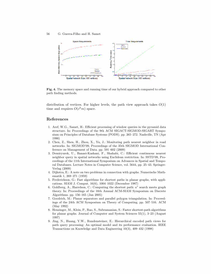
In our experimental setup, we initially selected a spatial network that re-quires only the amount of available space for all evaluated techniques. To obtainnetworks of smaller sizes, we determined the centroid of the original networkand incrementally removed vertices according to their distance to the centroid.This way, we were able to generate networks of continuous sizes to evaluate thespace requirements of all considered methods for a continuous range of networksizes. Similarly, for each network size, we compute shortest paths from the cen-troid vertex to the most distant vertex in the spatial network. This way, weinvestigated the time needed to found shortest paths of varying lengths. Thememory space and the running time obtained in our experiments is shown inFig. 4. The space requirements for our hybrid approach a virtually the same asthe requirements of the Dijkstra’s algorithm. The shortest path quadtree spendsmore space as expected from its space complexity O(n1.5). In terms of runningtime, the hybrid approach performs best followed closely by the shortest pathquadtree method.

6 Conclusion

We introduced a hybrid shortest path algorithm to perform intra-regional queries.This strategy uses a subsequence of pre-processed vertices that belong to theshortest path while actually computing the whole shortest path. At the lowestlevel, the hybrid algorithm requires O(m) time and space assuming a uniform


Fig. 4. The memory space and running time of our hybrid approach compared to otherpath finding methods.

distribution of vertices. For higher levels, the path view approach takes O(1)time and requires O(ckm) space.

References

1. Aref, W.G., Samet, H.: Efficient processing of window queries in the pyramid datastructure. In: Proceedings of the 9th ACM SIGACT-SIGMOD-SIGART Sympo-sium on Principles of Database Systems (PODS). pp. 265–272. Nashville, TN (Apr1990)

2. Chen, Z., Shen, H., Zhou, X., Yu, J.: Monitoring path nearest neighbor in roadnetworks. In: SIGMOD’09, Proceedings of the 35th SIGMOD International Con-ference on Management of Data. pp. 591–602 (2009)

3. Demiryurek, U., Banaei-Kashani, F., Shahabi, C.: Efficient continuous nearestneighbor query in spatial networks using Euclidean restriction. In: SSTD’09, Pro-ceedings of the 11th International Symposium on Advances in Spatial and Tempo-ral Databases. Lecture Notes in Computer Science, vol. 5644, pp. 25–43. Springer-Verlag (2009)

4. Dijkstra, E.: A note on two problems in connection with graphs. Numerische Math-ematik 1, 269–271 (1959)

5. Frederickson, G.: Fast algorithms for shortest paths in planar graphs, with appli-cations. SIAM J. Comput. 16(6), 1004–1022 (December 1987)

6. Goldberg, A., Harrelson, C.: Computing the shortest path: a∗ search meets graphtheory. In: Proceedings of the 16th Annual ACM-SIAM Symposium on DiscreteAlgorithms. pp. 156–165 (Jan 2005)

7. Goodrich, M.: Planar separators and parallel polygon triangulation. In: Proceed-ings of the 24th ACM Symposium on Theory of Computing. pp. 507–516. ACM(May 1992)

8. Henzinger, M., Klein, P., Rao, S., Subramanian, S.: Faster shortest-path algorithmsfor planar graphs. Journal of Computer and System Sciences 55(1), 3–23 (August1997)

9. Jing, N., Huang, Y.W., Rundensteiner, E.: Hierarchical encoded path views forpath query processing: An optimal model and its performance evaluation. IEEETransactions on Knowledge and Data Engineering 10(3), 409–432 (1998)


10. Kolahdouzan, M., Shahabi, C.: Voronoi-based k nearest neighbor search for spatialnetwork databases. In: Proceedings of the 30th International Conference on VeryLarge Databases. pp. 840–851 (2004)

11. Lipton, R., Tarjan, R.: A separator theorem for planar graphs. SIAM J. Appl.Math 36, 177–189 (1979)

12. Samet, H., Alborzi, H., Brabec, F., Esperanca, C., Hjaltason, G.R., Morgan, F.,Tanin, E.: Use of the SAND spatial browser for digital government applications.Commun. ACM 46(1), 63–66 (Jan 2003)

13. Samet, H., Sankaranarayanan, J., Alborzi, H.: Scalable network distance browsingin spatial databases. In: SIGMOD’08, Proceedings of the 2008 ACM SIGMODInternational Conference on Management of Data. pp. 43–54 (2011)

14. Sankaranarayanan, J., Alborzi, H., Samet, H.: Efficient query processing on spatialnetworks. In: Proceedings of the 13th ACM International Symposium on Advancesin Geographic Information Systems. pp. 200–209. Bremen, Germany (Nov 2005)

15. Sankaranarayanan, J., Alborzi, H., Samet, H.: Distance join queries on spatialnetworks. In: Proceedings of the 14th ACM International Symposium on Advancesin Geographic Information Systems. pp. 211–218. Arlington, VA (Nov 2006)

16. Sankaranarayanan, J., Samet, H.: Distance oracles for spatial networks. pp. 652–663. Shanghai, China (Apr 2009)

17. Sankaranarayanan, J., Samet, H.: Query processing using distance oracles for spa-tial networks 22(8), 1158–1175 (Aug 2010), best Papers of ICDE 2009 SpecialIssue

18. Sankaranarayanan, J., Samet, H.: Roads belong in databases 33(2), 4–11 (Jun2010), invited paper.

19. Sankaranarayanan, J., Samet, H., Alborzi, H.: Path oracles for spatial networks.In: Proceedings of the VLDB Endowment. pp. 1210–1221 (2009)

20. Shaffer, C.A., Samet, H., Nelson, R.C.: QUILT: a geographic information systembased on quadtrees 4(2), 103–131 (April–June 1990), also University of MarylandComputer Science Technical Report TR–1885.1, July 1987

21. Shekhar, S., Fetterer, A., Goyal, B.: Materialization trade-offs in hierarchical short-est path algorithms. In: Scholl, M., Voisard, A. (eds.) SSD’97, Proceedings of the5th International Symposium on Advances in Spatial Databases. Lecture Notes inComputer Science, vol. 1262, pp. 94–111. Springer verlag (1997)

22. Sivan, R., Samet, H.: Algorithms for constructing quadtree surface maps. In: Pro-ceedings of the 5th International Symposium on Spatial Data Handling. vol. 1, pp.361–370. Charleston, SC (Aug 1992)

Documents

AHybridShortestPathAlgorithmfor Intra-Regional Queries on