Embed Size (px)
Citation preview

From pixels to gestures: learning visual
representations for human analysis in color
and depth data sequences
A dissertation submitted by AntonioHernandez-Vela at Universitat de Barcelona tofulfil the degree of Doctor en Matematiques.
Barcelona, January 20, 2015

Director Dr. Sergio Escalera
Dept. de Matematica Aplicada i Analisi, Universitat de Barcelona &Centre de Visio per Computador
Co-director Prof. Stan Sclaroff
Dept. of Computer Science, Boston UniversityBoston, USA
Thesis Prof. Thomas Baltzer Moeslund
committee Dept. of Architecture, Design and Media Technology, Aalborg UniversityAalborg, DenmarkProf. Jordi Vitria Marca
Dept. de Matematica Aplicada i Analisi, Universitat de Barcelona &Computer Vision CenterBarcelona, SpainDr. Jordi Gonzalez Sabate
Dept. Ciencies de la Computacio, Universitat Autonoma de Barcelona &Computer Vision CenterBarcelona, Spain
International Dr. Leonid Sigal
evaluators Disney Research &Dept. of Computer Science, Carnegie Mellon UniversityPittsbutgh, USADr. Marco Pedersoli
KU LeuvenLeuven, BelgiumProf. Thomas Baltzer Moeslund
Dept. of Architecture, Design and Media Technology, Aalborg UniversityAalborg, Denmark
This document was typeset by the author using LATEX2ε.
The research described in this book was carried out at Universitat de Barcelona and theComputer Vision Center.
Copyright c© 2015 by Antonio Hernandez-Vela. All rights reserved. No part of this publi-cation may be reproduced or transmitted in any form or by any means, electronic or me-chanical, including photocopy, recording, or any information storage and retrieval system,without permission in writing from the author.
ISBN: 978-84-940902-0-2
Printed by Ediciones Graficas Rey, S.L.

A mis padres . . .

iv

Acknowledgements
The work presented in this dissertation would not have been possible without the guidanceand support of my supervisors. I am extremely thankful to my advisor Sergio Escalera for hiscontinuous efforts, dedication and encouragement during all these years. I am also gratefulto Petia Radeva, for her guidance during the early stages of my PhD. Finally, I am especiallythankful to my co-advisor Stan Sclaroff for giving me the chance to visit his research group atBoston University and having numerous conversations providing me with valuable feedbackand brilliant ideas.
During my short stay in Boston I had the great chance to meet Stan and a lot of nice andbrilliant people from the Image and Video Computing research group, from whom I learnt alot during the five months I spent at Boston University. Among them all, I must give specialthanks to Shugao and Kun for his productive conversations and brainstormings. I am alsodeeply thankful to Ramazan Gokberk and his willingness to help and share useful insightsthrough the numerous e-mail conversations we had during my days in Boston. I would alsolike to thank Tarique for making my stay in Boston a great time, I felt at home from thevery first moment.
I am also really thankful to all my colleagues from the Computer Vision Center, in specialto the people I had the great chance to meet during the Master’s academic training: Ekain,Lluıs-Pere, David, Jon and Anjan. Special thanks also to Carles, Ivet, Fran, Camp, Joan,Alejandro, Yainubis and all the people I shared a lot of precious moments with; some of youhave become really good friends.
I feel very lucky to have seen the birth of the Human Pose and Behavior Analysis(HuPBA) research group at the University of Barcelona. I am really thankful to all mycolleagues from HuPBA, in special to Miguel, Miguel Angel, Vıctor, Xavi and Albert. Notonly I learnt a lot working with you, but also shared unforgettable moments and laughs.
Muchas gracias a mis amigos de Sabadell, con ellos he pasado gran parte de mi viday momentos que nunca se olvidan. Gracias tambien a las nuevas amistades que he hechodurante estos anos desde que me mude a Barcelona; en especial a Ruben, Oroitz, Xabi, Mariay Aina.
Quiero agradecer a mis padres el apoyo y afecto que siempre me han brindado, ası comola educacion que me han dado y la paciencia que siempre han tenido conmigo durante todosestos anos. Os quiero mama y papa.
Per ultim pero no per aixo menys important, vull agraır a la Gisela el seu afecte i laseva paciencia. Em sento enormement afortunat d’haver-te conegut durant els anys d’aquestviatge. T’estimo moltıssim.
i

ii

Abstract
The visual analysis of humans from images is an important topic of interest due to itsrelevance to many computer vision applications like pedestrian detection, monitoring andsurveillance, human-computer interaction, e-health or content-based image retrieval, amongothers.
In this dissertation we are interested in learning different visual representations of thehuman body that are helpful for the visual analysis of humans in images and video sequences.To that end, we analyze both RGB and depth image modalities and address the problemfrom three different research lines, at different levels of abstraction; from pixels to gestures:human segmentation, human pose estimation and gesture recognition.
First, we show how binary segmentation (object vs. background) of the human bodyin image sequences is helpful to remove all the background clutter present in the scene.The presented method, based on Graph cuts optimization, enforces spatio-temporal consis-tency of the produced segmentation masks among consecutive frames. Secondly, we presenta framework for multi-label segmentation for obtaining much more detailed segmentationmasks: instead of just obtaining a binary representation separating the human body fromthe background, finer segmentation masks can be obtained separating the different bodyparts.
At a higher level of abstraction, we aim for a simpler yet descriptive representation ofthe human body. Human pose estimation methods usually rely on skeletal models of thehuman body, formed by segments (or rectangles) that represent the body limbs, appropriatelyconnected following the kinematic constraints of the human body. In practice, such skeletalmodels must fulfill some constraints in order to allow for efficient inference, while actuallylimiting the expressiveness of the model. In order to cope with this, we introduce a top-downapproach for predicting the position of the body parts in the model, using a mid-level partrepresentation based on Poselets.
Finally, we propose a framework for gesture recognition based on the bag of visual wordsframework. We leverage the benefits of RGB and depth image modalities by combiningmodality-specific visual vocabularies in a late fusion fashion. A new rotation-variant depthdescriptor is presented, yielding better results than other state-of-the-art descriptors. More-over, spatio-temporal pyramids are used to encode rough spatial and temporal structure. Inaddition, we present a probabilistic reformulation of Dynamic Time Warping for gesture seg-mentation in video sequences. A Gaussian-based probabilistic model of a gesture is learnt,implicitly encoding possible deformations in both spatial and time domains.
iii

iv

Resum
La analisi visual de persones a partir d’imatges es un tema de recerca molt important, deguta la rellevancia que te a una gran quantitat d’aplicacions dins la visio per computador, comper exemple: deteccio de vianants, monitoritzacio i vigilancia, interaccio persona-maquina,e-salut, o sistemes de recuperacio d’imatges a partir de contingut, entre d’altres.
En aquesta tesi volem aprendre diferents representacions visuals del cos huma, que siguinutils per a la analisi visual de persones en imatges i vıdeos. Per a tal efecte, analitzem difer-ents modalitats d’imatge com son les imatges de color RGB i les imatges de profunditat,i adrecem el problema a diferents nivells d’abstraccio, des dels pıxels fins als gestos: seg-mentacio de persones, estimacio de la pose humana i reconeixement de gestos.
Primer, mostrem com la segmentacio binaria (objecte vs. fons) del cos huma en sequenciesd’imatges ajuda a eliminar soroll pertanyent al fons de l’escena en questio. El metode presen-tat, basat en optimitzacio Graph cuts, imposa consistencia espai-temporal a les mascares desegmentacio obtingudes en frames consecutius. En segon lloc, presentem un marc metodologicper a la segmentacio multi-classe, amb la qual podem obtenir una descripcio mes detalladadel cos huma: en comptes d’obtenir una simple representacio binaria separant el cos humadel fons, podem obtenir mascares de segmentacio mes detallades, separant i categoritzantles diferents parts del cos.
A un nivell d’abstraccio mes alt, tenim com a objectiu obtenir representacions del coshuma mes simples, tot i esser suficientment descriptives. Els metodes d’estimacio de lapose humana sovint es basen en models esqueletals del cos huma, formats per segments(o rectangles) que representen les extremitats del cos, connectades unes amb altres seguintles restriccions cinematiques del cos huma. A la practica, aquests models esqueletals han decomplir certes restriccions per tal de poder aplicar metodes d’inferencia que permeten trobarla solucio optima de forma eficient, pero a la vegada aquestes restriccions suposen una granlimitacio en l’expressivitat que aquests models son capacos de capturar. Per tal de fer fronta aquest problema, proposem un enfoc top-down per a predir la posicio de les parts del cosdel model esqueletal, introduint una representacio de parts de mig nivell basada en Poselets.
Finalment, proposem un marc metodologic per al reconeixement de gestos, basat en elsbag of visual words. Aprofitem els avantatges de les imatges RGB i les imatges de profunditatcombinant vocabularis visuals especıfics per a cada modalitat, emprant late fusion. Proposemun nou descriptor per a imatges de profunditat invariant a rotacio, que millora l’estat del’art, i fem servir piramides espai-temporals per capturar certa estructura espaial i temporaldels gestos. Addicionalment, presentem una reformulacio probabilıstica del metode DynamicTime Warping per al reconeixement de gestos en sequencies d’imatges. Mes especıficament,modelem els gestos amb un model probabilistic Gaussia que implıcitament codifica possiblesdeformacions tant en el domini espaial com en el temporal.
v

vi

Contents
Acknowledgements i
Abstract iii
Resum v
1 Introduction 1
1.1 Motivation . . . . . . . . . . . . . . . . . . . . . . . . . . . . . . . . . . . . . 11.2 Objective of this thesis . . . . . . . . . . . . . . . . . . . . . . . . . . . . . . . 31.3 Contributions . . . . . . . . . . . . . . . . . . . . . . . . . . . . . . . . . . . . 41.4 Thesis outline . . . . . . . . . . . . . . . . . . . . . . . . . . . . . . . . . . . . 5
I Human body segmentation 7
2 Graph cuts optimization 11
2.1 Introduction . . . . . . . . . . . . . . . . . . . . . . . . . . . . . . . . . . . . . 112.2 Basic concepts . . . . . . . . . . . . . . . . . . . . . . . . . . . . . . . . . . . 112.3 Graph topology . . . . . . . . . . . . . . . . . . . . . . . . . . . . . . . . . . . 122.4 Energy minimization in binary problems . . . . . . . . . . . . . . . . . . . . . 12
2.4.1 Unary potential . . . . . . . . . . . . . . . . . . . . . . . . . . . . . . . 132.4.2 Pair-wise potential . . . . . . . . . . . . . . . . . . . . . . . . . . . . . 13
2.5 Multi-label generalization . . . . . . . . . . . . . . . . . . . . . . . . . . . . . 142.5.1 α-β swap . . . . . . . . . . . . . . . . . . . . . . . . . . . . . . . . . . 142.5.2 α-expansion . . . . . . . . . . . . . . . . . . . . . . . . . . . . . . . . . 15
3 Binary human segmentation 19
3.1 Introduction . . . . . . . . . . . . . . . . . . . . . . . . . . . . . . . . . . . . . 193.2 Related work . . . . . . . . . . . . . . . . . . . . . . . . . . . . . . . . . . . . 193.3 GrabCut segmentation . . . . . . . . . . . . . . . . . . . . . . . . . . . . . . . 203.4 Spatio-temporal GrabCut segmentation . . . . . . . . . . . . . . . . . . . . . 21
3.4.1 Spatial Extension . . . . . . . . . . . . . . . . . . . . . . . . . . . . . . 223.4.2 Temporal extension . . . . . . . . . . . . . . . . . . . . . . . . . . . . 22
3.5 Experiments . . . . . . . . . . . . . . . . . . . . . . . . . . . . . . . . . . . . . 233.5.1 Data . . . . . . . . . . . . . . . . . . . . . . . . . . . . . . . . . . . . . 233.5.2 Methods . . . . . . . . . . . . . . . . . . . . . . . . . . . . . . . . . . . 243.5.3 Validation measurements . . . . . . . . . . . . . . . . . . . . . . . . . 253.5.4 Spatio-Tempral GrabCut Segmentation . . . . . . . . . . . . . . . . . 26
vii

viii CONTENTS
3.5.5 Face alignment . . . . . . . . . . . . . . . . . . . . . . . . . . . . . . . 26
3.5.6 Human pose estimation . . . . . . . . . . . . . . . . . . . . . . . . . . 30
3.6 Discussion . . . . . . . . . . . . . . . . . . . . . . . . . . . . . . . . . . . . . . 34
4 Multi-label human segmentation 35
4.1 Introduction . . . . . . . . . . . . . . . . . . . . . . . . . . . . . . . . . . . . . 35
4.2 Related work . . . . . . . . . . . . . . . . . . . . . . . . . . . . . . . . . . . . 35
4.3 Method overview . . . . . . . . . . . . . . . . . . . . . . . . . . . . . . . . . . 36
4.4 Random Forests for body part recognition . . . . . . . . . . . . . . . . . . . . 37
4.5 Multi-limb human segmentation . . . . . . . . . . . . . . . . . . . . . . . . . . 40
4.6 Experiments . . . . . . . . . . . . . . . . . . . . . . . . . . . . . . . . . . . . . 41
4.6.1 Data . . . . . . . . . . . . . . . . . . . . . . . . . . . . . . . . . . . . . 42
4.6.2 Methods and validation . . . . . . . . . . . . . . . . . . . . . . . . . . 43
4.6.3 Random forest pixel-wise classification results . . . . . . . . . . . . . . 43
4.6.4 Multi-label segmentation results . . . . . . . . . . . . . . . . . . . . . 44
4.7 Discussion . . . . . . . . . . . . . . . . . . . . . . . . . . . . . . . . . . . . . . 47
II Human Pose Estimation 51
5 Detecting people: Part-based object detection 55
5.1 Introduction . . . . . . . . . . . . . . . . . . . . . . . . . . . . . . . . . . . . . 55
5.2 Pictorial structures . . . . . . . . . . . . . . . . . . . . . . . . . . . . . . . . . 56
5.2.1 Inference . . . . . . . . . . . . . . . . . . . . . . . . . . . . . . . . . . 57
5.2.2 Learning . . . . . . . . . . . . . . . . . . . . . . . . . . . . . . . . . . . 57
5.3 Deformable Part Models . . . . . . . . . . . . . . . . . . . . . . . . . . . . . . 58
5.3.1 Inference . . . . . . . . . . . . . . . . . . . . . . . . . . . . . . . . . . 59
5.3.2 Learning . . . . . . . . . . . . . . . . . . . . . . . . . . . . . . . . . . . 59
6 Contextual Rescoring for Human Pose Estimation 61
6.1 Introduction . . . . . . . . . . . . . . . . . . . . . . . . . . . . . . . . . . . . . 61
6.2 Related work . . . . . . . . . . . . . . . . . . . . . . . . . . . . . . . . . . . . 61
6.3 Method overview . . . . . . . . . . . . . . . . . . . . . . . . . . . . . . . . . . 63
6.4 Mid-level part representation . . . . . . . . . . . . . . . . . . . . . . . . . . . 64
6.4.1 Hierarchical decomposition . . . . . . . . . . . . . . . . . . . . . . . . 64
6.4.2 Poselet discovery . . . . . . . . . . . . . . . . . . . . . . . . . . . . . . 65
6.5 Contextual rescoring . . . . . . . . . . . . . . . . . . . . . . . . . . . . . . . . 66
6.6 Deformable part model formulation . . . . . . . . . . . . . . . . . . . . . . . . 68
6.7 Pictorial structure formulation . . . . . . . . . . . . . . . . . . . . . . . . . . 69
6.8 Experiments . . . . . . . . . . . . . . . . . . . . . . . . . . . . . . . . . . . . . 71
6.8.1 Data . . . . . . . . . . . . . . . . . . . . . . . . . . . . . . . . . . . . . 71
6.8.2 Methods and validation . . . . . . . . . . . . . . . . . . . . . . . . . . 72
6.8.3 Experiments with deformable part models . . . . . . . . . . . . . . . . 73
6.8.4 Experiments with pictorial structures . . . . . . . . . . . . . . . . . . 75
6.9 Discussion . . . . . . . . . . . . . . . . . . . . . . . . . . . . . . . . . . . . . . 80

CONTENTS ix
III Gesture Recognition 85
7 BoVDW for gesture recognition 89
7.1 Introduction . . . . . . . . . . . . . . . . . . . . . . . . . . . . . . . . . . . . . 897.2 Related work . . . . . . . . . . . . . . . . . . . . . . . . . . . . . . . . . . . . 907.3 Bag of Visual Words . . . . . . . . . . . . . . . . . . . . . . . . . . . . . . . . 917.4 Bag of Visual and Depth Words . . . . . . . . . . . . . . . . . . . . . . . . . . 92
7.4.1 Keypoint detection . . . . . . . . . . . . . . . . . . . . . . . . . . . . . 927.4.2 Keypoint description . . . . . . . . . . . . . . . . . . . . . . . . . . . . 927.4.3 BoVDW histogram . . . . . . . . . . . . . . . . . . . . . . . . . . . . . 947.4.4 BoVDW-based classification . . . . . . . . . . . . . . . . . . . . . . . . 94
7.5 Experiments . . . . . . . . . . . . . . . . . . . . . . . . . . . . . . . . . . . . . 957.5.1 Data . . . . . . . . . . . . . . . . . . . . . . . . . . . . . . . . . . . . . 957.5.2 Methods and validation . . . . . . . . . . . . . . . . . . . . . . . . . . 957.5.3 Results . . . . . . . . . . . . . . . . . . . . . . . . . . . . . . . . . . . 96
7.6 Discussion . . . . . . . . . . . . . . . . . . . . . . . . . . . . . . . . . . . . . . 96
8 PDTW for continuous gesture recognition 99
8.1 Introduction . . . . . . . . . . . . . . . . . . . . . . . . . . . . . . . . . . . . . 998.2 Related work . . . . . . . . . . . . . . . . . . . . . . . . . . . . . . . . . . . . 998.3 Dynamic Time Warping . . . . . . . . . . . . . . . . . . . . . . . . . . . . . . 1008.4 Handling variance with Probability-based DTW . . . . . . . . . . . . . . . . . 101
8.4.1 Distance measures . . . . . . . . . . . . . . . . . . . . . . . . . . . . . 1038.5 Experiments . . . . . . . . . . . . . . . . . . . . . . . . . . . . . . . . . . . . . 103
8.5.1 Data . . . . . . . . . . . . . . . . . . . . . . . . . . . . . . . . . . . . . 1038.5.2 Methods and validation . . . . . . . . . . . . . . . . . . . . . . . . . . 1048.5.3 Results . . . . . . . . . . . . . . . . . . . . . . . . . . . . . . . . . . . 105
8.6 Discussion . . . . . . . . . . . . . . . . . . . . . . . . . . . . . . . . . . . . . . 105
IV Epilogue 109
9 Conclusions 111
9.1 Summary of contributions . . . . . . . . . . . . . . . . . . . . . . . . . . . . . 1119.2 Final conclusions . . . . . . . . . . . . . . . . . . . . . . . . . . . . . . . . . . 1129.3 Future work . . . . . . . . . . . . . . . . . . . . . . . . . . . . . . . . . . . . . 114
A Code and Data 117
B Publications 119
Bibliography 121

x CONTENTS

List of Figures
1.1 (a) Pears are an example of objects which are simple to detect, since littlevariations can be found among different samples. (b) In contrast, articulatedobjects can suffer significant changes in their shape given their high deforma-bility, hence are harder to detect. . . . . . . . . . . . . . . . . . . . . . . . . . 2
1.2 Understanding still life scenes (a) just requires to detect the objects it iscomposed of. In contrast, understanding scenes of people (b) entail humanpose detection, facial expression recognition, or gesture recognition (in thecase of video sequences). . . . . . . . . . . . . . . . . . . . . . . . . . . . . . . 3
1.3 (a) Binary human body segmentation. (b) Multi-label human body segmen-tation. . . . . . . . . . . . . . . . . . . . . . . . . . . . . . . . . . . . . . . . . 4
1.4 Skeleton-based representations of the human body formed by (a) segments,and (b) rectangles. . . . . . . . . . . . . . . . . . . . . . . . . . . . . . . . . . 4
1.5 Gestures for letters “J” and “Z” in the American Sign Language. . . . . . . . 5
2.1 (a) Example topology of G for a typical computer vision application for 2-Dimages. (b) Example of a cut and the resulting labeling of the nodes. . . . . . 12
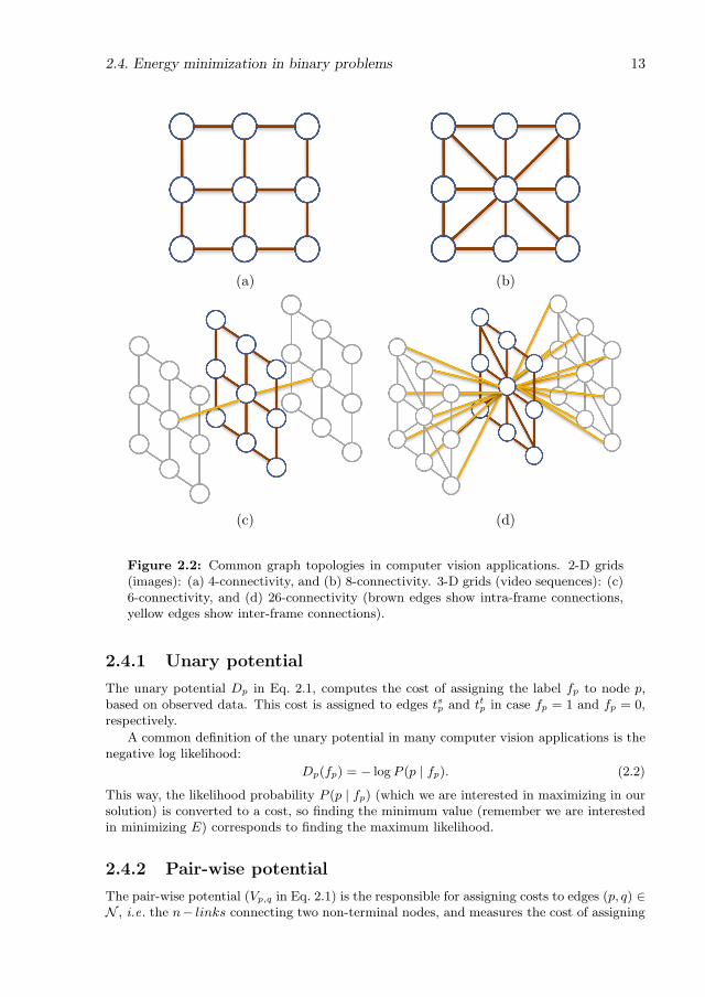
2.2 Common graph topologies in computer vision applications. 2-D grids (im-ages): (a) 4-connectivity, and (b) 8-connectivity. 3-D grids (video sequences):(c) 6-connectivity, and (d) 26-connectivity (brown edges show intra-frame con-nections, yellow edges show inter-frame connections). . . . . . . . . . . . . . . 13
2.3 Graph topology Gα for α-expansion energy minimization. Additional aribtrarynodes ap,q and respective t− links tαp are depicted in red color. . . . . . . . . 17
3.1 STGrabcut pipeline example: (a) Original frame, (b) Seed initialization, (c)GrabCut, (d) Probabilistic re-assignment, (e) Refinement and (f) Initializationmask for It+1. . . . . . . . . . . . . . . . . . . . . . . . . . . . . . . . . . . . . 23
3.2 (a) Samples of the cVSG corpus and (b) UBDataset image sequences, and (c)HumanLimb dataset. . . . . . . . . . . . . . . . . . . . . . . . . . . . . . . . . 25
3.3 From left to right: left, middle-left, frontal, middle-right and right mesh fitting. 28
3.4 Segmentation examples of (a) UBDataset sequence 1, (b) UBDataset sequence2 and (c) cVSG sequence. . . . . . . . . . . . . . . . . . . . . . . . . . . . . . 29
3.5 Samples of the segmented cVSG corpus image sequences fitting the differentAAM meshes. . . . . . . . . . . . . . . . . . . . . . . . . . . . . . . . . . . . . 29
3.6 Pose recovery results in cVSG sequence. . . . . . . . . . . . . . . . . . . . . . 31
3.7 Application of the whole framework (pose and face recovery) on an imagesequence. . . . . . . . . . . . . . . . . . . . . . . . . . . . . . . . . . . . . . . 31
xi

xii LIST OF FIGURES
3.8 Human Limb dataset results. Upper row: body pose estimation without ST-GrabCut segmentation. Lower row: body pose estimation with ST-GrabCutsegmentation. . . . . . . . . . . . . . . . . . . . . . . . . . . . . . . . . . . . 33
3.9 Application of face alignment on human body limb dataset. . . . . . . . . . 33
4.1 Pipeline of the presented method, including the input depth information, Ran-dom Forest, Graph-cuts, and the final segmentation result. . . . . . . . . . . . 38
4.2 Graph topology introducing temporal coherence. . . . . . . . . . . . . . . . . 41
4.3 Interface for semi-automatic ground-truth generation. . . . . . . . . . . . . . 42
4.4 Qualitative results; Ground Truth (a), RF inferred results (b), RWalks results(c), frame-by-frame GC results (d), and Temporally-coherent GC results (e). 46
4.5 Results from RF classification in the case of hands. First row shows theground-truth for two examples. Second row shows the RF classification re-sults. Third row shows the final α-expansion GC segmentation results. . . . . 48
4.6 Comparison of results without (a) and with (b) spatially-consistent labels. . . 48
5.1 Pedestrian detection as a classic sliding-window approach for object detection.HOG features extracted from candidate bounding boxes in the image aretested against a Linear SVM trained on images of people, which predicts apositive (green) or negative (red) answer for each candidate window. . . . . . 55
5.2 (a) Sample pictorial structure for human pose estimation; blue rectangles de-pict the different parts of the model (corresponding to parts of the humanbody) and yellow springs show the flexible connections between parts. (b)The corresponding CRF for the pictorial structure model in (a); blue nodesrepresent the parts of the model and yellow edges codify the spring-like con-nections. . . . . . . . . . . . . . . . . . . . . . . . . . . . . . . . . . . . . . . 56
5.3 Different poses of the human body. . . . . . . . . . . . . . . . . . . . . . . . . 58
6.1 Proposed pipeline for human pose estimation. Given an input image, a set ofbasic and mid-level part detections is obtained. For each basic part detectionli, a contextual representation is computed based on relations with respect tothe set of mid-level part detections. Using these contextual representations,basic part detections are rescored using a classifier for that particular basicpart class. The original and rescored detections for all basic parts are thenused in inference on a pictorial structure (PS) model to obtain the final poseestimate. . . . . . . . . . . . . . . . . . . . . . . . . . . . . . . . . . . . . . . . 63
6.2 Sample Poselet templates. Body joints are shown with colored dots, and theircorresponding estimated Gaussian distributions as blue ellipses. . . . . . . . . 64
6.3 Two sample images depicting a reference detection bounding box Bi in yellow(for the right ankle), and the set of contextual mid-level detections P in blue,orange and green for the upper body, lower body and full body, respectively. 67
6.4 Sample poselets from the LSP dataset. (a) Poselets with highest precision.(b) Poselets discovered by our selection method, maximizing precision andenforcing covering of the validation set. . . . . . . . . . . . . . . . . . . . . . 73
6.5 Qualitative results for the proposed rescoring approach incorporated in theDPM model from Yang and Ramanan [96], in the LSP dataset . . . . . . . . 74
6.6 Qualitative results for the proposed rescoring approach incorporated in theDPM model from Yang and Ramanan [96], in the PARSE dataset . . . . . . 75

LIST OF FIGURES xiii
6.7 Position prediction comparison in (a) LSP and (b) PARSE datasets. In eachplot, PCP performance is shown as a function of βu
p . We compare our proposedrescoring approach when using P = 47 poselets, automatically selected by ourproposed poselet discovery method, w.r.t. the position prediction from [69]with P = 1, 013 and P = 47 poselets. . . . . . . . . . . . . . . . . . . . . . . . 76
6.8 Comparison of different mid-level representations in (a) LSP and (b) PARSEdatasets. In each plot, PCP performance is shown as a function of βu
p . Wecompare our poselet selection maximizing precision and enforcing coveringagainst (1) the manual hierarchical decomposition from [69], (2) selecting theposelets with maximum precision, and (3) the poselet selection greedy methodfrom [15]. . . . . . . . . . . . . . . . . . . . . . . . . . . . . . . . . . . . . . . 77
6.9 Failure cases in (a) LSP and (b) PARSE datasets. Our proposed methodcannot recover the human pose correctly, mainly due to upside-down posesand cases with extra people close to the actual subject. . . . . . . . . . . . . 80
6.10 Contextual feature selection histograms computed from the learnt decisiontrees qθ , grouped by subsets of joints: (a) upper-body limbs, (b) lower-bodylimbs, (c) head & torso, and (d) full body. . . . . . . . . . . . . . . . . . . . . 81
6.11 Qualitative results on LSP dataset. (a) Gaussian-shaped position predictionfrom [69], (b) Estimated pose from [69] (just predicting position), (c) Esti-mated pose from [69] (full model), (d) Position prediction with our proposedrescoring, and (e) Our results. White crosses in columns (a) and (d) show thepart being rescored in each case; from the first row to the last one: rightmostankle, rightmost wrist, leftmost ankle, leftmost wrist. . . . . . . . . . . . . . . 82
6.12 Qualitative results on PARSE dataset. (a) Gaussian-shaped position predic-tion from [69], (b) Estimated pose from [69] (just predicting position), (c)Estimated pose from [69] (full model), (d) Position prediction with our pro-posed rescoring, and (e) Our results. White crosses in columns (a) and (d)show the part being rescored in each case; from the first row to the last one:right ankle, right wrist, right ankle, left ankle. . . . . . . . . . . . . . . . . . . 83
7.1 (a) An example of the bag of words representation for text classification. (b)Bag of visual words representation for image categorization. . . . . . . . . . . 92
7.2 BoVDW approach in a Human Gesture Recognition scenario. Interest pointsin RGB and depth images are depicted as circles. Circles indicate the assign-ment to a visual word in the shown histogram – computed over one spatio-temporal bin. Limits of the bins from the spatio-temporal pyramids decom-position are represented by dashed lines in blue and green, respectively. Adetailed view of the normals of the depth image is shown in the upper-leftcorner. . . . . . . . . . . . . . . . . . . . . . . . . . . . . . . . . . . . . . . . . 93
7.3 (a) Point cloud of a face and the projection of its normal vectors onto theplane Pxy, orthogonal to the viewing axis z. (b) VFHCRH descriptor: Con-catenation of VFH and CRH histograms resulting in 400 total bins . . . . . . 94
7.4 Confusion matrices for gesture recognition in each one of the 20 developmentbatches. . . . . . . . . . . . . . . . . . . . . . . . . . . . . . . . . . . . . . . . 97
8.1 Flowchart of the Probabilistic DTW gesture segmentation methodology. . . . 101

xiv LIST OF FIGURES
8.2 (a) Different sequences of a certain gesture category and the median lengthsequence. (b) Alignment of all sequences with the median length sequence bymeans of Euclidean DTW. (c) Warped sequences set S from which each set oft-th elements among all sequences are modelled. (d) Gaussian Mixture Modellearning with 3 components. . . . . . . . . . . . . . . . . . . . . . . . . . . . . 102
8.3 Examples of idle gesture detection on the Chalearn data set using the probability-based DTW approach. The line below each pair of depth and RGB imagesrepresents the detection of a idle gesture (step up: beginning of idle gesture,step down: end) . . . . . . . . . . . . . . . . . . . . . . . . . . . . . . . . . . 106
A.1 Human Limb dataset labels description. . . . . . . . . . . . . . . . . . . . . . 118

List of Tables
1.1 Symbols and conventions for chapters 2- 4 . . . . . . . . . . . . . . . . . . . . 9
2.1 Weights of edges Eαβ in Gαβ. . . . . . . . . . . . . . . . . . . . . . . . . . . . 152.2 Weights of edges Eα in Gα. . . . . . . . . . . . . . . . . . . . . . . . . . . . . . 17
3.1 GrabCut and ST-GrabCut Segmentation results on cVSG corpus. . . . . . . . 263.2 AAM mesh fitting on original images and segmented images of the cVSG corpus. 303.3 Face pose percentages on the cVSG corpus. . . . . . . . . . . . . . . . . . . . 303.4 Pose estimation results: overlapping of body limbs based on ground truth
masks. . . . . . . . . . . . . . . . . . . . . . . . . . . . . . . . . . . . . . . . . 313.5 Overlapping percentages between body parts (intersection over union), wins
(comparing the highest overlapping with and without segmentation), andmatching (considering only overlapping greater than 0.6). ∗ STGrabCut wasused without taking into account temporal information. . . . . . . . . . . . . 32
4.1 Average per class accuracy in % calculated over the test samples in a 5-foldcross validation. ψθ represents features of the depth comparison type fromEq. (4.1), while ψθ - the gradient comparison feature from Eq. (4.13). Omax
is the upper limit of the u and v offsets, and dmax stands for the maximaldepth level of the decision trees. . . . . . . . . . . . . . . . . . . . . . . . . . 44
4.2 Average per class accuracy in % obtained when applying the different GCapproaches –TC: Temporally coherent, Fbf: Frame-by-Frame– , and the bestresults from the RF probabilities [79] and the RWalks segmentation algorithm[44], in the first and second rows, respectively. . . . . . . . . . . . . . . . . . . 45
4.3 Symbols and conventions for chapters 5- 6 . . . . . . . . . . . . . . . . . . . . 53
6.1 List of contextual features included in cBi,Bp . For clarification, the detectionscore is encoded classwise in a sparse vector, i.e. a vector of size P set tozeros except the position corresponding to the class of the detection, whichcontains the detection score. . . . . . . . . . . . . . . . . . . . . . . . . . . . . 68
6.2 Pose estimation results for LSP dataset. The table shows the PCP for eachpart separately, as well as the mean PCP. Columns with two values indicatethe PCP for the left and right parts, respectively. The methods in the tableare grouped according to the features they use, namely: HOG (H), HOG +RGB (HC) and Shape context (SC). We compare our rescoring proposal andmid-level image representation computed with our proposed poselet selectionmethod, against the state of the art. ∗ They use extra 11, 000 images fortraining. ⋄ 14 parts. † (P = 1, 013). ‡ (P = 47, pred-pos only). . . . . . . . . 78
xv

xvi LIST OF TABLES
6.3 Pose estimation results for PARSE dataset. See Table 6.2 for table legend.*They use extra 11, 000 images for training. ⋄ 14 parts. † (P = 1, 013). ‡(P = 47, pred-pos only). . . . . . . . . . . . . . . . . . . . . . . . . . . . . . . 79
6.4 Running time (in seconds) of the test pipelines from [69] (Algorithm 8) andour proposal (Algorithm 9). . . . . . . . . . . . . . . . . . . . . . . . . . . . . 81
6.5 Symbols and conventions for chapters 7- 8 . . . . . . . . . . . . . . . . . . . . 87
7.1 Mean Levenshtein distance for RGB and depth descriptors. . . . . . . . . . . 967.2 Mean Levenshtein Distance of the best RGB and depth descriptors separately,
as well as the 2-fold and 3-fold late fusion of them. Results obtained by thebaseline from the ChaLearn challenge are also shown. Rows 1 to 20 representthe different batches.. . . . . . . . . . . . . . . . . . . . . . . . . . . . . . . . . . . . . . . . . . . . 98
8.1 Overlapping and accuracy results. . . . . . . . . . . . . . . . . . . . . . . . . . 105

Chapter 1
Introduction
1.1 Motivation
In the quest for artificial intelligence, the ultimate goal could be envisioned as the creation of“intelligent” robots, i.e. robots which have an “intelligent” behavior, following the guidelinesof our human intelligence. This intelligence can be defined in many different ways, dependingon the different processes that take place in our brains in order to perform a certain task.Among them all, it has been proven that visual intelligence –the reasoning processes relatedto our visual system– plays an important role in our global intelligent behavior, and thisfact can be easily illustrated by imagining ourselves performing daily tasks like commutingor even preparing breakfast without perceiving and processing visual information.
Visual intelligence can be defined as understanding the 3-D spatial world that surroundsus from 2-D projections of it, i.e. images, captured by our retinae. While we are not aware ofit, our brain is constantly processing visual information in order to understand our environ-ment, and it is pretty good at it, though it is a really challenging task. In our daily lives weare generally able to recognize objects, people and faces without much trouble, even thoughour 3-D world is full of objects that occlude each other and we are able to infer it fromjust 2-D projections. Moreover, we are able to recognize objects under different viewpointsor projections, usually implying a change in their appearance. However, when trying toaccomplish these tasks artificially by means of computers, we realize the challenging natureof the problem and the power of our brains.
Computer vision is the field of Artificial Intelligence dedicated to the acquisition andprocessing of images, trying to replicate the human visual intelligence using computer soft-ware and hardware. Visual tasks like object recognition have been vastly researched duringmany years and they are still a challenge for researchers in the field. The main problems toface when designing algorithms for object recognition are: changes in illumination, changesin viewpoint, presence of occlusions or object class variability, among others. While someobjects may have little appearance variations in size, color or shape things get complicatedin the case of articulated objects composed by movable parts (see Fig. 1.1). Such deformableobjects can eventually change their shape appearance considerably, thus complicating theprocess of learning patterns of their appearance.
Besides object detection and recognition, people detection has caught the attention ofmany researchers, because of its multiple applications, e.g . pedestrian detection, monitoringand surveillance, human-computer interaction e-health, or content-based image retrieval.Detecting people in images is challenging, in the first place, due to the the articulated
1

2 INTRODUCTION
(a)
(b)
Figure 1.1: (a) Pears are an example of objects which are simple to detect, sincelittle variations can be found among different samples. (b) In contrast, articulatedobjects can suffer significant changes in their shape given their high deformability,hence are harder to detect.
nature of the human body: people can adopt a wide range of poses and consequently, thebody shape has a large variability. Not only that, but certain poses may also incur in self-occlusions of some body parts, thus making it more difficult to detect. In addition, differentclothing can also result in slight changes in the shape of the body, plus a significant changein color appearance. Finally, humans are animated entities that are able to perform differentactions with different purposes in comparison with static objects. Therefore, understandingimages of people is much more complicated, since human behavior or social signal come intoplay (see Fig. 1.2).
In contrast to common RGB images used in Computer Vision, range images (a.k.a. depthimages) provide additional information about the 3-D world, allowing to capture the depthinformation of each pixel in the image, i.e. we know the distance from the camera sensor topoints in the scene. Therefore, range images provide a 2.5-D projection of the real world,in contrast to the 2-D projections of common RGB images, allowing for more robust objectdetection methodologies due to the richer description of the scenes and other additionalproperties like invariance to changes in illumination, for example. The main issue withrange imaging is sensor device technologies like Time-of-flight are very expensive, so accessto this kind of cameras is budget-limited. However, the release of low-cost consumer depthcameras like the Kinect from Microsoft in late 2010, supposed an affordable range imagingsolution, and many researchers in computer vision made contributions based on multi-modalRGBD (RGB plus Depth) data. As a consequence, a lot of progress has been done in thecomputer vision community during the past few years, especially in the fields of human

1.2. Objective of this thesis 3
(a) (b)
Figure 1.2: Understanding still life scenes (a) just requires to detect the objects itis composed of. In contrast, understanding scenes of people (b) entail human posedetection, facial expression recognition, or gesture recognition (in the case of videosequences).
pose estimation and gesture recognition for human-computer interaction. Nevertheless, suchlow-cost range imaging solutions still present some issues in outdoor applications, renderingthem almost useless in those cases, in front of RGB cameras.
1.2 Objective of this thesis
In this thesis, we are interested in learning different visual representations of the humanbody that are helpful for the visual analysis of humans in images and video sequences. Tothat end, we analyze both RGB and depth image modalities and address the problem fromthree different research lines, at different levels of abstraction; from pixels to gestures:
1. Human body segmentation: At the lowest level of abstraction, we consider segmen-tation in order to obtain a pixel-wise representation of the human body. Segmentationmethods aim to partition an image in different segments, usually containing differentobjects or classes of interest. On one hand, we consider binary segmentation (objectvs. background) as a pre-processing step in order to remove all the background clutter.After that, further techniques for a deeper analysis of the human body (e.g . humanpose estimation) can be applied in much smaller image regions of interest, where theactual body is located. On the other hand, multi-label segmentation methods canbe also applied for a much more detailed pixel categorization; instead of just obtian-ing a binary representation separating the human body from the background, finersegmentation masks can be obtained separating the different body parts (see Fig 1.3).
2. Human pose estimation: At a higher level of abstraction, we aim for a simpleryet descriptive representation of the human body. Human pose estimation methodsusually rely on skeletal models of the human body, formed by segments (or rectan-gles) that represent the body limbs, appropriately connected following the kinematicconstraints of the human body (see Fig. 1.4). Estimating the pose of a person is thenformulated as inferring the 2-D or 3-D position and orientation of the body limbs. Thisinformation can be then used as an intermediate image descriptor for higher-level se-mantic reasoning about the actions or activities being performed by the subjects inthe image.

4 INTRODUCTION
(a) (b)
Figure 1.3: (a) Binary human body segmentation. (b) Multi-label human bodysegmentation.
(a) (b)
Figure 1.4: Skeleton-based representations of the human body formed by (a) seg-ments, and (b) rectangles.
3. Gesture recognition: A deeper analysis and understanding of human behavior fromvisual information, usually requires to take into account the temporal dimension, i.e. toprocess video sequences instead of just still images. Topics like gesture recognition aimto detect specific motion patterns outlined by different body parts along time. Usually,these motion patterns have to be put in correspondence with finer-grained spatialconfigurations of the body parts, e.g . the hands, in order to detect complex gestureslike in sign language (see Fig. 1.5), for example. Furthermore, gesture recognition canbe used for recognizing higher-level semantic units related to human behavior, e.g .human activity recognition.
1.3 Contributions
We summarize the contributions of this thesis in the following list, classified by the corre-sponding research line:
Human body segmentation

1.4. Thesis outline 5
Figure 1.5: Gestures for letters “J” and “Z” in the American Sign Language.
• We propose a fully-automatic method for binary segmentation of people (i.e. segment-ing the human body from the background) appearing in video sequences. Our pro-posed method extends the formulation of GrabCut to video sequences, incorporatingspatio-temporal consistency by means of Mean Shift clustering (spatial consistency)and a mask initialization algorithm that enforces smooth changes between consecutiveframes (temporal consistency).
• We present a generic framework for spatio-temporally consistent multi-label objectsegmentation based on Random Forest classification and Graph-cuts theory. Thepresented methodology is applied to human limb segmentation in depth data, yield-ing a more detailed segmentation of the human body compared to a simple fore-ground/background mask.
Human pose estimation
• We propose a contextual rescoring methodology for predicting the position of bodyparts in a human pose estimation framework based on pictorial structures. This rescor-ing approach encodes high-order body part dependencies by means of a mid-level partrepresentation, yielding more confident position predictions of the body parts whilekeeping a tree-structured CRF topology in the pictorial structure framework.
• We propose an algorithm for the fully-automatic discovery of a compact contextualmid-level part representation based on Poselets. This contextual representation isable to capture pose-related information that is exploited by our proposed contextualrescoring methodology for human pose estimation.
Gesture recognition
• We propose a framework for gesture recognition based on the bag of visual wordsframework. We leverage the benefits of RGB and depth image modalities by combiningmodality-specific visual vocabularies in a late fusion fashion. A new rotation-variantdepth descriptor is presented, yielding better results than other state-of-the-art de-scriptors. Moreover, spatio-temporal pyramids are used to encode rough spatial andtemporal structure.
• We present a probabilistic reformulation of Dynamic Time Warping for gesture seg-mentation in video sequences. A Gaussian-based probabilistic model of an idle gestureis learnt, implicitly encoding possible deformations in both spatial and time domains.
1.4 Thesis outline
This thesis is divided in three self-contained main parts, one for each of the three linesof research we followed: Human body segmentation, Human pose estimation, and Gesture

6 INTRODUCTION
recognition. For the reader’s convenience, the symbol notation of each part is summarizedin a table at the beginning of each part. Given the multidisciplinary nature of this thesis,most of the chapters are structured in a similar way, including an introduction, then present-ing related work, method formulation, experimental section and a final discussion sectionsummarizing the contributions.
In Part I, we start in chapter 2 by introducing the basis of Graph cuts optimization forboth the binary case and its multi-label generalization, used in the following chapters. Inchapter 3 we present a method for binary segmentation of subjects in video sequences usinggraph cuts theory. Finally, in chapter 4 we take advantage of the multi-label generalizationof the graph cuts framework to present a methodology for multi-limb segmentation of upperbodies in multi-modal video sequences including RGB and depth data.
Part II is dedicated to Human Pose Estimation. Chapter 5 introduces two widely usedframeworks for articulated object detection and consequently, for the problem of humanpose estimation: deformable part models and pictorial structures. In chapter 6 we present acontextual rescoring method for obtaining more robust part detections in part-based objectdetection frameworks like those introduced in chapter 5.
Part III contains our contributions in Gesture Recognition. In chapter 7 we present a Bag-of-Visual-and-Depth-Words representation for gesture recognition in multi-modal RGBDdata sequences. In Chapter 8 we propose an extension of Dynamic Time Warping by defininga distance metric based on a probabilistic formulation.
Finally, conclusions and contributions of the thesis are summarized in chapter 9, as wellas future lines of research.
In the appendices we present the list of contributions resulting from the work presented inthis thesis. We first present the codes and datasets made publicly available to the community.Finally, we list the publications regarding the content of this thesis.

Part I
Human body segmentation
7


Symbol notation in Part I
Table 1.1: Symbols and conventions for chapters 2- 4
G =< V, E > Graph formed by a set of nodes V and a set of edges EP Set of non-terminal nodes
s, t Set of terminal nodes: source s and sink tN Set of non-terminal edges
T = tsp, ttp | p ∈ P Set of terminal links
C = Ps,Pt A cut on G: a binary partition of nodes P into Ps,Pt
L Set of labelsf = fp | p ∈ P Labeling of non-terminal nodes P
E Energy functionD Unary potential in EV Pair-wise potential in E
α, β, γ Random labels
I Imagez Array of pixels in I
zi = (xi, yi, Ri, Gi, Bi) Pixel information: spatial coordinates (xi, yi) and color compo-nents Ri, Gi, Bi
N Number of pixels in IT = TF , TB , TU GrabCut trimap
θ = π, µ, σ GMM parameters: mixing weights, mean and covariance matrixk Array of pixel GMM component assignmentsβ Statistics of boundaries in IΓ Pair-wise potential weight.
I = It | t = 1, ...,M Video sequenceM Number of frames in the video sequence IB Bounding box around the detected personR Central subregion of B
hskin Skin color modelδ(zi, hskin) Function that returns a subset of pixels with high likelihood
P (hskin | zi)mh Mean-shift modesF Image segmentation maskSTe Structuring elementO Overlapping factor
g Texture vectorµg , σ
2s Mean and variance of elements of g
9

10
x Mean shapeg Mean texture
Qs,Qg Matrices designing modes of variationX A shape in the image
St(x) Similarity transformationE Fitting error
ℑF ,ℑR,ℑL Face meshes for frontal, right lateral and left lateral views
L = li | i = 1, ..., P Configuration of body parts lili = (x, y, o) Parametrization of part li: postion (x, y) and orientation o
Υ Unary potential in energy function for human pose estimationΨ Pair-wise potential in energy function for human pose estimation
λ ∈ Λ Random tree in random forest Λψθ(zi) Depth comparison feature for pixel zi
θ = (u, v) A pair of offsetsΦ Set of node splitting criteria φ = (θ, τ )τ Threshold on ψθ
Z Set of random training pixels to train λZL, ZR Subsets of pixels resulting from a splitting node in λG(·) Information gain functionH(·) Entropy function
Pλ(c | zi) Probability density function stored at the leafs of λ, c ∈ Ldmax Averaged maximum depth level of trees in ΛOmax Upper limit for the module of offset θ
Ω1(fi, fj),Ω2(fi, fj) Label cost functions between labels fi, fjrsc Friedman relative ranking for strategy s and label c ∈ LRs Friedman mean ranking for strategy sk Number of strategies for Friedman testNF Number of experiments for Friedman test

Chapter 2
Graph cuts optimization
2.1 Introduction
Graph cuts optimization has been extensively used in different Computer Vision applicationslike image segmentation, image restoration, stereo matching, or any other problem that canbe formulated as an energy minimization problem [17, 20]. Graph cuts are able to find theoptimal solution (the one with minimum energy) in the case of binary problems, and near-optimal approximate solutions in the multi-label case, as long as the defined energy functionsatisfies some conditions.
In this chapter we review the theory behind Graph cuts optimization and its properties,which will be later applied in chapters 3- 4 for segmenting the human body.
2.2 Basic concepts
Let G =< V, E > be a graph formed by a set of nodes V and a set of edges E connecting them.The set of nodes V = s, t ∪ P can be decomposed in two subsets. On one hand, we notethe terminal nodes s (source) and t (sink) (light-blue-filled nodes in Fig. 2.1(a)). On theother, we denote by P the set of non-terminal nodes (dark-blue-lined nodes in Fig. 2.1(a)).
The edges E = N ∪T can be also divided in two classes. We first denote by N = (p, q) ∈E | p, q ∈ P the set of edges connecting two non-terminal nodes, also referred to as n− links(see brown-colored edges in Fig. 2.1(a)). Secondly, we consider the set of t− links, i.e. thelinks connecting a non-terminal node with the terminal nodes s and t: T = tsp, t
tp | p ∈ P,
where tsp = (s, p), ttp = (p, t) (black-colored edges in Fig 2.1(a)). Finally, every other edge inthe graph is assigned a cost, defined by the energy function that we want to minimize.
A “cut” C = Ps,Pt of the graph G is a partitioning of the nodes P into two disjointsubsets Ps and Pt, named after the terminal nodes s (source) and t (sink), respectively.Therefore, a cut unequivocally assigns each node p ∈ P to one of the t − links, producinga labelling f = fp | p ∈ P, where fp ∈ L (L = 0, 1 for the binary case). The cost of acut C is then defined as the sum of the costs of edges E in the graph G. An example of a cutis shown as an orange dotted line in Fig. 2.1(b), and the corresponding partitioning of thenodes in green and purple colors.
11

12 GRAPH CUTS OPTIMIZATION
(a) (b)
Figure 2.1: (a) Example topology of G for a typical computer vision application for2-D images. (b) Example of a cut and the resulting labeling of the nodes.
2.3 Graph topology
In computer vision applications, typical topologies for G are in the shape of N-D grids, beingN = 2 the most common case, arranging the nodes in the graph following the 2-D lattice ofan image (see Fig. 2.1). Given two contiguous pixels i and j in an image I , nodes p, q ∈ Prepresent them in the graph, and an edge (p, q) ∈ N represents their neighborhood property.Similarly, we can imagine a 3-D grid topology in order to process spatio-temporal volumesi.e. video sequences.
Different neighboring patterns can be considering to give shape to the N-D grid topolo-gies. The most popular neighborhood patterns in the case of 2-D lattices, are the 4-connectivity and the 8-connectivity. While the former just considers two nodes to be con-tiguous if they share either the x or the y coordinates (see Fig. 2.1(a-b)), the latter alsoconsiders nodes placed in the diagonals. Similarly, typical neighborhood systems in a 3-Dgrid are 6-connectivity or 26-connectivity (see Fig. 2.1(c-d)).
2.4 Energy minimization in binary problems
The min − cut/max − flow algorithm is able to efficiently find the exact solution f withminimum energy, as long as the problem is binary (L = 0, 1), and the potentials in thedefined energy function are of order 2 at most. In other words, only functions which can beexpressed as a sum of functions that take into account at most 2 variables at a time, areallowed. The standard form of such energy functions E is:
E(f) =∑
p∈P
Dp(fp) +∑
(p,q)∈N
Vp,q(fp, fq), (2.1)
where termsDp(fp) and Vp,q are “unary potential”and the “pair-wise potential”, respectively.
2.4. Energy minimization in binary problems 13
(a) (b)
(c) (d)
Figure 2.2: Common graph topologies in computer vision applications. 2-D grids(images): (a) 4-connectivity, and (b) 8-connectivity. 3-D grids (video sequences): (c)6-connectivity, and (d) 26-connectivity (brown edges show intra-frame connections,yellow edges show inter-frame connections).
2.4.1 Unary potential
The unary potential Dp in Eq. 2.1, computes the cost of assigning the label fp to node p,based on observed data. This cost is assigned to edges tsp and ttp in case fp = 1 and fp = 0,respectively.
A common definition of the unary potential in many computer vision applications is thenegative log likelihood:
Dp(fp) = − logP (p | fp). (2.2)
This way, the likelihood probability P (p | fp) (which we are interested in maximizing in oursolution) is converted to a cost, so finding the minimum value (remember we are interestedin minimizing E) corresponds to finding the maximum likelihood.
2.4.2 Pair-wise potential
The pair-wise potential (Vp,q in Eq. 2.1) is the responsible for assigning costs to edges (p, q) ∈N , i.e. the n− links connecting two non-terminal nodes, and measures the cost of assigning

14 GRAPH CUTS OPTIMIZATION
labels fp, fq to contiguous nodes p, q, based on observed data like in the case of the unarypotential. This pair-wise potential is meant to enforce “smoothness” in the solution, fosteringsimilar pixels to have the same label. Therefore, Vp,q is meant to be a non-convex functionof |fp − fq |, i.e. a discontinuity-preserving function.
An important and widely used example for such discontinuity-preserving function is thePotts model:
Vp,q(fp, fq) = [fp 6= fq ], (2.3)
where [χ] is an indicator function that takes the value 1 if condition χ is satisfied, or 0otherwise. Therefore, this model encourages solutions consisting on different regions suchthat pixels in the same region are assigned the same label.
2.5 Multi-label generalization
Although graph cuts optimization is inherently binary, the same framework has been alsoextended to multi-label problems 1, i.e. when |L| > 2. The generalization of a binary cutC = S , T to a multi-label case can be then formulated as a partitioning P = Pl | l ∈ L,where Pl = p ∈ P | fp = l.
Given that |L| > 2, the number of label combinations in the boundaries of a possible cutC can be much higher (it grows quadratically on |L|). Hence, more interesting versions ofthe Potts model can be taken into consideration where different values can be assigned todifferent pairs of labels α, β ∈ L.
Exact multi-label optimization is only possible when labels L can be linearly ordered, andthe pair-wise potential is defined as a specific convex function Vp,q = |fp−fq|, but in practicefor computer vision applications, the obtained result is oversmoothed. However, there aremore interesting algorithms that get approximate solutions: α-β swap and α-expansion. Wereview them in the following subsections.
2.5.1 α-β swap
This algorithm is able to find an approximate solution (without any guarantee of closenessto the optimal solution), as long as the pair-wise potential satisfies the following conditionsfor any pair of labels α, β ∈ L:
V (β, α) = V (α, β) ≥ 0 (2.4)
V (α, β) = 0 ⇐⇒ α = β. (2.5)
In case the above mentioned conditions are satisfied, we call V a semi-metric on the spaceof labels L.
The α-β swap algorithm (see Algorithm 1) is based on the concept of a “swap” move,as its name indicates. A “swap” move between labels α, β ∈ L is summarized as generatinga new labeling f ′ (partitioning P′) from an arbitrary labeling f , such that Pl = P ′
l for anylabel l 6= α, β. In other words, an α-β swap move from f to f ′ can just swap labels from αto β, or viceversa.
We denote by Gαβ =< Vαβ, Eαβ > the graph construction for multi-label optimizationwith α-β swap, which is very similar to that presented for the binary case, G. In this case,the set of nodes Vαβ = α, β∪Pαβ is formed by terminal nodes α and β, plus non-terminal
1While we use here the term “multi-label” following the bibliography, we think it would be moreappropriate to use “multi-class”. Please note that in this case, a variable can only take one possiblevalue, in contrast to “multi-label” classification problems.

2.5. Multi-label generalization 15
Algorithm 1 α-β swap algorithm
1: Start with labeling f2: success← 03: for each pair of labels α, β ⊂ L do
4: Find f = argminE(f ′) among f ′ within one α-β swap of f
5: if E(f) < E(f) then
6: f ← f7: success← 18: end if9: end for
10: if success = 1 then11: go to 212: end if13: return f
Table 2.1: Weights of edges Eαβ in Gαβ.
edge weight (cost) for
tαp Dp(α) +∑
q∈Np|q/∈Pαβ
Vp,q(α, fq) p ∈ Pαβ
tβp Dp(β) +∑
q∈Np|q/∈Pαβ
Vp,q(β, fq) p ∈ Pαβ
(p, q) Vp,q(α, β) (p, q) ∈ N , p, q ∈ Pαβ
nodes Pαβ = Pα∪Pβ . Similarly, the set of edges Eαβ = N ∪Tαβ , where N is the set of edgesconnecting non-terminal nodes, and Tαβ = tαp , t
βp | p ∈ Pαβ. The assignment of costs to
edges Eαβ is summarized in Table 2.1.Finally, energy minimization is performed by a min − cut algorithm on Gαβ, like in
the binary case. It has been proven by Boykov et al . [19] that finding the solution f withminimum energy (step 4 in Algorithm 1) is equivalent to finding the minimum cut C on Gαβ .
2.5.2 α-expansion
In contrast to the previous algorithm, α-expansion ensures finding a solution within a knownfactor (as small as 2) from the optimal one. However, in addition to conditions in Eq. 2.4and Eq. 2.5, the following condition must be also satisfied:
V (α, β) ≤ V (α, γ) + V (γ, β), (2.6)
for any α, β, γ ∈ L. If all these conditions are satisfied, then we say that V is a metric onthe space of labels L, and α-expansion can be successfully applied.
An α-expansion move from f to f ′ allows any set of nodes to change their labels to α.Therefore, Pα ⊂ P ′
α, and P ′l ⊂ Pl for any l 6= α. All the steps of α-expansion are shown in
Algorithm 2.

16 GRAPH CUTS OPTIMIZATION
Algorithm 2 α-expansion algorithm
1: Start with labeling f2: success← 03: for each label α ⊂ L do4: Find f = argminE(f ′) among f ′ within one α-expansion of f
5: if E(f ) < E(f) then
6: f ← f7: success← 18: end if9: end for
10: if success = 1 then11: go to 212: end if13: return f
The graph construction for α-expansion is quite different from the previous case. Inthis case, a graph Gα =< Vα, Eα > is built, where the set of nodes Vα contains not onlythe terminal nodes α and α and non-terminal nodes P , but an additional set of arbitrarynon-terminal nodes ap,q:
Vα = α, α ∪ P ∪⋃
(p,q)∈N ,fp 6=fq
ap,q. (2.7)
Arbitrary nodes ap,q are introduced in the graph connecting neighboring nodes p, q ∈ N thathave different assigned labels, i.e. fp 6= fq (see Fig. 2.3). The set of edges is then defined as:
Eα = ⋃
p∈P
tαp , tαp ,
⋃
(p,q)∈N ,fp 6=fq
Ep,q,⋃
(p,q)∈N ,fp=fq
(p, q), (2.8)
where tαp , tαp are the usual t − links, and Ep,q = (p, a), (a, q), tαa
p is a triplet containingnon-terminal links connecting nodes p and q (which are assigned different labels) throughan arbitrary node a = ap,q, and a t− link tαa connecting a to the α terminal node. Table 2.2summarizes the assignment of costs to edges Eα.
With such graph construction (see Fig. 2.3) and the cost assignment summarized inTable 2.2, energy minimization is performed via min−cut, like in the α-β swap case. Again,finding the minimum cut C on Gα is equivalent to find the solution f with minimum energy(step 4 in Algorithm 2).

2.5. Multi-label generalization 17
Table 2.2: Weights of edges Eα in Gα.
edge weight (cost) for
tαp ∞ p ∈ Pα
tαp Dp(fp) p /∈ Pα
tαp Dp(α) p ∈ Pα
(p, a) Vp,q(fp, α)
(p, q) ∈ N , fp 6= fq(a, q) Vp,q(α, fq)
tαa Vp,q(fp, fq)
(p, q) Vp,q(fp, α) (p, q) ∈ N , fp = fq
Figure 2.3: Graph topology Gα for α-expansion energy minimization. Additionalaribtrary nodes ap,q and respective t− links tαp are depicted in red color.

18 GRAPH CUTS OPTIMIZATION

Chapter 3
Binary human segmentation
3.1 Introduction
One of the main problems that computer vision methodologies have to face when analyzingreal-world scenes is the background clutter. Many objects can appear in a given scene, whilewe might be interested just in some of them, depending on the application. In our case, weare interested in understanding humans, so we would like to separate human shapes fromthe background.
In this chapter, we present a fully-automatic Spatio-Temporal GrabCut human segmen-tation methodology for video sequences that combines tracking and segmentation. GrabCutinitialization is performed by a HOG-based person detection, face detection, and skin colormodel. Spatial information is included by Mean Shift clustering whereas temporal coher-ence is considered by the historical of foreground and background color models computedfrom previous frames, as well as segmentation initialization for upcoming frames. Finally,we show how segmentation can help higher-level human understanding processes like facealignment, or human pose estimation. Results over public datasets including a new HumanLimb dataset show a robust segmentation and recovery of both face and body pose usingthe presented methodology.
3.2 Related work
Human segmentation in uncontrolled environments is a hard task because of the constantchanges produced in natural scenes: illumination changes, moving objects, changes in thepoint of view or occlusions, just to mention a few. Because of the nature of the problem, acommon way to proceed is to discard most parts of the image so that the analysis can beperformed on a reduced set of small candidate regions. In [30], the authors propose a full-body detector based on a cascade of classifiers [88] using HOG features. This methodologyis currently being used in several works related to the pedestrian detection problem [42].GrabCut [74] has also shown high robustness in Computer Vision segmentation problems,defining the pixels of the image as nodes of a graph and extracting foreground pixels viaiterated Graph cuts optimization. This methodology has been applied to the problem ofhuman body segmentation with high success [39, 40]. In the case of working with sequencesof images, this optimization problem can also be considered to have temporal coherence.In the work of [28], the authors extended the Gaussian Mixture Model (GMM) of Grab-
19

20 BINARY HUMAN SEGMENTATION
Cut algorithm so that the color space is complemented with the derivative in time of pixelintensities in order to include temporal information in the segmentation optimization pro-cess. However, the main problem of that method is that moving pixels correspond to theboundaries between foreground and background regions, yielding an unclear discriminationbetween the two classes.
Once a region of interest is determined, pose is often recovered by the determination ofthe body limbs together with their spatial coherence (also with temporal coherence in caseof image sequences). Most of these approaches are probabilistic, and features are usuallybased on edges or appearance. In [71], the author propose a probabilistic approach forlimb detection based on edge learning complemented with color information. The body ismodeled as a Conditional Random Field (CRF) where each node represents a different bodylimb, and they are connected following a tree structure, so optimization can be performedvia belief propagation. This method has obtained robust results and has been extended byother authors including local GrabCut segmentation and temporal refinement of the CRFmodel [39, 40].
3.3 GrabCut segmentation
In this section we review the GrabCut segmentation method, given its relevance to theproposed methodology for automatic human segmentation in video sequences.
In [74], the authors proposed an approach to find a binary segmentation (backgroundand foreground) of an image by formulating an energy minimization scheme, and solving itusing graph cuts [17, 20, 55], extended to color images (instead of gray-scale ones).
Given a color image I , let us consider the array z = (z1, ..., zi, ..., zN ) of N pixelswhere zi = (xi, yi, Ri, Gi, Bi), contains the spatial coordinates (xi, yi) and the RGB val-ues Ri,Gi,Bi. The segmentation is defined as array f = (f1, ...fN ), fi ∈ 0, 1, assigninga label to each pixel of the image indicating if it belongs to background or foreground.A trimap T is defined by the user (in a semi-automatic way) consisting of three regions:TB, TF and TU , each one containing initial background, foreground, and uncertain pixels,respectively. Pixels belonging to TB and TF are clamped as background and foregroundrespectively—which means GrabCut will not be able to modify these labels, whereas thosebelonging to TU are actually the ones the algorithm will be able to label. Color informationis introduced by GMMs over the RGB components of pixels in z. A full covariance GMMof K components is defined for background pixels (fi = 0), and another one for foregroundpixels (fi = 1), parametrized as follows
θ = π(f, k), µ(f, k),Σ(f, k), f ∈ 0, 1, k = 1..K, (3.1)
being π the mixing weights, µ the means and Σ the covariance matrices of the model. Wealso consider the array k = k1, ..., ki, ...kN, ki ∈ 1, ...K, i ∈ 1, ..., N indicating thecomponent of the background or foreground GMM (according to fi) the pixel zi belongs to.The energy function for segmentation is then formulated as
E(f , k,θ, z) =
N∑
i=1
Di(fi, ki,θ, zi) +∑
i,j∈N
Vi,j(fi, fj , zi, zj), (3.2)
following the standard form of energy functions suitable for minimizing via graph cuts, asreviewed in chapter 2. Hence, Di is the unary or likelihood potential for pixel i, based onthe probability distributions p(·) of the GMM:
Di(fi, ki,θ, zi) = − log p(zi|fi, ki, θ)− log π(fi, ki) (3.3)

3.4. Spatio-temporal GrabCut segmentation 21
and V is a the pair-wise potential or regularizing prior assuming that segmented regionsshould be coherent in terms of color, taking into account a neighborhood N around eachpixel
Vi,j(fi, fj , zi, zj) = Γ[fi 6= fj ] exp(−β‖zi − zj‖2), (3.4)
where Γ ∈ R+ is a weight that specifies the relative importance of the pair-wise potential
w.r.t. the unary potential, and β =(2〈(zi − zj)
2〉)−1
is the expected value of the pixeldifferences among the whole image. With this energy minimization scheme and given theinitial trimap T , the final segmentation is performed using a min− cut/max− flow [17, 18,20]. The classical semi-automatic GrabCut algorithm is summarized in Algorithm 3.
Algorithm 3 Original GrabCut algorithm
1: T ← Trimap initialization with manual annotation.2: fi ← 0, ∀i ∈ TB
3: fi ← 1∀i ∈ TU ∪ TF .4: θ ← Initialize Background and Foreground GMMs with k-means, using f .5: k← Assign GMM components to pixels.6: θ ← Learn GMM parameters from data z.7: f ← Estimate segmentation: Graph cuts (min− cut algorithm).8: Repeat from step 5, until convergence.
3.4 Spatio-temporal GrabCut segmentation
We propose a fully-automatic Spatio-Temporal GrabCut human segmentation methodology,which benefits from the combination of tracking and segmentation. First, subjects are de-tected by means of a HOG-based classifier. Face detection and a skin color model are usedto define a set of seeds used to initialize GrabCut algorithm. Spatial information is takeninto account by means of Mean Shift clustering, whereas temporal information is consideredtaking into account the pixel probability membership to the color-based Gaussian MixtureModels of the previous frames.
Our proposal is based on the previous GrabCut framework, focusing on human body seg-mentation, being fully automatic, and extending it to take into account temporal coherence.We define a video sequence I = I1, ..., It, ..., IM, composed byM frames. Given a frame It,we first apply a person detector based on a classifier over HOG features [30]. Then, we initial-ize the trimap T from the bounding box B retuned by the detector: TU = i | (xi, yi) ∈ B,TB = i | (xi, yi) /∈ B. Furthermore, in order to increase the accuracy of the segmentationalgorithm, we include Foreground seeds exploiting spatial and appearance prior information.On one hand, we define a small central rectangular region R inside B, proportional to B insuch a way that we are sure it corresponds to the torso of the person. Thus, pixels inside R areset to foreground. On the other, we apply a face detector based on a cascade of classifiers us-ing Haar-like features [88] over B, and learn a skin color model hskin consisting of a histogramover the Hue channel of the HSV image representation. All pixels inside B fitting in hskin
are also set to foreground. Therefore, we initialize TF = i | (xi, yi) ∈ R∪i ∈ δ(zi, hskin),where δ returns the indices of pixels with high likelihood P (hskin | zi). An example of seedinitialization is shown in Figure 4.1(b). Steps 1-5 in Algorithm 4 summarize the trimapinitialization.

22 BINARY HUMAN SEGMENTATION
3.4.1 Spatial Extension
Once we have initialized the trimap, we can initialize the background and foreground GMMmodels, as shown in step 4 of original GrabCut (Algorithm 3). However, instead of applyingk-means for the initialization of the GMMs we propose to use Mean-Shift clustering (step 6in Algorithm 4), which also takes into account spatial coherence. Given an initial estimationof the distribution modes mh(x
0) and a kernel function g, Mean-shift iteratively updates themean-shift vector with the following formula:
mh(x) =
∑n
i=1 zig(‖x−zi
h‖2)
∑n
i=1 g(‖x−zi
h‖2)
, (3.5)
until it converges, where n determines the neighborhood of a pixel zi (CIELuv space is usedinstead of RGB), and returns the centers of the clusters (distribution modes) found.
3.4.2 Temporal extension
After initializing the color model θ1, at the first frame of the sequence I, we apply the iter-ative minimization shown in steps 5-8 in Algorithm 3, obtaining in our case a segmentationf t of frame It (step 10 in Algorithm 4) and the updated foreground and background GMMsθt, which are used for further initialization for frame It+1. The result of this step is shownin Figure 4.1(c). Finally, we refine the segmentation of frame It eliminating false positiveforeground pixels. By definition of the energy minimization scheme, GrabCut tends to findconvex segmentation masks having a lower perimeter, given that each pixel on the boundaryof the segmentation mask contributes on the global cost. Therefore, in order to eliminatethese background pixels (commonly in concave regions) from the foreground segmentation,we re-initialize the trimap T as follows:
TB = i | f ti = 0 ∪
i |
t∑
u=t−m
p(zti |fti = 0, kti ,θ
u)
m>
t∑
u=t−m
p(zti |fti = 1, kti ,θ
u)
m
,
TF = i ∈ δ(zti , hskin),
TU = i | f ti = 1 \ TB \ TF , (3.6)
where the pixel background probability membership is computed using the GMM models ofprevious m frames (step 12 in Algorithm 4). This formulation can also be extended to detectfalse negatives. However, in our case we focus on false positives since they appear frequentlyin the case of human segmentation. The result of this step is shown in Figure 4.1(d). Oncethe trimap has been redefined, false positive foreground pixels still remain, so the new set ofseeds is used to iterate again GrabCut algorithm (steps 13-16 in Algorithm 4), resulting ina more accurate segmentation f t, as we can see in Figure 4.1(e).
Considering F t as the binary image representing f t (the one obtained before the refine-ment), we initialize the trimap for It+1 (step 17 in Algorithm 4) as follows:
TF = i | (xti, y
ti) ∈ (F t ⊖ STe),
TU = i | (xti, y
ti) ∈ (F t ⊕ STd) \ TF ,
TB = 1, ..., N \ (TF ∪ TU ), (3.7)

3.5. Experiments 23
(a) (b) (c)
(d) (e) (f)
Figure 3.1: STGrabcut pipeline example: (a) Original frame, (b) Seed initialization,(c) GrabCut, (d) Probabilistic re-assignment, (e) Refinement and (f) Initializationmask for It+1.
where ⊖ and ⊕ are erosion and dilation operations with their respective structuring elementsSTe and STd, and \ represents the set difference operation. The structuring elements aresimple squares of a given size depending on the size of the person and the degree of movementwe allow from It to It+1, assuming smoothness in the movement of the person. An exampleof a morphological mask is shown in Figure 4.1(f). The whole segmentation methodology isdetailed in the ST-GrabCut Algorithm 4.
3.5 Experiments
In this section we provide an experimental evaluation of the proposed ST-GrabCut methodol-ogy for human segmentation in video sequences. Moreover, we also show experimentally howthe proposed segmentation method can be substantially helpful for other applications relatedto human understanding, like face alignment and human pose estimation. We first presentthe data, methods and parameters of the comparative, and the validation measurements.Next, we present quantitative and qualitative results for all the experiments.
3.5.1 Data
We use the public image sequences of the Chroma Video Segmentation Ground Truth(cVSG) [87], a corpus of video sequences and segmentation masks of people. Chroma-basedtechniques have been used to record Foregrounds and Backgrounds separately, being latercombined to achieve final video sequences and accurate segmentation masks almost automat-ically. Some samples of the sequence we have used for testing are shown in Figure 3.2(a). Thesequence has a total of 307 frames. This image sequence includes several critical factors that

24 BINARY HUMAN SEGMENTATION
Algorithm 4 Spatio-Temporal GrabCut algorithm.
1: B ← Person detection on I1
2: hskin ← Face detection and skin color model learning3: T ← Trimap initialization with B and hskin
4: f1i ← 0, ∀i ∈ TB
5: f1i ← 1, ∀i ∈ TU ∪ TF
6: θ1 ← Initialize GMMs with Mean-shift, using f
7: for t = 1 ... M do8: kt ← Assign GMM components to pixels, using T9: θ
t ← Learn GMM parameters from data zt
10: f t ← Estimate segmentation: Graph cuts (min− cut algorithm)11: Repeat from step 8, until convergence12: T ← Re-initialize trimap (Equation (3.6))13: kt ← Assign GMM components to pixels, using T14: θ
t ← Learn GMM parameters from data zt
15: f t ← Estimate segmentation: Graph cuts (min− cut algorithm)16: Repeat from step 13, until convergence17: T ← Initialize trimap using f t (equation 3.7) for It+1
18: end for
make segmentation difficult: object textural complexity, object structure, uncovered extent,object size, Foreground and Background velocity, shadows, background textural complexity,Background multimodality, and small camera motion.
As a second database, we have also used a set of 30 videos corresponding to the defenseof undergraduate thesis at the University of Barcelona to test the methodology in a differentenvironment (UBDataset). Some samples of this dataset are shown in Figure 3.2(b).
Moreover, we present the Human Limb dataset, a new dataset composed by 227 imagesfrom 25 different people. At each image, 14 different limbs are labeled (see Figure 3.2(c)),including the “do not care” label between adjacent limbs, as described in Appendix 3.
3.5.2 Methods
We test the classical semi-automatic GrabCut algorithm for human segmentation comparingit with the proposed ST-GrabCut algorithm. In the case of GrabCut, we set the numberof GMM components k = 5 for both foreground and background models. Furthermore, thealready trained models used for person and face detectors have been taken from the OpenCV2.1.
We also present a baseline methodology for face alignment, and test it on segmentedand unsegmented images in order to show how removing the background can benefit furthervisual processing of humans. Furthermore, we also show that our segmentation method yieldsbetter results when applying a human pose estimation baseline method on the segmentedimages. The body model used for the pose recovery was taken directly from the work ofRamanan [71].

3.5. Experiments 25
(a)
(b)
(c)
Figure 3.2: (a) Samples of the cVSG corpus and (b) UBDataset image sequences,and (c) HumanLimb dataset.
3.5.3 Validation measurements
In order to evaluate the robustness of the methodology for human body segmentation, faceand body pose estimation, we use the ground truth masks of the images to compute the

26 BINARY HUMAN SEGMENTATION
overlapping factor O as follows
O =
∑F ∩ FGT∑F ∪ FGT
(3.8)
where F and FGT are the binary masks obtained for spatio-temporal GrabCut segmentationand the ground truth mask, respectively.
3.5.4 Spatio-Tempral GrabCut Segmentation
First, we test the proposed ST-GrabCut segmentation on the sequence from the public cVSGcorpus. The results for the different experiments are shown in Table 3.1, in an incrementalfashion. In order to avoid the manual initialization of classical GrabCut algorithm, for allthe experiments, seed initialization is performed applying the commented person HOG de-tection, face detection, and skin color model. First row of Table 3.1 shows the overlappingperformance of Equation (3.8) applying GrabCut segmentation with k-means clustering todesign the GMM models. Second row shows the overlapping performance considering thespatial extension of the algorithm introduced by using Mean Shift clustering (Equation (3.5))to design the GMM models. One can see a slight improvement when using the second strat-egy. This is mainly because Mean Shift clustering takes into account spatial information ofpixels in clustering time, which better defines contiguous pixels of image to belong to GMMmodels of foreground and background. Third row in Table 3.1 shows the overlapping resultsadding the temporal extension to the spatial one, considering the morphology refinementbased on previous segmentation (Equation (3.7)). In this case, we obtain near 10% of per-formance improvement respect the previous result. Finally, last result of Table 3.1 showsthe full-automatic ST-GrabCut segmentation overlapping performance introducing full tem-poral coherence via the segmentation refinement introduced in Equation (3.6). One can seethat it achieves about 25% of performance improvement in relation with the previous bestperformance. Some segmentation results obtained by the GrabCut algorithm for the cVSGcorpus are shown in Figure 3.4. Note that the ST-GrabCut segmentation is able to robustlysegment convex regions. We have also applied the ST-GrabCut segmentation methodologyon the image sequences of UBDataset. Some segmentations are shown in Figure 3.4.
Table 3.1: GrabCut and ST-GrabCut Segmentation results on cVSG corpus.
Approach Mean overlapping
GrabCut 0.5356Spatial extension 0.5424Temporal extension 0.6229ST-GrabCut 0.8747
3.5.5 Face alignment
We combine the proposed segmentation methodology with Shape and Active AppearanceModels (AAM) to define three different meshes of the face, one near frontal view, andthe other ones near lateral views. Temporal coherence and fitting cost are considered inconjunction with GrabCut segmentation to allow a smooth and robust face alignment invideo sequences.
Once we have properly segmented the body region, the next step consists of fitting theface and the body limbs. For the case of face recovery, we base our procedure on mesh fittingusing AAM, combining Active Shape Models and color and texture information [26].

3.5. Experiments 27
AAM is generated by combining a model of shape and texture variation. First, a setof points are marked on the face of the training images that are aligned, and a statisticalshape model is built [27]. Each training image is warped so the points match those ofthe mean shape. This is raster scanned into a texture vector, g, which is normalized byapplying a linear transformation, g 7→ (g − µg1)/σg , where 1 is a vector of ones, and µg
and σ2g are the mean and variance of elements of g. After normalization, gT1 = 0 and
|g| = 1. Then, principal component analysis is applied to build a texture model. Finally, thecorrelations between shape and texture are learnt to generate a combined appearance model.The appearance model has a parameter c controlling the shape and texture according to:
x = x+Qsc, (3.9)
g = g +Qgc, (3.10)
where x is the mean shape, g the mean texture in a mean shaped patch, and Qs, Qg
are matrices designing the modes of variation derived from the training set. A shape X
in the image frame can be generated by applying a suitable transformation to the points,x : X = St(x). Typically, St will be a similarity transformation described by a scaling s,an in-plane rotation, θ, and a translation (tx, ty).
Once constructed the AAM, it is deformed on the image to detect and segment theface appearance as follows. During matching, we sample the pixels in the region of interestgim = Tu(g) = (u1 + 1)gim + u21, where u is the vector of transformation parameters, andproject into the texture model frame, gs = T−1
u (gim). The current model texture is givenby gm = g+Qgc, and the difference between model and image (measured in the normalizedtexture frame) is as follows:
r(p) = gs − gm. (3.11)
Given the error E = |r|2, we compute the predicted displacements δp = −Rr(p), where
R =(
∂rT
∂p∂r∂p
)−1∂rT
∂p. The model parameters are updated p 7→ p + kδp, where initially
k = 1. The new points X′ and model frame texture g′m are estimated, and the image
is sampled at the new points to obtain g′mi and the new error vector r′ = T−1
u′ (g′im) − g′m.A final condition guides the end of each iteration: if |r′|2 < E, then we accept the newestimate, otherwise, we set k = 0.5, k = 0.25, and so on. The procedure is repeated until noimprovement is made to the error.
With the purpose of discretizing the head pose between frontal face and profile face, wecreate three AAM models corresponding to the frontal, right, and left view. Aligning everymesh of the model, we obtain the mean of the model. Finally, the class of a given alignedface is determined by its proximity to the closest mean model.
Taking into account the discontinuity that appears when a face moves from frontal toprofile view, we use three different AAM corresponding to three meshes of 21 points: frontalview ℑF , right lateral view ℑR, and left lateral view ℑL. In order to include temporal andspatial coherence, meshes at frame It+1 are initialized by the fitted mesh points at frame It.Additionally, we include a temporal change-mesh control procedure, as follows:
ℑt+1 = minℑt+1EℑF,EℑR
,EℑL,ℑt+1 ∈ ν(ℑt), (3.12)
where ν(ℑt) corresponds to the meshes contiguous to the mesh ℑt fitted at time t (includingthe same mesh), and Eℑi
is the fitting error cost of mesh ℑi. This constraint avoids falsejumps and imposes smoothness in the temporal face behavior (e.g., a jump from right to leftprofile view is not allowed).
Finally, in order to obtain more accurate pose estimation, after fitting the mesh, wetake advantage of its variability to differentiate among a set of head poses. Analyzing the

28 BINARY HUMAN SEGMENTATION
spatial configuration of the 21 landmarks that composes a mesh, we create a new trainingset divided in five classes. We define five different head poses as follows: right, middle-right,frontal, middle-left, and left. In the training process, every mesh has been aligned, and PCAis applied to save the 20 most representative eigenvectors. Then, a new image is projected tothat new space and classified to one of the five different head poses according to a 3-NearestNeighbor rule.
Figure 3.3 shows examples of the AAM model fitting and pose estimation in images(obtained from [48]) for the five different head poses.
Figure 3.3: From left to right: left, middle-left, frontal, middle-right and right meshfitting.
We performed the overlapping analysis of meshes in both un-segmented and segmentedimage sequence of the public cVSG corpus, in order to measure the robustness of the spatio-temporal AAM mesh fitting methodology. Overlapping results are shown in Table 3.2. Onecan see that the mesh fitting works fine in unsegmented images, obtaining a final meanoverlapping of 89.60%. In this test, we apply HaarCascade face detection implementedand trained by the Open-source Computer Vision library (OpenCV). The face detectionmethod implemented in OpenCV by Rainer Lienhart is very similar to the one publishedand patented by Paul Viola and Michael Jones, namely called Viola–Jones face detectionmethod [88]. The classifier is trained with a few hundreds of sample views of a frontalface, that are scaled to the same size (20 × 20), and negative examples of the same size.However, note that by combining the temporal information of previous fitting and the ST-GrabCut segmentation, the face mesh fitting considerably improves, obtaining a final of96.36% of overlapping performance. Some example of face alignment using the AAM meshesfor different face poses of the cVSG corpus are shown in Figure 3.5.
To create three AAM models that represent frontal, right and left views, we have createda training set composed by 1, 000 images for each view. The images have been extractedfrom the public database [48]. To build three models we manually put 21 landmarks over 500images for each view. The landmarks of the remaining 500 images which cover one view, havebeen placed by a semi-automatic process, applying AAM with the learnt set and manuallycorrecting them. Finally, we align every resulting mesh and we obtain the mean for eachmodel. As the head pose classifier, to classify the spatial mesh configuration in 5 head poses,we have manually labeled the class of the obtained meshes applying the closest AAM model.Every spatial mesh configuration is represented by the 20 most representative eigenvectors.The training set is formed by 5, 000 images from the public database [48]. Finally, we havetested the classification of the five face poses on the cVSG corpus, obtaining the percentageof frames of the subject at each pose. The obtained percentages are shown in Table 3.3.

3.5. Experiments 29
(a)
(b)
(c)
Figure 3.4: Segmentation examples of (a) UBDataset sequence 1, (b) UBDatasetsequence 2 and (c) cVSG sequence.
Figure 3.5: Samples of the segmented cVSG corpus image sequences fitting thedifferent AAM meshes.

30 BINARY HUMAN SEGMENTATION
Table 3.2: AAM mesh fitting on original images and segmented images of the cVSGcorpus.
Approach Mean overlapping
Mesh fitting without segmentation 0.8960ST-Grabcut & Temporal mesh fitting 0.9636
Table 3.3: Face pose percentages on the cVSG corpus.
Face view System classification Real classification
Left view 0.1300 0.1211Near Left view 0.1470 0.1347Frontal view 0.2940 0.3037Near Right view 0.1650 0.1813Right view 0.2340 0.2590
3.5.6 Human pose estimation
We rely on the limb detection and CRF-based methodologies from [71] for recovering thebody pose of the segmented people. Considering the refined segmented body region obtainedusing the proposed ST-GrabCut algorithm, we construct a pictorial structure model [38]. Weuse the method of Ramanan [71], which captures the appearance and spatial configurationof body parts. The human body is modeled by means of a tree-structured CRF connectingthe different body parts. Thus, parts li = (x, y, o), are oriented patches of fixed size, andtheir position is parameterized by location (x, y) and orientation o. The posterior of aconfiguration of parts L = li | i ∈ 1, ..., P given a frame It is:
P (L|It) ∝ exp
P∑
i=1
Υ(li|It) +
∑
(i,j)∈E
Ψ(li, lj)
, (3.13)
The pair-wise potential Ψ(li, lj) corresponds to a spatial prior on the relative positionof parts and embeds the kinematic constraints. The unary potential Υ(li|I) correspondsto the local image evidence for a part in a particular position. Inference is performed overtree-structured conditional random field.
Since the appearance of the parts is initially unknown, a first inference uses only edgefeatures in Υ. This delivers soft estimates of body part positions, which are used to build ap-pearance models of the parts and background (color histograms). Inference is then repeatedwith Υ using both edges and appearance. This parsing technique simultaneously estimatespose and appearance of parts. For each body part, parsing delivers a posterior marginaldistribution over location and orientation (x, y, o) [71].
In order to show the benefit of applying previous ST-GrabCut segmentation, we comparethe overlapping performance of full pose recovery with and without human segmentation,always within the bounding box obtained from HOG person detection. Results are shownin Table 3.4. One can see that pose recovery considerably increases its performance whenreducing the region of search based on ST-GrabCut segmentation. Some examples of poseestimation within the human segmentation regions for cVSG corpus and UBdataset areshown in Figure 3.6. One can see that in most of the cases body limbs are correctly detected.Only in some situations, occlusions or changes in body appearance can produce a wrong limbfitting.

3.5. Experiments 31
Table 3.4: Pose estimation results: overlapping of body limbs based on ground truthmasks.
Approach Mean overlapping
No segmentation 0.7919ST-Grabcut 0.8760
Figure 3.6: Pose recovery results in cVSG sequence.
Figure 3.7: Application of the whole framework (pose and face recovery) on animage sequence.
In Figure 3.7 we show the application of the whole framework to perform temporaltracking, segmentation and full face and pose recovery. The colors correspond to the bodylimbs. The colors increase in intensity based on the instant of time of its detection. One cansee the robust detection and temporal coherence based on the smooth displacement of faceand limb detections.
Finally, we test our methodology on the presented Human Limb dataset. From the14 total limb annotations, we grouped them into six categories: torso, upper-arms, lower-arms, upper-legs, lower-legs and head, and we tested the full pose recovery framework.In this case, we tested the body limb recovery with and without applying the ST-GrabCutsegmentation, and computed three different overlapping measures: (1) %, which corresponds

32 BINARY HUMAN SEGMENTATION
Table 3.5: Overlapping percentages between body parts (intersection over union),wins (comparing the highest overlapping with and without segmentation), and match-ing (considering only overlapping greater than 0.6). ∗ STGrabCut was used withouttaking into account temporal information.
Torso U.arm U.leg L.arm L.leg Head Mean
%No seg. 0.58 0.53 0.59 0.50 0.48 0.67 0.56STGrabCut∗ 0.58 0.53 0.58 0.50 0.56 0.67 0.57
WinsNo seg. 106 104 108 109 68 120 102.5STGrabCut∗ 121 123 119 118 159 107 124.5
MatchNo seg. 133 127 130 121 108 155 129STGrabCut∗ 125 125 128 117 126 157 129.66
to the overlapping percentage defined in Equation (3.8); (2) wins, which corresponds to thenumber of Limb regions with higher overlapping comparing both strategies; (3) match, whichcorresponds to the number of limb detections with overlapping superior to 0.6. The resultsare shown in Table 3.5. One can see that because of the reduced region where the subjectsappear, in most cases there is no significant difference applying the limb recovery procedurewith or without previous segmentation. Moreover, the segmentation algorithm is not workingat maximum performance due to the same reason, since very small background regions arepresent in the images, and thus the background color model is quite poor. Furthermore, inthis dataset we are working with images, not videos, and for this reason we cannot include thetemporal extension in our ST-GrabCut algotithm for this experiment. On the other hand,looking at the mean average overlapping in the last column of the table, one can see thatST-GrabCut improves for all overlapping measures the final limb overlapping. In particular,in the case of the lower-legs recovery is when a more clear improvement appears using ST-GrabCut segmentation. The part of the image corresponding to Low-legs is where morebackground influence exists, and thus the limb recovery has the highest confusion. However,as ST-GrabCut is able to properly segment the concave regions of the Low-legs regions, asignificant improvement is obtained when applying the limb recovery methodology. Someresults are illustrated on the images of Figure 3.8, where the images on the bottom correspondto the improvements obtained using the ST-GrabCut algorithm. Finally, Figure 3.9 showexamples of the face fitting methodology applied on the human body limb dataset.
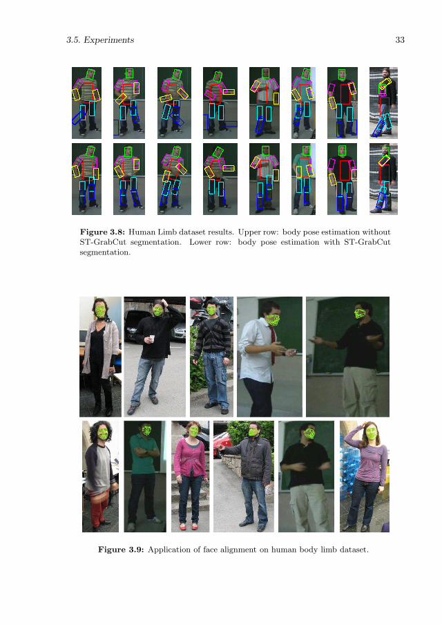
3.5. Experiments 33
Figure 3.8: Human Limb dataset results. Upper row: body pose estimation withoutST-GrabCut segmentation. Lower row: body pose estimation with ST-GrabCutsegmentation.
Figure 3.9: Application of face alignment on human body limb dataset.
34 BINARY HUMAN SEGMENTATION
3.6 Discussion
We presented an evolution of the semi-automatic GrabCut algorithm for dealing with theproblem of human segmentation in image sequences. The new fully-automatic ST-GrabCutalgorithm uses a HOG-based person detector, face detection, and skin color model to initializeGrabCut seeds. Spatial coherence is introduced via Mean Shift clustering, and temporalcoherence is considered based on the historical of color-related Gaussian Mixture Modelsand the trimap initialization for the next frame. The segmentation procedure is combinedwith Shape and Active Appearance models to perform face alignment, and a CRF model isused for human pose estimation.
This general and fully-automatic human segmentation methodology showed higher per-formance than simple GrabCut, in terms of segmentation accuracy. Moreover, we showedhow the proposed segmentation method yields better results in face and body pose recovery,when using it as a pre-processing step in public image sequences and a novel Human Limbdataset from uncontrolled environments.
One of the limitations of the proposed ST-GrabCut method is that it depends on theinitialization step algorithm, which basically depends on the person and face detectors.Initially, we wait until at least one bounding box is returned by the person detector. Thisis a critical point, since we will trust the first detection and start segmenting with thishypothesis. In contrast, there is no problem if a further detection is missed, since we initializethe mask with the previous detection (temporal extension). Moreover, due to its sequentialapplication, false seed labeling can accumulate segmentation errors along the video sequence.
As future work, it would be interesting to combine human segmentation and human poseestimation methods in a same optimization framework. We have seen how a prior segmen-tation of people appearing in a scene can yield much better results when estimating theirpose, but maybe the reverse approach can be also interesting, i.e. human pose estimationcould help segmentation to obtain better results.

Chapter 4
Multi-label human segmentation
4.1 Introduction
In the previous chapter we presented a methodology for segmenting people from the back-ground in video sequences, based on graph cuts optimization. In this chapter, we present amethodology for obtaining finer-detailed segmentations of the human body, classifying pixelsbelonging to the different body limbs, instead of a simple binary classification (foreground,background).
We present a framework for multi-label object segmentation using depth maps based onRandom Forest and Graph Cuts theory, and apply it to the segmentation of human limbs.First, from a set of random depth features, Random Forest is used to infer a set of label prob-abilities for each data sample. This vector of probabilities is used as unary term in α-β swapGraph cuts algorithm. Moreover, depth values of spatio-temporal neighboring data pointsare used in the pair-wise potential. Results on a new multi-label human depth dataset showhigh performance in terms of segmentation overlapping of the novel methodology comparedto classical approaches.
4.2 Related work
Human motion capture is an essential acquisition technology with many applications incomputer vision. However, detecting humans in images or videos is a challenging problemdue to the high variety of possible configurations of the scenario, such as changes in thepoint of view, illumination conditions, and background complexity. An extensive researchon this topic reveals that there are many recent methodologies addressing this problem [24,30, 31, 78]. Most of these works focus on the extraction and analysis of visual features.For example, the work of Bray et al . [21] presents a method that integrates segmentationand 3D pose estimation of a human body from multiple views. These methods have made abreakthrough in the treatment of human motion capture, achieving high performance despitethe occasional similarities between the foreground and the background in the case of changesin light or viewpoint. In order to treat human pose recovery in uncontrolled scenarios,an early work used range images for object recognition or modeling [76]. This approachachieved a straightforward solution to the problem of intensity and view changes in RGBimages through the representation of 3D structures. The progress and spread of this methodcame slowly since data acquisition devices were expensive and bulky, with cumbersome
35

36 MULTI-LABEL HUMAN SEGMENTATION
communication interfaces when conducting experiments. In late 2010, Microsoft launchedthe Kinect, a cheap multisensor device based on structured light technology, capable ofcapturing visual depth information (RGBD technology, from Red, Green, Blue, and Depth,respectively). The device is so compact and portable that it can easily be installed in anyenvironment to analyze scenarios where humans are present. Before Kinect, in the lastdecade, researchers have also used different methodologies and techniques for constructing3D structures, such as stereoscopic images [32, 95]. However, in this case the problemsof different lighting conditions and calibration still exist. Some of the research has alsofocused on the use of time-of-flight range cameras (TOF) for human parts detection andpose estimation [41, 73, 94], combining depth and RGB data [51].
Following the high popularity of Kinect and its depth capturing abilities, there exists astrong research interest for improving the current methods for human pose and hand ges-ture recognition. While this could be achieved by inter-frame feature tracking and matchingagainst predefined gesture models, there are scenarios where a robust segmentation of thehand and arm regions are needed, e.g. for observing upper limb anomalies or distinguishingbetween finger configurations while performing a gesture. In this sense, depth informationappears quite handy by reducing ambiguities due to illumination, colour, and texture diver-sity. Many researchers have obtained their first results in the field of human motion captureusing this technology. In particular, Shotton et al. [79] presented one of the greatest advancesin the extraction of the human body pose from depth images, an approach that also formsthe core of the Kinect human recognition framework. The method is based on inferring pixellabel probabilities through Random Forest (RF), using mean shift to estimate human joints,and representing the body in skeletal form. Other recent work uses the skeletal model inconjunction with computer vision techniques to detect complex poses in situations wherethere are many interacting actors [62].
Currently, there exists a steady stream of updates and tools that provide robustnessand applicability to the device. In December 2010, OpenNI [6] and PrimeSense [7] releasedtheir own Kinect open source drivers and motion tracking middleware (called NITE [4])for PCs running Windows (7, Vista, and XP), Ubuntu and MacOSX. FAAST (FlexibleAction and Articulated Skeleton Toolkit) is a middleware developed at the University ofSouthern California (USC) Institute for Creative Technologies that aims to facilitate theintegration of full-body control within virtual reality applications and video games whenusing OpenNI-compliant depth sensors and drivers [2, 82]. In June 2011, Microsoft releaseda non-commercial Kinect Software Development Kit (SDK) for Windows that includes Win-dows 7-compatible PC drivers for the Kinect device [3]. Microsoft’s SDK allows developersto build Kinect enabled applications in Microsoft Visual Studio 2010 using C++, C# orVisual Basic. There is also a third set of Kinect drivers for Windows, Mac and Linux PCsby the OpenKinect (libFree- Nect) open source project [5]. Code Laboratories CL NUI Plat-form offers a signed driver and SDK for multiple Kinect devices on Windows XP, Vista, and7 [1]. Finally, last advances in the field have shown outperforming results in 3D human poseestimation from RGB images [50].
4.3 Method overview
We present a framework for multi-label object segmentation using depth maps based onRF and Graph cuts theory (GC) and apply it to the segmentation of human limbs. As wehave seen in previous chapters, the use of GC theory has been applied to the problem ofimage segmentation, obtaining successful results [17, 47, 49]. RF is used to infer a set ofprobabilities for each data sample, each one indicating the probability of a pixel to belong

4.4. Random Forests for body part recognition 37
to a particular label. Then, this vector of probabilities is used as unary term in the α − βswap GC algorithm. Moreover, depth of neighbor data points in space and time are used aspair-wise potentials. As a result, we obtain an accurate segmentation of depth images basedon the defined energy terms. Moreover, as long as we have a priori likelihoods representingtarget appearance, the presented method is generic enough to be applicable in any otherobject segmentation scenario. Our method is evaluated on a 3-D data set designed in ourlab, obtaining higher segmentation accuracy compared to standard segmentation approaches.
The depth-image based approach suggested in [79] interprets the complex pose estimationtask as a classification problem by evaluating the likelihood of each depth pixel to be as-signed a body part label, using the corresponding Probability Distribution Functions (PDF).The pose recognition phase is addressed by re-projecting the pixel classification results andinferring the 3D positions of several skeletal joints using the RF and mean-shift algorithms.The work of [79] shows a number of achievements and improvements over previous work,most notably the growing of a randomized decision forest classifier based on decision treesapplied on simple and computationally efficient depth features.
Our goal is to extend the work of [79] and combine it with a general segmentationmethod based on GC optimization optimization to define a globally optimum segmentation ofobjects in depth images. As a case study, we segment pixels belonging to the following sevenbody parts1: LU/LW/RU/RW for arms, (from Left, Right, Upper and loWer, respectively),LH/RH for hands, and the torso. The pipeline of the segmentation framework is illustratedin Fig. 4.1.
4.4 Random Forests for body part recognition
Considering a priori segmented human body from the background in a training set of depthimages I , the procedure for growing a randomized decision tree λ is formulated over thesame definition of a depth comparison feature as defined in [79]:
ψθ(zi) = zi+ uzi+u
− zi+ vzi+v
, (4.1)
where zi is the depth at pixel i in image I , and θ = (u, v), is a pair of offsets u and v, thenormalization of which ensures depth invariance. Thus, each θ determines two new pixelsrelative to zi, the depth difference of which accounts for the value of ψθ(zi). Each treeconsists of split and leaf nodes (the root is also a split node), as depicted in the upper part ofFig. 4.1. The training procedure of a given tree λ over a unique set of ground truth images(avoiding to share images among different trees), runs through the following steps:
1. Define a set Φ of node splitting criteria φ = (θ, τ ) , through the random selection ofθ = (u, v), and τ ∈ R (a set of splitting thresholds for each θ), with both θ and τ lyingwithin some predefined range limits. After training, each split node will be assignedwith its optimal φ value from Φ.
2. Define a set Z of randomly selected pixels zi over the entire set of training images forthe tree, where the number of pixels per image is fixed. Estimate the PDF of Z overthe whole set of labels L (in our case |L| = 7):
PZ(c) =hZ(c)
|Z|, c ∈ L, (4.2)
1Note that the method can be applied to segment any number of labels of any object containedin a depth image.

38 MULTI-LABEL HUMAN SEGMENTATION
Figure 4.1: Pipeline of the presented method, including the input depth informa-tion, Random Forest, Graph-cuts, and the final segmentation result.
where hZ(c) is the histogram of the examples from Z associated with the label c ∈ L.Each example from Z enters the root node, thus ensuring optimal training of the treeλ.
3. At the currently being processed node (starting from the root), split the (sub)set Z,entering this node into two subsets ZL and ZR obeying Eq. (4.1):
ZL(φ) = i | ψθ(zi) < τ, φ = (θ, τ ),ZR(φ) = Z \ ZL,
(4.3)
and estimate the PDF of ZL, PZL(c), as defined in Eq. (4.2). Compute the PDF of
ZR, which may be speeded up by the following formulae:
PZR(c) =
|Z|
|ZR(φ)|PZ(c)−
|ZL(φ)|
|ZR(φ)|PZL
(c), c ∈ L. (4.4)
4. Estimate the best splitting criterion φ∗ for the current node, so that the informationgain GZ(φ
∗) of partitioning set Z entering the node into left and right subsets to be

4.4. Random Forests for body part recognition 39
maximum:
GZ(φ) = H(Z)−|ZL(φ)|
|Z|H(ZL(φ))−
|ZR(φ)|
|Z|H(ZR(φ)), φ = (θ, τ ) ∈ Φ, (4.5)
whereH(Z) = −∑c∈L
PZ(c) ln(PZ(c)) represents Shannon’s entropy for the input (sub)set
Z and its splits (ZL and ZR) over the set of labels L. It is more or less obvious thatGZ(φ) > 0, φ ∈ Φ, but it is difficult to make a more analytical statement for thebehaviour of GZ(φ). That is why we also use the full search approach to evaluate φ∗:
φ∗ = argmaxφ∈Φ
GZ(φ). (4.6)
5. Recursively repeat step 3 and 4 over ZL (φ∗) and ZR (φ∗) for the left and right nodechildren respectively until some preset stop conditions are met: the tree reaches max-imum depth; the information gain or the number of pixels in the node falls belowa minimum. The node where the stop condition occurred is treated as a leaf node,where, instead of φ∗, the respective PDF for the subset Z reaching the node is stored(see Eq. (4.2)).
Once trained, such a randomized tree serves as a pixel-wise classifier for a test depth image.Each image pixel zi is tested through the tree, starting from the root and ending at a leafnode, taking a path that only depends on the inequality ψθ(zi) < τ , using the splittingcriterion φ = (θ, τ ) stored at the tree nodes. Finally, the pixel is tested against the PDFkept at the reached leaf node. Because of the random factor when growing the tree, differenttrees have different predictions for the pixels of the same image. It cannot be stated thatone tree is a better single classifier than another one since each tree is fitted to its trainingset. But an ensemble of trees, which form a random forest Λ, is expected to increase thepredictive power of the classifier. Therefore, the inferred pixel probability distribution withinthe forest is estimated by averaging the PDFs over all trees in the forest as follows:
P (c | zi) =1
|Λ|
∑
λ∈Λ
Pλ (c | zi) , c ∈ L, (4.7)
where Pλ (c | zi) is the PDF stored at the leaf, reached by the pixel zi and traced throughthe tree λ ∈ Λ. Assuming that trees in the forest Λ are fairly balanced, the time complexityof classifying an image is O(|Λ| ·N · dmax), where N is the total number of pixels from theimage I and dmax is the averaged maximum depth level over the trees of Λ.
The randomized tree growing process suggested by Shotton et al. [79] involves two levelsof randomness: in choosing the training images and in the random definition of the nodesplitting criteria. This ensures minimum correlation among the trees in the forest. UnlikeBreiman’s classic Random Forest algorithm [81], which chooses the best split candidate(criterion) among a small subset of all possible candidates, the presented split candidateselection procedure greedily explores all possible choices in order to guarantee the mostefficient split at the current node. The after-effects are two: the most informative featuresare filtered down and pushed onto the tree; similar pixels have better chances of fallingwithin the same descendant nodes. The estimated time complexity of building a randomizeddecision tree under the above conditions is O(|Φ| · |Z| · dmax).
We apply the RF methodology of [79], as described above, in the following two use cases:for rough detection of the main body parts, and for detailed segmentation of the fingers ofthe hands (to eventually be applied for sign-cued language recognition problems).

40 MULTI-LABEL HUMAN SEGMENTATION
4.5 Multi-limb human segmentation
In this section, we formulate an energy minimization problem for multi-limb segmentation ofthe human body, based on the GC optimization framework. More specifically, we rely on theoutput from the previous RF approach applied on depth images, and optimize it introducingspatio-temporal consistency via the GC graph topology.
Given the set of frames I = I1, ..., It, ...; IM, of a video sequence, and z = (z1, ..., zi, ..., zN·M )the array of pixels of I, N as the set of unordered pairs i, j of neighboring pixels inspace and time, under a defined neighborhood system –typically 6- or 26-connectivity–, andf = (f1, ..., fi, ..., fN·M ) a vector whose components fi specify the labels assigned to pix-els in video sequence I. We define the following energy function E whose minimum valuecorresponds to the optimal solution to our problem:
E(f , z) =
N·M∑
i=1
Di(fi, zi) +∑
i,j∈N
Vi,j(fi, fj , zi, zj). (4.8)
The unary potential is defined as the negative logarithm of the likelihood of each pixelto be classified as a certain human limb, computed by the RF approach (Equation 4.7):
Di(fi, zi) = − log(P (fi|zi)). (4.9)
The pair-wise potential encodes contextual information by introducing penalties to eachpair of neighboring pixels as follows:
Vi,j(fi, fj , zi, zj) = Γ · Ω(fi, fj) ·1
dist(i, j)e−β‖zi−zj‖
2
, (4.10)
where β =(2〈(zi − zj)
2〉)−1
, dist(i, j) computes the Euclidean distance between the cartesiancoordinates of pixels zi and zj and Γ ∈ R
+ is a weight that specifies the relative importance ofthe boundary term against the unary term. Finally, the function Ω(fi, fj) is a generalizationof the Potts model to the multi-label case, introducing prior costs between each possible pairof neighboring labels.
We defined two different Ω(fi, fj) functions in order to introduce some prior costs betweendifferent labels. On one hand, we considered the trivial case where all different labels havethe same cost, generalizing the Potts model to the multi-label case:
Ω1(fi, fj) =
0 for fi = fj1 for fi 6= fj .
(4.11)
On the other hand, we introduced some spatial coherence between the different labels,taking into account the kinematic constraints of the human body limbs:
Ω2(fi, fj) =
0 for fi = fj10 for fi = LU, fj = RU
fi = LH, fj = RH5 for fi = LW, fj = RH
fi = RW, fj = LH1 otherwise .
(4.12)
With this definition of the inter-label costs, we complicate the optimization algorithm tofind a segmentation in which there exists a frontier between the right and left upper-arms,right and left hands, or in the lower measure, between left hand and right lower-arm, and

4.6. Experiments 41
Figure 4.2: Graph topology introducing temporal coherence.
vice-versa. Therefore, we are assuming that poses in which the two hands are touching arenot probable2.
In order to build the graph for the energy function optimization, we adopt a 3-D gridtopology that introduces spatial and temporal connections between pixels of the video se-quence. We define a 10-connectivity pattern for the pixel neighborhood system (8 spatialand 2 temporal neighbors), shown in Fig. 4.2. From a practical point of view, and con-sidering that computer memory resources are limited, we adopt a sliding-window approach.More specifically, we define a fixed size volume window of M frames i.e. M frames will besimultaneously segmented in a single execution of the optimization algorithm.
The sliding-window approach starts segmenting the first M frames, and covers all thevideo sequence volume, with a one-frame stride. This means that all the frames except thefirst and the last one are segmented at least twice and M times at most. In order to selectthe final hypothesis for each frame, we use the energy value resulting from the minimizationalgorithm at each execution. Therefore, the execution with the lowest energy value is theone we trust as the best hypothesis.
As we reviewed in Chapter 2, multi-label graph cuts optimization can be performed viatwo different algorithms; depending on the choice of the pair-wise potential V , we could useα-expansion (in case V is a metric), or α-β swap (if V is a semi-metric). In our case, wehave that Ω1(fi, fj) satisfies the conditions to be a metric, so α-expansion can be used inorder to find the solution. In contrast, Ω2(fi, fj) does not meet all the necessary conditionsto become a metric (it is a semi-metric instead), so α-β swap must be used in this case.
4.6 Experiments
We first describe the considered data for the experiments, the different methods, parametersand validation protocol of the evaluation. Next we present results for pixel classification
2This label coherence cost should be estimated for each particular problem domain. In ourparticular dataset of poses, the values of 1, 5, and 10 were experimentally computed.

42 MULTI-LABEL HUMAN SEGMENTATION
Figure 4.3: Interface for semi-automatic ground-truth generation.
using Random Forest, and the results obtained when applying multi-label segmentation.
4.6.1 Data
For the purposes of gathering ground truth data, we defined a new dataset of several videosequences where the actors are performing different gestures with their hands in front of aKinect camera – only the upper body is considered. See Fig. 4.4 for some pose samples. Eachframe is composed by one 24 bit RGB image of size 640x480 pixels, one 12 bit depth bufferof the same dimension, and a skeletal graph describing relevant joints of the upper humanbody. In order to label every pixel we created a special editing tool to facilitate labellingin a semi-supervised manner. Each frame is accompanied with label buffer of the samedimension as the captured images. The label buffer is automatically initialized through arough label estimation algorithm. The pixels bounded by the cylinders between the enclosingjoints of the shoulder to elbow are labelled as upper arm (LU/RU). By analogy the pixelsinside the cylinder between the elbow and the joint of the hand are labelled as lower arm(LW,RW). The palm is labelled by the pixels bounded by a sphere centered in the joint ofthe hand (LH,RH). The RGB, depth, and skeletal data are directly obtained via the OpenNIlibrary [6]. Finally each frame is manually edited to correct the roughly estimated labelsby the initialization algorithm. The whole ground truth used in our experiments is createdfrom capturing 2 actors in 3 sessions gathering 500 frames in total (15 fps). It should benoted that after the manual editing there still exist around 1% of false positive labels dueto editor mistakes. An example of the developed interface for semi-automatic ground-truthgeneration is shown in Figure 4.3. See Appendix A for more information on how to obtainthe dataset.
We also made an extra experiment for finger segmentation defining 6 labels per hand -one label for each finger and one for the palm. For gathering ground truth data from thefingers, we applied another initialization algorithm using coloured gloves, with each fingerbeing painted with a different colour. Finally manual editing is still necessary due to thehigh level of false positive errors. 63 frames are generated and used in the experiment.

4.6. Experiments 43
4.6.2 Methods and validation
In the first place, we analyze the results obtained directly using the probabilities returnedby the RF approach. The RF algorithm used for the experiments computation has beenimplemented following the description of Shotton et al. [79]. In the same way, inspired by thereported test parameters and accuracy results in [79], our experiments rest on the followingsetup: we perform a 5-fold cross-validation over the available 500 frames by training randomforest of Λ = 3 trees, therefore 130 unique training images per tree, with 1, 000 uniformlydistributed pixels per image. We limit the maximum depth level dmax for all trees to 20, anduse 100 candidate offset pairs θ, and 20 thresholds τ per θ to build the splitting criteria Φ.The remaining 100 images form the test set. Carrying a randomized test trial, we analyzethe effect of the choice of test parameters on the classification accuracy and compare theresults with another set of features: a mixture of the original depth features ψθ(zi) fromEq. (4.1) and new features ψθ(zi) based on the depth gradient:
ψθ (zi) = ∡
(
(zi+ u
zi+u
),
(zi+ u
zi+v
)), (4.13)
where (zi) is the gradient of depth at pixel zi. In fact, the new feature ψθ(zi) representsthe angle between the two gradient vectors at offsets u and v from i.
In second place, we compare our proposed segmentation approach with the state-of-the-art Random Walks (RWalks) image segmentation algorithm [44], both applied to theprobability maps returned by the execution of the RF method. Since RWalks is designed tosegment still images, no temporal coherence is taken into account in this approach. Further-more, besides the probability maps, RWalks also receives some user-designed seeds, since itis semi-automatic. However, in order to perform a fair comparison between this method andour proposal, which is fully-automatic, we need to automatize the seed-selection process.For this task, we select the seeds for each label as the pixels with greatest probability value.When applying GC, the Γ parameter was set to 50 for all the performed experiments, andthe size of the sliding window is set to M = 5.
In order to achieve a more appropriate comparison of the results, we perform an addi-tional GC experiment consisting on removing the temporal coherence, i.e. segmenting eachframe of the sequence independently, using a 2-D lattice graph topology with 8-connectivity.Furthermore, in this second experiment we also compare the performance of prior cost func-tions Ω1 and Ω2, as well as the use of different pixel information for the computation of thepair-wise potential. In addition to depth information, we also test including RGB informa-tion to the pair-wise potential by normalizing depth information in the range [0...255] andconcatenating it with RGB values, resulting in a 4-dimensional RGBD vector for each pixel.
Finally, we also apply the Friedman test [33] in order to look for statistical significanceof the performed experiments.
4.6.3 Random forest pixel-wise classification results
Table 4.1 shows the estimated average classification accuracy for each of the considered labels.The most likely label predicted for a pixel is chosen to be the one that corresponds to themaximum of the inferred RF probabilities for that pixel. Without claiming exhaustivenessof our experiments, the results from Table 4.1 allow us to make the following analysis: Theupper limit Omax for the module of u and v offsets has the greatest impact on the accuracyresults at the hands regions, which have the smallest area in our body part definition.Doubling Omax leads to an increase in the accuracy of about 20% for the hands and about6% for the other body parts. In other words, higher Omax values increase the featurediversity and the global ability to represent spatial detail. The number of candidate offset

44 MULTI-LABEL HUMAN SEGMENTATION
Table 4.1: Average per class accuracy in % calculated over the test samples in a5-fold cross validation. ψθ represents features of the depth comparison type fromEq. (4.1), while ψθ - the gradient comparison feature from Eq. (4.13). Omax is theupper limit of the u and v offsets, and dmax stands for the maximal depth level ofthe decision trees.
Setup Performance
ψθ ψθ Omax dmax Torso LU LW LH RU RW RH Avg.
100 0 30 20 92.90 73.29 71.42 57.75 74.25 76.26 59.38 72.1880 0 60 20 94.22 79.08 76.46 74.19 81.24 83.26 79.05 81.0760 0 60 20 94.09 78.86 75.86 73.49 79.43 82.60 78.08 80.34100 0 60 20 94.17 79.83 77.69 77.10 81.04 82.65 80.17 81.81100 0 60 15 94.06 79.81 78.69 76.59 81.18 83.10 80.23 81.95
100 0 60 10 91.83 81.47 78.98 72.30 83.00 83.74 76.85 81.1760 20 60 20 94.04 77.73 74.93 71.97 77.62 81.22 76.64 79.17
pairs θ would not have such a tremendous impact on the accuracy as the Omax parameter,although a higher number of θ candidates would help in identifying the most discriminativefeatures. A decrease of the number of candidates from 100 to 80 features drops the handsaccuracy by 1− 3%.
We also tested the impact of dmax, the depth level limit of the decision trees. Trimmingthe trees to level 15 has a very little impact, showing an improvement of 0.1% on the averageaccuracy. The latter may be weakly attributed to better classification at the lower armregions. Trimming to depth level 10 shows a 4% decrease in the accuracy at the hands. Ouranalysis indicates that we may be witnessing slight overfitting at tree depth level of 20 dueto the small amount of training images. Our final test includes comparison over combinationof both features ψθ and ψθ of Eq. (4.1) and Eq. (4.13). Since the depth data provided byKinect is noisy, we apply a Gaussian smoothing filter before calculating the image gradientsand the ψθ features. We chose the gradient feature since it complements the relations ofdepth features with information about the orientation of local surfaces. However, in our testwe did not find significant improvement in the performance results of the RF approach.
In order to show the generalization capability of the proposed approach, we carried outan extra case study, stressing on the segmentation of the finger regions. For this test we onlyconsidered a manual annotated set of 63 depth image frames without including temporalcoherence. The results applying the same validation as in the previous case show the bestperformance for the following setup: 1 tree of depth 15, 500 pixels per image, 100 candidateoffset pairs θ, 20 candidate thresholds τ , and Omax = 45. The estimated average per classaccuracy was 58.5%, mostly due to the small number of training images. Fig. 4.5 displays acouple of test images comparing the ground truth and the inferred labels for the fingers andhands. Reviewing the classification results from both use cases, the body parts and fingerregions, we observe that some of the errors appear due to left/right uncertainty. Nevertheless,the results are promising, showing the generalization ability of the presented approach forgeneral multi-class labelling in depth images.
4.6.4 Multi-label segmentation results
The results we obtained when applying GC over the probabilities returned by the RF aredetailed in Table 4.2. We can see how these results improved the labelling obtained by theRF approach, and also the one obtained in the frame-by-frame approach. Moreover, allthe GC approaches shown in Table 4.2 outperform the results obtained using the RWalks
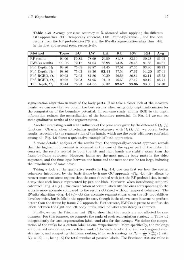
4.6. Experiments 45
Table 4.2: Average per class accuracy in % obtained when applying the differentGC approaches –TC: Temporally coherent, Fbf: Frame-by-Frame– , and the bestresults from the RF probabilities [79] and the RWalks segmentation algorithm [44],in the first and second rows, respectively.
Method Torso LU LW LH RU RW RH Avg.
RF results 94.06 79.81 78.69 76.59 81.18 83.10 80.23 81.95
RWalks results 99.05 72.17 81.04 86.98 73.27 88.48 91.68 84.67
Fbf, Depth, Ω1 98.86 75.05 82.87 91.45 77.57 87.35 93.96 86.73Fbf, Depth, Ω2 98.86 75.03 83.36 92.41 77.54 87.67 94.20 87.01Fbf, RGBD, Ω1 99.02 72.02 81.86 90.29 76.56 86.84 92.14 85.53Fbf, RGBD, Ω2 99.02 72.03 81.95 91.19 76.53 87.12 92.12 85.71TC, Depth, Ω2 98.44 78.93 84.38 88.32 82.57 88.85 93.86 87.91
segmentation algorithm in most of the body parts. If we take a closer look at the measure-ments, we can see that we obtain the best results when using only depth information forthe computation of the boundary potential. In our case study, adding RGB to the depthinformation reduces the generalization of the boundary potential. In Fig. 4.4 we can seesome qualitative results of the segmentations.
Another interesting result is the influence of the prior costs given by the different Ω (fi, fj)functions. Clearly, when introducing spatial coherence with Ω2 (fi, fj), we obtain betterresults, especially in the segmentation of the hands, which are the parts with more confusionamong all. Fig. 4.6 shows a qualitative example of both approaches.
A more detailed analysis of the results from the temporally-coherent approach revealsthat the highest improvement is obtained in the case of the upper part of the limbs. Incontrast, the results related to both the left and right hands are slightly worse than theframe-by-frame approach. However, hands are the most moving body parts in the videosequences, and the time lapse between one frame and the next one can be too large, inducingthe introduction of some noise.
Taking a look at the qualitative results in Fig. 4.4, one can first see how the spatialcoherence introduced by the basic frame-by-frame GC approach –Fig. 4.4 (d)– allows torecover more consistent regions than the ones obtained with just the RF probabilities, in sucha way that each limb is represented by just one blob. Moreover, when introducing temporalcoherence –Fig. 4.4 (e)–, the classification of certain labels like the ones corresponding to thearms is more accurate compared to the results obtained without temporal coherence. TheRWalks algorithm –Fig. 4.4 (c)– obtains accurate segmentations when the RF probabilitieshave low noise, but it fails in the opposite case, though in the shown cases it seems to performbetter than the frame-by-frame GC approach. Furthermore, RWalks is prone to confuse thelabels between the right and left body limbs, since no label consistency is enforced.
Finally, we use the Friedman test [33] to show that the results are not affected by ran-domness. For this purpose, we compute the ranks of each segmentation strategy in Table 4.2independently for each segmentation label –and also for the average. We define the compu-tation of the ranks for a certain label as one “experiment”. More specifically, the rankingsare obtained estimating each relative rank rsc for each label c ∈ L and each segmentationstrategy s, and computing the mean ranking R for each strategy as Rs = 1
NF
∑NFi=1 r
si with
NF = |L|+ 1, being |L| the total number of possible labels. The Friedman statistic value is

46 MULTI-LABEL HUMAN SEGMENTATION
(a) (b) (c) (d) (e)
Figure 4.4: Qualitative results; Ground Truth (a), RF inferred results (b), RWalksresults (c), frame-by-frame GC results (d), and Temporally-coherent GC results (e).

4.7. Discussion 47
then computed as follows:
X2F =
12NF
k(k + 1)
[∑
s
R2s −
k(k + 1)2
4
]. (4.14)
In our case, with k = 7 segmentation strategies to compare, NF = 8 different experi-ments, and ranks R = [5.63, 4.88, 2.5, 3, 2.75, 4.75, 4.5] in the row order of Table 4.2,X2
F =15.48. Since this value is undesirable conservative, Iman and Davenport proposed a correctedstatistic:
FF =(NF − 1)X2
F
NF (k + 1)−X2F
. (4.15)
Applying this correction we obtain FF = 3.38. With seven strategies and eight experi-ments, FF is distributed according to the F distribution with six and 42 degrees of freedom.The critical value of F (6, 42) for 0.05 is 2.23. As the value of FF is higher than 2.23 we canreject the null hypothesis, and thus, looking at the best mean performance in Table 4.2, wecan conclude that the spatio-temporal GC proposal is the best choice from the presentedexperiments.
In the second experiment, labelling pixels from hands –in a frame-by-frame fashion, weachieve an average per class accuracy of 70.9%, which supposes even a greater improvementthan in the case of human limbs. Fig. 4.5 shows some qualitative results of the GC approach,where we can appreciate that regions are more consistent and better defined than in the caseof just using RF probabilities. It is worth mentioning that for this experiment we usedΩ1 (fi, fj) as the cost function between labels, and yet we obtained consistent results.
4.7 Discussion
We proposed a generic framework for object segmentation using depth maps based on Ran-dom Forest and Graph cuts theory in order to benefit from the use of spatial and temporalcoherence, and applied it to the segmentation of human limbs. Random Forest estimatedthe probability of each depth sample point to belong to a set of possible object labels, whileGraph-cuts was used to optimize, both spatially and temporally the RF probabilities. Re-sults on two novel datasets showed higher performance segmenting several body parts indepth images, compared to state-of-the-art approaches.
Among the different parameters of the Random Forest method for pixel-wise classifica-tion, we saw that the upper limit Omax on the module of offsets u and v when computingdepth comparison features ψθ plays an important role in the final performance of the system.When choosing the appropriate value for Omax, the pixel-wise classification mean accuracyincreases in a 10%, yielding a especially higher 20% performance boost in the accuracy ofhand region classification.
When enforcing spatio-temporal consistency on the classification by applying multi-labelGraph cuts optimization on the probabilities computed by Random Forest, we showed thatadding asymmetric costs between different labels via the defined Ω2(fi, fj) function (Eq. 4.12)yields better results, especially in the case of the upper part of the body limbs. While notensuring any approximation factor w.r.t the optimal solution, α-β swap yields better resultswhen using the asymmetric label cost assignments defined by Ω2(fi, fj) than the solutionfound by α-expansion and the multi-label generalization of the Potts model Ω1(fi, fj).
As interesting future research lines, such fine-grained segmentation masks of the humanbody could be used to extract body pose features (especially in the case of the hands), and

48 MULTI-LABEL HUMAN SEGMENTATION
Figure 4.5: Results from RF classification in the case of hands. First row showsthe ground-truth for two examples. Second row shows the RF classification results.Third row shows the final α-expansion GC segmentation results.
(a) (b)
Figure 4.6: Comparison of results without (a) and with (b) spatially-consistentlabels.

4.7. Discussion 49
apply them to recognize gestures, for human-computer interaction and smart environmentapplications.

50 MULTI-LABEL HUMAN SEGMENTATION

Part II
Human Pose Estimation
51


Symbol notation in Part II
Table 4.3: Symbols and conventions for chapters 5- 6
L = l1, ...lM Set of M parts of an articulated object, li(xi, yi) Part positionθi Part rotationsi Part scale
G =< V, E > CRF graph composed of nodes V and edges Evi node in V, representing part li.eij edge in E connecting nodes i and jE Energy function for the PS modelEu
i Unary potential for node iEu
i,j Pair-wise potential for edge between nodes i and jI Image
In, Ln Training set, n = 1, ..., N , composed by N pairs of images andpart configurations
β = (βu, βp) Parameters of the PS model
ti Type index of part liT Number of types for each part in the DPM model
S(I, L,β) Score function of the DPM modelSui Score unary term for part li
Spi,j Score pair-wise term for the connection between parts li and ljSb Score bias term
β = (βu, βp, βb) Parameters of the DPM modelφ(I, xi, yi) Feature extraction functionψ(li, lj) Vector of position differences between parts li and ljmi(lj) Message from part i to its parent j
scorei(li) Local score at part iξn Slack variable
P Number of poselets in the mid-level part representationP Set of P poselet detectorsP ′ Initial random number of poselet candidatesBp′ Bounding box with position (xp′ , yp′), width wip′ , height hep′
and scale sp′τproc Threshold on the Procrustes alignment costωp′ Detector for poselet proposal p′
(xgtk , y
gtk ) Ground-truth annotations for the body joint k
53

54
(µkp′ ,Σ
kp′) Gaussian distribution on the spatial coordinates of keypoint k
among the training samples for poselet detector proposal p′
A Binary matrix of poselet activations in the validation setxp′ Binary variable of the Integer Program for poselet selection
P Set of poselet detectionsCP
i Set of contextual feature vectors between body part li and PG Number of detections taken from each poselet p ∈ P
R(C) Rescoring function given the set of contextual feature vectors CQθ Weak set classifierΘ Number of weak set classifiersqθ Weak item classifiers (decision trees)αθ Weight of weak set classifier Qθ
kc Relevance of item c ∈ CF Number of leaves in decision trees qθ
U1, ..., UF F Partitions of the feature space given by leaves in qθαf Weights of leaf nodes in qθλ Regularization parameter
L(·) Loss function
Hf Total sum of relevance of items falling in partition Uf
yBiLabel of bounding box Bi from a detection of part li
O(Bi, Bj) Overlapping between bounding boxes Bi and Bj
βtii Weight of the rescoring function in the DPM score function
Eu,boost Local appearance unary potentialEu,poselets Poselet evidence unary potential
βuw Weight of the rescoring function in the PS energy function

Chapter 5
Detecting people: Part-based object
detection
5.1 Introduction
Detecting rigid objects in images has been commonly formulated as a binary classificationproblem, where input subregions of a given image are classified as positive or negative,whether a specific object is present in that subregion or not, respectively. Some well-knownexamples of such methodologies are face detection [88], or pedestrian detection [30] (seeFig. 5.1). Given that the appearance variability of these objects is relatively low, the classifierlearns subregions of a specific aspect ratio. In contrast, articulated objects have a muchhigher variability of their shape and appearance, hence more sophisticated models are neededin order to capture these object deformations.
In particular, part-based models have proven high performance rates for object detection.The main idea behind part-based models is the decomposition of an object into a set of parts
Linear SVM
Figure 5.1: Pedestrian detection as a classic sliding-window approach for objectdetection. HOG features extracted from candidate bounding boxes in the image aretested against a Linear SVM trained on images of people, which predicts a positive(green) or negative (red) answer for each candidate window.
55

56 DETECTING PEOPLE: PART-BASED OBJECT DETECTION
connected to each other following a class-specific topology. The motivation for this is that,while the global appearance of an articulated object may vary considerably when sufferingdifferent deformations, the appearance of some of its parts may not be significantly altered.Therefore, detecting an articulated object is reduced to detecting its parts (considered asnew object classes) and applying a known relational model that fosters spatially-consistentpart configurations.
In this chapter we briefly introduce two methodologies for part-based object detection,successfully used to tackle the problem of human pose estimation: pictorial structures (PS)and deformable part models (DPM).
5.2 Pictorial structures
As mentioned in the introduction, articulated object detection is usually tackled by learninga model formed by different connected parts. Pictorial structures proposed by Felzenswalband Huttenlocher [38] follow this philosophy by modeling an object as a collection of partsarranged in a deformable configuration. More specifically, parts are defined as local ap-pearance templates, while spatial connections between parts can be considered as flexible“springs” (see Fig, 5.2(a)).
(a) (b)
Figure 5.2: (a) Sample pictorial structure for human pose estimation; blue rect-angles depict the different parts of the model (corresponding to parts of the humanbody) and yellow springs show the flexible connections between parts. (b) The cor-responding CRF for the pictorial structure model in (a); blue nodes represent theparts of the model and yellow edges codify the spring-like connections.
Let L = l1, ..., li, ...lM be the set of parts of an object, where each part li = (xi, yi, ri, si)is parametrized by its position xi, yi, absolute rotation ri and scale si. Given a graphG =< V, E >, a pictorial structure model is then formulated as a Conditional Random Field(CRF) in which parts li are indexed by nodes vi ∈ V in the graph G, and the set of edgesei,j ∈ E represent the “spring”-like connectivity pattern between nodes (see Fig. 5.2(b)).

5.2. Pictorial structures 57
Similarly to graph cuts optimization reviewed in chapter 2, an energy function associatedto such CRF can then be defined as follows:
E(I, L,β) =M∑
i=1
Eui (I, li, β
ui ) +
∑
(i,j)∈E
Epi,j(li, lj , β
pi,j), (5.1)
where I is an image, Eu and Ep are the unary and pair-wise potentials and βu, βp theirrespective sets of model parameters.
In this case, the unary potential Eui can be considered as a mismatch function for plac-
ing part i in the image under the configuration specified by li, based on appearance cues.Hence, βu
i parameters could be thought of as a classifier for detecting part i and recover itsconfiguration li, e.g . a Linear SVM classifier on HOG features, like in the pedestrian detec-tion example. On the other hand, the pair-wise potential Ep
i,j can be defined as a functionmeasuring the degree of deformation of the “spring” connecting parts i and j under config-urations li and lj , respectively. In this case, parameters βp
i,j are the responsible for learningthe flexibility of the “springs” connecting different parts. Then, given an image at test time,the goal is to find the part configutation L that minimizes the defined energy function:
L∗ = argminLE(I,L,β). (5.2)
5.2.1 Inference
In order to efficiently find the best configuration L∗ of the pictorial structure model, thegraph G defining the topology of the corresponding CRF must not contain any cycles, hencethe topology must be a tree. Then, belief propagation algorithms like sum-product message-passing can be used for efficient exact inference and find L∗.
Given this restriction on the topology for G, the majority of works that use pictorialstructures, define their models following a tree structure. More specifically, works on humanpose estimation like [10, 71] use models like the one shown in Fig. 5.2.
Nevertheless, some other works based on pictorial structures introduce cycles in G, anduse loopy belief propagation for inference. However, this algorithm only allows for approxi-mate inference, so the optimum solution L∗ can not be found efficiently in this case.
5.2.2 Learning
Learning a pictorial structure can be then understood as estimating the parameters β =(βu, βp) of the model. While there are no strict guidelines for parameter estimation, Felzenswalband Huttenlocher [38] proposed Maximum Likelihood Estimation (MLE) for that matter:
β∗ = argmax
β
N∏
k=1
P (Ik | Lk,β)N∏
k=1
P (Lk | β), (5.3)
given a training set In, Ln, n = 1, ..., N composed of N images and their correspondinglabels.
An important fact is that this learning can be done separately for parameters of theunary and pair-wise potentials, βu and βp, respectively. As an example of this, Andriluka etal . [10] learn the unary potential parameters βu
i discriminatively, using Adaboost over shapecontext features extracted from images, and pair-wise parameters βp are learnt as Gaussiandistributions via MLE.

58 DETECTING PEOPLE: PART-BASED OBJECT DETECTION
5.3 Deformable Part Models
Following the same idea of pictorial structures, deformable part models [37, 96] also decom-pose an object into a set of different parts, connected to each other following the topologyspecified by means of a graph G =< V, E >. However, the hypothesis that parts share theappearance among different instances of the object under different deformations, is discarded.
One of the main problems when detecting an articulated object is that some of its partscan be eventually self-occluded by other ones, under certain deformations. Not only that,but slight changes in the viewpoint can result in dramatically different appearances. Weillustrate this in Fig. 5.3, considering the human body as an articulated object, as in themodel shown in Fig 5.2. While some viewpoints and poses of the human body may yield aclear view of most of its parts (see the arms in Fig. 5.3(a)), some other poses may produceself-occlusions of some parts (the arms in Fig. 5.3(b) are occluded by the legs), or evensome parts can appear considerably foreshortened, due to the viewpoint (see upper legs inFig. 5.3(c)).
(a) (b) (c)
Figure 5.3: Different poses of the human body.
In order to deal with these changes in appearance of the parts in the articulated model,the concept of mixtures of parts is introduced. Not only an object is decomposed into a set ofdifferent parts, but each part is defined as a mixture composed of different types of parts. Wefollow the same notation from the previous section and denote by L the configuration of partsin the model. However, in this case each part in the model li = (xi, yi, ti) is parametrizedjust by a position in the image and a type index ti ∈ 1, ..., T, where each part has Tpossible types of parts.
A score function equivalent to the energy funcion in Eq. 5.1 is defined then as:
S(I, L,β) = Sb(L, βb) +
M∑
i=1
Sui (I, li, β
ui ) +
∑
(i,j)∈E
Spi,j(li, lj , β
pi,j), (5.4)
Sb(L, βb) =M∑
i=1
βb,tii +
∑
(i,j)∈E
βb,ti,tji,j , (5.5)
where Sb(L, βb) computes a bias that favors particular assignments for specific parts and
types (parameters βb,tii ), and their co-occurrences (parameters β
b,ti,tji,j ).

5.3. Deformable Part Models 59
The unary term Sui computes the score of considering configuration li, i.e. for placing
part type ti at position (xi, yi) in the image, for part i in the model. More specifically, theunary term is defined as
Sui (I, li, β
ui ) = βti
i · φ(I, xi, yi), (5.6)
where φ(I, xi, yi) represents a feature vector extracted from position (xi, yi) in image I , andβtii are learnt weights on the features (as in the Linear SVM example shown in Fig. 5.1).
The pair-wise term Spi,j computes the agreement between configurations of contiguous
parts i, j in the model:Spi,j(li, lj , β
pi,j) = β
ti,tji,j ψ(li, lj), (5.7)
where ψ(li, lj) = [dx, dx2, dy, dy2], computes first and second order differences dx = xi − xj
and dy = yi − yj among locations (xi, yi) and (xj , yj), and βti,tji,j encode the flexibility of
“springs” connecting parts i, j, tailored to their corresponding types ti, tj .Given this score function, then the problem of detecting an articulated object is defined
as finding the best configuration L∗ with maximum score:
L∗ = argmaxL
S(I, L,β). (5.8)
5.3.1 Inference
As we just explained above, inference corresponds to maximizing the score function S(I, L,β)over L. Again, similarly to pictorial structures, exact inference can be efficiently performedwhen the structure of G is acyclic, i.e. G is a tree, via message passing. The followingmessages from part i to its parent j are computed:
mi(lj) = maxti
βb,ti,tji,j + max
(xi,yi)score(li) + β
ti,tji,j · ψ(li, lj), (5.9)
scorei(li) = βb,tii + βti
i · φ(I, xi, yi) +∑
k∈kids(i)
mk(li). (5.10)
Starting from the leaf nodes to the root, Eq. 5.9 computes for all possible configurations ljfor part j the best scoring location and type of its child part i, and Eq. 5.10 computes thelocal score of part i, collecting messages from its children.
5.3.2 Learning
Since Eq. 5.10 is linear in β, we could write S(I,L,β) = β · Φ(I, L). In order to learnthe parameters β = (βb, βu, βp) of the model, a discriminative approach is considered,similar to a structural SVM. Given a set of labeled positive examples In, Ln, the followingoptimization problem is formulated:
arg minβ,ξn≥0
12β · β + C
N∑n=1
ξn (5.11)
s.t.∀n ∈ pos β · Φ(In, Ln) ≥ 1− ξn (5.12)
∀n ∈ neg β · Φ(In, Ln) ≤ −1 + ξn.
Basically, the constraints of this optimization problem state that positive examples shouldscore more than 1, and negative examples should score less than −1. Violations of theseconstraints are penalized by slack variables ξn. In order to solve this quadratic program,stochastic gradient descent can be used, like in [37].

60 DETECTING PEOPLE: PART-BASED OBJECT DETECTION

Chapter 6
Contextual Rescoring for Human
Pose Estimation
6.1 Introduction
In this chapter we propose a contextual rescoring method for predicting the position ofbody parts in a human pose estimation framework. A set of poselets is incorporated in themodel, and their detections are used to extract spatial and score-related features relativeto other body part hypotheses. A method is proposed for the automatic discovery of acompact subset of poselets that covers the different poses in a set of validation images whilemaximizing precision. A rescoring mechanism is defined as a set-based boosting classifierthat computes a new score for each body joint detection, given its relationship to detectionsof other body joints and mid-level parts in the image. In order to show its adaptability toother methods, we incorporate the proposed rescoring method in two state-of-the-art humanpose estimation frameworks, one of them based in deformable part models [37], and anotherone based on pictorial structures [69]. Experiments on two benchmarks show comparableresults to Pishchulin et al. [69] while reducing the size of the mid-level representation by anorder of magnitude, reducing the execution time by 68% accordingly.
6.2 Related work
In the context of human pose estimation, pictorial structure models have been widely used.Since the search space of such highly-articulated models can be very large, some worksproposed methodologies for reducing it. Ramanan [71] proposed an iterative inference processfor the pictorial structure model. An edge-based appearance model of the body parts is firstlyapplied, giving a rough estimate of their location. Using this rough estimate, a color modelof the foreground and the background is learnt, which helps in reducing the search spaceof the inference. A further extension of this idea was proposed by Ferrari et al . [40]; theydirectly segment the human body from the background of the scene, eliminating the need ofa two-step inference. In contrast, Andriluka et al . [10] proposed to use stronger body partdetectors based on dense shape context features, outperforming previous works.
Since the number of possible poses a person can adopt is huge, usually a simple pictorialstructure model is not able to model all this variability in the data. In order to overcomethis, some works increase the flexibility of pictorial structure models by adding pose prior
61

62 CONTEXTUAL RESCORING FOR HUMAN POSE ESTIMATION
information in the model. For example, Sapp et al . [77] adjust the parameters of the pictorialstructure model (particularly the ones regarding the pairwise potential) depending on imageevidence. Similarly, Johnson and Everingham [52] partition the space of human poses intodifferent clusters and learn specific pose priors and appearance models. In a further extensionof their work [53], they replace a single pictorial structure model by a mixture model, suchthat each component of the model is specialized to a particular region of the pose space.Additionally, they present a new dataset of 10, 000 images that they use as additional trainingdata. Yang and Ramanan [96] followed the same trend and proposed a “flexible mixture ofparts” model. Moreover, they proposed a new formulation of the problem; they modelthe body joints instead of the body parts, thus simplifying the formulation and reducing thecomplexity of inference. Specifically, the body joints are modeled as a mixture of small HOGfilters [30] capturing a small neighborhood around them. While simplifying the inferenceand attaining better results than previous works, the performance of their method is stillcompromised by the use of a tree-structured model.
In contrast, some works have proposed to work with loopy graphs. Tian and Sclaroff [85]augmented the tree model by adding a small set of edges, and presented an efficient infer-ence algorithm for their model. In the experimental section, they show how their methodovercomes the so-called “double-counting” phenomena that tree-structures tipically sufferfrom. [83] proposed a branch-and-bound inference algorithm, allowing to compute exactinference on loopy graph models efficiently. [35] proposed a multi-layer pictorial structuremodel, incorporating body part evidence at different scales; from full body to local parts.In their proposed model, each layer is tree-structured by itself, but edges between adjacentlayers make the whole model a loopy graph. However, this graph can be easily decomposedinto tree-structured subproblems (which are amenable to exact inference), and they showhow inference can be performed via dual-decomposition. Finally, [92] also proposed a hi-erarchical approach. They presented a manually-defined hierarchical decomposition of thehuman body; they introduced poselets ([15, 16]) as new parts in the model, adding also thecorresponding set of higher-order edges with the existing basic parts. Since this extensionresults in a loopy-graph model, the method can only perform approximate inference.
Some recent works propose hierarchical tree models that are able to model high-orderpart dependencies by recursively dividing the human body into different mid-level parts, inaddition to the set of basic body parts. Tian et al . [86] present a hierarchical model whereleaf nodes correspond to body parts, and intermediate latent nodes cover different subsets ofnearby body parts. Similarly, [92] and [90] also included mid-level poselet-based body partsin their pictorial structure model, but they propose an algorithm for discovering the bestpossible tree topology that connects all the parts. In contrast, [68] introduced higher-orderpart dependencies in their pictorial structure model by conditioning the unary and pairwiseterms on poselet evidence. At training time, they cluster the relative distance between aparticular part and the torso, and model this offset as a Gaussian distribution for eachcluster. At test time, they solve a classification problem in which poselet responses are usedto predict the correct cluster and recover the corresponding Gaussian distribution. Thisadditional information about the location of that particular part is then incorporated in thepictorial structure model as an extra unary potential. They proceed analogously to predictpart orientations and to learn the pairwise terms of the model. In a further extension oftheir work, [69] achieve a higher performance by incorporating additional parts that modelbody joints in their pictorial structure, following the idea of flexible spatial models from [96].
A bridge between human pose estimation and object detection was proposed by Yaoand Fei-Fei [97]. They model mutual contextual information between poses and objects fora certain set of human-object interaction activities, like “tennis serve” or “croquet shot.”The results indiciate that pose estimation can help object detection and vice versa. An-

6.3. Method overview 63
Basic part l1
detections
Mid-level part detections
Part l1
context.
features
Part l1
rescoring
PS Model
inference
Pose estimateInput image
Part lM
rescoring
[…]
…
Basic part lM
detections
Part lM
context.
features
[…]
Figure 6.1: Proposed pipeline for human pose estimation. Given an input image, aset of basic and mid-level part detections is obtained. For each basic part detectionli, a contextual representation is computed based on relations with respect to theset of mid-level part detections. Using these contextual representations, basic partdetections are rescored using a classifier for that particular basic part class. Theoriginal and rescored detections for all basic parts are then used in inference on apictorial structure (PS) model to obtain the final pose estimate.
other work on exploiting contextual information between objects was proposed by Cinbisand Sclaroff [25]; they present an approach for rescoring detections of different objects, in-troducing the notion of sets of contextual relations between object detections in an image.Each detection from a certain object class is represented by its context, defined as a set ofdetections from every other object detector. Then, a feature vector is extracted from eachcontextual detection, encoding spatial relations, relative scores and class-related relations. Ageneralization of the well-known Adaboost algorithm, called SetBoost, is used for rescoringan object detection given its set-based context representation.
6.3 Method overview
An overview of the proposed pipeline for human pose estimation is presented in Fig. 6.1.Following the notation used in Chapter 5, we denote by L = l1, ..., lM the set ofM parts inthe model. We propose a method for obtaining robust part detections li in pictorial-structure-based human pose estimation frameworks, motivated by the aforementioned limitations ofbasic, low-level part detectors that are commonly used in pictorial structure models, e.g .HOG patches centered at body joints ([96]). We define and learn an additional set of mid-level body part detectors that improve the localization of the basic ones. Mid-level and basicpart detectors are applied in order to extract a set of pairwise contextual features betweeneach pair of basic and mid-level part hypotheses (see Fig. 6.3). A classifier for a certain basicpart class will compute a new score for its detections, based on the set of contextual featurescomputed between the basic and mid-level parts. The original and rescored detections forall basic parts are then used in inference on a pictorial structure model to obtain the finalpose estimate.
In Section 6.4 we present the proposed mid-level part representation, and we introducethe rescoring methodology in Section 6.5. For the purpose of illustrating and evaluatingthe benefits of our contextual rescoring framework, we incorporate it within two differentexisting methods for human pose estimation: the discriminatively-trained deformable partmodel from Yang and Ramanan [96] in Section 6.6, and the pictorial structure (PS) modelformulation of [69], in Section 6.7.

64 CONTEXTUAL RESCORING FOR HUMAN POSE ESTIMATION
Figure 6.2: Sample Poselet templates. Body joints are shown with colored dots,and their corresponding estimated Gaussian distributions as blue ellipses.
6.4 Mid-level part representation
Since higher-level body parts model a larger image portion than just a small local patch asin the case of basic parts, it is expected they will perform better in terms of object detectionperformance. Moreover, poselets [16] model a specific human region extent under a certainpose configuration (see Fig. 6.2), so they are a suitable choice for the definition of the mid-level representation if one wants to predict the position of the body parts using their evidence.However, different strategies may be followed for the definition of a set of poselet detectors.While the manually-defined hierarchical decomposition presented by Pishchulin et al . [68] issound and follows the kinematic constraints of the human body, the choice of its parametersmay seem arbitrary, and not optimized for our position prediction task. In contrast, wepropose a method for the automatic discovery of a compact subset of poselets to define acompact mid-level representation. We first review the manual hierarchical decompositionand then we introduce our automatic poselet discovery algorithm in the next lines.
6.4.1 Hierarchical decomposition
In their paper, Pishchulin et al . [69] define the set of poselets in their mid-level representationwith guidance from a human annotator, similarly to [92]. In addition to the 10 basic partsin their original PS model, they also define a set of 11 parts, namely full body, upper bodywith arms, torso and head, right arm and torso, left arm and torso, right arm alone, left armalone, torso with legs, legs, right leg alone, and left leg alone. Then, for each one of theseparts they cluster relative positions of a subset of related body parts using K-means with apredefined number of clusters, discarding clusters with fewer than 10 examples. In practice,in their experiments they select K = 200, obtaining a final total number of P = 1, 013poselet detectors. While this hierarchical decomposition of the human body is directlymotivated by the human body structure and kinematics, it might not be the best one forthe task of predicting body parts locations since the choice of this mid-level representation isapparently arbitrary, without evaluating the prediction accuracy of the different body parts.Additionally, the number of poselets generated with this methodology can be very large,depending on the number of clusters defined for each mid-level part.

6.4. Mid-level part representation 65
6.4.2 Poselet discovery
We propose a poselet selection methodology, inspired by the one proposed by Bourdev etal . [15], to define our mid-level parts P = 1, ..., p, ..., P. We first generate a large numberP ′ (thousands) of random seed windows Bp′ = [xp′ , yp′ , wip′ , hep′ , sp′ ] from the training setimages InNn=1, being (xp′ , yp′) its position, wip′ × hep′ its size, sp′ its scale. Then, foreach one of these seed windows we collect similar patches from other training images byProcrustes alignment of the body joint annotations (xgt
k , ygtk ) from the ground-truth. Next,
for each seed window and its associated set of similar examples, we train a mid-level partdetector. Additionally, we model the spatial distribution of the keypoints k contained withinthe spatial extent of each seed window as Gaussian distributions (µk
p′ ,Σkp′) (see Fig. 6.2),
that we use to evaluate the precision of predicting body joint locations. To that end, wetest these poselet detectors in a validation set InVn=1, and look for True Positive (TP)and False Positive (FP) detections. In order to do that, we use the same criterion as thePercentage of Correctly-placed Parts (PCP) metric [40], widely used for evaluating humanpose estimation methods. More specifically, we consider a detection as a TP if:
dist(µkp′ , (x
gtk , y
gtk )) ≤ κ, ∀k ∈ Bp′ , (6.1)
where κ is a threshold value. That is, we classify a detection as a TP if the distance betweenthe body joint estimations µk
p′ and their corresponding ground-truth annotations (xgtk , y
gtk )
is below a threshold κ, for all the joints k contained in the poselet. Conversely, we considera detection as a FP if none of the keypoints k fulfill the condition above. Since the seedwindows are generated randomly, some of them will be redundant, or some others mighthave poor performance, so we could select a subset of relevant poselets and reduce the sizeof the mid-level part representation. This selection is treated as a “set cover” problem byBourdev et al . [15]; poselets are selected in a greedy manner so as to “cover” more examples,i.e. the poselets that found TP detections in a larger number of training images. However,this methodology does not prioritize poselets with good performance if they only fire ina little subset of training images. In order to overcome this problem, we propose using aweighted version of the “set cover” problem, in which the precision of the selected poseletsis maximized, while ensuring coverage of the images in a validation dataset. We define abinary matrix AN×P ′ to keep track of which poselet proposal p′ fires in which n-th validationimage. Finally, we formulate this weighted “set cover” problem with the following integerprogramming:
minimize∑p′(1− Prec(p′))xp′ (6.2)
subject to∑
p′:Anp′=1
xp′ ≥ 1 ∀n
xp′ ∈ 0, 1,
where Prec(.) computes the precision of a poselet. The solution x will find the subset ofposelets P = p′ | xp′ = 1, i.e. a set of poselets ensuring that in every validation image thereis at least one poselet that fires. The constraints of the integer program will enforce eachvalidation image n to be covered by at least one poselet, but also the best-performing oneswill be prioritized, since we are minimizing (1−Prec(p′)). Given the NP-complete nature ofthe problem, we find the solution via a Linear Programming relaxation (yp′ ∈ R≥0,yp′ ≤ 1)and round the solution y to obtain x. The proposed method is summarized in Algorithm 5.

66 CONTEXTUAL RESCORING FOR HUMAN POSE ESTIMATION
Algorithm 5 Poselet training and selection algorithm
1: Poselet training:2: Generate random seed windows Bp′ , p′ ∈ 1, ..., P ′.3: for p′ ∈ 11, ..., P ′ do4: for n ∈ 1, ..., N do5: Proc(n)← Procrustes alignment cost between In with Bp′
6: end for7: Train ωp′ with In, ∀n s.t.P roc(n) ≤ τproc8: Estimate Gaussian distribution (µk
p′ ,Σkp′)
9: end for
10: Poselet selection:11: Anp′ = 0, ∀n ∈ 1, ..., V , ∀p′ ∈ 1, ..., P ′12: for p′ ∈ 11, ..., P ′ do13: TP ← 014: FP ← 015: for n ∈ 1, ..., V do
16: Sn ←Kp′∑
k=1
[dist(µkp′ , (x
gtk , ygtk )) ≤ κ]
17: if Sn = Kp′ then18: TP ← TP + 119: Anp′ = 120: else if Sn = 0 then21: FP ← FP + 122: end if23: end for24: Prec(p′)← TP
TP+FP25: end for26: xp′ ← argmin
∑
p′
(1 − Prec(p′))xp′ (Eq. 6.2)
27: P← p′ | xp′ = 1
6.5 Contextual rescoring
We build our contextual model on top of the mid-level part representation presented inSection 6.4. More specifically, we want to model underlying spatial and score-related rela-tionships between basic and mid-level part detections (see Fig. 6.3). By doing this, a certainmid-level part detection would be able to determine a hypothesis for the location of a certainbasic part. For this task, we define the context of a given basic part detection li as a setcomposed by contextual feature vectors c ∈ C:
CPi =
cBi,Bp | ∀Bp ∈ P
, (6.3)
(6.4)

6.5. Contextual rescoring 67
Figure 6.3: Two sample images depicting a reference detection bounding box Bi inyellow (for the right ankle), and the set of contextual mid-level detections P in blue,orange and green for the upper body, lower body and full body, respectively.
where P is a set of mid-level part detections (bounding boxes) Bip, generated by taking G
detections for each part p ∈ P:
P =Bi
p
G,P
i=1,p=1. (6.5)
These contextual feature vectors c encode spatial, score-related and class-related relation-ships between a reference basic part detection Bi and a contextual mid-level detection Bp
(we use the same set of features as [25]). The specific set of features we use is summarizedin Table 6.1.
Finally, the rescoring function given a set of contextual feature vectors C is then definedas:
R(C) =
Θ∑
θ=1
Qθ(C), (6.6)
Qθ(C) = αθ
∑
c∈C
kc · qθ(c), (6.7)
where Qθ is a weak set classifier, and qθ is a weak item classifier, weighted by αθ. The termkc introduces an additional weight related to the relevance of the item. In practice, kc is setto its corresponding detection score sp, and qθ functions are defined as decision trees withF leaves, which generate U1, ..., UF partitions of the feature space. The weights αf for eachleaf f are computed as:
α = argminα1,...,αF
λα⊤α+
N∑
n=1
L
ynR(Cn) + yn
F∑
f=1
αfHf (Cn)
, (6.8)
where λ is a regularization parameter, yn ∈ −1, 1 is the label of training sample n, L(z) =e−z is the exponential loss function, and Hf (C) =
∑c∈C,c∈Uf
kc is the total sum of relevance
weights for all items in the set C that fall into a given partition Uf . The whole trainingprocedure is summarized in Algorithm 6. In order to train the rescoring function Ri forbasic part li, we run its corresponding basic part detector on a validation set, as well as the

68 CONTEXTUAL RESCORING FOR HUMAN POSE ESTIMATION
Table 6.1: List of contextual features included in cBi,Bp . For clarification, thedetection score is encoded classwise in a sparse vector, i.e. a vector of size P set tozeros except the position corresponding to the class of the detection, which containsthe detection score.
Feature Value
detection score [0, ..., 0, sp, 0, ..., 0]relative position (xi − xp)/hei, (yi − yp)/heirelative height hei/heprelative width wii/wip
distance ‖((xi, yi)− (xp, yp))‖overlap (Bi ∩Bp)/(Bi ∪Bp)
score ratio si/spscore difference si − sp
whole set of mid-level part detectors p. Then, for each basic part detection Bi, we computethe corresponding mid-level contextual feature set CP
Bi, and assign a label yBi
:
yBi=
1 O(Bi, B
gti ) ≥ τ
−1 otherwise, (6.9)
where Bgti is the bounding box for part li computed from the ground-truth annotation data,
O(Bi, Bj) = Bi ∩Bj/Bi ∪Bj is the overlapping Jaccard index between two bounding boxes,and τ is a threshold value. The complexity of rescoring a basic part detection is O(|P| ·Θ · d),being d the average depth of the decision trees qθ.
6.6 Deformable part model formulation
In this section we extend the original formulation of the deformable part model proposedby Yang and Ramanan [96], in order to include the proposed rescoring functions. Followingthe notation in Section 5.3, we denote by L = l1, ..., lM a full body pose, consisting of Mparts. Each part li = (xi, yi, ti) is parametrized by its center position (xi, yi) and its mixturecomponent index ti ∈ 1, ..., K, being K the number of possible types for each part. As wecomment in the related work, an important aspect of the work of Yang and Ramanan [96] isthat, differently from most of the works in the field, the parts in their model represent thebody joints instead of the limbs. Thanks to this, eventual foreshortening of the parts doesnot suppose a major problem, since the flexible springs between joints already model thiskind of deformations. We define the score of a given pose L as follows:
S(I, L,β,P) = Sb(L, βb) +M∑
i=1
Sui (I, li, β
ui ,P) +
∑
(i,j)∈E
Spi,j(li, lj , β
pi,j), (6.10)
Sb(L, βb) =
M∑
i=1
βb,tii +
∑
(i,j)∈E
βb,ti,tji,j , (6.11)
where P is the set of mid-level contextual detections, and Rtii is the rescoring function for
part i and type ti. Compared to the original score function (Eq. 5.4), the unary potential

6.7. Pictorial structure formulation 69
Algorithm 6 SetBoost training algorithm ([25]). D(n) contains the sample weightfor set n in the training data
1. Initialize D(n) = 1/N, n = 1...N and R(C) = 0.
2. For θ=1 to Θ
(a) Sample subset of indices J with respect to D.
(b) Train qθ(c) to min.∑
j∈J
∑c∈Ce
D(j)[qθ(c) 6= yj ].
(c) Solve for [α1θ, ..., α
Fθ ] via Eq. 6.8.
(d) Let Qθ(C) =∑F
f=1 αfθH
fθ (C).
(e) D(n)← D(n) exp(−ynQθ(Cn)), n = 1...N .
(f) Normalize D to a probability distribution.
3. Obtain R(C) =∑Θ
θ=1Qθ(C).
now depends on P , defined as:
Sui (I, li, β
ui ,P) = βti
i · φ(I, xi, yi) + βtii ·Rti
i (CPi ), (6.12)
where the feature extraction function φ(I, xi, yi) extracts HOG features from image I . Weintroduce the rescoring functions Rti
i as a new term in the unary potential, weighted by a
new set of parameters βtii , which are learnt jointly at training time.
In order to efficiently train the model, we simplify the optimization procedure. We firstneed to train the basic part detectors, since we need to run them on the validation set in orderto train the rescoring functions Rti
i . However, the weights βtii , related to such part detectors
are jointly optimized with the rest of parameters, so we need to initialize them in some way.In fact, the optimization procedure proposed by Yang and Ramanan [96] initializes theseweights βti
i by solving Linear SVM optimization problems independently for each part i andtype ti. Then, using these initialized weights we can apply them on the validation set, aswell as the mid-level part detectors, and compute the sets of contextual features CP
i thatallow us to learn the rescoring functions Rti
i . Therefore, the rescoring functions are learntjust once at the beginning using the initialization of βti
i , and used in the further steps of theoptimization of the objective function (Eq. 6.10 in order to learn the whole set of parametersβ. Algorithm 7 summarizes all the steps in both training and test stages.
6.7 Pictorial structure formulation
In this section we propose a modification of the PS model proposed by Pishchulin et al . [69],so we start by introducing the original model formulation. As in the previous section,we define L = l1, ..., lM a full body pose, consisting of M parts. However, each partli = (xi, yi, ri, si) is parametrized by its center position (xi, yi), rotation ri ∈ [0, 360) andscale si ∈ R+. In practice, images are rescaled so as to normalize the body size across thewhole dataset, so si can be omitted. Pishchulin et al . [69] define the CRF energy function

70 CONTEXTUAL RESCORING FOR HUMAN POSE ESTIMATION
Algorithm 7 Execution pipeline for learning and testing the extended deformablepart model
1: Training:2: Initialize basic part detectors βti
i independently via Linear SVM3: Run basic part detectors on validation images4: Train poselet detectors5: Collect poselet responses on validation images6: Train SetBoost classifiers for position prediction7: Solve the corresponding Quadratic Program (see Eq. 5.11)
8: Test:9: Run basic part detectors on test images
10: Collect poselet responses on test images11: Run SetBoost classifiers for contextual position prediction12: Run DPM inference
of a given pose L as:
E(I,L,β,P) =M∑
i=1
Eu(I, li, βu,P) +
∑
i∼j
Ep(li, lj , βp), (6.13)
where P is a set of mid-level part detections. The unary potential is defined as a weightedcombination of two terms, like in the original formulation [69]:
Eu(I, li, βu,P) = Eu,boost(I, li, β
ua ) + βu
p · Eu,poselets(I, li,P). (6.14)
The first term Eu,boost is the local appearance-based unary potential, defined as thelog-likelihood obtained with pre-trained AdaBoost classifiers (parameters βu
a ). The secondterm Eu,poselets is the one that incorporates evidence from poselet detections into the PSmodel, and βu
p is a weight that balances both terms in the unary potential. More specifically,the authors use poselet detections to predict the position and rotation of the body parts.Their poselet-based feature representation is defined as a feature vector f ∈ R
P , built byaggregating the maximum scores from the detections of poselets p = 1, ..., P in an image. Inaddition, they apply a max-pooling step in order to obtain only relevant poselet detectionsaround a certain area w.r.t the torso. During training, the relative position between a certainposelet p and the torso location is clustered into K clusters. Then, for each one of theseclusters they model the relative offset from the torso as an isotropic Gaussian distribution.Finally, at test time the position prediction is formulated as a classification problem whereone of these K clusters is predicted from a feature vector f , and the corresponding Gaussiandistribution is recovered. They use the same approach in order to predict the rotation of acertain part li (see [69] for more details).
One of the main limitations of this approach is that the position (or rotation) predictionis restricted to one of the K Gaussian components (pre-defined at training time), so thechoice of the value for K is decisive for the performance of the system. Moreover, anotherweakness of this approach is that it strongly relies on a torso location estimation, so a robusttorso detector would be required to correctly predict the position of a body part li. Thetraining and testing execution pipelines from [69] are summarized in Algorithm 8.
As an alternative to the position prediction approach from [69], we propose to discrim-inatively train a classifier to learn contextual relationships between detections from part li

6.8. Experiments 71
Algorithm 8 Execution pipeline for [69]
1: Training:2: Train basic part detectors & spatial model3: Compute torso position prior4: Train poselet detectors5: Run torso detector on training images6: Collect poselet responses on training images7: Train LDA classifiers for position/rotation/pwise prediction
8: Test:9: Run basic part detectors on test images
10: Run PS model inference (obtain torso position & rotation)11: Collect poselet responses on test images12: Run LDA classifiers for position/rotation/pwise prediction13: Run PS model inference
and from a set of mid-level parts (e.g. poselets), and produce a poselet-conditioned postionprediction for part li, without the need to discretize the space of possible predictions intodifferent clusters. In order to do that, we learn a different rescoring function Ri for eachbody part li, such that it assigns a new score to evidence from this part li, given a set ofposelet evidence. We define:
Eu,poselets(li,P) = Ri(CPi ), (6.15)
where Ri is the rescoring function for part li, defined in Eq. 6.6, which receives as input aset of contextual feature vectors CP
i and returns a new score for part li.In contrast to Pishchulin et al . [69], our method does not strongly rely on any specific
torso detection hypotheses, but on the ones from the whole set of basic parts in the PS model.Additionally, the proposed approach implicitly takes into account the detection scores fromboth poselet and basic parts’ hypotheses as a confidence value to measure their trustfulness,and weight them accordingly to leverage high-scoring detections or weaken the low-scoringones. Algorithm 9 shows the execution pipeline for training and testing of our proposedapproach.
6.8 Experiments
We conducted experiments on two different benchmarks, comparing the human poses es-timated by our proposed method with the results of state-of-the-art methods; especiallywith the results obtained by [69]. We first detail the data, methods and validation, and theevaluation measurements we fixed in our experimental setup. Next, we present the differ-ent experiments we performed when incorporating the proposed rescoring methodology inthe deformable part model of Yang and Ramanan [96], and the pictorial structure model ofPishchulin et al . [69].
6.8.1 Data
We conducted experiments on two publicly available challenging datasets: Leeds Sports(LSP) [52], which comprises by 2, 000 images of people playing 8 different sports, and PARSE

72 CONTEXTUAL RESCORING FOR HUMAN POSE ESTIMATION
Algorithm 9 Execution pipeline for our proposed method
1: Training:2: Train basic part detectors & spatial model3: Run basic part detectors on validation images4: Train poselet detectors5: Collect poselet responses on validation images6: Train SetBoost classifiers for position prediction
7: Test:8: Run basic part detectors on test images9: Collect poselet responses on test images
10: Run SetBoost classifiers for contextual position prediction11: Run PS model inference
dataset [71], which contains 305 images of people playing different sports and activities.The annotations for both datasets consist of 14 position labels, one for each body joint:left/right ankle, knee, hip, wrist, elbow and shoulder, neck and head top. In the case of LSP,the annotations are observer-centric, i.e. left/right labels on the limbs are defined as theleft-most/right-most limb in the image respectively. In contrast, the labels in PARSE areperson-centric, i.e. left/right labels are related to the actual left/right limbs of the person inthe image. We divided the training set of LSP into 2 subsets: training and validation. Thefinal training set (contains 75% of the images in the whole original training set) is used forlearning the PS model. The validation set contains the remaining 25% of the images andis used for learning the rescoring functions Ri and the final subset of poselets. In the caseof the PARSE dataset, we just use the test split in order to test our rescoring approach,pre-trained on LSP.
6.8.2 Methods and validation
Our poselet selection method automatically selects 47 poselets in the LSP dataset, from aninitial set of 2, 000 poselet proposals (see Fig. 6.4). In order to define the set P of contextualdetections, we take the G = 2 best detections from each mid-level part detector. Eachrescoring function R(C) is defined as a forest of Θ = 20 decision tree weak classifiers, eachone of them having a maximum of 150 leaf nodes. In addition, we use λ = 0.01 and τ = 0.6.For the experiments involving the deformable part model from Yang and Ramanan [96],we downloaded the last version of their implementation and re-trained their model usingM = 14 parts, and each part being defined as a mixture of T = 6 components. We comparethe results obtained with our re-formulation of the score objective function (Eq. 6.10) withother state-of-the-art methods for human pose estimation, paying especial attention to theresults from Yang and Ramanan [96]. The Percentage of Correctly-placed Pars (PCP) [40]is used as the evaluation measure to numerically quantify the performance of the methods inthe comparison. Moreover, we also provide some image examples to show qualitative results.
For the experiments with the pictorial structure model from Pishchulin et al . [69], wedownloaded their implementation and re-trained their model for our experimental setup.The PS model we use for our experiments has M = 22 parts: while the original PS modelpresented by [68] was composed byM = 10 parts (left/right lower legs, left/right upper legs,torso, head, left/right forearms, left/right upper arms), a further extension proposed in [69]introduced an additional set of parts modeling the body joints of the limbs, thus resulting in

6.8. Experiments 73
(a) (b)
Figure 6.4: Sample poselets from the LSP dataset. (a) Poselets with highest pre-cision. (b) Poselets discovered by our selection method, maximizing precision andenforcing covering of the validation set.
a total of M = 22 parts. For the manually-defined mid-level representation, we first use theparameters reported in their paper: we fix K = 200 clusters for each one of the 11 mid-levelparts, resulting in a total number of P = 1, 013 poselets. Furthermore, we also fix K so as toobtain the same number of poselets as our poselet selection method does. We compare ourproposed formulation against the original PS model of [69] on both benchmark databases, aswell as with some relevant methods from the state of the art. Again, we use the PCP for thequantitative analysis of the results. In addition, we perform further analyses of the results,w.r.t. the work of Pishchulin et al . [69]. More specifically, we analyze: the effect of βu
p onthe results, the contextual features learnt by Rti
i , and the execution times of both pipelines.
6.8.3 Experiments with deformable part models
In Table 6.2 we show the performance of the proposed pipeline summarized in Algorithm 7,and other related methods from the state of the art in the LSP dataset. We divide the tableinto three sections depending on the feature representation that each method uses, in orderto do a fairer comparison with the state of the art. We are specially interested in comparingthe proposed reformulation of Yang and Ramanan [96] against their original formulation.While the average improvement is very small (+0.54% PCP), it is worth noting that ourproposal yields especially better results when estimating the pose in the lower body: we get+2.5% PCP in the case of the upper legs, and +2.8% for the lower legs. Fig. 6.5 clearly showsthis improvement in the localization of the lower body limbs. While the DPM proposed byYang and Ramanan [96] suffers from the “double-counting” phenomena in many images, ourproposal is able to correct this errors in most of the cases.
The “double-counting” phenomena is due to the tree-structure of the model: since theappearance of left and right parts in the model is very similar (usually the part detectorsare trained using left and right versions of the same part), left and right detectors froma same part, e.g . left hand and right hand detectors, may produce high scoring locationsat the same region images. Then, the pair-wise term in the score function may eventuallyaccept such result as a plausible part configuration, confusing for example a frontal viewwith a profile view (see examples in Fig. 6.5). In contrast, the presented rescoring approachtogether with the proposed compact mid-level part representation based on poselets is able toencode higher-order part dependencies, in addition to those encoded by the tree-structured

74 CONTEXTUAL RESCORING FOR HUMAN POSE ESTIMATION
[96] Ours [96] Ours
Figure 6.5: Qualitative results for the proposed rescoring approach incorporated inthe DPM model from Yang and Ramanan [96], in the LSP dataset
deformable part model. More specifically, the rescoring of the part detections helps todisambiguate between left and right body parts as long as the poselets in the mid-levelrepresentation are able to discriminate between left and right sides of the human body.
Results on the PARSE dataset are presented in Table 6.3. We use the mid-level repre-sentation learn in the LSP dataset, using our proposed poselet selection method, and learnthe rescoring functions on the validation set from the PARSE dataset. In this case, ourproposed method yields a lower improvement w.r.t Yang and Ramanan [96], compared tothe results on the LSP dataset. More specifically, we obtain +1.46% PCP in the lower legs,and +1.72% PCP in the forearms. Qualitative results in Fig. 6.6 show some example imageswhere our proposed method yields better localization of the forearms, mainly.
All in all, the performance improvement of our reformulation, w.r.t Yang and Ra-manan [96] seem not no be very significant. We attribute this to the fact that we arenot re-training the rescoring functions at each step of the DPM optimization, but we are

6.8. Experiments 75
[96] Ours [96] Ours
Figure 6.6: Qualitative results for the proposed rescoring approach incorporated inthe DPM model from Yang and Ramanan [96], in the PARSE dataset
learning the rescoring functions just once using the initialization of weights βtii , performed
for each part detector independently at the beginning of the optimization. In further experi-ments with the pictorial structure model from Pishchulin et al . [69] (which allows to learn theunary and pair-wise potentials independently, in contrast to the joint discriminative learningof DPMs), we better illustrate the benefits of the proposed rescoring mechanism.
6.8.4 Experiments with pictorial structures
In the first part of the experimental results we compare the position prediction from [69]against the one we propose, based on contextual rescoring. In this first comparison, rotationprediction is disabled, and the pair-wise potential is not conditioned on any poselet evidence.Furthermore, specialized head and torso detectors are disabled, as well as the torso positionprior, in order to better illustrate the influence of the position prediction in the final pose

76 CONTEXTUAL RESCORING FOR HUMAN POSE ESTIMATION
0.05 0.1 0.15 0.2 0.25 0.3 0.35 0.4 0.45 0.5 0.550.54
0.56
0.58
0.6
0.62
0.64
0.66
0.68
βup
PC
P
Pishchulin et al. (1,013 poselets)Pishchulin et al. (47 poselets)Ours poselets cov. (47 poselets)
0.05 0.1 0.15 0.2 0.25 0.3 0.35 0.4 0.45 0.5 0.550.4
0.45
0.5
0.55
0.6
0.65
βup
PC
P
Pishchulin et al. (1,013 poselets)Pishchulin et al. (47 poselets)Ours poselets cov. (47 poselets)
(a) (b)
Figure 6.7: Position prediction comparison in (a) LSP and (b) PARSE datasets.In each plot, PCP performance is shown as a function of βu
p . We compare ourproposed rescoring approach when using P = 47 poselets, automatically selected byour proposed poselet discovery method, w.r.t. the position prediction from [69] withP = 1, 013 and P = 47 poselets.
estimation results. Moreover, we compare different mid-level representations including ourproposed poselet selection method maximizing precision and enforcing covering, selecting theposelets with maximum precision, the greedy algorithm from [15], and the manually-definedhierarchy from [68]. Next, we compare our proposal with respect to relevant works fromthe state of the art. Finally, we analyze the contextual features selected by the SetBoostclassifiers and the execution time of our proposal and the full model from [69].
Position prediction evaluation
We first evaluate the proposed part position prediction based on contextual rescoring inconjunction with our proposed poselet selection algorithm for the automatic discovery of themid-level representation. We compare it against the position prediction method proposed by[69] and their manually-defined hierarchical decomposition as mid-level representation. Onecan see in Fig. 6.7 how our proposed position prediction yields maximum performance thatis similar to [69] for the LSP dataset, while reducing the number of poselets P by more thanan order of magnitude. We can also observe how the performance of [69] drops for βu
p ≥ 0.15,while our approach gets the maximum performance for βu
p = 0.45 and yields a much smootherperformance response when varying βu
p . Additionally, when using [69] and reducing P so asto match the size of our proposed mid-level representation, their performance drops moresharply.
When testing on the PARSE dataset using the same models we learnt on LSP, thebehavior is similar, even obtaining a slightly better performance w.r.t. [69]. We noted thatthe optimal values for βu
p in terms of PCP performance are higher when using our contextualrescoring approach, w.r.t. [69] (βu
p = 0.45 vs. βup = 0.15 in the LSP dataset, and βu
p = 0.2vs. βu
p = 0.1 in the PARSE dataset), indicating that our extra unary potentials incorporatemore relevant information to the PS model in comparison to [69]. This could be due tothe unimodality nature of the Gaussian-shaped extra unary potential Eu,poselets defined by[69]. In contrast, our rescoring approach does not limit Eu,poselets to be unimodal, and thuscan keep several possible position prediction hypotheses that can eventually be selected (seecolumn (d) in Fig. 6.11 and Fig. 6.12).

6.8. Experiments 77
0.05 0.1 0.15 0.2 0.25 0.3 0.35 0.4 0.45 0.5 0.550.65
0.655
0.66
0.665
0.67
0.675
βup
PC
P
Pishchulin et al. manual, 47 pos.Max. precision, 47 pos.Bourdev et al. greedy, 50 pos.Ours covering, 47 pos.
0.05 0.1 0.15 0.2 0.25 0.3 0.35 0.4 0.45 0.5 0.550.6
0.61
0.62
0.63
0.64
0.65
0.66
βup
PC
P
Pishchulin et al. manual, 47 pos.Max. precision, 47 pos.Bourdev et al. greedy, 50 pos.Ours covering, 47 pos.
(a) (b)
Figure 6.8: Comparison of different mid-level representations in (a) LSP and (b)PARSE datasets. In each plot, PCP performance is shown as a function of βu
p . Wecompare our poselet selection maximizing precision and enforcing covering against(1) the manual hierarchical decomposition from [69], (2) selecting the poselets withmaximum precision, and (3) the poselet selection greedy method from [15].
Figures 6.11 and 6.12 show some qualitative examples (as well as the correspondingextra unary potentials Eu,poselets) in the LSP and PARSE datasets, where our proposedposition prediction approach obtains better results than the one from [69]. We observedthat the method of [69] is prone to fail in cases where the torso detection is unreliabledue to the viewpoint or the pose itself, since their approach strongly relies on the torsolocation hypotheses in order to introduce information from the mid-level representation intothe model. In contrast, our proposed rescoring mechanism is able to correctly recover mostof the body parts when the torso is hard to detect.
In order to validate our proposed poselet selection method, we run the pipeline in Algo-rithm 9 choosing different alternatives for the definition of the mid-level representation, andcompare the obtained respective performance in terms of PCP. Fig. 6.8 shows that our pro-posed poselet selection method maximizing precision and enforcing covering yields the bestresults. While there is no significant difference in performance between the different strate-gies in the LSP dataset, the performance of our method clearly stands out for the PARSEdataset. It is worth noting that the proposed method automatically finds the appropriatenumber of poselets P , similarly to the method proposed by [15]. Taking this into account,our method obtains better performance than [15] while still selecting a smaller number ofposelets (P = 47 vs. P = 50).
Comparison with state of the art
In Table 6.2 we compare our proposed method with other recent methods in the state ofthe art, for the LSP dataset. Our proposed formulation based on contextual rescoring andautomatic poselet selection obtains slightly worse results (−1.77%) than the best performingmethod: [69] (in this case we show results using their full model). However, our approachjust uses P = 47 poselets in contrast to their set of P = 1, 013 (a reduction of 95%), henceour method is much faster as we will show in Section 6.8.4. Moreover, our method reachessimilar performance to [69] in only predicting position, while the latter uses heavier artillery(position, rotation and pair-wise prediction, specialized head & torso detectors, and torsoposition prior).

78 CONTEXTUAL RESCORING FOR HUMAN POSE ESTIMATION
Table 6.2: Pose estimation results for LSP dataset. The table shows the PCP foreach part separately, as well as the mean PCP. Columns with two values indicate thePCP for the left and right parts, respectively. The methods in the table are groupedaccording to the features they use, namely: HOG (H), HOG + RGB (HC) and Shapecontext (SC). We compare our rescoring proposal and mid-level image representationcomputed with our proposed poselet selection method, against the state of the art.∗ They use extra 11, 000 images for training. ⋄ 14 parts. † (P = 1, 013). ‡ (P = 47,pred-pos only).
Method Torso Upper Leg Lower Leg Upper Arm Forearm Head Mean
H
[52] 78.10 64.80 66.70 60.30 57.30 48.30 46.50 34.50 31.20 62.90 55.21[53]∗ 88.10 74.50 66.50 53.70 37.50 74.60 62.70[96]⋄ 82.90 65.30 66.70 61.80 61.50 50.60 49.30 27.90 27.40 78.10 57.15[96]R 83.70 67.70 70.00 64.50 64.40 49.00 48.90 25.90 25.30 77.50 57.69[86] 95.80 69.90 60.00 51.90 32.90 87.80 61.30[90] 91.90 74.00 69.80 48.90 32.20 86.00 62.80
HC [36] 86.20 74.30 69.30 56.50 37.40 74.00 64.14
SC[10] 80.90 67.10 60.70 46.50 26.40 74.90 55.70
[69]† 88.30 79.00 77.80 74.10 72.80 60.80 60.70 45.60 43.30 85.40 68.78
[69]R‡ 87.70 78.20 75.80 73.20 71.80 58.70 55.90 43.80 40.20 84.80 67.01
In the PARSE dataset, we test the model from [69] (and our proposed reformulation)trained on the LSP dataset; the other numbers in the table are gathered from the corre-sponding papers. In this case, [86] reports outstanding results (74.4%). However, they alsoreport a mean PCP of 67% for the PARSE dataset when they train their model on the LSPdataset, which yields a fairer comparison against [69] and our proposal. [53] still gets higherperformance (67.40%), but they use an additional 11, 000 images for training, so the resultsare not directly comparable. Our method scores 65.37% (−1.36% w.r.t. [69]) in this case,following the same trend as in the LSP dataset.
Qualitative results in the LSP and PARSE datasets using the full model from [69] can beseen in column (c) from Fig. 6.11 and Fig. 6.12, respectively. As we discussed in the previoussubsection, our proposed rescoring approach can cope with images where the torso is hardto detect, while [69] fails. In addition, our proposed approach is more resilient to changesin viewpoint and scale, as we can see in Fig. 6.11. These images present some cases wheresome body parts suffer from foreshortening (rows 2-3 in Fig. 6.11) or lengthening (row 4 inFig. 6.11) due to the viewpoint. In these cases, fitting a PS model in the image may becomean ill-posed problem, since the expected size ratio among the different body limbs is notkept the same and the PS model assumes the scale is fixed for all the parts. However, ourproposed rescoring approach is inherently invariant to scale, since the computed contextualfeatures regarding spatial coordinates are normalized by the reference body part detectionheight. As a result, the proposed method tends to recover from these aberrations by placingthe body parts in the image in a more visually-coherent way (row 4 in Fig. 6.11).
As shown in Fig. 6.9, there are cases where our method does not produce a pose estimateor localization of body parts that agrees with the ground-truth. These challenging imagesinclude: (a) multiple people and (b) strongly rotated poses, e.g., people doing handstands.When there is more than one person in the image, the poselet detectors are likely to fire onall the people appearing in the scene, while we are only interested in a specific subject (theone for whom the ground-truth annotations were made available). In future work, this couldbe addressed by first running a person detector, and then running the proposed pipeline inAlg. 9 separately for each detected subject. When a person appears strongly rotated, then

6.8. Experiments 79
Table 6.3: Pose estimation results for PARSE dataset. See Table 6.2 for tablelegend. *They use extra 11, 000 images for training. ⋄ 14 parts. † (P = 1, 013). ‡(P = 47, pred-pos only).
Method Torso Upper Leg Lower Leg Upper Arm Forearm Head Mean
H
[52] 85.40 76.10 70.70 69.80 61.00 64.90 64.40 49.30 44.40 76.10 66.20[53]∗ 87.60 76.10 73.20 68.80 65.40 69.80 64.90 48.30 43.40 76.80 67.40[96]⋄ 81.46 68.78 61.95 62.44 54.63 56.59 48.78 30.73 26.34 81.46 57.32[96]R 81.95 68.78 60.98 65.85 54.15 55.61 45.85 32.22 28.29 80.49 57.41[35] 85.60 71.70 65.60 57.10 36.60 80.40 62.80[86] 97.10 85.10 76.10 71.00 45.10 92.20 74.40
SC[10] 81.40 67.30 59.00 63.90 46.30 47.30 47.80 31.20 32.10 75.60 55.20
[69]† 89.76 74.15 71.71 66.83 60.00 65.37 57.07 49.76 47.80 84.88 66.73
[69]R‡ 89.27 71.71 70.24 69.76 60.98 60.98 56.59 47.80 47.80 78.54 65.37
the localization of body parts can be incorrect. Since images that depict rotated poses arerelatively rare in the training dataset, our mid-level representation is unlikely to representthem well. Nevertheless, it is likely that there will be a rotated version among the selectedposelets in our model. Thus, in future work, it may be possible to address such cases byextending our contextual features to include relative rotation features, and run the poseletdetectors at a wider range of rotations. When a person appears strongly rotated
Contextual features
In Fig. 6.10 we analyze the most selected contextual features that the decision trees qθ choosefor splitting each node, in order to see which features are more important in each case. Morespecifically, we show the feature selection histograms for different subsets of the human bodyparts: upper-body limbs, lower-body limbs, head & torso and full body. We see that in ageneral trend, the signed relative position (rel.x and rel.y) is the most important contextualfeature, since it is in the top three most selected features in all cases. This tells us thatour rescoring functions are able to exploit the pattern about the relative locations of thebody parts and the locations of poselet detections. Furthermore, it is interesting to notethat in the case of the lower-body limbs, the relative position in the x-axis is selected moretimes than in the y-axis (in fact, the relative distance (dist) is selected more than rel.y).One possible explanation for this is that the pattern between left and right lower body limbsand the poselet detections tends to be more consistent, in contrast with the upper-body.Interestingly, the opposite case takes place with the head and the torso: relative position inthe y-axis is selected more often than in the x-axis. In this case, the head and the torso areusually centered w.r.t the body parts, so vertical relationships tend to be more discriminativethan horizontal ones.
Finally, the relative score is the second most selected contextual feature, in general terms.While the score difference (score.diff) is more frequent in the case of head & torso and thelower-body limbs, the score ratio stands out in the case of upper-body limbs, and is slightlymore frequent in the full body case.
In conclusion, the proposed rescoring approach not only learns the patterns of the spatiallayout between the basic parts in the PS model and the poselets in the mid-level represen-tation, but also learns and exploits the patterns of the outputs from the correspondingdetectors, as in other machine learning techniques like stacked sequential learning ([70]).
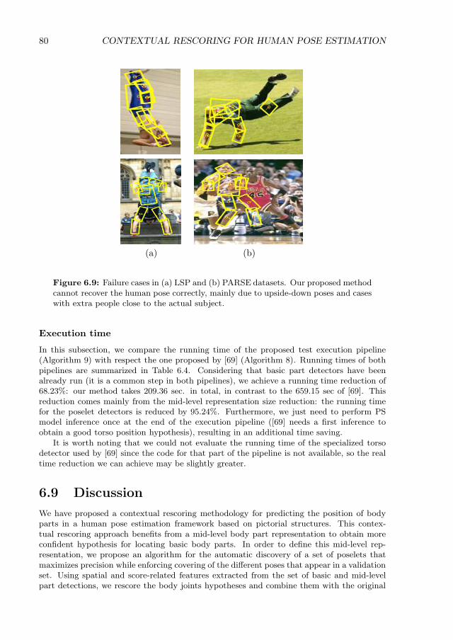
80 CONTEXTUAL RESCORING FOR HUMAN POSE ESTIMATION
(a) (b)
Figure 6.9: Failure cases in (a) LSP and (b) PARSE datasets. Our proposed methodcannot recover the human pose correctly, mainly due to upside-down poses and caseswith extra people close to the actual subject.
Execution time
In this subsection, we compare the running time of the proposed test execution pipeline(Algorithm 9) with respect the one proposed by [69] (Algorithm 8). Running times of bothpipelines are summarized in Table 6.4. Considering that basic part detectors have beenalready run (it is a common step in both pipelines), we achieve a running time reduction of68.23%: our method takes 209.36 sec. in total, in contrast to the 659.15 sec of [69]. Thisreduction comes mainly from the mid-level representation size reduction: the running timefor the poselet detectors is reduced by 95.24%. Furthermore, we just need to perform PSmodel inference once at the end of the execution pipeline ([69] needs a first inference toobtain a good torso position hypothesis), resulting in an additional time saving.
It is worth noting that we could not evaluate the running time of the specialized torsodetector used by [69] since the code for that part of the pipeline is not available, so the realtime reduction we can achieve may be slightly greater.
6.9 Discussion
We have proposed a contextual rescoring methodology for predicting the position of bodyparts in a human pose estimation framework based on pictorial structures. This contex-tual rescoring approach benefits from a mid-level body part representation to obtain moreconfident hypothesis for locating basic body parts. In order to define this mid-level rep-resentation, we propose an algorithm for the automatic discovery of a set of poselets thatmaximizes precision while enforcing covering of the different poses that appear in a validationset. Using spatial and score-related features extracted from the set of basic and mid-levelpart detections, we rescore the body joints hypotheses and combine them with the original

6.9. Discussion 81
0
0.02
0.04
0.06
0.08
0.1
0.12Upper limbs : 1. rel.y / 2. score.ratio / 3. rel.x
rel.x
rel.y
abs.r
el.x
abs.r
el.y
rel.w re
l.h
over
lap dist
scor
e.ra
tio
scor
e.dif
f0
0.02
0.04
0.06
0.08
0.1
0.12Lower limbs : 1. rel.x / 2. score.diff / 3. dist
rel.x
rel.y
abs.r
el.x
abs.r
el.y
rel.w re
l.h
over
lap dist
scor
e.ra
tio
scor
e.dif
f
(a) (b)
0
0.02
0.04
0.06
0.08
0.1
0.12Head & Torso : 1. rel.y / 2. rel.x / 3. score.diff
rel.x
rel.y
abs.r
el.x
abs.r
el.y
rel.w re
l.h
over
lap dist
scor
e.ra
tio
scor
e.dif
f0
0.02
0.04
0.06
0.08
0.1
0.12Full body : 1. rel.x / 2. rel.y / 3. score.ratio
rel.x
rel.y
abs.r
el.x
abs.r
el.y
rel.w re
l.h
over
lap dist
scor
e.ra
tio
scor
e.dif
f
(c) (d)
Figure 6.10: Contextual feature selection histograms computed from the learntdecision trees qθ, grouped by subsets of joints: (a) upper-body limbs, (b) lower-bodylimbs, (c) head & torso, and (d) full body.
Table 6.4: Running time (in seconds) of the test pipelines from [69] (Algorithm 8)and our proposal (Algorithm 9).
Steps Alg. 8 Alg. 9
1. Run PS model inference (torso hyp.) 148.70 -2. Run poselets 344.77 16.393. Run LDA/SetBoost classifiers 3.06 23.374. Run PS model inference 162.62 169.60
TOTAL 659.15 209.36
scores in the unary potential of a PS model.
Experiments with two standard benchmarks demonstrated that our body part positionprediction formulation can yield a performance similar to that of [69] in the LSP datasetand even better in the PARSE dataset, while reducing the number of poselets in the mid-level representation by 95.36%. Compared to other automatic poselet discovery strategies,the one proposed in this chapter yields the best results in combination with the proposedrescoring mechanism, in terms of PCP performance in the task of human pose estimation.

82 CONTEXTUAL RESCORING FOR HUMAN POSE ESTIMATION
(a) (b) (c) (d) (e)
Figure 6.11: Qualitative results on LSP dataset. (a) Gaussian-shaped positionprediction from [69], (b) Estimated pose from [69] (just predicting position), (c)Estimated pose from [69] (full model), (d) Position prediction with our proposedrescoring, and (e) Our results. White crosses in columns (a) and (d) show the partbeing rescored in each case; from the first row to the last one: rightmost ankle,rightmost wrist, leftmost ankle, leftmost wrist.
In addition, the proposed poselet discovery method is fully automatic, while the hierarchicaldecomposition from [69] is manually-defined.
In experiments that examined the influence of βup , the weight for the extra unary potential
that encodes position prediction based on poselet evidence, we noted that the results (PCP)are more stable with respect to changes βu
p , vs. [69]. Perhaps more crucially, the optimal

6.9. Discussion 83
(a) (b) (c) (d) (e)
Figure 6.12: Qualitative results on PARSE dataset. (a) Gaussian-shaped positionprediction from [69], (b) Estimated pose from [69] (just predicting position), (c)Estimated pose from [69] (full model), (d) Position prediction with our proposedrescoring, and (e) Our results. White crosses in columns (a) and (d) show the partbeing rescored in each case; from the first row to the last one: right ankle, right wrist,right ankle, left ankle.
value for βup is higher in our formulation vs. [69]: 0.45 vs. 0.15 for LSP, and 0.2 vs. 0.1 for
PARSE. This suggests that our proposed rescoring approach can produce a more reliableprediction of the part location in the image. A further analysis on the contextual featuresselected by the weak classifiers in the rescoring approach reveals that the most importantfeatures are the relative position and relative detection scores. This affirms that our methodcan discover patterns of the spatial layout of body parts and thus improve the body partlocalization obtained from the outputs of standard body part detectors.
Finally, we note that the reduction in the mid-level part representation results in a

84 CONTEXTUAL RESCORING FOR HUMAN POSE ESTIMATION
significant reduction in the execution time. We reduce the execution time by 68.23% withless than 2% reduction in accuracy w.r.t. the full model from [69]. Moreover, we just predictthe position of the body parts, while [69] also predicts their rotation and the pair-wiseparameters, and makes use of additional specialized head and torso detectors and a torsoposition prior.
As future work, we could adapt the proposed rescoring approach for predicting not onlythe position, but the rotation of the body parts. Additionally, we could extend the setof contextual features in order to directly model relative orientations between basic andmid-level parts through the contextual rescoring functions.

Part III
Gesture Recognition
85

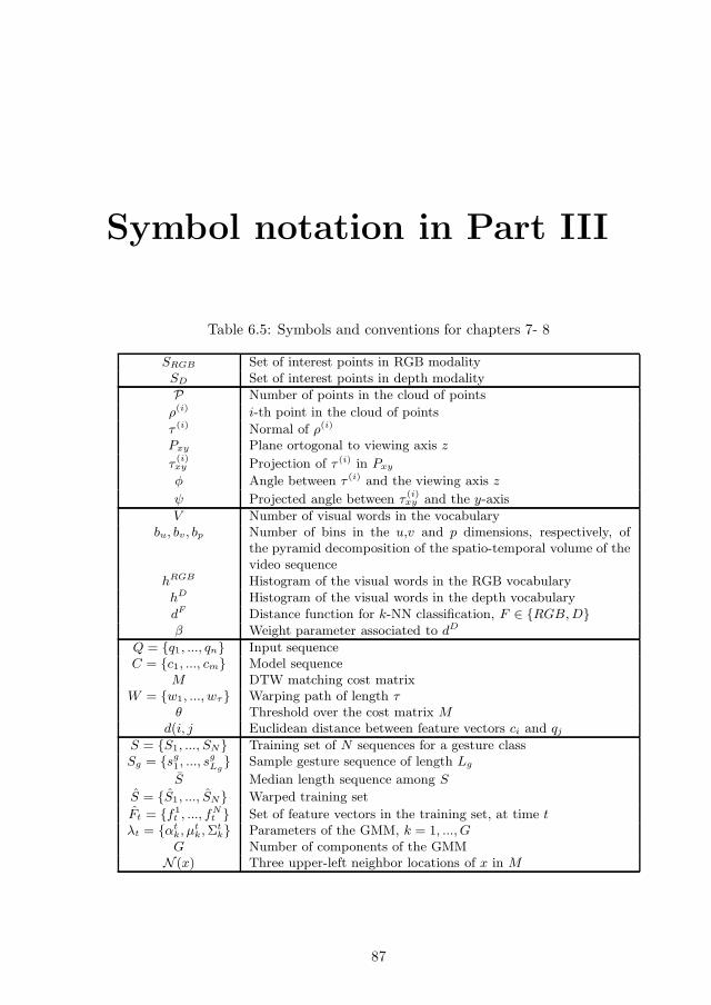
Symbol notation in Part III
Table 6.5: Symbols and conventions for chapters 7- 8
SRGB Set of interest points in RGB modalitySD Set of interest points in depth modality
P Number of points in the cloud of points
ρ(i) i-th point in the cloud of points
τ (i) Normal of ρ(i)
Pxy Plane ortogonal to viewing axis z
τ(i)xy Projection of τ (i) in Pxy
φ Angle between τ (i) and the viewing axis z
ψ Projected angle between τ(i)xy and the y-axis
V Number of visual words in the vocabularybu, bv, bp Number of bins in the u,v and p dimensions, respectively, of
the pyramid decomposition of the spatio-temporal volume of thevideo sequence
hRGB Histogram of the visual words in the RGB vocabularyhD Histogram of the visual words in the depth vocabularydF Distance function for k-NN classification, F ∈ RGB,Dβ Weight parameter associated to dD
Q = q1, ..., qn Input sequenceC = c1, ..., cm Model sequence
M DTW matching cost matrixW = w1, ..., wτ Warping path of length τ
θ Threshold over the cost matrix Md(i, j Euclidean distance between feature vectors ci and qj
S = S1, ..., SN Training set of N sequences for a gesture classSg = sg1, ..., s
gLg
Sample gesture sequence of length Lg
S Median length sequence among S
S = S1, ..., SN Warped training set
Ft = f1t , ..., f
Nt Set of feature vectors in the training set, at time t
λt = αtk, µ
tk,Σ
tk Parameters of the GMM, k = 1, ..., G
G Number of components of the GMMN (x) Three upper-left neighbor locations of x in M
87

88

Chapter 7
BoVDW for gesture recognition
7.1 Introduction
Gestures play an important role in human communication. We use them naturally in ourdaily lives, from linguistic to artistic points of view, including for example referee signalsin sports, gestures to accompany speech or sign language for the deaf. More specifically,a gesture is a form of non-verbal communication involving the movement of some parts ofthe body (being usually the arms and the hands the most used ones), with the purpose ofexpressing a sign or an action with a specific meaning.
Gestures take place in the spatio-temporal domain, given that they imply a movementof the body parts among the 3-D spatial coordinates, during a specific amount of time.Therefore, a gesture is delimited by a “beginning” and an “end” time instants. In theComputer Vision field, gesture recognition methodologies typically distinguish two steps:gesture segmentation, and gesture recognition per se. Usually, gesture segmentation is firstlyperformed to find the “beginning” and “end” of the gestures performed in a video sequence.Then, gesture recognition is defined as a classification step in which a gesture label is assignedto a given time segment, previously found in the gesture segmentation step.
Human gesture recognition is one of the most challenging tasks in computer vision.Current methodologies have shown preliminary results on very simple scenarios, but they arestill far from human performance. Due to the large number of potential applications involvinghuman gesture recognition in fields like surveillance [45], sign language recognition [80],or clinical assistance [67] among others, there is a large and active research communitydevoted to deal with this problem. Independently of the application field, the usual humangesture recognition pipeline is mainly formed by two steps: gesture representation and gestureclassification.
In this chapter we introduce a Bag-of-Visual-and-Depth-Words (BoVDW) representationfor gestures, as an extension of the Bag-of-Visual-Words (BoVW) that fuses informationfrom multi-modal RGBD data streams. Regarding gesture classification, we address theproblem of one-shot human gesture recognition, i.e. at training time just one gesture sampleis available, for each gesture class we want to recognize.
In order to evaluate the presented approach, we compare the performances achievedwith state-of-the-art RGB and depth feature descriptors separately, and combine them ina late fusion fashion. All the experiments are performed in the proposed framework using
89

90 BOVDW FOR GESTURE RECOGNITION
the public data set provided by the ChaLearn Gesture Challenge1. Results of the proposedBoVDW method show better performance using late fusion in comparison to early fusionand standard BoVW model. Moreover, our BoVDW approach outperforms the baselinemethodology provided by the ChaLearn Gesture Challenge 2012.
7.2 Related work
When it comes to representing gestures, literature shows a variety of methods that haveobtained successful results. Commonly applied in image retrieval or image classificationscenarios, Bag-of-Visual-Words (BoVW) is one of the most used approaches. This method-ology is an evolution of Bag-of-Words (BoW) [60] representation, used in document analysis,where each document is represented using the frequency of appearance of each word in adictionary. In the image domain, these words become visual elements of a defined visual vo-cabulary. First, each image is decomposed into a large set of patches, either using some typeof spatial sampling (grids, sliding window, etc.) or detecting points with relevant properties(corners, salient regions, etc.). Each patch is then described obtaining a numeric descriptor.A set of V representative visual words are selected by means of a clustering process over thedescriptors. Once the visual vocabulary is defined, each new image can be represented by aglobal histogram containing the frequencies of visual words. Finally, this histogram can beused as input for any classification technique (i.e. k−Nearest Neighbor or SVM) [29, 64]. Inaddition, extensions of BoVW from still images to image sequences have been recently pro-posed in the context of human action recognition, defining Spatio-Temporal-Visual-Words(STVW) [65].
As commented in chapters 1 and 4, the release of the Microsoft KinectTM sensor in late2010 has allowed an easy and inexpensive access to almost synchronized range imaging withstandard video data. Those data combine both sources into what is commonly named RGBDimages (RGB plus Depth). This multi-modal data has reduced the burden of the first stepsin many pipelines devoted to image or object segmentation, and opened new questions suchas how these data can be effectively described and fused. Motivated by the informationprovided by depth maps, several 3-D descriptors have been recently developed [14, 75] (mostof them based on codifying the distribution of normal vectors among regions in the 3D space),as well as their fusion with RGB data [56] and learning approaches for object recognition [13].This depth information has been particularly exploited for gesture recognition and humanbody segmentation and tracking. While some works focus on just the hand regions forperforming gesture recognition [12, 34, 54, 61, 66, 89], in [79] Shotton et al . introduced oneof the greatest advances in the extraction of the human body pose using RGBD, whichis provided as part of the KinectTM human recognition framework. The method is basedon inferring pixel label probabilities through Random Forest from learned offsets of depthfeatures. Then, mean shift is applied to estimate human joints and representing the bodyin skeletal form. In chapter 4 we extended Shotton et al .’s work applying Graph-cuts to thepixel label probabilities obtained through Random Forest, in order to compute consistentsegmentations in the spatio-temporal domain. Girshick et al . [43] proposed later a differentapproach in which they directly regress the positions of the body joints, without the need ofan intermediate pixel-wise body limb classification as in [79]. The extraction of body poseinformation opens the door to one of the most challenging problems nowadays, i.e. humangesture recognition.
Recently, many works have been proposed based on the skeletal models provided byRGB-D devices like KinectTM .Wu et al . [93] presents a method that combines the output
1http://gesture.chalearn.org/

7.3. Bag of Visual Words 91
of two different classifiers to perform gesture recognition. The first classifier is based onskeletal features whole the second receives audio features as input. Finally, in order toprovide a global score for a video sequence to be labeled as a given gesture, the outputsof both classifiers are weighted. A similar approach is presented by Bayer et al . [11]: theauthors perform model averaging by assigning different weights to classifiers over audio andskeleton-based features.
More similarly to the methodology we propose, other works in the state of the art combinedifferent visual modalities like RGB images and depth maps (a.k.a. RGBD images) providedby Kinect sensors to perform gesture recognition. In [84] the authors propose a combinationof Histograms of Oriented Gradients (HOG) features extracted from RGB and depth images,using as keypoints the joints from the retrieved skeleton model of the person. In [23] theauthors concatenate HOG features extracted from the image regions around each hand withfeatures extracted from the skeletal models retrieved by Kinect. In total, they fuse threedifferent features: HOG for the hand regions, normalized 3-D coordinates of the skeletonkeypoints, and pairwise skeleton distances among keypoints. In addition, the authors alsopropose a late fusion approach to combine the classification outputs of when concatenatingdifferent subsets of features, as well as the concatenation of all three features.
7.3 Bag of Visual Words
Bag of visual words is the extension of the bag of words representation, used to capturethe semantics of the words in a text, to the image domain. The original bag of wordsrepresentation is depicted in Fig. 7.1(a). Basically, it consists on a histogram that capturesthe appearance frequency of a set of words in a given vocabulary, over a whole document.While the ordering of the words in the text is lost in such histogram-based representation,it is expected to capture higher-level semantics: problems like spam filtering (i.e. classifyinge-mails as spam or not), or newspaper article classification, have been successfully addressedusing bag of words representation.
When extending the bag of words representation to the image domain, the concepts ofvisual words and visual vocabulary are introduced. In the text domain, we naturally detectwords and identify them given a vocabulary, e.g . an English dictionary. Following the sameidea, a visual word is defined as a small patch in an image, which can be identified in a givenvisual vocabulary or codebook, i.e. a set of visual words. In practice, defining the visualvocabulary is performed in an unsupervised fashion, following the next pipeline:
1. Keypoint detection: Given a set of images, a set of interest points are detected, e.g .Harris [46], SIFT [63], or a dense grid detector. These interest points are commonlyparametrized as oriented circular patches of a given radius.
2. Keypoint description: Given a detected interest point and its corresponding imagepatch, a feature vector (e.g . SIFT [63] ,HOG [30]) is computed, and stored for furtherprocessing.
3. Codebook generation: In order to define the visual vocabulary or codebook, aquantization step is performed over the feature vectors, previously extracted from aset of images. One simple yet commonly used method for codebook generation isk-means clustering: given a number of visual words k and a set of feature vectors,k-means partitions the feature space into k clusters or visual words.
Once the visual codebook is generated, an image can be represented as a histogramof visual words by first detecting a set of interest points and extracting the same featurevectors used for the generation of the codebook. Then, each interest point can be identified
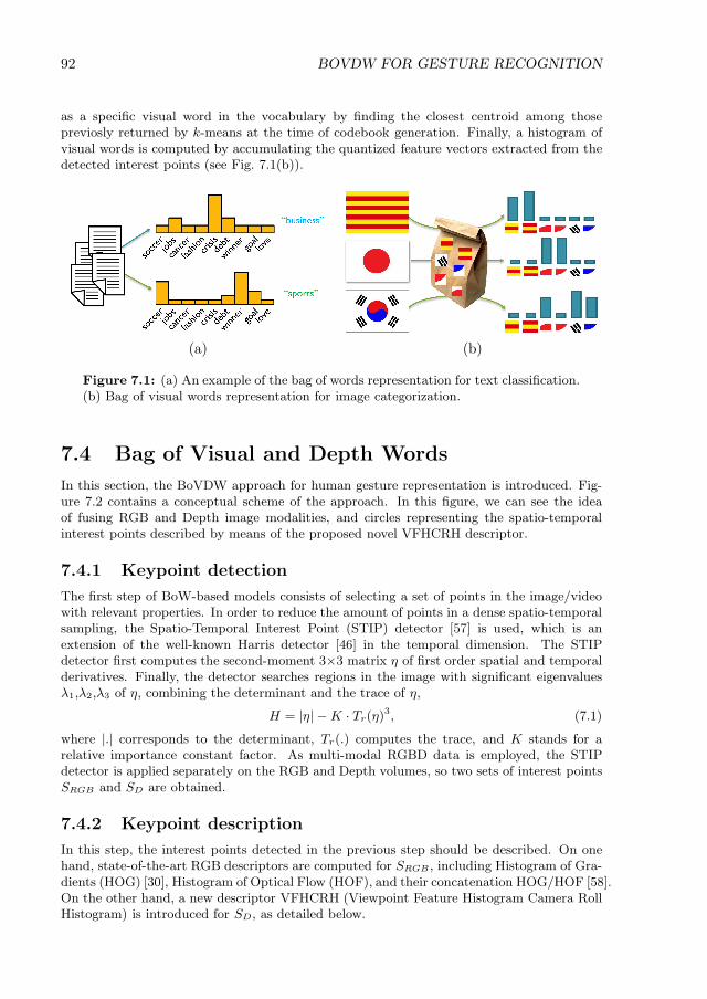
92 BOVDW FOR GESTURE RECOGNITION
as a specific visual word in the vocabulary by finding the closest centroid among thosepreviosly returned by k-means at the time of codebook generation. Finally, a histogram ofvisual words is computed by accumulating the quantized feature vectors extracted from thedetected interest points (see Fig. 7.1(b)).
(a) (b)
Figure 7.1: (a) An example of the bag of words representation for text classification.(b) Bag of visual words representation for image categorization.
7.4 Bag of Visual and Depth Words
In this section, the BoVDW approach for human gesture representation is introduced. Fig-ure 7.2 contains a conceptual scheme of the approach. In this figure, we can see the ideaof fusing RGB and Depth image modalities, and circles representing the spatio-temporalinterest points described by means of the proposed novel VFHCRH descriptor.
7.4.1 Keypoint detection
The first step of BoW-based models consists of selecting a set of points in the image/videowith relevant properties. In order to reduce the amount of points in a dense spatio-temporalsampling, the Spatio-Temporal Interest Point (STIP) detector [57] is used, which is anextension of the well-known Harris detector [46] in the temporal dimension. The STIPdetector first computes the second-moment 3×3 matrix η of first order spatial and temporalderivatives. Finally, the detector searches regions in the image with significant eigenvaluesλ1,λ2,λ3 of η, combining the determinant and the trace of η,
H = |η| −K · Tr(η)3, (7.1)
where |.| corresponds to the determinant, Tr(.) computes the trace, and K stands for arelative importance constant factor. As multi-modal RGBD data is employed, the STIPdetector is applied separately on the RGB and Depth volumes, so two sets of interest pointsSRGB and SD are obtained.
7.4.2 Keypoint description
In this step, the interest points detected in the previous step should be described. On onehand, state-of-the-art RGB descriptors are computed for SRGB , including Histogram of Gra-dients (HOG) [30], Histogram of Optical Flow (HOF), and their concatenation HOG/HOF [58].On the other hand, a new descriptor VFHCRH (Viewpoint Feature Histogram Camera RollHistogram) is introduced for SD, as detailed below.

7.4. Bag of Visual and Depth Words 93
Figure 7.2: BoVDW approach in a Human Gesture Recognition scenario. Interestpoints in RGB and depth images are depicted as circles. Circles indicate the assign-ment to a visual word in the shown histogram – computed over one spatio-temporalbin. Limits of the bins from the spatio-temporal pyramids decomposition are repre-sented by dashed lines in blue and green, respectively. A detailed view of the normalsof the depth image is shown in the upper-left corner.
VFHCRH
The recently proposed Point Feature Histogram (PFH) and Fast Point Feature Histogram(FPFH) descriptors [14] represent each instance in the 3-D cloud of points with a histogramencoding the distribution of the mean curvature around it. Both PFH and FPFH provideP6 DOF (Degrees of Freedom) pose invariant histograms, being P the number of pointsin the cloud. Following their principles, Viewpoint Feature Histogram (VFH)[75] describeseach cloud of points with one descriptor of 308 bins, variant to object rotation around pitchand yaw axis. However, VFH is invariant to rotation about the roll axis of the camera.In contrast, Clustered Viewpoint Feature Histogram (CVFH) [8] describes each cloud ofpoints using a different number of descriptors r, where r is the number of stable regionsfound on the cloud. Each stable region is described using a non-normalized VFH histogramand a Camera’s Roll Histogram (CRH), and the final object description includes all regiondescriptors. CRH is computed by projecting the normal of the point cloud τ (i) of the i-thpoint ρ(i) onto a plane Pxy that is orthogonal to the viewing axis z, the vector between thecamera center and the centroid of the cloud, under orthographic projection,
τ (i)xy = ||τ (i)|| · sin(φ), (7.2)
where φ is the angle between the normal τ (i) and the viewing axis. Finally, the histogramencodes the frequencies of the projected angle ψ between τ
(i)xy and y-axis, the vertical vector
of the camera plane (see Fig. 7.3(a)).In order to avoid descriptors of arbitrary lengths for different point clouds, the whole

94 BOVDW FOR GESTURE RECOGNITION
(a) (b)
Figure 7.3: (a) Point cloud of a face and the projection of its normal vectors onto theplane Pxy , orthogonal to the viewing axis z. (b) VFHCRH descriptor: Concatenationof VFH and CRH histograms resulting in 400 total bins
cloud is described using VFH. In addition, a 92 bins CRH is computed for encoding 6DOF information. The concatenation of both histograms results in the proposed VFHCRHdescriptor of 400 bins shown in Figure 7.3(b). Note how the first 308 bins of the concatenatedfeature vector correspond to the VFH, that encode the normals of the point cloud. Finally,the remaining bins corresponding to the CRH descriptor, encode the information of therelative orientation of the point cloud to the camera.
7.4.3 BoVDW histogram
Once all the detected points have been described, the vocabulary of V visual/depth wordsis designed by applying a clustering method over all the descriptors. Hence, the clusteringmethod –k-means in our case– defines the words from which a query video sequence will berepresented, shaped like a histogram h that counts the appearance frequency of each word.Additionally, in order to introduce geometrical and temporal information, spatio-temporalpyramids are applied, following the work of Lazebnik et al . [59]. Basically, spatio-temporalpyramids consist of dividing the video volume in bx, by , and bt bins along the spatial x andv dimensions, and the temporal dimension t of the volume. Then, bx × by × bt separatehistograms are computed with the points lying in each one of these bins, and they areconcatenated jointly with the general histogram computed using all points.
These histograms define the model for a certain class of the problem –in our case, acertain gesture. Since multi-modal data is considered, different vocabularies are defined forthe RGB-based descriptors and the depth-based ones, and the corresponding histograms,hRGB and hD, are obtained. Finally, the information given by the different modalities ismerged in the next and final classification step, hence using late fusion.
7.4.4 BoVDW-based classification
The final step of the BoVDW approach consists of predicting the class of a query video.For that, any kind of multi-class supervised learning technique could be used. In our case,a simple k-Nearest Neighbour classification is used, computing the complementary of the

7.5. Experiments 95
histogram intersection as a distance,
dF = 1−∑
i
min(hFmodel(i), h
Fquery(i)), (7.3)
where F ∈ RGB,D. Finally, in order to merge the histograms hRGB and hD, the distancesdRGB and dD are computed separately, as well as the weighted sum,
dhist = (1− β)dRGB + βdD, (7.4)
to perform late fusion, where β is a weighting factor.
7.5 Experiments
In this section we evaluate the proposed BoVDW framework for one-shot gesture recognition,comparing different state-of-the-art descriptors in both RGB and depth image modalities.We first present the dataset used in the performed experiments, provided by the ChaLearnGesture Challenge organization [22]. Next, parameters and evaluation measures are dis-cussed, and finally we show quantitative results of the proposed method.
7.5.1 Data
For the experimental evaluation, we used the ChaLearn [22] data set, provided by theCVPR2012 Workshop’s challenge on Human Gesture Recognition. The data set consists of50, 000 gestures each one portraying a single user in front of a fixed camera. The images arecaptured by a Kinect device providing both RGB and depth images. A subset of the wholedata set has been considered, formed by 20 development batches with a manually taggedgesture segmentation. Each batch includes 100 recorded gestures grouped in sequences of 1to 5 gestures performed by the same user. The gestures from each batch are drawn from adifferent lexicon of 8 to 15 unique gestures and just one training sample per gesture is pro-vided. These lexicons are categorized in nine classes, including: (1) body language gestures(scratching your head, crossing your arms, etc.), (2) gesticulations performed to accompanyspeech, (3) illustrators (like Italian gestures), (4) emblems (like Indian Mudras), (5) signs(from sign languages for the deaf), (6) signals (diving signals, mashalling signals to guidemachinery or vehicle, etc.), (7) actions (like drinking or writing), (8) pantomimes (gesturesmade to mimic actions), and (9) dance postures.
7.5.2 Methods and validation
In all the experiments shown in this section, the vocabulary size was set to V = 200 wordsfor both RGB and depth cases. For the spatio-temporal pyramids, the volume was dividedin 2 × 2 × 2 bins (resulting in a final histogram of 1800 bins). Since the nature of ourapplication problem is one-shot learning (only one training sample is available for each class),a simple Nearest Neighbor classification is employed. Finally, for the late fusion, the weightβ = 0.8 was empirically set, by testing the performance of our method in a small subset ofdevelopment batches from the dataset. We observed that when increasing β, starting fromβ = 0, the performance keeps increasing in a linear fashion, until the value β = 0.45. Fromβ = 0.45 to β = 0.8 the performance keeps improving more slowly, and finally, from β = 0.8to β = 1 the performance drops again.
For the evaluation of the methods, in the context of Human Gesture Recognition, theLevenshtein distance or edit distance was considered. This edit distance between two strings

96 BOVDW FOR GESTURE RECOGNITION
Table 7.1: Mean Levenshtein distance for RGB and depth descriptors.
RGB desc. MLD Depth desc. MLD
HOG 0.3452 VFH 0.4021HOF 0.4144 VFHCRH 0.3064
HOGHOF 0.3314
is defined as the minimum number of operations (insertions, substitutions or deletions)needed to transform one string into the other. In our case, strings contain the gesture classlabels detected in a video sequence. For all the comparison, the Mean Levenshtein distance(MLD) was computed over all sequences and batches.
7.5.3 Results
Table 7.1 shows a comparison between different state-of-the-art RGB and depth descriptors(including our proposed VFHCRH), using our BoVDW approach. Moreover, we compareour BoVDW framework with the baseline methodology provided by the ChaLearn 2012Gesture Recognition challenge. This baseline first computes an average movement image foreach gesture class by computing the mean value for each pixel in the image, along the timedimension. Then, the classification of a new gesture is basically performed by means of aNearest Neighbor classifier computing the Euclidean distance between the average movementimage from the query gesture and the templates in the training database. This baselineobtains a MLD of 0.5096. Table 7.2 shows the results in all the 20 development batchesseparately.
When using our BoVDW approach, in the case of RGB descriptors, HOF alone performsthe worst. In contrast, the early concatenation of HOF to HOG descriptor outperformsthe simple HOG. Thus, HOF contributes adding discriminative information to HOG. Ina similar way, looking at the depth descriptors, it can be seen how the concatenation ofthe CRH to the VFH descriptor clearly improves the performance compared to the simplerVFH. When using late fusion in order to merge information from the best RGB and depthdescriptors (HOGHOF and VFHCRH, respectively), a value of 0.2714 for MLD is achieved.Figure 7.4 shows the confusion matrices of the gesture recognition results with this late fusionconfiguration. In general, the confusion matrices follow an almost diagonal shape, indicatingthat the majority of the gestures are well classified. However, the results of batches 3, 16, 18,19 are significantly worse, possibly due to the static characteristics of the gestures in thesebatches. Furthermore, late fusion was also applied in a 3-fold way, merging HOG, HOF,and VFHCRH descriptors separately. In this case the weight β was assigned to HOG andVFHCRH descriptors (and 1− β to HOF), improving the MLD to 0.2662. From this resultit can be concluded that HOGHOF late fusion performs better than HOGHOF early fusion.
7.6 Discussion
We presented the BoVDW approach for Human Gesture Recognition, using multi-modalRGBD video sequences. A new depth descriptor VFHCRH has been proposed, which out-performs simpler VFH, in the task of gesture recognition. Moreover, the effect of the latefusion has been analyzed for the combination of RGB and depth descriptors in the BoVDW,obtaining better performance in comparison to early fusion.

7.6. Discussion 97
Figure 7.4: Confusion matrices for gesture recognition in each one of the 20 devel-opment batches.
Among the different RGB descriptors included in the comparison, we showed that theconcatenation of HOG and HOF is the one yielding the best results. Moreover, we showhow the concatenation of VFH and CRH descriptors outperform VFH in the case of depthdescriptors. Generally speaking, the best scoring depth descriptor (VFHCRH) by itselfobtains better results than the best one from the RGB stream (HOGHOF). Hence, whenusing late fusion to merge information from both RGB and Depth video streams, we not

98 BOVDW FOR GESTURE RECOGNITION
Table 7.2: Mean Levenshtein Distance of the best RGB and depth descriptorsseparately, as well as the 2-fold and 3-fold late fusion of them. Results obtained bythe baseline from the ChaLearn challenge are also shown. Rows 1 to 20 representthe different batches.
HOGHOF VFHCRH 2-fold L.F. 3-fold L.F. Baseline
1 0.19 0.17 0.12 0.20 0.422 0.24 0.30 0.24 0.26 0.573 0.76 0.39 0.40 0.49 0.784 0.14 0.08 0.08 0.11 0.325 0.08 0.33 0.17 0.17 0.256 0.41 0.47 0.44 0.34 0.547 0.10 0.18 0.11 0.13 0.648 0.12 0.26 0.14 0.08 0.409 0.11 0.18 0.15 0.13 0.3010 0.57 0.40 0.39 0.46 0.7911 0.47 0.36 0.27 0.34 0.5412 0.37 0.20 0.21 0.17 0.4213 0.16 0.14 0.10 0.09 0.3414 0.41 0.34 0.30 0.30 0.6915 0.38 0.28 0.34 0.28 0.5416 0.22 0.41 0.34 0.29 0.4217 0.38 0.16 0.15 0.17 0.5518 0.38 0.43 0.40 0.38 0.5319 0.67 0.50 0.50 0.44 0.6120 0.46 0.57 0.56 0.48 0.52
Mean 0.3314 0.3064 0.2714 0.2662 0.5096
surprisingly discover that the best value for β favors depth words in front of those fromthe RGB vocabulary. Not only that, but we also show that building different vocabulariesfor HOG and HOF separately and merging their information at the histogram level (latefusion) yields better results than building just one vocabulary over the concatenation ofboth descriptors (early fusion).
An additional advantage of using late fusion w.r.t early fusion is the flexibility of themodel upon possible extensions. Adding an additional set of features to an existing modelin an early fusion fashion, implies to generate a new codebook or visual vocabulary, andtherefore, re-train the whole system from blank. In contrast, by keeping different vocabulariesfor each feature we want to include in the system, i.e. when using late fusion, we are able toadd new features to the by just computing a new vocabulary while the vocabularies for thefeatures already computed remain the same. In addition, we can define different cardinalitiesfor each visual vocabulary, allowing for a more flexible formulation of the model.
As further research on the topic, it would be interesting to study the behavior of latefusion when adding more descriptors to the framework, and studying ways to optimize thecorresponding weights of each visual vocabulary.

Chapter 8
PDTW for continuous gesture
recognition
8.1 Introduction
In the previous chapter we presented a method for representing and classifying gestures,by computing a bag-of-visual-and-depth-words descriptor over a spatio-temporal volumecorresponding to an RGBD multimodal video sequence, where a person standing in front ofthe camera is performing one gesture. While we show successful results in gesture recognitionwith this methodology, we assume that we know the beginning and the end time frames thatdelimit the gestures performed by the actor. However, in many computer vision applicationsrelated to gesture recognition, we do not have such beginning/end labels available, so priortemporal segmentation of the gestures should be performed in order to obtain the spatio-temporal volumes containing isolated gestures. Then, the corresponding bag-of-visual-and-depth-words feature vectors can be computed for each volume, and final classification isperformed independently for each isolated gesture.
On the other hand, other methods try to directly recognize gestures in a continuous inputstream, i.e. continuous gesture recognition. The problem of continuous gesture recognition isaddressed in this chapter: we introduce an extension of the DTW method to a probability-based framework able to capture the intra-class variability of each gesture class. In theexperimental section, we show quantitative and qualitative results on the ChaLearn GestureChallenge dataset [22]. We apply the proposed method to recognize the “idle” or referencegesture, performed by the actors between the end of a gesture and the beginning of the nextone, i.e. we perform temporal gesture segmentation.
8.2 Related work
Methods based on dynamic programming algorithms for both alignment and clustering oftemporal series [98] are commonly used for continuous gesture recognition. In addition,other probabilistic methods such as Hidden Markov Models (HMM) or Conditional RandomFields (CRF) have been also commonly used in the literature [80]. Nevertheless, one ofthe most common methods for continuous human gesture recognition is Dynamic TimeWarping (DTW) [9, 72], since it offers a simple yet effective temporal alignment betweensequences of different lengths. However, the application of such methods to gesture detection
99

100 PDTW FOR CONTINUOUS GESTURE RECOGNITION
in complex scenarios becomes a hard task due to the high variability of the environmentalconditions among different domains. Some common problems are: wide range of humanpose configurations, influence of background, continuity of human movements, spontaneityof human actions, speed, appearance of unexpected objects, illumination changes, partialocclusions, or different points of view, just to mention a few. These effects can cause dramaticchanges in the description of a certain gesture, generating a great intra-class variability. Inthis sense, since usual DTW is applied between a sequence and a single pattern, it fails whentaking into account such variability.
8.3 Dynamic Time Warping
The original DTW is introduced in this section, as well as its common extension to detect acertain sequence given an indefinite data stream.
The original DTW algorithm was defined to match temporal distortions between twomodels, finding an alignment/warping path between two time series: an input model Q =q1, .., qn and a certain sequence C = c1, .., cm. In our particular case, the time seriesQ and C are video sequences, where each qj and ci will be feature vectors describing thej−th and i−th frame respectively. In this sense, Q will be an input video sequence andC will be the model gesture we are aiming to detect. Generally, in order to align thesetwo sequences, a Mm×n matrix is designed, where position (i, j) of the matrix contains thealignment cost between ci and qj . Then, a warping path of length τ is defined as a set ofcontiguous matrix elements, defining a mapping between C and Q: W = w1, .., wτ, wherewi indexes a position in the cost matrix M . This warping path is typically subject to severalconstraints,
• Boundary conditions: w1 = (1, 1) and wτ = (m,n).
• Continuity and monotonicity: Given wτ ′−1 = (a′, b′), wτ ′ = (a, b), then a−a′ ≤ 1and b − b′ ≤ 1. This condition forces the points in the cost matrix with the warpingpath W to be monotonically spaced in time.
Interest is focused on the final warping path that, satisfying these conditions, minimizesthe warping cost,
DTW (M) = minW
M(wτ )
τ
, (8.1)
where τ compensates the different lengths of the warping paths at each time t. This pathcan be found very efficiently using dynamic programming. The cost at a certain positionM(i, j) can be found as the composition of the Euclidean distance d(i, j) between the featurevectors ci and qj of the two time series, and the minimum cost of the adjacent elements ofthe cost matrix up to that position, as,
M(i, j) = d(i, j) +minM(i− 1, j − 1),M(i− 1, j),M(i, j − 1). (8.2)
However, given the streaming nature of our problem, the input video sequence Q has nodefinite length (it may be an infinite video sequence) and may contain several occurrencesof the gesture sequence C. In this sense, the system considers that there is correspondencebetween the current block k in Q and the gesture when the following condition is satisfied,M(m, k) < θ, k ∈ [1, ..,∞] for a given cost threshold θ. At this point, if M(m,k) < θ k isconsider a possible end of a gesture sequence C.
Once detected a possible end of the gesture sequence, the warping path W can be foundthrough backtracking the minimum cost path from M(m, k) to M(0, g), being g the instantof time in Q where the detected gesture begins. Note that d(i, j) is the cost function which

8.4. Handling variance with Probability-based DTW 101
IDLE GESTURE
DESCRIPTION
IDLE GESTURE
ALIGNMENTGMM LEARNING
PROBABILISTIC
DTW
λN
ωN
k, µN
k,ΣN
k, i ∈ [1, 2, 3]
DTW
1 ∞
L
+
HOG HOF
GESTURE SAMPLES
ALIGNED GESTURE
SAMPLES
Figure 8.1: Flowchart of the Probabilistic DTW gesture segmentation methodology.
measures the difference among descriptors ci and qj , which in standard DTW is defined asthe euclidean distance between ci and qj . An example of a begin-end gesture recognitiontogether with the warping path estimation is shown in Figure 8.1 (last 2 steps: GMM learningand Probabilistic DTW).
8.4 Handling variance with Probability-based DTW
In this section, DTW is extended in order to align patterns taking into account the probabilitydensity function (PDF) of each element of the sequence by means of a Gaussian MixtureModel (GMM). A flowchart of the whole methodology is shown in Figure 8.1.
Consider a training set of N sequences, S = S1, . . . , Sg, . . . , SN, that is, N gesture sam-ples belonging to the same gesture category. Then, each sequence Sg = sg1, . . . , s
gt , . . . , s
gLg
,
(each gesture sample) is composed by a feature vector 1 for each frame t, denoted as sgt , whereLg is the length in frames of sequence Sg. In order to avoid temporal deformations of thegesture samples in S, all sequences are aligned with the median length sequence using theclassical DTW with Euclidean distance. Let us assume that sequences are ordered accordingto their length, so that Lg−1 ≤ Lg ≤ Lg+1, ∀g ∈ [2, .., N − 1], then, the median lengthsequence is S = S⌈N
2⌉.
It is worth noting that this alignment step by using DTW has no relation to the actualgesture recognition, as it is considered a pre-processing step to obtain a set of gesture sampleswith few temporal deformations and a matching length.
Finally, after this alignment process, all sequences have length L⌈N2⌉. The set of warped
sequences is defined as S = S1, S2, . . . , SN (See Figure 8.2(b)). Once all samples arealigned, the N feature vectors corresponding to each sequence element at a certain framet, denoted as Ft = f1
t , f2t , ..., f
Nt , are modelled by means of a G−component Gaussian
Mixture Model (GMM) λt = αtk, µ
tk,Σ
tk, k = 1, . . . , G, where αt
k is the mixing value,
1HOG/HOF descriptors in our particular case, see Sec. 8.5 for further details.

102 PDTW FOR CONTINUOUS GESTURE RECOGNITION
Mean length sample
Warped Sequences
F1
FL⌈N
2⌉
(a)(b)
(c) (d)
S
SN
λN
ωN
k, µN
k,ΣN
k, i ∈ [1, 2, 3]
λ1
ω1
k, µ1
k,Σ1
k, i ∈ [1, 2, 3]
S1
S
S1
SN
DTW
S1
SN
Figure 8.2: (a) Different sequences of a certain gesture category and the medianlength sequence. (b) Alignment of all sequences with the median length sequence bymeans of Euclidean DTW. (c) Warped sequences set S from which each set of t-thelements among all sequences are modelled. (d) Gaussian Mixture Model learningwith 3 components.
and µtk and Σt
k are the parameters of each of the G Gaussian models in the mixture. As aresult, each one of the GMMs that model each Ft is defined as follows,
p(Ft) =
G∑
k=1
αtk · e−
12(x−µt
k)T ·(Σt
k)−1·(x−µtk). (8.3)
The resulting model is composed by the set of GMMs that model each set Ft among allwarped sequences of a certain gesture class. An example of the process is shown in Figure8.2.

8.5. Experiments 103
8.4.1 Distance measures
In the classical DTW, a pattern and a sequence are aligned using a distance metric, suchas the Euclidean distance. However, since our gesture samples are modelled by means ofprobabilistic models, in order to use the principles of DTW, the distance must be redefined.In this sense, a soft-distance based on the probability of a point x belonging to each one ofthe G components in the GMM is considered, i.e. the posterior probability of x is obtained
according to Eq. (8.3). Therefore, sinceG∑
k=1
αtk = 1, the probability of a element qj ∈ Q
belonging to the whole GMM λt can be computed as,
P (qj , λt) =G∑
k=1
αtk · P (qj)k, (8.4)
P (qj)k = e−12(qj−µt
k)T ·(Σtk)
−1·(qj−µtk), (8.5)
which is the sum of the weighted probability of each component. Nevertheless, an additionalstep is required since the standard DTW algorithm is conceived for distances instead ofsimilarity measures. In this sense, a soft-distance based measure of the probability is used,which is defined as,
D(qj , λt) = exp−P (qj ,λt) . (8.6)
In conclusion, possible temporal deformations of different samples of the same gesturecategory are taken into account by aligning the set of N gesture samples with the medianlength sequence. In addition, by modelling each set of feature vectors which compose theresulting warped sequences with a GMM, we obtain a methodology for gesture detection thatis able to deal with multiple deformations in gestures both temporal (which are modelledby the DTW alignment), or descriptive (which are learned by the GMM modelling). Thealgorithm that summarizes the use of the probability-based DTW to detect start-end ofgesture categories is shown in Table 10. Figure 8.3 illustrates the application of the algorithmin a toy problem.
8.5 Experiments
In this section we provide with quantitative and qualitative evaluation of the proposed proba-bilistic dynamic time warping methodology, in the context of continuous gesture recognition.More specifically, we aim to detect an “idle” or resting gesture performed by the actors inthe ChaLearn Gesture Challenge dataset, between labeled gestures in the video sequences.Hence, detecting the “idle” gesture between other gestures of interest can be understood asgesture segmentation. We start by presenting the data we used for the experiments, thenwe detail the experimental settings, and finally present quantitative and qualitative resultsfor the proposed gesture segmentation application.
8.5.1 Data
For the temporal gesture segmentation experiments we used the 20 development batchesprovided by the organization of the ChaLearn Gesture Challenge 2012 [22], as in the previouschapter of this thesis. These batches contain a manual labelling of gesture start and endpoints. Each batch includes 100 recorded gestures, grouped in sequences of 1 to 5 gesturesperformed by the same user. For each sequence the actor performs an idle gesture betweeneach gesture of the gestures drawn from lexicons. Finally, this means that we have a set ofapproximately 1, 800 idle gesture samples.

104 PDTW FOR CONTINUOUS GESTURE RECOGNITION
Algorithm 10 Probability-based DTW algorithm.
Input: A set of GMM models λ = λ1, .., λm corresponding to a gesture cat-egory, a threshold value θ, and the streaming sequence Q = q1, .., q∞. Costmatrix Mm×∞ is defined, where N (x), x = (i, t) is the set of three upper-leftneighbor locations of x in M .Output: Warping path W of the detected gesture, if any.
1: for i = 1 : m do2: for j = 1 :∞ do3: M(i, j) =∞4: end for5: end for6: for j = 1 :∞ do7: M(0, j) = 07:
8: end for9: for j = 0 :∞ do
10: for i = 1 : m do11: x = (i, j)12: M(x) = D(qj , λi) + min
x′∈N (x)M(x′)
13: end for14: if M(m, j) < θ then15: W = argmin
x′∈N (x)
M(x′)
16: return17: end if18: end for
8.5.2 Methods and validation
Each video sequence of each batch was described using a 20 × 20 grid approach. For eachpatch in the grid we obtain a 208 feature vector consisting of HOG (128 dimensions) andHOF (80 dimensions) descriptors which are finally concatenated in a full image (posturedescriptor). Due to the huge dimensionality of the descriptor of a single frame (83, 200dimensions), we used a Random Projection to reduce dimensionality to 150 dimensions.
For both of the DTW approaches the cost-threshold value θ is estimated in advance usingten-fold cross-validation strategy on the set of 1800 idle gesture samples. This involves using180 idle gestures as the validation data, and the remaining observations as the training data.This is repeated such that each observation in the sample is used once as the validationdata. Finally, the threshold value θ chosen is the one associated with the largest overlap-ping performance. For the probabilistic DTW approach, each GMM was fit with G = 4components. The value of G was obtained using a ten-fold cross-validation procedure onthe set of 1800 idle gestures as well. In this sense, the cross-validation procedure for theprobability-based DTW is a double loop (optimizing on the number of GMM components G,and then, on the cost-threshold θ). In the HMM case, we used the Baum-Welch algorithmfor training, and 3 states were experimentally set for the idle gesture, using a vocabulary of60 symbols computed using K-means over the training data features. Final recognition isperformed with temporal sliding windows of different wide sizes, based on the idle gesture

8.6. Discussion 105
Table 8.1: Overlapping and accuracy results.
Method Overlapping Accuracy
Probability-based DTW 0.3908± 0.0211 0.6781 ± 0.0239Euclidean DTW 0.3003 ± 0.0302 0.6043 ± 0.0321
HMM 0.2851 ± 0.0432 0.5328 ± 0.0519
samples length variability.
8.5.3 Results
Our probability-based DTW approach using the proposed distance D shown in Eq. (8.6)is compared to the usual DTW algorithm and the Hidden Markov Model approach. Theevaluation measurements presented are overlapping and accuracy of the recognition for theidle gesture, considering that a gesture is correctly detected if overlapping in the idle ges-ture sub-sequence is greater than 60% (the standard overlapping value, computed as theintersection over the union between the temporal bounds in the ground truth, and the onescomputed by our method). The accuracy is computed frame-wise as
Acc =TP + TN
TP + TN + FP + FN, (8.7)
being TP , TN , FP and FN the number of True Positives, True Negatives, False Positivesand False Negatives, respectively.
The results of our proposal, HMM and the classical DTW algorithm are shown in Ta-ble 8.1. It can be seen how the proposed probability-based DTW outperforms the usualDTW and HMM algorithms in both experiments. Moreover, confidence intervals of DTWand HMM do not intersect with the probability-based DTW in any case. From this resultsit can be concluded that performing dynamic programming increases the generalization ca-pability of the HMM approach, as well as a model defined by a set of GMMs outperformsthe classical DTW on RGBD data without increasing the computational complexity of themethod. Figure 8.3 shows qualitative results from two sample video sequences.
8.6 Discussion
We proposed an extension of the well-known Dynamic Time Warping (DTW) method forstring matching, by defining a probability-based distance metric D between an element of agiven input string and a probabilistic model learnt from training data. More precisely, wefirst align the training samples to the median length sequence, yielding a fixed length setof training sequences. Then, a different Gaussian Mixture Model is learnt for each elementposition in the aligned sequences, able to capture variability among the different trainingsamples.
We applied the proposed Probabilistic-based DTW method to the problem of gesturetemporal segmentation: given a video sequence where a person standing in front of thecamera is performing several different gestures of interest, we aim for finding the beginningand end time instants of each of the performed gestures. We assume that the actor adoptsan “idle” or resting position between each of the performed gestures, and we treat this “idle”position as a gesture we want to recognize.

106 PDTW FOR CONTINUOUS GESTURE RECOGNITION
Figure 8.3: Examples of idle gesture detection on the Chalearn data set usingthe probability-based DTW approach. The line below each pair of depth and RGBimages represents the detection of a idle gesture (step up: beginning of idle gesture,step down: end) .

8.6. Discussion 107
Experimental evaluation on the ChaLearn Gesture Challenge 2012 [22] showed that ourproposed PDTW method outperforms basic Euclidean DTW and Hidden Markov Model(HMM) approaches for the task of gesture segmentation. Not only we obtain a betterperformance in terms of overlapping (intersection over the union of the found temporalsegments), but also in terms of accuracy, at frame level.
As further experiments, it would be interesting to apply the proposed method for contin-uous recognition of more complex gestures, and test other feature extraction methods, likethe body limb segmentation masks obtained in chapter 4, the skeletal representations of thehuman body from chapter 6, or the Bag-of-Visual-and-Depth-Words presented in chapter 7.

108 PDTW FOR CONTINUOUS GESTURE RECOGNITION

Part IV
Epilogue
109

Chapter 9
Conclusions
The visual analysis of humans from images is an important and interesting topic of interestdue to its relevance to many computer vision applications like pedestrian detection, monitor-ing and surveillance, human-computer interaction, e-health or content-based image retrieval,among others. In this dissertation we have made contributions in three different researchlines related to the visual analysis of humans: human segmentation, human pose estimationand gesture recognition.
9.1 Summary of contributions
Human segmentation
We have shown the power and adaptability of Graph cuts optimization, applied to binaryand multi-label segmentation of humans in video sequences.
In the first case, an evolution of the semi-automatic GrabCut algorithm has been pro-posed for dealing with the problem of binary human segmentation in image sequences. Be-sides fully automatic initialization of the proposed ST-GrabCut system via person and facedetectors, we have introduced spatial coherence via Mean Shift clustering, and temporalcoherence has been considered based on the historical of Gaussian Mixture Models. Theexperiments carried out for validating the proposed system have shown higher performancein favor to ST-GrabCut w.r.t simple GrabCut, in terms of segmentation accuracy. Moreinterestingly, we have shown how removing the background from scenes of people with theproposed segmentation methodology, contributes to obtain better results in higher-level hu-man analysis techniques like face alignment or human pose estimation.
In the second case regarding multi-label segmentation of the human body, we have pro-posed a generic framework for object segmentation using Random Forest pixel classificationon depth images, and using Graph cuts optimization to introduce spatial and temporal co-herence and obtain much smoother segmentation results. We have applied the proposedmethodology to obtain robust segmented regions corresponding to the different human bodylimbs. We have shown that including problem-specific asymmetric label boundary costs inthe energy function to optimize can yield better results than the simple Potts model, whilebeing forced to use α-β swap instead of α-expansion. The qualitative results have shownrobust and spatially-coherent segmented regions of the human limbs, and can be useful forhigher-level gesture recognition applications, such as sign language recognition.
111

112 CONCLUSIONS
Human pose estimation
We have presented a contextual rescoring methodology for predicting the position of bodyparts from a mid-level part representation based on Poselets, following the hypothesis thathigher-level body parts are more discriminative than smaller ones, and provide more confi-dent evidence.
We have proposed a method for the automatic discovery of high-precision poselets thatcover the range of poses in a validation set of images, yielding a compact mid-level partrepresentation. When using this mid-level part representation along with the presentedcontextual rescoring methodology, we achieve nearly comparable performance to that ofPishchulin et al . [69] (also using Poselets to predict the position of body parts), while reducingthe number of poselets by 95%, resulting in a reduction of the execution time of 68.23%.
In experiments with benchmark datasets, the proposed contextual rescoring methodologypowered by the mid-level part representation is especially beneficial for distinguishing be-tween left and right body limbs, being able to correct from the “double-counting” phenomenathat tree-structured graphical models suffer from.
Gesture recognition
We have presented a Bag-of-Visual-and-Depth-Words (BoVDW) approach for gesture repre-sentation and classification. The proposed bag-of-words-based representation benefits fromRGB and depth image modalities available in multi-model RGBD data streams, by buildingseparate visual vocabularies for each modality and combining them in a late fusion fash-ion. The problem of one-shot gesture recognition has been addressed in experiments thatwere designed to validate the proposed gesture representation with a simple classificationmethodology.
We have proposed a new depth descriptor VFHCRH, resulting from the concatenationof Viewpoint Feature Histogram (VFH) and Camera Roll Histogram (CRH) descriptors. Wehave shown that appending the CRH descriptor to VFH yields better results than simplerVFH for the task of gesture recognition, using the proposed BoVDW framework. Morespecifically, we have shown that VFHCRH introduces variance to rotations along the cameraroll axs, w.r.t the simpler VFH descriptor. In the gesture recognition context, this varianceis especially useful to distinguish between different orientations of body parts with the sameshape.
We have analyzed the performance of different state-of-the-art descriptors in both RGBand depth modalities, as well as the effect of the late fusion for the combination of RGB anddepth descriptors in the BoVDW framework, obtaining better performance in comparisonto early fusion.
Finally, we have proposed an extension of the well-known Dynamic Time Warping(DTW) method for string matching, by defining a probability-based distance metric D be-tween an element of a given input string and a probabilistic model learnt from training data.By learning a probabilistic model to compute the distances between the query string andthe model string, we are able to capture variability of the data that simple DTW variantsare not able to model.
9.2 Final conclusions
Among the different image modalities seen through the contributions proposed in this dis-sertation, we have seen that range imaging introduces some advantages w.r.t classical RGBimages. First of all, range imaging provides a 2.5D projection of the real world, in contrast

9.2. Final conclusions 113
to the 2D projections obtained with color images. Basically, a range image contains a depthvalue for each pixel, measuring the distance of that point in the scene from the capturingdevice sensor. This information has been proven to be very suitable for learning the shape ofobjects, and also provides useful cues for reasoning about occlusions. Secondly, range imagesare invariant to illumination given that no light reflections are captured, but just the geomet-rical cues of the scene. Depending on the application, the absence of color information maysuppose an advantage or a disadvantage. For example, in order to detect pedestrians in astreet, the absence of color in the feature representation is desirable, since pedestrians’ colorcues can be very different due to clothing. In contrast, detecting people wearing blue jeans inrange images would not be possible. On the other hand, not all low-cost range image sensorswork correctly outdoors due to infrared light interferences, although newer technologies (e.g .Microsoft’s Kinect 2) are being developed so these limitations can be overcome.
In contrast, RGB images provide powerful cues for distinguishing objects of differentcolors and textures. However, changes in illumination and background clutter usually becomeimportant problems in almost all applications. On one hand, changes in illumination mayproduce undesired shadows that tend to confuse computer vision algorithms: brightnessdiscontinuities in the image could arise due to real object boundaries or due to shadows inthe scene, and it is challenging to resolve this ambiguity in general. On the other hand,background clutter can lead a computer vision method to confuse irrelevant backgroundregions in the image with an object of interest.
In chapter 3, we presented a fully-automatic segmentation method based on Graph cutsoptimization, producing a binary silhouette of a person appearing in a video sequence. Whileproviding little information about the pose or the activities performed by the subject, thissegmentation mask allows removing the distracting background clutter in the scene. We haveshown how removing the background yields better results in baseline human pose estimationand face alignment methods, w.r.t to unsegmented images.
In addition, in chapter 4 we used the same Graph cuts optimization framework to producerobust finer-grained multi-label segmentation masks for segmenting the different limbs ofthe human body in range image sequences. In contrast to binary segmentation masks,these multi-label segmentation masks give a better idea of the body pose. Given the pixel-wise level of abstraction of such representation, it is possible to capture details like thefinger configuration (as long as the image resolution allows for it); this could be especiallyadvantageous in problems like sign language recognition, for example.
At a higher level of abstraction, skeletal models like pictorial structures introduced inchapter 5 are able to capture a coarse pose of subjects appearing in the scene. In practice,given the low resolution of the images in human pose estimation benchmarks, skeletal modelsare used to capture the position and orientation of the arms, legs, torso and head, but donot reach finer levels of detail like the fingers. Hence, this kind of representation could beuseful for recognizing actions like runnning or jumping but not for sign language recognition,unless the skeletal model included the hands and fingers.
One of the main limitations such skeletal models suffer from is that their topology mustfollow a tree structure in order to allow for efficient exact inference, using dynamic program-ming. Consequently, such a loosely connected model is prone to confuse left and right bodylimbs (“double-counting” phenomena). For this reason, in chapter 6 we proposed a mid-levelpart representation based on Poselets, together with a contextual rescoring method provid-ing with a top-down approach for predicting the position of the body parts in the model. Inparticular, this top-down approach could be potentially useful for recovering the position ofself-occluded body parts (especially interesting for the hands and feet, being the leaf nodes ofthe underlying CRF), which could not be located via bottom-up detection. In addition, sucha Poselet-based representation would be also very useful for providing a pixel-level likelihood

114 CONCLUSIONS
of regions belonging to body parts, and regions belonging to the background, being suitablefor the trimap initialization step of the segmentation system proposed in chapter 3.
Finally, at the highest level of abstraction addressed in this dissertation, we consider theproblem of gesture recognition. While in segmentation and human pose estimation methodsthe use of temporal information is optional, in the case of gesture recognition it is mandatoryby definition, since gestures take place in the spatio-temporal domain. However, as we haveshown in the presented contributions on human segmentation, considering the temporaldomain enables inference algorithms to enforce some temporal consistency on the results,yielding a significant boost in performance.
However, considering the temporal domain introduces other problems like possible timedeformities. In gesture recognition, this is one of the most important problems to takeinto account, since the same gesture can be performed at different speeds, yielding videosequences of different lengths. In chapter 7 we proposed a bag-of-visual-and-depth-wordsvisual representation of gestures, introducing two main advantages. On one hand, the pro-posed representation has a fixed length independently from the length of the considered videosequence, so time deformities among different gesture samples are directly addressed via theproposed feature representation. On the other hand, it provides a simple yet effective wayto combine RGB and Depth image modalities, hence taking advantage of RGB descriptorsrelying on textured images (like HOF) and shape descriptors computed from depth images(like VFHCRH).
Other well-known methods like Dynamic Time Warping (DTW) are able to match se-quences of different lengths, thus allowing for time deformations. Therefore, gesture recog-nition can be formulated as matching an input video sequence with a model sequence of thegesture of interest. Note that a gesture performed by a human may not only suffer temporalvariations, but also spatial ones: gestures can be produced in different regions of the spacein front of the subject, and also the gestures can be produced with different range/scale ofmotion, but still be recognizable by a human. Although DTW is able to tackle temporalwarping of the sequences, it is not well-suited to capture possible spatial variations in thefeature space, given that the gesture model is composed by just one sequence. In order toovercome this problem, we proposed a probabilistic dynamic time warping, where the modelis defined as a probability density function. This way, both temporal and feature-relatedvariabilities among gesture sampels can be successfully modeled.
9.3 Future work
We now briefly describe possible future lines of reserch derived from the work presented inthis dissertation.
Human segmentation
In chapter 3 we showed how segmentation can help to human pose estimation methods by re-moving the background clutter in the scenes. In this sense, it would be also interesting to seeif human pose estimation methods can also contributes to obtain more accurate segmentationmasks, resolving a chicken & egg problem. An iterative algorithm alternating between seg-mentation and pose estimation could be formulated, similarly to expectation-maximizationalgorithms.
Moreover, it would be interesting to use the Poselet representation presented in chapter 6for the trimap initialization step of the segmentation system proposed in chapter 3. Similarlyto the person and face detectors used to initialize the trimaps, Poselets provide with strong

9.3. Future work 115
prior pixel-wise information about the location of body and background regions among thecorresponding image patch.
Human pose estimation
As commented in the previous section, the proposed Poselet-based mid-level part represen-tation and contextual rescoring methodology proposed in chapter 6 may provide potentiallyuseful cues to recover the position of occluded body parts. An interesting future work wouldbe to automatically discover a set of Poselets that are especially useful for dealing with oc-cluded body parts, while non-occluded parts could be detected by their corresponding filtersin the pictorial structure model.
Gesture recognition
Finally, it would be interesting to develop a gesture recognition system taking advantageof the contributions presented in this dissertation regarding segmentation and pose esti-mation. A first segmentation of the subject in the scene could be performed in order toget rid of the background clutter. Then the body pose could be estimated by a pictorialstructure incorporating top-down position prediction via contextual rescoring and Poseletdetections. In addition, Poselets could also be extended to the temporal domain, similarlyto the Dynamic-Poselets presented in [91]. Finally, estimated poses at different frames couldbe aggregated over time, and the proposed probabilistic dynamic time warping methodologycould be applied.

116 CONCLUSIONS

Appendix A
Code and Data
The following code and data contributions have been made publicly available in the courseof the years dedicated to this thesis.
Code
• Contextual rescoring for Human Pose Estimation.
Available at http://www.cvc.uab.es/~ahernandez/contextual.html.
Data
• Human Limb dataset: This dataset is composed of 227 images from 25 differentpeople. At each image, 14 different limbs are labeled, including the “do not care” labelbetween adjacent limbs, as described in Figure A.1. Backgrounds are from differentreal environments with different visual complexity. This dataset is useful for humansegmentation, limb detection, and pose recovery purposes.
Available at http://www.cvc.uab.es/~ahernandez/data.html.
• Human Limbs from RGBD Data: This dataset contains labeled body parts invideos recorded with Kinect camera (RGB+Depth). Each frame is composed by one24 bit RGB image of size 640x480 pixels, one 12 bit depth buffer of the same dimension,and a skeletal graph describing relevant joints of the upper human body. The wholeground truth used in our experiments is created from capturing 2 actors in 3 sessionsgathering 500 frames in total (15 fps).
Available at http://www.cvc.uab.es/~ahernandez/data.html.
117

118 CODE AND DATA
Figure A.1: Human Limb dataset labels description.

Appendix B
Publications
The following publications are a consequence of the research carried out during the elabora-tion of this thesis and give an idea of the progression that has been achieved.
Journal papers
• A. Hernandez-Vela, S. Sclaroff and S. Escalera. Poselet-based Contextual Rescoring forHuman Pose Estimation via Pictorial Structures. International Journal of ComputerVision, 2014, Under review.
• A. Hernandez-Vela, M.A. Bautista, X. Perez-Sala, V. Ponce-Lopez, S. Escalera, X.Baro, O. Pujol and C. Angulo. Probability-based Dynamic Time Warping and Bag-of-Visual-and-Depth-Words for Human Gesture Recognition in RGB-D. Pattern Recog-nition Letters, 2013.
• A. Hernandez-Vela, M. Reyes, V.Ponce and S. Escalera. GrabCut-Based Human Seg-mentation in Video Sequences. Sensors, 2012.
• A. Hernandez-Vela, C. Gatta, S. Escalera, L. Igual, V. Martın-Yuste, M. Sabate and P.Radeva. Accurate coronary centerline extraction, caliber estimation and catheter de-tection in angiographies, IEEE Transactions on Information Technology in Biomedicine,2012.
• A. Hernandez-Vela, N. Zlateva, A. Marinov, M. Reyes, P. Radeva, D. Dimov andS. Escalera. Human Limb Segmentation in Depth Maps based on Spatio-TemporalGraph Cuts Optimization. Journal of Ambient Intelligence and Smart Environments(JAISE), 2012.
• L. Igual, J.C. Soliva, A. Hernandez-Vela, S. Escalera, X. Jimenez, O. Vilarroya andP. Radeva. A Fully-Automatic Caudate Nucleus Segmentation of Brain MRI: Appli-cation in Volumetric Analysis of Pediatric Attention-Deficit/Hyperactivity Disorder.BioMedical Engineering OnLine, 2011.
International Conferences and Workshops
• A. Hernandez-Vela, S. Sclaroff and S. Escalera. Contextual Rescoring for Human PoseEstimation. In British Machine Vision Conference, 2014.
119

120 PUBLICATIONS
• M.A. Bautista, A. Hernandez-Vela, V. Ponce, X. Perez-Sala, X. Baro, O. Pujol, C.Angulo and S. Escalera. Probability-based Dynamic Time Warping for Gesture Recog-nition on RGB-D data. In International Workshop on Depth Image Analysis, 2012.
• A. Hernandez-Vela, M.A. Bautista, V. Ponce, X. Perez-Sala, X. Baro, O. Pujol, C.Angulo and S. Escalera. BoVDW: Bag-of-Visual-and-Depth-Words for Gesture Recog-nition. In International Conference on Pattern Recognition, 2012.
• L. Igual, J.C. Soliva, A. Hernandez-Vela, S. Escalera, O. Vilarroya and P. Radeva. Su-pervised Brain Segmentation and Classification in Diagnostic of Attention-Deficit/HyperactivityDisorder. In High Performance Computing & Simulation, 2012.
• A. Hernandez-Vela, N. Zlateva, A. Marinov, M. Reyes, P. Radeva, D. Dimov and S.Escalera. Graph Cuts Optimization for Multi-Limb Human Segmentation in DepthMaps. In IEEE Computer Vision and Patern Recognition, 2012.
• A. Hernandez-Vela, C. Primo and S. Escalera. Automatic User Interaction Correctionvia Multi-label Graph Cuts. In Workshop on Human Interaction in Computer Vision,2011.
• A. Hernandez-Vela, C. Gatta, S. Escalera, L. Igual and P. Radeva. Accurate and robustfully-automatic QCA: Method and numerical validation. In International Conferenceon Medical Image Computing and Computer Assisted Intervention (MICCAI), 2011.
• A. Hernandez, M. Reyes, S. Escalera and P. Radeva. Spatio-Temporal GrabCut Hu-man Segmentation for Face and Pose Recovery. In IEEE International Workshop onAnalysis and Modeling of Faces and Gestures, 2010.

BIBLIOGRAPHY 121
Bibliography
[1] Code laboratories cl nui platform - kinect driver/sdk. http://codelaboratories.com/nui/.
[2] Flexible action and articulated skeleton toolkit (faast).http://projects.ict.usc.edu/mxr/faast/.
[3] Kinect for windows sdk from microsoft research. http://research.microsoft.com/en-us/um/redmond/projects/kinectsdk/.
[4] Nite middleware. http://www.primesense.com/?p=515.
[5] Openkinect (libfreenect). http://openkinect.org/.
[6] Openni. http://www.openni.org.
[7] PrimesensorTM. http://www.primesense.com/?p=514.
[8] A. Aldoma, M. Vincze, N. Blodow, D. Gossow, S. Gedikli, R. Rusu, and G. Bradski.Cad-model recognition and 6dof pose estimation using 3d cues. In Computer VisionWorkshops (ICCV Workshops), 2011 IEEE International Conference on, pages 585–592, nov. 2011.
[9] J. Alon, V. Athitsos, Q. Yuan, and S. Sclaroff. A unified framework for gesture recog-nition and spatiotemporal gesture segmentation. IEEE Trans. Pattern Anal. Mach.Intell., 31(9):1685–1699, 2009.
[10] M. Andriluka, S. Roth, and B. Schiele. Pictorial structures revisited: People detectionand articulated pose estimation. In Computer Vision and Pattern Recognition, 2009.CVPR 2009. IEEE Conference on, pages 1014–1021, June 2009.
[11] I. Bayer and T. Silbermann. A multi modal approach to gesture recognition fromaudio and video data. In Proceedings of the 15th ACM on International Conference onMultimodal Interaction, ICMI ’13, pages 461–466, New York, NY, USA, 2013. ACM.
[12] K. K. Biswas and S. Basu. Gesture recognition using microsoft kinect. In Automation,Robotics and Applications (ICARA), 2011 5th International Conference on, pages 100–103, 2011.
[13] L. Bo, X. Ren, and D. Fox. Depth kernel descriptors for object recognition. In IROS,pages 821–826, sept. 2011.
[14] R. Bogdan, N. Blodow, and M. Beetz. Fast point feature histograms (fpfh) for 3dregistration. In ICRA, pages 3212–3217, 2009.
[15] L. Bourdev, S. Maji, T. Brox, and J. Malik. Detecting people using mutually consistentposelet activations. In K. Daniilidis, P. Maragos, and N. Paragios, editors, ECCV 2010,volume 6316 of Lecture Notes in Computer Science, pages 168–181. Springer BerlinHeidelberg, 2010.
[16] L. Bourdev and J. Malik. Poselets: Body part detectors trained using 3d human poseannotations. In Computer Vision, 2009 IEEE 12th International Conference on, pages1365–1372, Sept 2009.
[17] Y. Boykov and G. Funka-Lea. Graph cuts and efficient n-d image segmentation. Inter-national Journal on Computer Vision, 70:109–131, 2006.

122 BIBLIOGRAPHY
[18] Y. Boykov and V. Kolmogorov. An experimental comparison of min-cut/max-flowalgorithms for energy minimization in vision. IEEE Transactions on Pattern Analysisand Machine Intelligence, 26:359–374, 2001.
[19] Y. Boykov, O.Veksler, and R. Zabih. Fast approximate energy minimization via graphcuts. IEEE Trans. Pattern Anal. Mach. Intell., 23:1222–1239, November 2001.
[20] Y. Y. Boykov and M.-P. Jolly. Interactive graph cuts for optimal boundary & regionsegmentation of objects in n-d images. In International Conference on Computer Vision,2001.
[21] M. Bray, P. Kohli, and P. H. Torr. Posecut: Simultaneous segmentation and 3d poseestimation of humans using dynamic graph-cuts. In Computer Vision–ECCV 2006,pages 642–655. Springer, 2006.
[22] Chalearn gesture dataset, california, 2011.
[23] X. Chen and M. Koskela. Online rgb-d gesture recognition with extreme learning ma-chines. In Proceedings of the 15th ACM on International Conference on MultimodalInteraction, ICMI ’13, pages 467–474, New York, NY, USA, 2013. ACM.
[24] G. Cheung, T. Kanade, J.-Y. Bouguet, and M. H. A. Real time system for robust 3dvoxel reconstruction of human motions. 2:714–720, 2000. IEEE Conference on ComputerVision and Pattern Recognition, Hilton Head Island,(USA),.
[25] R. Cinbis and S. Sclaroff. Contextual object detection using set-based classification.In A. Fitzgibbon, S. Lazebnik, P. Perona, Y. Sato, and C. Schmid, editors, ECCV2012, volume 7577 of Lecture Notes in Computer Science, pages 43–57. Springer BerlinHeidelberg, 2012.
[26] T. Cootes, J. Edwards, and C. Taylor. Active appearance models. IEEE Transactionson Pattern Analysis and Machine Intelligence, 23(6):681–685, 2001.
[27] T. Cootes, C. Taylor, D. Cooper, and J. Graham. Active shape models - their trainingand application. Computer Vision and Image Understanding, 61(1):38–59, 1995.
[28] D. Corrigan, S. Robinson, and A. Kokaram. Video matting using motion extendedgrabcut. IET Conference Publications, pages 1–9, 2008.
[29] G. Csurka, C. Dance, L. Fan, J. Willamowski, and C. Bray. Visual categorization withbags of keypoints. In ECCV, pages 1–22, 2004.
[30] N. Dalal and B. Triggs. Histogram of oriented gradients for human detection. volume 2,pages 886–893, 2005.
[31] N. Dalal, B. Triggs, and C. Schmid. Human detection using oriented histograms of flowand appearance. European Conference on Computer Vision, pages 7–13, 2006.
[32] T. Darrell, G. Gordon, J. Woodfill, and M. Harville. Integrated person tracking usingstereo, color, and pattern detection. IEEE Conference on Computer Vision and PatternRecognition, Santa Barbara, pages 601 –608, 1998.
[33] J. Demsar. Statistical comparisons of classifiers over multiple data sets. J. Mach. Learn.Res., 7:1–30, December 2006.
BIBLIOGRAPHY 123
[34] P. Doliotis, A. Stefan, C. McMurrough, D. Eckhard, and V. Athitsos. Comparinggesture recognition accuracy using color and depth information. In Proceedings of the 4thInternational Conference on PErvasive Technologies Related to Assistive Environments,PETRA ’11, pages 20:1–20:7, 2011.
[35] K. Duan, D. Batra, and D. Crandall. A multi-layer composite model for human poseestimation. In Proceedings of the British Machine Vision Conference, pages 116.1–116.11. BMVA Press, 2012.
[36] M. Eichner and V. Ferrari. Appearance sharing for collective human pose estimation.In K. Lee, Y. Matsushita, J. Rehg, and Z. Hu, editors, ACCV 2012, volume 7724 ofLecture Notes in Computer Science, pages 138–151. Springer Berlin Heidelberg, 2013.
[37] P. Felzenszwalb, R. Girshick, D. McAllester, and D. Ramanan. Object detection withdiscriminatively trained part-based models. Pattern Analysis and Machine Intelligence,IEEE Transactions on, 32(9):1627–1645, Sept 2010.
[38] P. Felzenszwalb and D. Huttenlocher. Pictorial structures for object recognition. Inter-national Journal of Computer Vision, 61(1):55–79, 2005.
[39] V. Ferrari, M. Marin, and A. Zisserman. Pose search: retrieving people using their pose.Proceedings of the IEEE Conference on Computer Vision and Pattern Recognition, June2009.
[40] V. Ferrari, M. Marin-Jimenez, and A. Zisserman. Progressive search space reduction forhuman pose estimation. In Proceedings of the IEEE Conference on Computer Visionand Pattern Recognition, Anchorage, AK (USA), 2008.
[41] V. Ganapathi, C. Plagemann, D. Koller, and S. Thrun. Real time motion captureusing a single time-of-flight camera. IEEE Conference on Computer Vision and PatternRecognition, pages 755–762, 2010.
[42] D. Geronimo, A. Lopez, and A. Sappa. Survey of pedestrian detection for advanceddriver assistance systems. IEEE Transactions on Pattern Analysis and Machine Intel-ligence, 32:1239–1258, 2010.
[43] R. Girshick, J. Shotton, A. Criminisi, and A. Fitzigibbon. Efficient regression of general-activity human poses from depth images. ICCV, 2011.
[44] L. Grady. Random walks for image segmentation. IEEE Trans. Pattern Anal. Mach.Intell., 28(11):1768–1783, Nov. 2006.
[45] A. Hampapur, L. Brown, J. Connell, A. Ekin, N. Haas, M. Lu, H. Merkl, andS. Pankanti. Smart video surveillance: exploring the concept of multiscale spatiotem-poral tracking. Signal Processing Magazine, IEEE, 22(2):38–51, 2005.
[46] C. Harris and M. Stephens. A combined corner and edge detector. In In Proc. of FourthAlvey Vision Conference, pages 147–151, 1988.
[47] A. Hernandez-Vela, C. Gatta, S. Escalera, L. Igual, V. Martin-Yuste, M. Sabate, andP. Radeva. Accurate coronary centerline extraction, caliber estimation, and catheterdetection in angiographies. Information Technology in Biomedicine, IEEE Transactionson, 16(6):1332–1340, Nov 2012.

124 BIBLIOGRAPHY
[48] G. B. Huang, M. Ramesh, T. Berg, and E. Learned-Miller. Labeled faces in the wild: Adatabase for studying face recognition in unconstrained environments. (07-49), October2007.
[49] L. Igual, J. Soliva, A. Hernandez-Vela, S. Escalera, X. Jimenez, O. Vilarroya, andP. Radeva. A fully-automatic caudate nucleus segmentation of brain mri: Applicationin volumetric analysis of pediatric attention-deficit/hyperactivity disorder. 10(105),december 2011.
[50] C. Ionescu, J. Carreira, and C. Sminchisescu. Iterated second-order label sensitivepooling for 3d human pose estimation. June 2014.
[51] H. Jain and A. Subramanian. Real-time upper-body human pose estimation using adepth camera. HP Technical Reports, 1(190), 2010.
[52] S. Johnson and M. Everingham. Clustered pose and nonlinear appearance models forhuman pose estimation. In Proceedings of the British Machine Vision Conference, pages12.1–12.11. BMVA Press, 2010.
[53] S. Johnson and M. Everingham. Learning effective human pose estimation from inac-curate annotation. In Computer Vision and Pattern Recognition (CVPR), 2011 IEEEConference on, pages 1465–1472, June 2011.
[54] C. Keskin, F. Kırac, Y. E. Kara, and L. Akarun. Real time hand pose estimation usingdepth sensors. In Consumer Depth Cameras for Computer Vision, pages 119–137.Springer, 2013.
[55] V. Kolmogorov and R. Zabih. What energy functions can be minimized via graph cuts.IEEE Transactions on Pattern Analysis and Machine Intelligence, 26:65–81, 2004.
[56] K. Lai, L. Bo, X. Ren, and D. Fox. Sparse distance learning for object recognitioncombining rgb and depth information. In ICRA, pages 4007 –4013, may 2011.
[57] I. Laptev. On space-time interest points. Int. J. Comput. Vision, 64(2-3):107–123, Sept.2005.
[58] I. Laptev, M. Marszalek, C. Schmid, and B. Rozenfeld. Learning realistic human actionsfrom movies. In CVPR, pages 1–8, 2008.
[59] S. Lazebnik, C. Schmid, and J. Ponce. Beyond bags of features: Spatial pyramidmatching for recognizing natural scene categories. In Computer Vision and PatternRecognition, 2006 IEEE Computer Society Conference on, volume 2, pages 2169–2178,2006.
[60] D. D. Lewis. Naive (bayes) at forty: The independence assumption in informationretrieval. In ECML, pages 4–15. Springer Verlag, 1998.
[61] Y. Li. Hand gesture recognition using kinect. In Software Engineering and ServiceScience (ICSESS), 2012 IEEE 3rd International Conference on, pages 196–199, 2012.
[62] Y. Liu, C. Stoll, J. Gall, H.-P. Seidel, and T. C. Markerless motion capture of interactingcharacters using multi-view image segmentation. IEEE Conference on Computer Visionand Pattern Recognition, 14(1):1249–1256, 2011.

BIBLIOGRAPHY 125
[63] D. Lowe. Object recognition from local scale-invariant features. In Computer Vision,1999. The Proceedings of the Seventh IEEE International Conference on, volume 2,pages 1150–1157 vol.2, 1999.
[64] M. Mirza-Mohammadi, S. Escalera, and P. Radeva. Contextual-guided bag-of-visual-words model for multi-class object categorization. In CAIP, pages 748–756, 2009.
[65] J. C. Niebles, H. Wang, and L. Fei-Fei. Unsupervised learning of human action categoriesusing spatial-temporal words. IJCV, 79(3):299–318, 2008.
[66] F. Pedersoli, N. Adami, S. Benini, and R. Leonardi. Xkin -: extendable hand pose andgesture recognition library for kinect. In ACM Multimedia, pages 1465–1468, 2012.
[67] A. Pentland. Socially aware computation and communication. Computer, 38:33–40,2005.
[68] L. Pishchulin, M. Andriluka, P. Gehler, and B. Schiele. Poselet conditioned pictorialstructures. In Computer Vision and Pattern Recognition (CVPR), 2013 IEEE Confer-ence on, pages 588–595, June 2013.
[69] L. Pishchulin, M. Andriluka, P. Gehler, and B. Schiele. Strong appearance and ex-pressive spatial models for human pose estimation. In Computer Vision (ICCV), 2013IEEE International Conference on, pages 3487–3494, Dec 2013.
[70] E. Puertas, M. A. Bautista, D. Sanchez, S. Escalera, and O. Pujol. Learning to segmenthumans by stacking their body parts. In ECCV 2014 Workshops (In Press), 2014.
[71] D. Ramanan. Learning to parse images of articulated bodies. In NIPS, 2006.
[72] M. Reyes, G. Dominguez, and S. Escalera. Feature weighting in dynamic time warpingfor gesture recognition in depth data. In ICCV, 2011.
[73] J. Rodgers, D. Anguelov, H.-C. Pang, and D. Koller. Object pose detection in rangescan data. IEEE Conference on Computer Vision and Pattern Recognition, pages 2445– 2452, 2006.
[74] C. Rother, V. Kolmogorov, and A. Blake. Grabcut: interactive foreground extractionusing iterated graph cuts. ACM Transactions on Graphics (SIGGRAPH).
[75] R. Rusu, G. Bradski, R. Thibaux, and J. Hsu. Fast 3d recognition and pose usingthe viewpoint feature histogram. In Intelligent Robots and Systems (IROS), 2010IEEE/RSJ International Conference on, pages 2155 –2162, oct. 2010.
[76] B. Sabata, F. Arman, and J. K. Aggarwal. Segmentation of 3d range images usingpyramidal data structures. CVGIP: Image Understanding, 57(3):373–387, 1993.
[77] B. Sapp, C. Jordan, and B. Taskar. Adaptive pose priors for pictorial structures. InComputer Vision and Pattern Recognition (CVPR), 2010 IEEE Conference on, pages422–429, June 2010.
[78] W. Schwartz, A. Kembhavi, D. Harwood, and L. Davis. Human detection using partialleast squares. pages 24–31, 2009. International Conference on Computer Vision.
[79] J. Shotton, A. Fitzgibbon, M. Cook, T. Sharp, M. Finocchio, R. Moore, A. Kipman, andA. Blake. Real-time human pose recognition in parts from single depth images. IEEEConference on Computer Vision and Pattern Recognition, pages 1297–1304, 2011.

126 BIBLIOGRAPHY
[80] T. Starner and A. Pentland. Real-time american sign language recognition from videousing hidden markov models. In Computer Vision, 1995. Proceedings., InternationalSymposium on, pages 265 –270, nov 1995.
[81] L. B. Statistics and L. Breiman. Random forests. In Machine Learning, pages 5–32,2001.
[82] E. Suma, B. Lange, A. Rizzo, D. M. Krum, and M. Bolas. FAAST: the flexible actionand articulated skeleton toolkit. In IEEE Virtual Reality, pages 245–246, Singapore,Mar. 2011.
[83] M. Sun, M. Telaprolu, H. Lee, and S. Savarese. An efficient branch-and-bound algo-rithm for optimal human pose estimation. In Computer Vision and Pattern Recognition(CVPR), 2012 IEEE Conference on, pages 1616–1623, June 2012.
[84] J. Sung, C. Ponce, B. Selman, and A. Saxena. Unstructured human activity detectionfrom rgbd images. In Robotics and Automation (ICRA), 2012 IEEE InternationalConference on, pages 842–849, May 2012.
[85] T.-P. Tian and S. Sclaroff. Fast globally optimal 2d human detection with loopy graphmodels. In Computer Vision and Pattern Recognition (CVPR), 2010 IEEE Conferenceon, pages 81–88, June 2010.
[86] Y. Tian, C. Zitnick, and S. Narasimhan. Exploring the spatial hierarchy of mixturemodels for human pose estimation. In A. Fitzgibbon, S. Lazebnik, P. Perona, Y. Sato,and C. Schmid, editors, ECCV 2012, volume 7576 of Lecture Notes in Computer Science,pages 256–269. Springer Berlin Heidelberg, 2012.
[87] F. Tiburzi, M. Escudero, J. Bescos, and J. Martinez. A ground-truth for motion-based video-object segmentation: http://www-gti.ii.uam.es/cvsg. In IEEE Interna-tional Conference on Image Processing (Workshop on Multimedia Information Retrieval,San Diego (USA), 2008.
[88] P. Viola and M. J. Jones. Robust real-time face detection. International Journal ofComputer Vision, 57:137–154, 2004.
[89] T. Wan, Y. Wang, and J. Li. Hand gesture recognition system using depth data. In Con-sumer Electronics, Communications and Networks (CECNet), 2012 2nd InternationalConference on, pages 1063–1066, 2012.
[90] F. Wang and Y. Li. Beyond physical connections: Tree models in human pose estima-tion. In Computer Vision and Pattern Recognition (CVPR), 2013 IEEE Conference on,pages 596–603, June 2013.
[91] L. Wang, Y. Qiao, and X. Tang. Video action detection with relational dynamic-poselets.In Computer Vision - ECCV 2014, volume 8693 of Lecture Notes in Computer Science,pages 565–580. Springer International Publishing, 2014.
[92] Y. Wang, D. Tran, and Z. Liao. Learning hierarchical poselets for human parsing. InComputer Vision and Pattern Recognition (CVPR), 2011 IEEE Conference on, pages1705–1712, June 2011.
[93] J. Wu, J. Cheng, C. Zhao, and H. Lu. Fusing multi-modal features for gesture recog-nition. In Proceedings of the 15th ACM on International Conference on MultimodalInteraction, ICMI ’13, pages 453–460, New York, NY, USA, 2013. ACM.

BIBLIOGRAPHY 127
[94] B. D. Y. Zhu and K. Fujimura. Controlled human pose estimation from depth im-age streams. Computer Vision and Pattern Recognition Workshop on TOF ComputerVision, pages 1–8, 2008.
[95] H. Yang and S. Lee. Reconstruction of 3d human body pose from stereo image sequencesbased on top-down learning. Pattern Recognition, 40(11):3120–3131, 2007.
[96] Y. Yang and D. Ramanan. Articulated human detection with flexible mixtures of parts.Pattern Analysis and Machine Intelligence, IEEE Transactions on, 35(12):2878–2890,Dec 2013.
[97] B. Yao and L. Fei-Fei. Modeling mutual context of object and human pose in human-object interaction activities. In Computer Vision and Pattern Recognition (CVPR),2010 IEEE Conference on, pages 17–24, June 2010.
[98] F. Zhou, F. De la Torre, and J. Hodgins. Hierarchical aligned cluster analysis fortemporal clustering of human motion. IEEE TPAMI, page 1, 2012.