Embed Size (px)
Citation preview
arX
iv:1
306.
4434
v1 [
mat
h.C
O]
19
Jun
2013
A Guide to the Discharging Method
Daniel W. Cranston∗ Douglas B. West†
June 20, 2013
Abstract
We provide a “how-to” guide to the use and application of the Discharging Method.Our aim is not to exhaustively survey results that have been proved by this technique,but rather to demystify the technique and facilitate its wider use. Along the way, wepresent some new proofs and new problems.
1 Introduction
The Discharging Method has been used in graph theory for more than 100 years. Its most
famous application is the proof of the Four Color Theorem, stating that graphs embeddable
in the plane have chromatic number at most 4. Nevetheless, the method remains a mystery
to many graph theorists. Our purpose in this guide is to explain its use in order to make the
method more widely accessible. Although we mention many applications, such as stronger
versions of results proved here, cataloguing applications is not our aim. For a survey of
applications in coloring of plane graphs we refer the reader to Borodin [45].
Discharging is a tool in a two-pronged approach to inductive proofs. It can be viewed as an
amortized counting argument used to prove that a global hypothesis guarantees the existence
of some desirable local configuration. In an application of the resulting structure theorem,
one shows that each such local configuration cannot occur in a minimal counterexample
to the desired conclusion. More precisely, a configuration is reducible for a graph property
if it cannot occur in a minimal graph failing that property. This leads to the phrase “an
unavoidable set of reducible configurations” to describe the overall process.
The relationship between the average and the minimum in a set of numbers provides a
trivial example of such global/local implications: if the average in a set of numbers is less
than k (global hypothesis), then some number in the set is less than k (local conclusion).
Many analogous structure theorems in graph theory state that a bound on the average vertex
degree forces some sparse local structure.
∗Virginia Commonwealth University, [email protected]†Zhejiang Normal University and University of Illinois, [email protected].
1
Discharging enables vertex degrees to be reallocated to reach a global bound. For exam-
ple, each vertex may start with a “charge” equal to its degree. To show that average degree
less than b forces the presence of a configuration in a specified set S of sparse local configu-
rations, we show that their absence allows charge to be moved (via “discharging rules”) so
that the final charge at each vertex is at least b, violating the hypothesis.
The discharging argument yields a structure theorem quite separate from the induction
step showing reducibility of the configurations. Thus the unavoidable set resulting from a
particular sparseness condition may be reusable to prove other results. However, usually the
set of configurations is tailored to the desired application: all must be shown to be reducible
for the property stated as the conclusion of the theorem.
We present a variety of classical applications, some with new proofs. Although we empha-
size discharging arguments, we include many reducibility arguments to show the techniques
used in applying the discharging results. For clarity and simplicity, many of the results
we prove are weaker than the best known results by using more restrictive hypotheses. In
stronger results, the domain is larger and may include graphs containing no configuration in
the set forced by the more restrictive hypothesis. Thus the stronger results generally require
more detailed case analysis, with more configurations that must be proved reducible.
Another motivation is that the Discharging Method often yields a fast inductive algorithm
to construct a witness for the desired conclusion, such as a good coloring. Iterative appli-
cation of the discharging argument yields a sequence of reductions to successively smaller
graphs. After a good coloring of the base graph is produced, the original graph is built back
up, and all the intermediate graphs are given good colorings using the reducibility argu-
ments. The process tends to be fast because typically the next reducible configuration can
be guaranteed to be found in the neighborhood of an earlier one, so the next reduction can
be found in amortized constant time (see Section 6 of [92]).
The overall idea of discharging proofs is simple, and the proofs are usually easy to follow,
though they may have many details. The mystery arises in the choice of reducible configu-
rations, the rules for moving charge, and how to find the best hypothesis for the structural
lemma. We aim to explain the interplay among these and suggest how such proofs are dis-
covered. In keeping with our instructional intent, we pose additional statements as exercises.
As suggested above, we begin in Section 2 by using discharging to prove structure the-
orems about sparse graphs, motivated by applications to coloring problems. A bound on
the average degree forces sparse local configurations, but to use the structure theorem in
an inductive proof we also require the same bound in all subgraphs. The maximum average
degree, written mad(G), is mad(G) = maxH⊆G2|E(H)||V (H)|
.
Section 3 expands the discussion to list coloring. Reducibility arguments may involve
coloring vertices in a good order, which works as well for list coloring as for ordinary coloring.
Section 4 applies a similar approach to edge-coloring, where arbitrarily large structures may
2
appear in the structure theorems proved by discharging. We study restrictions on mad(G)
that yield strong bounds on edge-coloring. Included is a recent enhancement of discharging
by Woodall [246] in which charge is moved iteratively instead of all at once.
Many results about coloring or structure of planar graphs (or planar graphs with large
girth) have been proved by discharging. Euler’s Formula implies that (every subgraph of)
a planar graph with girth at least g has average degree less than 2gg−2
. Many results proved
for planar graphs with girth at least g in fact hold whenever mad(G) < 2gg−2
, regardless of
planarity, often with the same proof by discharging. Others, such as those in Section 5,
truly depend on the planarity of the graph by using also the sparseness of the planar dual,
assigning charge to both the faces and the vertices. In Sections 5 and 6 we use discharging
to prove (known) partial results toward various open problems about planar graphs.
In Section 7, we present discharging results on several variations of coloring. We consider
colorings satisfying stronger requirements (acyclic coloring, star coloring, and linear coloring)
and weaker requirements (“improper” colorings). In Section 8, we briefly mention other
problems in which discharging has been used.
2 Structure and coloring of sparse graphs
We start at the very beginning, with very sparse graphs. Graphs with low average degree
have a vertex with small degree, but we seek more structural information.
Let d(G) denote the average degree of the vertices in G. If 0 < d(G) < 2, then some
vertex has degree at most 1. In fact, G must have at least two such vertices, but they may
be far apart. However, if d(G) < 2 − ǫ with ǫ > 0, then G must have an isolated vertex
or vertices of degree 1 within distance 2ǫof each other. More precisely, G must have a tree
component with fewer than 2ǫvertices, since an n-vertex tree has average degree 2− 2
n.
Similarly, if d(G) < k, then only one vertex of degree less than k is guaranteed (subdivide
an edge in a k-regular graph), but d(G) < k−ǫ guarantees more. Consider k = 3. If d(G) ≥ 2,
then G may have no vertex of degree at most 1. However, if d(G) < 2+ ǫ and δ(G) ≥ 2, then
G must have many “consecutive” vertices of degree 2. We prove this structural result by
discharging and then apply it to a coloring problem. We first introduce standard terminology
that allows discharging arguments to be expressed concisely.
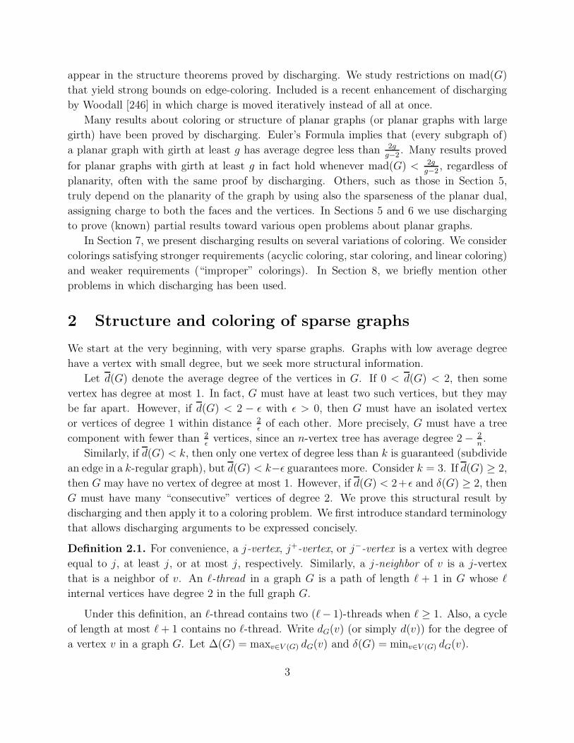
Definition 2.1. For convenience, a j-vertex, j+-vertex, or j−-vertex is a vertex with degree
equal to j, at least j, or at most j, respectively. Similarly, a j-neighbor of v is a j-vertex
that is a neighbor of v. An ℓ-thread in a graph G is a path of length ℓ + 1 in G whose ℓ
internal vertices have degree 2 in the full graph G.
Under this definition, an ℓ-thread contains two (ℓ− 1)-threads when ℓ ≥ 1. Also, a cycle
of length at most ℓ+ 1 contains no ℓ-thread. Write dG(v) (or simply d(v)) for the degree of
a vertex v in a graph G. Let ∆(G) = maxv∈V (G) dG(v) and δ(G) = minv∈V (G) dG(v).
3
Proposition 2.2. If d(G) < 2+ 13t−2
and G has no 2-regular component, then G contains a
1−-vertex or a (2t− 1)-thread.
Proof. Let ρ = 12
13t−2
. Give each vertex v its degree d(v) as initial charge. If neither
configuration occurs in G, then we redistribute charge to leave each vertex with charge at
least 2 + 2ρ. If G has no 1−-vertex, then δ(G) ≥ 2. We then redistribute charge as follows.
(R1) Each 2-vertex takes ρ from each end of the maximal thread containing it.
Each 2-vertex receives charge 2ρ and ends with 2 + 2ρ. With (2t− 1)-threads forbidden,
each 3+-vertex v loses at most d(v)(2t− 2)ρ. For a lower bound on its final charge, we find
d(v)− d(v)(2t− 2)ρ ≥ 3
[
1− t− 1
3t− 2
]
= 2 +1
3t− 2= 2 + 2ρ.
We have proved that forbidding the specified configurations requires d(G) ≥ 2 + 13t−2
.
The idea is simple; if no desired configuration occurs, then charge can be redistributed
to contradict the hypothesis. The details are also easily checked. The mystery is where the
discharging rule and the hypothesis on d(G) come from. The secret is that the discharging
rule is found before one even knows what the hypothesis on d(G) will be and is used to
discover that hypothesis.
Remark 2.3. For discharging proofs when d(G) < 2+2ρ, only 2-vertices need to gain charge
(after restricting to δ(G) ≥ 2), but we must ensure that 3+-vertices don’t lose too much.
The natural sources of charge for the 2-vertices are the nearest vertices of larger degree.
To select ρ, we seek the weakest hypothesis that avoids taking too much charge from
3+-vertices. With ℓ-threads forbidden, each 3+-vertex loses at most (ℓ − 1)ρ along each
incident thread. For a j-vertex, we thus need j − j(ℓ − 1)ρ ≥ 2 + 2ρ, which simplifies to
ρ ≤ j−2j(ℓ−1)+2
. With ℓ fixed (and j ≥ 3), the bound is tightest when j = 3. Therefore, setting
ρ = 13ℓ−1
makes the proof work and also gives the weakest hypothesis where it works. We
used ℓ = 2t − 1 in Proposition 2.2 for consistency with the intended application, but the
statement and argument are valid for all ℓ.
The structure theorem is sharp. From the proof, all vertices in a sharpness example
should have degree 2 or 3. To generate infinitely many such examples, replace each edge of
any 3-regular n-vertex graph with an (ℓ− 1)-thread. Long threads do not occur, and there
are ℓ3n2edges and n + (ℓ− 1)3n
2vertices; the average degree is 2 + 2
3ℓ−1.
Discovering a discharging argument is fun in itself, but the value is in applications. To
use structural results in inductive proofs, we must require the hypothesis of the structural
lemma to hold also in subgraphs.
A graph is d-degenerate if every subgraph has a vertex of degree at most d; this is an
“every subgraph” analogue of δ(G) ≤ d. A k-coloring of a graph G labels vertices using a
4
set of k colors; a coloring is proper if adjacent vertices always have distinct colors. A graph
is k-colorable if it has a proper k-coloring, and the chromatic number χ(G) is the least such
k. Every (k − 1)-degenerate graph is k-colorable, by induction on the number of vertices.
Using bounds on average degree analogously to obtain good colorings requires all sub-
graphs to satisfy the same bound. Hence we restrict the maximum average degree over all
subgraphs, denoted by mad(G). Note that mad(G) < k implies that G is (k−1)-degenerate.
Thus we already have χ(G) ≤ k when mad(G) < k. Even when mad(G) = k− 1, we cannot
improve the bound on χ(G), due to the complete graph Kk. Hence to obtain stronger color-
ing results when mad(G) < k, we consider a more refined notion of chromatic number. Let
Zp denote the set of congruence classes of integers modulo p; here p is any positive integer.
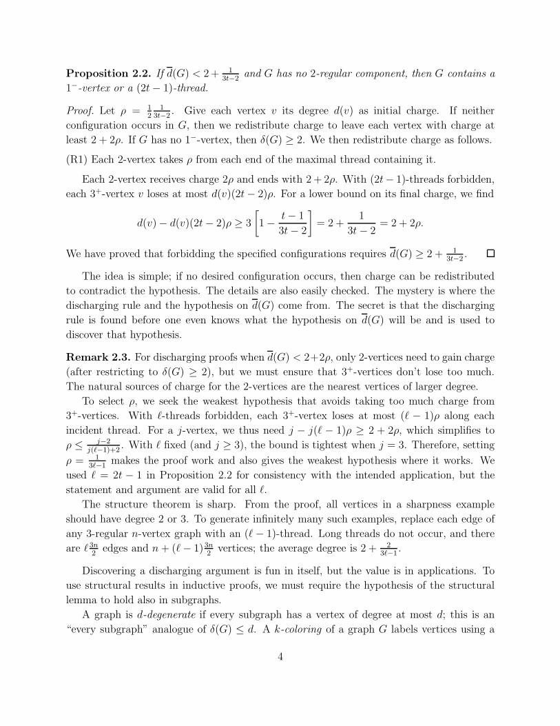
Definition 2.4. A homomorphism from a graph G to a graph H is a map φ : V (G) → V (H)
such that uv ∈ E(G) implies φ(u)φ(v) ∈ E(H). Such a map is an H-coloring ; the vertices
of G are “colored” by vertices of H . Let Kp:q be the graph with vertex set Zp in which
vertices are adjacent when they differ by at least q (see Figure 1). A (p, q)-coloring of G is
a homomorphism from G into Kp:q. A graph having a (p, q)-coloring is (p, q)-colorable. The
circular chromatic number of G, written χc(G), is infpq: G is (p, q)-colorable.
••
••
•
0
1
23
4• •
•••
••
01
2
34
5
6 • ••
•••••
01
2
34
5
6
7
Figure 1: K5:2, K7:3, and K8:3
The term “circular coloring” suggests viewing the colors as equally-spaced points on a
circle. A (p, q)-coloring φ then uses colors in 0, . . . , p− 1 so that q ≤ |φ(u)− φ(v)| ≤ p− q
when uv ∈ E(G). A (k, 1)-coloring is just a proper k-coloring. Zhu [258] surveyed basic facts
about circular coloring, which include that χc(G) is a well-defined rational number (“inf”
becomes “min”) and that ⌈χc(G)⌉ = χ(G). Thus χc(G) gives more information than χ(G).
Also, if G has a (p, q)-coloring and p′
q′≥ p
q, then G also has a (p′, q′)-coloring.
Note that K(2t+1):t is isomorphic to C2t+1. Thus χc(G) ≤ 2 + 1tif and only if there is a
homomorphism from G into C2t+1, which cannot happen if G has a shorter odd cycle. Let
go(G) denote the length of a shortest odd cycle in G, with go(G) = ∞ when G is bipartite.
Requiring go(G) ≥ 2t+ 1 gives us a chance to prove χc(G) ≤ 2 + 1t.
Proposition 2.5. Fix t ∈ N. If go(G) ≥ 2t+1 and mad(G) < 2+ 13t−2
, then χc(G) ≤ 2+ 1t.
Proof. If G = K1 or G is a cycle, then χc(G) ≤ 2 + 1t. With this as basis, we use induction
on |V (G)| to obtain a homomorphism from G into C2t+1. When G is neither K1 nor a
5
cycle, Proposition 2.2 implies that G has either a 1−-vertex or a (2t− 1)-thread. Note that
go(G′) ≥ 2t+ 1 and mad(G′) < 2 + 1
3t−2whenever G′ is an induced subgraph of G.
If G has a 1−-vertex u, then let φ be a homomorphism of G−u into C2t+1, as guaranteed
by the induction hypothesis. To extend φ to G, when u is isolated we can give it any color.
When u has a neighbor v, we can assign u either neighbor of φ(v) in C2t+1.
Otherwise, G contains a thread P with endpoints v and w that has internal vertices
u1, . . . , u2t−1. Let G′ = G − u1, . . . , u2t−1. Since mad(G′) < 2 + 13t−2
, the induction
hypothesis yields a homomorphism φ from G′ to C2t+1. To extend φ to the desired coloring
of G, map the internal vertices of P to the internal vertices of a walk of length 2t from φ(v)
to φ(w) in C2t+1. This extension exists because any two vertices of C2t+1 are joined by a
path of even length at most 2t. To follow a path of length 2s in 2t steps, repeat one edge
2t− 2s+ 1 times in succession.
We need a (2t − 1)-thread in the induction step because with shorter threads there are
choices for the colors at the endpoints that do not permit extension along the thread. For
example, if the endpoints of a (2t − 2)-thread have the same color, then a C2t+1-coloring
cannot be extended along the thread.
Note again that the structural lemma uses only a bound on d(G). Only the application
requires the bound also for all subgraphs. In any hereditary family G, a bound on d(G) that
holds for all G ∈ G immediately yields the same bound on mad(G).
The structural result in Proposition 2.2 is sharp, but Proposition 2.5 is not. We can
improve it by considering more configurations, with the same proof idea. Let the weak
2-neighbors of a vertex v be the 2-vertices lying on threads incident to v.
Lemma 2.6. If d(G) < 2 + 12t−1
and G has no 2-regular component, then G contains (1) a
1−-vertex, or (2) a 3-vertex with at least 4t−3 weak 2-neighbors, or (3) a 4+-vertex incident
to a (2t− 1)-thread.
Proof. Let ρ = 12
12t−1
. Assign each vertex v initial charge d(v). We may assume δ(G) ≥ 2.
Redistribute charge using the same rule as before.
(R1) Each 2-vertex takes ρ from each end of the maximal thread containing it.
As in Proposition 2.2, each 2-vertex finishes with 2 + 2ρ. If no 3-vertex has 4t− 3 weak
2-neighbors, then each 3-vertex v loses charge at most (4t − 4)ρ and hence retains at least
3− 2t−22t−1
, which equals 2 + 2ρ.
Now let v be a 4+-vertex. If v has no incident (2t− 1)-thread, then v gives charge to at
most 2t−2 vertices on each incident thread. The minimum remaining charge d(v)[1−(2t−2)ρ]
is minimized when d(v) = 4. We compute 4[1 − (2t− 2)ρ] = 4 − 22t−22t−1
= 2 + 4ρ. (There is
not enough excess charge to force a longer thread; fortunately, this is just long enough!)
Every vertex finishes with charge at least 2+ 2ρ, so avoiding the specified configurations
requires mad(G) ≥ 2 + 12t−1
.
6
This structural result is driven by the application, where a 3-vertex with 4t − 3 weak
2-neighbors is reducible. Balancing the needs of 2-vertices and 3-vertices then governs the
choice of ρ to make the result apply to the largest family. When the reducible configurations
at 1−-vertices and 3-vertices do not arise, some thread is long enough to be reducible.
Lemma 2.6 yields a better coloring bound than Proposition 2.5, because we now have a
more flexible way of extending circular colorings of subgraphs. We need a well-known lemma
about extension of circular colorings, illustrated in Figure 2
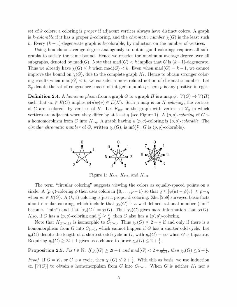
Lemma 2.7. Assume p > 2q, and let P be an ℓ-thread with endpoints x and y in a graph
G. In a (p, q)-coloring φ, a fixed choice of φ(x) can be extended along P with at most
max0, p− 1− (ℓ+ 1)(p− 2q) values in Zp forbidden as φ(y).
Proof. Let u0 = x and uℓ+1 = y, so P = 〈u0, u1, . . . , uℓ, uℓ+1〉. We claim that the colors
allowed at ui include 1 + i(p − 2q) consecutive colors in Zp, true by definition for i = 0. If
the colors from a through b (modulo p) are allowed at ui, then the colors from a+ q through
b+ (p− q) are allowed at ui+1. The size of the new interval exceeds the size of the previous
interval by p− 2q. When ℓ+ 1 ≥ p−1p−2q
, there is no restriction at y from this thread.
• • • • • • •
•
•(p, q) = (5, 2)
01
0
2,34,0,1
4
3,4 0,1,22,3
Figure 2: Extension of (5, 2)-coloring along three threads; allowed colors shown
We now adopt the language of “minimal counterexample” for inductive proofs. Most
applications of structure theorems proved by discharging are proved for hereditary graph
classes. Proving reducibility of forced configurations then completes an inductive proof,
since it forbids the existence of a minimal counterexample to the claim.
Theorem 2.8. If go(G) ≥ 2t+ 1 and mad(G) < 2 + 12t, then χc(G) ≤ 2 + 1
t.
Proof. Let G be a minimal graph satisfying the hypotheses but not the conclusion; the
hypotheses hold for all subgraphs of G. The claim holds for cycles, so we may forbid 2-regular
components. Lemma 2.6 then guarantees one of three configurations in G. We already
showed in Theorem 2.5 that 1−-vertices and (2t−1)-threads are reducible for χc(G) ≤ 2+ 1t.
It remains only to show that a minimal counterexample cannot contain a 3-vertex v with
at least 4t − 3 weak 2-neighbors. If G is such a graph, then form G′ from G by deleting v
and all its weak 2-neighbors. Extending a C2t+1-coloring of G′ along the threads incident to
v completes a C2t+1-coloring of G if some color in Z2t+1 is not forbidden at v.
7
Let li be the number of 2-vertices along the ith thread at v. By Lemma 2.7 with p = 2t+1
and q = t, this thread forbids at most (2t) − (li + 1)1 colors from use at v. Together, the
three threads forbid at most (6t)− (l1 + l2 + l3 + 3) colors. Since∑
li ≥ 4t− 3, at most 2t
colors are forbidden, so some color remains available for a simultaneous extension along the
three threads to complete a C2t+1-coloring of G.
To see that Theorem 2.8 improves Proposition 2.5, note that the conclusion (G is (2+ 1t)-
colorable) is the same in both, but the hypothesis on mad(G) is weaker in Theorem 2.8
(mad(G) < 2 + 12t) than in Proposition 2.5 (mad(G) < 2 + 1
3t−2). Weakening the hypoth-
esis introduces graphs avoiding the unavoidable set in Proposition 2.2, but then another
configuration is forced that is also reducible for the desired conclusion.
The bound on mad(G) in Theorem 2.8 is still not sharp for χc(G) ≤ 2+ 1t. In particular,
Borodin et al. [52] proved for triangle-free graphs that mad(G) < 125
implies χc(G) ≤ 52,
while Theorem 2.8 with t = 2 requires mad(G) < 94to obtain χc(G) ≤ 5
2. Sharpness of their
result follows from the case t = 2 of the following construction.
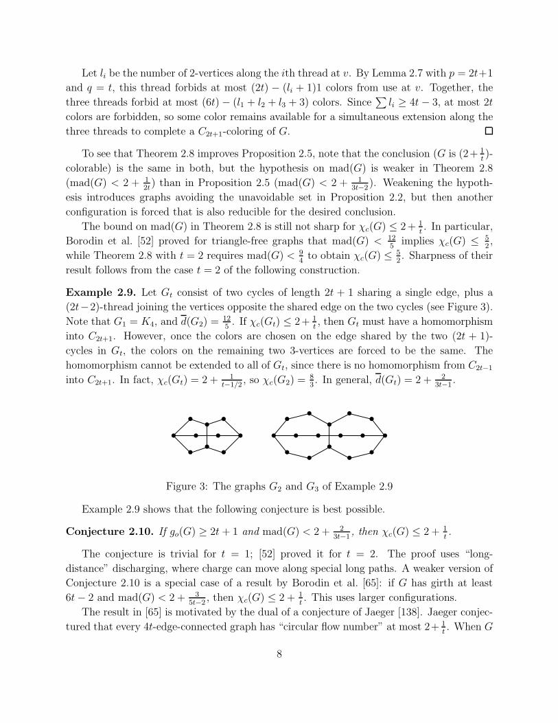
Example 2.9. Let Gt consist of two cycles of length 2t + 1 sharing a single edge, plus a
(2t−2)-thread joining the vertices opposite the shared edge on the two cycles (see Figure 3).
Note that G1 = K4, and d(G2) =125. If χc(Gt) ≤ 2+ 1
t, then Gt must have a homomorphism
into C2t+1. However, once the colors are chosen on the edge shared by the two (2t + 1)-
cycles in Gt, the colors on the remaining two 3-vertices are forced to be the same. The
homomorphism cannot be extended to all of Gt, since there is no homomorphism from C2t−1
into C2t+1. In fact, χc(Gt) = 2 + 1t−1/2
, so χc(G2) =83. In general, d(Gt) = 2 + 2
3t−1.
• • • ••
••
•
•
•• • • • • •
•
•• •
• •
••
••
Figure 3: The graphs G2 and G3 of Example 2.9
Example 2.9 shows that the following conjecture is best possible.
Conjecture 2.10. If go(G) ≥ 2t + 1 and mad(G) < 2 + 23t−1
, then χc(G) ≤ 2 + 1t.
The conjecture is trivial for t = 1; [52] proved it for t = 2. The proof uses “long-
distance” discharging, where charge can move along special long paths. A weaker version of
Conjecture 2.10 is a special case of a result by Borodin et al. [65]: if G has girth at least
6t− 2 and mad(G) < 2 + 35t−2
, then χc(G) ≤ 2 + 1t. This uses larger configurations.
The result in [65] is motivated by the dual of a conjecture of Jaeger [138]. Jaeger conjec-
tured that every 4t-edge-connected graph has “circular flow number” at most 2+ 1t. When G
8
is planar, making this statement for the dual graph G∗ yields χc(G) ≤ 2+ 1twhen G has girth
at least 4t. Lovasz, Thomassen, Wu, and Zhang [173] proved the weaker form of Jaeger’s
Conjecture replacing 4t by 6t. Thus χc(G) ≤ 2 + 1twhen G is planar with girth at least 6t.
By Euler’s Formula, mad(G) < 2gg−2
when G is planar with girth g. Thus mad(G) < 2+ 22t−1
when G is planar with girth at least 4t. Conjecture 2.10 in some sense proposes a trade-
off: by further restricting to mad(G) < 2 + 23t−1
, the girth requirement can be relaxed to
go(G) ≥ 2t+ 1 and still yield χc(G) ≤ 2 + 1t, even without requiring planarity.
We have discussed only very sparse graphs and very small χc(G), but the problem can be
studied in general. Always χ(G) ≥ ω(G), where ω(G) is the maximum number of pairwise
adjacent vertices in G, called the clique number of G. The circular clique number, written
ωc(G), is maxpq: Kp:q ⊆ G; note that χc(G) ≥ ωc(G).
Problem 2.11. Among graphs G with ωc(G) ≤ s, what is the largest ρ such that mad(G) <
ρ implies χc(G) ≤ s?
The answer ρ satisfies ⌊s⌋ ≤ ρ < s. The question generalizes the statement that (k− 1)-
degenerate graphs are k-colorable but Kk+1 is not. If mad(G) < ⌊s⌋, then G is ⌊s⌋-colorableand hence also s-colorable. If mad(G) = s, then G may be Kp:q with p
q= s. Problem 2.11
has not been studied much, but discharging should permit some progress on it.
Exercise 2.1. Let G be a graph with δ(G) = 2 and mad(G) < 3. Prove that G has a 2-vertex witha 5−-neighbor. Prove that this is sharp in the sense that the conclusion may fail when mad(G) = 3.
Exercise 2.2. Given 0 ≤ j < k, let G be a graph with δ(G) = k. Determine the largest ρ suchthat d(G) < k + ρ guarantees that G has a k-vertex having more than j neighbors of degree k.
Exercise 2.3. Show that Lemma 2.6 is sharp. For each t ∈ N construct infinitely many exampleswith average degree 2 + 1
2t−1 in which none of the specified configurations occurs.
Exercise 2.4. (Cranston–Kim–Yu [93]) Let G be a connected graph with at least four vertices.Prove that if d(G) < 5
2 and δ(G) ≥ 2, then G contains a 2-thread or a 3-vertex having three2-neighbors, one of which has a second 3-neighbor.
Exercise 2.5. (Cranston–Jahanbekam–West [91]) Prove that if d(G) < 52 and G is connected,
then G contains a 3−-vertex with a 1-neighbor, a 4−-vertex with two 2−-neighbors, or a 5+-vertex v with at least d(v)−1
2 2−-neighbors. (Comment: These configurations are reducible forthe “1, 2-Conjecture” of Przyby lo and Wozniak [190]. Although that proves the conjecture whenmad(G) < 5
2 , [190] proved the stronger result that the conjecture holds for 3-colorable graphs.)
Exercise 2.6. Prove that if mad(G) < k + ρ with 0 < ρ ≤ kk+1 , then G contains a (k− 1)−-vertex,
two adjacent k-vertices, or a (k + 1)-vertex with more than (1ρ − 1)k neighbors having degree k.
Construct sharpness examples with mad(G) = k + ρ when ρ = 12 and when ρ = k
k+1 (the lattermay have maximum degree k + 1 or k + 2).
Exercise 2.7. Prove that if ∆(G) = k ≥ 3 and mad(G) < k − 2k2+1
, then G contains one of the
following configurations: (C1) a (k−2)−-vertex, (C2) two adjacent (k−1)-vertices, (C3) a k-vertexwith two (k− 1)-neighbors, (C4) two adjacent k-vertices each having a (k− 1)-neighbor, or (C5) ak-vertex having three k-neighbors such that each is adjacent to a (k − 1)-vertex.
9
3 List Coloring
Reducibility arguments for coloring often involve deleting some parts of a graph and then
choosing colors for the missing pieces as they are reinserted. Suitable choices can be made
if there are enough available colors; it does not really matter what the colors are. In this
situation, the arguments often extend to yield stronger results about coloring from lists.
Definition 3.1. A list assignment on a graph G is a map L giving each v ∈ V (G) a set
L(v) of colors called its list. In a k-uniform list assignment, each list has size k. Given a list
assignment L on G, an L-coloring of G is a proper coloring φ of G such that φ(v) ∈ L(v)
for all v ∈ V (G). A graph G is k-choosable if G is L-colorable whenever each list has size at
least k (we may assume L is k-uniform). The list chromatic number of G, written χℓ(G), is
the least k such that G is k-choosable.
Since the lists could be identical, always χℓ(G) ≥ χ(G). Thus proving χℓ(G) ≤ b strength-
ens a result that χ(G) ≤ b. For example, Brooks’ Theorem states that χ(G) ≤ ∆(G) when
G is a connected graph that is not a complete graph or an odd cycle; Erdos, Rubin, and
Taylor [105] proved the same bound for χℓ(G). Although χℓ(G) may be larger for 2-colorable
graphs (Exercise 3.1), cycles of even length are well behaved; we will need this fact.
Lemma 3.2. Even cycles are 2-choosable.
Proof. We show that C2t is L-colorable when every list has size 2. If the lists are identical,
then choose the colors to alternate. Otherwise, there are adjacent vertices x and y such that
L(x) contains a color c not in L(y). Use c on x, and then follow the path C2t − x from x to
y to color the vertices other than x: at each new vertex, choose a color from its list that was
not chosen for the previous vertex. Such a choice is always available, and they satisfy every
edge because the colors chosen on x and y differ.
Coloring and list-coloring have been studied extensively for squares of graphs. Given a
graph G, let G2 be the graph obtained from G by adding edges to join vertices that are
distance 2 apart in G. The neighbors of a vertex v in G form a clique with v in G2, so always
χ(G2) ≥ ∆(G) + 1. Kostochka and Woodall [158] conjectured that always χℓ(G2) = χ(G2).
This was proved in special cases, but Kim and Park [149] disproved it in general. They used
orthogonal families of Latin squares to construct a graph G for prime p such that G2 is the
complete (2p− 1)-partite graph Kp,...,p; on such graphs, χℓ − χ is unbounded.
Thus sufficient conditions for χℓ(G2) = ∆(G)+1 hold only on special classes but establish
a strong property. We present such a result to show how a discharging proof is discovered.
The Discharging Method often begins with configurations that are easy to show reducible. A
discharging proof of unavoidability of a set of such configurations starts by forbidding them.
When discharging, we may encounter a situation that does not guarantee the desired final
10
charge on some vertices. Instead of trying to adjust the discharging rules, we may try to
add this configuration to the unavoidable set, allowing us to assume that it does not occur.
This approach succeeds if we can show that the new configuration is reducible.
We use NG(v) for the neighborhood of a vertex v in a graph G, with NG[v] = NG(v)∪v.
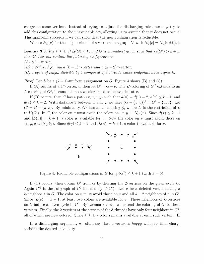
Lemma 3.3. Fix k ≥ 4. If ∆(G) ≤ k, and G is a smallest graph such that χℓ(G2) > k + 1,
then G does not contain the following configurations:
(A) a 1−-vertex,
(B) a 2-thread joining a (k − 1)−-vertex and a (k − 2)−-vertex,
(C) a cycle of length divisible by 4 composed of 3-threads whose endpoints have degree k.
Proof. Let L be a (k + 1)-uniform assignment on G; Figure 4 shows (B) and (C).
If (A) occurs at a 1−-vertex v, then let G′ = G− v. The L′-coloring of G′2 extends to an
L-coloring of G2, because at most k colors need to be avoided at v.
If (B) occurs, then G has a path 〈x, u, v, y〉 such that d(u) = d(v) = 2, d(x) ≤ k− 1, and
d(y) ≤ k − 2. With distance 3 between x and y, we have (G − u, v)2 = G2 − u, v. Let
G′ = G − u, v. By minimality, G′2 has an L′-coloring φ, where L′ is the restriction of L
to V (G′). In G, the color on u must avoid the colors on x, y ∪NG′(x). Since d(x) ≤ k− 1
and |L(u)| = k + 1, a color is available for u. Now the color on v must avoid those on
x, y, u ∪NG′(y). Since d(y) ≤ k − 2 and |L(u)| = k + 1, a color is available for v.
• • • • ••••
•••• • • • •
v zv′z′
• • • •x u v y
B
C
Figure 4: Reducible configurations in G for χℓ(G2) ≤ k + 1 (with k = 5)
If (C) occurs, then obtain G′ from G by deleting the 2-vertices on the given cycle C.
Again G′2 is the subgraph of G2 induced by V (G′). Let v be a deleted vertex having a
k-neighbor z in G. The color on v must avoid those on z and all k − 2 neighbors of z in G′.
Since |L(v)| = k + 1, at least two colors are available for v. These neighbors of k-vertices
on C induce an even cycle in G2. By Lemma 3.2, we can extend the coloring of G′ to these
vertices. Finally, the 2-vertices at the centers of the 3-threads have only four neighbors in G2,
all of which are now colored. Since k ≥ 4, a color remains available at each such vertex.
In a discharging argument, we often say that a vertex is happy when its final charge
satisfies the desired inequality.
11
Theorem 3.4 ([35, 95]). If ∆(G) ≤ 6 and mad(G) < 52, then χℓ(G
2) = 7.
Proof. Let G be a minimal counterexample. Let k = 6. By Lemma 3.3(A), we may assume
δ(G) ≥ 2. By Lemma 3.3(B), G has no 4-thread (or longer), and 3-threads have k-vertices
at both ends. By Lemma 3.3(C), the union of the 3-threads is an acyclic subgraph H .
Let each leaf of H sponsor its incident 3-thread, delete the edges of the sponsored 3-
threads, and repeat. When a component of what remains has just one 3-thread, pick one
endpoint as the sponsor. In this way, each 3-thread in G receives one of its endpoints as a
sponsoring k-vertex, and each k-vertex is chosen at most once as a sponsor.
We now seek discharging rules to prove that if mad(G) < 52and δ(G) ≥ 2, then some
configuration of type (B) or (C) in Lemma 3.3 must occur. This will not quite work; we will
need to add more configurations to the set, but they will be reducible. A vertex is high if its
degree is 5 or 6; medium if it is 3 or 4. Each vertex v has initial charge d(v); we seek final
charge at least 52. We treat the internal vertices of a j-thread together; they need to receive
at least j2. Here by “j-thread” we refer only to j-threads whose endpoints are 3+-vertices.
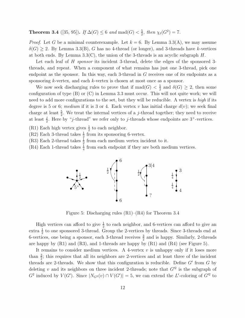
(R1) Each high vertex gives 12to each neighbor.
(R2) Each 3-thread takes 12from its sponsoring 6-vertex.
(R3) Each 2-thread takes 12from each medium vertex incident to it.
(R4) Each 1-thread takes 14from each endpoint if they are both medium vertices.
•
••
••
•
5+
12
•
•
•
•
•
6
6
12
•
•
•
•
?
3|412
•
•
•
4
314
14
Figure 5: Discharging rules (R1)–(R4) for Theorem 3.4
High vertices can afford to give 12to each neighbor, and 6-vertices can afford to give an
extra 12to one sponsored 3-thread. Group the 2-vertices by threads. Since 3-threads end at
6-vertices, one being a sponsor, each 3-thread receives 32and is happy. Similarly, 2-threads
are happy by (R1) and (R3), and 1-threads are happy by (R1) and (R4) (see Figure 5).
It remains to consider medium vertices. A 4-vertex v is unhappy only if it loses more
than 32; this requires that all its neighbors are 2-vertices and at least three of the incident
threads are 2-threads. We show that this configuration is reducible. Define G′ from G by
deleting v and its neighbors on three incident 2-threads; note that G′2 is the subgraph of
G2 induced by V (G′). Since |NG2(v) ∩ V (G′)| = 5, we can extend the L′-coloring of G′2 to
12
v. When we restore the deleted 2-neighbors of v, the numbers of vertices whose colors they
must avoid are 4, 5, 6, respectively, so at each step a color is available.
Since it gives at most 12to each thread, an unhappy 3-vertex v has no high neighbor and
loses more than 12. It may give charge at least 1
4to each of three threads or give 1
2to one
thread and at least 14to another.
In the first case, let NG(v) = x1, x2, x3, and let G′ = G − NG[v]. The neighbor of xi
other than v has degree at most 4. As we restore NG(v), the number of vertices whose colors
they must avoid are 4, 5, 6, so at each step a color is available. We can then replace v; it
must avoid the colors on six vertices.
In the second case, v has two 2-neighbors. Let z be the medium neighbor of v, let x be
the neighbor on a thread receiving 12from v (it is a 2-thread), and let y be the remaining
neighbor (y is a 2-vertex whose other neighbor is a 4−-vertex). With S = v, x, y, letG′ = G− S; again G′2 = G2 − S. Restore v, then y, then x. As each is restored, its color is
chosen from its list to avoid the colors on at most six other vertices.
Cranston and Skrekovski [95] proved more generally that if ∆(G) ≥ 6 and mad(G) <
2 + 4∆(G)−85∆(G)+2
, then χℓ(G2) = ∆(G) + 1. Thus when mad(G) is sufficiently small compared to
∆(G), the trivial lower bounds on χ(G2) and χℓ(G2) are tight. With a similar but shorter
proof, Bonamy, Leveque, and Pinlou [35] proved the less precise statement that for each
positive ǫ, there exists kǫ such that χℓ(G2) = ∆(G)+1 for ∆(G) ≥ kǫ when mad(G) < 14
5−ǫ.
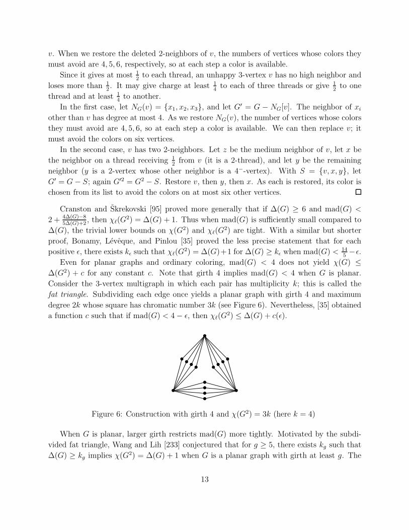
Even for planar graphs and ordinary coloring, mad(G) < 4 does not yield χ(G) ≤∆(G2) + c for any constant c. Note that girth 4 implies mad(G) < 4 when G is planar.
Consider the 3-vertex multigraph in which each pair has multiplicity k; this is called the
fat triangle. Subdividing each edge once yields a planar graph with girth 4 and maximum
degree 2k whose square has chromatic number 3k (see Figure 6). Nevertheless, [35] obtained
a function c such that if mad(G) < 4− ǫ, then χℓ(G2) ≤ ∆(G) + c(ǫ).
•
••
••••
••••
••••
Figure 6: Construction with girth 4 and χ(G2) = 3k (here k = 4)
When G is planar, larger girth restricts mad(G) more tightly. Motivated by the subdi-
vided fat triangle, Wang and Lih [233] conjectured that for g ≥ 5, there exists kg such that
∆(G) ≥ kg implies χ(G2) = ∆(G) + 1 when G is a planar graph with girth at least g. The
13
conjecture is false for g ∈ 5, 6; [50] and [100] both contain infinite sequences of planar
graphs with girth 6, growing maximum degree, and χ(G2) = ∆(G) + 2.
However, the Wang–Lih Conjecture holds and can be strengthened to list coloring when
g ≥ 7. Ivanova [137] proved χℓ(G2) = ∆(G) + 1 for planar G having girth at least 7 and
∆(G) ≥ 16 (improving on ∆(G) ≥ 30 from [50]), and she also showed that the thresholds
10, 6, 5 on ∆(G) are sufficient when G has girth at least 8, 10, 12, respectively.
For girth 6, Dvorak, Kral’, Nejedly, and Skrekovski [100] proved χ(G2) ≤ ∆(G) + 2 for
planar G with ∆(G) ≥ 8821 (they also conjectured χ(G2) ≤ ∆(G) + 2 for girth 5 when
∆(G) is large enough). For girth 6, Borodin and Ivanova [54] improved ∆(G) ≥ 8821 to
∆(G) ≥ 18; they also showed that ∆(G) ≥ 24 yields χℓ(G2) ≤ ∆(G) + 2 [55].
Bonamy, Leveque, and Pinlou [34] proved χℓ(G2) ≤ ∆(G) + 2 when ∆(G) ≥ 17 and
mad(G) < 3, regardless of planarity. As we have noted, mad(G) < 2gg−2
when G is a planar
graph with girth at least g, so the result of [34] is stronger than saying that χℓ(G2) ≤ ∆(G)+2
for all planar graphs with girth at least 6 and maximum degree at least 17.
Now consider again the result of Cranston and Skrekovski [95]. Reducing the bound on
mad(G) from 3 to 2 + 4∆(G)−85∆(G)+2
yields χℓ(G2) = ∆(G) + 1 rather than χℓ(G
2) ≤ ∆(G) + 2,
even for the larger family where ∆(G) ≥ 6. Furthermore, as ∆(G) grows, the needed bound
on mad(G) tends to 145, which is the bound guaranteed for planar graphs with girth at least
7. Hence it seems plausible that χℓ(G2) = ∆(G) + 1 for planar graphs with girth at least 7
even when ∆(G) ≥ 6. For fuller understanding of this parameter, we suggest a problem.
Problem 3.5. Among the family of graphs such that ∆(G) ≥ k, what is the largest value
bj,k such that mad(G) < bj,k implies χℓ(G2) ≤ ∆(G) + j?
Next we weaken the requirements. A coloring where vertices at distance 2 have distinct
colors but adjacent vertices need not is an injective coloring (the coloring is injective on
each vertex neighborhood). The injective chromatic number, written χi(G), is the minimum
number of colors needed, and the injective choice number, χiℓ(G), is the least k such that G
has an injective L-coloring when L is any k-uniform list assignment.
From the definition, always χi(G) ≤ χ(G2) and χiℓ(G) ≤ χℓ(G
2). The trivial lower bound
on χi(G) is ∆(G) rather than ∆(G) + 1. We seek results like those above, with a bound on
χi(G) or χiℓ(G) that is one less than the corresponding bound for χ(G2) or χℓ(G
2). Again
when mad(G) is small relative to ∆(G), the value is close to the lower bound. In [34], for
example, it is noted that the proof there also yields χiℓ(G) ≤ ∆(G)+ 1 when ∆(G) ≥ 17 and
mad(G) < 3. Similarly, the proof in [95] yields χiℓ(G) = ∆(G) under the conditions there.
Nevertheless, the analogue of Problem 3.5 for injective coloring remains largely open.
When j = 0, rather tight bounds on mad(G) suffice. Cranston, Kim, and Yu [93] proved
that χi(G) = ∆(G) when mad(G) < 4219
and ∆(G) ≥ 3. Sharpness is not known, even for
∆(G) = 3. Subdividing one edge of K4 yields a graph H such that χ′(H) > ∆(H), and
then subdividing every edge of H yields a bipartite graph G such that χi(G) > ∆(G) and
14

mad(G) = 73. The largest b such that mad(G) < b implies χi(G) = ∆(G) when ∆(G) = 3 is
not known; it is at least 4219
and at most 73.
To yield χiℓ(G) ≤ ∆(G) + 1, it suffices to have mad(G) ≤ 5
2when ∆(G) ≥ 3 [93]. For
∆(G) ≥ 4 this is fairly easy (it uses Exercise 2.4); for ∆(G) ≥ 6 it follows from [95].
To yield χiℓ(G) ≤ ∆(G) + 2, it suffices to have mad(G) < 36
13when ∆(G) = 3 [94]; we
will see that this is sharp. For ∆(G) ≥ 4, it suffices to have mad(G) < 145
[94]; the cases
∆(G) ∈ 4, 5 are difficult, and sharpness is not known. Note that when ∆(G) ≥ 4 the
allowed values of mad(G) are larger than when ∆(G) = 3; the loosest condition on mad(G)
that suffices for a given bound on χi(G)−∆(G) should grow (somewhat) as ∆(G) grows.
We use one of these results to further explore how discharging arguments are found. In
the discharging process, charge may travel distance 2.
Theorem 3.6. ([94]) If ∆(G) ≤ 3 and mad(G) < 3613, then χi
ℓ(G) ≤ 5.
Proof. We present the discharging argument and leave the reducibility of the configurations
in the resulting unavoidable set to Exercise 3.8. We claim that every graph G with ∆(G) = 3
and d(G) < 3613
contains one of the following configurations: a 1−-vertex, adjacent 2-vertices,
a 3-vertex with two 2-neighbors, or adjacent 3-vertices each having a 2-neighbor.
If none of these configurations occurs, then δ(G) ≥ 2. With initial charge equal to degree,
only 2-vertices need charge; all other vertices are 3-vertices. A way to allow 2-vertices to
reach charge 3613
without taking too much from 3-vertices is as follows:
(R1) Every 2-vertex takes 313
from each neighbor.
(R2) Every 2-vertex takes 113
via each path of length 2 from a 3-vertex.
Each 3-vertex v having a 2-neighbor gives it 313. Since no two 2-vertices are adjacent, and
adjacent 3-vertices cannot both have 2-neighbors, v loses no other charge. Each 3-vertex w
having no 2-neighbor loses at most 113
along each incident edge, because its 3-neighbors do
not have two 2-neighbors. (Under (R2), a 3-vertex opposite a 2-vertex x on a 4-cycle gives213
to x.) Thus every 3-vertex ends with charge at least 3613.
A 2-vertex gains 313
from each neighbor, and it also gains 113
along each of the two other
edges incident to each neighbor (see Figure 7). Hence it gains 1013
and reaches charge 3613.
(With no adjacent 3-vertices having 2-neighbors, no 2-vertex lies on a triangle.)
We have shown that d(G) ≥ 3613
when the specified configurations do not occur.
••
•
• •
•
• •
•
•
Figure 7: Discharging rules for Theorem 3.6; dashes move 113
15
Remark 3.7. The proof of Theorem 3.6 allows every vertex to end with charge exactly 3613.
This can happen, making the structure theorem sharp. In fact, here also the coloring result
is sharp. Deleting one vertex from the Heawood graph (the incidence graph of the Fano
plane) yields a graph H with d(H) = 3613, ∆(H) = 3, and χi(G) = 6.
The discharging rules in Theorem 3.6 follow naturally from the bound on mad(G) and the
forbidden configurations, but how are those found? To discover the structure theorem, first
study the coloring problem to find reducible configurations. A 1−-vertex and two adjacent
2-vertices are easy to show reducible. With a bit more thought, a 3-vertex with two 2-
neighbors is reducible. These configurations form an unavoidable set for mad(G) < 83, using
the discharging rule that each 2-vertex takes 13from each neighbor. That yields the desired
conclusion when mad(G) < 83, but we can do better.
After adding the reducible configuration consisting of two adjacent 3-vertices having 2-
neighbors, we seek the loosest bound on mad(G) under which this larger set is unavoidable.
It will exceed 83. The 2-vertices can take charge only from 3-vertices, but when mad(G) > 8
3
their neighbors cannot afford to give enough to satisfy them. When two adjacent 3-vertices
with 2-neighbors are forbidden, the 2-vertices can also gain charge along paths of length 2.
Now we have the “avenues” of discharging. Let each 2-vertex take a from each neighbor
and b along each path of length 2. Now 2-vertices end with 2 + 2a + 4b, 3-vertices having
2-neighbors end with 3 − a, and 3-vertices without 2-neighbors end with as little as 3− 3b.
We seek a and b to maximize the minimum of 2+2a+4b, 3− a, 3− 3b. If 3− a and 3− 3b
are not equal, then the value can be improved, so take a = 3b. Now min2 + 10b, 3− 3b is
maximized when 2+ 10b = 3− 3b, or b = 113. Hence the proof works when mad(G) < 36
13and
fails for any larger bound (as also implied by the sharpness example.).
Exercise 3.1. (Erdos–Rubin–Taylor [105], Vizing [228]) Prove that the complete bipartite graphKm,m is not k-choosable when m ≥
(2k−1k
)
. Determine the values of r such that Kk,r is k-choosable.
Exercise 3.2. (Cranston–Kim [92]) Apply Exercise 2.7 to prove that if ∆(G) ≤ 3 and mad(G) ≤ 145 ,
then χℓ(G2) ≤ 7.
Exercise 3.3. (Kim–Park [150]) Prove that if δ(G) ≥ 2 and d(G) < 4kk+2 with k ≥ 4, then G has
a 3−-vertex with a (k − 1)−-neighbor. Guarantee a 2-vertex with a (k − 1)−-neighbor when k ≤ 6.Conclude that if mad(G) < 4k
k+2 with k ≥ 4 (and no components are 5-cycles if k = 4), then fromany lists of size at least k a proper coloring of G can be chosen so that every vertex with degreeat least 2 has neighbors with distinct colors. Show also that this is sharp: there exists G withmad(G) = 4k
k+2 and an assignment of k-lists from which no such coloring can be chosen.
Exercise 3.4. In Problem 3.5, prove that b1,k ≥ 2. Show that equality holds when k ∈ 2, 3.
Exercise 3.5. (Cranston–Erman–Skrekovski [90]) Prove that a cycle of length divisible by 3 withvertices whose degrees cycle repeatedly through 2, 2, 3 is reducible for 5-choosability of G2. Usedischarging to conclude that if ∆(G) ≤ 4 and mad(G) < 16/7. then χℓ(G
2) ≤ 5.
16
Exercise 3.6. (Cranston–Erman–Skrekovski [90]) Prove that if ∆(G) ≤ 4 and d(G) < 187 , then
G contains one of: (C1) a 1−-vertex, (C2) two adjacent 2-vertices, (C3) a 3-vertex with three 2-neighbors, or (C4) a four-vertex path alternating between 2-vertices and 3-vertices. Conclude thatif ∆(G) ≤ 4 and mad(G) < 18
7 , then χℓ(G2) ≤ 7.
Exercise 3.7. (Cranston–Erman–Skrekovski [90]) Prove that if ∆(G) ≤ 4 and d(G) ≤ 103 , then G
contains one of: (C1) a 1−-vertex, (C2) a 2-vertex with a 3−-neighbor, (C3) a 3-vertex with two3-neighbors, or (C4) a 4-vertex with a 2-neighbor and a 3−-neighbor. Construct infinitely manygraphs with average degree 10
3 and maximum degree 4 that contain no such configuration. Provethat if ∆(G) ≤ 4 and mad(G) < 10
3 , then χl(G2) ≤ 12.
Exercise 3.8. (Cranston–Kim–Yu [94]) Complete the proof of Theorem 3.6 by showing that thoseconfigurations are reducible for χi(G) ≤ 5 in the family of graphs with ∆(G) ≤ 3.
Exercise 3.9. (Cranston–Kim–Yu [94]) Prove that if d(G) < 145 and ∆(G) ≥ 6, then G contains
one of the following configurations: (C1) a 1−-vertex, (C2) adjacent 2-vertices, (C3) a 3-vertex withneighbors of degrees 2, a, b, where a + b ≤ ∆(G) + 2, or (C4) a 4-vertex having four 2-neighbors,one of which has other neighbor of degree less than ∆(G). Argue that none of these configurationscan appear in a minimal graph G such that ∆(G) ≥ 6 and χi(G) > ∆(G) + 2. Reducibility of thefirst two configurations and part of (C3) is already requested in Exercise 3.8.
4 Edge-coloring and List Edge-coloring
A proper edge-coloring assigns colors to the edges of a graph G so that incident edges receive
distinct colors. The edge-chromatic number, written χ′(G), is the minimum number of colors
in such a coloring. Since the colors on edges with a common endpoint must be distinct,
always χ′(G) ≥ ∆(G). Vizing [224, 226] and Gupta [126] proved one of the most famous
theorems in graph coloring. It gives an upper bound for χ′(G) when G is a multigraph
(allowing multiedges) and specializes to the following for graphs (no loops or multiedges).
Theorem 4.1 (Vizing’s Theorem). If G is a graph, then ∆(G) ≤ χ′(G) ≤ ∆(G) + 1.
Recognition of χ′(G) = ∆(G) is NP-complete, so we seek sufficient conditions for equality.
Conjecture 4.2 (Vizing’s Planar Graph Conjecture [225, 227]). If G is a planar graph and
∆(G) ≥ 6, then χ′(G) = ∆(G).
Both conditions in Vizing’s Conjecture are needed. The complete graph K7 is 6-regular
but not planar. Each color can be used on at most three edges, so χ′(K7) ≥ 213= 7. Similarly,
obtain G from a 5-regular planar graph with 2k vertices by subdividing one edge. Since G
has 5k+ 1 edges, and at most k edges can receive the same color, χ′(G) ≥ 6. This difficulty
does not arise for ∆(G) ≥ 6, because regular planar graphs have degree at most 5.
Vizing [225] proved Conjecture 4.2 for ∆(G) ≥ 8, using Vizing’s Adjacency Lemma
(VAL). It is common to say that G is Class 1 if χ′(G) = ∆(G), Class 2 otherwise. An
17
edge-critical graph G is then a Class 2 graph such that χ′(G− e) = ∆(G) for all e ∈ E(G).
In fact, VAL implies that every edge-critical graph has at least three vertices of maximum
degree, so ∆(G) = ∆(G − e). Note also that every Class 2 graph contains an edge-critical
graph with the same maximum degree.
Theorem 4.3 (Vizing’s Adjacency Lemma [225]). If x and y are adjacent in an edge-critical
graph G, then at least max1 + ∆(G)− d(y), 2 neighbors of x have degree ∆(G).
Using VAL, Vizing proved the conjecture for ∆(G) ≥ 8 via counting arguments about
vertices of various degrees. The proof is clearer in the language of discharging, which was
not then in use. Luo and Zhang [174] used VAL and discharging to prove χ′(G) = ∆(G) for
the larger family of graphs G with mad(G) ≤ 6 and ∆(G) ≥ 8. We present a slightly simpler
proof of a slightly weaker result, requiring mad(G) < 6. In fact, Miao and Sun [175] proved
χ′(G) = ∆(G) also when ∆(G) ≥ 8 and mad(G) < 132. Their result (and that of [174]) uses
additional adjacency lemmas. Here VAL takes the place of reducibility arguments.
Theorem 4.4 ([174]). If G is a graph with mad(G) < 6 and ∆(G) ≥ 8, then χ′(G) = ∆(G).
Proof. Let G be a minimal counterexample, and let k = ∆(G). Since χ′(G) > k requires
an edge-critical subgraph with the same maximum degree, we may assume that G is edge-
critical. Since VAL gives each vertex at least two k-neighbors, δ(G) ≥ 2. We use discharging
with initial charge d(v); it suffices to show that each vertex ends with charge at least 6.
(R1) If d(v) ≤ 4, then v takes 6−d(v)d(v)
from each neighbor.
(R2) If d(v) ∈ 5, 6, then v takes 14from each 6+-neighbor.
For v ∈ V (G), let j be the least degree among vertices in NG(v). If j < k, then v has
at least k + 1 − j neighbors of degree k, by VAL. Hence k + 1 − j ≤ d(v)− 1, which yields
j ≥ 10− d(v) since k ≥ 8. Note that 7+-vertices take no charge.
If d(v) ≤ 4, then j ≥ 6, so v loses no charge, and (R1) sends enough to make v happy.
If d(v) = 5, then j ≥ 5. Furthermore, j = 5 yields k − 4 neighbors with degree k. Since
k ≥ 8, charge at least 4(14) comes to v, no charge is given away, and v is happy.
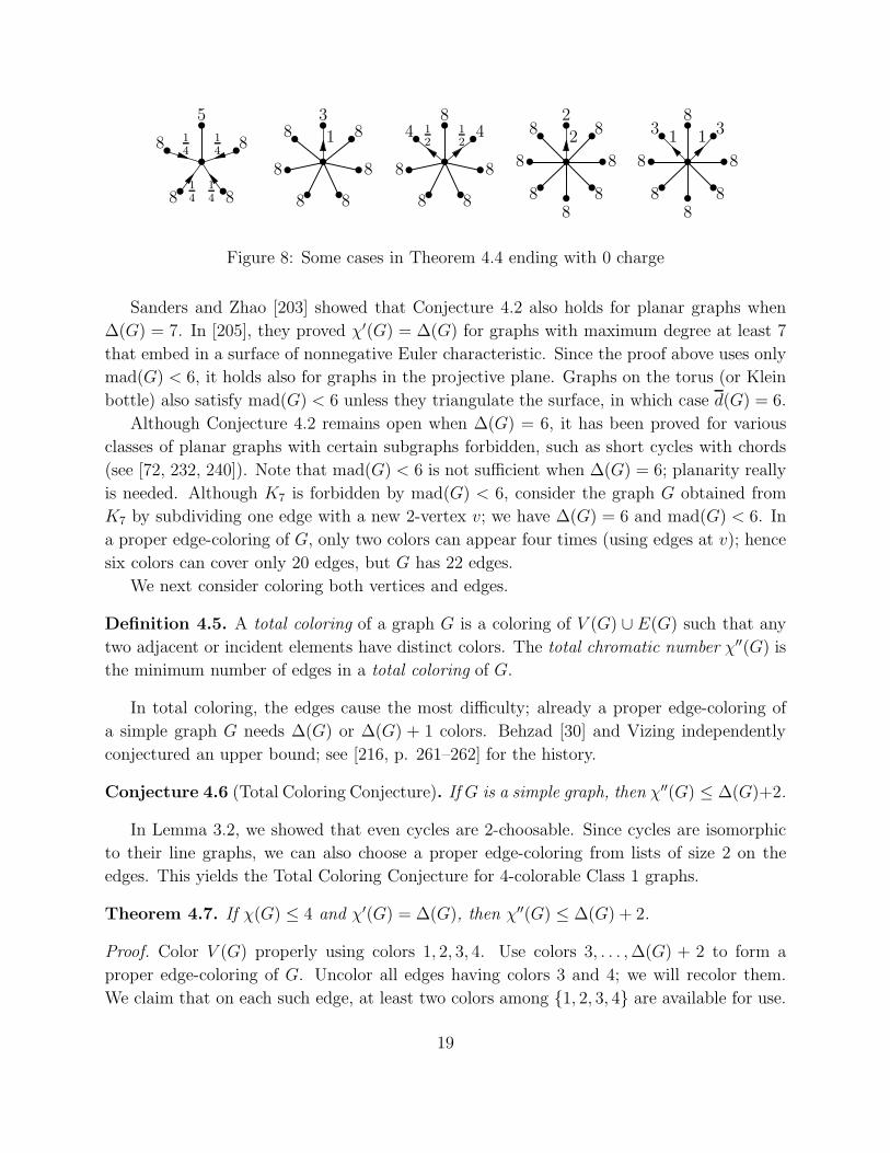
The remaining cases are all similar but require individual checking. We show represen-
tative cases in Figure 8.
If d(v) = 6, then j ≥ 4. At most j−3 neighbors have degree less than k. For j ∈ 4, 5, 6,v gives at most 2
4, 24, 34and receives at least 5
4, 44, 64, respectively, ending happy.
If d(v) = 7, then j ≥ 3. At most j − 2 neighbors have degree less than k. For j ∈3, 4, 5, 6, v gives at most 3
3, 44, 34, 44, respectively, and remains happy.
If d(v) ≥ 8, then j ≥ 2. At most j − 1 neighbors have degree less than k. For j ∈2, 3, 4, 5, 6, v gives at most 4
2, 63, 64, 44, 54, respectively, and remains happy.
18
••
••
• •14
14
14
5
8
88
8
14
•••
••••
•8
8
88
8
83
1•
••
••••
•
8
8
88
8
4 412
12
• ••
•••••
•8
8
88
8
8
82
2• •
••••
••
•
8
8
88
8
8
3 31 1
Figure 8: Some cases in Theorem 4.4 ending with 0 charge
Sanders and Zhao [203] showed that Conjecture 4.2 also holds for planar graphs when
∆(G) = 7. In [205], they proved χ′(G) = ∆(G) for graphs with maximum degree at least 7
that embed in a surface of nonnegative Euler characteristic. Since the proof above uses only
mad(G) < 6, it holds also for graphs in the projective plane. Graphs on the torus (or Klein
bottle) also satisfy mad(G) < 6 unless they triangulate the surface, in which case d(G) = 6.
Although Conjecture 4.2 remains open when ∆(G) = 6, it has been proved for various
classes of planar graphs with certain subgraphs forbidden, such as short cycles with chords
(see [72, 232, 240]). Note that mad(G) < 6 is not sufficient when ∆(G) = 6; planarity really
is needed. Although K7 is forbidden by mad(G) < 6, consider the graph G obtained from
K7 by subdividing one edge with a new 2-vertex v; we have ∆(G) = 6 and mad(G) < 6. In
a proper edge-coloring of G, only two colors can appear four times (using edges at v); hence
six colors can cover only 20 edges, but G has 22 edges.
We next consider coloring both vertices and edges.
Definition 4.5. A total coloring of a graph G is a coloring of V (G) ∪ E(G) such that any
two adjacent or incident elements have distinct colors. The total chromatic number χ′′(G) is
the minimum number of edges in a total coloring of G.
In total coloring, the edges cause the most difficulty; already a proper edge-coloring of
a simple graph G needs ∆(G) or ∆(G) + 1 colors. Behzad [30] and Vizing independently
conjectured an upper bound; see [216, p. 261–262] for the history.
Conjecture 4.6 (Total Coloring Conjecture). If G is a simple graph, then χ′′(G) ≤ ∆(G)+2.
In Lemma 3.2, we showed that even cycles are 2-choosable. Since cycles are isomorphic
to their line graphs, we can also choose a proper edge-coloring from lists of size 2 on the
edges. This yields the Total Coloring Conjecture for 4-colorable Class 1 graphs.
Theorem 4.7. If χ(G) ≤ 4 and χ′(G) = ∆(G), then χ′′(G) ≤ ∆(G) + 2.
Proof. Color V (G) properly using colors 1, 2, 3, 4. Use colors 3, . . . ,∆(G) + 2 to form a
proper edge-coloring of G. Uncolor all edges having colors 3 and 4; we will recolor them.
We claim that on each such edge, at least two colors among 1, 2, 3, 4 are available for use.
19
The colored edges exclude no colors, because now none of them have any color in 1, 2, 3, 4.The only vertices that can exclude a color from use on an edge are its endpoints.
Now lists of size 2 are available on the edges. The graph consisting of edges that had
colors 3 or 4 has maximum degree at most 2, so it consists of paths and even cycles, and a
proper edge-coloring can be chosen from the lists.
Using Theorem 4.7, the results on Vizing’s Planar Graph Conjecture, and the 4-colorability
of planar graphs (discussed briefly in Section 5), the Total Coloring Conjecture has almost
been proved for planar graphs. The cases with ∆(G) ≤ 5 were proved by ad hoc arguments.
Since χ′(G) = ∆(G) when G is planar with ∆(G) ≥ 7, Theorem 4.7 applies in that case.
Thus only the case ∆(G) = 6 remains unsettled for planar graphs. The bound is sharp, since
χ′′(K4) = 5. However, Borodin [39] proved χ′′(G) = ∆(G) + 1 when G is a simple planar
graph with ∆(G) ≥ 14, equaling the trivial lower bound (see Exercise 5.6).
Proper edge-coloring of G is equivalent to proper coloring of the line graph L(G). Since
the line graph has a clique of size ∆(G), Vizing’s Theorem states that the optimization
problem of proper coloring behaves much better when restricted to line graphs. The same
phenomenon seems to occur with the list version of the problem.
Definition 4.8. An edge-list assignment L assigns lists of available colors to the edges of a
graph G. Given an edge-list assignment L, an L-edge-coloring of G is a proper edge-coloring
φ such that φ(e) ∈ L(e) for all e ∈ E(G). A graph G is k-edge-choosable if G is L-edge-
colorable whenever each list has size at least k. The list edge-chromatic number of G, written
χ′ℓ(G), is the least k such that G is k-edge-choosable.
Conjecture 4.9 (List Coloring Conjecture). χ′ℓ(G) = χ′(G) for every graph G.
This conjecture was posed independently by many researchers. It was first published
by Bollobas and Harris [32], but it was independently formulated earlier by Albertson and
Collins in 1981 and by Vizing as early as 1975 (both unpublished). Vizing also posed
the weaker conjecture that always χ′ℓ(G) ≤ ∆(G) + 1. Kahn [144] proved the conjecture
asymptotically: χ′ℓ(G) ≤ (1 + o(1))χ′(G).
The List Coloring Conjecture was proved for bipartite multigraphs by Galvin [119],
showing that χ′ℓ(G) = ∆(G). Vizing [226, 227] conjectured that χ′(G) = ∆(G) when
mad(G) < ∆(G) − 1. Based on the List Coloring Conjecture, Woodall [246] conjectured
that mad(G) < ∆(G) − 1 also implies χ′ℓ(G) = ∆(G). In this direction, it is known that
χ′ℓ(G) = ∆(G) when mad(G) <
√
2∆(G). The result is implicit in [67], using the tool below.
Woodall [246] reinterpreted the argument in the language of discharging.
Theorem 4.10 (Borodin–Kostochka–Woodall [67]). If L is an edge-list assignment on a
bipartite multigraph G such that |L(uv)| ≥ maxdG(u), dG(v) for all uv ∈ E(G), then G
has an L-edge-coloring.
20
Woodall [246] introduced an exciting new technique of moving charge in successive stages
rather than all at once. When the average degree is large, vertices with very small degree
need a lot of charge. It may be too complicated to specify exactly where it all comes from.
Hence he allows charge to shift in phases, which we call “iterated discharging”.
We start with the reducible configurations. The weight of an edge inG (or of any subgraph
H) is the sum of the degrees (in G) of its vertices. When the weight of a subgraph satisfies
a desired bound, we say that the subgraph is light in G.
Proposition 4.11. Edges of weight at most k + 1 are reducible for k-edge-choosability.
Proof. A light edge e is incident to at most k − 1 edges. If G − e is k-edge-choosable and
|L(e)| ≥ k, then an L-edge-coloring of G− e extends to an L-edge-coloring of G.
For the other reducible configuration, we need a definition.
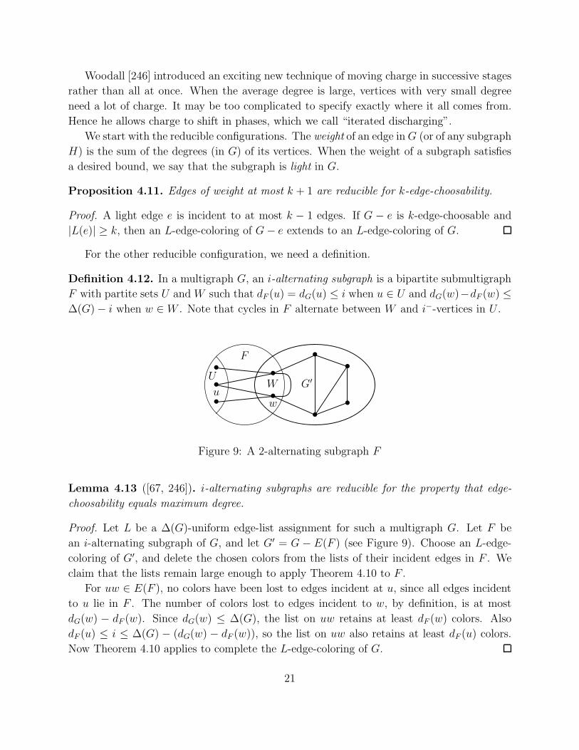
Definition 4.12. In a multigraph G, an i-alternating subgraph is a bipartite submultigraph
F with partite sets U and W such that dF (u) = dG(u) ≤ i when u ∈ U and dG(w)−dF (w) ≤∆(G)− i when w ∈ W . Note that cycles in F alternate between W and i−-vertices in U .
•••
•
••
•
•
•
F
G′
uw
UW
Figure 9: A 2-alternating subgraph F
Lemma 4.13 ([67, 246]). i-alternating subgraphs are reducible for the property that edge-
choosability equals maximum degree.
Proof. Let L be a ∆(G)-uniform edge-list assignment for such a multigraph G. Let F be
an i-alternating subgraph of G, and let G′ = G − E(F ) (see Figure 9). Choose an L-edge-
coloring of G′, and delete the chosen colors from the lists of their incident edges in F . We
claim that the lists remain large enough to apply Theorem 4.10 to F .
For uw ∈ E(F ), no colors have been lost to edges incident at u, since all edges incident
to u lie in F . The number of colors lost to edges incident to w, by definition, is at most
dG(w) − dF (w). Since dG(w) ≤ ∆(G), the list on uw retains at least dF (w) colors. Also
dF (u) ≤ i ≤ ∆(G) − (dG(w) − dF (w)), so the list on uw also retains at least dF (u) colors.
Now Theorem 4.10 applies to complete the L-edge-coloring of G.
21
To avoid technicalities, we make the bound on mad(G) slightly tighter than needed.
Theorem 4.14 ([67, 246]). If mad(G) ≤√
2∆(G)− 1, then χ′ℓ(G) = ∆(G).
Proof. Let x =√
2∆(G) − 1. It suffices to show that every graph G with average degree
at most x contains a edge with weight at most ∆(G) + 1 or an i-alternating subgraph with
i ≤ x. Suppose that G contains neither. An edge incident to a 1-vertex would be light, so
we may assume δ(G) ≥ 2.
Give each vertex initial charge equal to its degree. In phase i of discharging, for 2 ≤ i ≤⌊x⌋, each i−-vertex receives charge 1 from a neighbor. We design these phases so that every
vertex ends with charge at least ⌈x⌉.To begin phase i, let U = v : dG(v) ≤ i, and let W be the set of all vertices having
neighbors in U . Note that U is independent (no light edge). Let F be the subgraph with
vertex set U ∪W containing all edges incident to U . Since G has no i-alternating subgraph,
there exists w ∈ W such that dF (w) ≤ dG(w) + i −∆(G)− 1 ≤ i − 1. Move charge 1 from
this vertex w to each of its neighbors in U .
Now delete w ∪ (N(w) ∩ U) from F . Each deleted vertex in U has received charge 1,
and w lost at most i − 1. Iterate. What remains of U and W at each step cannot form an
i-alternating subgraph, so we continue to find the desired vertex until U is empty.
Since each vertex with degree at most i receives a unit of charge in phase i, vertices with
degree less than√
2∆(G) have their charge increased to at least√
2∆(G) (and they never
lose charge). Since there is no light edge, vertices with larger degree j lose charge only on
rounds i with i ≥ ∆(G)+2−j. Hence such a vertex loses charge at most∑⌊x⌋
i=∆(G)+2−j(i−1).
With each reduction of 1 in j, the amount of lost charge declines by more than 1, so it suffices
to show that vertices with degree ∆(G) keep sufficient charge. Their lost charge is bounded
by 12x(x− 1), so they keep charge at least 3
2
√
2∆(G)− 1, which is more than enough.
Woodall also gave an example to show that the discharging argument is essentially sharp,
meaning that more reducible configurations will be needed to weaken the hypothesis on
mad(G). By using VAL and further adjacency lemmas to study the relationship between
criticality for Class 1 and mad(G), Sanders and Zhao [204] proved that mad(G) < 12∆(G)
suffices to make G Class 1, and Woodall [245] proved that mad(G) < 23∆(G) suffices. The list
version seems to be much harder, and the more restrictive requirement of mad(G) <√
2∆(G)
in Theorem 4.14 is a first step.
Exercise 4.1. Let G be a graph with maximum degree at least 8 that embeds on the torus. Bya closer examination of the proof of Theorem 4.4, prove that χ′(G) = ∆(G) except possibly whenG is obtained from a 6-regular triangulation H of the torus by inserting vertices of degree 3 intoone-third of the faces in H, chosen so that each vertex in H lies on exactly two of the chosen faces,and making each new vertex adjacent to the vertices of H on its face. It suffices to show thatotherwise every vertex ends with charge at least 6 and some vertex ends with larger charge.
22
Exercise 4.2. Prove that if ∆(G) ≤ 6 and d(G) < 72 , then G contains an isolated vertex, an edge
with weight at most 7, or a cycle alternating between 2-vertices and 6-vertices. Conclude that if∆(G) ≤ 6 and mad(G) < 7
2 , then G is 6-edge-choosable and 7-total-choosable.
Exercise 4.3. (Borodin–Kostochka–Woodall [67]) Adapt the proofs of Lemma 4.13 and Theo-rem 4.14 to show that if mad(G) ≤
√
2∆(G) − 1, then χ′′ℓ (G) = ∆(G) + 1.
5 Planar Graphs and Coloring
The Discharging Method was developed in the study of planar graphs. Although many
results on planar graphs (especially with girth restrictions) extend to all graphs satisfying
the resulting bound on mad(G), in this section we return to the historical roots and emphasize
results where planarity is needed. Since planarity is very restrictive, for planar graphs one
can sometimes prove stronger results than hold for mad(G) < 6. As examples, we first
pursue the problems discussed in Section 4 (other examples appear in the exercises).
Borodin [41] confirmed the List Coloring Conjecture for planar graphs with large maxi-
mum degree, proving that χ′ℓ(G) = ∆(G) when ∆(G) ≥ 14. This later was strengthened to
∆(G) ≥ 12 by Borodin, Kostochka, and Woodall [67]. Borodin [41] also confirmed Vizing’s
weaker conjecture in the broader class of planar graphs with ∆(G) ≥ 9, showing that then
χ′ℓ(G) ≤ ∆(G) + 1. Bonamy [33] obtained this conclusion also for ∆(G) = 8, by a much
longer proof using 11 reducible configurations.
The bound ∆(G) + 1 has also been proved for planar graphs with ∆(G) ≥ 6 having no
two 3-faces sharing an edge [89]. It was proved in [143] for ∆(G) ≤ 4 (including nonplanar
graphs), and when ∆(G) = 5 it is known for planar graphs with no 3-cycle [255], no 4-
cycle [89], or no 5-cycle [233]. The proofs for ∆(G) = 5 all use discharging.
The distinctive feature of discharging for planar graphs is that charge can also be assigned
to faces, which are vertices in the dual graph. The dual graphG∗ is also planar, so mad(G∗) <
6 and we can use discharging on both G and G∗. Using their interaction is more effective
and leads to three common (and natural) ways to assign charge on planar graphs.
Proposition 5.1. Let V (G) and F (G) be the sets of vertices and faces in a plane graph G,
and let ℓ(f) denote the length of a face f . The following equalities hold for G.∑
v∈V (G)(d(v)− 6) +∑
f∈F (G)(2ℓ(f)− 6) = −12 vertex charging∑
v∈V (G)(2d(v)− 6) +∑
f∈F (G)(ℓ(f)− 6) = −12 face charging∑
v∈V (G)(d(v)− 4) +∑
f∈F (G)(ℓ(f)− 4) = −8 balanced charging
Proof. Euler’s Formula for connected planar graphs is n − m + p = 2, where n, m, and p
count the vertices, edges, and faces (“points” in the dual). Multiply Euler’s Formula by −6
or −4 and split the term for edges to obtain the three formulas below.
−6n+ 2m+ 4m− 6p = −12; −6n+ 4m+ 2m− 6f = −12; −4n+ 2m+ 2m− 4f = −8.
23
Substitute 12
∑
v∈V (G) d(v) for the first occurrence of m and 12
∑
f∈F (G) ℓ(f) for the second in
each equation, and then collect the contributions by vertices and by faces.
Here the initial charges assigned to vertices or faces are not the degree or length, but
rather an adjustment of those quantities that uses the interaction between vertices and faces.
Setting charge to degree is in some sense more intuitive, but this adjustment facilitates using
the dual graph also. A vertex or face now is “happy” when it reaches nonnegative charge.
When specified configurations are assumed not to occur, making every vertex and face happy
provides a contradiction in the same way as when charges are not shifted.
For triangulations, such as in the Four Color Problem, vertex charging is appropriate.
All the faces have charge 0, and often they can be ignored. For 3-regular planar graphs, face
charging is appropriate, with each vertex given charge 0. With balanced charging when G
and its dual G∗ are simple, 3-vertices and 3-faces are the only objects needing charge; those
with degree or length at least 5 have spare charge to give away.
We begin with the recent use of balanced charging to prove the result of Borodin [41]
on Vizing’s List Edge-Coloring Conjecture for planar graphs with large degree. Balanced
charging is natural when neither the graphs nor their duals are triangulations. An interesting
aspect of the proof is a reservoir or “pot” of charge that can flow to or from vertices or
faces without regard to their location. In this proof, the pot facilitates moving charge from
maximum-degree vertices to 3-vertices; we need not name specific recipients.
Theorem 5.2 ([41]). If G is a planar graph and ∆(G) ≥ 9, then χ′ℓ(G) ≤ ∆(G) + 1.
Proof. (Cohen and Havet [84]) Let G be a minimal counterexample, with an edge-list as-
signment L such that each list has size ∆(G) + 1 and G has no L-edge-coloring. An edge
with weight at most ∆(G) + 2 is reducible, by Proposition 4.11. Hence we may assume
that δ(G) ≥ 3 and that every neighbor of a j-vertex has degree at least ∆(G) + 3 − j. Let
k = ∆(G); since k ≥ 9, the degree-sum of any two adjacent vertices is at least 12.
We use balanced charging, with initial charge equal to degree or length minus 4. Initially,
the pot of charge is empty. The discharging rules must make each vertex and face happy and
keep the charge in the pot nonnegative to contradict the assumption of a counterexample.
(R1) Every 3-vertex takes 1 from the pot, and every k-vertex gives 12to the pot.
(R2) Each 3-face takes 12from each incident 8+-vertex and j−4
jfrom each incident j-vertex
with j ∈ 5, 6, 7.To ensure positive charge in the pot, we prove nk > 2n3, where nj is the number of
j-vertices in G. The edges incident to 3-vertices form a bipartite graph H ; its partite sets
are the 3-vertices and the k-vertices. If H has a cycle C, then C has even length, since H is
bipartite. By the minimality of the counterexample, G−E(C) has an L-edge-coloring. Each
edge of C is incident to ∆(G)−1 edges that have now been colored, so there remain at least
24
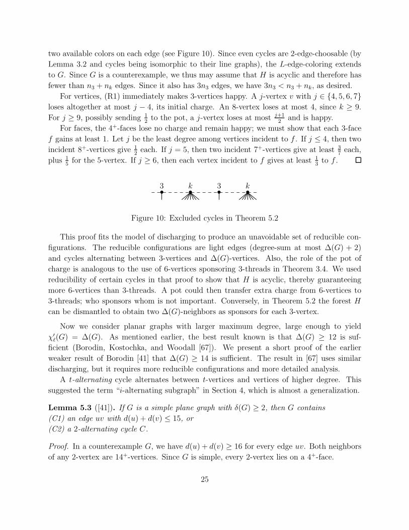
two available colors on each edge (see Figure 10). Since even cycles are 2-edge-choosable (by
Lemma 3.2 and cycles being isomorphic to their line graphs), the L-edge-coloring extends
to G. Since G is a counterexample, we thus may assume that H is acyclic and therefore has
fewer than n3 + nk edges. Since it also has 3n3 edges, we have 3n3 < n3 + nk, as desired.
For vertices, (R1) immediately makes 3-vertices happy. A j-vertex v with j ∈ 4, 5, 6, 7loses altogether at most j − 4, its initial charge. An 8-vertex loses at most 4, since k ≥ 9.
For j ≥ 9, possibly sending 12to the pot, a j-vertex loses at most j+1
2and is happy.
For faces, the 4+-faces lose no charge and remain happy; we must show that each 3-face
f gains at least 1. Let j be the least degree among vertices incident to f . If j ≤ 4, then two
incident 8+-vertices give 12each. If j = 5, then two incident 7+-vertices give at least 3
7each,
plus 15for the 5-vertex. If j ≥ 6, then each vertex incident to f gives at least 1
3to f .
• • • •3 k 3 k
Figure 10: Excluded cycles in Theorem 5.2
This proof fits the model of discharging to produce an unavoidable set of reducible con-
figurations. The reducible configurations are light edges (degree-sum at most ∆(G) + 2)
and cycles alternating between 3-vertices and ∆(G)-vertices. Also, the role of the pot of
charge is analogous to the use of 6-vertices sponsoring 3-threads in Theorem 3.4. We used
reducibility of certain cycles in that proof to show that H is acyclic, thereby guaranteeing
more 6-vertices than 3-threads. A pot could then transfer extra charge from 6-vertices to
3-threads; who sponsors whom is not important. Conversely, in Theorem 5.2 the forest H
can be dismantled to obtain two ∆(G)-neighbors as sponsors for each 3-vertex.
Now we consider planar graphs with larger maximum degree, large enough to yield
χ′ℓ(G) = ∆(G). As mentioned earlier, the best result known is that ∆(G) ≥ 12 is suf-
ficient (Borodin, Kostochka, and Woodall [67]). We present a short proof of the earlier
weaker result of Borodin [41] that ∆(G) ≥ 14 is sufficient. The result in [67] uses similar
discharging, but it requires more reducible configurations and more detailed analysis.
A t-alternating cycle alternates between t-vertices and vertices of higher degree. This
suggested the term “i-alternating subgraph” in Section 4, which is almost a generalization.
Lemma 5.3 ([41]). If G is a simple plane graph with δ(G) ≥ 2, then G contains
(C1) an edge uv with d(u) + d(v) ≤ 15, or
(C2) a 2-alternating cycle C.
Proof. In a counterexample G, we have d(u) + d(v) ≥ 16 for every edge uv. Both neighbors
of any 2-vertex are 14+-vertices. Since G is simple, every 2-vertex lies on a 4+-face.
25
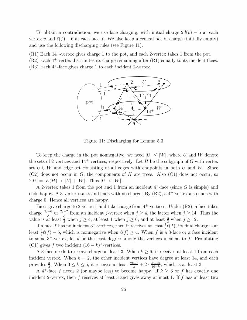
To obtain a contradiction, we use face charging, with initial charge 2d(v) − 6 at each
vertex v and ℓ(f)− 6 at each face f . We also keep a central pot of charge (initially empty)
and use the following discharging rules (see Figure 11).
(R1) Each 14+-vertex gives charge 1 to the pot, and each 2-vertex takes 1 from the pot.
(R2) Each 4+-vertex distributes its charge remaining after (R1) equally to its incident faces.
(R3) Each 4+-face gives charge 1 to each incident 2-vertex.
•
•
•
•
•
pot
W
U2 2
14+14+
1
1
1
1
1 1 1
Figure 11: Discharging for Lemma 5.3
To keep the charge in the pot nonnegative, we need |U | ≤ |W |, where U and W denote
the sets of 2-vertices and 14+-vertices, respectively. Let H be the subgraph of G with vertex
set U ∪ W and edge set consisting of all edges with endpoints in both U and W . Since
(C2) does not occur in G, the components of H are trees. Also (C1) does not occur, so
2|U | = |E(H)| < |U |+ |W |. Thus |U | < |W |.A 2-vertex takes 1 from the pot and 1 from an incident 4+-face (since G is simple) and
ends happy. A 3-vertex starts and ends with no charge. By (R2), a 4+-vertex also ends with
charge 0. Hence all vertices are happy.
Faces give charge to 2-vertices and take charge from 4+-vertices. Under (R2), a face takes
charge 2j−6j
or 2j−7j
from an incident j-vertex when j ≥ 4, the latter when j ≥ 14. Thus the
value is at least 12when j ≥ 4, at least 1 when j ≥ 6, and at least 3
2when j ≥ 12.
If a face f has no incident 3−-vertices, then it receives at least 12ℓ(f); its final charge is at
least 32ℓ(f)− 6, which is nonnegative when ℓ(f) ≥ 4. When f is a 3-face or a face incident
to some 3−-vertex, let k be the least degree among the vertices incident to f . Prohibiting
(C1) gives f two incident (16− k)+-vertices.
A 3-face needs to receive charge at least 3. When k ≥ 6, it receives at least 1 from each
incident vertex. When k = 2, the other incident vertices have degree at least 14, and each
provides 32. When 3 ≤ k ≤ 5, it receives at least 2k−6
k+ 2 · 26−2k
16−k, which is at least 3.
A 4+-face f needs 2 (or maybe less) to become happy. If k ≥ 3 or f has exactly one
incident 2-vertex, then f receives at least 3 and gives away at most 1. If f has at least two
26
incident 2-vertices, then each is followed on f (in a consistent direction) by a 14+-vertex,
which contributes at least 32. These pairs net at least 1
2each for f . If G has no 2-alternating
cycle, then f has another incident 14+-vertex that has not been counted, which provides
more than enough charge to f .
Theorem 5.4 ([41]). If G is a plane graph with ∆(G) ≥ 14, then χ′ℓ(G) = ∆(G).
Proof. Let G be a minimal counterexample, having no L-edge-coloring from edge-list assign-
ment L. If G has a 1-vertex with incident edge e, then G − e has an L-edge-coloring, and
it extends to e. Thus δ(G) ≥ 2. By Lemma 5.3, G has an edge uv with d(u) + d(v) ≤ 15
or a 2-alternating cycle C. In the first case, we can extend an L-edge-coloring of G − uv,
since |L(uv)| ≥ 14 and at most 13 colors are restricted from use on uv. In the other case,
by minimality G−E(C) has an L-edge-coloring. Since each list has size at least ∆(G), each
edge of C has at least two colors remaining available, and the 2-choosability of even cycles
allows us to extend the edge-coloring.
We close this section with a new proof of a classical result that appeared in the survey [45]
with the traditional proof. Steinberg [215] conjectured that every planar graph without 4-
cycles or 5-cycles is 3-colorable. Results on this family can be compared with the family
where mad(G) < 4; see Exercise 5.7.
Many papers have used discharging to prove 3-colorability under various excluded-cycle
conditions. For example, Borodin et al. [51] proved that excluding cycles of lengths 4 through
7 suffices. Earlier, Borodin [43] and Sanders and Zhao [200] proved that excluding 4-cycles
and faces of lengths 5 through 9 is sufficient. The traditional proof uses balanced charging,
but face charging yields a somewhat simpler proof.
Lemma 5.5 ([43]). Every plane graph G with δ(G) ≥ 3 has two 3-faces with a common
edge, or a j-face with 4 ≤ j ≤ 9, or a 10-face whose vertices all have degree 3.
Proof. Let G be a plane graph with δ(G) ≥ 3 having none of the listed configurations. Use
face charging: assign charge 2d(v)− 6 to each vertex v and charge ℓ(f)− 6 to each face f .
The total charge is −12.
Since no faces have lengths 4 through 9, the only objects with initial negative charge are
triangles; they begin with charge −3. Each triangle takes 1 from each neighboring face. To
repair faces that may lose too much, each face f takes 1 from each incident 4+-vertex lying
on at least one triangle sharing an edge with f (see Figure 12).
We have made 3-faces happy, and 3-vertices remain at charge 0. Other vertices remain
happy because 3-faces do not share edges. For j ≥ 4, a j-vertex loses charge at most⌊
j2
⌋
and ends with at least⌈
3j2
⌉
− 6, which is nonnegative for j ≥ 4.
Now consider a j-face f for j ≥ 10. It loses 1 for every path along its boundary such
that the neighboring faces are triangles and the endpoints have degree 3; f gives 1 to each
27
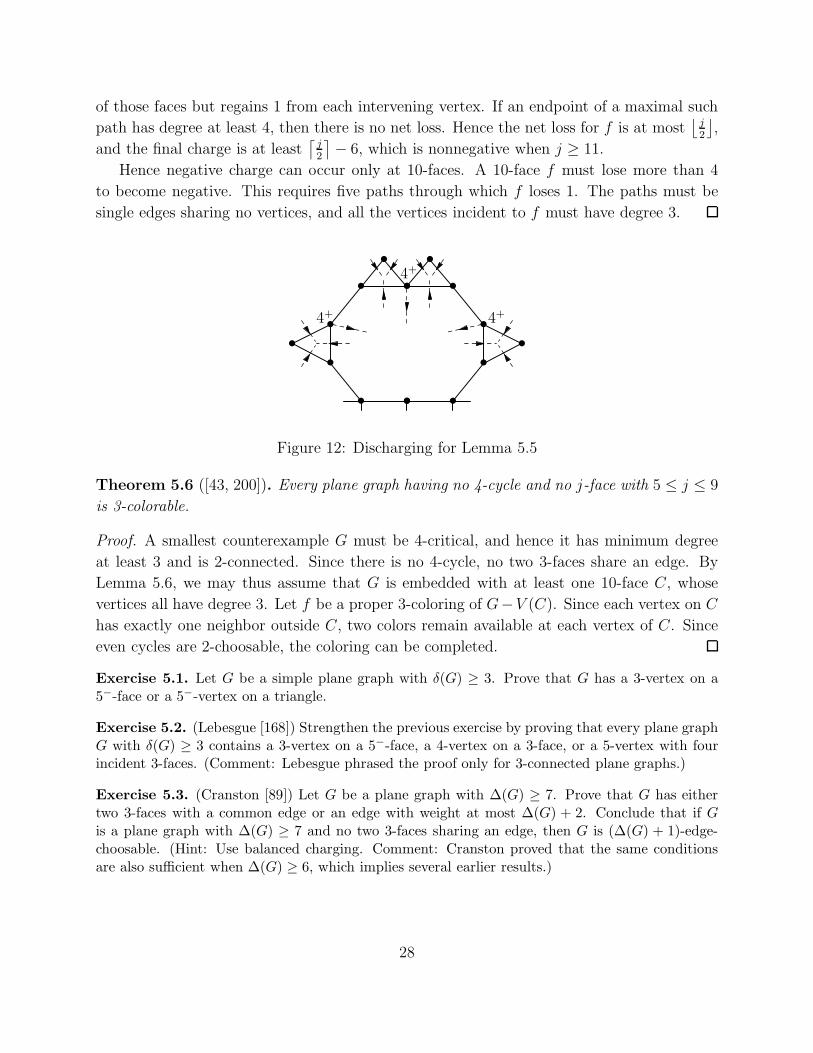
of those faces but regains 1 from each intervening vertex. If an endpoint of a maximal such
path has degree at least 4, then there is no net loss. Hence the net loss for f is at most⌊
j2
⌋
,
and the final charge is at least⌈
j2
⌉
− 6, which is nonnegative when j ≥ 11.
Hence negative charge can occur only at 10-faces. A 10-face f must lose more than 4
to become negative. This requires five paths through which f loses 1. The paths must be
single edges sharing no vertices, and all the vertices incident to f must have degree 3.
• •
••
•
••
•
••
••
•
••
•
4+
4+
4+
Figure 12: Discharging for Lemma 5.5
Theorem 5.6 ([43, 200]). Every plane graph having no 4-cycle and no j-face with 5 ≤ j ≤ 9
is 3-colorable.
Proof. A smallest counterexample G must be 4-critical, and hence it has minimum degree
at least 3 and is 2-connected. Since there is no 4-cycle, no two 3-faces share an edge. By
Lemma 5.6, we may thus assume that G is embedded with at least one 10-face C, whose
vertices all have degree 3. Let f be a proper 3-coloring of G−V (C). Since each vertex on C
has exactly one neighbor outside C, two colors remain available at each vertex of C. Since
even cycles are 2-choosable, the coloring can be completed.
Exercise 5.1. Let G be a simple plane graph with δ(G) ≥ 3. Prove that G has a 3-vertex on a5−-face or a 5−-vertex on a triangle.
Exercise 5.2. (Lebesgue [168]) Strengthen the previous exercise by proving that every plane graphG with δ(G) ≥ 3 contains a 3-vertex on a 5−-face, a 4-vertex on a 3-face, or a 5-vertex with fourincident 3-faces. (Comment: Lebesgue phrased the proof only for 3-connected plane graphs.)
Exercise 5.3. (Cranston [89]) Let G be a plane graph with ∆(G) ≥ 7. Prove that G has eithertwo 3-faces with a common edge or an edge with weight at most ∆(G) + 2. Conclude that if Gis a plane graph with ∆(G) ≥ 7 and no two 3-faces sharing an edge, then G is (∆(G) + 1)-edge-choosable. (Hint: Use balanced charging. Comment: Cranston proved that the same conditionsare also sufficient when ∆(G) ≥ 6, which implies several earlier results.)
28
Exercise 5.4. Prove that every plane triangulation with minimum degree 5 has two 3-faces sharingan edge such that the non-shared vertices have degree-sum at most 11. (Hint: Use vertex charging;6-vertices that give charge to 5-neighbors will need charge from 7+-neighbors. Comment: Albert-son [6] used this configuration in a proof that α(G) ≥ 2n
9 when G is an n-vertex planar graph withno separating triangle, without using the Four Color Theorem or the language of discharging.)
Exercise 5.5. (Dvorak, Kawarabayashi, and Thomas [101]) Let C be the outer boundary in a2-connected triangle-free plane graph G that is not a cycle. If C has length at most 6, and everyvertex not on C has degree at least 3, then G contains a bounded 4-face or a proper 5-face, wherea 5-face is proper if (at least) four of its vertices have degree 3 and are not on C. (Comment: Thisresult was used in [101] to give a new proof of Grotzsch’s Theorem [122] that triangle-free planargraphs are 3-colorable. The proof in [101] used vertex charging, but using face charging is simpler.)
Exercise 5.6. (Borodin [39]) Using Lemma 5.3, adapt the proof of Theorem 5.4 to show thatχ′′ℓ (G) = ∆(G) + 1 when G is a planar graph with ∆(G) ≥ 14.
Exercise 5.7. Let G be a plane graph having no 4-cycle and no face with length in 4, . . . , k.Use discharging to prove that the average face length in G is at least 6 − 18
k+4 . Conclude that
mad(G) < 3+ 92k−1 . In particular, mad(G) < 4 when G is a plane graph having no 4-face or 5-face.
6 Light Subgraphs of Planar Graphs
We have noted that in inductive proofs for χ′ℓ(G) ≤ k, a light edge uv (that is, satisfying
dG(u) + dG(v) ≤ k + 1) is reducible, since extending a proper edge-coloring of G− uv to G
only requires the color on uv to avoid the colors on k − 1 other edges. Planar graphs are
also guaranteed to have light copies of other subgraphs, often by discharging.
The Four Color Theorem begins with light subgraphs — specifically, light vertices. A pla-
nar graph has a 5−-vertex. After showing that 4−-vertices are reducible for proper 4-coloring,
attention turns to triangulations with minimum degree 5. Wernicke [243] guaranteed an edge
with weight at most 11 in such a graph; in Lemma 6.1 we will prove more. Further light sub-
graphs (and other configurations) are generated via discharging rules, and we seek reducible
configurations. Unfortunately, the details become rather complicated.
The initial proof by Appel and Haken (working with Koch) involved 1936 reducible
configurations. The unavoidable set was generated by hand, but the details of proving
reducibility were so lengthy that they were checked by computer. The publication comprised
nearly 140 pages in two papers [13, 20] plus over 400 pages of microfiche [14, 15]. With further
explanations, this became a 741-page book [19] (see also [18]).
Some researchers objected to the use of computers. Robertson, Sanders, Seymour, and
Thomas [196] looked for a simpler proof; they wound up using the same approach. Their
unavoidable set had only 633 configurations and 32 discharging rules, but they still needed a
computer. With a faster computer and simpler arguments, their proof ran in only 20 minutes
instead of the original 1200 hours.
29
Not all parts of these proofs are hopelessly complicated. Appel and Haken [17] published a
shorter paper with simpler discharging to prove that for planar triangulations with minimum
degree 5 but no adjacent 5-vertices there is an unavoidable set of 47 configurations likely to
be reducible; in [21] there is an even shorter such list, whose reducibility they showed.
Stronger results later followed. Robertson, Seymour, and Thomas [197] used the Four
Color Theorem (in a paper that won the 1994 Fulkerson Prize) to prove the case k = 6 of
Hadwiger’s Conjecture: graphs not having K6 as a minor are 5-colorable (the case k = 5 is
equivalent to the Four Color Theorem, as shown by Wagner [229]).
Using the planar dual, Tait [217] showed that 4-colorability of planar triangulations is
equivalent to 3-edge-colorability of 3-regular 2-edge-connected planar graphs. Planar graphs
contain no subdivision of the (nonplanar) Petersen graph. Hence Tutte’s conjecture that
3-regular 2-edge-connected graphs containing no Petersen-subdivision are 3-edge-colorable
is stronger than the Four Color Theorem. In 2001, Robertson, Sanders, Seymour, and
Thomas announced a proof of this. First Robertson, Seymour, and Thomas [198] reduced the
conjecture to proving it for two special classes of graphs: “apex” graphs and “doublecross”
graphs. However, [198] relies on an unpublished manuscript [199]. Later, 3-edge-colorability
was proved for the two special classes by Sanders, Seymour, and Thomas, but this also has
not been published. In 2012, Seymour described this proof, with its reliance on discharging
and many reducible configurations, as “Repeat the proof of the 4CT (twice)”.
The Four Color Theorem uses discharging and reducibility as our examples do, but its
details remain too lengthy for discussion here. Instead, we will simply assume its correct-
ness and resume giving simpler results to explain various ideas and techniques that arise in
discharging proofs and their applications.
We continue with light subgraphs, a subject surveyed by Jendrol’ and Voss [140]. We
focus on light edges, which have been thoroughly studied. Edges are small enough that the
best bounds on the weight of light edges in various settings can be determined by discharging,
and yet they have many applications.
The best-known result on light edges is Kotzig’s Theorem [159]: every 3-connected planar
graph has an edge of weight at most 13. Borodin [39] later extended it. A normal plane
map is a plane multigraph such that every vertex degree and face length is at least 3; Euler’s
Formula holds also in this setting. Jendrol’ [139, 140] gave a short proof of the extension
that every normal plane map G has an edge with weight at most 11 or a 3-vertex with a 10−-
neighbor. Most applications of the lemma (including in this paper) use only this statement.
In fact, Borodin proved more. We extend the proof by Jendrol’ to obtain Borodin’s stronger
statement, which we will apply in Theorem 7.15. Discharging yields a short proof.
Lemma 6.1 (Borodin [39]). Every normal plane map G has an edge with weight at most 11
or a 4-cycle through two 3-vertices and a common 10−-neighbor.
Proof. If any face has length more than 3, then adding a chord does not create light edges
30
(it may create multi-edges). Hence we may assume that every face has length 3. Assume
that G has no light edge, and give initial charges by vertex charging.
(R1) Every 5− vertex v takes charge 6−d(v)d(v)
from each 7+-neighbor.
Since G is a triangulation without light edges, a k-vertex sends charge to at most⌊
k2
⌋
vertices. Since a 7-vertex sends charge only to 5-vertices, it loses at most 3 · 15and remains
positive. An 8-vertex sends charge only to 4+-vertices and loses at most 4 · 12, remaining
nonnegative. When d(v) ≥ 11, neighbors of v may have degree 3 and take charge 1, but the
final charge is at least⌈
d(v)2
⌉
− 6, again nonnegative.
Finally, suppose d(v) ∈ 9, 10. Since faces have length 3, the neighbors of v form a
closed walk of length d(v) when followed in order, and each 3-vertex appears only once in
this walk. With light edges and the specified 4-cycles forbidden, 3-vertices must be separated
by at least three steps along this walk.
Hence a 9-vertex has at most three 3-neighbors, and when it has three it ends with
charge 0, since it loses no other charge. Similarly it may have two 3-neighbors and up to
two 4-neighbors, reaching charge 0, or one 3-neighbor and up to three 4-neighbors, losing
charge at most 52. A 10-vertex may also have three 3-neighbors, or two 3-neighbors and three
4-neighbors, or other combinations losing less charge. The total charge lost is at most 72,
and the final charge is positive.
Further results on light edges for planar graphs with large girth appear in Lemma 6.11
and in Exercises 6.4–6.7. We will apply light edges in Theorems 6.3 and 6.10.
We discussed total coloring in Section 4. Now consider coloring vertices and faces instead
of vertices and edges. Ringel [195] conjectured the following theorem, proved by Borodin [37]
using discharging. The discharging argument produced a set of 35 configurations, all then
shown to be reducible (without computers). Borodin [42] later simplified the proof.
Theorem 6.2 (Borodin [37, 42]). The vertices and faces of any plane graph G can be colored
using six colors so that elements adjacent or incident in G or its dual receive different colors.
Beyond total coloring, an entire coloring of a plane graph G colors its vertices, edges, and
faces so that any two elements adjacent or incident in G or its dual have distinct colors. Let
χ′′′(G) be the least number of colors needed (also χV EF is used). Kronk and Mitchem [161]
introduced entire coloring and conjectured χ′′′(G) ≤ ∆(G) + 4 for every simple plane graph
G. Equality holds for K4 (see Figure 13). It seems unknown whether there are infinitely
many sharpness examples; perhaps fewer colors suffice when ∆(G) is sufficiently large.
This conjecture has been proved. It was proved for ∆(G) ≤ 3 by Kronk and Mitchem [162],
for ∆(G) ≥ 7 by Borodin [44], for ∆(G) = 6 by Sanders and Zhao [202] (corrected in [241]),
and for ∆(G) ∈ 4, 5 by Wang and Zhu [241]. Using Lemma 6.1 and the Four Color Theo-
rem, it is easy to prove the conjecture for ∆(G) ≥ 11 (see [38]; also Exercise 6.10 develops
another proof for ∆(G) ≥ 7). The crucial step is a list version of total coloring.
31
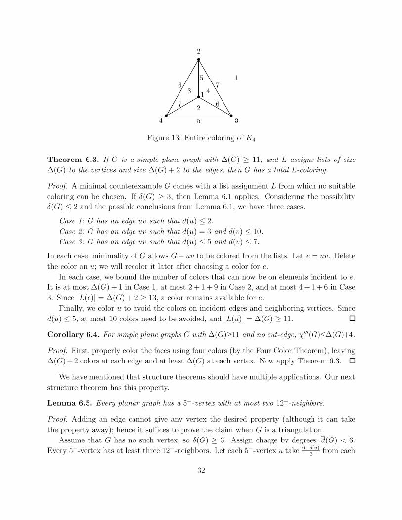
•
•
••
1
1
2
2
3
3
4
4
5
5
6
6 7
7
Figure 13: Entire coloring of K4
Theorem 6.3. If G is a simple plane graph with ∆(G) ≥ 11, and L assigns lists of size
∆(G) to the vertices and size ∆(G) + 2 to the edges, then G has a total L-coloring.
Proof. A minimal counterexample G comes with a list assignment L from which no suitable
coloring can be chosen. If δ(G) ≥ 3, then Lemma 6.1 applies. Considering the possibility
δ(G) ≤ 2 and the possible conclusions from Lemma 6.1, we have three cases.
Case 1: G has an edge uv such that d(u) ≤ 2.
Case 2: G has an edge uv such that d(u) = 3 and d(v) ≤ 10.
Case 3: G has an edge uv such that d(u) ≤ 5 and d(v) ≤ 7.
In each case, minimality of G allows G− uv to be colored from the lists. Let e = uv. Delete
the color on u; we will recolor it later after choosing a color for e.
In each case, we bound the number of colors that can now be on elements incident to e.
It is at most ∆(G) + 1 in Case 1, at most 2 + 1+ 9 in Case 2, and at most 4 + 1+ 6 in Case
3. Since |L(e)| = ∆(G) + 2 ≥ 13, a color remains available for e.
Finally, we color u to avoid the colors on incident edges and neighboring vertices. Since
d(u) ≤ 5, at most 10 colors need to be avoided, and |L(u)| = ∆(G) ≥ 11.
Corollary 6.4. For simple plane graphs G with ∆(G)≥11 and no cut-edge, χ′′′(G)≤∆(G)+4.
Proof. First, properly color the faces using four colors (by the Four Color Theorem), leaving
∆(G)+2 colors at each edge and at least ∆(G) at each vertex. Now apply Theorem 6.3.
We have mentioned that structure theorems should have multiple applications. Our next
structure theorem has this property.
Lemma 6.5. Every planar graph has a 5−-vertex with at most two 12+-neighbors.
Proof. Adding an edge cannot give any vertex the desired property (although it can take
the property away); hence it suffices to prove the claim when G is a triangulation.
Assume that G has no such vertex, so δ(G) ≥ 3. Assign charge by degrees; d(G) < 6.
Every 5−-vertex has at least three 12+-neighbors. Let each 5−-vertex u take 6−d(u)3
from each
32
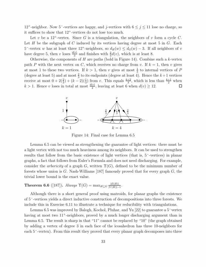
12+-neighbor. Now 5−-vertices are happy, and j-vertices with 6 ≤ j ≤ 11 lose no charge, so
it suffices to show that 12+-vertices do not lose too much.
Let v be a 12+-vertex. Since G is a triangulation, the neighbors of v form a cycle C.
Let H be the subgraph of C induced by its vertices having degree at most 5 in G. Each
5−-vertex w has at least three 12+-neighbors, so dH(w) ≤ dG(w) − 3. If all neighbors of v
have degree 5, then v loses d(v)3
and finishes with 23d(v), which is at least 8.
Otherwise, the components of H are paths (bold in Figure 14). Combine such a k-vertex
path P with the next vertex on C, which receives no charge from v. If k = 1, then v gives
at most 1 to these two vertices. If k > 1, then v gives at most 13to internal vertices of P
(degree at least 5) and at most 23to its endpoints (degree at least 4). Hence the k+1 vertices
receive at most 0 + 2(23) + (k − 2)(1
3) from v. This equals k+2
3, which is less than k+1
2when
k > 1. Hence v loses in total at most d(v)2, leaving at least 6 when d(v) ≥ 12.
•
• •
v
1
k = 1
•
• • • • •
v
13
k = 4
23
23
Figure 14: Final case for Lemma 6.5
Lemma 6.5 can be viewed as strengthening the guarantee of light vertices: there must be
a light vertex with not too much heaviness among its neighbors. It can be used to strengthen
results that follow from the basic existence of light vertices (that is, 5−-vertices) in planar
graphs, a fact that follows from Euler’s Formula and does not need discharging. For example,
consider the arboricity of a graph G, written Υ(G), defined to be the minimum number of
forests whose union is G. Nash-Williams [187] famously proved that for every graph G, the
trivial lower bound is the exact value.
Theorem 6.6 ([187]). Always Υ(G) = maxH⊆G|E(H)|
|V (H)|−1.
Although there is a short general proof using matroids, for planar graphs the existence
of 5−-vertices yields a direct inductive construction of decompositions into three forests. We
include this in Exercise 6.11 to illustrate a technique for reducibility with triangulations.
Lemma 6.5 was improved by Balogh, Kochol, Pluhar, and Yu [22] to guarantee a 5−vertex
having at most two 11+-neighbors, proved by a much longer discharging argument than in
Lemma 6.5. The result is sharp in that “11” cannot be replaced by “10” (the graph obtained
by adding a vertex of degree 3 in each face of the icosahedron has three 10-neighbors for
each 5−-vertex). From this result they proved that every planar graph decomposes into three
33
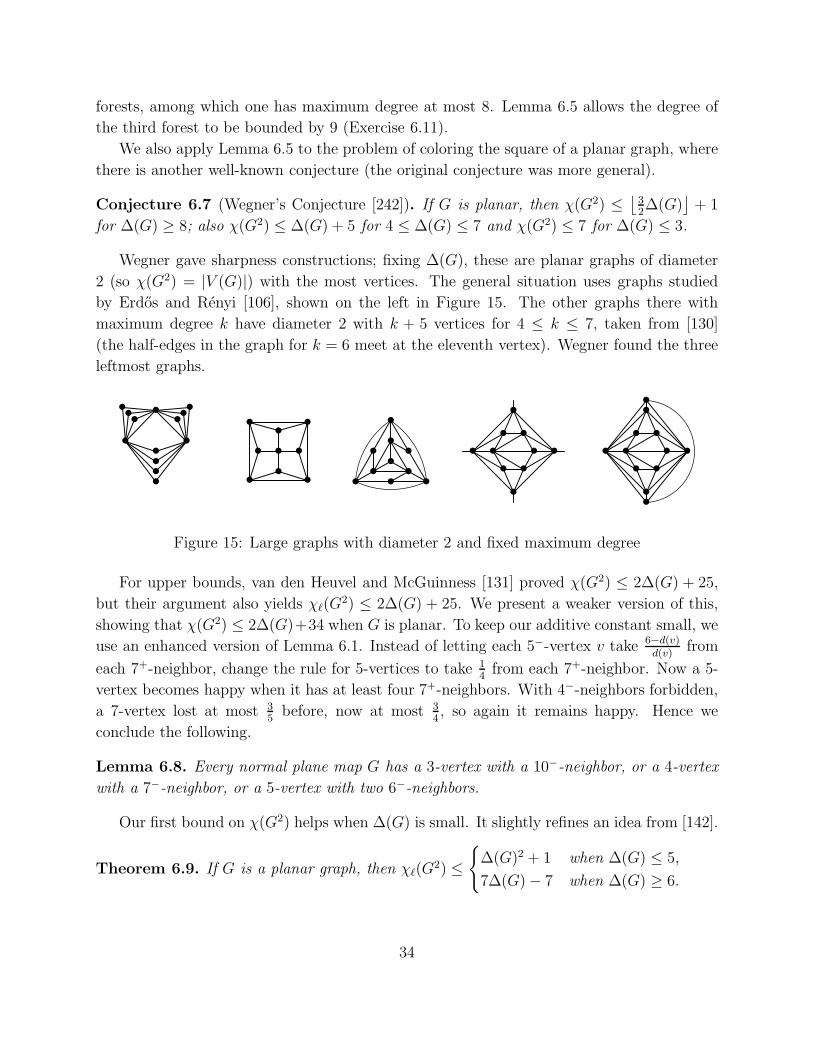
forests, among which one has maximum degree at most 8. Lemma 6.5 allows the degree of
the third forest to be bounded by 9 (Exercise 6.11).
We also apply Lemma 6.5 to the problem of coloring the square of a planar graph, where
there is another well-known conjecture (the original conjecture was more general).
Conjecture 6.7 (Wegner’s Conjecture [242]). If G is planar, then χ(G2) ≤⌊
32∆(G)
⌋
+ 1
for ∆(G) ≥ 8; also χ(G2) ≤ ∆(G) + 5 for 4 ≤ ∆(G) ≤ 7 and χ(G2) ≤ 7 for ∆(G) ≤ 3.
Wegner gave sharpness constructions; fixing ∆(G), these are planar graphs of diameter
2 (so χ(G2) = |V (G)|) with the most vertices. The general situation uses graphs studied
by Erdos and Renyi [106], shown on the left in Figure 15. The other graphs there with
maximum degree k have diameter 2 with k + 5 vertices for 4 ≤ k ≤ 7, taken from [130]
(the half-edges in the graph for k = 6 meet at the eleventh vertex). Wegner found the three
leftmost graphs.
•••• •••
• •
•••
•
•
••
• ••
•• • •
• ••••
•
•
••
••
•••••
•
•
•••
•••••
•
•
•
•
•
Figure 15: Large graphs with diameter 2 and fixed maximum degree
For upper bounds, van den Heuvel and McGuinness [131] proved χ(G2) ≤ 2∆(G) + 25,
but their argument also yields χℓ(G2) ≤ 2∆(G) + 25. We present a weaker version of this,
showing that χ(G2) ≤ 2∆(G)+34 when G is planar. To keep our additive constant small, we
use an enhanced version of Lemma 6.1. Instead of letting each 5−-vertex v take 6−d(v)d(v)
from
each 7+-neighbor, change the rule for 5-vertices to take 14from each 7+-neighbor. Now a 5-
vertex becomes happy when it has at least four 7+-neighbors. With 4−-neighbors forbidden,
a 7-vertex lost at most 35before, now at most 3
4, so again it remains happy. Hence we
conclude the following.
Lemma 6.8. Every normal plane map G has a 3-vertex with a 10−-neighbor, or a 4-vertex
with a 7−-neighbor, or a 5-vertex with two 6−-neighbors.
Our first bound on χ(G2) helps when ∆(G) is small. It slightly refines an idea from [142].
Theorem 6.9. If G is a planar graph, then χℓ(G2) ≤
∆(G)2 + 1 when ∆(G) ≤ 5,
7∆(G)− 7 when ∆(G) ≥ 6.
34
Proof. For ∆(G) ≤ 5, the claim is just the trivial upper bound from ∆(G2), so we may
assume ∆(G) ≥ 6.
Index the vertices from vn to v1 as follows. Having chosen vn, . . . , vi+1, let Gi = G −vn, . . . , vi+1. If δ(Gi) ≤ 3, then let vi be a vertex of minimum degree; otherwise let v be
a vertex as guaranteed by Lemma 6.8. Let Si = v1, . . . , vi. We choose colors for vertices
in the order v1, . . . , vn so that the coloring of Si satisfies all the constraints in the full graph
G2 from pairs of vertices in Si.
Let j = |N(vi)∩Si|; by the choice of the ordering, j ≤ 5. The other neighbors of vi occur
later and are not yet colored. However, vi must avoid the colors on the neighbors in Si of
these vertices; there may be up to 4(∆(G)− j) such colors. For u ∈ N(vi)∩Si, all neighbors
of u may lie in Si, so there may be as many as d(u) colors that vi must avoid due to u.
If j ≤ 3, then the number of colors vi must avoid is at most 4(∆(G)−j)+j∆(G). If j = 4,
then the bound is 7∆(G)−9, since vi has a 7−-neighbor in Si. If j = 5, then it is 7∆(G)−8,
since vi has two 6−-neighbors in Si. Hence always the bound is at most 7∆(G)− 8.
Using Lemma 6.5 instead of Lemma 6.8, a vertex with j earlier neighbors must avoid at
most 6∆(G) + 7j − 2 colors. Hence χℓ(G2) ≤ 6∆(G) + 33. We strengthen this bound.
Theorem 6.10. If G is a planar graph, then χℓ(G2) ≤ 2∆(G) + 34.
Proof. Theorem 6.9 provides upper bounds that are at most 2∆(G) + 34 when ∆(G) ≤ 8.
Hence we may assume ∆(G) ≥ 9.
Let G be a minimal counterexample, with list assignment L from which no such coloring
can be chosen. We will form G′ by contracting an edge of G incident to a 5−-vertex v,
viewed as absorbing v into the other endpoint u; the new vertex retains the list assigned to
u. All the constraints forcing vertices of G to have distinct colors are present also in G′, so
any proper coloring of the square of G′ can also be used on V (G′) in G. If ∆(G′) is small
enough, then the induction hypothesis applies to properly color the square of G′ from lists
of the desired size, and the task is only to show that few enough other vertices are within
distance 2 of v in G, leaving a color available for v to complete an L-coloring of G2.
If δ(G) ≤ 2, then let v be a vertex of minimum degree. The contracted vertex has degree
at most ∆(G). At most 2∆(G) vertices are within distance 2 of v, which leaves a color
available for v. Hence we may assume δ(G) ≥ 3, so Lemmas 6.8 and 6.5 apply.
Case 1: 9 ≤ ∆(G) ≤ 13. In this case we prove χℓ(G2) ≤ 52 ≤ 2∆(G) + 34. Let v
be a vertex as guaranteed by Lemma 6.8: a 3-vertex with a 10−-neighbor, a 4-vertex with
a 7−-neighbor, or a 5-vertex with two 6−-neighbors. The specified edge is the edge to be
contracted, and the degree of the new vertex is at most 11. Thus ∆(G′) ≤ 13, and the
induction hypothesis yields a proper L-coloring of the square of G′ from lists of size 52 (if
∆(G′) = 8, then χℓ(G′2) ≤ 2∆(G′) + 34 ≤ 52). The bound on the number of other vertices
35
within distance 2 of v is 2∆(G) + 10 for d(v) = 3, 3∆(G) + 7 for d(v) = 4, and 3∆(G) + 12
for d(v) = 5. Since ∆(G) ≤ 13, the value in each case is at most 51.
Case 2: ∆(G) ≥ 14. Let v be a vertex as guaranteed by Lemma 6.5; note that d(v) ≤ 5.
Since d(v) ≥ 3 and v has at most two 12+-neighbors, v has an 11−-neighbor; contract such
an edge. The contracted vertex has degree at most 14, so the induction hypothesis applies.
Also, the number of vertices within distance 2 of v in G is bounded by 2∆(G) + 33.
The improved upper bound of 2∆(G) + 25 in [131] uses a slightly stronger version of
Lemma 6.5 to improve the argument for large ∆(G) (see Exercise 6.13). Their main addi-
tional work was proving a second lemma specifically for graphs with small maximum degree.
Havet, van den Heuvel, McDiarmid, and Reed [127] proved for planar graphs that
χℓ(G2) ≤ (3
2+ o(1))∆(G) as ∆(G) → ∞, by probabilistic methods. Hence we also seek
bounds below 2∆(G) when ∆(G) is “small”. Borodin et al. [47] proved for planar graphs
that χℓ(G2) ≤ 59 when ∆(G) ≤ 20 and χℓ(G
2) ≤ max∆(G) + 39,⌈
95∆(G)
⌉
+ 1 when
∆(G) > 20. In particular, if ∆(G) ≥ 47, then χℓ(G2) ≤
⌈
95∆(G)
⌉
+ 1. More generally, they
proved that G2 is k-degenerate, where k = max∆(G) + 38,⌈
95∆(G)
⌉
. For the coloring
problem alone, Molloy and Salavatipour [178] proved χ(G2) ≤ 53∆(G) + 78 for all planar G.
For results in terms of mad(G) (without planarity), see the exercises in Section 3.
We have noted that many results for planar graphs with girth at least g extend to the
family of graphs G with mad(G) < 2gg−2
(especially when the proof uses vertex charging). In
some cases, planarity permits a stronger result, meaning that obtaining the same conclusion
using only a bound on mad(G) requires mad(G) < b for some b smaller than 2gg−2
.
For example, consider a special case of Exercise 3.3: every graph G with mad(G) < 83and
δ(G) ≥ 2 has a 2-vertex with a 3−-neighbor. This applies to planar graphs with girth at least
8. The result in terms of mad(G) is sharp, since subdividing every edge of a 4-regular graph
yields a graph G with mad(G) = 83having no such vertex. However, the conclusion holds
for planar graphs with girth 7, which allow mad(G) to be larger, so in this case planarity
is needed to obtain the best result. The argument we present illustrates typical difficulties
that may arise when discovering discharging arguments.
Lemma 6.11. Every planar graph G with girth at least 7 and δ(G) ≥ 2 has a 2-vertex with
a neighbor of degree at most 3.
Proof. Assume that G has no such configuration. Use face charging, giving each vertex v
initial charge 2d(v) − 6 and each face f initial charge ℓ(f) − 6. The total charge is −12.
Since g has girth at least 7, the only objects with negative initial charge are 2-vertices. Let
each 2-vertex take 12from each neighbor and each incident face. To complete the proof, we
check that all vertices and faces end with nonnegative charge.
The discharging rule ensures that 2-vertices end with charge 0. Since 3-vertices have no
2-neighbors, their charge remains 0. For j ≥ 4, a j-vertex may lose 12along each edge and
36
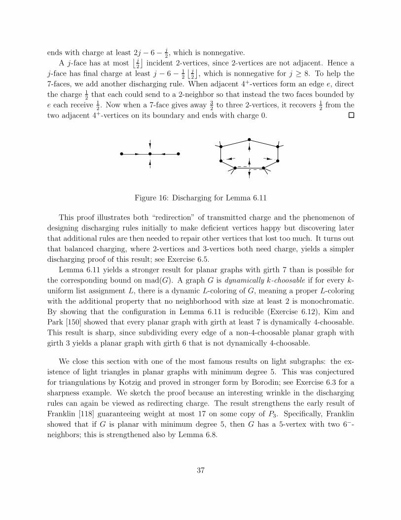
ends with charge at least 2j − 6− j2, which is nonnegative.
A j-face has at most⌊
j2
⌋
incident 2-vertices, since 2-vertices are not adjacent. Hence a
j-face has final charge at least j − 6 − 12
⌊
j2
⌋
, which is nonnegative for j ≥ 8. To help the
7-faces, we add another discharging rule. When adjacent 4+-vertices form an edge e, direct
the charge 12that each could send to a 2-neighbor so that instead the two faces bounded by
e each receive 12. Now when a 7-face gives away 3
2to three 2-vertices, it recovers 1
2from the
two adjacent 4+-vertices on its boundary and ends with charge 0.
••
• •••
••
• •
Figure 16: Discharging for Lemma 6.11
This proof illustrates both “redirection” of transmitted charge and the phenomenon of
designing discharging rules initially to make deficient vertices happy but discovering later
that additional rules are then needed to repair other vertices that lost too much. It turns out
that balanced charging, where 2-vertices and 3-vertices both need charge, yields a simpler
discharging proof of this result; see Exercise 6.5.
Lemma 6.11 yields a stronger result for planar graphs with girth 7 than is possible for
the corresponding bound on mad(G). A graph G is dynamically k-choosable if for every k-
uniform list assignment L, there is a dynamic L-coloring of G, meaning a proper L-coloring
with the additional property that no neighborhood with size at least 2 is monochromatic.
By showing that the configuration in Lemma 6.11 is reducible (Exercise 6.12), Kim and
Park [150] showed that every planar graph with girth at least 7 is dynamically 4-choosable.
This result is sharp, since subdividing every edge of a non-4-choosable planar graph with
girth 3 yields a planar graph with girth 6 that is not dynamically 4-choosable.
We close this section with one of the most famous results on light subgraphs: the ex-
istence of light triangles in planar graphs with minimum degree 5. This was conjectured
for triangulations by Kotzig and proved in stronger form by Borodin; see Exercise 6.3 for a
sharpness example. We sketch the proof because an interesting wrinkle in the discharging
rules can again be viewed as redirecting charge. The result strengthens the early result of
Franklin [118] guaranteeing weight at most 17 on some copy of P3. Specifically, Franklin
showed that if G is planar with minimum degree 5, then G has a 5-vertex with two 6−-
neighbors; this is strengthened also by Lemma 6.8.
37
Theorem 6.12 (Borodin [40]). If G is a simple plane graph with δ(G) ≥ 5, then G has a
3-face with weight at most 17, and the bound is sharp.
Proof. (sketch) For sharpness, add a vertex in each face of the dodecahedron joined to the
vertices of that face. The new vertices have degree 5, and the old ones now have degree 6.
Every face has one new vertex and two old vertices for total weight 17.
To prove the bound, consider an edge-maximal counterexample G. Every vertex on a
4+-face has degree 5, since adding a triangular chord at a 6+-vertex would create only heavy
3-faces, producing a counterexample containing G.
Suppose there is no light triangle and use vertex charging, with charge d(v)− 6 on each
vertex v and 2l(f)− 6 on each face f . Move charge via the following rules:
(R1) Each 4+-face gives 12to each incident vertex.
(R2) Each 7-vertex gives 13to each 5-neighbor.
(R3) Each 8+-vertex gives 14through each incident 3-face to its 5-neighbors on that face,
split equally if there are two such neighbors.
It suffices to show that final charges are nonnegative. The discharging rules are chosen
so that 4+-faces and 7+-vertices do not give away too much charge. (Maximality of the
counterexample puts a 7-vertex on seven triangles, and absence of light triangles then restricts
a 7-vertex to have at most three 5-neighbors).
Hence the task is to prove that a 5-vertex v gains charge 1. When all incident faces are
triangles, avoiding light triangles restricts v to have at most two 5-neighbors. It also forces
the other neighbors to be 8+-vertices when v has two 5-neighbors. In this and the remaining
cases (such as when v lies on a 4+-face), it is easy to check that v receives enough charge.
In each discharging rule in Theorem 6.12, the charge given away is the most that object
can afford to lose. Only 5-vertices need to gain charge. Hence it would be natural to have
8+-vertices give 14to each 5-neighbor. However, this would give only 3
4to a 5-vertex having
two 5-neighbors and three 8-neighbors. The 5-vertex needs to get more when it has two
8-neighbors on a single triangle. Guiding the charge from 8+-neighbors through the incident
triangles is a way to arrange that.
Exercise 6.1. Construct planar graphs to show that the bounds in Lemma 6.1 are sharp. That is,none of the values 10, 7, 6 can be reduced in the statement that normal plane maps have a 3-vertexwith a 10−-neighbor, a 4-vertex with a 7−-neighbor, or a 5-vertex with a 6−-neighbor.
Exercise 6.2. Prove that planarity is needed in Lemma 6.1 by showing that a graph G withmad(G) < 6 and δ(G) = 5 need not have a 5-vertex with any 6−-neighbor.
Exercise 6.3. Prove that requiring minimum degree 5 in Theorem 6.12 is necessary, by constructingfor each k ∈ N a planar graph with minimum degree 4 having no triangle with weight at most k.
38
Exercise 6.4. The argument in Remark 2.3 with ℓ = 2 shows that 125 is the largest ρ such that
mad(G) < ρ guarantees adjacent 2-vertices in G. Note that mad(G) < 125 when G is planar
with girth at least 12. Restriction to planar graphs permits a stronger result: Prove that planargraphs with girth at least 11 have adjacent 2-vertices, and provide a construction to show that theconclusion fails for some planar graph with girth 10.
Exercise 6.5. Use balanced charging to prove that every planar graph with girth at least 7 andminimum degree at least 2 has a 2-vertex adjacent to a 3−-vertex. Prove that the conclusion doesnot always hold when mad(G) < 14
5 (thus planarity is needed). Show that the conclusion does nothold for all planar graphs with girth 6.
Exercise 6.6. Planar graphs with girth at least 6 satisfy mad(G) < 3, so by Exercise 2.1 eachsuch graph has a 2-vertex with a 5−-neighbor. Show that this is sharp even for planar graphs byconstructing a planar graph with girth 6 having no edge of weight at most 6.
Exercise 6.7. Determine whether a planar graph with girth at least 4 and minimum degree 3must have a 3-vertex with a 4−-neighbor. Construct a planar graph Gk with girth 4 and minimumdegree 3 in which the distance between 3-vertices is at least k. Construct a planar graph Hk withminimum degree 5 in which the distance between 5-vertices is at least k.
Exercise 6.8. Let G be a graph with δ(G) ≥ 3 and mad(G) < 103 . Prove that G has a 3-vertex
whose neighbors have degree-sum at most 10. Prove that this result is sharp even in the family ofplanar graphs with girth at least 5 by constructing such a graph in which no 3-vertex has three3-neighbors. (Comment: G. Tardos constructed such a graph with 98 vertices.)
Exercise 6.9. (Borodin [44]) Prove that every planar graph with minimum degree 5 contains two 3-faces sharing an edge with weight at most 11. Show that this configuration is reducible for χ′′′(G) ≤12. (Hint: Use vertex charging, with 5-vertices taking 1
2 from incident 4+-faces and the remainingneeded charge from 7+-neighbors. Comments: Borodin proved a stronger structural conclusion andused it in his proof that χ′′′(G) ≤ ∆(G) + 4 when ∆(G) ≥ 7; the proof of the statement here issimpler. Note also the similarity between the configurations here and in Exercise 5.4).
Exercise 6.10. (Cranston) Give a short proof that χ′′′(G) ≤ ∆(G) + 4 when G is a planar graphwith ∆(G) ≥ 7 by using the technique in the proof of Theorem 4.7, relying on Theorem 6.2 insteadof the Four Color Theorem.
Exercise 6.11. Prove inductively that every planar graph decomposes into three forests. (Hint:Reduce to triangulations, and then apply the induction hypothesis to a smaller graph obtained bydeleting a light vertex and triangulating the resulting face. There are a number of cases when thedeleted vertex has degree 5, depending on the usage of the two added edges.) Use Lemma 6.5 andmore detailed analysis to prove that the third forests can be guaranteed to have maximum degreeat most 9. (Comment: The second part of this exercise is long. See Balogh et al. [22] for maximumdegree at most 8.)
Exercise 6.12. (Kim and Park [150]) Prove that among the planar graphs with girth at least7, a minimal graph that is not dynamically 4-choosable cannot contain a 2-vertex with a 3−-neighbor. (Comment: With Lemma 6.11, this proves that every planar graph with girth at least7 is dynamically 4-choosable. Note that mad(G) < 14
5 when G is planar with girth at least 7, butmad(G) < 14
5 is not sufficient for dynamic 4-choosability.)
39
Exercise 6.13. van den Heuvel and McGuinness [131] refined Lemma 6.5 to state that a planargraph G with δ(G) ≥ 3 has a 5−-vertex v with at most two 12+-neighbors such that v has a 7−-neighbor if d(v) ∈ 4, 5, and v has an additional 6−-neighbor if d(v) = 5 (see Exercise 7.14). Usethis to prove that χ(G2) ≤ 2∆(G) + 25 when ∆(G) ≥ 12.
7 Stronger and Weaker Colorings
In this section, we consider both restricted and relaxed versions of proper coloring. As a
relaxation, we study “improper” coloring, where the subgraph induced by a color class has
maximum degree at most d; proper coloring is the case d = 0. First we study restricted
versions of coloring. For example, the union of two color classes in a proper coloring induces
a bipartite graph; we may further restrict the bipartite graphs allowed to arise.
7.1 Acyclic Coloring
An acyclic coloring of a graph G is a proper coloring in which the union of any two color
classes induces a forest. Equivalently, no cycle is 2-colored. Let a(G) denote the minimum
number of colors in an acyclic coloring of G.
Grunbaum [123] conjectured that planar graphs are acyclically 5-colorable, observed that
the graph of the octahedron is not acyclically 4-colorable, and proved that planar graphs are
acyclically 9-colorable. Improved upper bounds of 8 [176], 7 [7], and 6 [151] culminated in
the result of Borodin [36] that a(G) ≤ 5 when G is planar. The bound is sharp, even among
bipartite planar graphs [153] (Exercise 7.2). Borodin’s proof used discharging with some 450
reducible configurations but no computers.
We present the earlier result by Albertson and Berman [7] that planar graphs are acycli-
cally 7-colorable; it has several interesting features. In the discharging, the strictly negative
charge from Euler’s Formula is used to keep the forced configurations away from the un-
bounded face. In the reducibility, the smaller graphs used in coloring G are modifications of
subgraphs of G. Our proof simplifies some aspects of the original proof.
A near-triangulation is a plane graph in which every bounded face is a triangle. A vertex
not incident to the unbounded face is an internal vertex. Our modification of Lemma 6.1 is
closely tailored to the reducibility arguments in Theorem 7.2.
Lemma 7.1. Let G be a near-triangulation with δ(G) ≥ 3. If the outer face has length 4
and G has at least two internal vertices, then G contains an internal 3-vertex, or an internal
4-vertex or 5-vertex with an internal 6−-neighbor, or an internal 7-vertex with two internal
4-neighbors. If the outer face has length 3, then again G contains one of these configurations,
but without the restriction to internal vertices.
Proof. For triangulations, consider the proof of Lemma 6.1. If we change the forbidden
configuration at a 7-vertex to require two 4-neighbors (so 7-vertices with one 4-neighbor
40
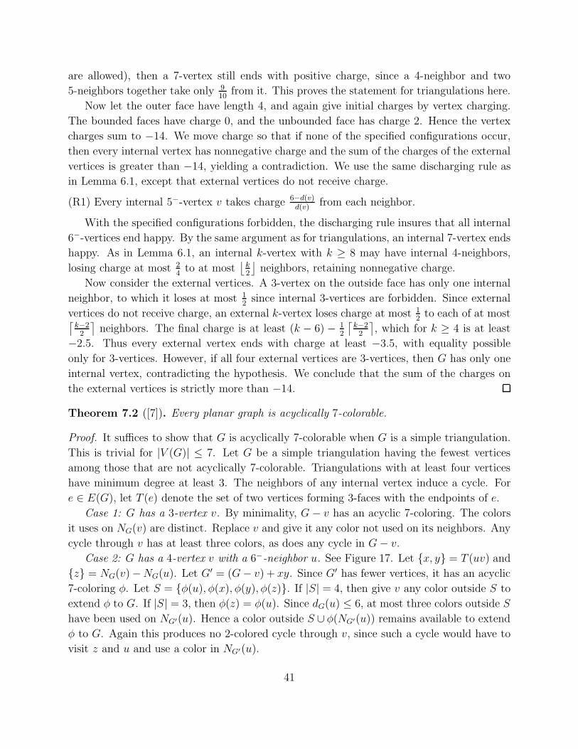
are allowed), then a 7-vertex still ends with positive charge, since a 4-neighbor and two
5-neighbors together take only 910
from it. This proves the statement for triangulations here.
Now let the outer face have length 4, and again give initial charges by vertex charging.
The bounded faces have charge 0, and the unbounded face has charge 2. Hence the vertex
charges sum to −14. We move charge so that if none of the specified configurations occur,
then every internal vertex has nonnegative charge and the sum of the charges of the external
vertices is greater than −14, yielding a contradiction. We use the same discharging rule as
in Lemma 6.1, except that external vertices do not receive charge.
(R1) Every internal 5−-vertex v takes charge 6−d(v)d(v)
from each neighbor.
With the specified configurations forbidden, the discharging rule insures that all internal
6−-vertices end happy. By the same argument as for triangulations, an internal 7-vertex ends
happy. As in Lemma 6.1, an internal k-vertex with k ≥ 8 may have internal 4-neighbors,
losing charge at most 24to at most
⌊
k2
⌋
neighbors, retaining nonnegative charge.
Now consider the external vertices. A 3-vertex on the outside face has only one internal
neighbor, to which it loses at most 12since internal 3-vertices are forbidden. Since external
vertices do not receive charge, an external k-vertex loses charge at most 12to each of at most
⌈
k−22
⌉
neighbors. The final charge is at least (k − 6) − 12
⌈
k−22
⌉
, which for k ≥ 4 is at least
−2.5. Thus every external vertex ends with charge at least −3.5, with equality possible
only for 3-vertices. However, if all four external vertices are 3-vertices, then G has only one
internal vertex, contradicting the hypothesis. We conclude that the sum of the charges on
the external vertices is strictly more than −14.
Theorem 7.2 ([7]). Every planar graph is acyclically 7-colorable.
Proof. It suffices to show that G is acyclically 7-colorable when G is a simple triangulation.
This is trivial for |V (G)| ≤ 7. Let G be a simple triangulation having the fewest vertices
among those that are not acyclically 7-colorable. Triangulations with at least four vertices
have minimum degree at least 3. The neighbors of any internal vertex induce a cycle. For
e ∈ E(G), let T (e) denote the set of two vertices forming 3-faces with the endpoints of e.
Case 1: G has a 3-vertex v. By minimality, G− v has an acyclic 7-coloring. The colors
it uses on NG(v) are distinct. Replace v and give it any color not used on its neighbors. Any
cycle through v has at least three colors, as does any cycle in G− v.
Case 2: G has a 4-vertex v with a 6−-neighbor u. See Figure 17. Let x, y = T (uv) and
z = NG(v)−NG(u). Let G′ = (G− v) + xy. Since G′ has fewer vertices, it has an acyclic
7-coloring φ. Let S = φ(u), φ(x), φ(y), φ(z). If |S| = 4, then give v any color outside S to
extend φ to G. If |S| = 3, then φ(z) = φ(u). Since dG(u) ≤ 6, at most three colors outside S
have been used on NG′(u). Hence a color outside S ∪ φ(NG′(u)) remains available to extend
φ to G. Again this produces no 2-colored cycle through v, since such a cycle would have to
visit z and u and use a color in NG′(u).
41
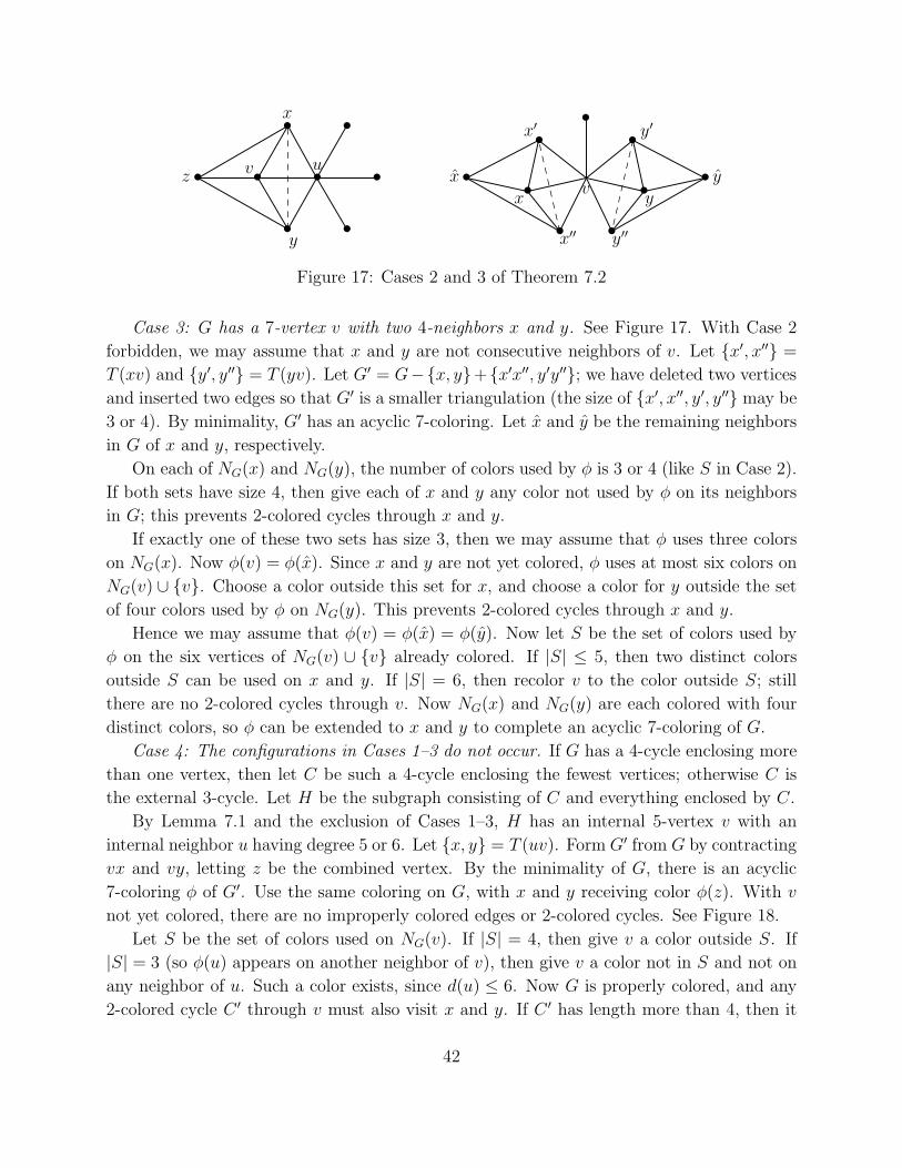
•
•
•
••
•
•
•
y
x
uvz
••
•
••
•
•
••y
vx
y′
y′′
y
x′
x′′
x
Figure 17: Cases 2 and 3 of Theorem 7.2
Case 3: G has a 7-vertex v with two 4-neighbors x and y. See Figure 17. With Case 2
forbidden, we may assume that x and y are not consecutive neighbors of v. Let x′, x′′ =
T (xv) and y′, y′′ = T (yv). Let G′ = G−x, y+x′x′′, y′y′′; we have deleted two vertices
and inserted two edges so that G′ is a smaller triangulation (the size of x′, x′′, y′, y′′ may be
3 or 4). By minimality, G′ has an acyclic 7-coloring. Let x and y be the remaining neighbors
in G of x and y, respectively.
On each of NG(x) and NG(y), the number of colors used by φ is 3 or 4 (like S in Case 2).
If both sets have size 4, then give each of x and y any color not used by φ on its neighbors
in G; this prevents 2-colored cycles through x and y.
If exactly one of these two sets has size 3, then we may assume that φ uses three colors
on NG(x). Now φ(v) = φ(x). Since x and y are not yet colored, φ uses at most six colors on
NG(v) ∪ v. Choose a color outside this set for x, and choose a color for y outside the set
of four colors used by φ on NG(y). This prevents 2-colored cycles through x and y.
Hence we may assume that φ(v) = φ(x) = φ(y). Now let S be the set of colors used by
φ on the six vertices of NG(v) ∪ v already colored. If |S| ≤ 5, then two distinct colors
outside S can be used on x and y. If |S| = 6, then recolor v to the color outside S; still
there are no 2-colored cycles through v. Now NG(x) and NG(y) are each colored with four
distinct colors, so φ can be extended to x and y to complete an acyclic 7-coloring of G.
Case 4: The configurations in Cases 1–3 do not occur. If G has a 4-cycle enclosing more
than one vertex, then let C be such a 4-cycle enclosing the fewest vertices; otherwise C is
the external 3-cycle. Let H be the subgraph consisting of C and everything enclosed by C.
By Lemma 7.1 and the exclusion of Cases 1–3, H has an internal 5-vertex v with an
internal neighbor u having degree 5 or 6. Let x, y = T (uv). Form G′ from G by contracting
vx and vy, letting z be the combined vertex. By the minimality of G, there is an acyclic
7-coloring φ of G′. Use the same coloring on G, with x and y receiving color φ(z). With v
not yet colored, there are no improperly colored edges or 2-colored cycles. See Figure 18.
Let S be the set of colors used on NG(v). If |S| = 4, then give v a color outside S. If
|S| = 3 (so φ(u) appears on another neighbor of v), then give v a color not in S and not on
any neighbor of u. Such a color exists, since d(u) ≤ 6. Now G is properly colored, and any
2-colored cycle C ′ through v must also visit x and y. If C ′ has length more than 4, then it
42
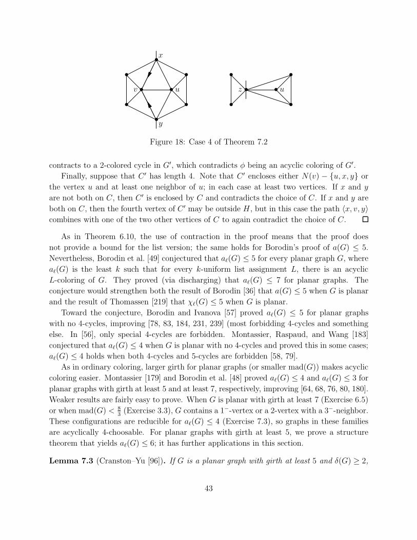
••
•••
••
•
y
uv
••
••
••
x
z u
Figure 18: Case 4 of Theorem 7.2
contracts to a 2-colored cycle in G′, which contradicts φ being an acyclic coloring of G′.
Finally, suppose that C ′ has length 4. Note that C ′ encloses either N(v) − u, x, y or
the vertex u and at least one neighbor of u; in each case at least two vertices. If x and y
are not both on C, then C ′ is enclosed by C and contradicts the choice of C. If x and y are
both on C, then the fourth vertex of C ′ may be outside H , but in this case the path 〈x, v, y〉combines with one of the two other vertices of C to again contradict the choice of C.
As in Theorem 6.10, the use of contraction in the proof means that the proof does
not provide a bound for the list version; the same holds for Borodin’s proof of a(G) ≤ 5.
Nevertheless, Borodin et al. [49] conjectured that aℓ(G) ≤ 5 for every planar graph G, where
aℓ(G) is the least k such that for every k-uniform list assignment L, there is an acyclic
L-coloring of G. They proved (via discharging) that aℓ(G) ≤ 7 for planar graphs. The
conjecture would strengthen both the result of Borodin [36] that a(G) ≤ 5 when G is planar
and the result of Thomassen [219] that χℓ(G) ≤ 5 when G is planar.
Toward the conjecture, Borodin and Ivanova [57] proved aℓ(G) ≤ 5 for planar graphs
with no 4-cycles, improving [78, 83, 184, 231, 239] (most forbidding 4-cycles and something
else. In [56], only special 4-cycles are forbidden. Montassier, Raspaud, and Wang [183]
conjectured that aℓ(G) ≤ 4 when G is planar with no 4-cycles and proved this in some cases;
aℓ(G) ≤ 4 holds when both 4-cycles and 5-cycles are forbidden [58, 79].
As in ordinary coloring, larger girth for planar graphs (or smaller mad(G)) makes acyclic
coloring easier. Montassier [179] and Borodin et al. [48] proved aℓ(G) ≤ 4 and aℓ(G) ≤ 3 for
planar graphs with girth at least 5 and at least 7, respectively, improving [64, 68, 76, 80, 180].
Weaker results are fairly easy to prove. When G is planar with girth at least 7 (Exercise 6.5)
or when mad(G) < 83(Exercise 3.3), G contains a 1−-vertex or a 2-vertex with a 3−-neighbor.
These configurations are reducible for aℓ(G) ≤ 4 (Exercise 7.3), so graphs in these families
are acyclically 4-choosable. For planar graphs with girth at least 5, we prove a structure
theorem that yields aℓ(G) ≤ 6; it has further applications in this section.
Lemma 7.3 (Cranston–Yu [96]). If G is a planar graph with girth at least 5 and δ(G) ≥ 2,
43
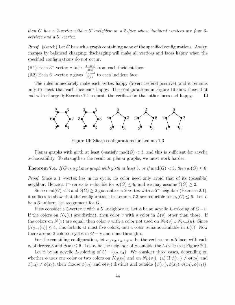
then G has a 2-vertex with a 5−-neighbor or a 5-face whose incident vertices are four 3-
vertices and a 5−-vertex.
Proof. (sketch) Let G be such a graph containing none of the specified configurations. Assign
charges by balanced charging; discharging will make all vertices and faces happy when the
specified configurations do not occur.
(R1) Each 3−-vertex v takes 4−d(v)d(v)
from each incident face.
(R2) Each 6+-vertex v gives d(v)−4d(v)
to each incident face.
The rules immediately make each vertex happy (5-vertices end positive), and it remains
only to check that each face ends happy. The configurations in Figure 19 show faces that
end with charge 0; Exercise 7.1 requests the verification that other faces end happy.
••
•••• 6
2
62
6
2 ••
•••• 3
3
33
3
3 ••
••
•6
3
33
3•
•
••
•2
6
33
6•
•
••
•6
2
66
2
Figure 19: Sharp configurations for Lemma 7.3
Planar graphs with girth at least 6 satisfy mad(G) < 3, and this is sufficient for acyclic
6-choosability. To strengthen the result on planar graphs, we must work harder.
Theorem 7.4. If G is a planar graph with girth at least 5, or if mad(G) < 3, then aℓ(G) ≤ 6.
Proof. Since a 1−-vertex lies in no cycle, its color need only avoid that of its (possible)
neighbor. Hence a 1−-vertex is reducible for aℓ(G) ≤ 6, and we may assume δ(G) ≥ 2.
Since mad(G) < 3 and δ(G) ≥ 2 guarantees a 2-vertex with a 5−-neighbor (Exercise 2.1),
it suffices to show that the configurations in Lemma 7.3 are reducible for aℓ(G) ≤ 6. Let L
be a 6-uniform list assignment for G.
First consider a 2-vertex v with a 5−-neighbor u. Let φ be an acyclic L-coloring of G−v.
If the colors on NG(v) are distinct, then color v with a color in L(v) other than those. If
the colors on N(v) are equal, then color v with a color not used on NG(v) ∪NG−v(u). Since
|NG−v(u)| ≤ 4, this forbids at most five colors, and a color remains available in L(v). Now
there are no 2-colored cycles in G− v and none through v.
For the remaining configuration, let v1, v2, v3, v4, w be the vertices on a 5-face, with each
vi of degree 3 and d(w) ≤ 5. Let xi be the neighbor of vi outside the 5-cycle (see Figure 20).
Let φ be an acyclic L-coloring of G − v2, v3. We consider three cases, depending on
whether φ uses one color or two colors on NG(v2) and on NG(v3). (a) If φ(v1) 6= φ(x2) and
φ(v4) 6= φ(x3), then choose φ(v2) and φ(v3) distinct and outside φ(v1), φ(x2), φ(x3), φ(v4).
44
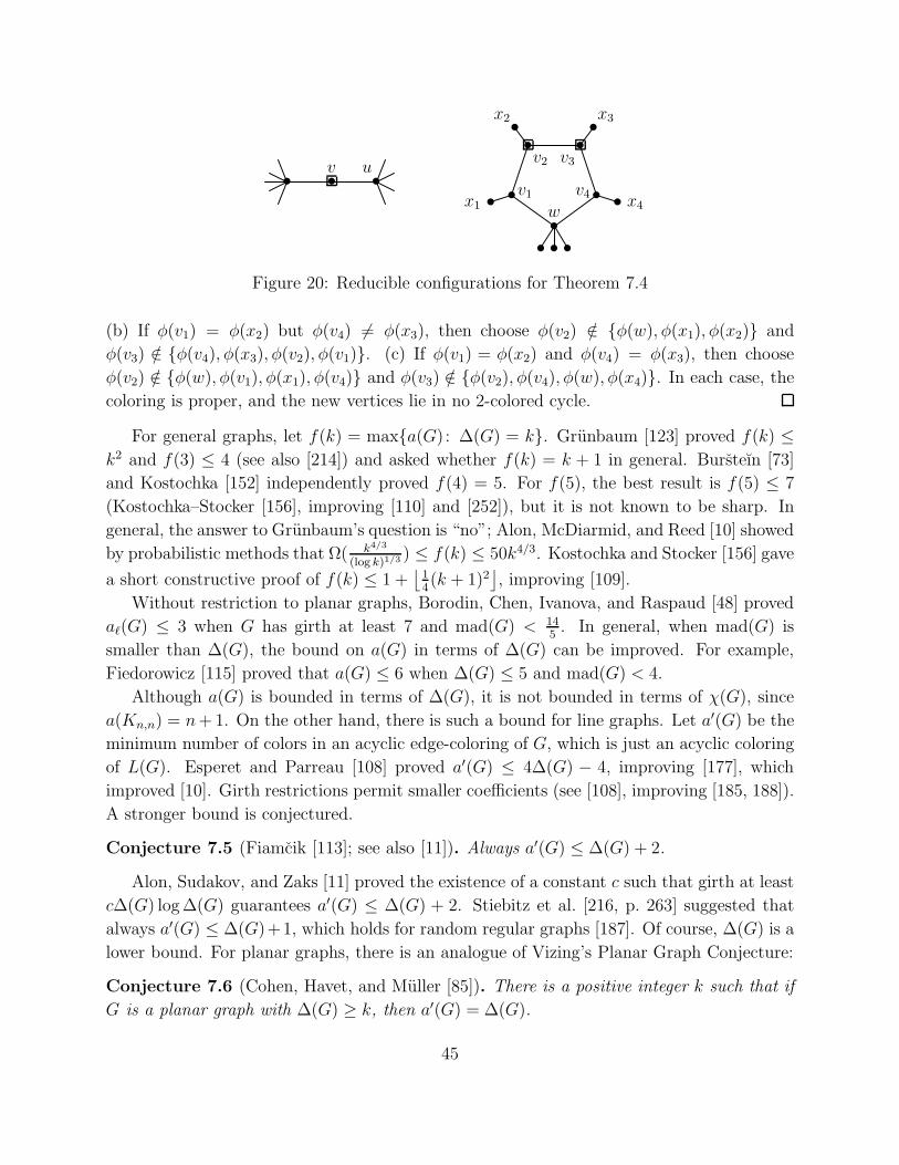
• • •v u
••
• •
•w
v1
v2 v3
v4
•
•
• •
•
• •
x1
x2 x3
x4
Figure 20: Reducible configurations for Theorem 7.4
(b) If φ(v1) = φ(x2) but φ(v4) 6= φ(x3), then choose φ(v2) /∈ φ(w), φ(x1), φ(x2) and
φ(v3) /∈ φ(v4), φ(x3), φ(v2), φ(v1). (c) If φ(v1) = φ(x2) and φ(v4) = φ(x3), then choose
φ(v2) /∈ φ(w), φ(v1), φ(x1), φ(v4) and φ(v3) /∈ φ(v2), φ(v4), φ(w), φ(x4). In each case, the
coloring is proper, and the new vertices lie in no 2-colored cycle.
For general graphs, let f(k) = maxa(G) : ∆(G) = k. Grunbaum [123] proved f(k) ≤k2 and f(3) ≤ 4 (see also [214]) and asked whether f(k) = k + 1 in general. Bursteın [73]
and Kostochka [152] independently proved f(4) = 5. For f(5), the best result is f(5) ≤ 7
(Kostochka–Stocker [156], improving [110] and [252]), but it is not known to be sharp. In
general, the answer to Grunbaum’s question is “no”; Alon, McDiarmid, and Reed [10] showed
by probabilistic methods that Ω( k4/3
(log k)1/3) ≤ f(k) ≤ 50k4/3. Kostochka and Stocker [156] gave
a short constructive proof of f(k) ≤ 1 +⌊
14(k + 1)2
⌋
, improving [109].
Without restriction to planar graphs, Borodin, Chen, Ivanova, and Raspaud [48] proved
aℓ(G) ≤ 3 when G has girth at least 7 and mad(G) < 145. In general, when mad(G) is
smaller than ∆(G), the bound on a(G) in terms of ∆(G) can be improved. For example,
Fiedorowicz [115] proved that a(G) ≤ 6 when ∆(G) ≤ 5 and mad(G) < 4.
Although a(G) is bounded in terms of ∆(G), it is not bounded in terms of χ(G), since
a(Kn,n) = n+1. On the other hand, there is such a bound for line graphs. Let a′(G) be the
minimum number of colors in an acyclic edge-coloring of G, which is just an acyclic coloring
of L(G). Esperet and Parreau [108] proved a′(G) ≤ 4∆(G) − 4, improving [177], which
improved [10]. Girth restrictions permit smaller coefficients (see [108], improving [185, 188]).
A stronger bound is conjectured.
Conjecture 7.5 (Fiamcik [113]; see also [11]). Always a′(G) ≤ ∆(G) + 2.
Alon, Sudakov, and Zaks [11] proved the existence of a constant c such that girth at least
c∆(G) log∆(G) guarantees a′(G) ≤ ∆(G) + 2. Stiebitz et al. [216, p. 263] suggested that
always a′(G) ≤ ∆(G)+1, which holds for random regular graphs [187]. Of course, ∆(G) is a
lower bound. For planar graphs, there is an analogue of Vizing’s Planar Graph Conjecture:
Conjecture 7.6 (Cohen, Havet, and Muller [85]). There is a positive integer k such that if
G is a planar graph with ∆(G) ≥ k, then a′(G) = ∆(G).
45
The existence of such k was proved in [85] for the family of planar graphs with mad(G) ≤4 − ǫ, for any fixed ǫ. When mad(G) < 10
3, Basavaraju et al. [28] proved that ∆(G) ≥ 19
suffices. Several papers have provided pairs (k, g) such that a′(G) = ∆(G) for all planar
graphs with ∆(G) ≥ k and girth at least g.
Lemma 6.5 easily yields a′(G) ≤ 2∆(G) + 33 when G is planar (Exercise 7.5). Wang et
al. [234] proved that ∆(G) + 7 colors suffice for planar graphs, improving upper bounds of
2∆(G) + 29 [117], max2∆(G)− 2,∆(G) + 22 [136], ∆(G) + 25 [85], ∆(G) + 12 [28], and
∆(G)+10 [124]. The bound improves to ∆(G)+3 for girth at least 4 [27] (improving [117]),
to ∆(G)+ 2 for girth at least 5 [70, 136], and to ∆(G) + 1 for girth at least 6 [70, 253] or for
girth 5 when ∆(G) ≥ 11 [253]).
Bounds on a′(G) have been given for planar graphs under various sets of forbidden cycle
lengths; one goal is to prove Conjecture 7.5 under the weakest possible restrictions. For
example, a′(G) ≤ ∆(G) + 2 for planar graphs with no 5-cycles [208], with no 4-cycles [235],
and with no 3-cycles [209]; furthermore, the bound still holds when no 3-cycle is adjacent to
a 4-cycle [236] and when no 3-cycle is adjacent to a 6-cycle [238].
Beyond planar graphs, Fiedorowicz [114] proved for integer t that a′(G) ≤ (t−1)∆(G)+
2t3 − 3t + 2 when mad(G) < 2t. In terms of the maximum degree only, a′(G) ≤ 4 when
∆(G) = 3 except for K4 and K3,3 (in [24] for δ(G) < 3 and in [12] for 3-regular graphs,
improving [214]). If ∆(G) ≤ 4, then a′(G) ≤ 6 ([25] for δ(G) < 4 and [237] for 4-regular.
Also, a′(G) = ∆(G) when G is obtained from any other graph by subdividing each edge [116].
Finally, Lai and Lih [166] extended many of these results to the acyclic edge-choosability
a′ℓ(G), which is the minimum k such that an acyclic edge-coloring can be chosen from any
k-uniform assignment on the edges. For example, a′ℓ(G) ≤ ∆(G) + 1 for outerplanar graphs
and for non-regular graphs with ∆(G) = 3 (the bound is 5 for 3-regular graphs, and it is
∆(G) for outerplanar graphs with ∆(G) ≥ 5 [210]). In [165], they observed that many of the
bounds on a′(G) for planar graphs with forbidden cycle lengths hold also in the list context;
also, mad(G) < 4 implies a′ℓ(G) ≤ ∆(G) + 5 and mad(G) < 3 implies a′ℓ(G) ≤ ∆(G) + 1.
Extending Conjecture 7.5, they posed the following conjectures:
Conjecture 7.7 (Lai and Lih [166]). Every graph G satisfies a′ℓ(G) = a′(G). Every graph
G satisfies a′ℓ(G) ≤ ∆(G) + 2.
Exercise 7.1. Complete the proof of Lemma 7.3.
Exercise 7.2. (Grunbaum [123], Kostochka–Mel’nikov [153]) Prove that the two graphs in Fig-ure 21 are not acylically 4-colorable. The half-edges leaving the figure on the right lead to anadditional vertex having the same neighborhood as the central vertex.
Exercise 7.3. Prove that a 2-vertex with a 3−-neighbor is reducible for acyclic 4-choosability.
46
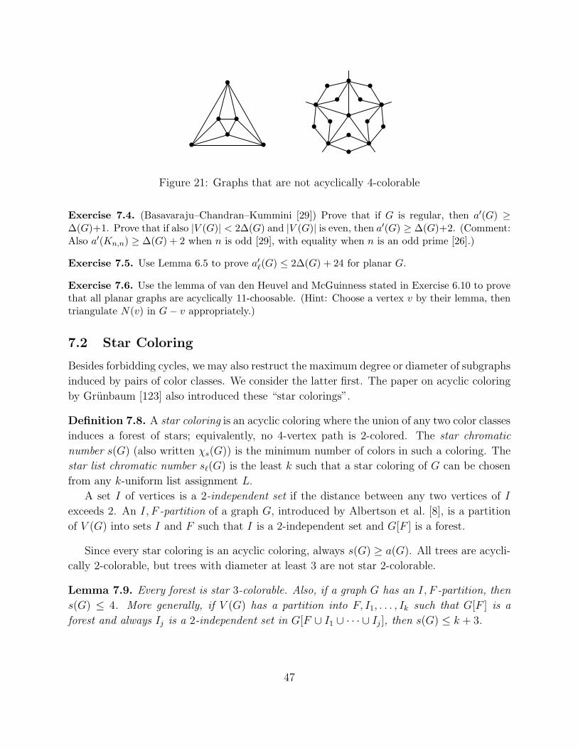
•
•••
• •
•
•
••
••
••
• •••
••
••
Figure 21: Graphs that are not acyclically 4-colorable
Exercise 7.4. (Basavaraju–Chandran–Kummini [29]) Prove that if G is regular, then a′(G) ≥∆(G)+1. Prove that if also |V (G)| < 2∆(G) and |V (G)| is even, then a′(G) ≥ ∆(G)+2. (Comment:Also a′(Kn,n) ≥ ∆(G) + 2 when n is odd [29], with equality when n is an odd prime [26].)
Exercise 7.5. Use Lemma 6.5 to prove a′ℓ(G) ≤ 2∆(G) + 24 for planar G.
Exercise 7.6. Use the lemma of van den Heuvel and McGuinness stated in Exercise 6.10 to provethat all planar graphs are acyclically 11-choosable. (Hint: Choose a vertex v by their lemma, thentriangulate N(v) in G− v appropriately.)
7.2 Star Coloring
Besides forbidding cycles, we may also restruct the maximum degree or diameter of subgraphs
induced by pairs of color classes. We consider the latter first. The paper on acyclic coloring
by Grunbaum [123] also introduced these “star colorings”.
Definition 7.8. A star coloring is an acyclic coloring where the union of any two color classes
induces a forest of stars; equivalently, no 4-vertex path is 2-colored. The star chromatic
number s(G) (also written χs(G)) is the minimum number of colors in such a coloring. The
star list chromatic number sℓ(G) is the least k such that a star coloring of G can be chosen
from any k-uniform list assignment L.
A set I of vertices is a 2-independent set if the distance between any two vertices of I
exceeds 2. An I, F -partition of a graph G, introduced by Albertson et al. [8], is a partition
of V (G) into sets I and F such that I is a 2-independent set and G[F ] is a forest.
Since every star coloring is an acyclic coloring, always s(G) ≥ a(G). All trees are acycli-
cally 2-colorable, but trees with diameter at least 3 are not star 2-colorable.
Lemma 7.9. Every forest is star 3-colorable. Also, if a graph G has an I, F -partition, then
s(G) ≤ 4. More generally, if V (G) has a partition into F, I1, . . . , Ik such that G[F ] is a
forest and always Ij is a 2-independent set in G[F ∪ I1 ∪ · · · ∪ Ij ], then s(G) ≤ k + 3.
47
Proof. In a tree T , choose a root r and color each vertex v with dT (v, r), reduced modulo 3.
Each connected 2-colored subgraph is a star, consisting of a vertex and its children.
Given the specified partition F, I1, . . . , Ik, use three colors to produce a star coloring of
the forest. Use one additional color on Ij for each j. Still there is no 2-colored 4-vertex
path, since the highest-indexed color appearing on it would be a 2-independent set in the
subgraph induced by its vertices.
Extensive results about star colorings and their relationships to other parameters appear
in papers by Fertin, Raspaud, and Reed [112] and by Albertson et al. [8], without discharging.
For example, for graphs with maximum degree k there is a relatively easy constructive upper
bound s(G) ≤ k2−k+2 [8] and a probabilistic argument for s(G) ≤ O(k3/2) [111]. In terms
of the acyclic chromatic number, [8] proved s(G) ≤ a(G)(2a(G)− 1).
For planar graphs, [8] obtained constant bounds: always s(G) ≤ 20 when G is planar,
and sometimes s(G) = 10 [8]. Let s(g) be the maximum of s(G) over planar graphs with
girth at least g, so 10 ≤ s(3) ≤ 20. In [8] are also s(5) ≤ 16 and s(7) ≤ 9, and s(g) ≥ 4
for all g. In addition, s(5) ≥ 6 [163], s(7) ≥ 5 [221], and s(G) ≤ 14 − g when g ∈ 6, 7, 8(Kundgen and Timmons [163]) or g = 9 (Timmons [221]). The upper bounds in [163] hold
also for the list version, and the arguments for g ∈ 7, 8 use only the corresponding strict
bounds on mad(G) (that is, 145and 8
3).
This brings us to the application of Lemma 7.9. Our aim is not to study general results
on s(G) for dense graphs, but rather to use discharging to study what sparseness is need to
reach s(G) ≤ 4. Timmons [221] proved that every graph with mad < 73has an I, F -partition.
Later Bu et al. [71] improved the result to mad < 2611, which yields s(13) = 4. The general
version of Lemma 7.9 was used in [71] to prove that mad(G) < 187
(and hence girth 9 for
planar graphs) implies s(G) ≤ 5.
We prove the result of [221] here; it yields s(14) = 4. Recall that 2-vertices on threads
incident to a vertex v are weak 2-neighbors of v.
Theorem 7.10 (Timmons [221]). If mad(G) < 73, then V (G) can be partitioned into sets I
and F such that I is 2-independent and G[F ] is a forest.
Proof. We may assume that no component is a cycle, because in such a component it suffices
to put one vertex into I. Having forbidden 2-regular components, Lemma 2.6 with t = 2
implies that G has a 1−-vertex, a 3-thread, or a 3-vertex with at least five weak 2-neighbors.
Here the discharging rule is the obvious one when 1−-vertices are forbidden: each 2-vertex
takes 16from each end of the maximal thread containing it.
It therefore suffices to prove these configurations reducible for the existence of I, F -
partitions. A 1−-vertex v can be added to the forest in any such partition of G− v.
Let 〈v, w, x, y, z〉 be a 3-thread in G; vertices w, x, y each have degree 2. Let I ′, F ′ be
an I, F -partition of G − w, x, y. If v or z is in I ′, then add w, x, y to F ′ to form an
I, F -partition of G. Otherwise, add x to I ′ and w, y to F ′, as in Figure 22.
48
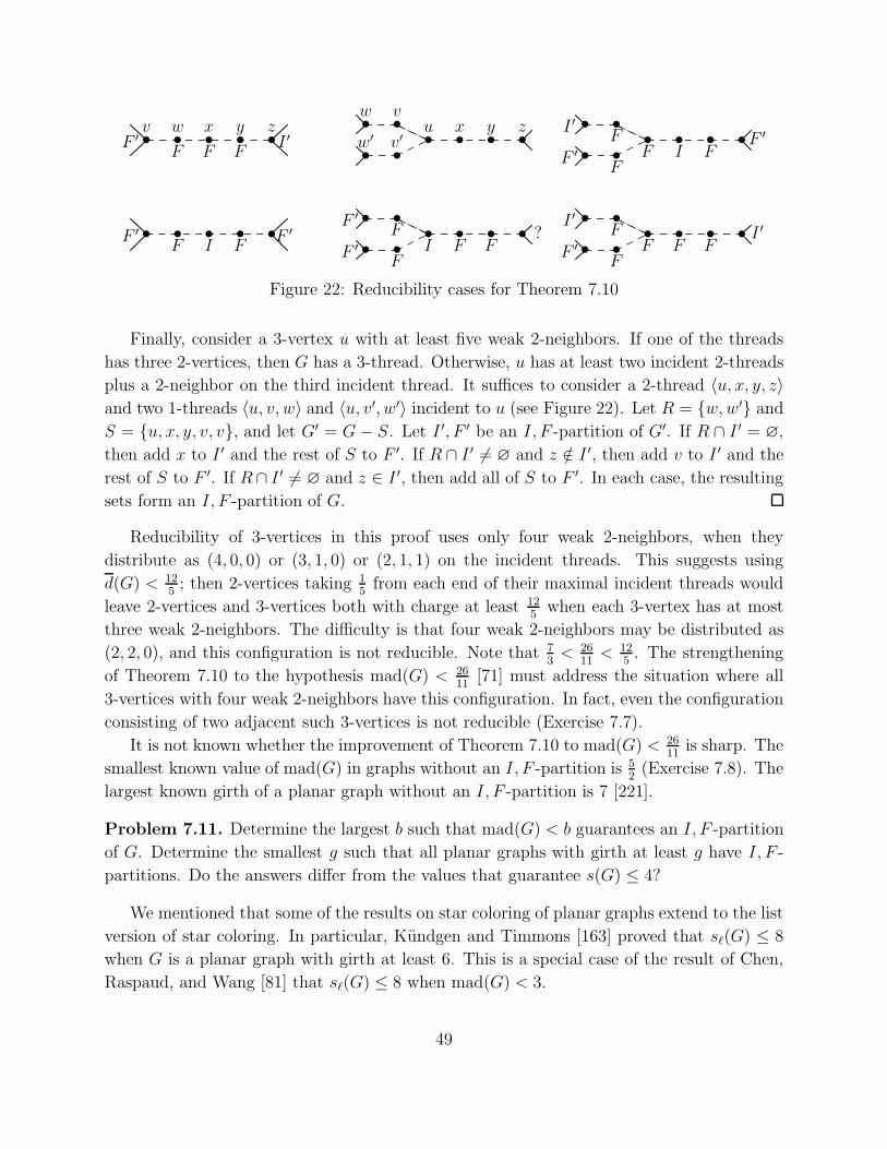
• • • • •F ′ I ′F F F
v zw x y
• • • • •F ′ F ′
F I F
• ••
••• • •w′ v′
uvw
x y z
• ••
••• • •
F ′
FI
FF ′
F F?
• ••
••• • •
F ′
FF
FI ′
I FF ′
• ••
••• • •
F ′
FF
FI ′
F FI ′
Figure 22: Reducibility cases for Theorem 7.10
Finally, consider a 3-vertex u with at least five weak 2-neighbors. If one of the threads
has three 2-vertices, then G has a 3-thread. Otherwise, u has at least two incident 2-threads
plus a 2-neighbor on the third incident thread. It suffices to consider a 2-thread 〈u, x, y, z〉and two 1-threads 〈u, v, w〉 and 〈u, v′, w′〉 incident to u (see Figure 22). Let R = w,w′ and
S = u, x, y, v, v, and let G′ = G− S. Let I ′, F ′ be an I, F -partition of G′. If R ∩ I ′ = ∅,
then add x to I ′ and the rest of S to F ′. If R ∩ I ′ 6= ∅ and z /∈ I ′, then add v to I ′ and the
rest of S to F ′. If R∩ I ′ 6= ∅ and z ∈ I ′, then add all of S to F ′. In each case, the resulting
sets form an I, F -partition of G.
Reducibility of 3-vertices in this proof uses only four weak 2-neighbors, when they
distribute as (4, 0, 0) or (3, 1, 0) or (2, 1, 1) on the incident threads. This suggests using
d(G) < 125; then 2-vertices taking 1
5from each end of their maximal incident threads would
leave 2-vertices and 3-vertices both with charge at least 125when each 3-vertex has at most
three weak 2-neighbors. The difficulty is that four weak 2-neighbors may be distributed as
(2, 2, 0), and this configuration is not reducible. Note that 73< 26
11< 12
5. The strengthening
of Theorem 7.10 to the hypothesis mad(G) < 2611
[71] must address the situation where all
3-vertices with four weak 2-neighbors have this configuration. In fact, even the configuration
consisting of two adjacent such 3-vertices is not reducible (Exercise 7.7).
It is not known whether the improvement of Theorem 7.10 to mad(G) < 2611
is sharp. The
smallest known value of mad(G) in graphs without an I, F -partition is 52(Exercise 7.8). The
largest known girth of a planar graph without an I, F -partition is 7 [221].
Problem 7.11. Determine the largest b such that mad(G) < b guarantees an I, F -partition
of G. Determine the smallest g such that all planar graphs with girth at least g have I, F -
partitions. Do the answers differ from the values that guarantee s(G) ≤ 4?
We mentioned that some of the results on star coloring of planar graphs extend to the list
version of star coloring. In particular, Kundgen and Timmons [163] proved that sℓ(G) ≤ 8
when G is a planar graph with girth at least 6. This is a special case of the result of Chen,
Raspaud, and Wang [81] that sℓ(G) ≤ 8 when mad(G) < 3.
49
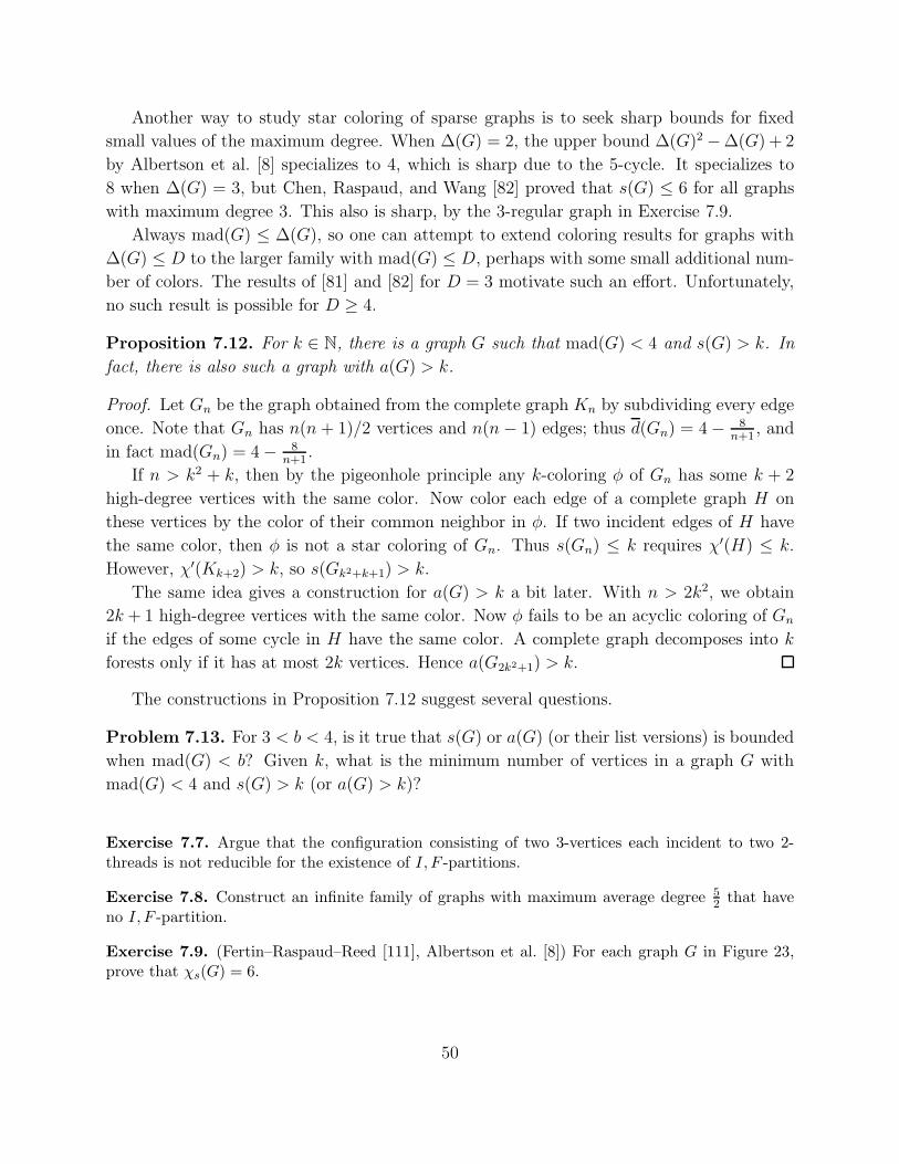
Another way to study star coloring of sparse graphs is to seek sharp bounds for fixed
small values of the maximum degree. When ∆(G) = 2, the upper bound ∆(G)2 −∆(G) + 2
by Albertson et al. [8] specializes to 4, which is sharp due to the 5-cycle. It specializes to
8 when ∆(G) = 3, but Chen, Raspaud, and Wang [82] proved that s(G) ≤ 6 for all graphs
with maximum degree 3. This also is sharp, by the 3-regular graph in Exercise 7.9.
Always mad(G) ≤ ∆(G), so one can attempt to extend coloring results for graphs with
∆(G) ≤ D to the larger family with mad(G) ≤ D, perhaps with some small additional num-
ber of colors. The results of [81] and [82] for D = 3 motivate such an effort. Unfortunately,
no such result is possible for D ≥ 4.
Proposition 7.12. For k ∈ N, there is a graph G such that mad(G) < 4 and s(G) > k. In
fact, there is also such a graph with a(G) > k.
Proof. Let Gn be the graph obtained from the complete graph Kn by subdividing every edge
once. Note that Gn has n(n + 1)/2 vertices and n(n− 1) edges; thus d(Gn) = 4− 8n+1
, and
in fact mad(Gn) = 4− 8n+1
.
If n > k2 + k, then by the pigeonhole principle any k-coloring φ of Gn has some k + 2
high-degree vertices with the same color. Now color each edge of a complete graph H on
these vertices by the color of their common neighbor in φ. If two incident edges of H have
the same color, then φ is not a star coloring of Gn. Thus s(Gn) ≤ k requires χ′(H) ≤ k.
However, χ′(Kk+2) > k, so s(Gk2+k+1) > k.
The same idea gives a construction for a(G) > k a bit later. With n > 2k2, we obtain
2k + 1 high-degree vertices with the same color. Now φ fails to be an acyclic coloring of Gn
if the edges of some cycle in H have the same color. A complete graph decomposes into k
forests only if it has at most 2k vertices. Hence a(G2k2+1) > k.
The constructions in Proposition 7.12 suggest several questions.
Problem 7.13. For 3 < b < 4, is it true that s(G) or a(G) (or their list versions) is bounded
when mad(G) < b? Given k, what is the minimum number of vertices in a graph G with
mad(G) < 4 and s(G) > k (or a(G) > k)?
Exercise 7.7. Argue that the configuration consisting of two 3-vertices each incident to two 2-threads is not reducible for the existence of I, F -partitions.
Exercise 7.8. Construct an infinite family of graphs with maximum average degree 52 that have
no I, F -partition.
Exercise 7.9. (Fertin–Raspaud–Reed [111], Albertson et al. [8]) For each graph G in Figure 23,prove that χs(G) = 6.
50
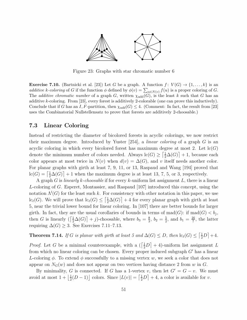
•
••••
• •• •
••
•••
•
••
Figure 23: Graphs with star chromatic number 6
Exercise 7.10. (Bartnicki et al. [23]) Let G be a graph. A function f : V (G) → 1, . . . , k is anadditive k-coloring of G if the function φ defined by φ(v) =
∑
u∈N(v) f(u) is a proper coloring of G.The additive chromatic number of a graph G, written χadd(G), is the least k such that G has anadditive k-coloring. From [23], every forest is additively 2-colorable (one can prove this inductively).Conclude that if G has an I, F -partition, then χadd(G) ≤ 4. (Comment: In fact, the result from [23]uses the Combinatorial Nullstellensatz to prove that forests are additively 2-choosable.)
7.3 Linear Coloring
Instead of restricting the diameter of bicolored forests in acyclic colorings, we now restrict
their maximum degree. Introduced by Yuster [254], a linear coloring of a graph G is an
acyclic coloring in which every bicolored forest has maximum degree at most 2. Let lc(G)
denote the minimum number of colors needed. Always lc(G) ≥⌈
12∆(G)
⌉
+ 1, because each
color appears at most twice in N(v) when d(v) = ∆(G), and v itself needs another color.
For planar graphs with girth at least 7, 9, 11, or 13, Raspaud and Wang [194] proved that
lc(G) =⌈
12∆(G)
⌉
+ 1 when the maximum degree is at least 13, 7, 5, or 3, respectively.
A graph G is linearly k-choosable if for every k-uniform list assignment L, there is a linear
L-coloring of G. Esperet, Montassier, and Raspaud [107] introduced this concept, using the
notation Λl(G) for the least such k. For consistency with other notation in this paper, we use
lcℓ(G). We will prove that lcℓ(G) ≤⌈
12∆(G)
⌉
+ 4 for every planar graph with girth at least
5, near the trivial lower bound for linear coloring. In [107] there are better bounds for larger
girth. In fact, they are the usual corollaries of bounds in terms of mad(G): if mad(G) < bj ,
then G is linearly (⌈
12∆(G)
⌉
+ j)-choosable, where b3 = 83, b2 = 5
2, and b1 = 16
7, the latter
requiring ∆(G) ≥ 3. See Exercises 7.11–7.13.
Theorem 7.14. If G is planar with girth at least 5 and ∆(G) ≤ D, then lcℓ(G) ≤⌈
12D⌉
+4.
Proof. Let G be a minimal counterexample, with a (⌈
12D⌉
+ 4)-uniform list assignment L
from which no linear coloring can be chosen. Every proper induced subgraph G′ has a linear
L-coloring φ. To extend φ successfully to a missing vertex w, we seek a color that does not
appear on NG(w) and does not appear on two vertices having distance 2 from w in G.
By minimality, G is connected. If G has a 1-vertex v, then let G′ = G − v. We must
avoid at most 1 +⌊
12(D − 1)
⌋
colors. Since |L(v)| =⌈
12D⌉
+ 4, a color is available for v.
51
We may therefore assume δ(G) ≥ 2. Since G also is planar with girth at least 5,
Lemma 7.3 implies that G has a 2-vertex v with a 5−-neighbor u or a 5-face whose inci-
dent vertices are four 3-vertices and a 5−-vertex.
In the case dG(v) = 2, let w be the other neighbor of v, and let G′ = G − v. Since
dG(u) ≤ 5, the number of forbidden colors is at most 2+⌊
(D−1)+(5−1)2
⌋
, which equals⌈
12D⌉
+3.
Since |L(v)| =⌈
12D⌉
+ 4, a color remains available for v.
Hence we may assume that G contains a 5-face whose incident vertices are 3-vertices
v1, v2, v3, v4 in cyclic order plus a 5−-vertex w. Let x2 and x3 denote the remaining neighbors
of v2 and v3, respectively, as labeled in Figure 20.
Let G′ = G − v2, v3, and let φ be a linear L-coloring of G′. Each of the two missing
vertices has two colored neighbors and at most 4 + (D − 1) colored vertices at distance 2.
Since ⌊(D + 4− 1)/2⌋ =⌈
12D⌉
+ 1, there are at most⌈
12D⌉
+ 3 colors to avoid, so for each
of v2 and v3 a color remains available.
However, each could be left with only the same single color available. To complete the
proof, we show that v2 or v3 has at least two colors available; we extend to that vertex last.
If φ(v1) = φ(x2), then v1 and x2 together forbid only one color, and v2 still has two available.
Hence we may assume φ(v1) 6= φ(x2). Similarly, we may also assume φ(v4) 6= φ(x3).
Since φ(v1) 6= φ(x2), coloring v3 cannot give v2 three neighbors with the same color. Also,
we claim that coloring v3 cannot create a 2-colored cycle. Since φ(v4) 6= φ(x3), such a cycle
must contain v2 and one of v4, x3. By requiring that v2 does not receive a color appearing
on two or more vertices at distance 2 from v2, we prevent such a 2-colored cycle.
Therefore, after extending the coloring to v2 as before, it suffices for v3 to avoid the colors
appearing on v2, x3, v4 or on at least two vertices of N(v4) ∪N(x3). The number to avoid
is at most 3 +⌊
(D−1)+22
⌋
, which equals ⌈D/2⌉ + 3. Hence a color remains available for v3.
(That is, before coloring v2, two colors were available at v3.)
A similar but more detailed argument proves lcℓ ≤⌈
12∆(G)
⌉
+ 3 when G is planar with
girth at least 5 and ∆(G) ≥ 13. To do this, we first refine Lemma 7.3 to show that if ∆(G) ≥13, then in (RC1) either a 2-vertex has a 4−-neighbor or it has a 5-neighbor and a 12−-
neighbor. Furthermore, we can require in (RC2) that at most two outside neighbors of the
four 3-vertices on the 5-face have high degree. These improvements use that faces only need13from each incident 6+-vertex v, not d(v)−4
d(v). Thus 7+-vertices have extra charge they can
send to 2-neighbors and 3-neighbors. With more careful analysis, these new configurations
are reducible even with only⌈
12∆(G)
⌉
+ 3 colors.
The problem is harder for general planar graphs, even in the non-list version. Li, Wang,
and Raspaud [169] proved that if G is planar with ∆(G) ≥ 52, then lc(G) ≤ (⌊.9∆(G)⌋+5),
dropping the coefficient below 1. Along the way, they proved lc(G) ≤ ∆(G) + 15 for all
planar G (Exercise 7.15). Finally, they asked whether there is a constant c such that lc(G) ≤⌈
12∆(G)
⌉
+ c for every planar graph G.
52
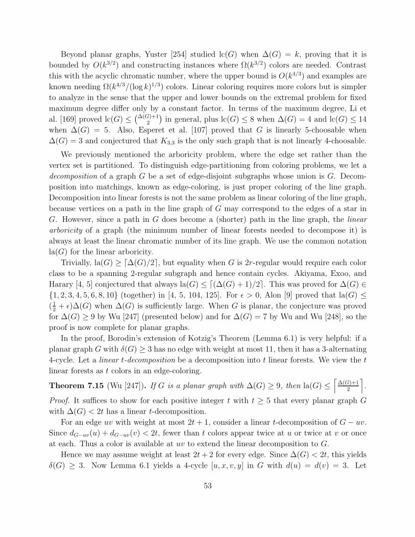
Beyond planar graphs, Yuster [254] studied lc(G) when ∆(G) = k, proving that it is
bounded by O(k3/2) and constructing instances where Ω(k3/2) colors are needed. Contrast
this with the acyclic chromatic number, where the upper bound is O(k4/3) and examples are
known needing Ω(k4/3/(log k)1/3) colors. Linear coloring requires more colors but is simpler
to analyze in the sense that the upper and lower bounds on the extremal problem for fixed
maximum degree differ only by a constant factor. In terms of the maximum degree, Li et
al. [169] proved lc(G) ≤(
∆(G)+12
)
in general, plus lc(G) ≤ 8 when ∆(G) = 4 and lc(G) ≤ 14
when ∆(G) = 5. Also, Esperet et al. [107] proved that G is linearly 5-choosable when
∆(G) = 3 and conjectured that K3,3 is the only such graph that is not linearly 4-choosable.
We previously mentioned the arboricity problem, where the edge set rather than the
vertex set is partitioned. To distinguish edge-partitioning from coloring problems, we let a
decomposition of a graph G be a set of edge-disjoint subgraphs whose union is G. Decom-
position into matchings, known as edge-coloring, is just proper coloring of the line graph.
Decomposition into linear forests is not the same problem as linear coloring of the line graph,
because vertices on a path in the line graph of G may correspond to the edges of a star in
G. However, since a path in G does become a (shorter) path in the line graph, the linear
arboricity of a graph (the minimum number of linear forests needed to decompose it) is
always at least the linear chromatic number of its line graph. We use the common notation
la(G) for the linear arboricity.
Trivially, la(G) ≥ ⌈∆(G)/2⌉, but equality when G is 2r-regular would require each color
class to be a spanning 2-regular subgraph and hence contain cycles. Akiyama, Exoo, and
Harary [4, 5] conjectured that always la(G) ≤ ⌈(∆(G) + 1)/2⌉. This was proved for ∆(G) ∈1, 2, 3, 4, 5, 6, 8, 10 (together) in [4, 5, 104, 125]. For ǫ > 0, Alon [9] proved that la(G) ≤(12+ ǫ)∆(G) when ∆(G) is sufficiently large. When G is planar, the conjecture was proved
for ∆(G) ≥ 9 by Wu [247] (presented below) and for ∆(G) = 7 by Wu and Wu [248], so the
proof is now complete for planar graphs.
In the proof, Borodin’s extension of Kotzig’s Theorem (Lemma 6.1) is very helpful: if a
planar graph G with δ(G) ≥ 3 has no edge with weight at most 11, then it has a 3-alternating
4-cycle. Let a linear t-decomposition be a decomposition into t linear forests. We view the t
linear forests as t colors in an edge-coloring.
Theorem 7.15 (Wu [247]). If G is a planar graph with ∆(G) ≥ 9, then la(G) ≤⌈
∆(G)+12
⌉
.
Proof. It suffices to show for each positive integer t with t ≥ 5 that every planar graph G
with ∆(G) < 2t has a linear t-decomposition.
For an edge uv with weight at most 2t+ 1, consider a linear t-decomposition of G− uv.
Since dG−uv(u) + dG−uv(v) < 2t, fewer than t colors appear twice at u or twice at v or once
at each. Thus a color is available at uv to extend the linear decomposition to G.
Hence we may assume weight at least 2t+2 for every edge. Since ∆(G) < 2t, this yields
δ(G) ≥ 3. Now Lemma 6.1 yields a 4-cycle [u, x, v, y] in G with d(u) = d(v) = 3. Let
53
u′ and v′ be the remaining neighbors of u and v, respectively (see Figure 24). Note that
u, v = u′, v′ is forbidden, but u′ = v′ is possible, requiring a similar analysis that we omit.
• ••
• ••
u′ u
y
v′v
x
Figure 24: Reducible configuration for Theorem 7.15
The weight restrictions and ∆(G) ≤ 2t−1 imply that each of x, y, u′, v′ has degree 2t−1
in G. Hence a linear t-decomposition of G−u, v has 2t− 3 colored edges at both x and y
and 2t− 2 colored edges at both u′ and v′. We conclude that at most one color is missing at
each of these vertices; call a vertex “bad” if a color is missing. For a vertex z, let C(z) and
C ′(z) denote the sets of colors appearing at z exactly once and at most once, respectively.
Case 1: Neither x nor y is bad. Here |C(x)| = |C(y)| = 3. First color uu′ from C ′(u′),
then ux from C(x), and then uy from C(y). Make the colors on ux and uy differ. If u′ is bad,
then the color on uu′ may be used on ux or uy, but otherwise the three edges have distinct
colors. Two colors from each of C(x) and C(y) remain, and we ensure these remaining pairs
are not equal. Now we can choose distinct colors on the three edges at v.
Case 2: One of x and y is bad. We may assume by symmetry that x is bad; still
|C(y)| = 3. Give ux the color missing at x, and give xv the one color in C(x). Color vv′
from C ′(v′), different from the color on xv if v′ is not bad. Now color vy from C(y) avoiding
the colors on xv and vv′. Now color uu′ from C ′(u′), and choose a color for uy from C(y)
avoiding that and the color on vy. Note that uu′ or uy may have the same color as ux.
Case 3: x and y are both bad. If the one missing color at each of x and y is the same,
then use it on ux and vy. Now use the color in C(x) on xv and the color in C(y) on yu. If
u′ is bad, then its missing color can be used on uu′; otherwise, color uu′ from C(u′) to avoid
the color on yu. The symmetric argument applies to color vv′.
If the missing colors at x and y are different, then use the color missing at x on ux and
xv, and use the color missing at y on uy and yv. If a color is missing at u′, use it on uu′,
and then use any color from C ′(v′) on vv′. By symmetry, then, only |C(u′)| = |C(v′)| = 2
remains, and it suffices to give uu′ and vv′ distinct colors from these sets.
Also, Wu [247] proved that la(G) =⌈
12∆(G)
⌉
when G is planar with ∆(G) ≥ 13, using a
stronger form of a lemma by Borodin (see Exercise 7.17). Cygan, Kowalik, and Luzar [98]
proved that the same conclusion holds in the larger class of planar G with ∆(G) ≥ 10, and
they conjectured that ∆(G) ≥ 6 is sufficient.
Exercise 7.11. (Esperet–Montassier–Raspaud [107]) Prove that a 1-vertex, a 3-thread, and a 3-vertex incident to three 2-threads are all reducible for lcℓ(G) ≤
⌈
12∆(G)
⌉
+ 1 when ∆(G) ≥ 3.Conclude that lcℓ(G) ≤
⌈
12∆(G)
⌉
+ 1 when mad(G) < 167 and ∆(G) ≥ 3.
54
Exercise 7.12. ([107]) Prove that a 1-vertex, a 2-thread, and a 3-vertex with three 2-neighbors areall reducible for lcℓ(G) ≤
⌈
12∆(G)
⌉
+ 2. Conclude that lcℓ(G) ≤⌈
12∆(G)
⌉
+ 2 when mad(G) < 52 .
Exercise 7.13. ([107]) Prove that a 1-vertex, a 2-thread, and a 3-vertex with two 2-neighbors areall reducible for lcℓ(G) ≤
⌈
12∆(G)
⌉
+ 3. Conclude that lcℓ(G) ≤⌈
12∆(G)
⌉
+ 3 when mad(G) < 83 .
Exercise 7.14. (van den Heuvel–McGuinness [131]) Prove that every planar graph G with δ(G) ≥ 3has a 5−-vertex v with at most two 12+-neighbors such that v has a 7−-neighbor if d(v) ∈ 4, 5,and v has an additional 6−-neighbor if d(v) = 5. (Hint: Extend the proof of Lemma 6.5 by allowing5−-vertices to take some charge from their 11−-neighbors. Comment: This is the stronger versionof Lemma 6.5 used in [131] to prove χ(G2) ≤ 2∆(G) + 25 when G is planar; see Exercise 6.13.)
Exercise 7.15. (Li–Wang–Raspaud [169]) The general bound lc(G) ≤(
∆(G)+12
)
in [169] yieldslc(G) ≤ ∆(G) + 15 when ∆(G) ≤ 6. Use Exercise 6.9 for ∆(G) ∈ 7, 8 and Exercise 7.14 for∆(G) ≥ 9 to prove lc(G) ≤ ∆(G) + 15 for every planar graph G.
Exercise 7.16. (Esperet-Montassier-Raspaud [107]) Use Exercise 7.14 to prove lcℓ(G) ≤ ∆(G)+26for every planar graph G.
Exercise 7.17. (Wu [247]) Strengthen Lemma 5.3 to show that every planar graph contains anedge of weight at most 15 or a 2-alternating cycle such that some high-degree vertex on the cyclehas an additional 2-neighbor outside the cycle. Conclude that la(G) =
⌈
12∆(G)
⌉
for every planargraph G with ∆(G) ≥ 13.
7.4 Improper Coloring
We close this section by studying a type of relaxed vertex coloring. When adjacency rep-
resents conflict, independent sets are “conflict-free”, but one may not need such a strong
restriction. There are many ways to weaken the requirements on subgraphs induced by color
classes while still remaining rather sparse; one then obtains a coloring parameter by seeking
the minimum number of such classes need to cover the vertex set.
Planar graphs are 4-colorable. Grotzsch’s Theorem gives 3-colorability for the restricted
class of triangle-free planar graphs. Alternatively, we study what relaxations of the restriction
on color classes permit successful 3-colorings.
For example, one could require that the subgraph induced by a color class have no (k+1)-
edge-connected subgraph. Setting k = 0 yields the ordinary chromatic number, and setting
k = 1 yields the parameter called vertex arboricity. As observed by Stein, a consequence of
Borodin’s acyclic 5-colorability of planar graphs is that the vertices of a planar graph can be
colored with three colors so that one class is independent and the other two induce forests.
Intermediate between independent sets and general forests are restricted forests with
bounded degree or diameter. For example, one may ask what requirement on girth in planar
graphs is needed to guarantee a 3-coloring of the vertices so that two colors induce matchings
and the third induces a forest. It would also be natural to explore what bounds on vertex
arboricity (or vertex linear arboricity) follow from mad(G) < b.
55
In the remainder of this section, we simply bound the vertex degrees in induced subgraphs.
The parameters measure how “improper” a color class is allowed to be.
Definition 7.16. A (d1, . . . , dt)-improper (or “-defective” or “-relaxed”) coloring of a graph
G is a partition of V (G) into sets V1, . . . , Vt such that ∆(G[Vi]) ≤ di for 1 ≤ i ≤ t. For
simplicity, we abbreviate the term to (d1, . . . , dt)-coloring and say that such a graph is
(d1, . . . , dt)-colorable. Without indicating the number of colors, a coloring is d-improper if
each vertex has at most d neighbors of its own color. A graph is t|d-choosable if from any
t-uniform list assignment a d-improper coloring can be chosen.
The Four Color Theorem states that every planar graph is (0, 0, 0, 0)-colorable. When
only three colors are used, we cannot guarantee (0, 0, 0)-colorings, but for i, j, k ≥ 0 we
can ask for classes of planar graphs guaranteed to be (i, j, k)-colorable or (i, j)-colorable.
The questions seem even more natural in terms of mad(G), recalling the classical result of
Lovasz [172] stating that if∑t
i∈1 di ≥ D − t+ 1, then every graph with maximum degree D
is (d1, . . . , dt)-colorable.
Cowen, Cowen, and Woodall [87] proved that every planar graph is (2, 2, 2)-colorable.
Eaton and Hull [103] and Skrekowski [211] extended this, independently proving that ev-
ery planar graph is 3|2-choosable, and Cushing and Kierstead [97] proved that they are
4|1-choosable. Skrekowski [212] proved that triangle-free planar graphs are 3|1-choosable.Toward Steinberg’s Conjecture that planar graphs without cycles of lengths 4 or 5 are 3-
colorable, it has been proved that such graphs are (1, 1, 0)-colorable [133, 250] and (3, 0, 0)-
colorable [132] (strengthening [75]); also they are 3|1-choosable [171] (see Exercise 7.23).
Graphs in the more general family forbidding only adjacent triangles and 5-cycles are (1, 1, 1)-
colorable [249]. Forbidding cycles of lengths 4 and 6 also yields (3, 0, 0)- and (1, 1, 0)-
colorings [251]. These results generally are proved by discharging.
Cowen, Goddard, and Jesurum [88] proved results on (d, . . . , d)-colorability of graphs on
higher surfaces. They also showed that recognizing (1, 1, 1)-colorability or (d, d)-colorability
is NP-complete, even for planar graphs. For lists of size 2, Skrekowski [213] proved that
planar graphs with girth at least g are 2|d-choosable for (g, d) ∈ (9, 1), (7, 2), (6, 3), (5, 4).Glebov and Zambalaeva [120] proved that planar graphs with girth at least 16 are (0, 1)-
colorable, which has been strengthened by recent work toward finding the best bounds on
mad(G) to ensure (d1, . . . , dt)-colorability. This is another way to use maximum average
degree to refine our understanding of coloring, like the problems posed in Section 2. Bounding
mad(G) is successful for (j, k)-colorability where bounding degeneracy and requiring large
girth are not: Kostochka and Nesetril [154] proved that for all j, k, g ∈ N there is a 2-
degenerate graph of girth g that is not (j, k)-colorable.
Let F (j, k) = supb : mad(G) < b implies that G is (j, k)-colorable. Note that F (0, 0) =
2, since forests are 2-colorable and odd cycles are not. The result of [154] yields F (j, k) < 4
56
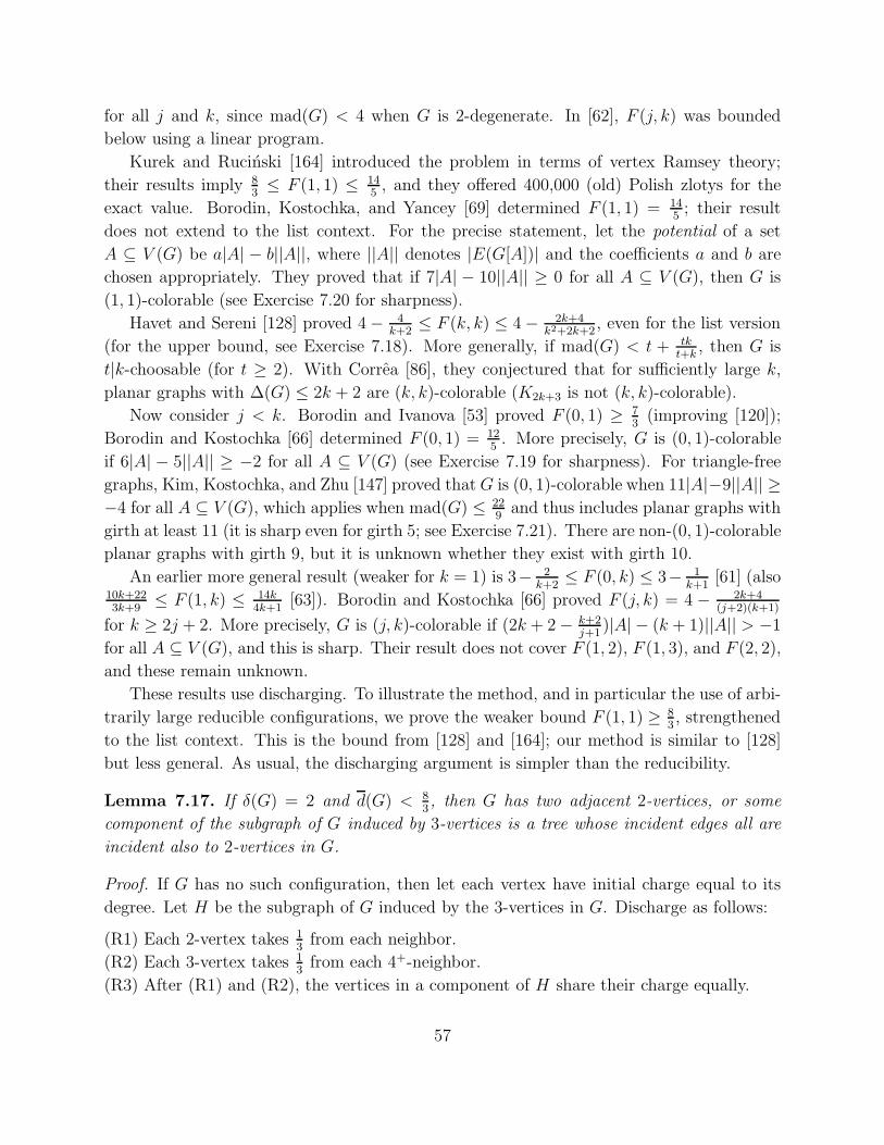
for all j and k, since mad(G) < 4 when G is 2-degenerate. In [62], F (j, k) was bounded
below using a linear program.
Kurek and Rucinski [164] introduced the problem in terms of vertex Ramsey theory;
their results imply 83≤ F (1, 1) ≤ 14
5, and they offered 400,000 (old) Polish zlotys for the
exact value. Borodin, Kostochka, and Yancey [69] determined F (1, 1) = 145; their result
does not extend to the list context. For the precise statement, let the potential of a set
A ⊆ V (G) be a|A| − b||A||, where ||A|| denotes |E(G[A])| and the coefficients a and b are
chosen appropriately. They proved that if 7|A| − 10||A|| ≥ 0 for all A ⊆ V (G), then G is
(1, 1)-colorable (see Exercise 7.20 for sharpness).
Havet and Sereni [128] proved 4− 4k+2
≤ F (k, k) ≤ 4− 2k+4k2+2k+2
, even for the list version
(for the upper bound, see Exercise 7.18). More generally, if mad(G) < t + tkt+k
, then G is
t|k-choosable (for t ≥ 2). With Correa [86], they conjectured that for sufficiently large k,
planar graphs with ∆(G) ≤ 2k + 2 are (k, k)-colorable (K2k+3 is not (k, k)-colorable).
Now consider j < k. Borodin and Ivanova [53] proved F (0, 1) ≥ 73(improving [120]);
Borodin and Kostochka [66] determined F (0, 1) = 125. More precisely, G is (0, 1)-colorable
if 6|A| − 5||A|| ≥ −2 for all A ⊆ V (G) (see Exercise 7.19 for sharpness). For triangle-free
graphs, Kim, Kostochka, and Zhu [147] proved that G is (0, 1)-colorable when 11|A|−9||A|| ≥−4 for all A ⊆ V (G), which applies when mad(G) ≤ 22
9and thus includes planar graphs with
girth at least 11 (it is sharp even for girth 5; see Exercise 7.21). There are non-(0, 1)-colorable
planar graphs with girth 9, but it is unknown whether they exist with girth 10.
An earlier more general result (weaker for k = 1) is 3− 2k+2
≤ F (0, k) ≤ 3− 1k+1
[61] (also10k+223k+9
≤ F (1, k) ≤ 14k4k+1
[63]). Borodin and Kostochka [66] proved F (j, k) = 4 − 2k+4(j+2)(k+1)
for k ≥ 2j + 2. More precisely, G is (j, k)-colorable if (2k + 2− k+2j+1
)|A| − (k + 1)||A|| > −1
for all A ⊆ V (G), and this is sharp. Their result does not cover F (1, 2), F (1, 3), and F (2, 2),
and these remain unknown.
These results use discharging. To illustrate the method, and in particular the use of arbi-
trarily large reducible configurations, we prove the weaker bound F (1, 1) ≥ 83, strengthened
to the list context. This is the bound from [128] and [164]; our method is similar to [128]
but less general. As usual, the discharging argument is simpler than the reducibility.
Lemma 7.17. If δ(G) = 2 and d(G) < 83, then G has two adjacent 2-vertices, or some
component of the subgraph of G induced by 3-vertices is a tree whose incident edges all are
incident also to 2-vertices in G.
Proof. If G has no such configuration, then let each vertex have initial charge equal to its
degree. Let H be the subgraph of G induced by the 3-vertices in G. Discharge as follows:
(R1) Each 2-vertex takes 13from each neighbor.
(R2) Each 3-vertex takes 13from each 4+-neighbor.
(R3) After (R1) and (R2), the vertices in a component of H share their charge equally.
57
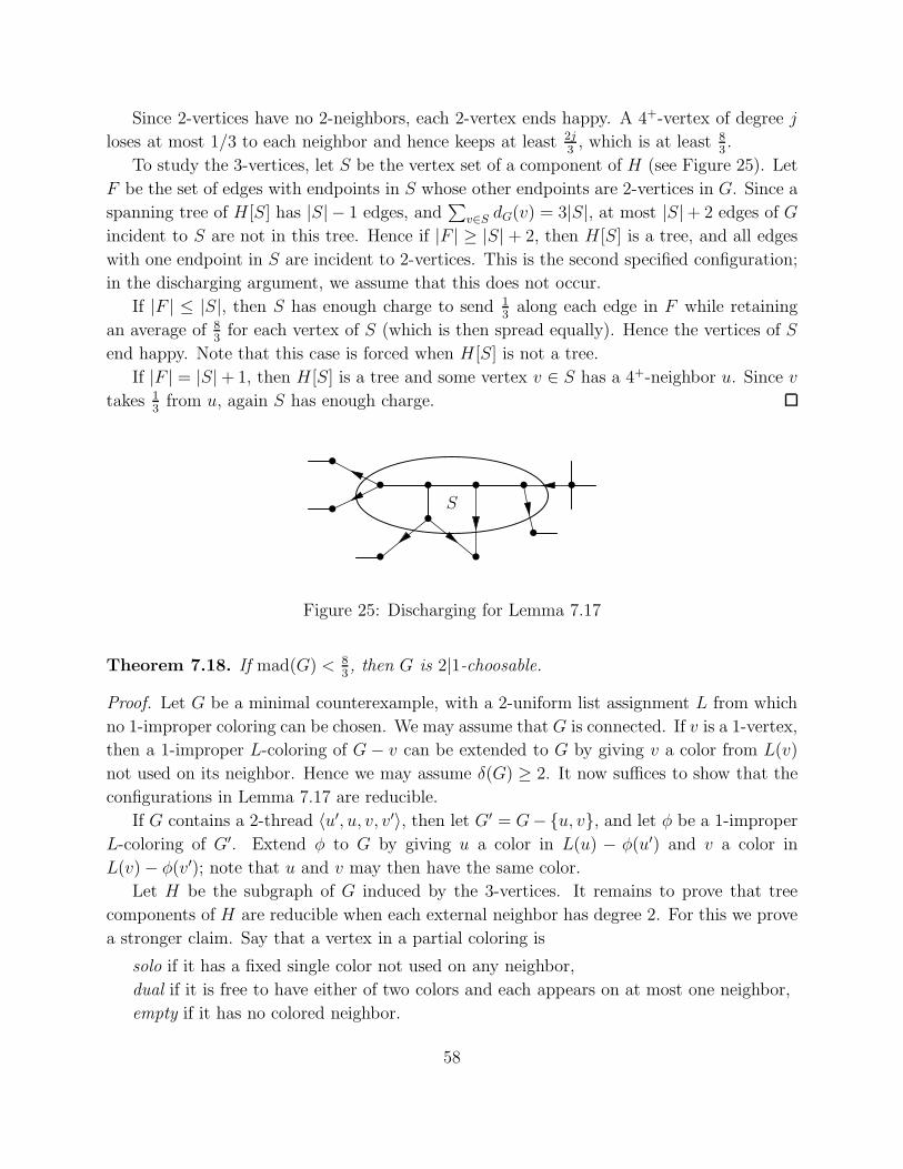
Since 2-vertices have no 2-neighbors, each 2-vertex ends happy. A 4+-vertex of degree j
loses at most 1/3 to each neighbor and hence keeps at least 2j3, which is at least 8
3.
To study the 3-vertices, let S be the vertex set of a component of H (see Figure 25). Let
F be the set of edges with endpoints in S whose other endpoints are 2-vertices in G. Since a
spanning tree of H [S] has |S| − 1 edges, and∑
v∈S dG(v) = 3|S|, at most |S|+ 2 edges of G
incident to S are not in this tree. Hence if |F | ≥ |S|+ 2, then H [S] is a tree, and all edges
with one endpoint in S are incident to 2-vertices. This is the second specified configuration;
in the discharging argument, we assume that this does not occur.
If |F | ≤ |S|, then S has enough charge to send 13along each edge in F while retaining
an average of 83for each vertex of S (which is then spread equally). Hence the vertices of S
end happy. Note that this case is forced when H [S] is not a tree.
If |F | = |S|+ 1, then H [S] is a tree and some vertex v ∈ S has a 4+-neighbor u. Since v
takes 13from u, again S has enough charge.
•
•• •
•
• •
• •
•
•S
Figure 25: Discharging for Lemma 7.17
Theorem 7.18. If mad(G) < 83, then G is 2|1-choosable.
Proof. Let G be a minimal counterexample, with a 2-uniform list assignment L from which
no 1-improper coloring can be chosen. We may assume that G is connected. If v is a 1-vertex,
then a 1-improper L-coloring of G− v can be extended to G by giving v a color from L(v)
not used on its neighbor. Hence we may assume δ(G) ≥ 2. It now suffices to show that the
configurations in Lemma 7.17 are reducible.
If G contains a 2-thread 〈u′, u, v, v′〉, then let G′ = G−u, v, and let φ be a 1-improper
L-coloring of G′. Extend φ to G by giving u a color in L(u) − φ(u′) and v a color in
L(v)− φ(v′); note that u and v may then have the same color.
Let H be the subgraph of G induced by the 3-vertices. It remains to prove that tree
components of H are reducible when each external neighbor has degree 2. For this we prove
a stronger claim. Say that a vertex in a partial coloring is
solo if it has a fixed single color not used on any neighbor,
dual if it is free to have either of two colors and each appears on at most one neighbor,
empty if it has no colored neighbor.
58
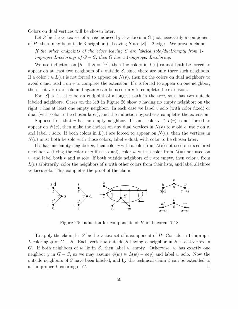
Colors on dual vertices will be chosen later.
Let S be the vertex set of a tree induced by 3-vertices in G (not necessarily a component
of H ; there may be outside 3-neighbors). Leaving S are |S|+ 2 edges. We prove a claim:
If the other endpoints of the edges leaving S are labeled solo/dual/empty from 1-
improper L-colorings of G− S, then G has a 1-improper L-coloring.
We use induction on |S|. If S = v, then the colors in L(v) cannot both be forced to
appear on at least two neighbors of v outside S, since there are only three such neighbors.
If a color c ∈ L(v) is not forced to appear on N(v), then fix the colors on dual neighbors to
avoid c and used c on v to complete the extension. If c is forced to appear on one neighbor,
then that vertex is solo and again c can be used on v to complete the extension.
For |S| > 1, let v be an endpoint of a longest path in the tree, so v has two outside
labeled neighbors. Cases on the left in Figure 26 show v having no empty neighbor; on the
right v has at least one empty neighbor. In each case we label v solo (with color fixed) or
dual (with color to be chosen later), and the induction hypothesis completes the extension.
Suppose first that v has no empty neighbor. If some color c ∈ L(v) is not forced to
appear on N(v), then make the choices on any dual vertices in N(v) to avoid c, use c on v,
and label v solo. If both colors in L(v) are forced to appear on N(v), then the vertices in
N(v) must both be solo with those colors; label v dual, with color to be chosen later.
If v has one empty neighbor w, then color v with a color from L(v) not used on its colored
neighbor u (fixing the color of u if u is dual), color w with a color from L(w) not used on
v, and label both v and w solo. If both outside neighbors of v are empty, then color v from
L(v) arbitrarily, color the neighbors of v with other colors from their lists, and label all three
vertices solo. This completes the proof of the claim.
••
• ••
• •
•v↑→
u w
z′
z
•
•
•S
•
••
s|d
v s
d
z′
z
•
••
s
v d
s
z′
z•
••u
vw
s|ds
e→s
••
•w′v
w
e→ss
e→s
Figure 26: Induction for components of H in Theorem 7.18
To apply the claim, let S be the vertex set of a component of H . Consider a 1-improper
L-coloring φ of G − S. Each vertex w outside S having a neighbor in S is a 2-vertex in
G. If both neighbors of w lie in S, then label w empty. Otherwise, w has exactly one
neighbor y in G − S, so we may assume φ(w) ∈ L(w) − φ(y) and label w solo. Now the
outside neighbors of S have been labeled, and by the technical claim φ can be extended to
a 1-improper L-coloring of G.
59
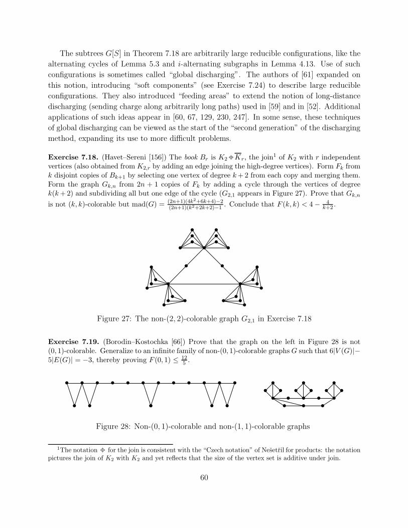
The subtrees G[S] in Theorem 7.18 are arbitrarily large reducible configurations, like the
alternating cycles of Lemma 5.3 and i-alternating subgraphs in Lemma 4.13. Use of such
configurations is sometimes called “global discharging”. The authors of [61] expanded on
this notion, introducing “soft components” (see Exercise 7.24) to describe large reducible
configurations. They also introduced “feeding areas” to extend the notion of long-distance
discharging (sending charge along arbitrarily long paths) used in [59] and in [52]. Additional
applications of such ideas appear in [60, 67, 129, 230, 247]. In some sense, these techniques
of global discharging can be viewed as the start of the “second generation” of the discharging
method, expanding its use to more difficult problems.
Exercise 7.18. (Havet–Sereni [156]) The book Br is K2 Kr, the join1 of K2 with r independentvertices (also obtained from K2,r by adding an edge joining the high-degree vertices). Form Fk fromk disjoint copies of Bk+1 by selecting one vertex of degree k + 2 from each copy and merging them.Form the graph Gk,n from 2n + 1 copies of Fk by adding a cycle through the vertices of degreek(k + 2) and subdividing all but one edge of the cycle (G2,1 appears in Figure 27). Prove that Gk,n
is not (k, k)-colorable but mad(G) = (2n+1)(4k2+6k+4)−2(2n+1)(k2+2k+2)−1
. Conclude that F (k, k) < 4 − 4k+2 .
• •••••
•••
•
•
•
••••••
•
•
•
•••
•••
• •
Figure 27: The non-(2, 2)-colorable graph G2,1 in Exercise 7.18
Exercise 7.19. (Borodin–Kostochka [66]) Prove that the graph on the left in Figure 28 is not(0, 1)-colorable. Generalize to an infinite family of non-(0, 1)-colorable graphs G such that 6|V (G)|−5|E(G)| = −3, thereby proving F (0, 1) ≤ 12
5 .
• • • • • •
• • •
••••••
•••
•••
• • ••••• ••••
•••
Figure 28: Non-(0, 1)-colorable and non-(1, 1)-colorable graphs
1The notation for the join is consistent with the “Czech notation” of Nesetril for products: the notationpictures the join of K2 with K2 and yet reflects that the size of the vertex set is additive under join.
60
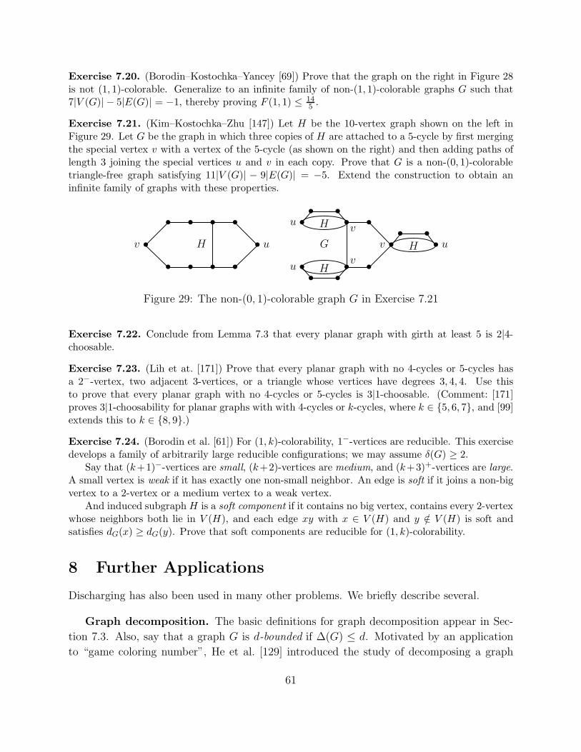
Exercise 7.20. (Borodin–Kostochka–Yancey [69]) Prove that the graph on the right in Figure 28is not (1, 1)-colorable. Generalize to an infinite family of non-(1, 1)-colorable graphs G such that7|V (G)| − 5|E(G)| = −1, thereby proving F (1, 1) ≤ 14
5 .
Exercise 7.21. (Kim–Kostochka–Zhu [147]) Let H be the 10-vertex graph shown on the left inFigure 29. Let G be the graph in which three copies of H are attached to a 5-cycle by first mergingthe special vertex v with a vertex of the 5-cycle (as shown on the right) and then adding paths oflength 3 joining the special vertices u and v in each copy. Prove that G is a non-(0, 1)-colorabletriangle-free graph satisfying 11|V (G)| − 9|E(G)| = −5. Extend the construction to obtain aninfinite family of graphs with these properties.
•
• • •
•
•••
•
•
v uH
• •
• •
• •
•
•
H
H
H
u
u
u
v
v
vG
• •
• •
• •
Figure 29: The non-(0, 1)-colorable graph G in Exercise 7.21
Exercise 7.22. Conclude from Lemma 7.3 that every planar graph with girth at least 5 is 2|4-choosable.
Exercise 7.23. (Lih et at. [171]) Prove that every planar graph with no 4-cycles or 5-cycles hasa 2−-vertex, two adjacent 3-vertices, or a triangle whose vertices have degrees 3, 4, 4. Use thisto prove that every planar graph with no 4-cycles or 5-cycles is 3|1-choosable. (Comment: [171]proves 3|1-choosability for planar graphs with with 4-cycles or k-cycles, where k ∈ 5, 6, 7, and [99]extends this to k ∈ 8, 9.)
Exercise 7.24. (Borodin et al. [61]) For (1, k)-colorability, 1−-vertices are reducible. This exercisedevelops a family of arbitrarily large reducible configurations; we may assume δ(G) ≥ 2.
Say that (k+1)−-vertices are small, (k+2)-vertices are medium, and (k+3)+-vertices are large.A small vertex is weak if it has exactly one non-small neighbor. An edge is soft if it joins a non-bigvertex to a 2-vertex or a medium vertex to a weak vertex.
And induced subgraph H is a soft component if it contains no big vertex, contains every 2-vertexwhose neighbors both lie in V (H), and each edge xy with x ∈ V (H) and y /∈ V (H) is soft andsatisfies dG(x) ≥ dG(y). Prove that soft components are reducible for (1, k)-colorability.
8 Further Applications
Discharging has also been used in many other problems. We briefly describe several.
Graph decomposition. The basic definitions for graph decomposition appear in Sec-
tion 7.3. Also, say that a graph G is d-bounded if ∆(G) ≤ d. Motivated by an application
to “game coloring number”, He et al. [129] introduced the study of decomposing a graph
61
into a forest and a d-bounded subgraph. Many papers proved such results for planar graphs
under girth restrictions and then for bounded mad(G). Montassier et al. [182] observed that
subdividing each edge of a (2d+2)-regular graph yields a graph with average degree 2+ 2dd+2
having no decomposition into a forest and a d-bounded graph. They asked for the largest
b such that mad(G) < b is sufficient, showing that 2d+4d+6+6/d
is sufficient. These results were
proved by discharging, with [182] using pots of charge corresponding to special subgraphs.
Kim et al. [148] proved that the construction in [182] is sharp: mad(G) < 2 + 2dd+2
guarantees decomposition into a forest and a d-bounded graph. Although this implies the
earlier results for planar graphs with large girth, it was not proved by discharging. Instead, a
more detailed statement allowing differing bounds on vertex degrees in the d-bounded graph
was proved inductively, using potential functions such as those defined in Section 7.4.
Montassier et al. [181] asked what restriction on mad(G) guarantees a decomposition
into k + 1 forests, with one required to be d-bounded? Recall from Theorem 6.6 that G
decomposes into k forests if and only if ⌈Arb(G)⌉ ≤ k, where Arb(G) = maxH⊆G|E(H)|
|V (H)|−1.
Intuitively, if the fractional arboricity Arb(G) just slightly exceeds k, then it should be
possible to control the last forest. The Nine Dragon Tree2 Conjecture [181] asserts that if
Arb(G) ≤ k + dk+d+1
, then G decomposes into k + 1 forests with one being d-bounded.
The conjecture was proved when k = 1 for d ≤ 2 in [181] and for d ≤ 6 in [148].
These proofs used discharging and potential functions. When d > k, [148] proved that
Arb(G) ≤ k+ dk+d+1
suffices for decomposability of G into k forests plus one d-bounded graph
(not necessarily a forest). This hypothesis is a bit stronger than mad(G) < 2k+ 2dk+d+1
. The
result was first proved by discharging, but the inductive proof of a more detailed statement
about potential functions is much shorter.
For d ≤ k + 1, the stronger restriction Arb(G) ≤ k + d2k+2
implies the conclusion of the
NDT Conjecture ([148]). Since d2k+2
= dk+d+1
when d = k + 1, the NDT Conjecture is thus
true in that case. The technique here again was inductive.
The Strong NDT Conjecture asserts that under the same arboricity restriction, the last
forest can also be required to have at most d edges in each component. Equivalent to the
NDT Conjecture when d = 1, this has been proved for (k, d) = (1, 2) [148].
When k = 3, Balogh et al. [22] proved that every planar graph decomposes into three
forests with one being 8-bounded (recall Exercise 6.11). They conjectured that 8 can be
improved to 4, which Goncalves [121] proved; this does not follow from [148]. Goncalves [121]
also proved that planar graphs with girth at least g decompose into two forests with one
being d-bounded, for (g, d) = (6, 4) or (g, d) = (7, 2); these results do follow from [148].
Other graph properties. The subject of homomorphism, introduced in Section 2,
includes the subject of coloring, but in full generality it is not as thoroughly developed.
Nevertheless, there are analogous results. Dvorak, Skrekovski, and Valla [102] proved that
2The Nine Dragon Tree, a banyan tree atop a mountain in Kaohsiung, Taiwan, is far from acyclic.
62
every planar graph G having no odd cycle of length less than 9 is H-colorable, where H is
the Petersen graph (that is, there is a homomorphism from G to the Petersen graph). The
proof involves a quite length discharging argument. Note that being H-colorable is stronger
than being 3-colorable when H is 3-colorable.
It remains unknown whether 9 can be improved to 7. It cannot be improved to 5;
the graph obtained from K4 by doubly subdividing the two edges of a matching is not
H-colorable. This graph has average degree 52; Chen and Raspaud [77] proved (again by
a substantial discharging argument) that every triangle-free graph with mad(G) < 52is H-
colorable. As a weaker version of the conjecture that planar graphs with girth at least 4t have
circular chromatic number at most 2 + 1t, they conjectured that such graphs have fractional
chromatic number at most 2 + 1t, and the result of [102] confirms this for t = 2.
A set S ⊆ V (G) is dominating in a graph G if every vertex in V (G) \ S has a neigh-
bor in S. The domination number γ(G) is the size of the smallest dominating set in G.
Reed [192] proved γ(G) ≤ 38n for every n-vertex graph G with δ(G) ≥ 3. The proof assumes
a counterexample G and covers G with vertex disjoint paths, subject to various minimality
conditions. The desired dominating set now consists of roughly every third vertex on each
path (with special attention to the endpoints).
Careful counting of the edges from the endpoints is needed. Discharging can provide
a convenient language in which to present counting arguments that involve inequalities.
Kostochka and Stodolsky [157] used this approach to strengthen Reed’s argument, proving
that 3-regular graphs have dominating sets using at most 411
of their vertices. Beginning with
charge 1 at each vertex of a dominating set and charge 0 elsewhere, they redistributed charge
so that each vertex finished with charge at most 411. By further developing this discharging
approach, Kostochka and Stocker [155] reduced the ratio to 514.
Discharging has also been used to prove non-local structural properties of graphs that
are sparse by virture of being embedded in surfaces. For example, Sanders and Zhao [201]
proved that every graph that embeds in a surface of Euler characteristic k has a spanning
2-connected subgraph with maximum degree at most 10 − 2k. For k ≤ 10, they improved
this to the best possible 6− 2k. The proof is by discharging.
For a graph G, the edge-deck is the multiset G − e : e ∈ E(G). A graph G is edge-
reconstructible if G is uniquely determined by its edge-deck. In 1964, Harary conjectured that
every graph with at least four edges is edge-reconstructible. Zhao [256, 257] applied discharg-
ing to the special case of Harary’s Edge-Reconstruction Conjecture for graphs embedded on
sufaces. Building on work of Fiorini and Lauri, he proved that if G is a triangulation of a
surface with Euler characteristic k and |V (G)| ≥ −43k, then G is edge-reconstructible.
A “planar cover” of a graph G is a homomorphism from a planar graph to G that maps
vertex neighborhoods bijectively. A number of papers have applied discharging to Negami’s
Conjecture that a graph has a finite planar cover if and only if it embeds in the projective
63
plane; they are surveyed by Hlineny [134], who wrote many of them.
We also mention some classical graph-theoretic problems not involving coloring or em-
beddings on surfaces. A well-known conjecture by Thomassen [218] asserts that every 4-
connected line graph is Hamiltonian. In this direction, Li and Yang [170] proved that every
3-connected, essentially 10-connected line graph is Hamiltonian-connected. Lai, Wang, and
Zhan [167] then gave a proof of this result by discharging.
Belotserkovsky [31] used discharging to determine the minimum number of edges in a
2-connected graph with n vertices and diameter at most d, when n is sufficently large: it is⌈
dn−2d−1d−1
⌉
.
Let ν(G) denote the maximum number of pairwise edge-disjoint triangles in a graph G,
and let τ(G) denote the minimum number of edges needed to hit all the triangles. Trivially,
ν(G) ≤ τ(G) ≤ 3ν(G). Tuza [222] conjectured that always τ(G) ≤ 2ν(G), which is sharp
for a graph consisting of edge-disjoint copies of K4. Tuza [223] proved the conjecture for
planar graphs, and Krivelevich [160] proved it for all 4-colorable graphs. Extending Tuza’s
result in a different direction, Puleo [193] used discharging to prove the conjecture whenever
mad(G) < 7.
Topological graphs. Radoicic and Toth [191] described various uses of discharging
in combinatorial geometry, starting with a short, clever (non-inductive!) proof of Euler’s
Formula itself found by Thurston [220]. They gave an extensive summary of coloring topics
on plane graphs before moving on to discrete geometry, where they proved a special case of
a conjecture of Pach and Sharir [189]: If H is a bipartite graph, then there is a constant
cH such that every H-avoiding intersection graph of n convex sets in the plane has at most
cHn edges, where a graph is H-avoiding if it does not contain H . Radoicic and Toth used
discharging to prove the conjecture for H ∈ K2,3, C6.To motivate their proof, Radoicic and Toth described the discharging proof by Ackerman
and Tardos [2] about the maximum number of edges in quasi-planar graphs. A topological
graph is a graph drawn in the plane; it is a geometric graph when the edges are drawn as
line segments. A topological graph is k-quasi-planar if it does not have k pairwise crossing
edges. Thus a 2-quasi-planar graph is a plane graph, and 3-quasi-planar graphs are simply
called quasi-planar.
Capolyeas and Pach [74] conjectured for every fixed k that the maximum number of
edges in a k-quasi-planar graph on n vertices is linear in n. Agarwal et al. [3] proved this for
k = 3, and Ackerman [1] proved it for k = 4 (by discharging). The short discharging proof
by Ackerman and Tardos [2] gave a much better bound on the coefficient for k = 3: there
are at most 8n− 20 edges. A construction gave a lower bound of 7n− O(√n) edges. They
used two rounds of discharging and noted that stopping after the first round still yields an
upper bound of 10n− 20.
The discharging ideas are unusual. First draw the graph G with the fewest crossings.
64
The fact that G is 3-quasi-planar implies that in the graph G′ obtained by introducing new
vertices for the crossings, the new vertices are all 4-vertices and every 3-face contains at least
one original vertex. Assign charge l(f)− 4 + v(f) to each face f of G′, where v(f) denotes
the number of original vertices incident to f . The desire is for each face f to have charge
at least v(f)5, after which the second round proceeds. The only faces that do not have this
much charge are triangles having only one original vertex u. Such a face f defines a channel
between its boundary edges e and e′ that are incident to u. Basically, f takes 15from the
first face along this channel that is not a 4-face having no original vertices.
Ackerman and Tardos [2] also provided a very short discharging proof that bounds the
number of edges of the multigraph G by 19n, using balanced charging on G′. In a minimal
counterexample, each vertex of G has degree at least 20. Every original vertex sends 45to
each incident face. Every 3-face in G′ that has only one original vertex takes 15in the same
way as above. Since δ(G) ≥ 20, each vertex remains happy.
Sharir and Welzl [207] used discharging to prove that the number of triangulations (with
straight edges) of a set of n points in the plane is at most 43n. Sharir and Sheffer [206]
refined this approach to improve the upper bound to 30n. For a set S of n points in the
plane, their methods also bound the number of planar straight-line graphs on S in various
classes, including all planar graphs (207.84n), spanning cycles (O(68.67n)), spanning trees
(O(146.69n)), and forests (O(164.17n)).
Given a planar n-point set S, their basic idea is to prove a lower bound on the average
number of 3-vertices in a uniformly chosen triangulation of S. Their approach is complicated,
so we just present a brief sketch; for more detail, see Sections 2 and 3 of [206]. They show
that if the average number of 3-vertices in such a triangulation is at least cn for some positive
constant c, then the total number of triangulations of S is at most c−n. To prove a lower
bound on the average number of 3-vertices, each 4+-vertex sends total charge at least 1 to 3-
vertices, and each 3-vertex receives charge at most 1/c. Much of the work consists of proving
an upper bound on the charge received by each 3-vertex. The innovation that allows this
approach to work is sending charge between triangulations. Since some triangulations have
no 3-vertices, each 4+-vertex in such a triangulation sends charge to 3-vertices in “nearby”
triangulations (under an appropriate edge-flipping metric).
References
[1] E. Ackerman, On the maximum number of edges in topological graphs with no four pairwise crossingedges, Discrete Comput. Geom. 41 (2009), no. 3, 365–375.
[2] E. Ackerman and G. Tardos, On the maximum number of edges in quasi-planar graphs, J. Combin.Theory Ser. A 114 (2007), no. 3, 563–571.
[3] P.K. Agarwal, B. Aronov, J. Pach, R. Pollack, and M Sharir, Quasi-planar graphs have a linear numberof edges, Combinatorica 17 (1997), no. 1, 1–9.
65
[4] J. Akiyama, G. Exoo, and F. Harary, Covering and packing in graphs III: Cyclic and acyclic invariants,Math Slovaca 30 (1980), 405–417.
[5] J. Akiyama, G. Exoo, and F. Harary, Covering and packing in graphs. IV. Linear arboricity, Networks11 (1981), no. 1, 69–72.
[6] M.O. Albertson, A lower bound for the independence number of a planar graph, J. Combin. TheorySer. B 20 (1976), no. 1, 84–93.
[7] M.O. Albertson and D.M. Berman, Every planar graph has an acyclic 7-coloring, Israel J. Math. 28(1977), no. 1–2, 169–174.
[8] M.O. Albertson, G.G. Chappell, H.A. Kierstead, A. Kundgen, and R. Ramamurthi, Coloring with no2-colored P4’s, Electron. J. Combin. 11 (2004), no. 1, Research Paper 26, 13 pp.
[9] N. Alon, The linear arboricity of graphs, Israel J. Math. 62 (1988), 311–325.
[10] N. Alon, C. McDiarmid, and B. Reed, Acyclic coloring of graphs, Random Structures & Algorithms 2
(1991), no. 3, 277–288.
[11] N. Alon, B. Sudakov, and A. Zaks, Acyclic edge colorings of graphs, J. Graph Theory 37 (2001), no.3, 157–167.
[12] L. D. Andersen, E. Macajova, J. Mazak, Optimal acyclic edge-coloring of cubic graphs, J. Graph Theory71 (2012), no. 4, 353–364.
[13] K. Appel and W. Haken, Every planar map is four colorable. I. Discharging, Illinois J. Math. 21 (1977),no. 3, 429–490.
[14] K. Appel and W. Haken, Supplement to: “Every planar map is four colorable. I. Discharging” (IllinoisJ. Math. 21 (1977), no. 3, 429490) by Appel and Haken; “II. Reducibility” (ibid. 21 (1977), no. 3,491567) by Appel, Haken and Koch, Illinois J. Math. 21 (1977), no. 3, 1251. (microfiche supplement).
[15] K. Appel and W. Haken, The class check lists corresponding to the supplement: “Every planar map isfour colorable. I. Discharging” (Illinois J. Math. 21 (1977), no. 3, 429490), Illinois J. Math. 21 (1977),no. 3, C1-C210. (microfiche supplement).
[16] K. Appel and W. Haken, K. Appel and W. Haken, The class check lists corresponding to the supplement:“Every planar map is four colorable. I. Discharging” (Illinois J. Math. 21 (1977), no. 3, 429490), IllinoisJ. Math. 21 (1977), no. 3, C1-C210. (microfiche supplement).
[17] K. Appel and W. Haken, An unavoidable set of configurations in planar triangulations, J. Combin.Theory Ser. B 26 (1979), no. 1, 1–21.
[18] K. Appel and W. Haken, The four color proof suffices, Math. Intelligencer 8 (1986), no. 1, 10–20, 58.
[19] K. Appel and W. Haken, Every planar map is four colorable, with the collaboration of J. Koch,Contemporary Mathematics 98, American Mathematical Society, Providence, RI, 1989. xvi+741 pp.
[20] K. Appel, W. Haken, and J. Koch, Every planar map is four colorable. II. Reducibility, Illinois J.Math. 21 (1977), no. 3, 491–567.
[21] K. Appel, W. Haken, and J. Mayer, Triangulation a v5 separes dans le probleme des quatre couleurs,J. Combin. Theory Ser. B 27 (1979), no. 2, 130–150 [French].
[22] J. Balogh, M. Kochol, A. Pluhar, and X. Yu, Covering planar graphs with forests, J. Combin. TheorySer. B 94 (2005), no. 1, 147–158.
[23] T. Bartnicki, B. Bosek, S. Czerwinski, J. Grytczuk, G. Matecki, and W. Zelazny, Additive colorings ofplanar graphs, preprint, available at: http://arxiv.org/abs/1202.0667.
[24] M. Basavaraju and L.S. Chandran, Acyclic edge coloring of subcubic graphs, Discrete Math. 308 (2008),no. 24, 6650–6653.
66
[25] M. Basavaraju and L.S. Chandran, Acyclic edge coloring of graphs with maximum degree 4, J. GraphTheory 61 (2009), no. 3, 192–209.
[26] M. Basavaraju and L.S. Chandran, A note on acyclic edge coloring of complete bipartite graphs,Discrete Math. 309 (2009), no. 13, 4646–4648.
[27] M. Basavaraju and L.S. Chandran, Acyclic edge coloring of triangle-free planar graphs, J. Graph Theory71 (2012), no. 4, 365–385.
[28] M. Basavaraju, L.S. Chandran, N. Cohen, F. Havet, and T. Muller, Acyclic edge-coloring of planargraphs, SIAM J. Discrete Math. 25 (2011), no. 2, 463–478.
[29] M. Basavaraju, L.S. Chandran, and M. Kummini, d-regular graphs of acyclic chromatic index at leastd+2, J. Graph Theory 63 (2010), no. 3, 226–230.
[30] M. Behzad, Graphs and Their Chromatic Numbers, Ph.D. thesis, Michigan State Univ., 1965.
[31] D. Belotserkovsky, The smallest number of edges in a 2-connected graph with specified diameter,Discrete Math. 307 (2007), no. 19-20, 2376–2384.
[32] B. Bollobas and A.J. Harris, List-colourings of graphs, Graphs Combin. 1 (1985), 115–127.
[33] M. Bonamy, Planar graphs with maximum degree D at least 8 are (D + 1)-edge-choosable, preprint,available at: http://arxiv.org/abs/1303.4025.
[34] M. Bonamy, B. Leveque, and A. Pinlou, Graphs with maximum degree D at least 17 andmaximum average degree less than 3 are list 2-distance (D+2)-colorable, preprint, available at:http://arxiv.org/abs/1301.7090.
[35] M. Bonamy, B. Leveque, and A. Pinlou, 2-distance coloring of sparse graphs, preprint, available at:http://www.lirmm.fr/~pinlou/wordpress/wp-content/papercite-data/pdf/blp12.pdf.
[36] O.V. Borodin, On acyclic colorings of planar graphs, Discrete Math. 25 (1979), no. 3, 211–236.
[37] O.V. Borodin, Solution of the Ringel problem on vertex-face coloring of planar graphs and coloring of1-planar graphs, Metody Diskret. Analiz. 41 (1984), 12–26, 108 [Russian].
[38] O.V. Borodin, Coupled colorings of graphs on a plane, Metody Diskret. Analiz. 45 (1987), 21–27 [Rus-sian].
[39] O.V. Borodin, On the total coloring of planar graphs, J. Reine Angew. Math. 394 (1989), 180–185.
[40] O.V. Borodin, Solving the Kotzig and Grunbaum problems on the separability of a cycle in planargraphs, Mat. Zametki 46 (1989), no. 5, 9–12, 103 [Russian]; translation in Math. Notes 46 (1989), no.5-6, 835–837 (1990).
[41] O.V. Borodin, A generalization of Kotzig’s theorem and prescribed edge coloring of planar graphs,Mat. Zametki 48 (1990), no. 6, 22–28, 160 [Russian]; translation in Math. Notes 48 (1990), no. 5-6,1186–1190 (1991).
[42] O.V. Borodin, A new proof of the 6 color theorem, J. Graph Theory 19 (1995), no. 4, 507–521.
[43] O.V. Borodin, Structural properties of plane graphs without adjacent triangles and an application to3-colorings, J. Graph Theory 21 (1996), no. 2, 183–186.
[44] O.V. Borodin, Structural theorem on plane graphs with application to the entire coloring number, J.Graph Theory 23 (1996), no. 3, 233–239.
[45] O.V. Borodin, Colorings of plane graphs: A survey, Discrete Math. 313 (2013), no. 4, 517–539.
[46] O. V. Borodin, H. J. Broersma, A. Glebov, and J. van den Heuvel, Stars and bunches inplanar graphs, Part I: Triangulations, CDAM Research Report Series 2002–04 (2002). Origi-nal Russian version. Diskretn. Anal. Issled. Oper. Ser. 1 8 (2001), no. 2, 15–39, available at:http://www.cdam.lse.ac.uk/Reports/Abstracts/cdam-2002-04.html.
67
[47] O.V. Borodin, H. J. Broersma, A. Glebov, and J. van den Heuvel, Stars and bunches in planargraphs, Part II: General planar graphs and colourings, CDAM Research Report Series 2002–05 (2002).Original Russian version. Diskretn. Anal. Issled. Oper. Ser. 1 8 (2001), no. 4, 9–33, available at:http://www.cdam.lse.ac.uk/Reports/Abstracts/cdam-2002-05.html.
[48] O.V. Borodin, M. Chen, A.O. Ivanova, and A. Raspaud, Acyclic 3-choosability of sparse graphs withgirth at least 7, Discrete Math. 310 (2010), no. 17–18, 2426–2434.
[49] O.V. Borodin, D.G. Fon-Der Flaass, A.V. Kostochka, A. Raspaud, and E. Sopena, Acyclic list 7-coloringof planar graphs, J. Graph Theory 40 (2002), no. 2, 83–90.
[50] O.V. Borodin, A.N. Glebov, A.O. Ivanova, T.K. Neustroeva, and V.A. Tashkinov, Sufficient conditionsfor planar graphs to be 2-distance (∆+1)-colorable, Sib. Elektron. Mat. Izv. 1 (2004), 129–141 [Russian;English summary].
[51] O.V. Borodin, A.N. Glebov, A. Raspaud, and M.R. Salavatipour, Planar graphs without cycles oflength from 4 to 7 are 3-colorable, J. Combin. Theory Ser. B 93 (2005), no. 2, 303–311.
[52] O.V. Borodin, S.G. Hartke, A.O. Ivanova, Kostochka, A. V., and D.B. West, Circular (5,2)-coloring ofsparse graphs, Sib. Elektron. Mat. Izv. 5 (2008), 417–426.
[53] O.V. Borodin and A.O. Ivanova, Almost proper vertex 2-colorings of sparse graphs, Diskretn. Anal.Issled. Oper. 16 (2009), no. 2, 16–20.
[54] O.V. Borodin and A.O. Ivanova, 2-distance (∆+2)-coloring of planar graphs with girth six and ∆ ≥ 18,Discrete Math. 309 (2009), no. 23–24, 6496–6502.
[55] O.V. Borodin and A.O. Ivanova, List injective colorings of planar graphs, Discrete Math. 311 (2011),no. 2–3, 154–165.
[56] O.V. Borodin and A.O. Ivanova, Acyclic 5-choosability of planar graphs without adjacent short cycles,J. Graph Theory 68 (2011), no. 2, 169–176.
[57] O.V. Borodin and A.O. Ivanova, Acyclic 5-choosability of planar graphs without 4-cycles, Sibirsk. Mat.Zh. 52 (2011), no. 3, 522–541 [Russian; translation in Sib. Math. J. 52 (2011), no. 3, 411425].
[58] O.V. Borodin and A.O. Ivanova, J. Graph Theory 72 (2013), 921–931.
[59] O.V. Borodin, A.O. Ivanova, and A.V. Kostochka, Oriented vertex 5-coloring of sparse graphs, DiskretAnal Issled Oper 13 (2006), no. 1, 16–32 [Russian].
[60] O.V. Borodin, A.O. Ivanova, and T. K. Neustroeva, Sufficient conditions for planar graphs withgirth 6 to be 2-distance colourable, Sib. Elektron. Mat. Izv. 3 (2006), 441–450 [Russian], availableat: http://semr.math.nsc.ru/v3.html.
[61] O.V. Borodin, A.O. Ivanova, M. Montassier, P. Ochem, and A. Raspaud, Vertex decompositions ofsparse graphs into an edgeless subgraph and a subgraph of maximum degree at most k, J. GraphTheory 65 (2010), no. 2, 83–93.
[62] O.V. Borodin, A.O. Ivanova, M. Montassier, and A. Raspaud, (k, j)-coloring of sparse graphs, DiscreteAppl. Math. 159 (2011), no. 17, 1947–1953.
[63] O.V. Borodin, A.O. Ivanova, M. Montassier, and A. Raspaud, (k, 1)-coloring of sparse graphs, DiscreteMath. 312 (2012), no. 6, 1128–1135.
[64] O.V. Borodin, A.O. Ivanova, and A. Raspaud, Acyclic 4-choosability of planar graphs with neither4-cycles nor triangular 6-cycles, Discrete Math. 310 (2010), no. 21, 2946–2950.
[65] O.V. Borodin, S.-J. Kim, A.V. Kostochka, and D.B. West, Homomorphisms from sparse graphs withlarge girth, J. Combin. Theory Ser. B 90 (2004), no. 1, 147–159.
68
[66] O.V. Borodin and A.V. Kostochka, Vertex decompositions of sparse graphs into an independent setand a subgraph of maximum degree at most 1, Sibirsk. Mat. Zh. 52 (2011), no. 5, 1004–1010 [Russian];translation in Sib. Math. J. 52 (2011), no. 5, 796–801.
[67] O.V. Borodin, A.V. Kostochka, and D.R. Woodall, List edge and list total colourings of multigraphs,J. Combin. Theory Ser. B 71 (1997), no. 2, 184–204.
[68] O.V. Borodin, A.V. Kostochka, and D.R. Woodall, Acyclic colourings of planar graphs with large girth,J. London Math. Soc. 60 (1999), no. 2, 344–352.
[69] O.V. Borodin, A. V. Kostochka, and M. Yancey, On 1-improper 2-coloring of sparse graphs, preprint.
[70] M. Borowiecki and A. Fiedorowicz, Acyclic edge colouring of planar graphs without short cycles,Discrete Math. 310 (2010), no. 9, 1445–1455.
[71] Y. Bu, D. Cranston, M. Montassier, A. Raspaud, and W. Wang, Star coloring of sparse graphs, J.Graph Theory 62 (2009), no. 3, 201–219.
[72] Y. Bu and W. Wang, Some sufficient conditions for a planar graph of maximum degree six to be class1, Discrete Math. 306 (2006), no. 13, 1440–1445.
[73] M.I. Bursteın, Every 4-valent graph has an acyclic 5-coloring, Soobshch. Akad. Nauk Gruzin. SSR 93
(1979), no. 1, 21–24 [Russian].
[74] V. Capoyleas and J. Pach, A Turan-type theorem on chords of a convex polygon, J. Combin. TheorySer. B 56 (1992), no. 1, 9–15.
[75] G. Chang, F. Havet, M. Montassier, and A. Raspaud, Steinberg’s Conjecture and Near Colorings,available at: http://hal.inria.fr/inria-00605810/en/.
[76] M. Chen and A. Raspaud, On acyclic 4-choosability of planar graphs without short cycles, DiscreteMath. 310 (2010), no. 15-16, 2113–2118.
[77] M. Chen and A. Raspaud, Homomorphisms from sparse graphs to the Petersen graph, Discrete Math.310 (2010), no. 20, 2705–2713.
[78] M. Chen and A. Raspaud, A sufficient condition for planar graphs to be acyclically 5-choosable, J.Graph Theory 70 (2012), no. 2, 135–151.
[79] M. Chen and A. Raspaud, Planar graphs without 4- and 5-cycles are acyclically 4-choosable, DiscreteAppl. Math. 161 (2013), no. 7-8, 921–931.
[80] M. Chen, A. Raspaud, N. Roussel, and X. Zhu, Acyclic 4-choosability of planar graphs, Discrete Math.311 (2011), no. 1, 92–101.
[81] M. Chen, A. Raspaud, and W. Wang, 8-star-choosability of a graph with maximum average degree lessthan 3, Discrete Math. Theor. Comput. Sci. 13 (2011), no. 3, 97–110.
[82] M. Chen, A. Raspaud, and W. Wang, 6-star-coloring of subcubic graphs, J. Graph Theory 72 (2013),no. 2, 128–145.
[83] M. Chen and W. Wang, Acyclic 5-choosability of planar graphs without 4-cycles, Discrete Math. 308(2008), no. 24, 6216–6225.
[84] N. Cohen and F. Havet, Planar graphs with maximum degree ∆ ≥ 9 are (∆ + 1)-edge-choosable—ashort proof, Discrete Math. 310 (2010), no. 21, 3049–3051.
[85] N. Cohen, F. Havet, and T. Muller, Acyclic edge-colouring of planar graphs, in European Conference onCombinatorics, Graph Theory, and Aplications (Eurocomb 2009), Electron. Notes on Discrete Math.34 (2009), 139–143.
[86] R. Correa, F. Havet, and J. Sereni, About a Brooks-type theorem for improper colouring, Australas.J. Combin. 43 (2009), 219–230.
69
[87] L.J. Cowen, R.H. Cowen, D.R. Woodall, Defective colorings of graphs in surfaces: partitions into sub-graphs of bounded valency, J. Graph Theory 10 (1986) 187–195.
[88] L.J. Cowen, W. Goddard, and C.E. Jesurum, Defective coloring revisited, J. Graph Theory 24 (1997),no. 3, 205–219.
[89] D.W. Cranston, Edge-choosability and total-choosability of planar graphs with no adjacent 3-cycles,Discuss. Math. Graph Theory 29 (2009), no. 1, 163–178.
[90] D.W. Cranston, R. Erman, and R. Skrekovski, Choosability of the square of a planar graph withmaximum degree four, preprint, available at: http://arxiv.org/abs/1303.5156v2.
[91] D.W. Cranston, S. Jahanbekam, and D.B. West, The 1,2,3-Conjecture and 1,2-Conjecture for sparsegraphs, preprint, available at: http://arxiv.org/abs/1303.3198.
[92] D.W. Cranston and S.-J. Kim, List-coloring the square of a subcubic graph, J. Graph Theory 57 (2008),no. 1, 65–87.
[93] D.W. Cranston, S.-J. Kim, and G. Yu, Injective colorings of sparse graphs, Discrete Math. 310 (2010),no. 21, 2965–2973.
[94] D.W. Cranston, S.-J. Kim, and G. Yu, Injective colorings of graphs with low average degree, Algorith-mica 60 (2011), no. 3, 553–568.
[95] D.W. Cranston and R. Skrekovski, Sufficient sparseness conditions for G2 to be (∆ + 1)-choosable,when ∆ ≥ 5, preprint, available at: http://arxiv.org/abs/1303.5136.
[96] D.W. Cranston and G. Yu, Linear choosability of sparse graphs, Discrete Math. 311 (2011), no. 17,1910–1917.
[97] W. Cushing and H.A. Kierstead, Planar graphs are 1-relaxed, 4-choosable, European J. Combin. 31(2010), no. 5, 1385–1397.
[98] M. Cygan, L. Kowalik, and B. Luzar, A planar linear arboricity conjecture, in Algorithms and com-plexity, Lecture Notes in Comput. Sci. 6078, (Springer, 2010), 204–216.
[99] W. Dong and B. Xu, A note on list improper coloring of plane graphs, Discrete Appl. Math. 157 (2009),no. 2, 433–436.
[100] Z. Dvorak, D. Kral’, P. Nejedly, and R. Skrekovski, Coloring squares of planar graphs with girth six,European J. Combin. 29 (2008), no. 4, 838–849.
[101] Z. Dvorak, K. Kawarabayashi, and R. Thomas, Three-coloring triangle-free planar graphs in lineartime, Proc. 20th Annual ACM-SIAM Symposium on Discrete Algorithms (extended abstract) 1176–1182, SIAM, Philadelphia, PA, 2009, and ACM Trans. Algorithms 7 (2011), no. 4, Art. 41, 14 pp.
[102] Z. Dvorak, R. Skrekovski, and T. Valla, Planar graphs of odd-girth at least 9 are homomorphic to thePetersen graph, SIAM J. Discrete Math. 22 (2008), no. 2, 568–591.
[103] N. Eaton and T. Hull, Defective list colorings of planar graphs, Bull. Inst. Combin. Appl. 25 (1999),79–87.
[104] H. Enomoto and B. Peroche, The linear arboricity of some regular graphs, J. Graph Theory 8 (1984),309–324.
[105] P. Erdos, A.L. Rubin, and H. Taylor, Choosability in graphs, Proc. West Coast Conf. on Combinatorics,Graph Theory and Computing (Humboldt State Univ., Arcata, Calif., 1979), Congress. Numer. 26
(Utilitas Math., 1980), 125–157.
[106] P. Erdos and A. Renyi, On a problem in the theory of graphs, Magyar Tud. Akad. Mat. Kutato Int.Kozl. 7 (1962), 623–641 [Hungarian].
[107] L. Esperet, M. Montassier, and A. Raspaud, Linear choosability of graphs, Discrete Math. 308 (2008),3938–3950.
70
[108] L. Esperet and A. Parreau, Acyclic edge-coloring using entropy compression, European J. Combin. 34(2013), no. 6, 1019–1027.
[109] G. Fertin and A. Raspaud, Acyclic colorings of graphs of maximum degree ∆(G), in European Con-ference on Combinatorics Graph Theory, and Applications 2005, pp. 389–396.
[110] G. Fertin and A. Raspaud, Acyclic coloring of graphs of maximum degree five: nine colors are enough,Inform. Process. Lett. 105 (2) (2008), 65–72.
[111] G. Fertin, A. Raspaud, and B. Reed, On star coloring of graphs, in Graph-theoretic concepts in computerscience (Boltenhagen, 2001), Lecture Notes in Comput. Sci. 2204, (Springer, 2001), 140–153.
[112] G. Fertin, A. Raspaud, and B. Reed, Star coloring of graphs, J. Graph Theory 47 (2004), no. 3,163–182.
[113] J. Fiamcik, The acyclic chromatic class of a graph, Math. Slovaca 28 (1978), no. 2, 139–145 [Russian].
[114] A. Fiedorowicz, Acyclic edge colouring of graphs with the number of edges linearly bounded by thenumber of vertices, Inform. Process. Lett. 111 (2011), no. 6, 287–290.
[115] A. Fiedorowicz, Acyclic 6-colouring of graphs with maximum degree 5 and small maximum averagedegree, Discuss. Math. Graph Theory 33 (2013), no. 1, 91–99.
[116] A. Fiedorowicz and M. Ha luszczak, Acyclic chromatic indices of fully subdivided graphs, Inform.Process. Lett. 112 (2012), no. 13, 557–561.
[117] A. Fiedorowicz, M. Ha luszczak, and N. Narayanan, About acyclic edge colourings of planar graphs,Inform. Process. Lett. 108 (2008), no. 6, 412–417.
[118] P. Franklin, The Four Color Problem, Amer. J. Math. 44 (1922), no. 3, 225–236.
[119] F. Galvin, The List Chromatic Index of a Bipartite Multigraph, J. Combin. Theory Ser. B 63 (1995),no. 1, 153–158.
[120] A.N. Glebov and D.Zh. Zambalaeva, Path partitions of planar graphs, Sib. Elektron. Mat. Izv. 4 (2007),450–459, available at: http://semr.math.nsc.ru/v4.html.
[121] D. Goncalves, Covering planar graphs with forests, one having bounded maximum degree, J. Combin.Theory Ser. B 99 (2009), no. 2, 314–322.
[122] H. Grotzsch, Ein dreifarbensatz fur dreikreisfreie netze auf der kugel, Wiss. Z. Martin-Luther-Univ.Halle-Wittenberg Math.-Natur. Reihe 8 (1959), 109–120 [German].
[123] B. Grunbaum, Acyclic colorings of planar graphs, Israel J. Math. 14 (1973), 390–408.
[124] Y. Guan, J. Hou, and Y. Yang, An improved bound on acyclic chromatic index of planar graphs,Discrete Math. 313 (2013), no. 10, 1098–1103.
[125] F. Guldan, The linear arboricity of 10-regular graphs, Math Slovaca 36 (1986), 225–228.
[126] R.P. Gupta, The chromatic index and the degree of a graph, Notices Amer. Math. Soc. 13 (1966),abstract 66T-429.
[127] F. Havet, J. van den Heuvel, C. McDiarmid, and B. Reed, List colouring squares of planar graphs,preprint, available at: http://arxiv.org/abs/0807.3233.
[128] F. Havet and J.-S. Sereni, Improper choosability of graphs and maximum average degree, J. GraphTheory 52 (2006), no. 3, 181–199.
[129] W. He, X. Hou, K.-W. Lih, J. Shao, W. Wang, and X. Zhu, Edge-partitions of planar graphs and theirgame coloring numbers J. Graph Theory 41 (2002), no. 4, 307–317.
[130] P. Hell and K. Seyffarth, Largest planar graphs of diameter two and fixed maximum degree, DiscreteMath. 111 (1993), no. 1–3, 313–322.
71
[131] J. van den Heuvel and S. McGuinness, Coloring the square of a planar graph, J. Graph Theory 42
(2003), no. 2, 110–124.
[132] O. Hill, D. Smith, Y. Wang, L. Xu, and G. Yu, Planar graphs without 4-cycles or 5-cycles are (3, 0, 0)-colorable, preprint.
[133] O. Hill and G. Yu, A relaxation of Steinberg’s Conjecture, SIAM J. Discrete Math. 27 (2013), no. 1,584–596.
[134] P. Hlineny, 20 years of Negami’s planar cover conjecture, Graphs Combin. 26 (2010), no. 4, 525–536.
[135] J. Hou, J. Wu, and G. Liu, Acyclic edge coloring of planar graphs without small cycles, Graphs Combin.28 (2012), no. 2, 215–226.
[136] J. Hou, J. Wu, G. Liu, and B. Liu, Acyclic edge colorings of planar graphs and series-parallel graphs,Sci. China Ser. A 52 (2009), no. 3, 605–616.
[137] A.O. Ivanova, List 2-distance (∆ + 1)-coloring of sparse planar graphs with girth at least 7, Diskretn.Anal. Issled. Oper. 17 (2010), no. 5, 22–36, 94 [Russian]; J. Appl. Indust. Math. 5 (2011), 221–230.
[138] F. Jaeger, Nowhere-zero flow problems, in Selected Topics in Graph Theory, Vol. 3 (L. Beineke et al.,eds), Academic Press (1988), 91–95.
[139] S. Jendrol, A short proof of Kotzig’s theorem on minimal edge weights of convex 3-polytopes, Proc.Internat. Scient. Conference of Math. (V. Balint Ed.) Zilina (1998) EDIS Univ. Press, Zilina (1999),35–38.
[140] S. Jendrol’ and H.-J. Voss, Light subgraphs of graphs embedded in the plane–A survey, Discrete Math.313 (2013), no. 4, 406–421.
[141] L. Jin, Y. Kang, and Y. Wang, Planar graphs without cycles of length from 4 to 6 are (1,0,0)-colorable,preprint.
[142] T.K. Jonas, Graph coloring analogues with a condition at distance two: L(2,1)-labellings and listlambda-labellings, Ph.D. Thesis, University of South Carolina. 1993. 95 pp.
[143] M. Juvan, B. Mohar, and R. Skrekovski, Graphs of degree 4 are 5-edge-choosable, J. Graph Theory32 (1999), no. 3, 250–264.
[144] J. Kahn, Asymptotics of the list chromatic index for multigraphs, Random Structures & Algorithms17 (2000), no. 2, 117–156.
[145] M. Kalkowski, A note on the 1,2-conjecture, submitted (also in Ph.D. Thesis, 2009).
[146] H.A. Kierstead, A.V. Kostochka, M. Mydlarz, and E. Szemeredi, A fast algorithm for equitable coloring,Combinatorica 30 (2010), 217–224.
[147] J. Kim, A.V. Kostochka, and X. Zhu, (0, 1)-improper coloring of sparse triangle-free graphs, preprint.
[148] S.-J. Kim, A.V. Kostochka, D.B. West, H. Wu, and X. Zhu, Decomposition of sparse graphs into forestsand a graph with bounded degree, J. Graph Theory, to appear.
[149] S.-J. Kim and B. Park, Counterexamples to the list square coloring conjecture, preprint, available at:http://arxiv.org/abs/1305.2566.
[150] S.-J. Kim and W.-J. Park, List dynamic coloring of sparse graphs, Combinatorial optimization andapplications, Lecture Notes in Comput. Sci. 6831, (Springer, Heidelberg, 2011), 156–162.
[151] A.V. Kostochka, Acyclic 6-coloring of planar graphs, Diskret. Analiz Vyp. 28 Metody DiskretnogoAnaliza v Teorii Grafov i Logiceskih Funkcii (1976), 40–54, 79 [Russian].
[152] A.V. Kostochka, On acyclic coloring of planar graphs, Abstracts of XII All-Union Scientific Conferenceof Students (Mathematics), Novosibirsk, 19 (1974), [Russian] and Master’s Thesis (Novosibirsk, 1974).
72
[153] A.V. Kostochka and L.S. Mel’nikov, Note to the paper of Grunbaum on acyclic colorings, DiscreteMath. 14 (1976), no. 4, 403–406.
[154] A.V. Kostochka and J. Nesetril, Properties of Descartes’ construction of triangle-free graphs with highchromatic number, Combin. Probab. Comput. 8 (1999), no. 5, 467–472.
[155] A.V. Kostochka and C. Stocker, A new bound on the domination number of connected cubic graphs,Sib. Elektron. Mat. Izv., 6 (2009), 465–504.
[156] A.V. Kostochka and C.J. Stocker, Graphs with maximum degree 5 are acyclically 7-colorable, ArsMath. Contemp. 4 (2011), no. 1, 153–164.
[157] A.V. Kostochka and B.Y. Stodolsky, An upper bound on the domination number of n-vertex connectedcubic graphs, Discrete Math. 309 (2009), no. 5, 1142–1162.
[158] A.V. Kostochka and D.R. Woodall, Choosability conjectures and multicircuits, Discrete Math. 240(2001), no. 1–3, 123–143.
[159] A. Kotzig, Contribution to the theory of Eulerian polyhedra, Mat. Cas SAV (Math. Slovaca) 5 (1955),101–113, [Slovak].
[160] M. Krivelevich, On a conjecture of Tuza about packing and covering of triangles, Discrete Math. 142(1995), no. 1–3, 281–286.
[161] H.V. Kronk and J. Mitchem, The entire chromatic number of a normal graph is at most seven, Bull.Amer. Math. Soc. 78 (1972), 799–800.
[162] H.V. Kronk and J. Mitchem, On Dirac’s generalization of Brooks’ theorem, Canad. J. Math. 24 (1972),805–807.
[163] A. Kundgen and C. Timmons, Star coloring planar graphs from small lists, J. Graph Theory 63 (2010),no. 4, 324–337.
[164] A. Kurek and A. Rucinski, Globally sparse vertex-Ramsey graphs, J. Graph Theory 18 (1994), no. 1,73–81.
[165] H.-H. Lai and K.-W. Lih, Acyclic list edge coloring of planar graphs, Bull. Inst. Math. Acad. Sin.(N.S.) 5 (2010), no. 4, 413–436.
[166] H.-H. Lai and K.-W. Lih, Acyclic list edge coloring of graphs, J. Graph Theory 72 (2013), no. 3,247–266.
[167] H.-J. Lai, K. Wang, and M. Zhan, The discharging method and 3-connected essentially 10-connectedline graphs, submitted.
[168] H. Lebesgue, Quelques consequences simples de la formule dEuler, J. Math. Pures Appl. 19 (1940),2743 [French].
[169] C. Li, W. Wang, and A. Raspaud, Upper bounds on the linear chromatic number of a graph, DiscreteMath. 311 (2011), no. 4, 232–238.
[170] H. Li and W. Yang, Every 3-connected essentially 10-connected line graph is Hamilton-connected,Discrete Math. 312 (2012), no. 24, 3670–3674.
[171] K.-W. Lih, Z. Song, W. Wang, and K. Zhang, A note on list improper coloring planar graphs, Appl.Math. Lett. 14 (2001), no. 3, 269–273.
[172] L. Lovasz, On decomposition of graphs, Studia Sci. Math. Hungar. 1 (1966), 237–238.
[173] L. Lovasz, C. Thomassen, Y. Wu, and C.-Q. Zhang, Nowhere-zero 3-flows and Z3-connectivity for6-edge-connected graphs, preprint.
[174] R. Luo and C.-Q. Zhang, Edge coloring of graphs with small average degrees, Discrete Math. 275
(2004), 207–218.
73
[175] L. Miao and Q. Sun, On the size of critical graphs with maximum degree 8, Discrete Math. 310 (2010),2215–2218.
[176] J. Mitchem, Every planar graph has an acyclic 8-coloring, Duke Math. J. 41 (1974), 177–181.
[177] M. Molloy and B. Reed, Further algorithmic aspects of the Local Lemma, in Proceedings of the 30thAnnual ACM Symposium on Theory of Computing (1998), 524–529.
[178] M. Molloy and M.R. Salavatipour, A bound on the chromatic number of the square of a planar graph,J. Combin. Theory Ser. B 94 (2005), no. 2, 189–213.
[179] M. Montassier, Acyclic 4-choosability of planar graphs with girth at least 5, Graph theory in Paris,Trends Math., (Birkhauser, 2007), 299–310.
[180] M. Montassier, P. Ochem, and A. Raspaud, On the acyclic choosability of graphs, J. Graph Theory51 (2006), no. 4, 281–300.
[181] M. Montassier, P. Ossona de Mendez, A. Raspaud, and X. Zhu, Decomposing a graph into forests, J.Combin. Theory Ser. B 102 (2012), no. 1, 38–52.
[182] M. Montassier, A. Pecher, A. Raspaud, D.B. West, and X. Zhu, Decomposition of sparse graphs, withapplication to game coloring number, Discrete Math. 310 (2010), no. 10–11, 1520–1523.
[183] M. Montassier, A. Raspaud, and W. Wang, Acyclic 4-choosability of planar graphs without cycles ofspecific lengths, in Topics in Discrete Mathematics, Algorithms Combin., 26 (Springer, 2006), 473–491.
[184] M. Montassier, A. Raspaud, and W. Wang, Acyclic 5-choosability of planar graphs without smallcycles, J. Graph Theory 54 (2007), no. 3, 245–260.
[185] R. Muthu, N. Narayanan, and C.R. Subramanian, Improved bounds on acyclic edge colouring, DiscreteMath. 307 (2007), no. 23, 3063–3069. Proceedings of GRACO2005 (electronic), Electron. Notes DiscreteMath. 19 (2005), 171–177.
[186] C.St.J.A. Nash-Williams, Decomposition of finite graphs into forests, J. London Math. Soc. 39 (1964),12.
[187] J. Nesetril and N. Wormald, The acyclic edge chromatic number of a random d-regular graph is d+ 1,J. Graph Theory 49 (2005), no. 1, 69–74.
[188] S. Ndreca, A. Procacci, and B. Scoppola, Improved bounds on coloring of graphs, European J. Combin.33 (2012), no. 4, 592–609.
[189] J. Pach and M. Sharir, On planar intersection graphs with forbidden subgraphs, J. Graph Theory 59
(2008), no. 3, 205–214.
[190] J. Przyby lo and M. Wozniak, On a 1,2-conjecture, Discrete Math. Theor. Comput. Sci. 12 (2010),101–108.
[191] R. Radoicic and G. Toth. The discharging method in combinatorial geometry and the Pach-Sharirconjecture, in Surveys on discrete and computational geometry, Contemp. Math., 453 (2008) Amer.Math. Soc, 319–342.
[192] B. Reed, Paths, stars and the number three, Combin. Probab. Comput. 5 (1996), no. 3, 277–295.
[193] G.J. Puleo, Tuza’s Conjecture for graphs of maximum average degree less than 7, preprint.
[194] A. Raspaud and W. Wang, Linear coloring of planar graphs with large girth, Discrete Math. 309
(2009), no. 18, 5678–5686.
[195] G. Ringel, Ein Sechsfarbenproblem auf der Kugel, Abh. Math. Sem. Univ. Hamburg 29 (1965), 107–117[German].
[196] N. Robertson, D. Sanders, P. Seymour, and R. Thomas, The four-colour theorem, J. Combin. TheorySer. B 70 (1997), no. 1, 2–44.
74
[197] N. Robertson, P. Seymour, and R. Thomas, Hadwiger’s conjecture for K6-free graphs, Combinatorica13 (1993), 279–361.
[198] N. Robertson, P. Seymour, and R. Thomas, Tutte’s edge-colouring conjecture, J. Combin. Theory Ser.B 70 (1997), no. 1, 166–183.
[199] N. Robertson, P. Seymour, and R. Thomas, Excluded minors in cubic graphs, preprint, available at:http://web.math.princeton.edu/~pds/online.html.
[200] D.P. Sanders and Y. Zhao, A note on the three color problem, Graphs Combin. 11 (1995), no. 1, 91–94.
[201] D.P. Sanders and Y. Zhao, On 2-connected spanning subgraphs with low maximum degree, J. Combin.Theory Ser. B 74 (1998), no. 1, 64–86.
[202] D.P. Sanders and Y. Zhao, On the entire coloring conjecture, Canad. Math. Bull 43 (2000), 108–114.
[203] D.P. Sanders and Y. Zhao, Planar graphs of maximum degree seven are class I, J. Combin. TheorySer. B 83 (2001), no. 2, 201–212.
[204] D.P. Sanders and Y. Zhao, On the size of edge chromatic critical graphs, J. Combin. Theory Ser. B86 (2002), no. 2, 408–412.
[205] D.P. Sanders and Y. Zhao, Coloring edges of graphs embedded in a surface of characteristic zero, J.Combin. Theory Ser. B 87 (2003), no. 2, 254–263.
[206] M. Sharir and A. Sheffer, Counting triangulations of planar point sets, Electron. J. Combin. 18 (2011),no. 1, Paper 70, 74 pp.
[207] M. Sharir and E. Welzl, Random triangulations of planar point sets, in Computational geometry(SCG’06), (Assoc Comp. Mach., 2006), 273–281.
[208] Q. Shu, W. Wang, and Y. Wang, Acyclic edge coloring of planar graphs without 5-cycles, DiscreteAppl. Math. 160 (2012), no. 7-8, 1211–1223.
[209] Q. Shu, W. Wang, and Y. Wang, J. Graph Theory, DOI: 10.1002/jgt.21683
[210] Q. Shu, Y. Wang, and W. Wang, Acyclic list edge coloring of outerplanar graphs, Discrete Math. 313(2013), no. 3, 301–311.
[211] R. Skrekovski, List improper colourings of planar graphs, Combin. Probab. Comput. 8 (1999), no. 3,293–299.
[212] R. Skrekovski, A Grotzsch-type theorem for list colourings with impropriety one, Combin. Probab.Comput. 8 (1999), no. 5, 493–507.
[213] R. Skrekovski, List improper colorings of planar graphs with prescribed girth, Discrete Math. 214
(2000), no. 1-3, 221–233.
[214] S. Skulrattanakulchai, Acyclic colorings of subcubic graphs, Inform. Process. Lett. 92 (2004), 161–167.
[215] R. Steinberg, The state of the three color problem, in Quo Vadis, Graph Theory? (J. Gimbel, J.W.Kennedy, L.V. Quintas, eds.), Annals of Discrete Mathematics 55 (1993), 211–248.
[216] M. Stiebitz, D. Scheide, B. Toft, and L.M. Favrholdt, Graph edge coloring. Wiley Series in DiscreteMathematics and Optimization. (John Wiley & Sons, Inc., 2012), xiv+321 pp.
[217] P.G. Tait, On the colouring of maps, Proc. Royal Soc. Edinburgh Sect. A 10 (1878–1880), 501–503,729.
[218] C. Thomassen, Reflections on graph theory, J. Graph Theory 10 (1986), no. 3, 309–324.
[219] C. Thomassen, Every planar graph is 5-choosable, J. Combin. Theory Ser. B 62 (1994), no. 1, 180–181.
[220] W.P. Thurston, The geometry and topology of 3-manifolds, lecture notes, (Princeton University, 1980),currently available at: http://www.msri.org/publications/books/gt3m .
75
[221] C. Timmons, Star coloring high girth planar graphs, Electron. J. Combin. 15 (2008), no. 1, ResearchPaper 124, 17 pp.
[222] Zs. Tuza, in Finite and infinite sets. Proc. Sixth Hung. Comb. Coll. (Eger, 1981) Colloq. Math. Soc.Janos Bolyai 37 (North-Holland, 1984), 888.
[223] Zs. Tuza, A conjecture on triangles of graphs, Graphs Combin. 6 (1990), no. 4, 373–380.
[224] V.G. Vizing, On an estimate of the chromatic class of a p-graph, Metody Diskret. Analiz. 3 (1964),25–30 [Russian].
[225] V.G. Vizing. Critical graphs with given chromatic class, Metody Diskret. Analiz 5 (1965), 9–17 [Rus-sian].
[226] V.G. Vizing, The chromatic class of a multigraph, Kibernetika (Kiev), no. 3 (1965), 29–39. [Russian];English translation in Cybernetics 1, 32–41.
[227] V.G. Vizing, Some unsolved problems in graph theory, Uspekhi Mat. Nauk 23 (1968), 117–134 [Rus-sian]; English translation in Russian Math. Surveys 23, 125–141.
[228] V.G. Vizing, Coloring the vertices of a graph in prescribed colors, Diskret. Analiz No. 29 MetodyDiskret. Anal. v Teorii Kodov i Shem (1976), 3–10, 101 [Russian].
[229] K. Wagner, Uber eine Eigenschaft der ebenen Komplexe, Math. Ann. 114 (1937), no. 1, 570–590[German].
[230] W. Wang, Edge-partitions of graphs of nonnegative characteristic and their game coloring numbers,Discrete Math 2 (2006), no. 2, 262–270.
[231] W. Wang and M. Chen, Planar graphs without 4-cycles are acyclically 6-choosable, J. Graph Theory61 (2009), no. 4, 307–323.
[232] W. Wang and Y. Chen, A sufficient condition for a planar graph to be class 1, Theoret. Comput. Sci.385 (2007), no. 1-3, 71–77.
[233] W. Wang and K.-W. Lih, Choosability and edge choosability of planar graphs without five cycles,Appl. Math. Lett. 15 (2002), no. 5, 561–565.
[234] W. Wang, Q. Shu, and Y. Wang, A new upper bound on the acyclic chromatic indices of planar graphs,Europ. J. Comb. 34 (2013), 338–354.
[235] W. Wang, Q. Shu, and Y. Wang, J. Comb. Optim. 25 (2013), 562–586.
[236] W. Wang, Q. Shu, and Y. Wang, Discrete Appl. Math., accepted.
[237] W. Wang, Q. Shu, and Y. Wang, Acyclic Chromatic Indices of 4-regular Graphs, submitted.
[238] W. Wang, Q. Shu, J. Wu, et al., submitted.
[239] W. Wang, G. Zhang, and M. Chen, Sci. China Ser. A (2013), doi:10.1007/s11425-013-4572-6.
[240] Y. Wang, and L. Xu, A sufficient condition for a plane graph with maximum degree 6 to be class 1,Discrete Appl. Math. 161 (2013), no. 1-2, 307–310.
[241] W. Wang and X. Zhu, Entire colouring of plane graphs, J. Comb. Theory Ser. B 101 (2011), no. 6,490–501.
[242] G. Wegner, Graphs with given diameter and a colouring problem, preprint, University of Dortmund(1977).
[243] P. Wernicke, Uber den kartographischen Vierfarbensatz, Math. Ann. 58 (1904), no. 3, 413–426 [Ger-man].
[244] D.R. Woodall, The average degree of an edge-chromatic critical graph, Discrete Math. 308 (2008), no.5–6, 803–819.
76
[245] D.R. Woodall, The average degree of an edge-chromatic critical graph II, J. Graph Theory 56 (2007),no. 3, 194–218.
[246] D.R. Woodall, The average degree of a multigraph critical with respect to edge or total choosability,Discrete Math. 310 (2010), no. 6-7, 1167–1171.
[247] J.-L. Wu, On the linear arboricity of planar graphs, J. Graph Theory 31 (1999), no. 2, 129–134.
[248] J.-L. Wu and Y.-W. Wu, The linear arboricity of planar graphs of maximum degree seven is four, J.Graph Theory 58 (2008), no. 3, 210–220.
[249] B. Xu, On (3, 1)∗-coloring of plane graphs, SIAM J. Discrete Math. 23 (2008/09), no. 1, 205–220.
[250] L. Xu, Z. Miao, and Y. Wang, Every planar graph with cycles of length neither 4 nor 5 is (1, 1, 0)-colorable, J. Comb. Opt. 25 (2013), DOI 10.1007/s10878-012-9586-4.
[251] L. Xu and Y. Wang, Improper colorability of planar graphs with cycles of length neither 4 nor 6, SciSin Math 43 (2013), 15–24 [Chinese].
[252] K. Yadava, S. Varagani, K. Kothapalli, and V.Ch. Venkaiah, Acyclic vertex coloring of graphs ofmaximum degree 5, Discrete Math. 311 (2011), no. 5, 342–348.
[253] D. Yu, J. Hou, G. Liu, B. Liu, and L. Xu, Acyclic edge coloring of planar graphs with large girth,Theoret. Comput. Sci. 410 (2009), no. 47-49, 5196–5200.
[254] R. Yuster, Linear coloring of graphs, Discrete Math 185 (1998), no. 1–3, 293–297.
[255] L. Zhang and B. Wu, Edge choosability of planar graphs without small cycles, Discrete Math. 283(2004), no. 1–3, 289–293.
[256] Y. Zhao, On the edge reconstruction of graphs embedded in surfaces. III, J. Combin. Theory Ser. B74 (1998), no. 2, 302–310.
[257] Y. Zhao, On the edge-reconstruction of graphs embedded in surfaces: IV, Discrete Math. 263 (2003),no. 1-3, 331–338.
[258] X. Zhu, Circular chromatic number: a survey, Discrete Math. 229 (2001), no. 1-3, 371–410.
77