Embed Size (px)
Citation preview
The Macroeconomics of Time AllocationAguiar and Hurst
(Forthcoming Handbook of Macroeconomics, 2016)
presented by Tomas Rodrıguez Martınez
Universidad Carlos III de Madrid
1 / 28
Introduction
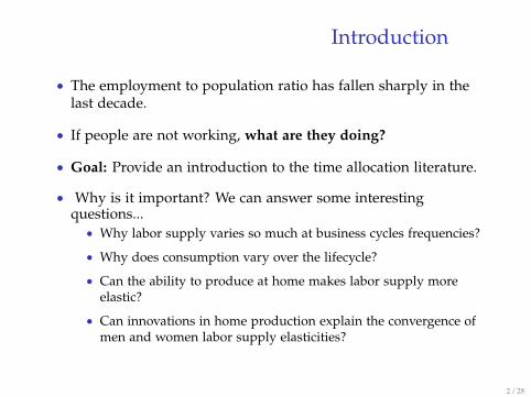
• The employment to population ratio has fallen sharply in thelast decade.
• If people are not working, what are they doing?
• Goal: Provide an introduction to the time allocation literature.
• Why is it important? We can answer some interestingquestions...
• Why labor supply varies so much at business cycles frequencies?
• Why does consumption vary over the lifecycle?
• Can the ability to produce at home makes labor supply moreelastic?
• Can innovations in home production explain the convergence ofmen and women labor supply elasticities?
2 / 28
Trends in Market Work
3 / 28
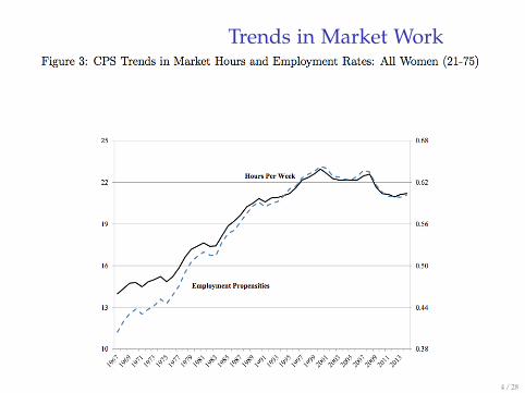
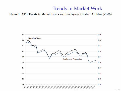
Trends in Market Work
4 / 28
Introduction
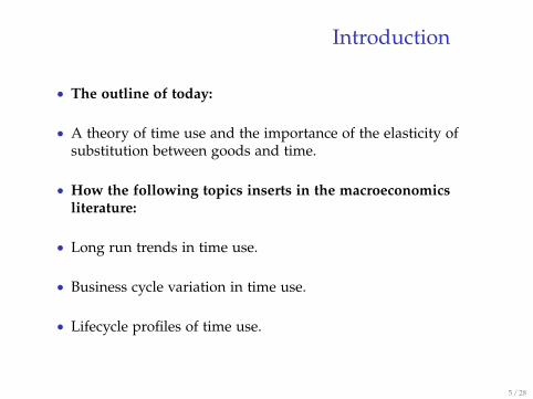
• The outline of today:
• A theory of time use and the importance of the elasticity ofsubstitution between goods and time.
• How the following topics inserts in the macroeconomicsliterature:
• Long run trends in time use.
• Business cycle variation in time use.
• Lifecycle profiles of time use.
5 / 28
Table of Contents
1 Introduction
2 A Theory of Time Use
3 Long Run Trends in Time Use
4 Business Cycle Variation in Time Use
5 Lifecycle Variation in Time Use
6 / 28
A Theory of Time Use
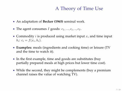
• An adaptation of Becker (1965) seminal work.
• The agent consumes I goods: c1, ..., ci, .., cI .
• Commodity i is produced using market input xi and time inputhi: ci = f(xi, hi).
• Examples: meals (ingredients and cooking time) or leisure (TVand the time to watch it).
• In the first example, time and goods are substitutes (buypartially prepared meals at high prices but lower time cost).
• While the second, they might be complements (buy a premiumchannel raises the value of watching TV).
7 / 28
A Theory of Time Use
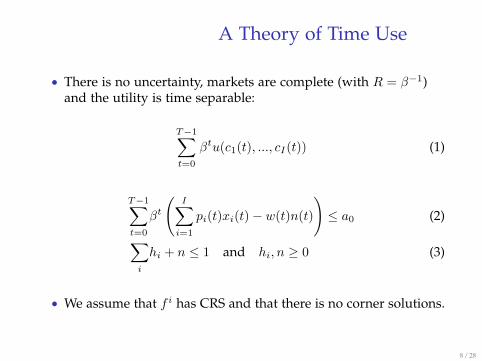
• There is no uncertainty, markets are complete (with R = β−1)and the utility is time separable:
T−1∑t=0
βtu(c1(t), ..., cI(t)) (1)
T−1∑t=0
βt
(I∑i=1
pi(t)xi(t)− w(t)n(t)
)≤ a0 (2)∑
i
hi + n ≤ 1 and hi, n ≥ 0 (3)
• We assume that f i has CRS and that there is no corner solutions.
8 / 28
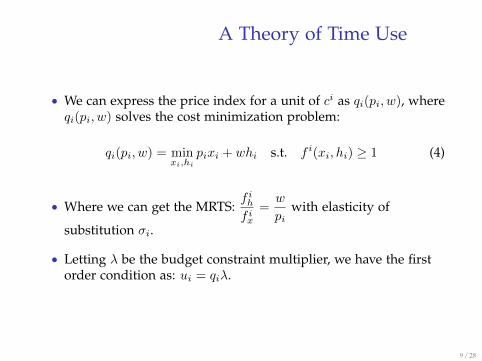
A Theory of Time Use
• We can express the price index for a unit of ci as qi(pi, w), whereqi(pi, w) solves the cost minimization problem:
qi(pi, w) = minxi,hi
pixi + whi s.t. f i(xi, hi) ≥ 1 (4)
• Where we can get the MRTS:f ihf ix
=w
piwith elasticity of
substitution σi.
• Letting λ be the budget constraint multiplier, we have the firstorder condition as: ui = qiλ.
9 / 28
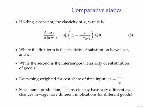
Comparative statics
• Holding λ constant, the elasticity of xi w.r.t w is:
d lnxid lnw
∣∣∣λ
= sih
(σi −
ui−uiici
)≶ 0 (5)
• Where the first term is the elasticity of substitution between xiand hi.
• While the second is the intertemporal elasticity of substitutionof good i.
• Everything weighted for cost-share of time input: sih =wh
qi.
• Since home-production, leisure, etc may have very different σi,changes in wage have different implications for different goods!
10 / 28
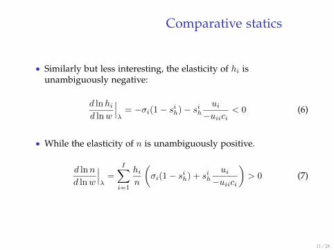
Comparative statics
• Similarly but less interesting, the elasticity of hi isunambiguously negative:
d lnhid lnw
∣∣∣λ
= −σi(1− sih)− sihui−uiici
< 0 (6)
• While the elasticity of n is unambiguously positive.
d lnn
d lnw
∣∣∣λ
=
I∑i=1
hin
(σi(1− sih) + sih
ui−uiici
)> 0 (7)
11 / 28
Table of Contents
1 Introduction
2 A Theory of Time Use
3 Long Run Trends in Time Use
4 Business Cycle Variation in Time Use
5 Lifecycle Variation in Time Use
12 / 28
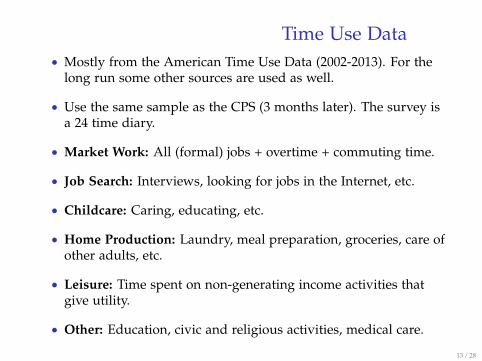
Time Use Data• Mostly from the American Time Use Data (2002-2013). For the
long run some other sources are used as well.
• Use the same sample as the CPS (3 months later). The survey isa 24 time diary.
• Market Work: All (formal) jobs + overtime + commuting time.
• Job Search: Interviews, looking for jobs in the Internet, etc.
• Childcare: Caring, educating, etc.
• Home Production: Laundry, meal preparation, groceries, care ofother adults, etc.
• Leisure: Time spent on non-generating income activities thatgive utility.
• Other: Education, civic and religious activities, medical care.
13 / 28
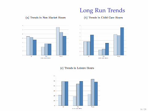
Long Run Trends
14 / 28
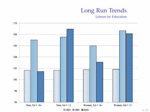
Long Run TrendsLeisure by Education
15 / 28
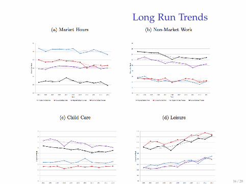
Long Run Trends
16 / 28
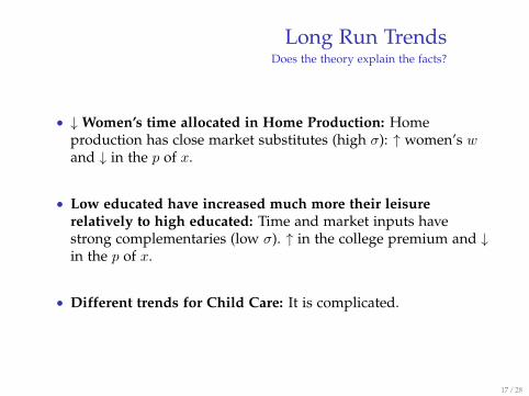
Long Run TrendsDoes the theory explain the facts?
• ↓Women’s time allocated in Home Production: Homeproduction has close market substitutes (high σ): ↑ women’s wand ↓ in the p of x.
• Low educated have increased much more their leisurerelatively to high educated: Time and market inputs havestrong complementaries (low σ). ↑ in the college premium and ↓in the p of x.
• Different trends for Child Care: It is complicated.
17 / 28
Table of Contents
1 Introduction
2 A Theory of Time Use
3 Long Run Trends in Time Use
4 Business Cycle Variation in Time Use
5 Lifecycle Variation in Time Use
18 / 28
Business Cycle Variation in Time Use
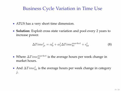
• ATUS has a very short time dimension.
• Solution: Exploit cross state variation and pool every 2 years toincrease power.
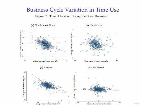
∆Timejjt = αj0 + αj1∆Timemarketkt + εjkt (8)
• Where ∆Timemarketkt is the average hours per week change inmarket hours.
• And ∆Timejkt is the average hours per week change in categoryj.
19 / 28
Business Cycle Variation in Time Use
20 / 28
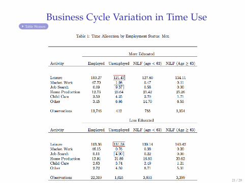
Business Cycle Variation in Time UseTable Women
21 / 28

Business Cycle Variation in Time UseMacroeconomics Implications
• Home production can improve the performance of DSGE inseveral dimensions.
• Volatility can arise because of differences in productivities of themarket and the home produced good.
• Relative prices changes cause households to substituteintratemporally, introducing a powerful amplificationmechanism.
• In a calibrated version of a RBC model, the introduction ofhome production:
• ↑ Volatility of labor and consumption.• ↓ Correlation of productivity and labor hours.
22 / 28
Table of Contents
1 Introduction
2 A Theory of Time Use
3 Long Run Trends in Time Use
4 Business Cycle Variation in Time Use
5 Lifecycle Variation in Time Use
23 / 28
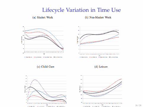
Lifecycle Variation in Time Use
24 / 28
Lifecycle Variation in Time UseMacroeconomics Implications
• In the usual model of lifecycle consumption, the PIH implieshouseholds smooth their consumption.
• The typical finding is that consumption follows a hump shaped(tracking labor income).
• Explanations: Poor planning, liquidity constraints, impatience...
• But there are strong heterogeneity in the expenditure patterns!• Some display the hump-shape (food, transportation).• Others increase (entertainment).• Others decrease (clothing, personal care).
25 / 28
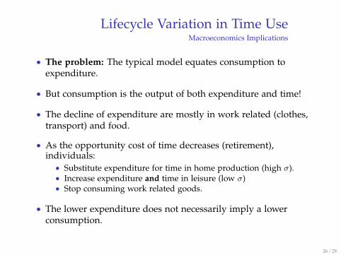
Lifecycle Variation in Time UseMacroeconomics Implications
• The problem: The typical model equates consumption toexpenditure.
• But consumption is the output of both expenditure and time!
• The decline of expenditure are mostly in work related (clothes,transport) and food.
• As the opportunity cost of time decreases (retirement),individuals:
• Substitute expenditure for time in home production (high σ).• Increase expenditure and time in leisure (low σ)• Stop consuming work related goods.
• The lower expenditure does not necessarily imply a lowerconsumption.
26 / 28
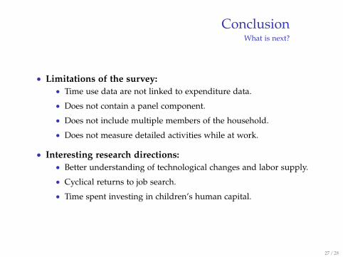
ConclusionWhat is next?
• Limitations of the survey:• Time use data are not linked to expenditure data.
• Does not contain a panel component.
• Does not include multiple members of the household.
• Does not measure detailed activities while at work.
• Interesting research directions:• Better understanding of technological changes and labor supply.
• Cyclical returns to job search.
• Time spent investing in children’s human capital.
27 / 28

Thank you!
28 / 28
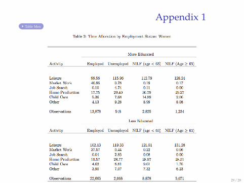
Appendix 1Table Men
29 / 28