Agricultural policy in an uncertain world

Agricultural policy in an uncertain world

Jean-Paul Chavas*

University of Wisconsin, Madison, USA

Received January 2011; final version accepted May 2011

Review coordinated by Thomas Heckelei

Abstract

This paper briefly reviews the current food situation and provides some historicalperspectives on its evolution over time. It documents the important effects of agricul-tural productivity. It also evaluates the role of externalities, uncertainty and policy inthe agricultural sector. The analysis stresses the joint role of uncertainty and extern-alities in the analysis of efficiency issues in the agricultural sector. Implications forfarm management and agricultural policy are discussed.

Keywords: agriculture, efficiency, technological change, uncertainty, policy

JEL classification: Q1, D6, D8

1. Introduction

The role of agriculture in the world is complex. While farming is in thebusiness of using agro-ecosystem services to feed people, it does so in differ-ent ways over time as well as across space. This paper briefly reviews thecurrent food situation and provides some historical perspectives on itsevolution over time. And it documents the important effects of agriculturalproductivity. It also evaluates the role of externalities, uncertainty andpolicy in the agricultural sector. But addressing all the complexities ofagriculture cannot be accomplished within a single paper. This means thatour analysis must be limited in scope. As a result, we focus only on asubset of the important issues facing agriculture today.1 In addition, ourdiscussion centres on agriculture in the USA and Europe.2

This paper focuses on the joint role of uncertainty and externalities in theanalysis of efficiency issues in the agricultural sector. Production uncertaintyis an important characteristic of agriculture: unpredictable factors such as

*Corresponding author: Taylor Hall, University of Wisconsin, Madison, WI 53713, USA. E-mail:

[email protected]

1 Some important issues we do not cover include food quality, food safety and the dynamics of

agro-ecosystem management.

2 Yet, many of the arguments presented in this paper appear relevant to agriculture around the

world.

European Review of Agricultural Economics pp. 1–25doi:10.1093/erae/jbr023

# Oxford University Press and Foundation for the European Review of Agricultural Economics 2011; all rightsreserved. For permissions, please email [email protected]

European Review of Agricultural Economics Advance Access published June 24, 2011 by guest on June 25, 2011

erae.oxfordjournals.orgD

ownloaded from

http://erae.oxfordjournals.org/

weather effects, diseases and pest damages can have large effects on farmoutputs. Agricultural markets can also be unstable, generating large pricevolatility that can be difficult to anticipate. This stresses the role of risk man-agement in the agricultural sector. In addition, agricultural productioninvolves using ecosystem services to produce food. The functioning ofagro-ecosystems is complex and involves significant interactions amongmany variables (water, nutrients, water, temperature, etc.). These interactionsoften take forms of externalities that need to be managed. Coase (1960) pro-posed an approach to identify the efficient management of externalities. Inter-estingly, he used interactions between crops and livestock to motivate hisanalysis. The last few decades have seen a rise in ecological concerns withimplications for agricultural management and policy. These concerns makeCoase’s analysis even more relevant today.

The paper is organised as follows. After presenting a broad overview of therecent history of agriculture, the paper documents advances in farm pro-ductivity as well as some challenges facing the food sector (in Section 2).This helps motivate the need to improve the management of both risk andexternalities in agriculture. An important contribution of the paper is toextend the Coasian approach to include risk allocation in efficiency evalu-ations (in Sections 3 and 4). Implications for farm management and agricul-tural policy are discussed in Section 5. Section 6 evaluates current andfuture challenges for the economics of agriculture and agricultural policy.

2. Historical perspectives

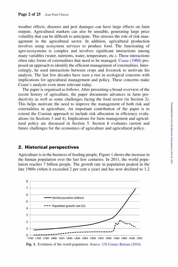
Agriculture is in the business of feeding people. Figure 1 shows the increase inthe human population over the last few centuries. In 2011, the world popu-lation reaches 7 billion people. The growth rate in population peaked in thelate 1960s (when it exceeded 2 per cent a year) and has now declined to 1.2

Fig. 1. Evolution of the world population. Source: US Census Bureau (2010).

Page 2 of 25 Jean-Paul Chavas

by guest on June 25, 2011erae.oxfordjournals.org

Dow

nloaded from


per cent a year. Yet, 1 billion people have been added over the last 11 years.Feeding the growing world population is a significant challenge.

This challenge has generated a debate involving two polar scenarios. On theone hand, increases in human population put pressure on natural resources andthe ability of the earth to provide food for all. This is the Malthusian scenario,which associates population increases with rising resource scarcity and thespread of famine. On the other hand, technological progress has greatlyincreased the productivity of land and labour. Under a positive feedbackfrom the size and density of human population to technological change, pro-ductivity growth can help deal with increased resource scarcity. This is theBoserupian scenario, which relies on induced innovations (Boserup, 1965,1981). The induced innovation hypothesis states that new technologies arelikely to develop and be adopted in response to changes in resource scarcity(Hicks, 1932; Binswanger, 1974; Ruttan, 2001; Acemoglu, 2002; Acemogluet al., 2009). For example, it means that increasing (decreasing) the cost ofa resource tends to stimulate the development and use of technologies thatreduce (increase) the use of this resource.

Agriculture provides a great case study of the induced innovation hypothesis.The rise of agriculture some 10,000 years ago appears consistent with inducedinnovations. As documented by Boserup (1965, 1981) and Kremer (1993), thehistorical evidence shows that the switch from hunting-gathering to agricul-ture did not take place without a rise in population density. The argument isthat farming requires more effort than hunting-gathering, implying that noindividual would want to switch from hunting-gathering to farming unlessthe former fails to provide enough food to satisfy human needs. This latterscenario develops when the human population rises beyond some thresholdwhere the ecosystem can no longer feed the human population throughhunting-gathering activities alone. It means that the historical rise of agricul-ture was an induced response to food scarcity associated with a rising popu-lation. This includes the cultivation of wheat and barley in Mesopotamia,starting around 8000 BC, of maize in Mexico and of rice in China startingaround 5000 BC (Heiser, 1990: 6–8).

2.1 Food prices

The evolution of food prices over the last decade is shown in Figure 2 for threeagricultural commodities: corn, wheat and rice. It shows very large changes infood prices in 2008. In a period of few months, food prices basically doubled,followed by a very sharp decline. The changes were most dramatic for rice.These rapid price fluctuations are quite unsettling for any market participant.Higher commodity prices benefit sellers (including grain farmers), but theyhurt buyers (including consumers, and dairy/livestock farmers who facehigher feed cost). Alternatively, lower commodity prices benefit buyers(including consumers), but they hurt sellers. While there are many factors con-tributing to such large price swings, this market instability makes anticipatingfuture price patterns very difficult. It means the presence of significant price

Agricultural policy in an uncertain world Page 3 of 25


Dow

nloaded from


risk/uncertainty for market participants. This puts a premium on developingmanagement and/or policy schemes that can help deal with this uncertainty.

A longer-term look at agricultural prices is given in Figure 3. It shows thereal price of food over the last century for three farm commodities: corn, milkand wheat. The prices are real US prices, defined as nominal prices divided bythe US consumer price index (normalised to equal 1 in 1983). By correctingfor inflation, these real prices give useful information on the evolving per-formance of agriculture in feeding the world. They show two importantcharacteristics. First, they exhibit a trend towards a long-term decline inreal prices. Over the last 90 years, the average annual rate of change in realprice was 21.8 per cent for corn, 21.9 per cent for wheat and 20.8 percent for milk. For consumers, this reflects a decline in the real cost of food.This is a remarkable fact: agriculture has been able to feed the growingworld population at a lower price for consumers. Second, Figure 3 exhibits

Fig. 2. Nominal prices of food, 2000–2010, USD per ton. Source: FAO (2010).

Fig. 3. Real prices of food, 1913–2010, USD 1983. Source: ERS, USDA (2010).



Dow

nloaded from


much variability in real prices over time. Two periods are particularly note-worthy: the 1930s (during the Great Depression) when food prices werevery low; and the early 1970s when food prices were very high. The 1970swas a period exhibiting high population growth and increased resource scar-city. But it was followed by three decades of fairly steady decline in real pricesfor food. While this may be good news for consumers, it raises the questionabout what is coming next.

2.2 Agricultural productivity

What is the main source of the long-term decline in real food prices? The shortanswer is: improvements in agricultural productivity. Figures 4 and 5 illustratethe evolution of agricultural yields over the last few decades. Figure 4 showshow US yields have changed for three commodities: corn, wheat and milk.Over the last 80 years, the average annual growth rate in yield was 2.0 percent per year for corn and 1.4 per cent per year for wheat, reflecting verylarge increases in land productivity. Similarly, the last 80 years have seenan average annual growth rate in milk production per cow of 1.9 per centper year. Figure 5 shows the evolution of yield for selected farm commoditiesin France. Like Figure 4, it shows a large and steady increase in land pro-ductivity over the last 50 years. Since 1930, the average annual growth ratein yield was 2.3 per cent per year for corn and 1.9 per cent per year for softwheat. These are very large increases that were crucial in increasing foodproduction.

How much of these increases come from technological change? Part of thehistorical increases in food production came from increased input use (e.g. fer-tiliser, pesticides, capital). But the evidence shows that most of these increasescame from technological improvements (Ball et al., 1997; Gardner, 2002;Fuglie, 2008). For example, Ball et al. (1997) documented that US agriculturalproduction grew at an average rate of 2 per cent annual rate over the last few

Fig. 4. Evolution of agricultural yields, USA, 1913–2010. Source: ERS, USDA (2010).



Dow

nloaded from


decades, most of it (1.94 per cent) coming from productivity growth (asmeasured by a total factor productivity TFP index). Remarkably, suchchanges took place while US agricultural labour input was declining at anaverage rate of 2.7 per cent a year (reflecting both rural–urban migrationand increased mechanisation). In addition, Fuglie (2008) found that, overthe last four decades, agricultural productivity has been growing at fairlyhigh rates in most regions of the world. This reflects the important roleplayed by innovations in farming systems, fertiliser use, pest controlmethods, mechanisation and genetic selection. It means that technologicalchange has been the principal factor responsible for increased food productionaround the world. And at this point, there is no strong evidence of a generalslowdown in agricultural productivity growth.

2.3 Some lessons from history

Agriculture has been associated with large increases in food production perhectare. Rising agricultural productivity has played a major role in improvingthe ability of agro-ecosystems to feed a growing world population. Yet,dealing with increased resource scarcity was not always easy. Historyreminds us that there were also difficult times. This includes the 1315–1317 great famine in Europe, the 1849–1850 Irish potato famine and the1958–1961 great famine in China (where 30 million people died of star-vation). This indicates that, while high population can stimulate technologicalprogress, it can also test the ability of the human race to sustain itself. Below,we reflect on these challenges through three historical examples: the Irish

Fig. 5. Evolution of agricultural yields, France, 1862–2007. Note: The figure is from

Agreste Primeur (2008). The yields are in quintals (100 kg) per hectare. ‘Maıs grain’ is

corn, ‘Orge’ is barley, ‘Ble tendre’ is bread wheat and ‘Ble dur’ is durum wheat.



Dow

nloaded from


potato famine, the near extinction of the North American buffalo and the DustBowl.

2.3.1 The Irish potato famine

The potato, a native of South America, was introduced in Ireland in the latesixteenth century. The following two centuries saw a rapid increase in its pro-duction and consumption in Ireland. By the early nineteenth century, potatowas the dominant staple in the diet of the Irish peasant class. This wasmade possible by a remarkable characteristic: potato is one of the very fewfoods that is high in calories, protein, minerals and vitamins (except for vita-mins A and D). As such, it can function as the main source of individual nutri-tion over an extended period of time (Davies, 1994). In addition, potatoproductivity was generally good: it could produce more nutrients on lessland than other crops (including wheat and corn). As a result, the early1800s saw Ireland solve its problem of feeding a growing population by plant-ing more potatoes, as both production and consumption became highlyspecialised in potato, especially for the Irish poor.

The great Irish famine was triggered in 1845 by a potato disease (the potatoblight) which destroyed nearly half of the potato crop. This was followed bycontinued widespread crop failures and food shortages in the following fewyears. During the period 1846–1850, the devastation led to 1 million Irishpeople starving to death, and as many others emigrating to the UK, theUSA, Canada and Australia.

The Irish potato famine was a tragedy of historical proportion. It stimulatedacademic interest in at least three directions. First, it documented the danger ofextreme forms of specialisation, especially in food systems that are subject tounanticipated production shortfalls. This is a lesson that remains valid today.Second, the Irish potato famine identifies the role of migration as an importantresponse to adverse shocks. Moving can provide an effective relief to peopleaffected by unforeseen adversity. But this raises the question: in situations ofadversity, to what extent would the migration option still be available today?Third, the Irish potato famine stimulated interest into the type of economic be-haviour that may arise during periods of distress. Of special interest has beenthe nature of subsistence-driven behaviour and its implications for fooddemand (e.g. Davies, 1994; Rosen, 1999). Could it be that potato was aGiffen good in Ireland, i.e. an inferior good with negative income effectsthat were strong enough to generate upward-sloping demand curve (Davies,1994)? There is the possibility that poor individuals would indeed exhibitGiffen behaviour. Could it apply also at the market level? This would indicatethat the price of potato could actually rise during a production shortfall, thusreducing the purchasing power of the poor and making the famine even worse.The empirical evidence does not support this hypothesis at the market levelduring the Irish potato famine (Rosen, 1999). Yet, the nature of consumptionbehaviour under situations of poverty and malnutrition remains of interest. Forexample, Jensen and Miller (2008) found evidence of Giffen consumption be-haviour among the poor in China. While the demand for food has typically



Dow

nloaded from


been found to be price inelastic, such inquiries indicate that the elasticity ofdemand of food may be even lower in situations of malnutrition. This isimportant since it would suggest that unanticipated supply shocks generatingfood shortfalls could also contribute to large price swings. This is one of thekey contributing factors to price instability in agricultural markets.

2.3.2 The near extinction of the North American buffalo

In the sixteenth century, there were about 25–30 million buffalos in NorthAmerica. By 1890, only about 100 remained wild in the US Great Plains.About 10–15 million were killed during a rather short period of time from1870 to 1880. This is one of the more notable environmental disasters inAmerican history. This slaughter did stimulate the implementation of US con-servation policies in the early twentieth century (e.g. the creation of the USNational Park system). But what caused it? Taylor (2007) has recently exam-ined the reasons for this conservation failure. He documents the economicfactors that contributed to this environmental disaster. He stresses three keyfactors: (i) open-access conditions in the Great Plains, with no regulation ofthe buffalo kill; (ii) technological progress in tanning that greatly stimulatedthe demand for buffalo hides; and (iii) free trade in the 1870s and 1880sand a very elastic demand in buffalo hides (mostly from Europe). The firstfactor stresses the importance of institutions and policy in resource manage-ment (e.g. Ostrom, 1990). The second factor reminds us that, while ingeneral beneficial, technological progress can have adverse effects onresource use. And the last factor indicates that, under some circumstances,free trade can contribute to resource depletion. In summarising the impli-cations of his analysis, Taylor (2007) writes:

The story of the buffalo has as much relevance today as it did 130 yearsago. Many developing countries in the world today are heavily reliant onresource exports, and few have stringent regulations governing resourceuse. The slaughter on the plains tells us that waiting for development tofoster environmental protection can be a risky proposition: In just a fewshort years, international markets and demand from high income countriescan destroy resources that otherwise would have taken centuries to deplete.

2.3.3 The Dust Bowl

The Dust Bowl was one of the most severe US environmental disasters of thetwentieth century. Severe drought followed by extreme levels of wind erosionhit the US Great Plains in the 1930s. Strong winds swept top soil in massivedust storms, reducing substantially the land’s potential for agricultural pro-duction. This ecological disaster was created by the interactions betweenadverse weather patterns and farm practices used.

Over the previous decades, grassland in the US Great Plains had beenploughed to plant wheat. When the rainfall was sufficient, this generatedgood yields which stimulated more settlements and cultivation. The droughtstarted in the early 1930s, generating crop failures. As the drought deepened,



Dow

nloaded from


the ground cover that held the soil in place disappeared, leaving the soilexposed to wind erosion. Starting in 1933, strong dust storms strippedtopsoil and blew it sometimes thousands of miles towards the Eastern USA,causing extensive damage. The catastrophic conditions stimulated a largemigration: by 1940, 2.5 million people had moved out of the US Great Plains.

What lessons can we learn from the Dust Bowl experience? First, we nowknow that farming practices used at the time were not sustainable. Hansen andLibecap (2004) have documented that externalities were involved: whilefarmers could prevent wind erosion by fallowing land or converting croplandinto grasslands, much of the benefits would be captured by neighbouringfarms. Such externalities were not well managed at the time, stressing theneed for the development of appropriate coordination and policy schemes.Second, the Dust Bowl showed the presence of significant interactionsbetween poor land conservation practices and adverse weather shocks: thesevere and prolonged drought exacerbated the effects of mismanagement,turning them into a full-scale disaster. Such interactions between unforeseenevents and poor environmental and resource management remain validtoday. Third, while the Dust Bowl stimulated the development of USconservation policies, its longer-term effects remain of interest (Hornbeck,2009). As noted above, an important effect was massive outmigration. Buthow important were the adjustments in agricultural land use? Hornbeck(2009) showed that such long-term adjustments in land productivity were ingeneral slow and partial, as they recovered only 14–28 per cent of theinitial decline. In this case, besides migration, local adaption to environmentaldestructions proved to be limited.

3. Economic efficiency

The above discussion has identified four important factors that influence theperformance of agriculture: technology, uncertainty, trade and environmentalexternalities. This section attempts to integrate these factors in the evaluationof efficiency.

3.1 Pareto efficiency

The concept of Pareto efficiency is well known in economics. It identifies allo-cations that maximise aggregate benefit across all individuals in society. Toillustrate, consider a society composed of S individuals. Following Luenberger(1995), define the benefit function of the sth individual as his/herwillingness-to-pay starting from a bundle of goods zs to reach a utility levelUs, s ¼ 1, . . ., S. Denote the corresponding aggregate benefit in society byB(z, U), where z ¼ (z1, . . ., zS) and U ¼ (U1, . . ., US). Let Z(T) be the feasible

set for∑S

s=1 zs, where T is a technology index and∑S

s=1 zs[Z(T) means that

aggregate goods∑S

s=1 zs can be produced under technology T. As shown by

Luenberger (1995), Pareto efficient allocations are allocations satisfying the



Dow

nloaded from


following two conditions: (i) V(U, T) ¼Maxz {B(z, U):∑S

s=1 zs[Z(T)}; and

(ii) choose a U that satisfies V(U, T) ¼ 0. The first condition is intuitive: itstates that Pareto efficiency implies maximising aggregate benefit. Thesecond condition states that once maximised, aggregate benefit V(U, T)must be totally re-distributed among the N individuals in society (with theset {U: V(U, T) ¼ 0} defining the Pareto utility frontier).

This simple characterisation is very general. It applies in a general equili-brium context, allowing for complex interactions/externalities across sectorsand economic agents (e.g. see Luenberger, 1995). It applies under uncertaintywhen one defines commodities to be ‘state-contingent’ (see Debreu, 1959;Chambers and Quiggin, 2000). It applies under any technology, includingtechnologies exhibiting non-convexity (Chavas and Briec, 2011). And itapplies with or without markets. While this is very nice, this characterisationhas two limitations: (i) it does not tell us how aggregate benefit should be dis-tributed among individuals in society; and (ii) it does not help us identify therole of markets versus non-market institutions. Both limitations are relevant inthe analysis of government policy.

The evaluation of market versus non-market institutions is a difficult one.We know that markets can generate Pareto efficient allocations under the fol-lowing conditions (Debreu, 1959): (i) no externality; (ii) convex technology;and (iii) complete and competitive markets. Then, market-clearing prices aresocial prices (measured as the aggregate benefit generated by one more unit ofthe corresponding goods), and efficiency is obtained under decentraliseddecision-making and free markets (including free trade). This generates twoimportant results. First, free trade can support an efficient allocation. Alterna-tively stated, trade liberalisation can generate efficiency gains (as furtherdiscussed below). Second, technological progress increases aggregatewelfare. Indeed, any improvement in technology from T to T ′, with Z(T) ,Z(T ′), implies a rise in aggregate benefit: V(U, T ′) ≥ V(U, T ). Note that thisdoes not say how the associated welfare gains get distributed in society.The issue of the distribution of benefits from technological improvements isrelevant in agriculture (as further discussed below).

Knowing that competitive markets can be efficient is useful. But this doesnot identify any role for government pricing policy. It suggests that govern-ment economic policy needs to be motivated in situations where some ofthe Debreu conditions are not satisfied and/or there are concerns aboutdistribution issues across individuals.3

3.2 Efficiency in agriculture

Below, we discuss efficiency in the agricultural sector. As motivated above,we focus on two important characteristics: the presence of externalities; andthe fact that risk is important in agriculture and risk markets are typically

3 See Chavas (2008) for an analysis of efficiency under fairness.



Dow

nloaded from


incomplete. Assuming that farmers are price-takers, our analysis proceeds atthe sector level, taking prices as given.4

Consider an agricultural sector involving Q farms.5 The Q farms are part ofa farming system in a given agro-ecological region. The qth farm uses N inputsxq ¼ (x1q, . . ., xNq)′ to produce M outputs yq ¼ (y1q, . . ., yMq)′. Let x ¼ (x1, . . .,xQ) and y ¼ (y1, . . ., yQ). Let e be a vector of random variables representingproduction uncertainty, and let T be a technology index. The production possi-bility set of the agro-ecosystem is represented by F(T, e), where (x, y) [ F(T,e) means that inputs x can produce outputs y under technology T and state e.Because of production lags, we assume that inputs are chosen ex ante, whileoutputs are chosen ex post. This means that, while the choice of xq does notdepend on e, our discussion below implicitly allows the choice of yq todepend on e. Note that the feasible set F(T, e) is quite general: it allows forproduction uncertainty and any technology, including possible productivityinteractions among outputs as well as externalities across farms. It will be con-venient to represent the underlying technology by the aggregate productionfunction

f (x, y2:M, T, e)= Maxy1

∑q

y1q : (x, y) [ F(T, e){ }

if a maximum exists,

= −1 otherwise,

(1)

where y1 ¼ (y11, . . ., y1Q) and y2:M ¼ {(y2q, . . ., yMq): q ¼ 1, . . ., Q}. Let

(y+11(x, y2:M, T, e), . . . , y+1Q(x, y2:M, T, e))[ argmax{y1q}{∑

q y1q: (x, y)[F(T,

e)} in the maximisation problem (1), with f (x, y2:M, T, e) =Sqy+1q(x, y2:M, T, e). Given (x, y2:M, T, e), equation (1) defines f(x, y2:M, T, e)

as an aggregate stochastic production function measuring the largest possibleaggregate quantity of the first output, where feasibility (x, y) [ F(T, e) impliesthat

∑q y1q ≤ f(x, y2:M, T, e). In addition, assuming that the maximisation in

equation (1) has a unique solution, y+1q(x, y2:M,T, e) can be interpreted as a

stochastic production function for the qth farm, q ¼ 1, . . ., Q. Again, this pro-vides a generic representation of the technology, allowing for productionuncertainty and possible productivity interactions among outputs as well asexternalities across farms.

The agricultural sector is part of a market economy where inputs x andoutputs y are market goods. We assume that each of the Q farms is a family

4 Focusing on a single sector makes the analysis simpler (compared with a general equilibrium

approach assessing the allocation and prices in all sectors). Taking prices as given means that

our analysis of efficiency would remain valid provided that prices are social prices. Note that

this neglects issues related to price inefficiency (when prices depart from social prices).

5 By focusing on the farm sector, our analysis can address the management of externalities

among farms. When the externalities go beyond the farm sector, the analysis would need to

be extended to include all economic agents affected by the externalities.



Dow

nloaded from


farm where the owner, the manager and the farm worker are the same person,i.e. where there is no separation of ownership and control. Let p ¼ (p1, . . .,pM) . 0 be the vector of uncertain prices for outputs, and r ¼ (r1, . . ., rN)be the vector of input prices.6 Letting wq be exogenous income, denote thenet income of the qth farm by pq ; wq + p′yq 2 r′xq. Under incompleterisk markets, assume that each farmer maximises expected utility. For theqth farmer, this is denoted by EqUq(pq), where Eq is the expectation operatorbased on the subjective probability distribution of (p, e) reflecting the infor-mation available at decision time,7 and Uq(pq) is a utility function represent-ing the farmer’s risk preferences.8 Under non-satiation, we assume that Uq(pq)is a strictly increasing function.

For the qth farmer, define the certainty equivalent as the sure amount ofmoney CEq(xq, yq, .) satisfying

EqUq(pq) = Uq(CEq), (2)

where q ¼ 1, . . ., Q. Equation (2) shows that the certainty equivalent CEq(xq,yq, .) provides a general welfare measure for the qth farmer, where ‘.’ denotesother arguments (such as prices, risk preferences, risk exposure, etc.). Inaddition, under non-satiation, it implies that maximising EqUq(pq) is equival-ent to maximising the certainty equivalent CEq(xq, yq, .). We want to charac-terise an efficient allocation in situations that include both uncertainty andpossible externalities across farms. Following Coase (1960), this can bedone by maximising the aggregate welfare of all Q farmers:

W(T, ·) = Maxx,y

∑q

CEq(xq, yq, ·) : (x, y) [ F(T, e){ }

. (3)

Assuming the maximisation in equation (1) has a unique solution, equation (3)can be alternatively written as (see the proof in the appendix):

W(T, ·) = Maxx,y

∑q

CEq(xq, y+1q(x, y2:M,T, e), y2:M,q, ·){ }

, (4)

where W(T, .) is an aggregate welfare measure for the Q farmers under tech-

nology T. Equation (4) shows that the production functions {y+1q(x, y2:M, T, e):

6 As noted above, the analysis treats the prices (p, r) as given. For market goods under compe-

tition, these prices are treated as market equilibrium prices. In situations where (y, x) include

non-market goods, p would denote the marginal benefit of y, and r would denote the marginal

cost of x.

7 Note that we allow for active learning where the qth farmer’s subjective probability distribution

of (p, e) can depend on information-gathering activities in xq. This active learning can vary across

farmers.

8 For simplicity, we assume that income is the only source of utility for farmers. Note that the

analysis could be extended to include other arguments in the utility function (e.g. leisure,

environmental quality).



Dow

nloaded from


q ¼ 1, . . ., Q} summarise all the relevant information about the stochastic pro-duction technology. Letting p ¼ (p1, p2:M), which means that the certaintyequivalent CEq in equation (2) can be alternatively written as

CEq(xq, y2:M,q, T, ·) = U−1q EqUq[wq + p1y+

1q(x, y2:M, T, e) + p′

2:My2:M,q

− r′xq], (2′)

where q ¼ 1, . . ., Q.Following Pratt (1964), the implicit cost of risk for the qth farmer can be

measured by the Arrow–Pratt risk premium Rq(x, y2:M, T, .) defined as thesure amount of money Rq satisfying

CEq(xq, y2:M,q, T, ·) ; Eq[wq + p1y+1q(x, y2:M,T, e) + p′2:M

y2:M,q − r′xq]− Rq, (5)

where CEq(xq, y2:M, q, T, .) is defined in equation (2′). The risk premium Rq(x,y2:M, T, .) is the smallest sure amount of money the qth farmer is willing to payto replace the random income pq by its mean Eq(pq). We assume that eachfarmer is risk averse, where Uq(.) is a strictly concave function and the costof risk is positive: Rq(x, y2:M, T, .) . 0, q ¼ 1, . . ., Q.

Substituting equation (5) into equation (4) and using

f (x, y2:M,T, e) = Sqy+1q(x, y2:M, T, e) yield

W(T, ·) = Maxx,y

{Eq

[∑q

wq + p1f (x, y2:M,T, e)

+ p2:M

(∑q

y2:M,q

)− r

(∑q

xq

)]−∑

q

Rq(x, y2:M, T, ·),}

(4′)

which has solution (x*, y*). W(T, .) in equation (4′) is an aggregate welfaremeasure of production decisions under risk (including both price andproduction risk). It identifies efficient decisions that maximise the aggregatecertainty equivalent of all farmers, allowing for uncertainty and externalities.It includes two terms: aggregate expected profit,

∑q Eq(pq), minus the

aggregate cost of risk as measured by∑

qRq.

4. Assessing agricultural efficiency

4.1 The role of expected profit

The maximisation of aggregate expected profit in equation (4′) is a standardpart of economic analysis. First, it stresses the role of technical efficiency.Indeed, equation (4′) implicitly assumes that y1 ¼ f(x, y2:M, T, e), or equiva-

lently that y1q = y+1q(x, y2:M, T, e), q ¼ 1, . . ., Q. It means that efficient



Dow

nloaded from


decisions must be made in such a way that inputs and outputs are located onthe upper bound of the production possibility set, i.e. on the production fron-tier. Any decision that does not satisfy this condition would be deemed tech-nically inefficient.

Second, expression (4′) applies under externalities. This is reflected in the

production function f (x, y2:M,T, e) =∑

q y+1q(x, y2:M,T, e), showing that

the stochastic production function for the qth farm, y+1q(x, y2:M,T, e), can

depend on the inputs and outputs of other farms, (xq′, y2:M, q′), for q′= q.

This allows for positive as well as negative externalities among farms

(depending on whether y+1q(x, y2:M, T, e) is positively or negatively affected

by (xq′, y2:M, q′) for q′= q). Importantly, in the presence of externalities,

equation (4′) shows that the expected profit of all farms affected by external-ities become relevant in making efficient decisions. Doing so is crucial to‘internalise’ the externalities and to achieve an efficient allocation (Coase,1960). Alternatively, failing to do would generate an inefficient allocation.This stresses that efficiency requires some coordination scheme among allfarms affected by the externalities. As noted by Coase (1960), this can beachieved through private contracts among the affected parties. Interestingly,in the paper that earned him the Nobel Prize, Coase (1960) used theexample of a farmer and a cattle-raiser, where the externality comes fromstraying cattle that destroy the farmer’s crops. This may work well whenthe number of affected farmers is small. But when the number of farmersbecomes large, the private contracting solution may become difficult toimplement (e.g. because of economies of scale in obtaining and processinginformation about the externalities). Then, the required coordination schememay come from government policy. In this case, government policy wouldtry to manage the externalities in a way consistent with equation (4′). Import-antly, externalities imply that decentralised decision-making would be ineffi-cient. Indeed, equation (4′) shows that the maximisation of the qth farmer’sexpected utility can be efficient only in the absence of externalities (when

the qth farm stochastic production function becomes y+1q(xq, y2:M,q,T, e).Our analysis started from a characterisation of technology at the aggregate

level. By allowing some farms to produce nothing, it implicitly treats thenumber of active farms as endogenous. This means that equation (4′) canalso be used to evaluate the efficient structure of agriculture. Yet, the presenceof externalities across farms depends on the identity of each farm. Forexample, if an externality (either positive or negative) exists between twofarms, then a merger between these two farms would basically make thisexternality disappear. By internalising the externality under a single manage-ment, this would eliminate the need for a coordination scheme between thetwo farms. Does that mean that a merger would always be a desirable solutionto an externality problem? Not necessarily. This would depend on the qualityof management in the merged farm versus the quality of a coordinationscheme implemented between the two original farms. There are three possiblescenarios. First, if the quality of management in the merged farm is excellent,



Dow

nloaded from


then merger would be an efficient solution implemented in market economyunder a decentralised system. This is the ‘market solution’. Second, if thequality of coordination implemented between the two original farms is excel-lent, then private contracts between the two farms would provide an efficientsolution to the externality. This is the ‘contract solution’ applied to the originalfarm structure, where the terms of the contract correspond to a ‘Coasianbargain’ consistent with equation (4′). Third, if many farms are involvedand a contract solution proves difficult to implement, then agriculturalpolicy may provide an efficient solution to the externality problem. This isthe ‘government solution’.

Choosing between a market solution, a contract solution and a governmentsolution can be challenging. Proponents of either the market solution or thecontract solution typically point to the difficulties facing government agenciesin developing refined coordination schemes among many agents (difficultiesoften referred to as ‘government failures’). But such difficulties may also bepresent no matter what solution is proposed. In the context of contracts,these difficulties typically take the form of ‘incomplete contracts’ that limitthe effectiveness of coordination between the interested parties, thusmaking contracts a less attractive option. And when externalities involvemany farms, the merger solution may not be attractive for two reasons.First, it could lead to a very concentrated industry, which may no longerhave a competitive structure. Second, in the presence of extensive external-ities among many farms, the manager of merged farms would likely befacing the same difficulties as a central planner. He/she may then fail to inter-nalise the former externalities, in which case technical and/or allocative inef-ficiencies would arise as his/her decisions differ from equation (4′). Suchdifficulties applied to either the market solution or the contract solution areoften referred to as ‘market failures’. In all cases, the issue focuses its attentionon the managerial abilities of the decision-makers as reflected by their abilitiesto obtain and process information about the relevant externalities.9 Goodfarm-level access to information is necessary to support a decentralisedscheme (in either the market solution or the contract solution). Alternatively,the presence of economies of scale in acquiring and using information mayfavour more centralised schemes (including government policy). Choosingthe appropriate solution to an externality problem should be guided bywhich institution comes closest to satisfying equation (4′).

The above discussion makes it clear that the presence of externalitiesdepend on the definition of each farm and its boundary. This indicates thata narrow focus on externalities appears misplaced. Agriculture is in thebusiness of using agro-ecological systems to produce food. These systemsare complex as the production of food involves significant interactionsamong solar energy, plants, soil, water, pest populations and other factors.These interactions exist at all levels: at the plot level, at the farm level, at

9 Recall that our model allows for active learning by each farmer, with possible heterogeneity in

acquiring and using information across farms.



Dow

nloaded from


the regional level and at the earth level. To illustrate, at the plot level, there areproductivity gains from crop rotation (that helps keep pest population down).At the farm level, there are productivity gains from crop diversification (thateases bottleneck in labour demand during planting and harvesting) and fromcrop-livestock integration (as the use of manure improves soil productivity).At the regional level, there are productivity gains from preventing soilerosion or from establishing irrigation networks. And at the world level,there are productivity gains from identifying local plants and animals thatcan be used (possibly in other parts of the world) to help feed a growing popu-lation. This stresses the need to assess the performance of agriculture at aglobal level, including its effectiveness in using agro-ecological services inproducing food. Yet, many decisions are made at the farm level. Expression(4′) shows how both local and global levels are relevant. It means that themanagement of agro-ecological services is also important at the farm level,as farm managers face the challenge of managing agro-ecological servicesand their local interactions. The efficient management of these interactionsgenerates farm-level economies of scope. How good are farmers at managingtheir local agro-ecosystems? It depends in part on farmers’ managerial abil-ities. The fact that agriculture has evolved to transform and dominate manyecological systems around the world is an indication of the relative successof farming practices. Yet, this does not mean that current practices arenecessarily efficient. More empirical work is needed to evaluate theseissues and to identify improved management strategies for farming systems.

4.2 The role of risk

Expression (4′) also shows that the aggregate cost for risk∑

qRq is subtractedfrom expected profit. Going beyond the analysis presented by Coase (1960),this makes it clear that the cost of risk should be included in efficiency analy-sis. It stresses the welfare effects of risk exposure among risk-averse farmers.In general, an efficient allocation should try to reduce the aggregate cost ofrisk. This can be done in at least three ways. First, the qth farmer wants totake actions (xq, yq) to reduce his/her risk exposure. This can take the formof increasing the use of inputs that are ‘risk decreasing’ (e.g. irrigation orpest control, where ∂Rq/∂xiq , 0) and decreasing the use of inputs that are‘risk increasing’ (e.g. fertiliser, where ∂Rq/∂xiq . 0). This can also take theform of diversification schemes that can be an integral part of an efficient allo-cation when they contribute to reducing risk exposure. Second, the cost of riskfor the qth farmer, Rq(x, y2:M, T, .), can depend on the actions of his neigh-bours, (xq′, y2:M, q′) for q′ = q). In this case, the qth farmer’s risk exposureinvolves an externality that needs to be managed. As discussed above, shortof merger, its efficient management requires implementing coordinationschemes among the affected parties (using contracts and/or governmentpolicy). Third, the aggregate cost of risk

∑qRq in equation (4′) can be

reduced through risk-transfer mechanisms. By re-distributing the risk away



Dow

nloaded from


from the individuals that face a high cost of risk (as measured by Rq),10 suchmechanisms can reduce the aggregate cost of risk and are an integral part ofimplementing an efficient allocation of risk.11 This can be done using privateinsurance schemes, risk markets (e.g. hedging on futures markets) and/or gov-ernment policy. Each of these institutions has been involved re-distributingrisk in the agricultural sector. In the USA, the role of agricultural policy inrisk re-distribution started during the Great Depression (e.g. price support pro-grammes which reduce price risk were first put in place in the 1930s whenfarm income was low and price volatility was high). The role of agriculturalpolicy in re-distributing risk continues to this day (e.g. disaster payments, orthe subsidisation of crop and income insurance) (Gardner, 2002; Peterson,2009). Given the extensive price risk and production risk found in agriculture,a significant puzzle remains: agricultural insurance markets remain uncom-mon without extensive government subsidies. Why? This seems to reflectboth market failures (as agricultural insurance markets have been slow todevelop) and government failures (from the apparent need for large subsidies).Yet, over the last few decades, new risk management tools have developed inthe financial sector. In particular, the increasing availability of option con-tracts related to price risk and weather risk has created new opportunitiesfor risk management in agriculture.

5. Assessing technological change

Besides characterising efficiency, expression (4′) also shows how the technol-ogy index T affects welfare W(T, .). Consider the effects of a small change inT. Under differentiability, applying the envelope theorem to expression (4′)gives

∂W

∂T= E p1

∂f

∂T

( )[ ]− ∂(SqRq)

∂T, (6)

evaluated at the optimal x* and y*. When f . 0, this can be alternativelywritten as

∂W

∂T= E ( p1f ) ∂ln(f )

∂T

[ ]− ∂(SqRq)

∂T. (6′)

Consider the case where T represents time. Then, for a given e, it follows that∂ ln(f)/∂T is the rate of technological change (measured at the aggregate level)

10 In our model, risk re-distribution would take place by treating exogenous income, wq in equation

(4′), as state dependent.

11 Note that risk preferences can introduce income effects in the evaluation of the cost of risk. In

particular, following Pratt, under decreasing absolute risk aversion, the risk premium Rq

would decline with income wq, meaning that any income re-distribution would typically affect

both the cost of risk and production decisions in equation (4′). This is a scenario where income

distribution issues are no longer separable from efficiency considerations.



Dow

nloaded from


from one time period to the next. It measures the rate of change in aggregateoutput

∑qy1q due to a change in T. For given prices, equation (6′) evaluates

the welfare effects of technological progress in a simple and intuitive way.It shows that welfare change (∂W/∂T) is increasing with productivity gains(as measured by the rate of technological change, ∂ ln(f)/∂T). It also showshow welfare change (∂W/∂T) is impacted by risk: positively if ∂(

∑qRq)/

∂T , 0 (i.e. if technological change reduces the aggregate cost of risk); butnegatively if ∂(

∑q Rq)/∂T . 0 (i.e. if technological change increases the

aggregate cost of risk). Note that these results are very general: they applyunder any risk preferences, any risk exposure (with both price risk and pro-duction risk) and any technology. They point out that technological changecan help reduce the cost of risk (e.g. the case of breeding drought-resistantvarieties).

Expression (4′) identifies the optimal supply decisions. For the qth farm,denote the supply decisions by y∗q(T, e, ·), which in general depend on the

technology index T, q ¼ 1, . . ., Q. In a market economy, it means that Talso affects prices. Here we focus our attention on the effects on outputprices p.12 Denote the corresponding aggregate supply functions by

YS(T, e, ·) ; Sqy∗q(T, e, ·). And let YD(p, .) denote the aggregate excess-

demand for outputs.13 The market prices p*(T, e, .) are then the prices p satis-fying the market equilibrium conditions:

YS(T, e, ·) = YD( p, ·). (7)

When an increase in T stimulates aggregate supply (∂YS/∂T . 0) and whendemand functions are downward sloping, equation (7) implies that the techno-logical progress is associated with a decrease in prices p*: ∂p*/∂T , 0. Thismeans that consumers benefit from technological progress. And this impactbecomes stronger (weaker) when the demand function YD is less (more)responsive to price. Note that similar arguments apply to the effects of pro-duction uncertainty e: unanticipated production shocks would have a stronger(weaker) effect on market equilibrium prices p*(T, e, .) when the demandfunction YD is less (more) responsive to price.

In this context, the market equilibrium aggregate welfare of farmers is

W∗(T, ·) ; W( p∗(T, ·),T, ·). (8)

Under differentiability and using equation (6′), the welfare effects of

12 For simplicity, we assume that input prices are constant, i.e. input markets face an infinitely elas-

tic supply.

13 In local markets, YD would just be the demand from local markets. Alternatively, in global mar-

kets, YD would be the aggregate excess demand from the rest of the world.



Dow

nloaded from


technological change are given by

∂W∗

∂T= E ( p1f ) ∂ ln(f )

∂T

( )[ ]− ∂(SqRq)

∂T+ ∂W

∂p

( )∂p∗

∂T

( ). (9)

The first two terms in equation (9) are the effects given in equation (6′): theproductivity effect E[(p1 f) (∂ ln(f)/∂T)] minus the risk effect ∂(

∑q Rq)/∂T.

The last term is the market equilibrium effect associated with the inducedadjustment in prices p. In general, we expect (∂p*/∂T) , 0 as technologicalchange typically stimulates supply. It means that, while technological pro-gress tends to benefit consumers, its induced price effects tend to reduce pro-ducers’ welfare. Thus, at the aggregate level, farmers gain from technologicalprogress (∂W*/∂T . 0) when the productivity gain E[(p1 f) (∂ln(f)/∂T)] is largeand the induced price effect [(∂W/∂p) (∂p*/∂T)] is small. But farmers can losefrom technological progress (∂W*/∂T , 0) when the induced price effect[(∂W/∂p) (∂p*/∂T)] is negative and large. As noted above, this can happenwhen the demand function YD exhibits a low responsiveness to price. Sincethe demand for food typically exhibits a low elasticity of demand, this is alikely scenario for agriculture. It means that, while technological progresscan generate large benefits to consumers and society in general, farmers canactually be made worse off by adopting a new technology. This is a peculiarcharacteristic of food markets: through induced price adjustments, they canre-distribute the benefits of technological progress in a way that does notreward the agents that implemented it in the first place.

6. Assessing agricultural policy

The last few decades have seen a move towards increased trade in globalmarkets. Interestingly, market globalisation is not new. A wave of market glo-balisation took place in the period of 1860–1914, led by Great Britain(Frieden, 2006: 28–55). While Great Britain implemented mostly protection-ist trade policies during the industrial revolution (Chang, 2008: 40–48), itpushed for trade liberalisation in the late nineteenth century. This includedthe 1846 repeal of the British ‘Corn Laws’ (which protected British wheatprices from international competition). In the following decades, GreatBritain reduced tariff barriers and stimulated the development of globalmarkets for many commodities (including agricultural commodities). Thisglobalisation period basically ended with World War I. The period betweenWorld War I and World War II was characterised by growing protectionismaround the world and economic difficulties (including the Great Depressionof the 1930s). The current period of globalisation started in 1945 and wasled by the USA. The last five decades have seen a move towards reducingtrade barriers, rapid economic growth and an increasing importance of inter-national trade (Frieden, 2006: 39–55). The reduction in trade barriers wasfacilitated by bilateral free trade agreements (FTA) and international insti-tutions such as the World Trade Organization (WTO). But this time,



Dow

nloaded from


agriculture was not part of this trend. Indeed, protectionist trade policiesremain common in agriculture (using import tariffs, import quotas and/orexport subsidies). The resistance to reducing trade barriers in agriculturehas come from the USA as well as Europe. This was at the heart of thefailure of recent WTO trade negotiations. Yet, countries like Brazil andIndia have pushed for trade liberalisation in agricultural markets. Forexample, Brazil would gain from being able to export sugar to the currentlyprotected European and US markets.

This raises the question: what are the benefits of trade liberalisation? Econ-omic theory shows that trade generates aggregate efficiency gains. The argu-ments date back to Adam Smith and Ricardo, who argue that protectionistpolicies can retard economic growth by preventing productivity-enhancingspecialisation in global markets. Setting aside risk issues, there is a generalconsensus that specialisation can contribute to increased productivity.

While this identifies economic gains from globalisation, two questionsremain. First, how large are the benefits from market liberalisation and global-isation? And second, how are these benefits distributed? Economic models oftrade have shown that the aggregate benefits of trade are positive and in therange of 2–3 per cent of GDP (Bhagwati, 2002: 33). Compared to the pro-ductivity gains discussed earlier, these benefits appear relatively small. Itseems that a few years of technological change can generate greater aggregatebenefits than trade liberalisation. But the aggregate impacts of trade policyoften hide large distributional impacts. Trade typically generates gainersand losers. And in the absence of compensations for the losers, somegroups can benefit significantly from trade policy. In general, producers inexporting countries gain from trade liberalisation. Alternatively, producersin importing countries gain from trade restrictions. As producer groups tendto be well organised politically, these distributional effects seem to bedriving the political economy of trade policy: trade liberalisation is typicallyfavoured for commodities that a country exports, while protectionist policy isfavoured for commodities that a country imports. In the latter case, distribu-tional effects may well motivate trade restrictions, while efficiency-lovingeconomists lament that protectionist policies often amount to rent-seeking be-haviour by producer groups with adverse effects on aggregate efficiency.

Other issues related to agricultural policy are: How extensive is agriculturalpolicy? And what is its cost to society? In developed countries, agriculturalpolicy is extensive. Besides trade policy (discussed above), domestic policyinvolves large government subsidies to the farm and food sector [includingsubsidies on a number of inputs and outputs, price support programmes andincome support; see Gardner (2002), Peterson (2009) and OECD (2010)].Peterson (2009: 105–116) reports that the annual cost of agricultural policyaround the world amounts to USD 365 billion a year, or USD 1 billion perday. Most of this cost comes from high farm subsidies in developed countries,especially the EU (USD 153 billion a year), the USA (USD 100 billion a year)and Japan (USD 45 billion a year). That is a lot of money. One must surelywonder whether this is money well spent.



Dow

nloaded from


One argument is that agricultural policy is mainly to support the income offamily farms in developed countries. Indeed, agricultural policies in the USAand Europe were put in place during periods of important rural–urbanmigrations, when the average income of rural households lagged significantlybehind their urban counterparts. Also, as noted above, technological progressin agriculture greatly benefited urban households (in the form of lower foodprices) with possible adverse effects on farmers’ income. In this context,farm subsidies in developed countries could be seen as an incomere-distribution scheme from high-income urban households towards lower-income rural households. This characterisation may have been fairly accurate40 years ago. But it appears less accurate today. For example, Gardner (2002)has documented the evolution of the income distribution in the USA over thelast century. He found that the income gap between urban and rural house-holds in the USA has greatly diminished over the last two decades. Itmeans that, on average, the income of rural households has basically caughtup with the income of their urban counterparts. Interestingly, this is true forlarge farms as well as small farms: while small farm households still havelower average farm income, their increased reliance on off-farm incomeallowed them to make up the difference (Gardner, 2002: 339–349). Thisdocuments a rising and more equally distributed standard of living for USfarm households. This is a very positive aspect in the performance of US agri-culture. But the disappearing income gap between urban and rural householdsraises renewed questions about the political justifications for current farmsubsidies.

Finally, we may want to evaluate the performance of agriculture in terms ofits effects on consumer welfare. On this point, the overall evaluation must bepositive (e.g. Gardner, 2002: 339–343). As discussed above, the increasedavailability of food at a lower real price is a significant achievement of agri-culture over the last few decades. Most of this is due to rapid technologicalchange and strong productivity growth. The social benefits from productivityimprovements appeared to have dominated the overall performance of theagricultural sector.

7. Challenges for the future

Over the last few decades, agriculture has been characterised by high and sus-tained productivity growth. Overall, this is an amazing achievement to helpmeet the increased demand for food (as fuelled by population growth).What about the future? The recent developments in biotechnology offergood prospects for continued technological progress. Hopefully, agriculturalinnovations will come fast enough to deal with current and future resourcescarcity. Yet, significant challenges lie ahead.

Rising concerns about climate change indicate that the next few decadeswill see significant changes in agriculture around the world. Changing patternsin rainfall and temperature will be good for agriculture in some regions butbad in others. Weather uncertainty will likely increase. How will people



Dow

nloaded from


adjust? Improved agricultural technology and improved management canhelp. This stresses the need for refined risk management schemes at alllevels: the farm level, the national level and the international level. Yet, weshould be careful not to overestimate our ability to adjust to unforeseenadverse events. First, migration options will likely not be as effective asthey were in the past (e.g. as in the case of the Irish potato famine or theDust Bowl). Second, without migration, adjusting to persistent shocks mayprove difficult (e.g. as evidenced by a slow adaptation to the long-termeffects of the Dust Bowl). Mitigating the effects of climate change maywell be one of the most important challenges for agriculture in the twenty-firstcentury.

Also, rising concerns about environmental issues are and will continue toreshape agriculture and agricultural policy. These issues are at all levels:local, regional and global. At the local level, our analysis stresses that farmmanagers are in the business of managing their local agro-ecosystem. Itmeans that solutions to environmental issues must involve farmers. Alterna-tively, for environmental issues that are global, agricultural policy mustplay a role and be an integral part of broader environmental policy.

Sustainability issues are also on the rise. Our analysis has focused on a staticanalysis. Sustainability is about preserving the future. This identifies the needto introduce dynamics in our analysis. Combining markets and governmentpolicies will be needed. This will require refining our understanding of thedynamics of agro-ecosystems and of the long-term effects of current farmmanagement practices.

Finally, addressing emerging issues in agriculture will require refinedempirical research. We need to continue the evaluation of agricultural technol-ogy and its effects on resource scarcity and environmental management. Moreresearch is required to improve our understanding of how environmentalservices get transformed into supporting and feeding the human race. Thisincludes estimating the economic value of multifunctionality in agriculture.We need refined analyses to assess risk exposure (especially exposure tounfavourable events) and to evaluate the associated cost of risk. This iscrucial to improve risk management in agriculture at all levels, includingrefinements in agricultural policy. Finally, we need empirical investigationsof the resilience of agro-ecosystems as they adjust in a changing world.

Acknowledgements

I would like to thank two anonymous reviewers for useful comments on an earlier draft of the

paper.

References

Acemoglu, D. (2002). Directed technical change. Review of Economic Studies 69:

781–810.



Dow

nloaded from


Acemoglu, D., Aghion, P., Bursztyn, L. and Hemous, D. (2009). The environment and

directed technical change. NBER Working Paper No. 15451. Cambridge, MA: National

Bureau of Economic Research.

Agreste Primeur (2008). La Statistique Agricole, Numero 210. Montreuil-sous-Bois,

France: Service Central des Enquetes et Etudes Statistiques, Ministere de l’Agriculture

et de la Peche.

Ball, V. E., Bureau, J. C., Nehring, R. and Somwaru, A. (1997). Agricultural productivity

revisited. American Journal of Agricultural Economics 79: 1045–1063.

Bhagwati, J. (2002). Free Trade Today. Princeton, NJ: Princeton University Press.

Binswanger, H. P. (1974). A microeconomic approach to innovation. Economic Journal

84: 940–958.

Boserup, E. (1965). The Conditions of Agricultural Growth. London: Allen and Unwin.

Boserup, E. (1981). Population and Technological Change: A Study of Long-term Trends.

Chicago: The University of Chicago Press.

Chambers, R. G. and Quiggin, J. (2000). Uncertainty, Production, Choice, and Agency:

The State-contingent Approach. Cambridge: Cambridge University Press.

Chang, H. J. (2008). Bad Samaritans: The Myth of Free Trade and the Secret History of

Capitalism. New York: Bloomsbury Press.

Chavas, J. P. (2008). On fair allocations. Journal of Economic Behavior and Organization

68: 258–272.

Chavas, J. P. and Briec, W. (2011). On economic efficiency under non-convexity. Econ-

omic Theory 47, forthcoming.

Coase, R. H. (1960). The problem of social cost. Journal of Law and Economics 3: 1–44.

Davies, J. E. (1994). Giffen goods, the survival imperative, and the Irish potato culture.

Journal of Political Economy 102: 547–565.

Debreu, G. (1959). Theory of Value. New Haven, CT: Yale University Press.

ERS, USDA (2010). Data Sets. Washington, DC: Economic Research Service, United

States Department of Agriculture, http://www.ers.usda.gov/Data. Accessed 20 Decem-

ber 2010.

FAO (2010). Global information and early warning systems. Food and Agriculture Organiz-

ation, United Nations, http://www.fao.org/giews/pricetool2. Accessed 20 December 2010.

Frieden, J. A. (2006). Global Capitalism: Its Fall and Rise in the Twentieth Century.

New York: W.W. Norton and Co.

Fuglie, K. O. (2008). Is a slowdown in agricultural productivity growth contributing to the

rise in commodity prices. Agricultural Economics 39: 431–441.

Gardner, B. L. (2002). American Agriculture in the Twentieth Century. Cambridge, MA:

Harvard University Press.

Hansen, Z. K. and Libecap, G. D. (2004). Small farms, externalities, and the Dust Bowl of

the 1930s. Journal of Political Economy 112: 665–694.

Heiser, C. B., Jr. (1990). Seed to Civilization: The Story of Food. Cambridge, MA: Harvard

University Press.

Hicks, J. R. (1932). The Theory of Wages. London: Macmillan.

Hornbeck, R. (2009). The enduring impact of the American Dust Bowl. NBER Working

Paper No. 15605. Cambridge, MA: National Bureau of Economic Research.



Dow

nloaded from

http://www.ers.usda.gov/Data






http://www.fao.org/giews/pricetool2






Jensen, R. T. and Miller, N. H. (2008). Giffen behavior and subsistence consumption.

American Economic Review 98: 1553–1577.

Kremer, M. (1993). Population growth and technological change: one million B.C. to 1990.

Quarterly Journal of Economics 108: 681–716.

Luenberger, D. G. (1995). Microeconomic Theory. New York: McGraw-Hill, Inc.

OECD (2010). Agricultural Policies in OECD Countries: At A Glance. Paris: OECD.

Ostrom, E. (1990). Governing the Commons: The Evolution of Institutions for Collective

Action. New York: Cambridge University Press.

Peterson, E. W. F (2009). A Billion Dollars a Day. West Sussex, UK: Wiley and Sons.

Pratt, J. W. (1964). Risk aversion in the small and in the large. Econometrica 32: 122–136.

Rosen, S. (1999). Potato paradoxes. Journal of Political Economy 107: S294–S313.

Ruttan, V. W. (2001). Technology, Growth, and Development: An Induced Innovation

Perspective. Oxford: Oxford University Press.

Taylor, S. (2007). Buffalo hunt: international trade and the virtual extinction of the North

American Bison. NBER Working Paper No. 12969. Cambridge, MA: National Bureau

of Economic Research.

US Census Bureau (2010). International Data Base. United States Census Bureau,

Population Division, http://www.census.gov/ipc/www/idb/worldpopinfo.php. Accessed

20 December 2010.

Appendix

Proof of equation (4): From equation (1), since (x, y) [ F(T, e) implies that∑qy1q ≤ f(x, y2:M, T, e), it follows that F(T, e) , {(x, y):

∑qy1q≤ f(x, y2:M,

T, e)}. Letting yq ¼ (y1q, y2:M,q) and assuming that the maximisation inequation (1) has a unique solution, we obtain

Maxx,y

∑q

CEq(xq, yq, ·) : (x, y) [ F(T, e){ }

≤ Maxx,y

∑q

CEq(xq, yq, ·) :∑

q

y1q ≤ f (x, y2:M,T, e){ }

= Maxx,y

∑q

CEq(xq, yq, ·) :∑

q

y1q ≤∑

q

y+1q(x, y2:M, T, e){ }

since f (x, y2:M, T, e) =∑

q

y+1q(x, y2:M,T, e) from equation (1)

= Maxx,y

∑q

CEq(xq, yq, ·) : y1q = y+1q(x, y2:M,T, e), q = 1, . . . ,Q

{ }



Dow

nloaded from

http://www.census.gov/ipc/www/idb/worldpopinfo.php







since CEq (.) is increasing in y1q

= Maxx,y

∑q


.We now need to show that

the reverse inequality holds:

Maxx,y

∑q

CEq(xq, yq, ·) : (x, y) [ F(T, e){ }

≥ Maxx,y

∑q


.

Under non-satiation, this inequality clearly holds when f(x, y2:M, T, e) ¼∑qy+1q(x, y2:M, T, e) ¼ 21. Next, consider the case where f(x, y2:M, T,

e) . 21. Then, from equation (1), there exists a point y1 ¼ (y11, . . ., y1Q)

satisfying (x, y) [ F(T, e) and y1q = y+1q(x, y2:M, T, e), q ¼ 1, . . ., Q.

Evaluated at that point, we obtain

Maxx,y

∑q

CEq(xq, yq, ·) : (x, y) [ F(T, e){ }

≥∑

q

CEq(xq, y+1q(x, y2:M,T, e), y2:M,q, ·),

which concludes the proof.



Dow

nloaded from


Documents

Agricultural policy in an uncertain world