AGGREGATE SUSTAINABILITY IN CALIFORNIA · PDF fileAGGREGATE SUSTAINABILITY IN CALIFORNIA . ... Moving in 25 ton ... the haul distance is doubled to 50 miles (100 mile round trip)

MAP SHEET 52 (UPDATED 2012)

AGGREGATE SUSTAINABILITY IN CALIFORNIA

2012

CALIFORNIA GEOLOGICAL SURVEY Department of Conservation

THE NATURAL RESOURCES AGENCY

JOHN LAIRD SECRETARY FOR RESOURCES

STATE OF CALIFORNIA EDMUND G. BROWN, JR.

GOVERNOR

DEPARTMENT OF CONSERVATION MARK NECHODOM

DIRECTOR

CALIFORNIA GEOLOGICAL SURVEY

JOHN G. PARRISH, PH.D., STATE GEOLOGIST

Copyright © 2012 by the California Department of Conservation, California Geological Survey. All rights reserved. No part of this publication may be reproduced without written consent of the California Geological Survey.

“The Department of Conservation makes no warranties as to the suitability of this product for any particular purpose.”

MAP SHEET 52 (UPDATED 2012)

AGGREGATE SUSTAINABILITY IN CALIFORNIA

By

John P. Clinkenbeard (PG #4731)

2012

CALIFORNIA GEOLOGICAL SURVEY

DEPARTMENT OF CONSERVATION

801 K Street, MS 12-31

Sacramento, CA 95814-3531

ii

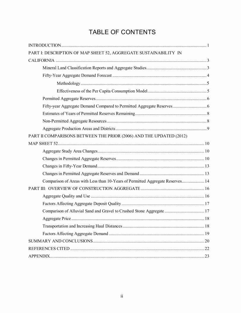
TABLE OF CONTENTS

INTRODUCTION ................................................................................................................................ 1

PART I: DESCRIPTION OF MAP SHEET 52, AGGREGATE SUSTAINABILITY IN

CALIFORNIA ..................................................................................................................................... 3

Mineral Land Classification Reports and Aggregate Studies ..................................................... 3

Fifty-Year Aggregate Demand Forecast ................................................................................... 4

Methodology ............................................................................................................... 5

Effectiveness of the Per Capita Consumption Model .................................................... 5

Permitted Aggregate Reserves.................................................................................................. 6

Fifty-year Aggregate Demand Compared to Permitted Aggregate Reserves .............................. 6 Estimates of Years of Permitted Reserves Remaining ............................................................... 8

Non-Permitted Aggregate Resources ........................................................................................ 8

Aggregate Production Areas and Districts ................................................................................ 9

PART II COMPARISONS BETWEEN THE PRIOR (2006) AND THE UPDATED (2012)

MAP SHEET 52 ................................................................................................................................. 10

Aggregate Study Area Changes .............................................................................................. 10

Changes in Permitted Aggregate Reserves.............................................................................. 10

Changes in Fifty-Year Demand .............................................................................................. 13

Changes in Permitted Aggregate Reserves and Demand ......................................................... 13

Comparison of Areas with Less than 10-Years of Permitted Aggregate Reserves .................... 14

PART III: OVERVIEW OF CONSTRUCTION AGGREGATE ........................................................ 16 Aggregate Quality and Use .................................................................................................... 16

Factors Affecting Aggregate Deposit Quality ......................................................................... 17

Comparison of Alluvial Sand and Gravel to Crushed Stone Aggregate ................................... 17

Aggregate Price ..................................................................................................................... 18

Transportation and Increasing Haul Distances ........................................................................ 18

Factors Affecting Aggregate Demand .................................................................................... 19

SUMMARY AND CONCLUSIONS .................................................................................................. 20

REFERENCES CITED ...................................................................................................................... 22

APPENDIX ........................................................................................................................................ 23

iii

TABLES

Table 1. Comparison of 50-year aggregate demand to permitted aggregate reserves for aggregate study areas as of January 1, 2011.................................................................... 7 Table 2. Comparison of permitted aggregate reserves between Map Sheet 52, 2006 and Map Sheet 52, 2012 ........................................................................................................ 11 Table 3. Comparison of 50-year demand between Map Sheet 52, 2006 and Map Sheet 52, 2012 ........................................................................................................ 12 Table 4. Percentage of permitted aggregate reserves as compared to 50-year demand for

Map Sheet 52, 2006 and Map Sheet 52, 2012 ............................................................... 15

iv

DEPARTMENT OF CONSERVATION CALIFORNIA GEOLOGICAL SURVEY

1

INTRODUCTION

Sand, gravel, and crushed stone are “construction materials.” These commodities, collectively referred to as aggregate, provide the bulk and strength to Portland Cement Concrete (PCC), Asphaltic Concrete (AC, commonly called “black top”), plaster, and stucco. Aggregate is also used as road base, subbase, railroad ballast, and fill. Aggregate normally provides from 80 to 100 percent of the material volume in the above uses.

The building and paving industries consume large quantities of aggregate and future demand for this commodity is expected to increase throughout California. Aggregate materials are essential to modern society, both to maintain the existing infrastructure and to provide for new construction. Therefore, aggregate materials are a resource of great importance to the economy of any area. Because aggregate is a low unit-value, high bulk weight commodity, it must be obtained from nearby sources to minimize economic and environmental costs associated with transportation. If nearby sources do not exist, then transportation costs can quickly exceed the value of the aggregate. Transporting aggregate from distant sources results in increased construction costs, fuel consumption, greenhouse gas emissions, air pollution, traffic congestion, and road maintenance. To give an idea of the scale of these impacts, from 1981 to 2010, California consumed an average of about 180 million tons of construction aggregate (all grades) per year. Moving in 25 ton truckloads that is over 7.2 million truck trips per year. With an average 25 mile haul (50 mile round trip) that amounts to more than 360 million truck miles traveled, almost 47 million gallons of diesel fuel used, and more than 520,000 tons of carbon dioxide emissions produced annually. If the haul distance is doubled to 50 miles (100 mile round trip) the numbers double to 721 million truck miles traveled, almost 94 million gallons of diesel fuel used, and over 1 million tons of carbon dioxide emissions produced. Land-use planners and decision makers in California are faced with balancing a wide variety of needs. Increasingly, as existing permitted aggregate supplies are depleted, local land-use decisions regarding aggregate resources can have regional impacts that go beyond local jurisdictional boundaries. These factors, universal need, increasing demand, the economic and environmental costs of transportation, and multiple land-use pressures make information about the availability and demand for aggregate valuable to land-use planners and decision makers charged with planning for a sustainable future for California’s citizens. California Geological Survey (CGS) Map Sheet 52, 1:1,100,000-scale, and this accompanying report provide general information about the current availability of, and future demand for, California’s permitted aggregate reserves. Map Sheet 52 was originally published in 2002 (Kohler 2002) and subsequently updated in 2006 (Kohler 2006). Map Sheet 52 (2012) is an update of the version published in 2006. Map Sheet 52 updates data from reports compiled by the CGS for 31 aggregate study areas throughout the state. These study areas cover about 30 percent of the state and provide aggregate for about 85 percent of California’s population. This report is divided into three parts: Part I provides data sources and methods used to derive the information presented; Part II compares the updated 2012 Map Sheet 52 to the prior (2006) map; and, Part III is an overview of construction

AGGREGATE SUSTAINABILITY IN CALIFORNIA MAP SHEET 52 (UPDATED 2012)

2

aggregate. All aggregate data and any reference to “aggregate” in this report and on the map pertain to “construction aggregate,” defined for this report as alluvial sand and gravel or crushed stone that meets standard specifications for use in PCC or AC unless otherwise noted. The estimates of permitted resources, aggregate demand, and years of permitted reserves remaining presented on Map Sheet 52 (2012) and in this report are based on conditions as of January 1, 2011 and do not reflect changes, such as production, mine closures, or new or expanded permits, that may have occurred since that time. Although the statewide and regional information presented on the map and in this report may be useful to decision-makers, it should not be used as a basis for local land-use decisions. The more detailed information on the location and estimated amounts of permitted and non-permitted resources, and future regional demands contained in each of the aggregate studies employed in the compilation of Map Sheet 52 should be used for local land-use and decision making purposes.


3

PART I: DESCRIPTION OF MAP SHEET 52, AGGREGATE SUSTAINABILITY IN CALIFORNIA

Map Sheet 52 is a statewide map showing a compilation of data about aggregate availability collected over a period of about 33 years and updated to January 1, 2011. The purpose of the map is to compare projected aggregate demand for the next 50 years with currently permitted aggregate reserves in 31 regions of the state. The map also shows the projected years of permitted reserves remaining and highlights regions where there is less than 10 years of permitted aggregate supply remaining. The following sections describe data sources and methodology that were used in the development of the map.

Mineral Land Classification Reports and Aggregate Studies Data regarding aggregate reserves and projected aggregate demand shown on Map Sheet 52 are updated from a series of mineral land classification reports published by CGS between 1981 and 2010 (see Appendix). They were prepared in response to California’s Surface Mining and Reclamation Act of 1975 (SMARA) that requires the State Geologist to classify land based on the known or inferred mineral resource potential of that land. SMARA, its regulations and guidelines, are described in Special Publication 51(Division of Mines and Geology, 2000). The Mineral Land Classification process identifies lands that contain economically significant mineral deposits. The primary goal of mineral land classification is to ensure that the mineral resource potential of lands is recognized and considered in land-use planning. The classification process includes an assessment of the quantity, quality, and extent of aggregate deposits in a study area. Mineral land classification reports may be specific to aggregate resources, may contain information about both aggregate and other mineral resources, or they may only contain information on minerals other than aggregate. Reports that focus on aggregate include aggregate resource classification and mapping, estimates of permitted and non-permitted aggregate resources, projected 50-year demand for aggregate resources, and an estimate of when the permitted reserves will be depleted. Map Sheet 52 is a statewide updated summary of 50-year demands and permitted resource calculations for all SMARA classification reports pertaining to construction aggregate. Mineral land classification studies for aggregate may use either a Production-Consumption (P-C) region or a County as the study area boundary. A P-C region is one or more aggregate production districts (a group of producing aggregate mines) and the market area they serve. P-C Regions sometimes cross county boundaries. Mineral land classification reports include information from one or more P-C regions, or from a county. For ease in discussion, the area covered by each P-C region or county aggregate study is referred to as an “aggregate study area”. These areas are shown at the lower left-hand corner of the map along with their respective report number and publication date. It should be noted that a report may include more than one aggregate study area. SMARA guidelines recommend that the State Geologist periodically review the mineral land classification in defined study regions to determine if new classifications are necessary. The projected 50-year forecast of aggregate demand in the region may also be revised. Fourteen


4

updated classification studies have been completed since the program began. Updated studies were completed by county:

• Los Angeles, • Orange, and • Ventura

or by P-C region

• South San Francisco Bay, • Monterey Bay, • Western San Diego County, • Fresno, Palm Springs, • Stockton-Lodi, • Claremont-Upland, • North San Francisco Bay (in progress) , • San Bernardino, • San Gabriel Valley, • Bakersfield, and • San Luis Obispo-Santa Barbara.

Since Los Angeles and Ventura counties had more than one P-C region, separate updated 50-year forecasts were made for each region. The Los Angeles County update (OFR 94-14) includes the San Fernando Valley, San Gabriel Valley, Saugus-Newhall, and the Palmdale P-C regions. The San Gabriel Valley P-C Region has since been updated separately. The Ventura County update (OFR 93-10) included the Western Ventura and the Simi Valley P-C regions. The index map of aggregate studies shown in the lower left hand corner of Map Sheet 52 shows the latest reports that cover an aggregate study area. Earlier reports covering the same areas or portions of areas are referenced in the Appendix with an asterisk (“*”).

Fifty-Year Aggregate Demand Forecast

The fifty-year aggregate demand forecast for each of the aggregate study areas is presented on Map Sheet 52 as a pie chart (See Fifty-Year Aggregate Demand Compared to Permitted Aggregate Reserves section), and also is presented in Table 1of this report. The demand information may be new, or updated from previously published mineral land classification reports. The demand forecast information depicted on Map Sheet 52 is for the period January 1, 2011 through December 2060. The aggregate study areas with the greatest projected future need for aggregate are South San Francisco Bay, Temescal Valley-Orange County, and Western San Diego County. Each is expected to require more than a billion tons of aggregate by the end of 2060. Other areas with projected high demands are San Gabriel Valley, and San Bernardino. Each of these areas is projected to need more than 800 million tons of aggregate in the next 50 years. Aggregate study areas having smaller demands generally are located in rural, less populated areas. The aggregate study areas of El Dorado County, Glenn County, Nevada County, Shasta County, Southern Tulare


5

County, Tehama County, and Western Merced County are all projected to require 100 million tons of aggregate or less over the next 50 years. Methodology Before selecting a method for predicting a 50-year aggregate demand, historical aggregate use was compared to such factors as housing starts, gross national product, population, and several other economic factors. It was found that the only factor showing a strong correlation to historical aggregate use was population change. Consequently, a per capita aggregate consumption forecast model is used for most of the aggregate study projections. This method of forecasting aggregate consumption benefits from its simplicity and the availability of population forecast data. The California’s Department of Finance (DOF) makes 50-year county population forecasts using U.S. census data. The steps used for forecasting California’s 50-year aggregate needs using the per capita consumption model are: 1) collecting yearly historical production and population data for a period of years ranging from the 1960s through 2010; 2) dividing yearly aggregate production by the population for that same year to determine annual historical per capita consumption; 3) projecting yearly population for a 50-year period from the beginning of 2011 through 2060; and, 4) multiplying each year of projected population by the average historical per capita consumption and adding the results for each year to obtain the 50-year aggregate demand. It should be noted that the years chosen to determine an average historical per capita consumption may differ depending upon historical aggregate use for that specific region. Effectiveness of the Per Capita Consumption Model

The assumption that each person will use a certain amount of aggregate every year is a simplification of actual usage patterns, but overall, an increase in the population leads to the use of more aggregate. Over long enough periods, perhaps 20 to 30 years or more, the random impacts of major public construction projects and economic recessions tend to be smoothed and consumption trends become similar to historic per capita consumption rates. Per capita consumption is a commonly used and accepted national, state, and regional measure for purposes of forecasting. The per capita consumption model has proved to be effective for projecting aggregate demand in major metropolitan areas. The Western San Diego and the San Gabriel Valley P-C regions are examples of how well the model works, having only a two percent (over 14 years) and an eight percent (over 29 years) difference, respectively, in actual versus projected aggregate demand (Miller, 1996, Kohler, 2010). However, the per capita model may not work well in county aggregate studies or in P-C regions that import or export a large percentage of aggregate resulting in a low correlation between P-C region production and population. In such areas, projections may be made based on historical production or multiple projections based on differing assumptions may be used to better characterize a range of future demand. For regions that export large amounts of aggregate to neighboring P-C regions, projections are based on an historical production model where 50-year aggregate demand is determined by extending a best-fit line of historical aggregate production data for a county or region. This model was used to project Yuba City-Marysville’s 50-year demand because the region exports about 70 percent its aggregate into neighboring areas such as Sacramento County and Placer County. In addition, the 50-year demand


6

for Glenn and Tehama counties, the Palmdale P-C region, and the Temescal Valley-Orange County area was also projected using this method.

Permitted Aggregate Reserves Approximately 4 billion tons of permitted aggregate reserves lie within the 31 aggregate study areas shown on Map Sheet 52. Permitted aggregate reserves are aggregate deposits that have been determined to be acceptable for commercial use, exist within properties owned or leased by aggregate producing companies, and have permits allowing mining of aggregate material. A “permit” is a legal authorization or approval by a lead agency, the absence of which would preclude mining operations. Although some permitted reserves face legal challenges, these reserves are included in this study pending resolution of those challenges. In California, mining permits usually are issued by local lead agencies (county or city governments). Map Sheet 52 shows permitted aggregate reserves as a percentage of the 50-year demand on each pie chart (See Fifty-Year Aggregate Demand Compared to Permitted Aggregate Reserves section). Beneath the study area name located next to its corresponding pie chart is the amount of permitted resource in tons along with the amount of 50-year demand. These figures are also given in Table 1. Tonnages are not given for Western Merced County and for the southern Tulare County to preserve proprietary company data. Permitted aggregate resource calculations shown on the map and in Table 1 initially were determined from information provided in reclamation plans, mining plans and use permits issued by the lead agencies. When information was inadequate to make reliable independent calculations, CGS staff used resource estimates provided by mine operators or owners. These data were checked against rough calculations made by CGS staff, and any major discrepancies were discussed with the mine operators or owners. Permitted resource calculations have been updated to account for production from 2006-2010 and are current as of the beginning of 2011.

Fifty-year Aggregate Demand Compared to Permitted Aggregate Reserves Fifty-year aggregate demand compared to the currently permitted aggregate reserves is represented by a pie chart for each of the 31 aggregate study areas shown on Map Sheet 52. Each pie chart is located in the approximate center of the aggregate study area it represents. There are four different sizes of charts, each size representing a 50-year demand range. The smallest pie chart represents 50-year demands ranging from 25 million to 200 million tons, while the largest chart represents demands of over 800 million tons. The amount of 50-year demand in tons is shown on the map along with the amount of permitted reserves beneath the study area name located next to its corresponding pie chart (permitted reserves, left / 50-year demand, right). The whole pie represents the total 50-year aggregate demand for a particular aggregate study area. The blue portion of the pie represents the permitted aggregate resource (shown as a percentage of the 50-year demand) while the purple-colored portion of the pie represents that portion of the 50-year demand that will not be met by the currently permitted reserves. For example, if the blue portion is 25 percent and the purple portion is 75 percent of a pie chart that represents a total demand of 400 million tons, the permitted reserves are 100 million tons, and the region will need an additional 300 million tons of aggregate to supply the area for the next 50 years. The pie representing the Placer County aggregate study area (north-central California) is completely colored blue showing permitted aggregate reserves are equal to or greater than the area’s 50-year aggregate demand.


7

1 Aggregate study areas follow either a Production-Consumption (P-C) region boundary or a county boundary. A P-C region includes one or more aggregate production districts and the market area that those districts serve. Aggregate resources are evaluated within the boundaries of the P-C Region. County studies evaluate all aggregate resources within the county boundary. 2 The County study has been divided into two areas, each having its own production and market area. A separate permitted resource calculation and 50-year forecast is made for each area. 3 Two P-C regions have been combined into one study area.

Table 1. Comparison of 50-year demand to permitted aggregate reserves for aggregate study areas as of January 1, 2011. (Study areas with ten or fewer years of permitted reserves are in bold type).

AGGREGATE STUDY AREA 1

50-Year Demand

(million tons)

Permitted Aggregate Reserves

(million tons)

Permitted Aggregate Reserves Compared to 50-Year Demand

(percent)

Projected

Years Remaining

Bakersfield P-C Region 438 143 33 21 to 30 Barstow-Victorville P-C Region 159 124 78 31 to 40 Claremont-Upland P-C Region 203 109 54 21 to 30 El Dorado County 76 18 24 11 to 20 Fresno P-C Region 435 46 11 10 or fewer Glenn County 59 33 56 21 to 30 Merced County2 Eastern Merced County Western Merced County

100 28

50

Proprietary

50

>50

21 to 30 31 to 40

Monterey Bay P-C Region 346 323 93 41 to 50 Nevada County 100 26 26 11 to 20 Palmdale P-C Region 577 152 26 11 to 20 Palm Springs P-C Region 295 152 52 21 to 30 Placer County 151 152 101 More than 50 North San Francisco Bay P-C Region 521 110 21 11 to 20 Sacramento County 670 42 6 10 or fewer Sacramento-Fairfield P-C Region 196 128 65 11 to 20 San Bernardino P-C Region 993 241 24 11 to 20 San Fernando Valley / Saugus-Newhall 3 476 77 16 10 or fewer

San Gabriel Valley P-C Region 809 322 40 11 to 20 San Luis Obispo-Santa Barbara P-C Region 240 75 31 11 to 20

Shasta County 93 52 56 21 to 30 South San Francisco Bay P-C Region 1,381 404 29 11 to 20 Stanislaus County 214 45 21 11 to 20 Stockton-Lodi P-C Region 436 232 53 31 to 40 Tehama County 62 32 52 21 to 30 Temescal Valley-Orange County 3 1,077 297 28 11 to 20 Tulare County2 Northern Tulare County Southern Tulare County

124 73

27

Proprietary

22

<50

11 to 20 21 to 30

Ventura County 3 298 96 32 11 to 20 Western San Diego County P-C Region 1,014 167 16 10 or fewer

Yuba City-Marysville P-C Region 403 392 97 41 to 50 Total 12,047 4,067 34


8

Except for Placer County, all of the aggregate study areas have less permitted aggregate reserves than they are projected to need for the next 50-years. Nineteen of the 31 aggregate study areas have less than half of the permitted reserves they are projected to need in the next 50 years. Estimates of Years of Permitted Reserves Remaining New to the 2012 update, the right hand column of Table 1 indicates the projected years of permitted reserves remaining for the various aggregate study areas. Calculations of depletion years are made by comparing the currently permitted reserves to the projected annual aggregate consumption in the study area on a year-by-year basis. This is not the same as dividing the total projected 50-year demand for aggregate by 50 because, as population increases, so does the projected annual consumption of aggregate for a study area. Data are presented as ranges; 10 or fewer, 11-20, 21-30, 31-40, 41-50, and more than 50 years. This information is included on the map beneath the study area name along with the permitted reserves and the projected 50-year demand. These estimates are based on conditions as of January 1, 2011 and do not reflect changes, such as new or expanded permits, that may have occurred since that time. Four of the 31 aggregate study areas – Western San Diego County, Sacramento County, Fresno County, and the San Fernando Valley-Saugus Newhall area – are projected to have less than 10 years of permitted aggregate reserves remaining as of January 1, 2011. They are highlighted by red halos around the pie charts on Map Sheet 52 and appear in bold type in Table 1. Thirteen of the 31 aggregate study areas have between 11 and 20 years of permitted aggregate reserves remaining. Several of these including the North and South San Francisco Bay study areas and the Palmdale, San Bernardino, San Gabriel Valley, Temescal Valley-Orange County and Ventura County study areas are in or adjacent to urban areas with high aggregate demands. Eight of the 31 aggregate study areas have between 21 and 30 years of permitted aggregate reserves remaining, three have more than 31 years remaining, two have more than 41 years and one (Placer County) has more than 50 years of permitted reserves remaining. These numbers are estimates and the actual lifespan of existing permitted reserves in a study area can be influenced by many factors. In periods of high economic growth, demand may increase, shortening the life of permitted reserves. Large projects, such as the construction or maintenance of major infrastructure, or rebuilding after a disaster such as an earthquake could also deplete permitted reserves more rapidly. Increased demand from neighboring regions with dwindling or depleted permitted reserves may also accelerate the depletion of permitted reserves in a study area. Conversely, a slow economy may reduce demand for a period of time, extending the life of permitted reserves, or new or expanded permits may be granted in a study area increasing the permitted reserves and the lifespan of permitted reserves in that area.

Non-Permitted Aggregate Resources Non-permitted aggregate resources are deposits that may meet specifications for construction aggregate, are recoverable with existing technology, have no land use overlying them that is incompatible with mining, and currently are not permitted for mining. While not shown on Map Sheet 52, non-permitted aggregate resources are identified and discussed in each of the mineral land classification reports used to compile the map (See Appendix). There are currently an


9

estimated 74 billion tons of non-permitted construction aggregate resources in the 31 aggregate study areas shown on the map. While this number seems large, it is unlikely that all of these resources will ever be mined because of social, environmental, or economic factors. The location of aggregate resources too close to urban or environmentally sensitive areas can limit or prevent their development. Resources may also be located too far from a potential market to be economic. In spite of such possible constraints, non-permitted aggregate resources are the most likely future sources of construction aggregate potentially available to meet California’s continuing demand. Factors used to calculate non-permitted resource amounts and to determine the aerial extent of these resources, are given in each of the aggregate classification reports listed in the Appendix.

Aggregate Production Areas and Districts Aggregate production areas are shown on the map by five different sizes of triangle. A triangle may represent one or more active aggregate mines. The relative size of each symbol corresponds to the amount of yearly production for each mine or group of mines. Yearly production was based on data from the Department of Conservation’s Office of Mine Reclamation (OMR) records for the calendar year 2010. The smallest triangle represents a production area that produces less than 0.5 million tons of aggregate in 2010. These triangles represent a single mine operation. About 90 percent of the production areas on the map fall into this category, and many are located in rural parts of the state. The largest triangle represents aggregate mining districts with production of more than 5 million tons in 2010. Only two aggregate production districts fall into this category – the Temescal Valley District in western Riverside County and the San Gabriel Valley District in Los Angeles County. It should be noted that, because of the economic slowdown from 2007 to 2010, the tonnages represented by the triangles on the 2012 map are different from those on the 2006 map.


10

PART II COMPARISONS BETWEEN THE PRIOR (2006) AND THE UPDATED (2012) MAP SHEET 52

The prior version of Map Sheet 52 was completed and published in 2006. Permitted aggregate resource data for that map were current as of January 1, 2006. Work conducted for that study took place during 2006. The latest aggregate production and location data available for the prior map were from 2005 records. The aggregate demand projections for the prior map were based on DOF county population projections from the 2000 U.S. census. Fifty-year aggregate demand from January 1, 2006 through the year 2055 was determined for 31 study areas. This updated Map Sheet 52 was completed and published in 2012. Permitted aggregate resource data for the updated map is current as of January 1, 2011. All work conducted for the updated study also took place during 2012. The latest aggregate production and location data available for the updated map are from 2010 records. The aggregate demand projections for the updated map were based on DOF county population projections from the 2010 U.S. census. Fifty-year aggregate demand from January 1, 2011 through the year 2060 was determined for 31 study areas. Changes have occurred in both aggregate supplies (permitted aggregate reserves) and in 50-year aggregate demand in the five years since the prior Map Sheet 52 update was completed. Changes in permitted aggregate reserves between the prior Map Sheet 52 (2006) and updated Map Sheet 52 (2012) are shown in Table 2. Table 3 compares the changes in 50-year demand between Map Sheet 52 (2006) and the updated 2012 map.

Aggregate Study Area Changes Six aggregate study areas on the original (2002) Map Sheet 52 were modified for the 2006 map, resulting in three fewer study areas. They included the Southern California P-C regions of Orange County, Temescal Valley, San Fernando Valley, Saugus-Newhall, Western Ventura County, and Simi Valley. These regions were combined into three regions when they began to run out of permitted reserves and became dependant on aggregate sources from neighboring regions. The importation of aggregate from neighboring regions typically results in longer haul distances, higher costs, and increased carbon dioxide emissions, air pollution, traffic congestion, and highway maintenance. The shift in supply area also results in more rapid depletion of permitted reserves in neighboring regions. No additional study areas have been combined in this update. It is likely that in some future update the San Fernando Valley-Saugus Newhall aggregate study area and the Palmdale study area may be combined as permitted reserves in the San Fernando Valley-Saugus Newhall aggregate study area are depleted.

Changes in Permitted Aggregate Reserves Twenty-four of the 31 study areas shown on the updated map experienced a decrease in permitted aggregate reserves since the 2006 map was completed (See Table 2). Included in these 24 areas are Western Merced County and Southern Tulare County. Permitted reserves for both of these county study areas cannot be shown because they are proprietary.


11

AGGREGATE STUDY AREA

Permitted Aggregate Reserves as of 1/1/06

(million tons) Map Sheet 52, 2006

Permitted Aggregate Reserves as of 1/1/11


Percent Difference

(%)

Bakersfield P-C Region 115 143 24 Barstow Victorville P-C Region 133 124 -7 Claremont-Upland P-C Region 147 109 -26 Eastern Merced County 53 50 -6 El Dorado County 19 18 -5 Fresno P-C Region 71 46 -35 Glenn County 17 33 94 Monterey Bay P-C Region 347 323 -7 Nevada County 31 26 -16 Northern Tulare County 12 27 125 North San Francisco Bay P-C Region 49 110 124 Palmdale P-C Region 181 152 -16 Palm Springs P-C Region 176 152 -14 Placer County 45 152 238 Sacramento County 67 42 -37 Sacramento-Fairfield P-C Region 164 128 -22 San Bernardino P-C Region 262 241 -8 San Fernando Valley-Saugus Newhall * 88 77 -13 San Gabriel Valley P-C Region 370 322 -13 San Luis Obispo-Santa Barbara P-C Region 77 75 -3 Shasta County 51 52 2 Southern Tulare County Proprietary Proprietary Proprietary South San Francisco Bay P-C Region 458 404 -12 Stanislaus County 51 45 -12 Stockton Lodi P-C Region 196 232 18 Tehama County 36 32 -11 Temescal Valley-Orange County* 355 297 -16 Ventura County (combined Western Ventura County and Simi Valley P-C Region)* 106 96 -9 Western Merced County Proprietary Proprietary Proprietary Western San Diego County P-C Region 198 167 -16 Yuba City-Marysville P-C Region 409 392 -4 Total 4,343 4,067 -6

* Two P-C Regions have been combined into one study area Table 2. Comparison of permitted aggregate reserves between Map Sheet 52, 2006 and Map Sheet 52, 2012.


12


50-Year Demand as of 1/1/06


50-Year Demand as of 1/1/11


Percent Difference

(%)

Bakersfield P-C Region 252 438 74 Barstow-Victorville P-C Region 179 159 -11 Claremont-Upland P-C Region 300 203 -32 Eastern Merced County 106 100 -6 El Dorado County 91 76 -16 Fresno P-C Region 629 435 -31 Glenn County 83 59 -29 Monterey Bay P-C Region 383 346 -10 Nevada County 122 100 -18 Northern Tulare County 117 124 6 North San Francisco Bay P-C Region 647 521 -19 Palmdale P-C Region 665 577 -13 Placer County 171 151 -12 Palm Springs P-C Region 295 295 0 Sacramento County 733 670 -9 Sacramento-Fairfield P-C Region 235 196 -17 San Bernardino P-C Region 1,074 993 -8 San Fernando Valley/Saugus Newhall * 457 476 4 San Gabriel Valley P-C Region 1,148 809 -30 San Luis Obispo-Santa Barbara P-C Region 243 240 -1 Shasta County 122 93 -24 Southern Tulare County 88 73 -17 Stanislaus County 344 214 -38 Stockton Lodi P-C Region 728 436 -40 South San Francisco Bay P-C Region 1,244 1381 11 Tehama County 72 62 -14 Temescal Valley-Orange County * 1,122 1,077 -4 Ventura County (combined Western Ventura County and Simi Valley P-C Regions) * 309 298 -4

Western Merced County 53 28 -47 Western San Diego County P-C Region 1,164 1014 -13 Yuba City-Marysville P-C Region 360 403 12 Total 13,536 12,047 -11

* Two P-C Regions have been combined into one study area Table 3. Comparison of 50-year demand between Map Sheet 52, 2006 and Map Sheet 52, 2012.


13

Seven of the study areas shown on the updated map had increases in permitted aggregate reserves. Most of these increases are because of newly permitted or expanded mining operations. An expansion may increase the footprint of the mine or increase permitted mining depth. Significant increases exceeding 50 percent occurred in the Placer County, Glenn County, Northern Tulare County, and the North San Francisco Bay aggregate study areas (See Table 2). Total permitted reserves for all 31 areas decreased from 4,343 million tons to 4,067 million tons – an apparent reduction of 276 million tons. Most of this reduction was because of aggregate consumption. Other potential reasons for reductions in permitted aggregate reserves include social and economic conditions leading to mine closures, regulatory changes, or natural variations in the quality of aggregate deposits. Actual production was greater but was offset in part by increases in permitted reserves in some study areas.

Changes in Fifty-Year Demand Of the 31 study areas shown on the updated Map Sheet 52 five had increases in 50-year demand, one remained constant, and 25 showed decreases in projected 50-year demand (See Table 3). The large number of study areas with decreasing 50-year demand is due in large part to the new population projections used in forecasting. The new county population projections (State of California Department of Finance, 2012) are based on the 2010 U.S. census and project lower growth rates for much of California compared to the projections used in the previous versions of this study. Newly updated per capita consumption numbers may also have contributed to changes in projected 50-year demand. The large increase (74 percent) in the 50-year demand for the Bakersfield study area is due to the use of newer population projections than were used in the original study and previous versions of this study.

Changes in Permitted Aggregate Reserves and Demand Table 4 shows the percentages of permitted reserves compared to the 50-year demand for the 2006 and updated 2012 Map Sheet 52. These percentages are represented on both maps as pie charts – the blue portion of the pie depicting percentage of the 50-year demand met with current permitted reserves. Increases occurred in 14 of the 29 study areas that can be compared and no change or decreases occurred in 15 study areas. The large increases in some of these study areas (Glenn County, North San Francisco Bay, Northern Tulare County, Placer County, Shasta County, and Stockton-Lodi) were because of new or expanded permits resulting in additional permitted aggregate reserves. Many of the small increases are not due to new or modified permits, but are a result of low production rates during the economic slowdown from 2007 to 2010 and the lower projected 50-year demand in many study areas based on updated population forecasts used in the 2012 update. Similarly those study areas with no change or small decreases may also have been influenced by these factors.


14

Comparison of Areas with Less than 10-Years of Permitted Aggregate Reserves The 2012 Map Sheet 52 shows four aggregate study areas with less than a 10-year supply of permitted aggregate reserves – Sacramento County, Fresno County, San Fernando Valley-Saugus Newhall, and the Western San Diego County P-C Regions. The map shows these areas with red halos around the pie charts. Compared to the 2006 version of the map, the San Fernando Valley-Saugus Newhall study area is a new addition to this group while the North San Francisco Bay and Northern Tulare County study areas have been removed.


15


Percentage of Permitted Aggregate

Reserves as Compared to 50-Year Demand as of 1/1/06 Map Sheet 52, 2006

Percentage of Permitted Aggregate

Reserves as Compared to 50-Year Demand as of 1/1/11 Map Sheet 52, 2012

Difference

Bakersfield P-C Region 46 33 -13 Barstow-Victorville P-C Region 74 78 4 Claremont-Upland P-C Region 49 54 5 Eastern Merced County 50 50 0 El Dorado County 21 24 3 Fresno P-C Region 11 11 0 Glenn County 21 56 35 Monterey Bay P-C Region 91 93 2 Nevada County 25 26 1 Northern Tulare County 10 22 12 North San Francisco Bay P-C Region 8 21 13 Palmdale P-C Region 27 26 -1 Palm Springs P-C Region 60 52 -8 Placer County 26 101 75 Sacramento County 9 6 -3 Sacramento-Fairfield P-C Region 70 65 -5 San Bernardino P-C Region 24 24 0 San Fernando Valley/Saugus Newhall * 19 16 -3 San Gabriel Valley P-C Region 32 40 8 San Luis Obispo-Santa Barbara P-C Region 32 31 -1 Shasta County 42 56 14 Southern Tulare County Proprietary Proprietary Stanislaus County 15 21 6 Stockton Lodi P-C Region 27 53 26 South San Francisco Bay P-C Region 37 29 -8 Tehama County 49 52 3 Temescal Valley-Orange County * 32 28 -4 Ventura County (combined Western Ventura County and Simi Valley P-C Regions) * 34 32 -2

Western Merced County Proprietary Proprietary Western San Diego County P-C Region 17 16 -1 Yuba City-Marysville P-C Region 100 97 -3

* Two P-C Regions have been combined into one study area

Table 4. Percentage of permitted aggregate reserves as compared to 50-year demand for Map Sheet 52, 2006 and Map Sheet 52, 2012.


16

PART III: OVERVIEW OF CONSTRUCTION AGGREGATE Construction aggregate was the leading non-fuel mineral commodity produced in California in 2010. Valued at $1.19 billion, aggregate made up about 41 percent of California’s $2.9 billion non-fuel mineral production in 2010.

Aggregate Quality and Use Aggregate normally makes up 80 to 100 percent of the material volume in PCC and AC and provides the bulk and strength to these materials. Rarely, even from the highest-grade deposits, is in-place aggregate physically or chemically suited for every type of aggregate use. Every potential deposit must be tested to determine how much of the material can meet specifications for a particular use, and what processing is required. Specifications for PCC, AC, and various other uses of aggregate have been established by several agencies, such as the U.S. Bureau of Reclamation, the U.S. Army Corps of Engineers, and the California Department of Transportation to ensure that aggregate is satisfactory for specific uses. These agencies and other major consumers test aggregate using standard test procedures of the American Society for Testing Materials (ASTM), the American Association of State Highway Officials, and other organizations. Most PCC and AC aggregate specifications have been established to ensure the manufacture of strong, durable structures capable of withstanding the physical and chemical effects of weathering and use. For example, specifications for PCC and concrete products prohibit or limit the use of rock materials containing mineral substances such as gypsum, pyrite, zeolite, opal, chalcedony, chert, siliceous shale, volcanic glass, and some high-silica volcanic rocks. Gypsum retards the setting time of portland cement; pyrite dissociates to yield sulfuric acid and an iron oxide stain; and other substances contain silica in a form that reacts with alkali substances in the cement, resulting in cracks and "pop-outs." Alkali reactions in PCC can be minimized by the addition of pozzolanic admixtures such as fly ash or naturally occurring pozzolanic materials. Pozzolans are siliceous or siliceous and aluminous material of natural or artificial origin that, in the presence of moisture, reacts with calcium hydroxide to form cementitious compounds. Specifications also call for precise particle-size distribution for the various uses of aggregate that is commonly classified into two general sizes: coarse and fine. Coarse aggregate is rock retained on a 3/8-inch or a #4 U.S. sieve. Fine aggregate passes a 3/8-inch sieve and is retained on a #200 U.S. sieve (a sieve with 200 weaves per inch). For some uses, such as asphalt paving, particle shape is specified. Aggregate material used with bituminous binder (asphalt) to form sealing coats on road surfaces shall consist of at least 90% by weight of crushed particles. Crushed stone is preferable to natural gravel in asphaltic concrete (AC) because asphalt adheres better to broken surfaces than to rounded surfaces and the interlocking of angular particles strengthens the AC and road base. The material specifications for PCC and AC aggregate are more restrictive than specifications for other applications such as Class II base, subbase, and fill. These restrictive specifications make deposits acceptable for use as PCC or AC aggregate, the scarcest and most valuable aggregate resources. Aggregate produced from such deposits can be, and commonly is, used in applications other than concrete. PCC- and AC-grade aggregate deposits are of major importance when planning for future availability of aggregate commodities because of their versatility, value, and relative scarcity.


17

Factors Affecting Aggregate Deposit Quality The major factors that affect the quality of construction aggregate are the rock type and the degree of weathering of the deposit. Rock type determines the hardness, durability, and potential chemical reactivity of the rock when mixed with cement to make concrete. In alluvial sand and gravel deposits, rock type is variable and reflects the rocks present in the drainage basin of the stream or river. In crushed stone deposits, rock type is typically less variable, although in some types of deposits, such as sandstones or volcanic rocks, there may be significant variability of rock type within a deposit. Rock type may also influence aggregate shape. For example, some metamorphic rocks such as slates tend to break into thin platy fragments that are unsuitable for many aggregate uses, while many volcanic and granitic rocks break into blocky fragments more suited to a wide variety of aggregate uses. Deposit type also affects aggregate shape. For example, in alluvial sand and gravel deposits, the natural abrasive action of the stream rounds the edges of rock particles, in contrast to the sharp edges of particles from crushed stone deposits. Weathering is the in-place physical or chemical decay of rock materials at or near the Earth’s surface. Weathering commonly decreases the physical strength of the rock and may make the material unsuitable for high strength and durability uses. Weathering may also alter the chemical composition of the aggregate, making it less suitable for some aggregate uses. If weathering is severe enough, the material may not be suitable for use as PCC or AC aggregate. Typically, the older a deposit is, the more likely it has been subjected to weathering. The severity of weathering commonly increases with increasing age of the deposit.

Comparison of Alluvial Sand and Gravel to Crushed Stone Aggregate The preferred use of one aggregate material over another in construction practices depends not only on specification standards, but also on economic considerations. Alluvial gravel is typically preferred to crushed stone for PCC aggregate because the rounded particles of alluvial sand and gravel result in a wet mix that is easier to work than a mix made of angular fragments. Also, crushed stone is less desirable in applications where the concrete is placed by pumping because sharp edges will increase wear and damage to the pumping equipment. The workability of a mix consisting of portland cement with crushed stone aggregate can be improved by adding more sand and water, but more cement must then be added to the mix to meet concrete durability standards. This results in a more expensive concrete mix and a higher cost to the consumer. In addition, aggregate from a crushed stone deposit is typically more expensive than that from an alluvial deposit due to the additional costs associated with the ripping, drilling and blasting necessary to remove material from most quarries and the additional crushing required to produce the various sizes of aggregate. Manufacturing sand by crushing is more costly than mining and processing naturally occurring sand. Although more care is required in pouring and placing a wet mix containing crushed stone, PCC made with this aggregate is as satisfactory as that made with alluvial sand and gravel of comparable rock quality. Owing to environmental concerns and regulatory constraints in many areas of the state, it is likely that extraction of sand and gravel resources from instream and floodplain areas will become less common in the future. If this trend continues, crushed stone may become increasingly important to the California market.


18

Aggregate Price The price of aggregate throughout California varies considerably depending on location, quality, and supply and demand. The highest quality aggregate, and typically most costly, is that which meets the California Department of Transportation’s specifications for use in Portland Cement Concrete (PCC). All prices discussed in this section are for PCC-grade aggregate at the plant site or FOB (freight on board). Transportation cost, which adds to the final cost of aggregate, is discussed in the next section. Regional variations make it difficult to estimate the average price of PCC-grade aggregate for the state. Over the last decade, prices have varied from $20 per ton or more in areas with depleting or depleted aggregate supplies and high demands to $7 to $8 per ton in areas with abundant aggregate supplies and low to moderate demands. In the last decade, the highest prices aggregate in the state have been in the San Diego area, where PCC-grade sand is in short supply, causing prices to range up to $20-$22 per ton and in parts of the San Francisco Bay area where sand has also been in short supply and prices have ranged from $15 to $19 per ton. In the Los Angeles metropolitan areas prices have been in the $13 to $16 per ton range with aggregate from the sparsely populated Palmdale area at about $10 per ton. Aggregate from Palmdale is also transported to Ventura County – a haul distance of about 60 miles, and into the San Fernando Valley-Saugus Newhall area. The cost of transportation in these cases adds significantly to the final cost of the aggregate. In the Central Valley, prices have ranged from $7 to $8 per ton in the Yuba City-Marysville area where aggregate supplies are abundant to $10 to $11 per ton in the Sacramento and Stockton-Lodi areas. In the Southern Valley, prices have been somewhat higher, about $12 per ton in the Bakersfield region and $14 to $18 per ton in the Fresno and northern Tulare areas.

Transportation and Increasing Haul Distances Transportation plays a major role in the cost of aggregate to the consumer. Aggregate is a low-unit-value, high-bulk-weight commodity, and it must be obtained from nearby sources to minimize both the dollar cost to the aggregate consumer and other environmental and economic costs associated with transportation. If nearby sources do not exist, then transportation costs may significantly increase the cost of the aggregate by the time it reaches the consumer. For straight hauls with minimal traffic, the price of aggregate increases about 15 cents per ton for every mile that it is hauled from the plant according to industry sources. Currently, transporting aggregate a distance of 30 miles will increase the FOB price by about $4.50 per ton. For example, to construct one mile of six-lane interstate highway requires about 113,500 tons of aggregate. Transporting this amount of aggregate 30 miles adds $510,000 to the base cost of the material at the mine. In major metropolitan areas, this rate is often greater because of heavy traffic that increases the haul time. Other factors that affect hauling rates include toll bridges and toll roads, road conditions, and routes in hilly or mountainous areas. Transportation cost is the principal constraint defining the market area for an aggregate mining operation.


19

Throughout California, aggregate haul distances have been gradually increasing as more local sources of aggregate diminish. Consequently, older P-C regions, most of which were established in the late 1970s have changed considerably since their boundaries were drawn. This is especially evident in Los Angeles, Orange, and Ventura counties where aggregate shortages have led to the merging of six P-C regions shown on the original (2002) map into three regions for the updated maps. Increased aggregate haul distances not only increase the cost of aggregate to the consumer, but also increase environmental and societal impacts such as increased fuel consumption, carbon dioxide emissions, air pollution, traffic congestion and road maintenance.

Factors Affecting Aggregate Demand Several factors may influence aggregate demand. In periods of high economic growth, demand may increase, depleting permitted reserves more rapidly than expected. Large projects, such as the construction or maintenance of major infrastructure, or rebuilding after a disaster such as an earthquake could also deplete permitted reserves more rapidly. Increased demand from neighboring regions with dwindling or depleted permitted reserves may also accelerate the depletion of permitted reserves in a study area. Conversely, a period of declining economy or of low economic growth, such as that during the recession of 2007 to 2009 and the subsequent slow economic recovery, can reduce demand for a period of time, extending the life of permitted reserves. In some cases, importation of aggregate from other areas may extend the life of a region’s permitted reserves.


20

SUMMARY AND CONCLUSIONS Aggregate is essential to the needs of modern society, providing material for the construction and maintenance of roadways, dams, canals, buildings and other parts of California’s infrastructure. Aggregate is also found in homes, schools, hospitals and shopping centers. In the 30-year period from 1981 to 2010, Californians consumed an average of more than 180 million tons of construction aggregate (all grades) per year or about 5.7 ton per person per year. Demand for aggregate is expected to increase as the state’s population continues to grow and infrastructure is maintained, improved, and expanded. Because aggregate is a low unit-value, high bulk weight commodity, it must be obtained from nearby sources to minimize the dollar cost to the aggregate consumer and other environmental and economic costs associated with transportation. For the last 33 years, under the Surface Mining and Reclamation Act, CGS has conducted on-going studies that identify and evaluate aggregate resources throughout the state. Map Sheet 52 (2012) is an updated summary of supply and demand data from these studies. The map presents a statewide overview of future aggregate needs and currently permitted reserves.

The following conclusions can be drawn from Map Sheet 52 (2012) and this accompanying report:

• In the next 50 years, the 31 study areas identified on Map sheet 52 (2012) will need

approximately 12 billion tons of aggregate.

• The 31 study areas currently have about 4 billion tons of permitted reserves, which is about one third of the total projected 50-year aggregate demand identified for these study areas. This is about 5.5 percent of the total aggregate resources located within the 31 study areas.

• Four of the aggregate study areas are projected to have 10 or fewer years of permitted aggregate reserves remaining as of January 2011 (pie charts highlighted with red borders).

• Thirteen of the 31 aggregate study areas have between 11 and 20 years of aggregate reserves remaining.

• Eight of the 31 aggregate study areas have between 21 and 30 years of aggregate reserves remaining.

• Three of the 31 aggregate study areas have between 31 and 40 years of aggregate reserves remaining.

• Two of the 31 aggregate study areas have between 41 and 50 years of aggregate reserves remaining

• One of the 31 aggregate study areas (Placer County) has more than 50 years of aggregate reserves remaining.


21

The information presented on Map Sheet 52 (2012) and in the referenced reports is provided to assist land use planners and decision makers in identifying those areas containing construction aggregate resources, and to quantify potential future demand for these resources in different regions of the state. This information is intended to help planners and decision makers balance the need for construction aggregate with the many other competing land use issues in their jurisdictions, and to provide for adequate supplies of construction aggregate to meet future needs.


22

REFERENCES CITED California Department of Transportation, 1992, Standard Specifications. Division of Mines and Geology, 2000, California surface mining and reclamation policies and procedures: Special Publication 51, third revision. Kohler, S.L., 2002, Aggregate Availability in California, California Geological Survey, Map Sheet 52, scale 1:1,100,000, 26p. Kohler, S.L., 2006, Aggregate Availability in California, California Geological Survey, Map Sheet 52 (Updated 2006), scale 1:1,100,000, 26p. Kohler, S.L., 2010, Update of mineral land classification for Portland cement concrete-grade aggregate in the San Gabriel Valley Production-Consumption Region, Los Angeles County, California. Miller, R.V., 1996, Update of minerals land classification: aggregate materials in the western San Diego County Production-Consumption Region. State of California, Department of Finance, Interim Population Projections for California and Its Counties 2010-2050, Sacramento, California, May 2012.


23

APPENDIX: MINERAL LAND CLASSIFICATION REPORTS BY THE CALIFORNIA GEOLOGICAL SURVEY (Special Reports and Open-File

Reports, with information on aggregate resources) SPECIAL REPORTS SR 132: Mineral Land Classification: Portland Cement Concrete-Grade Aggregate in the

Yuba City-Marysville Production-Consumption Region. By Habel, R.S., and Campion, L.F., 1986. *SR 143: Part I: Mineral Land Classification of the Greater Los Angeles Area: Description of

the Mineral Land Classification Project of the Greater Los Angeles Area. By Anderson T. P., Loyd, R.C., Clark, W.B., Miller, R.M., Corbaley, R., Kohler,

S.L., and Bushnell, M.M., 1979. *SR 143: Part II: Mineral Land Classification of the Greater Los Angeles Area: Classification

of Sand and Gravel Resource Areas, San Fernando Valley Production-Consumption Region.

By Anderson T.P., Loyd, R.C., Clark, W.B., Miller, R.M., Corbaley, R., Kohler, S.L., and Bushnell, M.M., 1979.

*SR 143: Part III: Mineral Land Classification of the Greater Los Angeles Area:

Classification of Sand and Gravel Resource Areas, Orange County-Temescal Valley Production-Consumption Region.

By Miller, R.V., and Corbaley, R., 1981. *SR 143: Part IV: Mineral Land Classification of the Greater Los Angeles Area:

Classification of Sand and Gravel Resource Areas, San Gabriel Valley Production-Consumption Region. By Kohler, S.L., 1982.

*SR 143: Part V: Mineral Land Classification of the Greater Los Angeles Area: Classification

of Sand and Gravel Resource Areas, Saugus-Newhall Production-Consumption Region and Palmdale Production-Consumption Region.

By Joseph, S.E, Miller, R.V., Tan, S.S., and Goodman, R.W., 1987. *SR 143: Part VI: Mineral Land Classification of the Greater Los Angeles Area:

Classification of Sand and Gravel Resource Areas, Claremont-Upland Production-Consumption Region. By Cole, J.W., 1987.

*SR 143: Part VII: Mineral Land Classification of the Greater Los Angeles Area:

Classification of Sand and Gravel Resource Areas, San Bernardino Production-Consumption Region. By Miller, R.V., 1987.


24

*SR 145: Part I: Mineral Land Classification of Ventura County: Description of the Mineral

Land Classification Project of Ventura County. By Anderson,T.P., Loyd, R.C., Kiessling, E.W., Kohler, S.L., and Miller, R.V., 1981.

*SR 145: Part II: Mineral Land Classification of Ventura County: Classification of the Sand,

Gravel, and Crushed Rock Resource Areas, Simi Production-Consumption Region. By Anderson,T.P., Loyd, R.C., Kiessling, E.W., Kohler, S.L., and Miller, R.V., 1981.

*SR 145: Part III: Mineral Land Classification of Ventura County: Classification of the Sand

and Gravel, and Crushed Rock Resource Areas, Western Ventura County Production-Consumption Region. By Anderson,T.P., Loyd, R.C., Kiessling, E.W., Kohler, S.L., and Miller, R. V., 1981.

*SR 146: Part I: Mineral Land Classification: Project Description: Mineral Land

Classification for Construction Aggregate in the San Francisco-Monterey Bay Area. By Stinson, M.C., Manson, M.W., and Plappert, J.J., 1987.

*SR 146: Part II: Mineral Land Classification: Aggregate Materials in the South San Francisco Bay Production-Consumption Region.

By Stinson, M.C., Manson, M.W., and Plappert, J.J., 1987. *SR 146: Part III: Mineral Land Classification: Aggregate Materials in the North San Francisco Bay Production-Consumption Region.

By Stinson, M.C., Manson, M.W., and Plappert, J.J., 1987. *SR 146: Part IV: Mineral Land Classification: Aggregate Materials in the Monterey Bay

Production-Consumption Region. By Stinson, M.C., Manson, M.W., and Plappert, J.J., 1987.

*SR 147: Mineral Land Classification: Aggregate Materials in the Bakersfield Production-

Consumption Region. By Cole, J.W., 1988.

*SR 153: Mineral Land Classification: Aggregate Materials in the Western San Diego County

Production-Consumption Region. By Kohler, S.L., and Miller, R.V., 1982.

SR 156: Mineral Land Classification: Portland Cement Concrete-Grade Aggregate in the Sacramento-Fairfield Production-Consumption Region. By Dupras, D.L., 1988.


25

*SR 158: Mineral Land Classification: Aggregate Materials in the Fresno Production-Consumption Region. By Cole, J.W., and Fuller, D.R., 1986.

*SR 159: Mineral Land Classification: Aggregate Materials in the Palm Springs Production-Consumption Region. By Miller, R.V., 1987.

*SR 160: Mineral Land Classification: Portland Cement Concrete-Grade Aggregate in the

Stockton-Lodi Production-Consumption Region. By Jensen, L.S., and Silva, M.A., 1989.

*SR 162: Mineral Land Classification: Portland Cement Concrete Aggregate and Active

Mines of All Other Mineral Commodities in the San Luis Obispo-Santa Barbara Production-Consumption Region. By Miller, R.V., Cole, J.W., and Clinkenbeard, J.P., 1989.

SR 164: Mineral Land Classification of Nevada County, California.

By Loyd, R.C., and Clinkenbeard, J.P., 1990.

SR 165: Mineral Land Classification of the Temescal Valley Area, Riverside County, California. By Miller, R.V., Shumway, D.O., and Hill, R.L., 1991.

SR 173: Mineral Land Classification of Stanislaus County, California.

By Higgins, C.T., and Dupras, D.L., 1993. SR 198: Update of Mineral Land Classification for Portland Cement Concrete-Grade

Aggregate in the Palm Springs Production-Consumption Region, Riverside County, California. Busch, L.L., 2007.

SR 199: Update of Mineral Land Classification for Portland Cement Concrete-Grade

Aggregate in the Stockton-Lodi Production-Consumption Region, San Joaquin and Stanislaus Counties, California. Smith, J.D. and Clinkenbeard J.P., 2012.

SR202 Update of Mineral Land Classification for Portland Cement Concrete-Grade

Aggregate in the Claremont-Upland Production-Consumption Region, Los Angeles and San Bernardino Counties, California. Miller, R.V. and Busch, L.L., 2007.

SR 205 Update of Mineral Land Classification of Aggregate Resources in the North San

Francisco Bay P-C Region: Sonoma, Napa, and Marin Counties and Southwestern Solano County, California. Miller, R.V. and Busch, L.L., 2012 (in progress)

SR206 Update of Mineral Land Classification for Portland Cement Concrete-Grade

Aggregate in the San Bernardino Production-Consumption Region, San Bernardino and Riverside Counties, California. Miller, R.V. and Busch, L.L., 2008.


26

SR 209 Update of Mineral Land Classification for Portland Cement Concrete-Grade Aggregate in the San Gabriel Valley Production-Consumption Region, Los Angeles County, California. Kohler, S.L., 2010.

SR 210 Update of Mineral Land Classification: Aggregate Materials in the Bakersfield

Production-Consumption Region, Kern County, California. Busch, L.L., 2009. SR 215 Update of Mineral Land Classification: Aggregate Materials in the San Luis

Obispo-Santa Barbara Production-Consumption Region, California. Busch, L.L. and Miller, R.V., 2011.

* These Mineral Land Classification reports have been updated and are not shown on the index

map (lower left-hand corner of Map Sheet 52). OPEN-FILE REPORTS OFR 92-06: Mineral Land Classification of Concrete Aggregate Resources in the Barstow-

Victorville Area. By Miller, R.V., 1993.

OFR 93-10: Update of Mineral Land Classification of Portland Cement Concrete Aggregate in Ventura, Los Angeles, and Orange Counties, California: Part I - Ventura County. By Miller, R.V., 1993.

OFR 94-14: Update of Mineral Land Classification of Portland Cement Concrete Aggregate in

Ventura, Los Angeles, and Orange Counties, California: Part II - Los Angeles County. By Miller, R.V., 1994.

OFR 94-15: Update of Mineral Land Classification of Portland Cement Concrete Aggregate in

Ventura, Los Angeles, and Orange Counties, California: Part III - Orange County. By Miller, R.V., 1995.

OFR 95-10: Mineral Land Classification of Placer County, California. By Loyd, R.C., 1995. OFR 96-03: Update of Mineral Land Classification: Aggregate Materials in the South San Francisco Bay Production-Consumption Region.

By Kohler-Antablin, S.L., 1996.

OFR 96-04: Update of Mineral Land Classification: Aggregate Materials in the Western San Diego County Production-Consumption Region. By Miller, R.V., 1996.

OFR 97-01: Mineral Land Classification of Concrete Aggregate Resources in the Tulare County

Production-Consumption Region, California. By Taylor, G.C., 1997. OFR 97-02: Mineral Land Classification of Concrete-Grade Aggregate Resources in Glenn

County, California. By Shumway, D.O., 1997.


27

OFR 97-03: Mineral Land Classification of Alluvial Sand and Gravel, Crushed Stone, Volcanic Cinders, Limestone, and Diatomite within Shasta County, California. By Dupras, D.L, 1997.

OFR 99-01: Update of Mineral Land Classification: Aggregate Materials in the Monterey Bay

Production-Consumption Region, California. By Kohler-Antablin, S.L., 1999.

OFR 99-02: Update of Mineral Land Classification: Aggregate Materials in the Fresno Production-Consumption Region, California. By Youngs, L.G. and Miller, R.V., 1999.

OFR 99-08: Mineral Land Classification of Merced County, California. By Clinkenbeard, J.P., 1999. OFR 99-09: Mineral Land Classification: Portland Cement Concrete-Grade Aggregate and Clay

Resources in Sacramento County, California. By Dupras, D.L., 1999. OFR 2000-03: Mineral Land Classification of El Dorado County, California.

By Busch L.L., 2001 OFR 2000-18: Mineral Land Classification of Concrete-Grade Aggregate Resources in Tehama

County, California. By Foster, B.D., 2001

Documents

AGGREGATE SUSTAINABILITY IN CALIFORNIA · PDF fileAGGREGATE SUSTAINABILITY IN CALIFORNIA . ... Moving in 25 ton ... the haul distance is doubled to 50 miles (100 mile round trip)