Aggregate Implications of Changing Sectoral Trends

WP 19-11R Andrew FoersterFederal Reserve Bank of San Francisco

Andreas Hornstein Federal Reserve Bank of Richmond

Pierre-Daniel SarteFederal Reserve Bank of Richmond

Mark WatsonPrinceton University and NBER

Aggregate Implications of Changing Sectoral Trends∗

Andrew T. Foerster Andreas Hornstein

Federal Reserve Bank of San Francisco Federal Reserve Bank of Richmond

Pierre-Daniel G. Sarte Mark W. Watson

Federal Reserve Bank of Richmond Princeton University and NBER

August 27, 2019

Abstract

We find disparate trend variation in TFP and labor growth across major U.S. production sectors

over the post-WWII period. When aggregated, these sector-specific trends imply secular declines in the

growth rate of aggregate labor and TFP. We embed this sectoral trend variation into a dynamic multi-

sector framework in which materials and capital used in each sector are produced by other sectors. The

presence of capital induces important network effects from production linkages that amplify the conse-

quences of changing sectoral trends on GDP growth. Thus, in some sectors, changes in TFP and labor

growth lead to changes in GDP growth that may be as large as three times these sectors’ share in the

economy. We find that trend GDP growth has declined by more than 2 percentage points since 1950, and

that this decline has been primarily shaped by sector-specific rather than aggregate factors. Sustained

contractions in growth specific to Construction, Nondurable Goods, and Professional and Business and

Services make up close to sixty percent of the estimated trend decrease in GDP growth. In addition, the

slow process of capital accumulation means that structural changes have endogenously persistent effects.

We estimate that trend GDP growth will continue to decline for the next 10 years absent persistent in-

creases in TFP and labor growth.

Keywords: trend growth, multi-sector model, production linkages

JEL Codes: C32, E23, O41

∗The views expressed herein are those of the authors and do not necessarily represent the views of the Federal ReserveBanks of San Francisco, Richmond, or the Federal Reserve System. We thank Jon Samuels of the Bureau of EconomicAnalysis for advice on the data, as well as Bill Dupor for a helpful discussion. We also thank John Fernald, Chad Jones,and participants at various university seminars and conferences for their comments and suggestions. Daniel Ober-Reynoldsand Eric LaRose provided outstanding research assistance. Andrew Foerster: andrew.foerster@sf.frb.org, Andreas Hornstein:andreas.hornstein@rich.frb.org, Pierre-Daniel Sarte: pierre.sarte@rich.frb.org, Mark Watson: mwatson@princeton.edu.

1

Working Paper No. 19-11R

1 Introduction

The U.S. economy is currently on track for the longest expansion on record in the aftermath of the Great

Recession. However, it has also become evident that output has been growing conspicuously slowly during

this expansion. Fernald et al. (2017) find that slow growth in total factor productivity (TFP) and a fall in

labor force participation are the main culprits behind this weak recovery. Importantly, the authors also find

that these adverse forces are mostly unrelated to the financial crisis associated with the Great Recession.

Cette et al. (2016) suggest that a slowdown in productivity growth that began prior to the Great Recession

reflects in part the fading gains from the Information Technology (IT) revolution.1 This view is consistent

with the long lags associated with the productivity effects of IT adoption found by Basu and Fernald (2001),

and the collapse of the dot-com boom in the early 2000s. Moreover, Decker et al. (2016) point to a decline

in business dynamism that began in the 1980s as an additional force underlying slowing economic activity.2

This paper highlights the steady decline in trend GDP growth over the post-war period, 1950 − 2016.

Building on Fernald et al. (2017), we explore the roles played by TFP and labor inputs in explaining this

secular decline, but we do so at a disaggregated sectoral level. We estimate an empirical model where, in

each industry, TFP growth and labor growth have unobserved persistent and transitory components, and

where each component can itself stem from either aggregate or idiosyncratic forces. The estimates reveal

that trends in TFP and labor growth have steadily decreased across a majority of U.S. sectors since 1950.

Interestingly, more than 2/3 of the secular decline in aggregate TFP growth results from the combination of

sector-specific disturbances, thus leaving only an ancillary role for the aggregate component. Therefore, if

technical progress in general purpose technologies has helped drive trends in sectoral TFP growth, this thrust

has not been shared widely enough across sectors to generate comovement in TFP growth. This finding aligns

with the observation in Decker et al. (2016) that over the last 30 years, manufacturing has gradually shifted

from producing “general purpose” technologies to producing “special purpose” technologies. Similarly to

TFP growth, trend labor growth has generally been dominated by sector-specific factors, especially after

1980 and the latter part of the post-war period. The decline in trend labor growth is especially large in

the Durable Goods sector, though even in that sector trend growth always remains positive. In general, we

find that secular changes in TFP and labor growth have been mostly driven by sector-specific rather than

common components.

We define the process of structural change in different sectors as concurrently determined by the observed

low frequency behavior of TFP and labor growth in those sectors. We then embed those changes into a

dynamic multi-sector framework in which materials and capital used by different sectors in the economy are

1From a measurement standpoint, Byrne et al. (2016) also argue that the slowdown in TFP growth that preceded the lastrecession is not likely the result of mismeasurement of IT related goods and services. Aghion et al. (2017) find that the processof creative destruction does lead growth to be understated when inflation is imputed from surviving products. However, thismissing growth did not accelerate much after 2005, and was roughly constant before then.

2Fernald and Jones (2014) more generally make the case that diminishing marginal returns to the discovery of ideas ultimatelycurbs economic expansion. Gordon (2014) points to additional headwinds that have contributed to a general slowdown in growth,while Gordon and Sayed (2019) argue that a similar slowdown has taken place in the ten largest European economies.

2

produced by other sectors. We use balanced-growth accounting to determine the aggregate effects of sectoral

changes in trend rates of growth in labor and TFP. This paper, therefore, falls partially within the literature

on equilibrium multi-sector models first developed by Long and Plosser (1983), and later Horvath (1998,

2000), and Dupor (1999). Since then, a large body of work including Gabaix (2011), Foerster et al. (2011),

Acemoglu et al. (2012), di Giovanni et al. (2014), Atalay (2017), Baqaee and Farhi (2017b), Miranda-Pinto

(2019), and others have worked out important features of those models for generating aggregate fluctuations

from idiosyncratic shocks.3 In contrast to this literature, the focus herein centers on the implications of

production linkages for secular dynamics and the determination of both sectoral and aggregate trend growth

rates.4 While recent work has suggested a somewhat muted role for aggregate shocks in explaining cyclical

variations in GDP growth, we now find that sector-specific disturbances also explain most of the trend

variations in U.S. GDP growth.

Our paper returns to the original multi-sector model of Long and Plosser (1983) and maintains the origi-

nal assumptions of competitive input and product markets as well as constant-returns-to-scale technologies.

However, we explicitly allow different industries to produce investment goods for other industries. Unlike

Horvath (1998) or Dupor (1999), capital is not constrained to be sector-specific and is allowed to depreciate

only partially within the period. We assume unit elastic preferences and technologies that allow us to derive

analytical expressions for the model’s sectoral and aggregate balanced growth paths. These expressions

highlight how changes in trend TFP or labor growth in different sectors affect value added growth in every

other sector and, therefore, GDP growth. The implied elasticities reflect induced changes in capital trend

growth rates across sectors. Thus, our analysis in part extends Greenwood et al. (1997) to a multi-sector

environment.5

The fact that changes in TFP or labor growth in a sector affect value added growth in every other

sector hinges critically on the presence of capital. This feature of the environment leads to quantitatively

important multiplier effects from sectoral linkages to GDP growth. The size of this multiplier for a sector

depends on its importance as a supplier of capital or materials to other sectors. The density of production

linkages more generally determines the degree to which the sectoral network propagates structural changes

in a sector to the rest of the economy. The U.S. Capital Flow tables produced by the Bureau of Economic

Analysis (BEA) indicate that the Construction and Durable Goods sectors produce roughly 80 percent of

the capital used in almost every industry. The strength of these linkages results in GDP growth multipliers

for those sectors that are almost 3 times their share in the economy. Professional and Business Services and

3An additional dimension of this work explores the implications of frictions for aggregate fluctuations in these models,including Bigio and La‘O (2016), Baqaee (2018), Grassi (2018), and Baqaee and Farhi (2017a). Other recent work has alsoinvestigated the implications of production linkages for higher order moments, for instance Acemoglu et al. (2017), and Atalayet al. (2018)

4Ngai and Pissarides (2007) provide a seminal study of balanced growth in a multi-sector environment. They considerboth multiple intermediates and multiple capital-producing sectors but not at the same time. More importantly, the analysisabstracts from pairwise linkages in both intermediates and capital-producing sectors that play a key role in this paper.

5Basu et al. (2013) also construct a multi-sector extension of the Greenwood et al. (1997) environment, but they work withan aggregate capital stock and an aggregate labor endowment with each factor being perfectly mobile across sectors. In contrastto this paper, the authors study short-run responses to TFP shocks.

3

Wholesale Trade are also associated with relatively large GDP growth multipliers because of their central

role as suppliers of materials. We find that changing sectoral trends in the last 6 decades, translated through

the economy’s production network, have on net lowered trend GDP growth by roughly 2.2 percentage points.

Construction more than any other sector stands out by a considerable margin for its contribution to the

trend decline in GDP growth since 1950, accounting for close to 1/3 of this decline. Structural changes in

Professional and Business Services and Nondurable Goods together account for another 25 percent.

This paper is organized as follows. Section 2 gives an overview of the behavior of trend GDP growth over

the past 60 years. Section 3 provides an empirical description of TFP and labor growth by industry that

allows for persistent and transitory components, where each component itself may be driven by idiosyncratic

or aggregate forces. Section 4 develops the implications of these structural changes at the sector level in the

context of a dynamic multi-sector model with production linkages in materials and investment. This model

serves as the balanced growth accounting framework that we use to determine the aggregate implications of

changes in the sectoral trend growth rates of labor and TFP. Section 5 presents our quantitative findings.

Section 6 concludes and discusses possible directions for future research.

2 The Long-Run Decline in U.S. GDP Growth

Figure 1 shows the behavior of U.S. GDP growth over the post-WWII period. Here, GDP is measured

annually as the share-weighted value added from 16 sectors comprising the private U.S. economy; details

are provided in the next section.

Panel A shows aggregate private-sector growth rates computed using time-varying shares (i.e., chain-

weighting) and using average shares (fixed-weights), with virtually no difference between the two calculations.

Panel A shows large variation in GDP growth rates – the standard deviation is 2.5 percent over the period

1950− 2016 – but much of this variation is relatively short-lived and is associated with business cycles and

other relatively transitory phenomena. Our interest here is in longer-run variation.

Panel B, therefore, plots centered 15−year moving averages of the annual growth rates. Here too there

is variability. In the 1950s and early 1960s average annual growth exceeded 4 percent. This fell to 3 percent

in the 1970s, rebounded to nearly 4 percent in the 1990s, but plummeted to less than 2 percent in the 2000s

(See Table 1).

Panels C and D refine these calculations by eliminating the cyclical variation using an Okun’s law

regression in GDP growth rates as in Fernald et al. (2017).6 Thus, panel C plots the residuals from a

regression of GDP growth rates onto a short distributed lead and lag of changes in the unemployment rate

(∆ut+1,∆ut,∆ut−1). This cyclical adjustment eliminates much of the cyclical variability evident in panel

A. In addition, the 15−year moving average in Panel D now produces a more focused picture of the trend

variation in the growth rate of private GDP.

6Compared to other measures of cyclical slack or resource utilization, Fernald et al. (2017) point out that the civilianunemployment rate has two key advantages. First, it has been measured using essentially the same survey instrument since1948. Second, changes in the unemployment rate have nearly a mean of zero over long periods.

4

Figure 1: US GDP Growth Rates 1950-2016(Percentage points at an annual rate)

1950 1960 1970 1980 1990 2000 2010 2020-5

0

5

10A: GDP Growth

Constant Mean WeightsTime-Varying Weights

1950 1960 1970 1980 1990 2000 2010 20200

1

2

3

4

5B: GDP Growth, 15-Year Centered Moving Average

1950 1960 1970 1980 1990 2000 2010 2020-1

0

1

2

3

4

5

6C: Cyclically Adjusted GDP Growth

1950 1960 1970 1980 1990 2000 2010 20200

1

2

3

4

5

D: Cyclically-Adjusted GDP Growth,15-Year Centered Moving Average

Notes: Growth rates are share-weighted value added from 16 sectors making up the private U.S. economy. Cyclicaladjustment uses a regression on leads and lags of the first-difference in the unemployment rate.

The numbers reported in Table 1 frame the key question of this paper: why did the average growth rate

of GDP fall from 4 percent per year in the 1950s to just over 3 percent in the 1980s and 1990s, and then

further decline precipitously in the 2000s? We look to inputs – specifically TFP and labor at the sectoral

level – for the answer. That is, interpreting the data as variations around a balanced growth path, changes

in GDP growth are primarily determined by changes in the growth rates of those two inputs. However,

5

Table 1: 15-Year Averages of GDP Growth Rates

Dates Growth rates Cyclically-adjustedgrowth rates

1950− 2016 3.3 3.2

1950− 1965 4.3 4.11966− 1982 3.1 3.71983− 1999 3.9 3.32000− 2016 1.8 1.9

Notes: The values shown are averages of the series plotted inFigure 1, panels (A) and (C), over the periods shown.

as the analysis in Section 4 makes clear, not all sectoral inputs are created equal. Some sectors have a

large value-added share in GDP and also provide a large share of materials or capital to other sectors. Put

another way, input variation across sectors is a particularly important driver of low frequency movements

in aggregate GDP growth.

Before investigating these input-output interactions, we begin by describing the sectoral data, both how

these data are measured and how sectoral value-added as well as labor and TFP inputs have evolved over

the post-WWII period.

3 An Empirical Description of Trend Growth in TFP and Labor

We begin by estimating an empirical model of TFP and labor growth for different sectors of the U.S.

economy. As a benchmark, our paper applies the insights of Hulten (1978) on the interpretation of aggregate

productivity (TFP) changes as a weighted average of sector-specific value-added TFP changes. In particular,

under constant-returns-to-scale and perfect competition in product and input markets, the sectors’ weights

are the ratios of their valued added to GDP. 7 We calculate standard TFP growth rates at the sectoral level

following Jorgenson et al. (2017) among others, and estimate permanent and transitory components in these

growth rates.

3.1 Data

Sectoral TFP growth rates are calculated using the KLEMS dataset constructed by Jorgenson and his

collaborators, as well as its recently updated version in the form of the BEA’s Integrated Industry-Level

Production Accounts (ILPA). These datasets are attractive for our purposes because they provide a unified

7In the absence of constant-returns-to-scale or perfect competition, Basu and Fernald (1997, 2001) and Baqaee and Farhi(2018) show that aggregate TFP changes also incorporate reallocation effects. These effects reflect the movement of inputsbetween low and high returns to scale sectors stemming from changes in relative sectoral TFP.

6

approach to the construction of gross output, the primary inputs capital and labor, as well as intermediate

inputs (‘materials’) for a large number of industries. The KLEMS data are based on U.S. National Income

and Product Accounts (NIPA) and consistently integrate industry data with Input-Output tables and Fixed

Asset tables. The KLEMS dataset contains quantity and price indices for inputs and outputs across 65

industries. The growth rate of any one industry’s aggregate is defined as a Divisia index given by the

value-share weighted average of its disaggregated component growth rates. Labor input is differentiated

by gender, age, education, and labor status. Labor input growth is then defined as a weighted average of

growth in annual hours worked across all labor types using labor compensation shares of each type as weights.

Similarly, intermediate input growth reflects a weighted average of the growth rate of all intermediate inputs

averaged using payments to those inputs as weights. Finally, capital input growth reflects a weighted average

of growth rates across 53 capital types using payments to each type of capital as weights. Capital payments

are based on implicit rental rates consistent with a user-cost-of-capital approach. Total payments to capital

are the residuals after deducting payments to labor and intermediate inputs from the value of production.

Put another way, there are no economic profits.

An industry’s TFP growth rate is defined in terms of its Solow residual, specifically output growth less

the revenue-share weighted average of input growth rates. This calculation is consistent with the canonical

theoretical framework we adopt in Section 4 where all markets operate under perfect competition and

production is constant-returns-to-scale. For earlier versions of Jorgenson’s KLEMS data up to 1990, Basu

and Fernald (1997, 2001) compute total payments to capital as the sum of rental rates implied by the

user-cost-of-capital and find small industry profits on average that amount at most to three percent of gross

output. In the presence of close to zero profits, elasticities to scale and markups are equivalent. Basu and

Fernald (2001) estimate returns-to-scale across industries and find few significant deviations from constant

returns or, alternatively, little evidence of markups. More recently, an active debate has emerged on the

extent to which the competitive environment has changed in the U.S. over the last two decades. On the

one hand, Barkai (2017), also applying the user-cost-of-capital framework but using post 1990 data, finds

substantial profit shares over that period. Moreover, De Loecker and Eeckhout (2017), estimating industry

production functions from corporate balance sheets, present evidence of rising markups and returns to

scale since the 1980s. On the other hand, Karabarbounis and Neiman (2018) argue that the user-cost-

of-capital framework, to the extent that it implies high profit shares starting in the 1990s, also implies

unreasonably high profit shares in the 1950s. In addition, Traina (2018) argues that the evidence on rising

markups from corporate balance sheets depends crucially on the measurement of variable costs and weights

in aggregation.8 In this paper, we maintain the assumptions of competitive markets and constant-returns-

to-scale as a benchmark from which to study the aggregate implications of sectoral changes in labor and

TFP inputs.

8Similarly, Rossi-Hansberg et al. (2018) show while sales concentration has unambiguously risen at the national level sincethe 1980s, concentration has steadily declined at the Core-Based Statistical Area, county, and ZIP code levels over the sameperiod. While these facts can seem conflicting, the authors present evidence that large firms have become bigger through theopening of more establishments or stores in new local markets, but this process has lowered concentration in those markets.

7

Our calculations rely on the 2017 version of the Jorgenson KLEMS dataset which covers the period

1946− 2014, and the ILPA KLEMS dataset which covers the period 1987− 2016.9 For ease of presentation,

and in order to consider the role of structural change in individual sectors separately, we carry out the

empirical analysis using private industries at the two-digit level. In particular, we aggregate the 65 industries

included in the two KLEMS datasets into 16 two-digit private industries following the procedure in Hulten

(1978).10 Another advantage of the aggregation into two-digit industries is that any differences between

the two KLEMS datasets are attenuated and we feel comfortable splicing the levels of the two datasets in

1987.11 That is, we use the growth rates calculated using the Jorgenson KLEMS data before 1987 and using

ILPA data after that date.

Finally, we note that the KLEMS data rely on U.S. NIPA measures for fixed assets. Specifically, these

measures are based in part on estimates of capital goods prices. To the degree that these prices perennially

understate quality growth in capital goods, then KLEMS data understate productivity improvements in the

investment goods sector.12 If capital accumulation is an important driver of growth, our results would then

provide a lower bound for the growth contributions of the capital goods producing sectors.

Table 2 lists the 16 sectors we consider. For each sector, the table shows average cyclically adjusted

growth rates of value added, labor, and TFP over 1950 − 2016, and it also shows their average shares in

aggregate value added and labor input. The aggregate growth rates in the bottom row are the value-weighted

averages of the sectoral growth rates with average value added and labor shares used as fixed weights.

Clearly sectors grow at different rates and this disparity is hidden in studies that only consider aggregates.

Average real value added growth rates range from 1.1 percent in Mining to 4.7 percent in Wholesale Trade,

bracketing the aggregate value added growth rate of 3.2 percent. With the exception of the Durable Goods

sector, most sectors with growth rates that exceed the aggregate growth rate provide services. Similarly,

labor input growth rates range from a negative 1.4 percent in Agriculture to 3.3 percent in Professional

and Business Services, bracketing the average aggregate growth rate of 1.5 percent. Again, most sectors

with labor input growth rates that exceed the aggregate growth rate provide services. Finally, TFP growth

rates range from -0.9 percent in FIRE (ex-Housing) to 3.2 percent in Agriculture, bracketing the average

aggregate TFP growth rate of 0.6 percent. Sectoral TFP growth rates are less aligned with either value

added or labor input growth rates. There are three sectors with notable TFP declines, namely Utilities,

Other Services, and Construction, as well as a number of sectors with stagnant TFP levels. Negative TFP

9The Jorgenson dataset is downloaded from http://www.worldklems.net/data.htm and the ILPA is downloaded fromhttps://www.bea.gov/data/special-topics/integrated-industry-level-production-account-klems. A detailed descrip-tion of the Jorgenson data can be found in Jorgenson et al. (2014), as well as Jorgenson et al. (2017), and the BEA dataset isdescribed in Fleck et al. (2014).

10 The procedure is described in detail in the online-only Technical Appendix and Supplementary Material to this paper,Foerster et al. (2019).

11 While the ILPA builds on the Jorgenson KLEMS data, the two datasets are not exactly identical for the time period inwhich they overlap. Since both datasets are constructed to be consistent with the BEA’s input-output tables, they mostly agreeon industry details and both cover the same 65 private industries. Nevertheless, there remain differences but these are reflectedmostly in the levels of variables and not their growth rates.

12 See Gordon (1990) or Cummins and Violante (2002).

8

Table 2: 16 Sector Decomposition of the U.S. Private Economy(1950-2016)

Sectors Average growth rate Average share

Cyclically adjusted data (Percentage points)

(Percentage points at an

annual rate)

ValueAdded

Labor TFP ValueAdded

Labor

1 Agriculture 2.63 -1.42 3.16 2.70 3.25

2 Mining 1.06 0.27 -0.06 2.15 1.66

3 Utilities 1.87 0.98 -0.74 2.42 1.05

4 Construction 1.67 1.60 -0.10 5.04 7.64

5 Durable goods 3.36 0.42 1.88 13.48 15.59

6 Nondurable goods 2.29 0.07 0.79 9.31 8.84

7 Wholesale trade 4.65 1.68 1.13 6.92 6.50

8 Retail trade 3.16 1.08 1.07 8.44 9.86

9 Trans. & Ware. 2.43 0.85 1.35 4.19 4.91

10 Information 4.58 1.30 0.86 4.90 3.68

11 FIRE (x-Housing) 3.93 2.78 -0.90 10.03 7.41

12 PBS 4.36 3.26 0.30 8.59 10.88

13 Educ. & Health 3.32 2.75 0.04 6.01 9.28

14 Arts, Ent., & Food svc. 2.44 2.00 0.22 3.70 4.67

15 Other services (x-Gov) 2.02 2.38 -0.60 2.98 4.50

16 Housing 3.51 1.68 0.43 9.15 0.25

Aggregate 3.24 1.49 0.62 100 100

Notes: The values shown are average annual growth rates for the 16 sectors. The row labelled“Aggregate” is the share-weighted average of the 16 sectors.

growth rates are a counter-intuitive but well known feature of disaggregated industry data. To the degree

that they occur in service industries, they are in part attributed to measurement issues with respect to

output.

To a first approximation, the contributions of the different sectors to aggregate outcomes are given

by the nominal value added and labor input shares in the last two columns. Two notable contributors

to value added and TFP are Durable Goods and FIRE excluding Housing. The two largest contributors

to labor payments are Durable Goods and Professional and Business Services. Over time, the shares of

goods-producing sectors has declined while the shares of services-producing sectors has increased. However,

9

despite these changes, aggregating sectoral outputs and inputs using constant mean shares, as opposed to

time-varying shares, has little effect on the measurement of aggregate outputs and inputs (Figure 1A).

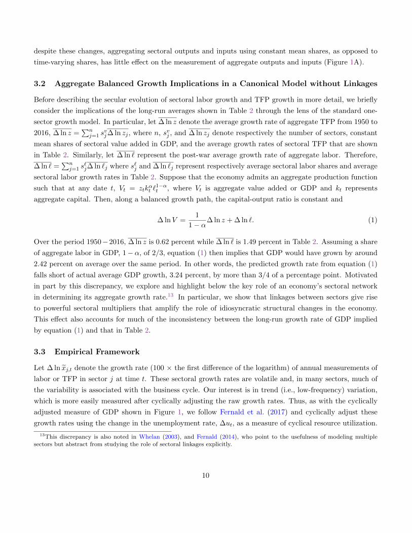
3.2 Aggregate Balanced Growth Implications in a Canonical Model without Linkages

Before describing the secular evolution of sectoral labor growth and TFP growth in more detail, we briefly

consider the implications of the long-run averages shown in Table 2 through the lens of the standard one-

sector growth model. In particular, let ∆ ln z denote the average growth rate of aggregate TFP from 1950 to

2016, ∆ ln z =∑n

j=1 svj∆ ln zj , where n, svj , and ∆ ln zj denote respectively the number of sectors, constant

mean shares of sectoral value added in GDP, and the average growth rates of sectoral TFP that are shown

in Table 2. Similarly, let ∆ ln ` represent the post-war average growth rate of aggregate labor. Therefore,

∆ ln ` =∑n

j=1 s`j∆ ln `j where s`j and ∆ ln `j represent respectively average sectoral labor shares and average

sectoral labor growth rates in Table 2. Suppose that the economy admits an aggregate production function

such that at any date t, Vt = ztkαt `

1−αt , where Vt is aggregate value added or GDP and kt represents

aggregate capital. Then, along a balanced growth path, the capital-output ratio is constant and

∆ lnV =1

1− α∆ ln z + ∆ ln `. (1)

Over the period 1950−2016, ∆ ln z is 0.62 percent while ∆ ln ` is 1.49 percent in Table 2. Assuming a share

of aggregate labor in GDP, 1−α, of 2/3, equation (1) then implies that GDP would have grown by around

2.42 percent on average over the same period. In other words, the predicted growth rate from equation (1)

falls short of actual average GDP growth, 3.24 percent, by more than 3/4 of a percentage point. Motivated

in part by this discrepancy, we explore and highlight below the key role of an economy’s sectoral network

in determining its aggregate growth rate.13 In particular, we show that linkages between sectors give rise

to powerful sectoral multipliers that amplify the role of idiosyncratic structural changes in the economy.

This effect also accounts for much of the inconsistency between the long-run growth rate of GDP implied

by equation (1) and that in Table 2.

3.3 Empirical Framework

Let ∆ ln xj,t denote the growth rate (100 × the first difference of the logarithm) of annual measurements of

labor or TFP in sector j at time t. These sectoral growth rates are volatile and, in many sectors, much of

the variability is associated with the business cycle. Our interest is in trend (i.e., low-frequency) variation,

which is more easily measured after cyclically adjusting the raw growth rates. Thus, as with the cyclically

adjusted measure of GDP shown in Figure 1, we follow Fernald et al. (2017) and cyclically adjust these

growth rates using the change in the unemployment rate, ∆ut, as a measure of cyclical resource utilization.

13This discrepancy is also noted in Whelan (2003), and Fernald (2014), who point to the usefulness of modeling multiplesectors but abstract from studying the role of sectoral linkages explicitly.

10

That is, we estimate

∆ ln xj,t = µj + βj(L)∆ut + ej,t, (2)

where βj(L) = βj,1L + βj,0 + βj,−1L−1 and the leads and lags of ∆ut captures much of the business-cycle

variability in the the data. Throughout the remainder of the paper, we use ∆ lnxj,t = ∆ ln xj,t− βj(L)∆ut,

where βj(L) denotes the OLS estimator, and where xj,t represents the implied cyclically adjusted value of

sector TFP (denoted zj,t) or labor input (denoted `j,t) growth rates.14

Figures 2 and 3 plot centered 15−year moving averages of the cyclically adjusted growth rates of labor

and TFP. These are shown as the thick blue lines in the figures (ignore the thin dotted red line for now).

The disparity in experiences across different sectors stands out. In particular, the moving averages show

large sector-specific variation through time. For example, labor input was contracting at nearly 4 percent

per year in agriculture in the 1950s, but stabilized near the end of the sample. In contrast, labor input in

the Durables and Nondurable goods sectors was increasing in the 1950s, but has been contracting since the

mid-1980s. At the same time, the rate of growth of labor in several service sectors are shown to exhibit

large ups and downs over the sample. Looking at TFP, there are important differences across sectors as

well. In Sections 4 and 5, we quantify the aggregate implications of these sectoral variations in labor and

TFP inputs.

In the economic model presented in Section 4, we treat zj,t and `j,t as exogenous processes and study

the implied values of output and value-added that arise from realizations of these processes. We do so in a

dynamic model that features input-output and capital flow linkages between the sectors. This multi-sector

accounting exercise requires joint stochastic processes for the sectoral values of zj,t and `j,t. For this purpose,

we use a reduced-form statistical model that captures the salient cross-sectional and dynamic correlations

in the data.

Cross-correlations and autocorrelations summarized in the online Technical Appendix suggest a reduced-

form model with three features. First, the sectoral growth rates of labor (∆`j,t) are somewhat correlated

across sectors; there is also (weak) cross-sector long-run correlation in the sectoral TFP growth rates (∆zj,t).

Second, there is little evidence of long-run correlation between (∆`j,t) and (∆zj,t) across or within sectors.15

Finally, ∆ ln `j,t and ∆ ln zj,t exhibit substantial year-to-year variation around slowly varying levels.

These features lead us to consider independent stochastic processes for ∆ ln `j,t and ∆ ln zj,t, where

the processes have a structure that includes factors common to all sectors together with sector-specific

factors, and where these factors include both slowly-varying level terms (modeled as martingales) and terms

capturing more transitory variation (modeled as white noise). Specifically, we consider a dynamic factor

14Other measures of variable utilization are estimated in Kimball et al. (2006). These are generally found to be stationaryso that any differences across measures of utilization will likely affect the transitory components of TFP or labor rather thantheir trends.

15Specifically, using the methods developed in Muller and Watson (2018), 32 percent of the pairwise long-run correlations forlabor and TFP are statistically significantly different from zero at the 33 percent level, while only 24 percent of the labor-TFPcross correlations are statistically significant. The point estimates are also consistent with small correlations: the averageestimated sectoral pair-wise long-run correlation is 0.10 for labor and 0.03 for TFP; the average estimated labor-TFP long-runcross-correlation is -0.03. See the Technical Appendix for detailed results.

11

Figure 2: Trend Growth Rate in Labor by Sector(Percentage points at an annual rate)

1960 1980 2000 2020-4

-2

0

Agriculture

1960 1980 2000 2020

-2

0

2

4Mining

1960 1980 2000 2020-1

0

1

2Utilities

1960 1980 2000 2020-2

0

2

4Construction

1960 1980 2000 2020

0

2

4

Durable goods

1960 1980 2000 2020-2

0

2Nondurable goods

1960 1980 2000 20200

1

2

3Wholesale trade

1960 1980 2000 20200

1

2Retail trade

1960 1980 2000 2020-1

0

1

2

3Trans. & Ware.

1960 1980 2000 2020-2

0

2

4

Information

1960 1980 2000 20200

1

2

3

4

FIRE (x-Housing)

1960 1980 2000 20200

1

2

3

4

PBS

Cyc-Adj Data, 15 Year Centered MA DFM Trend

1960 1980 2000 20200

2

4Educ. & Health

1960 1980 2000 20200

2

4Arts, Ent., & Food svc.

1960 1980 2000 2020

0

2

4Other services (x-Gov)

1960 1980 2000 2020

0

2

4Housing

Notes: The solid line is the centered 15-year moving average of the annual rate of growth of labor in each of thesectors shown. The dotted line is the estimated trend component (common + idiosyncratic) for sectoral growth ratesestimated from the DFM.

model (DFM) of the form,

∆ lnxj,t = λxj,ττxc,t + λxj,εε

xc,t + τxj,t + εxj,t, (3)

where x = z or ` and(

∆τxc,t, εxc,t, ∆τxj,t, εxj,tnj=1

)are i.i.d. Gaussian random variables with mean zero and

12

Figure 3: Trend Growth Rate in TFP by Sector(Percentage points at annual rate)

1960 1980 2000 20200

2

4

6Agriculture

1960 1980 2000 2020-10

-5

0

5Mining

1960 1980 2000 2020

-2

-1

0

Utilities

1960 1980 2000 2020

-2

0

2

4Construction

1960 1980 2000 2020

0

2

4

Durable goods

1960 1980 2000 2020

0

1

2

Nondurable goods

1960 1980 2000 20200

1

2

3Wholesale trade

1960 1980 2000 20200

1

2

Retail trade

1960 1980 2000 2020-1

0

1

2

3Trans. & Ware.

1960 1980 2000 2020-2

-1

0

1

2

Information

1960 1980 2000 2020-3

-2

-1

0

1FIRE (x-Housing)

1960 1980 2000 2020-1

0

1

2PBS

Cyc-Adj Data, 15 Year Centered MA DFM Trend

1960 1980 2000 2020-2

0

2Educ. & Health

1960 1980 2000 2020-1

0

1

2Arts, Ent., & Food svc.

1960 1980 2000 2020-2

-1

0

1Other services (x-Gov)

1960 1980 2000 2020-1

0

1

2Housing

Notes: See notes to Figure 2.

variable-specific variances.

The τ−terms are random walks and describe the slowly varying (or ‘local’) levels in the growth rate of

xj,t. Some of this variation is common, through τxc,t, and some is sector-specific, through τxj,t. Deviations of

the data from their local levels are represented by the ε−terms, part of which is common, εxc,t, and part of

13

which is sector-specific, εxj,t.16

The sectoral model produces aggregate versions of `t and zt that also have random-walk-plus-white-noise

representations. In particular, let sj denote the (time-invariant) share weight of sector j. The aggregate

value of xt then satisfies ∆ lnxt =∑n

j=1 sj∆ lnxj,t = τt + εt. Here, τt = τxc,t∑n

j=1 sjλxj,τ +

∑nj=1 sjτ

xj,t is a

random walk that represents the ‘local’ level of the aggregate growth rate and εt, defined analogously, is

white noise.

While the empirical model has a simple dynamic and cross-sectional structure, it fits the sectoral labor

and TFP data well (details are provided in the Technical Appendix) and versions of the model have proved

useful in describing sectoral data in other contexts (cf. Stock and Watson (2016)). The dynamic factor model

is estimated using Bayesian methods together with a Gaussian likelihood for the various shocks. Priors are

standard (normal priors for the λ−coefficients and inverse gamma priors for the variances). The scale of

the common factors and the λ coefficients are not separately identified; we impose a normalization where

∆τxc,t and εxc,t have unit variance and the average value of λ is non-negative. The priors for the variance of

the idiosyncratic terms are reasonably uninformative but we use more informative priors for λ. Details are

provided in Appendix A.

3.4 Estimated Sectoral and Aggregate Trend Growth Rates in Labor and TFP

Appendix A and The Technical Appendix contain details of the estimation method and results for the

empirical models. For our purposes, the key results are summarized in three figures and a table. Figures 2

and 3, introduced earlier, show the composite estimated trend component (posterior mean) (λxj,ττxc,t + τxj,t)

as the red dotted line along with the 15−year moving averages of the cyclically adjusted growth rates.

While the estimated trends from the dynamic factor model closely track the 15−year moving averages

for most of the sectors, these trends now also allow for a decomposition into common and sector-specific

components. Table 3 shows the changes in trend growth for labor and TFP over different periods, as well

as the decomposition of these changes into various components. In the table, common and sector-specific

changes in trend growth rates add up to the aggregate change.

Figure 4 plots the aggregate values of the growth rates of labor and TFP along with their estimated

trends from the sectoral empirical model. Panels A and D show the growth rates and the estimates of τ ;

panels B and E show the 15−year moving averages of the data along with the estimate of τ and associated

68 percent credible intervals; and panels C and F decompose the estimate of τ into its common component,∑nj=1 sjλ

xj,τ × τxc,t, and its sector-specific component,

∑nj=1 sjτ

xj,t.

17 As with the sectoral data, the implied

16There is an apparent tension between the DFM model, which includes the random walk τ terms and the model presented inthe next section, which requires stationarity of the growth rates. The tension is resolved by assuming the τ terms follow highlypersistent, but stationary AR(1) models with AR roots local to unity. These processes are approximated as random walks inthe DFM.

17Share weights for labor and TFP use labor compensation and value added weights respectively. The initial values for thecommon and sector-specific trend values are not separately identified - the data is only informative about their sum - so thatPanels C and F normalize the initial values in 1950 to be zero.

14

Figure 4: Aggregate Trend Growth Rate in Labor and TFP(Percentage points at annual rate)

1960 1980 2000 2020

-1

0

1

2

3

A: Agg. Labor: Data and DFM Trend

Cylically-Adjusted DataDFM Trend

1960 1980 2000 2020-0.5

0

0.5

1

1.5

2

2.5B: Agg. Labor: 15-Year MA and DFM Trend

Data, 15-Year Centered MADFM Trend

1960 1980 2000 2020-2.5

-2

-1.5

-1

-0.5

0

0.5C: Agg. Labor: DFM Trends (1950=0)

DFM Trend (Common+Sector-specific)DFM Trend (Common)DFM Trend (Sector-specific)

1960 1980 2000 2020-3

-2

-1

0

1

2

3D: Agg. TFP: Data and DFM Trend

Cylically-Adjusted DataDFM Trend

1960 1980 2000 2020-0.5

0

0.5

1

1.5E: Agg. TFP: 15-Year MA and DFM Trend

Data, 15-Year Centered MADFM Trend

1960 1980 2000 2020-1

-0.5

0

0.5F: Agg. TFP: DFM Trends (1950=0)

DFM Trend (Common+Sector-specific)DFM Trend (Common)DFM Trend (Sector-specific)

Notes: The dotted lines in panels (A), (B), (D), and (E) are 68 percent credible intervals for the DFM trends. Inpanels (C) and (F) the estimated DFM trends are normalized to 0 in 1950.

aggregate trends estimated from the dynamic factor model closely track the low-frequency movements in

the aggregate data.

Panels A and B include error bands (68 percent posterior credible intervals) computed from the dynamic

factor model. The width of these error bands (approximately 0.50 percentage points) highlights the inherent

uncertainty in estimating the level of time series from noisy observations. This uncertainty carries over to the

structural exercise in Section 4 and is amplified by uncertainty concerning the economic model postulated

15

in that exercise, its calibrated parameters, as well as the quality of the data. However, to the degree that

our sectoral trends estimates mimic the behavior of 15-year moving averages, the economic model with

parameters informed by BEA estimates traces out how these trends propagate to the rest of the economy.

Panels C and F suggest that much of the low-frequency variation in aggregate labor and TFP, as identified

by the dynamic factor model, is associated with sector-specific rather than common trends. In particular,

less than 20 percent of the trend decline in TFP growth is the result of shocks common to all sectors, and

only about 10 percent of the trend decline in labor is attributable to common shocks.

Panel C shows that aggregate trend labor growth fell by around 1.4 percentage points between 1950

and 2016. It also shows considerable variation over this period. In particular, from 1950 to 1980, the trend

growth rate of aggregate labor increases as the common component of the trend more than offsets the decline

in its sector-specific component. This early period coincides with the entrance of the Baby Boomers into the

labor force, which is consistent with the idea of a common demographic change that is distributed among

the different sectors. However, starting in 1980, the last of the Baby Boomers (those born in 1964) turn 16

years old and have become part of the labor force. The decline in the sector-specific component of trend

labor growth now begins to dominate the aggregate trend. One interpretation of this finding is that in the

latter period, idiosyncratic changes in the demand for labor absorb most of the demographic forces that

now push towards a declining trend growth rate.18 Under this interpretation, shocks to the idiosyncratic

factors are not strictly sector-specific – for example, some workers being hired at a lower rate because of

‘sector-specific’ forces in the Durable Goods sector presumably have labor opportunities in other sectors –

but rather the dominant feature of these shocks is that they appear in a specific sector.19

Panel F focuses on TFP and displays considerable swings in the trend of aggregate TFP growth between

1950 and 2016, with long stretches of rising and falling growth over different decades. It also shows that

through these swings, trend TFP growth has fallen by approximately 0.5 percentage points in the last 65

years. Furthermore, Panel F reveals that the secular behavior of aggregate TFP growth reflects to a large

degree the (weighted) sum of idiosyncratic TFP trends rather than a aggregate trend. By 2016, virtually

all of the secular decline in TFP growth is accounted for by its sector-specific component. This finding

suggests that technical progress in general purpose technologies (e.g. personal computers, information

technology, nanotechnology, etc.), to the extent that it has affected trends in sectoral TFP growth, has

not generated pronounced comovement in these trends across sectors. In particular, the rapid technical

progress associated with the 1990s IT boom was not accompanied by an increase in the common trend TFP

growth rate. The finding is also consistent with Decker et al. (2016) who document a shift away from the

production of “general purpose” technologies in manufacturing towards technologies that meet more specific

18Aside from a U.S. population that begins to age in 1980, the participation rate of prime-age working males sees a steadydecline over the entire post-war period while that of females rises until 1999 and then begins to fall.

19As measured in KLEMS, sector-specific labor represents an aggregate of a variety of labor types (i.e. gender, age, education,labor status, etc.) with different sectors employing different compositions of labor types. Thus, there likely is a limit to howsubstitutable different types of labor are across sectors. This limit means that declining trend labor growth in specific sectorsalso reflects idiosyncratic changes in the composition of labor.

16

Table 3: Changes in Trend Value of Labor and TFP Growth Rates

1950− 2016 1950− 1982 1982− 1999 1999− 2016

Labor TFP Labor TFP Labor TFP Labor TFP

Aggregate -1.44 -0.51 -0.04 -0.47 -0.41 0.49 -0.99 -0.52

Common -0.11 -0.08 0.40 -0.03 -0.02 0.12 -0.49 -0.17

Sector specific (total) -1.33 -0.43 -0.44 -0.44 -0.39 0.36 -0.50 -0.35

Sector specific (by sector)

Agriculture 0.13 0.00 0.05 0.00 0.05 0.00 0.03 0.00

Mining -0.03 0.01 0.00 -0.04 -0.02 0.06 -0.01 -0.01

Utilities -0.01 -0.02 0.00 -0.02 -0.01 0.00 0.01 0.00

Construction -0.07 -0.14 -0.02 -0.14 0.02 -0.04 -0.07 0.04

Durable goods -0.96 0.13 -0.55 0.13 -0.16 0.36 -0.25 -0.36

Nondurable goods -0.15 -0.20 -0.08 -0.05 -0.13 -0.07 0.05 -0.08

Wholesale trade -0.07 0.02 -0.02 0.05 -0.03 0.01 -0.01 -0.04

Retail trade -0.02 -0.03 0.02 -0.04 -0.01 0.04 -0.03 -0.03

Trans. & Ware. 0.08 -0.13 0.07 -0.07 0.02 -0.03 -0.02 -0.02

Information -0.08 0.06 -0.05 0.02 0.08 0.00 -0.11 0.04

FIRE (x-Housing) -0.17 0.08 -0.08 0.00 -0.06 0.06 -0.03 0.02

PBS 0.01 -0.13 0.05 -0.13 0.01 -0.05 -0.05 0.04

Educ. & Health 0.05 -0.06 0.12 -0.11 -0.05 0.04 -0.01 0.01

Arts, Ent., & Food svc. 0.03 -0.01 0.03 0.00 -0.02 0.00 0.02 -0.01

Oth. serv. (x-Gov) -0.08 0.01 0.02 0.02 -0.06 -0.01 -0.03 -0.01

Housing 0.00 -0.03 0.00 -0.07 0.00 -0.01 0.00 0.05

Notes: This table shows the change in the DFM trend growth rates over the period shown. For example, the first columnshows the DFM estimates of τ2016 − τ1950. The first row shows the results for the share-weighted aggregate; the following tworows decompose this aggregate change into the component associated with the common τ and the sector-specific τ ’s, which isfurther decomposed by sector in the remaining rows.

or idiosyncratic purposes.20

Figures 5 and 6 illustrate the estimated common and sector-specific trends in the growth rates of labor

and TFP for each sector. Table 3 highlights selected values of the changes in the trends plotted in the

figures. From the beginning of the sample in 1950 until the end of the sample in 2016, the annual trend

20As shown below, idiosyncratic trends in sectoral TFP growth can still move together in subsets of sectors, even if not acrossall sectors, over different time periods. The sectoral composition of these subsets changes over time.

17

Figure 5: Sector-Specific and Common Growth Rate Trends for Labor from the DFM

1960 1980 2000 2020

0

2

4Agriculture

1960 1980 2000 2020-2

0

2Mining

1960 1980 2000 2020-2

-1

0Utilities

1960 1980 2000 2020-2

0

2Construction

1960 1980 2000 2020-6

-4

-2

0

Durable goods

1960 1980 2000 2020

-2

-1

0

Nondurable goods

1960 1980 2000 2020-1

-0.5

0

0.5Wholesale trade

1960 1980 2000 2020-0.5

0

0.5

1Retail trade

1960 1980 2000 2020-1

0

1

2

3Trans. & Ware.

1960 1980 2000 2020

-4

-2

0

2Information

1960 1980 2000 2020

-2

-1

0

1

2FIRE (x-Housing)

1960 1980 2000 2020-1

0

1

2PBS

DFM Trend (Common) DFM Trend (Sector-specific)

1960 1980 2000 2020

0

0.5

1

Educ. & Health

1960 1980 2000 2020-1

0

1

Arts, Ent., & Food svc.

1960 1980 2000 2020-2

0

2Other services (x-Gov)

1960 1980 2000 2020-2

-1

0

1Housing

Notes: The figure plots the DFM common and sector-specific trend estimates for each sector. The trends arenormalized to equal 0 in 1950.

rate of growth of aggregate labor fell from 1.92 percent to 0.48 percent, a decline of 1.44 percentage points.

Much of this decline (1 percentage point) occurred between 1999 and the end of the sample. The dynamic

factor model attributes most of the full-sample decline to sector-specific factors (1.33 percentage points) that

themselves primarily reflect labor growth declines in the Durable Goods sector (0.96 percentage points). As

shown in Figure 5, the secular decline in labor growth in Durable Goods has been large (almost 6 percentage

18

Figure 6: Sector-Specific and Common Growth Rate Trends for TFP from the DFM

1960 1980 2000 2020

-1

-0.5

0

Agriculture

1960 1980 2000 2020

-2

0

2Mining

1960 1980 2000 2020-1

-0.5

0

Utilities

1960 1980 2000 2020-4

-2

0

Construction

1960 1980 2000 2020

0

2

4Durable goods

1960 1980 2000 2020

-2

-1

0

Nondurable goods

1960 1980 2000 2020

0

0.5

1Wholesale trade

1960 1980 2000 2020-1

-0.5

0

0.5Retail trade

1960 1980 2000 2020-3

-2

-1

0

Trans. & Ware.

1960 1980 2000 2020-1

0

1

2Information

1960 1980 2000 2020-0.5

0

0.5

1

FIRE (x-Housing)

1960 1980 2000 2020-2

-1

0

1PBS

DFM Trend (Common) DFM Trend (Sector-specific)

1960 1980 2000 2020-2

-1

0

Educ. & Health

1960 1980 2000 2020-1

0

1

2Arts, Ent., & Food svc.

1960 1980 2000 2020-2

-1

0

1Other services (x-Gov)

1960 1980 2000 2020-1

-0.5

0

Housing

Notes: See notes to Figure 5.

points relative to 1950) and steady throughout the period. Overall, variations in sector-specific trends, τ `j,t,

tend to be larger than those in common trends. This result underscores a diversity of sectoral experiences at

secular frequencies that stays otherwise hidden in analyses of long-run trends that rely solely on aggregate

data.

19

Similarly, the annual trend growth rate of aggregate TFP fell from 0.83 percent to 0.32 percent over the

course of the sample, a decline of 0.51 percentage points. As we saw in Figure 4, and further underscored in

Table 3, this decline was not monotonic: trend annual growth fell by half a percentage point over the period

1950 − 1982, then rebounded over the period 1982 − 1999, before falling again from 1999 to 2016. Over

the entire post-war period, less than a fifth of the decline is common to all sectors, and the largest sector-

specific declines were in Construction (0.14 percentage points, primarily in the first half of the sample)

and Nondurable Goods (a near steady decline of 0.20 percentage points over the entire sample period).

Remarkably, Figure 6 shows that in the period from 1950 − 1999, sector-specific TFP in Durables led to

an increase in aggregate TFP growth (0.49 percentage point in Table 3) that largely offset the decrease in

several other sectors including Construction, Nondurable Goods, Transportation and Warehousing, as well

as Professional and Business Services. However, since 1999, trend TFP growth in Durable Goods has fallen

from 4 to 1.1 percent per year (or 2.9 percentage points) and by itself contributed 0.36 percentage points

to the decline in aggregate TFP.21

To assess the implications of the sectoral changes highlighted in this section for the secular behavior of

GDP growth, one needs to be explicit about how secular change in one sector potentially impacts other

sectors. Put another way, one needs to account for the fact that sectors interact through various input-output

and capital flow relationships. We show in the next section that, in the presence of capital accumulation,

production linkages between sectors can significantly amplify the effects of structural change in a sector on

GDP growth.22

4 Changing Sectoral Trends and the Aggregate Economy

This section explores how the process of structural change in individual sectors, here captured by the

behavior of sectoral TFP and labor growth, shapes the behavior of GDP growth. Consistent with our TFP

calculations in Section 3, we consider a canonical multi-sector growth model with competitive product and

input markets. Each sector uses materials and capital produced in other sectors, and we allow for less than

full depreciation of capital within the period.

The empirical specification in Section 3 leads us to distinguish between persistent and transitory sector-

level changes that can arise from either aggregate or idiosyncratic forces. We consider preferences and

technologies that are unit elastic in which case the economy evolves along a balanced growth path in the

long run. Capital accumulation, however, allows for variations in output growth off that balanced growth

path. Given linkages across sectors, structural change in an individual sector affects not only its own value

added growth but also that of all other sectors. In particular, capital induces network effects that amplify

the effects of sector-specific changes on GDP growth and that we summarize in terms of sectoral multipliers.

21See Oliner et al. (2007) for the role of technological improvements in the IT sector as a driver of TFP growth in the DurableGoods.

22See Greenwood et al. (1997) for the importance of TFP growth in investment goods producing sectors as a driver ofaggregate growth.

20

We show that the approximation in equation (1) holds sector by sector in the special case where both

materials and capital are sector-specific. In contrast, the actual structure of the U.S. economy implies a

balanced growth equation for GDP that is markedly different, and considerably more nuanced, than the

simple relationship in equation (1).

4.1 Economic Environment

Consider an economy with n distinct sectors of production indexed by j (or i). A representative household

derives utility from these n goods according to

E0

∞∑t=0

βtn∏j=1

(cj,tθj

)θj,

n∑j=0

θj = 1, θj ≥ 0,

where θj is the household’s expenditure share on final good j.23

Each sector produces a quantity, yj,t, of good j at date t, using a value added aggregate, vj,t, and a

materials aggregate, mj,t, using the technology,

yj,t =

(vj,tγj

)γj ( mj,t

1− γj

)(1−γj), γj ∈ [0, 1].

The quantity of materials aggregate, mj,t, used in sector j is produced with the technology,

mj,t =

n∏i=1

(mij,t

φij

)φij,

n∑i=1

φij = 1, φij ≥ 0, (4)

where mij,t denotes materials purchased from sector i by sector j. The notion that every sector potentially

uses materials from every other sector introduces a first source of interconnectedness in the economy. An

input-output (IO) matrix is an n × n matrix Φ with typical element φij . The columns of Φ add up to the

degree of returns to scale in materials for each sector, in this case unity. The row sums of Φ summarize the

importance of each sector as a supplier of materials to all other sectors. Thus, the rows and columns of Φ

reflect “sell to” and “buy from” shares, respectively, for each sector.

The value added aggregate, vj,t, used in sector j is produced using capital, kj,t, and labor, `j,t, according

to

vj,t = zj,t

(kj,tαj

)αj ( `j,t1− αj

)1−αj, αj ∈ [0, 1].

23Here, the representative household is assumed to have full information with respect to transitory and permanent changes,as well as between idiosyncratic and common changes, as described in Section 3. In the Technical Appendix, we also consideran imperfect information case in which the representative household cannot distinguish between permanent and transitorycomponents of exogenous changes to the environment. In this alternative scenario, the household faces an additional filteringproblem in which it must infer estimates of these components in deciding how much to consume and save in the face of exogenousdisturbances.

21

Capital accumulation in each sector follows

kj,t+1 = xj,t + (1− δj)kj,t,

where xj,t represents investment in new capital in sector j, and δj ∈ (0, 1) is the depreciation rate specific

to that sector. Investment in each sector j is produced using the quantity, xij,t, of sector i goods by way of

the technology,

xj,t =

n∏i=1

(xij,tωij

)ωij,

n∑i=1

ωij = 1, ωij ≥ 0. (5)

Thus, there exists a second source of interconnectedness in this economy in that new capital goods in every

sector are potentially produced using the output of other sectors. Similarly to the IO matrix, a Capital Flow

matrix is an n × n matrix Ω with typical element ωij . The columns of Ω add up to the degree of returns

to scale in investment for each sector or 1 in this case. The row sums of Ω indicate the importance of each

sector as a supplier of new capital to all other sectors.

The resource constraint in each sector j is given by

cj,t +n∑i=1

mji,t +n∑i=1

xji,t = yj,t. (6)

Structural change in a sector is captured by the composite variable, Aj,t, which reflects the joint behavior

of TFP and labor growth. In particular, under the maintained assumptions, sectoral value added may be

expressed alternatively as

vj,t = Aj,t

(kj,tαj

)αj,

where

∆ lnAj,t = ∆ ln zj,t + (1− αj)∆ ln `j,t. (7)

As discussed in Section 3, TFP and labor growth each have persistent and transitory characteristics,

and each reflects sector-specific and common forces to different degrees. Moreover, observe in Figures 2 and

3 that trend movements in TFP and labor growth often appear unrelated for a given sector. For example,

trend TFP growth in Construction has seen a large decline since the 1950s while trend labor growth in that

sector has been close to flat and dominated by its common trend or demographics (see Figure 5). Similarly,

trend TFP growth in the Durable Goods sector is in 2016 close to where it started in 1950 (Figure 3), with

several notable up-and-down swings along the way, while trend labor growth in that sector has steadily

declined during the same period. Trend TFP growth in Professional and Business Services has gradually

declined over the post-war period while trend labor growth in that sector is essentially flat, and so on. These

observations suggest that changes in both labor supply and labor demand potentially play an important role

at secular frequencies and that neither force necessarily dominates the other. Furthermore, to the extent

22

that changes in labor demand are tied to technical progress, the relationship is not unambiguous. New

technologies can make workers more productive and increase labor demand or, on the contrary, reduce labor

demand if these new technologies are primarily labor-saving.24

In this paper, we take as given the joint behavior of ∆ ln zj,t,∆ ln `j,t in each sector j and interpret these

changes as concurrently describing the process of structural change in different sectors. Each component

of ∆ ln zj,t,∆ ln `j,t is modeled after the empirical specification in equation (3) with one small change.

Specifically, we let

τxc,t = (1− ρ)gxc + ρτxc,t−1 + ηxc,t, (8)

and

τxj,t = (1− ρ)gxj + ρτxj,t−1 + ηxj,t, (9)

where x = z or `, and ηxc,t and ηxj,t ∀j are mean-zero random variables. We assume that ρ < 1 in which

case the economy is characterized by a balanced growth path in the long run that we describe below. For

values of ρ arbitrarily close to 1, however, the processes for τxc,t and τxj,t become those described in Section 3.

Put another way, as in the empirical section, we allow the growth rates of sectoral TFP and labor to have

both transitory and persistent - though not quite permanent - components off the balanced growth path.

In the quantitative application, we consider values of ρ close to 1 and study transition paths implied by the

observed secular behavior of ∆ ln zj,t and ∆ ln `j,t.

Because observed labor growth, ∆ ln `j,t, is treated as given, we consider two polar cases that bound

counterfactual exercises studying the implications of trend labor growth changes in individual sectors. At

one extreme, counterfactual changes in trend labor growth within a sector are independent of changes in

trend labor growth in other sectors and, therefore, fully reflected as changes in the growth rate of the

aggregate labor force. At the other extreme, counterfactual changes in trend labor growth within a sector

are reallocated across all other sectors according to their respective labor shares. In the latter case, the

growth rate of the aggregate labor force is unaffected.

4.2 Model Parameters

Our choice of model parameters follows mostly Foerster et al. (2011) and is governed by the BEA Input-

Output (IO) accounts and Fixed Asset Tables (FATs).

The consumption bundle shares, θj, value-added shares in gross output γj, capital shares in value

added, αj, and material bundle shares, φij, are obtained from the 2015 BEA Make and Use Tables.

The Make Table tracks the value of production of commodities by sector, while the Use Table measures the

24At business cycle frequencies, the behavior of labor and TFP changes across sectors also suggest an important role forlabor supply shocks. Specifically, absent supply shocks, idiosyncratic TFP shocks in the standard model imply strong negativecomovement in output growth and labor growth across sectors while, in the data, this comovement is unambiguously positive.One way to generate positive comovement in output growth and labor growth across sectors from TFP changes is to assumethat these changes are dominated by aggregate or common forces. However, as discussed in Section 3, this does not appear tobe the case empirically.

23

value of commodities used by each sector. We combine the Make and Use Tables to yield, for each sector, a

table whose rows show the value of a sector’s production going to other sectors (materials) and households

(consumption), and whose columns show payments to other sectors (materials) as well as labor and capital.

Thus, a column sum represents total payments from a given sector to all other sectors, while a row sum gives

the importance of a sector as a supplier to other sectors. We then calculate material bundle shares, φij,as the fraction of all material payments from sector j that goes to sector i. Similarly, value-added shares in

gross output, γj, are calculated as payments to capital and labor as a fraction of total expenditures by

sector j, while capital shares in value added, αj, are payments to capital as a fraction of total payments

to labor and capital. The consumption bundle parameters, θj, are likewise payments for consumption to

sector j as a fraction of total consumption expenditures.

The parameters that determine the production of investment goods, ωij, are chosen similarly in accor-

dance with the BEA Capital Flow table from 1997, the most recent year in which this flow table is available.

The Capital Flow table shows the flow of new investment in equipment, software, and structures towards

sectors that purchase or lease it. By matching commodity codes to sectors, we obtain a table that has

entries showing the value of investment purchased by each sector from every other sector. A column sum

represents total payments from a given sector for investment goods to all other sectors, while a row sum

shows the importance of a sector as a supplier of investment goods to other sectors. Hence, the investment

bundle shares, ωij, are estimated as the fraction of payments for investment goods from sector j to sector

i, expressed as a fraction of total investment expenditures made by sector j.

The capital depreciation rates are chosen to be consistent with capital accumulation as described in the

BEA’s Fixed Asset Tables. We construct Divisia aggregates for our 16-sector aggregation from detailed real

net capital stocks and investment, and calculate capital depreciation rates such that net-stocks and invest-

ment are consistent with the capital accumulation equation in each sector. Because the implied depreciation

rates vary over time, we fix each sector’s depreciation rate at its post-2000 average as a benchmark.

For ease of presentation, we use the following notation throughout the paper: we denote the vector

of household expenditure shares by Θ = (θ1, ..., θn), the matrix summarizing value added shares in gross

output by sector, Γd = diagγj, the matrix of input-output linkages by Φ = φij, the capital flow matrix

by Ω = ωij, the matrix summarizing capital shares in value added by sector, αd = diagαj, and the

matrix summarizing sector-specific depreciation rates by δd = diagδj.

4.3 Some Benchmark Results in an Economy Without Growth

A special case of the economic environment presented above is one where αj = 0 ∀j, and ln zj,t, ln `j,t are

modeled as stationary processes in levels rather than growth rates, in which case lnAj,t is also stationary

in levels around a constant mean in each sector. This special case reduces to the economy studied in Long

and Plosser (1983) - though in that paper, materials, mj,t, are used with a one-period lag - or Acemoglu

et al. (2012). Aggregate value added or GDP, Vt, is then equivalent to the aggregate consumption bundle,

24

∏nj=1

(cj,tθj

)θj, and

∂ lnVt∂ lnAj,t

= svj , (10)

where svj is sector j’s value added share in GDP, and where these shares may be summarized in a vector,

sv = (sv1, ..., svn), given by sv = Θ(I − (I − Γd)Φ

′)−1Γd. Consistent with Hulten (1978) or more recently

Gabaix (2011), a sector’s value added share entirely summarizes the effects of structural change in that

sector on the level of GDP. Accordingly, Acemoglu et al. (2012) refer to the object Θ(I − (I − Γd)Φ′)−1Γd

as the influence vector.25

When at least some sectors use capital in production, so that αj > 0 for some j, the economy becomes

dynamic and, absent shocks, converges to a steady state in levels in the long-run. Getting rid of the t

subscripts to denote variables in that steady state, and letting A = (A1, ..., An) represent the long-run

vector of composite exogenous sectoral states, a version of equation (10) holds in the limit as β → 1,

∂ lnV

∂ lnAj= ηsvj , (11)

where η is an adjustment factor approximately equal to the inverse of the mean labor share across sectors.

In particular, when sectors use capital with the same intensity, αj = α ∀j, then η = 11−α . The value added

shares in this case, sv, are given by Θ[Γ−1d (I−(I−Γd)Φ

′)−αdΩ′]−1/Θ[Γ−1d (I−(I−Γd)Φ

′)−αdΩ′]−11, where

1 is a unit vector of size n. When β < 1, the influence vector also depends on sectoral depreciation rates, δj ,

and equation (11) holds as an approximation that depends on β1−β(1−δj)×δj which, for standard calibrations

of β, is close to 1.26 As underscored by Baqaee and Farhi (2017b), both equations (10) and (11) may be

interpreted in terms of macro-envelope conditions. When preferences and technology are Cobb-Douglas,

neither expressions (10) nor (11) has sectoral states, Aj , affecting value added shares, svj .

4.4 Balanced Growth

The effects of structural changes are less straightforward during transitions to the steady state in an economy

with capital. Furthermore, because the data described in Section 3 reveals important persistent components

in sectoral growth rates, we frame the effects of sectoral structural change on the aggregate economy in

terms of growth rate elasticities, ∂∆ lnVt/∂∆ lnAj,t.

In an economy with steady state growth, sectoral value added shares in GDP will depend on the entire

distribution of growth rates characterizing structural changes, ∆ lnAj , j = 1, ..., n, in addition to reflecting

the sectoral network implicit in the IO and capital flow matrices. As described above, these shares are then

used to calculate overall GDP growth, ∆ lnV , by way of a Divisia index. More importantly, because of

production linkages, structural change in a sector, ∆ lnAj , potentially helps determine value added growth

25Observe that TFP scales value added rather than gross output in this paper. Consequently, the influence vector reflectssectoral value added shares in GDP rather than shares of gross output in GDP or Domar weights.

26See Appendix B.

25

in every other sector along the balanced growth path. This mechanism, therefore, amplifies the effects of

sector-specific structural change on GDP growth in a way that can be summarized in terms of a multiplier

for each sector. In some sectors, these multipliers can scale the impact of structural changes on GDP growth

by multiple times their share in the economy.

Consider a non-stochastic steady state path where all disturbances - persistent and transitory as well as

idiosyncratic and common - are set to zero. The non-stochastic steady state is defined by a balanced growth

path determined by constant growth in each sector,

∆ lnAj,t = gj = gzj + (1− αj) g`j , (12)

where

gzj = λzj,τgzc + gzj and g`j = λ`j,τg

`c + g`j . (13)

In other words, sectoral structural growth in the steady state, gj , reflects steady state sectoral TFP growth,

gzj , and sectoral labor growth, g`j . The long-run growth rates of TFP and labor in each sector in turn reflect

aggregate (common) components, (λzj,τgzc , λ

`j,τg

`c), and idiosyncratic components, (gzj , g

`j), respectively.

4.4.1 Sectoral Growth in Value Added

Let ∆ lnµvt = (∆ lnµv1,t, ...∆ lnµvn,t)′ denote the vector value added growth by sector. Then, along the

balanced growth path, ∆ lnµv is constant and given by

∆ lnµv =

I + αdΩ′(I − αdΓdΩ′ − (I − Γd)Φ

′)−1Γd︸ ︷︷ ︸

Ξ′

ga, (14)

where ga = (g1, ..., gn)′ is the vector of sectoral structural growth rates.27 Equation (14) describes how

structural growth in a given sector, gj , affects value added growth in all other sectors, ∆ lnµvi . This

relationship involves the direct effects of sectors’ structural growth on their own value added growth, Iga,

and the indirect effects that sectors have on other sectors through the economy’s sectoral network of materials

and investment, αdΩ′Ξ′ga. Specifically,

∂∆ lnµj∂gj

= 1 + αj

n∑k=1

ωkjξjk and∂∆ lnµi∂gj

= αi

n∑k=1

ωkiξjk, (15)

where (ξj1, ..., ξjn) is a column of Ξ′ equal to the Leontief inverse, (I − αdΓdΩ′ − (I − Γd)Φ′)−1, diagonally

weighted by the matrix of value added shares in gross output, Γd, in equation (14). Thus, along the balanced

growth path, sectoral linkages make it possible for a structural change in a given sector j, ∂gj , to affect

value added growth in every other sector, i, so long as that sector uses capital in production, αi > 0.

27See Appendix C.

26

Otherwise, value added growth in a sector with αj = 0 is entirely determined by its own structural growth

rate,∂∆ lnµj∂gj

= 1. In this sense, the presence of capital accumulation plays a central role for the sectoral

growth implications of production linkages.

To gain intuition into how structural growth in different sectors help determine value added growth

in other sectors, observe that the effect of a change in sector j’s structural growth rate on sector i is

given by the (i, j) element of αdΩ′Ξ′. Each of these (i, j) elements in turn contains all of the elements

of the vector (ξj1, ..., ξjn) in the jth column of the weighted Leontief inverse, Ξ′, as described in equation

(15). The jth column of the weighted Leontief inverse in turn will reflect the jth column of the transposed

capital flow matrix, Ω′ (i.e. the jth row of Ω or the degree to which sector j produces new capital for

other sectors), as well as the jth column of the transposed IO matrix, Φ′, (i.e. the jth row of Φ or the

degree to which sector j produces materials for other sectors). To see this, observe that the Leontief

inverse, (I − αdΓdΩ′ − (I − Γd)Φ′)−1, can be alternatively expressed as the limit of (αdΓdΩ

′ + (I − Γd)Φ′)+

(αdΓdΩ′ + (I − Γd)Φ

′)2 + (αdΓdΩ′ + (I − Γd)Φ

′)3 + ... + (αdΓdΩ′ + (I − Γd)Φ

′)n. Each column of Ω′ and

Φ′ is weighted by that column’s corresponding sector’s share of value added and materials in gross output

respectively, ΓdΩ′ and (I−Γd)Φ

′. Ultimately, sectors that play a central role in producing capital or materials

for other sectors will be associated with a column of the weighted Leontief inverse, Ξ′, whose elements are

relatively large. The individual elements of the Neumann series, (αdΓdΩ′ + (I − Γd)Φ

′)k, k = 1, .., n, describe

feedback effects in which a change in the structural growth rate of some sector, j, impacts the price and

quantities of j′s goods purchased by another sector, i, which in turn impacts the price and quantities of i’s

goods purchased by other sectors including j. This process then feeds back into the prices and quantities of

goods that sector j sells to sector i in the next round, and so on.

Table 4 shows the Capital Flow matrix of the U.S. economy, Ω, for the 16 sectors considered in this

paper. As the table makes clear, the production of investment goods in the U.S. is concentrated in relatively

few sectors, with many sectors not producing any capital for other sectors while Construction and Durable

Goods produce close to 80 percent of capital in almost every sector. Construction comprises residential

and non-residential structures, including infrastructure such as power plants or pipelines used to transport

crude oil for example, but also the maintenance and repair of highways, bridges, and other surface roads.

The bulk of capital produced by the Durable Goods sector resides in Motor Vehicles, Machinery, and

Computer and Electronic Products. Other sectors recorded as producing capital goods for the U.S. economy

include Wholesale Trade, Retail Trade, and Professional and Business Services. In the Professional and

Business Services sector, the notion of capital produced for other sectors is overwhelmingly composed of

Computer System Designs and Related Services. As a practical matter, the distinction between materials

and investment goods is not always straightforward. The BEA distinguishes between materials and capital

goods by estimating the service life of different commodities and, consistent with a time period in this paper,

commodities expected to be used in production within the year are defined as materials.28 From the Capital

28As noted in Foerster et al. (2011), there are a couple of notable measurement issues related to the construction of theCapital Flow table. First, the table accounts for the purchases of new capital goods but not used assets. Thus, for example, a

27

Table 4: Ω, Capital Flow Table

Agr Min Util Const Durgds

Ndgds

Whtrd

Rettrd

T&W Inf FIREx-H

PBS Ed&H A,E,FS Othsv

Hous

Agr 0.00 0.00 0.00 0.00 0.00 0.00 0.00 0.00 0.00 0.00 0.00 0.00 0.00 0.00 0.00 0.00Min 0.00 0.50 0.00 0.00 0.00 0.00 0.00 0.00 0.00 0.00 0.00 0.00 0.00 0.00 0.00 0.00Util 0.00 0.00 0.00 0.00 0.00 0.00 0.00 0.00 0.00 0.00 0.00 0.00 0.00 0.00 0.00 0.00Const 0.12 0.07 0.47 0.03 0.15 0.14 0.14 0.52 0.14 0.20 0.15 0.12 0.38 0.57 0.41 0.91Dur gds 0.70 0.31 0.36 0.76 0.58 0.61 0.60 0.35 0.69 0.52 0.58 0.45 0.43 0.30 0.42 0.05Nd gds 0.00 0.00 0.04 0.00 0.00 0.00 0.00 0.01 0.00 0.00 0.01 0.01 0.00 0.01 0.00 0.00Wh trd 0.10 0.05 0.04 0.08 0.07 0.08 0.07 0.04 0.06 0.06 0.06 0.07 0.09 0.05 0.05 0.00Ret trd 0.04 0.01 0.01 0.04 0.01 0.02 0.03 0.02 0.01 0.02 0.07 0.04 0.02 0.03 0.04 0.01T&W 0.02 0.01 0.01 0.02 0.01 0.01 0.01 0.01 0.01 0.01 0.01 0.01 0.00 0.01 0.01 0.00Inf 0.00 0.02 0.03 0.04 0.03 0.02 0.05 0.02 0.02 0.10 0.04 0.06 0.03 0.01 0.02 0.00FIRE (x-Hous) 0.00 0.00 0.00 0.00 0.00 0.00 0.00 0.00 0.00 0.00 0.00 0.00 0.00 0.00 0.00 0.02PBS 0.02 0.04 0.04 0.04 0.16 0.12 0.09 0.03 0.06 0.10 0.08 0.25 0.06 0.03 0.04 0.00Ed&H 0.00 0.00 0.00 0.00 0.00 0.00 0.00 0.00 0.00 0.00 0.00 0.00 0.00 0.00 0.00 0.00A,E&FS 0.00 0.00 0.00 0.00 0.00 0.00 0.00 0.00 0.00 0.00 0.00 0.00 0.00 0.00 0.00 0.00Oth serv 0.00 0.00 0.00 0.00 0.00 0.00 0.00 0.00 0.00 0.00 0.00 0.00 0.00 0.00 0.00 0.00Housing 0.00 0.00 0.00 0.00 0.00 0.00 0.00 0.00 0.00 0.00 0.00 0.00 0.00 0.00 0.00 0.00

Notes: Ωij shows the share of investment goods used by sector j that originated in sector i. Entries are computed from the1997 Capital Flow.

Flow table, we expect that columns of the Leontief inverse, Ξ′, associated with Construction and Durable

Goods will have relatively large elements.

Table 5 shows the IO matrix or Make-Use table for the U.S. economy, Φ. Compared to the Capital Flow

table, the production of materials is considerably less concentrated in that all sectors produce materials

for all other sectors, though to varying degrees. From the Make-Use table, Professional and Business

Services, Finance and Insurance, and to a degree Nondurable Goods, all play an important role in providing

intermediate inputs to the U.S. economy. Observe that while Professional and Business Services figures

prominently in Φ, this sector is not nearly as dominant as Durable Goods or Construction are in Ω.

In contrast to the sectors that play a key role in Ω or Φ, output produced in sectors such as Agriculture,

Forestry, Fishing, and Hunting, Entertainment and Food Services, or Housing, is mostly consumed as a final

good. Therefore, columns of the Leontief inverse associated with these sectors will have elements that tend

to be small. An extreme case is housing which produces neither intermediate nor capital goods for other

sectors. But even for housing the diagonal element of Ξ′ is large since it reflects the value added share of

housing’s gross output, close to 90 percent.

Putting the information from the Capital Flow and Make-Use tables together, Table 6 shows the resulting

Leontief inverse matrix, weighted by the diagonal matrix Γd. As expected, elements of the Construction and

Durable Goods columns of the Leontief inverse are uniformly large, while those of the Agriculture, Forestry,

firm’s purchase of a used truck in a sector from another sector will not be recorded as investment in the capital flow table eventhough the truck’s remaining service life may be well in excess of a year. Second, McGrattan and Schmitz (1999) note that anon-trivial portion of maintenance and repair takes place using within sector resources, yet many of the diagonal elements ofthe Capital Flow table are very small or zero. Results presented here are robust up to an adjustment that assumes that anadditional 25 percent of capital expenditures takes place within sectors.

28

Table 5: Φ, Make-Use Table

Agr Min Util Const Durgds

Ndgds

Whtrd

Rettrd

T&W Inf FIREx-H

PBS Ed&H A,E,FS Othsv

Hous

Agr 0.39 0.00 0.00 0.00 0.01 0.13 0.00 0.00 0.00 0.00 0.00 0.00 0.00 0.01 0.00 0.00Min 0.01 0.27 0.32 0.02 0.02 0.16 0.00 0.00 0.00 0.00 0.00 0.00 0.00 0.00 0.00 0.00Util 0.01 0.02 0.02 0.00 0.01 0.01 0.01 0.01 0.01 0.00 0.04 0.01 0.02 0.02 0.01 0.00Const 0.01 0.04 0.04 0.00 0.00 0.00 0.00 0.00 0.01 0.00 0.04 0.00 0.00 0.00 0.01 0.40Dur gds 0.04 0.15 0.02 0.38 0.57 0.06 0.03 0.03 0.07 0.12 0.01 0.06 0.07 0.05 0.19 0.06Nd gds 0.26 0.10 0.11 0.13 0.09 0.37 0.04 0.05 0.21 0.04 0.01 0.05 0.12 0.22 0.07 0.01Wh trd 0.10 0.05 0.03 0.09 0.09 0.07 0.08 0.05 0.07 0.04 0.00 0.03 0.04 0.04 0.04 0.01Ret trd 0.00 0.00 0.00 0.15 0.00 0.00 0.00 0.01 0.01 0.00 0.00 0.00 0.00 0.01 0.03 0.03T&W 0.05 0.08 0.17 0.04 0.04 0.05 0.13 0.14 0.27 0.03 0.02 0.04 0.03 0.03 0.02 0.00Inf 0.00 0.02 0.02 0.02 0.02 0.01 0.06 0.06 0.02 0.37 0.05 0.08 0.04 0.04 0.04 0.00FIRE (x-Hous) 0.07 0.05 0.08 0.03 0.02 0.01 0.18 0.27 0.12 0.07 0.52 0.19 0.31 0.18 0.36 0.42PBS 0.04 0.22 0.16 0.13 0.13 0.11 0.42 0.33 0.19 0.25 0.25 0.47 0.28 0.30 0.18 0.07Ed&H 0.00 0.00 0.00 0.00 0.00 0.00 0.00 0.02 0.00 0.00 0.00 0.00 0.03 0.00 0.01 0.00A,E&FS 0.00 0.01 0.02 0.01 0.01 0.01 0.02 0.01 0.01 0.06 0.03 0.05 0.03 0.06 0.02 0.00Oth serv 0.00 0.00 0.01 0.01 0.00 0.00 0.04 0.02 0.01 0.02 0.02 0.03 0.04 0.02 0.03 0.00Housing 0.00 0.00 0.00 0.00 0.00 0.00 0.00 0.00 0.00 0.00 0.00 0.00 0.00 0.00 0.00 0.00

Notes: Φij shows the share of materials used by sector j that originated in sector i. Entries are computed from the 2015 BEAMake and Use Tables.

Table 6: Ξ′, Weighted Leontief Inverse

Agr Min Util Const Durgds

Ndgds

Whtrd

Rettrd

T&W Inf FIREx-H

PBS Ed&H A,E,FS Othsv

Hous

Agr 0.53 0.08 0.02 0.09 0.43 0.14 0.19 0.03 0.07 0.05 0.10 0.28 0.00 0.01 0.01 0.00Min 0.01 1.06 0.01 0.09 0.38 0.07 0.12 0.02 0.06 0.05 0.07 0.29 0.00 0.01 0.01 0.00Util 0.01 0.16 0.67 0.18 0.35 0.07 0.11 0.03 0.07 0.05 0.07 0.27 0.00 0.02 0.01 0.00Const 0.01 0.05 0.01 0.61 0.37 0.07 0.12 0.05 0.05 0.04 0.06 0.24 0.00 0.01 0.01 0.00Dur gds 0.02 0.06 0.01 0.07 0.87 0.08 0.15 0.02 0.05 0.05 0.07 0.31 0.00 0.02 0.01 0.00Nd gds 0.07 0.18 0.02 0.09 0.40 0.50 0.16 0.02 0.07 0.05 0.07 0.34 0.00 0.02 0.01 0.00Wh trd 0.01 0.03 0.01 0.07 0.29 0.04 0.76 0.02 0.06 0.06 0.09 0.30 0.00 0.01 0.02 0.00Ret trd 0.01 0.03 0.01 0.10 0.23 0.04 0.08 0.60 0.06 0.05 0.12 0.27 0.01 0.01 0.02 0.00T&W 0.01 0.05 0.01 0.07 0.31 0.09 0.11 0.02 0.60 0.05 0.10 0.28 0.00 0.01 0.01 0.00Inf 0.01 0.04 0.01 0.10 0.38 0.06 0.12 0.02 0.05 0.69 0.09 0.35 0.00 0.03 0.02 0.00FIRE (x-Hous) 0.01 0.03 0.03 0.09 0.31 0.05 0.09 0.03 0.04 0.07 0.73 0.32 0.00 0.02 0.02 0.00PBS 0.01 0.02 0.01 0.05 0.21 0.04 0.07 0.02 0.03 0.05 0.09 0.93 0.00 0.02 0.02 0.00Ed&H 0.01 0.03 0.01 0.05 0.18 0.05 0.06 0.01 0.03 0.04 0.12 0.23 0.59 0.02 0.02 0.00A,E&FS 0.02 0.04 0.01 0.10 0.23 0.08 0.09 0.02 0.04 0.05 0.11 0.28 0.00 0.55 0.02 0.00Oth serv 0.01 0.03 0.01 0.07 0.23 0.04 0.07 0.02 0.03 0.04 0.12 0.20 0.00 0.01 0.65 0.00Housing 0.01 0.05 0.01 0.54 0.39 0.06 0.12 0.06 0.05 0.04 0.10 0.25 0.00 0.01 0.01 0.90

Notes: See text for definition of Ξ.

Fishing, and Hunting or Entertainment and Food Services columns are comparatively unimportant. Because

columns of the Leontief inverse determine the extent to which structural change in one sector affects value

added growth in every other sector, these columns also ultimately make up a network multiplier for each

sector that summarizes the importance of structural change in that sector for aggregate GDP growth.

Before turning our attention to sectoral multipliers, we make one last observation regarding the role of

29

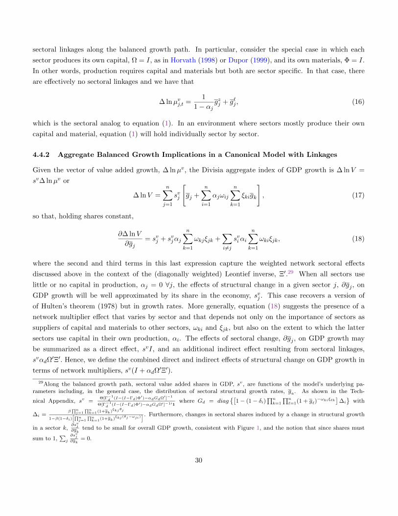
sectoral linkages along the balanced growth path. In particular, consider the special case in which each

sector produces its own capital, Ω = I, as in Horvath (1998) or Dupor (1999), and its own materials, Φ = I.

In other words, production requires capital and materials but both are sector specific. In that case, there

are effectively no sectoral linkages and we have that

∆ lnµvj,t =1

1− αjgzj + g`j , (16)

which is the sectoral analog to equation (1). In an environment where sectors mostly produce their own

capital and material, equation (1) will hold individually sector by sector.

4.4.2 Aggregate Balanced Growth Implications in a Canonical Model with Linkages

Given the vector of value added growth, ∆ lnµv, the Divisia aggregate index of GDP growth is ∆ lnV =

sv∆ lnµv or

∆ lnV =n∑j=1

svj

[gj +

n∑i=1

αjωij

n∑k=1

ξkigk

], (17)

so that, holding shares constant,

∂∆ lnV

∂gj= svj + svjαj

n∑k=1

ωkjξjk +∑i 6=j

sviαi

n∑k=1

ωkiξjk, (18)

where the second and third terms in this last expression capture the weighted network sectoral effects

discussed above in the context of the (diagonally weighted) Leontief inverse, Ξ′.29 When all sectors use

little or no capital in production, αj = 0 ∀j, the effects of structural change in a given sector j, ∂gj , on

GDP growth will be well approximated by its share in the economy, svj . This case recovers a version of

of Hulten’s theorem (1978) but in growth rates. More generally, equation (18) suggests the presence of a

network multiplier effect that varies by sector and that depends not only on the importance of sectors as

suppliers of capital and materials to other sectors, ωki and ξjk, but also on the extent to which the latter

sectors use capital in their own production, αi. The effects of sectoral change, ∂gj , on GDP growth may

be summarized as a direct effect, svI, and an additional indirect effect resulting from sectoral linkages,

svαdΩ′Ξ′. Hence, we define the combined direct and indirect effects of structural change on GDP growth in

terms of network multipliers, sv(I + αdΩ′Ξ′).

29Along the balanced growth path, sectoral value added shares in GDP, sv, are functions of the model’s underlying pa-rameters including, in the general case, the distribution of sectoral structural growth rates, ga. As shown in the Tech-

nical Appendix, sv =Θ[Γ−1

d(I−(I−Γd)Φ′)−αdGdΩ′]−1

Θ[Γ−1d

(I−(I−Γd)Φ′)−αdGdΩ′]−1′1where Gd = diag

[1 − (1 − δi)

∏nk=1

∏n`=1(1 + g`)

−ωkiξ`k]

∆i

with

∆i =β∏nj=1

∏nk=1(1+gk)

ξkjθj

1−β(1−δi)[∏n

j=1

∏nk=1

(1+gk)ξkj(θj−ωji)

] . Furthermore, changes in sectoral shares induced by a change in structural growth

in a sector k,∂svj∂gk

tend to be small for overall GDP growth, consistent with Figure 1, and the notion that since shares must

sum to 1,∑j

∂svj∂gk

= 0.

30

Table 7: Sectoral Network Multipliers

Sector sv svαdΩ′Ξ′ sv (I + αdΩ

′Ξ′)

Agriculture 0.03 0.01 0.03Mining 0.02 0.03 0.05Utilities 0.02 0.01 0.03Construction 0.05 0.12 0.17Durable goods 0.13 0.28 0.42Nondurable goods 0.09 0.03 0.13Wholesale trade 0.07 0.08 0.15Retail trade 0.08 0.02 0.11Trans. & Ware. 0.04 0.03 0.07Information 0.05 0.03 0.08FIRE (x-Housing) 0.10 0.03 0.14PBS 0.09 0.16 0.25Educ. & Health 0.06 0.00 0.06Arts, Ent., & Food svc. 0.04 0.01 0.04Oth. serv. (x-Gov) 0.03 0.01 0.04Housing 0.09 0.00 0.09

Notes: This table decomposes each sector’s total multiplier (column 3) into a direct effect(column 1) and an indirect effect (column 2). The sums do not necessarily add up because ofrounding.

Table 7 shows the direct and combined effects of structural change in the different sectors we consider

on GDP growth given Tables 4 and 5. The importance of Construction and Durable Goods as suppliers

of investment goods results in their having not only a large value added share in GDP, 5 and 13 percent

respectively, but also in their having large spillover effects on other sectors. In particular, the network

multipliers for the Construction and Durable Goods sectors come out to more than 3 times their share,

0.17 and 0.42 respectively. Considering that trend TFP growth in Construction fell by nearly 5 percentage

points between 1950 and 2016 in Figure 3, this gives us, all else equal, a roughly 0.7 percentage point effect

on trend GDP growth from TFP changes in Construction alone. In practice, the aggregate growth effects

from combined changes in TFP and labor in Construction are likely smaller since labor growth has been

moderately positive in that sector throughout the post-war. Nevertheless, the effect from Construction is

large not only because of its central role as a producer of capital, including commercial and residential

structures for all sectors, but also because capital depreciates only partially in any given year. It is apparent

from Table 7 that the effects of structural change on GDP growth are always at least as large as sectoral

shares. The sectoral network multipliers roughly double the share of Professional and Business Services, from

0.09 to 0.25, and Wholesale Trade from 0.07 to 0.15. In other sectors, such as Agriculture, Forestry, Fishing

and Hunting, Entertainment and Food Services, or Housing, the network multipliers are small or negligible

31

as suggested by the corresponding columns of the weighted Leontief inverse. Because the same network

relationships embodied in the Capital Flow table, Ω, and Make-Use table, Φ, determine the importance

that sectors have in the economy both as a share of value added and through their spillover effects, sectors

with relatively larger shares in GDP will also tend to be associated with large network multipliers.

A key implication of Table 7 is that the effects of sectoral change on GDP growth arise in part through a

composition effect. Therefore, secular changes in GDP growth can take place without observable changes in

aggregate TFP growth. For example, consider purely idiosyncratic changes in TFP growth, ∂gzj , that leave

aggregate TFP growth unchanged,∑n

j=1 svj∂g

zj = 0. Despite aggregate TFP growth not changing, these

idiosyncratic changes may nevertheless have an effect on GDP growth since the sum of sectoral multipliers

is larger than 1.

Finally, we return to Table 2 and the calculation in Section 3.2, but this time using the expression

derived for the economy with production linkages across multiple sectors, equation (17). In this expression,

we continue to use the numbers in Table 2, specifically the second and third columns for gzj and g`j , the

fourth column for svj , together with the BEA estimates of αd, Γd, Ω′ and Φ′. Using these estimates, equation

(17) now gives a growth rate for GDP that jumps to 2.97 percent compared to 2.42 percent in the aggregate

one-sector model and 3.24 percent in the data.

Evidently, the balanced growth equations (1), (14), and (17) hold only in the steady state and ignore

important endogenous dynamics driven by capital accumulation. In other words, these equations all miss

dynamic terms that capture deviations from steady state growth. Thus, we now turn our attention to the

model solution and associated Markov decision and policy rules.

5 Quantitative Findings

Having described the balanced growth path implications of sectoral structural change, we now interpret the

secular trend in aggregate GDP growth estimated in Section 2 as part of a slow-moving transition towards

a balanced growth path. Therefore, to assess how sectoral trends in different sectors play out in other

sectors over time, as well as in terms of overall GDP growth, we first work out the transition dynamics of

the model. Given the economy’s balanced growth path, we normalize the model’s variables by appropriate

factors (these are also the factors used in Appendix C) so as to make the model’s optimality conditions and

resource constraints stationary in the detrended variables. The scaling factors used in detrending differ with

the variables under consideration but always involve the entire distribution of growth rates summarized in

ga. Detrended variables are constant along the balanced growth path and while consumption, investment,

materials, and gross output all grow at the same rate within each sector, these variables grow at different

rates across sectors. Prices in different sectors, as well as their implied price indices, also all grow at different

rates along the balanced growth path but in such a way as to generate constant shares along that path. After

linearizing the model’s dynamic equations around the steady state in detrended variables, Markov decision

and policy rules may be readily obtained using standard linear rational expectations solution toolkits,

32

including in this case King and Watson (2002).30

5.1 Historical Decompositions

In exploring the aggregate implications of structural change in individual sectors, the previous section

highlighted the importance of accounting for production linkages and their network effects. In other words,

in any counterfactual exercise, individual sectors cannot be modeled in isolation. In this section, we wish to

recover the dynamic implications of the model for sectoral value added growth, ∆ ln vj,t, and aggregate GDP

growth, ∆ lnVt =∑n

j=1 svj∆ ln vj,t, when driven by the different sectoral processes estimated in Section 3.

In Appendix D, we show that during transitions to the balanced growth path, the vector of value added

growth rates, ∆ ln vt, evolves according to

∆ ln vt =(I + αdΩ

′Ξ′)ga + αd∆kt + At + αdΩ

′Ξ′At−1, (19)

where the vector kt = (k1,t, ..., kn,t)′ denotes the log deviations of detrended capital from its appropriate

level and At = (A1,t, ..., An,t)′ with Aj,t = ∆ lnAj,t− gj . The vector kt follows from the model’s equilibrium

Markov decision rules and is thus a function of previous endogenous states, kt−1, and the various shocks

affecting the economy (i.e. persistent and transitory, as well as idiosyncratic and common). The first term

on the right-hand side of (19) captures the sectoral steady state growth paths described in equation (14).

The additional terms represent the dynamics of value added growth induced by the driving processes, At,

and by endogenous adjustments to capital in different sectors, ∆kt. In the absence of shocks, ∆kt and At

are zero in the long run and ∆ ln vt = (I + αdΩ′Ξ′) ga as in equation (14).

Equation (19) implies both contemporaneous and lagged effects of structural changes, At, on sectoral

value added growth, ∆ ln vt, towards balanced growth. The contemporaneous effect of a structural change in

sector j, ∂∆ lnAj,t, on its own value added, ∆ ln vj,t, is one-for-one whereas this effect is zero on value added

growth in other sectors. It follows that in the period in which a sector experiences a structural change, the

effect of that change on GDP growth is entirely captured by that sector’s share in GDP, ∂∆ lnVt∂∆ lnAj,t

= svj .

Thus, a version of Hulten’s theorem (1978) holds in growth rates on impact.

In subsequent periods, the change in GDP growth stemming from sectoral structural changes will reflect

the network effects of production linkages, svαdΩ′Ξ′∆ lnAt. Along transitions, structural changes will also

affect GDP growth indirectly in-so-far as they are reflected by endogenous changes in the capital stock of

different sectors, svαd∆kt, through optimal investment decisions.

Before assessing the effects of structural changes in individual sectors, we discuss the dynamic model’s

behavior when driven by the processes estimated in Section 3. Relative to the empirical model in that

section, the structural model adds two key features: a rich network of production linkages in both materials

and capital, and endogenous dynamics by way of capital accumulation. Figure 7 illustrates the behavior of

30For a detailed description of this sequence of steps and all their subsequent implications for this section, see the TechnicalAppendix.

33

Figure 7: Sectoral Value-Added Growth Rates Data and Model(Percentage points at an annual rate)

1960 1980 2000 2020

-20

0

20

Agriculture

1960 1980 2000 2020-20

0

20Mining

1960 1980 2000 2020-20

0

20Utilities

1960 1980 2000 2020

0

5

10Construction

1960 1980 2000 2020

0

5

10Durable goods

1960 1980 2000 2020-10

0

10

Nondurable goods

1960 1980 2000 2020-10

0

10

Wholesale trade

1960 1980 2000 2020-5

0

5

10Retail trade

1960 1980 2000 2020-5

0

5

10Trans. & Ware.

1960 1980 2000 2020-10

-5

0

5

10Information

1960 1980 2000 2020-10

-5

0

5

10

FIRE (x-Housing)

1960 1980 2000 2020

0

5

10PBS

1960 1980 2000 2020

0

5

10Educ. & Health

1960 1980 2000 2020

0

5

10

Arts, Ent., & Food svc.

1960 1980 2000 2020-10

0

10Other services (x-Gov)

1960 1980 2000 20200

2

4

6

Housing

Data (Cyclically Adjusted) Model-Implied Growth Rates

Notes: The figure shows the growth rate in value added for each sector. The model-implied value added is computedfrom equation (19) with values of Aj,t from the DFM model.

value added growth in each sector, ∆ ln vj,t, in the data and in the model. As the figure makes clear, the

model performs remarkably well in capturing sectoral value added growth simultaneously across virtually

every sector. The fit is particularly close in some key sectors highlighted above, such as Construction and

Durable Goods, as well as most other sectors. The model misses somewhat on the dynamics of Wholesale

34

Figure 8: GDP Growth - Data and Model

1950 1960 1970 1980 1990 2000 2010 2020-2

0

2

4

6

8A: Growth Rates

Cyclically Adjusted DataBenchmark ModelBalanced Growth Approximation

1950 1960 1970 1980 1990 2000 2010 20200

1

2

3

4

5B: Trends

Cyclically Adjusted Data, 15-Year Centered MABenchmark ModelBalanced Growth Approximation

Notes: Panel (A) shows share-weighted value added growth rates from Figure 7. Panel (B) shows 15-year centeredmoving averages from panel (A) (thin black line) and the model-implied values of growth rates using equation (19)and the τ -components of Aj,t. The dashed lines are balanced growth approximations using equation (17) but withthe disturbances to TFP and labor growth in place of gj .

Trade in the early part of the sample.

In Figure 7, a downward trend is clearly noticeable in Construction more than in any other sector.

This feature of the data is significant in that the Construction sector was also associated with a large

35

multiplier in the previous section. This large multiplier in turn reflected the importance of that sector in

producing capital (commercial and residential structures as well as equipment) for almost every sector in the

economy. A downward trend is also noticeable in Professional and Business Services though considerably

less pronounced.

Figure 8A illustrates the behavior of GDP growth in the model and in the data. The red line depicts

the growth rate of GDP as approximated by the balanced growth formula in equation (17) but driven by

the full set of disturbances to TFP and labor growth in place of gj in that equation. In other words, the

red line shows the model’s predicted GDP growth rate implied by the dynamics embodied in the exogenous

driving processes but absent any internal (endogenous) dynamics from the model. The figure shows that

this predicted growth rate is able to move ‘locally’ with the data. However, it is also considerably more

volatile than actual GDP growth. In contrast, the blue line depicts the behavior of GDP growth in the full

model as implied by the law of motion for sectoral value added growth in equation (19) together with the

Markov decision rules for kt. This line is considerably smoother and closely matches the actual behavior of

GDP growth (in black). The model underpredicts GDP growth slightly in the late 1990s and overstates the

level of GDP growth somewhat in the 2000s but it matches its overall rate of decline almost exactly during

the latter period.

Figure 8B illustrates the implications of the dynamic multi-sector model for trend GDP growth. Specifi-

cally, it illustrates the model’s solution when driven only by the disturbances associated with the persistent

components of labor and TFP growth, ∆τxc,t and ∆τxj,t, x = `, z. The red line represents the trend growth

rate implied by the balanced growth approximation (17) when driven only by these shocks. The blue line in

Figure 8B is the model-implied trend growth rate of GDP taking into account the model’s internal dynam-

ics. The black line depicts a 15−year centered moving average of actual (cyclically adjusted) GDP growth.

The full model indicates that trend GDP growth rate has steadily declined by about 2.2 percent over the

post-war period. In the next sections, therefore, we unpack this slow decline in GDP growth in terms of the

history experienced by individual sectors through counterfactual exercises.

5.2 Implications of Changing Sectoral Trends for GDP Growth

The multi-sector balanced growth model of Section 4 provides an accounting framework for decomposing

the changes in the trend growth rate of GDP shown in Figure 8B into sources associated with common and

sector-specific shocks. More precisely, using equation (19) and the definition of At, the model-based trend

in GDP growth rates can be written as its balanced growth value, say µ∆V , and a distributed-lag of past

trend shocks:

∆ lnVt = µ∆V +[βc,z(L)∆τ zc,t + βc,`(L)∆τ `c,t

]+

n∑j=1

[βj,z(L)∆τ zj,t + βj,`(L)∆τ `j,t

], (20)

where the distributed lag coefficients, β(L), are functions of the model parameters and the factor loadings

that link the common shocks to the sectors. Figure 9 plots the historical contribution of each sector to

36

Figure 9: Model-Based Historical Decomposition of Trend GDP Growth Rates:Contributions from Sector-Specific Trends

1960 1980 2000 20200

0.02

0.04Agriculture

1960 1980 2000 2020-0.1

0

0.1Mining

1960 1980 2000 2020

-0.04

-0.02

0Utilities

1960 1980 2000 2020

-0.6

-0.4

-0.2

0Construction

1960 1980 2000 2020

-0.4

-0.2

0

0.2Durable goods

1960 1980 2000 2020-0.4

-0.2

0Nondurable goods

1960 1980 2000 2020-0.05

0

0.05

0.1Wholesale trade

1960 1980 2000 2020-0.1

-0.05

0

0.05Retail trade

1960 1980 2000 2020-0.15

-0.1

-0.05

0Trans. & Ware.

1960 1980 2000 2020-0.1

-0.05

0

0.05Information

1960 1980 2000 2020

-0.1

-0.05

0FIRE (x-Housing)

1960 1980 2000 2020-0.4

-0.3

-0.2

-0.1

0PBS

1960 1980 2000 2020-0.1

0

0.1

Educ. & Health

1960 1980 2000 2020

0

0.01

0.02

Arts, Ent., & Food svc.

1960 1980 2000 2020-0.05

0

0.05Other services (x-Gov)

1960 1980 2000 2020-0.1

-0.05

0Housing

Notes: These figures show the effect of the sector-specific trend shocks (∆τzj,t and ∆τ `j,t) on the growth rate of GDPusing the model-based dynamic multipliers. The trend growth rates are normalized to 0 in 1950.

∆ lnVt, that is ζj,t = βj,z(L)∆τ zj,t + βj,`(L)∆τ `j,t; Figure 13 plots the contribution of the common shocks,

ζc,t = βc,z(L)∆τ zc,t + βc,`(L)∆τ `c,t (in each figure, pre-sample values of ∆τ are set to zero, so initial values of

ζ are equal to zero.)

The sectoral results shown in Figure 9 suggest that, over the entire post-war period, the Construction

sector is the largest single source of decline in trend GDP growth at approximately 0.6 percentage points.

37

That is, more than 25 percent of the trend decline in GDP growth in the last 60 years is associated with this

sector alone. Other sectors that contributed materially to the fall in trend GDP growth in the last 6 decades

include Professional and Business Services and Nondurable Goods with both sectors contributing more than

0.3 percentage point loss. The Durable Goods sector contributed large decade-long up-and-down swings in

trend GDP growth between 1950 and the end of the sample. The most-recent upswing in Durable Goods,

contributing by itself almost 0.5 percentage points to trend GDP growth between the late 1980s and 2000,

partly reflects technical progress in the production of semiconductors that was much publicized during that

period. The subsequent decrease in Durable Goods accounts for nearly half (0.7 percentage points) of the

1.5 percentage point post-1999 decline in the growth rate of GDP seen in Figure 8B. Finally, some sectors,

such as Information and Wholesale Trade, have somewhat offset the longer run decrease in GDP growth.

Figure 10 looks more closely at the aggregate effects of structural change in the construction sector. Panel

A shows the composite effect of construction-specific changes in trend values of labor and TFP that was

shown previously in Figure 9. Panels B and C show the separate effects from labor (βj,`(L)∆τ `j,t) and TFP

(βj,z(L)∆τ zj,t). Evidently, decreases in the rate of growth of TFP in the construction sector explain most of

its deleterious effect on trend GDP growth. Of course, one interpretation of these historical decompositions

is as counterfactual paths of GDP growth setting all other shocks to zero. In this interpretation, Panel A

of Figure 10 shows the path of the trend growth rate of GDP under the counterfactual absence of changes

in common and sector-specific shocks other than construction (∆τ zc,t = ∆τ `c,t = τ zj,t = ∆τ `j,t = 0 for j 6=Construction). This interpretation of Figure 10 raises the question of how to account for the reduction in

labor associated with ∆τ `j,t in the construction sector. Did it disappear, as implicitly assumed in Panels A

and C, or did it move to other sectors? Panel D shows the counterfactual historical path of trend growth rates

in GDP after allocating all of the sectoral losses of labor in Construction to the other sectors in proportion

to their labor shares, so there is no change in the aggregate supply of labor.31 Because the behavior of labor

growth is not the dominant force driving secular changes in the Construction sector, panels A and D show

similar historical paths.

Figures 11 and 12 repeat this exercise for two other important sectors: Nondurable Goods and Profes-

sional and Business Services. Taken together, Figures 11 and 12 underscore the importance of sector-specific

structural change for trend GDP growth. Remarkably, the Construction, Nondurable Goods, and Profes-

sional and Business Services sectors account for around 60 percent of the 2.2 percentage point decrease in

trend GDP growth since 1950.

In contrast, Figure 13 illustrates the implications of the common or aggregate trends in labor and TFP

growth estimated in Section 4. Figure 13 suggests that these common trends have not made a material

contribution to the aggregate trend decline in GDP growth since 1950. Thus, sector-specific rather than

aggregate factors shaped the major part of the secular behavior of GDP growth over the period 1950−2016.

31Recall also our discussion of the limits on cross-sectoral substitution of KLEMS sectoral labor measures in footnote 19.

38

Figure 10: Model-Based Historical Decomposition of Trend Growth Rates:Contributions from Construction

1950 1960 1970 1980 1990 2000 2010 2020-1

-0.8

-0.6

-0.4

-0.2

0

0.2A: TFP and Labor

1950 1960 1970 1980 1990 2000 2010 2020-1

-0.8

-0.6

-0.4

-0.2

0

0.2B: TFP

1950 1960 1970 1980 1990 2000 2010 2020-0.25

-0.2

-0.15

-0.1

-0.05

0

0.05

0.1C: Labor

1950 1960 1970 1980 1990 2000 2010 2020-1

-0.8

-0.6

-0.4

-0.2

0

0.2D: TFP and Labor with Labor Reallocation

Notes: Panels (A)-(C) show the effect of the sector-specific trend shocks (∆τzj,t and ∆τ `j,t) on the growth rate of GDPusing the model-based dynamic multipliers. Panel (D) shows these effects after reallocating ∆τ `j,t to the other sectors.Blue dots indicate 68 percent credible intervals conditional on balanced growth model parameters. The trend growthrates are normalized to 0 in 1950.

5.3 Implications for Future Trend Growth

Given the trends in labor growth and TFP growth estimated in this paper, and their implications for the

aggregate U.S. economy through sectoral multipliers, a natural question is: what do those trends imply

going forward? As indicated by equation (19), disturbances to trend labor growth and TFP growth are

39

Figure 11: Model-Based Historical Decomposition of Trend Growth Rates:Contributions from Nondurable Goods

1950 1960 1970 1980 1990 2000 2010 2020-0.6

-0.5

-0.4

-0.3

-0.2

-0.1

0

0.1

0.2A: TFP and Labor

1950 1960 1970 1980 1990 2000 2010 2020-0.5

-0.4

-0.3

-0.2

-0.1

0

0.1B: TFP

1950 1960 1970 1980 1990 2000 2010 2020-0.2

-0.15

-0.1

-0.05

0

0.05C: Labor

1950 1960 1970 1980 1990 2000 2010 2020-0.4

-0.3

-0.2

-0.1

0

0.1

0.2D: TFP and Labor with Labor Reallocation

Notes: See notes to Figure 10.

endogenously propagated over time through investment decisions and thus have persistent effects. The

random walk dynamics of the trend components of labor growth and TFP growth imply that forecasts of

these components are equal to their value in 2016, the last year of the data.

Figure 14 shows predicted trend growth rates for GDP from the dynamic multi-sector model as past

disturbances play out through the model’s internal dynamics. The figure indicates that absent the realization

of positive and persistent disturbances to TFP and labor growth, trend GDP growth will continue to fall by

40

Figure 12: Model-Based Historical Decomposition of Trend Growth Rates:Contributions from Professional and Business Services

1950 1960 1970 1980 1990 2000 2010 2020-0.8

-0.6

-0.4

-0.2

0

0.2A: TFP and Labor

1950 1960 1970 1980 1990 2000 2010 2020-0.8

-0.6

-0.4

-0.2

0

0.2B: TFP

1950 1960 1970 1980 1990 2000 2010 2020-0.2

-0.1

0

0.1

0.2

0.3C: Labor

1950 1960 1970 1980 1990 2000 2010 2020-0.8

-0.6

-0.4

-0.2

0

0.2D: TFP and Labor with Labor Reallocation

Notes: See notes to Figure 10.

around 0.60 percentage points over the next 10 years. In this scenario, both trend labor and TFP growth

remain constant, but the internal dynamics of capital accumulation imply continued slowing of trend GDP

growth. The 68 percent credible bands indicate there is substantial uncertainty about the exact level of

trend GDP going forward but, absent positive shocks, the model predicts a slowdown ahead nonetheless.

Table 8 shows the contributions of the common and sector-specific trend components in generating the

decline in trend GDP growth of around 0.65 percentage points going forward. While there is a role for

41

Figure 13: Model-Based Historical Decomposition of Trend Growth Rates:Contributions from Common Trends

1950 1960 1970 1980 1990 2000 2010 2020-1

-0.5

0

0.5

1

1.5

Notes: This figure show the effect of the common trend shocks (∆τzc,t and ∆τ `c,t ) on the growth rate of GDP usingthe model-based dynamic multipliers. Blue dots indicate 68 percent credible intervals conditional on balanced growthmodel parameters. The trend growth rates are normalized to 0 in 1950.

common trends, they play a smaller role than the sector-specific trends, particularly in TFP growth. The

decomposition into each individual sector shows that a decline in Durable Goods is the key driver of lower

trend GDP growth in the future. The fall in large part reflects the propagation of the collapse associated

with the Durable Goods sector that began in 2000 (see Figure 9). This effect is mitigated somewhat by

a turn-around in Construction. However, the marked slowdown in Durable Goods affects other sectors

42

Figure 14: In-Sample and Predicted Out-of-Sample Trend Growth Rate of GDP

1950 1960 1970 1980 1990 2000 2010 2020 2030 20400

0.5

1

1.5

2

2.5

3

3.5

4

4.5

5

Notes: Blue dots indicate 68 percent credible intervals conditional on balanced growth model parameters.

through production linkages, and through capital accumulation implies a pervasive impact that is sustained

10 years into the future.

6 Concluding Remarks

In this paper, we estimate trends in TFP and labor growth across major U.S. production sectors and

explore the role they have played in shaping the secular behavior of GDP growth. We find that trends in

43

Table 8: Model-based Forecasts of Changes in Trend GDP Growth

2016− 2021 2021− 2026

VA Labor TFP VA Labor TFP

Aggregate -0.49 -0.15 -0.34 -0.16 -0.03 -0.13

Common -0.16 -0.05 -0.11 -0.03 0.00 -0.04

Sector specific (total) -0.33 -0.10 -0.23 -0.13 -0.03 -0.10

Sector specific (by sector)

Agriculture -0.00 -0.00 0.00 -0.00 -0.00 -0.00

Mining -0.02 -0.01 -0.01 -0.01 -0.00 -0.00

Utilities -0.00 -0.00 0.00 -0.00 -0.00 0.00

Construction 0.02 -0.01 0.02 0.01 -0.00 0.01

Durable goods -0.31 -0.08 -0.22 -0.12 -0.03 -0.09

Nondurable goods 0.00 0.00 0.00 0.00 -0.00 0.00

Wholesale trade -0.01 -0.00 -0.00 -0.00 -0.00 -0.00

Retail trade 0.00 0.00 0.00 -0.00 0.00 -0.00

Trans. & Ware. -0.00 -0.00 -0.00 -0.00 -0.00 -0.00

Information -0.00 -0.00 0.00 0.00 -0.00 0.00

FIRE (x-Housing) -0.00 0.00 -0.00 -0.00 0.00 -0.00

PBS -0.00 -0.00 -0.00 -0.00 -0.00 -0.00

Educ. & Health -0.00 0.01 -0.01 -0.00 0.00 -0.01

Arts, Ent., & Food svc. -0.00 -0.00 0.00 0.00 -0.00 0.00

Oth. serv. (x-Gov) 0.00 0.00 0.00 0.00 0.00 0.00

Housing -0.01 0.00 -0.01 -0.00 0.00 -0.00

TFP and labor growth have generally decreased across a majority of sectors since 1950. More than 3/4

of the secular decline in aggregate TFP growth results from the combination of sector-specific rather than

aggregate disturbances. Similarly, trend labor growth has also been dominated by sector-specific factors,

especially after 1980 and the latter part of the post-war period.

We embed these findings into a dynamic multi-sector framework in which materials and capital used

by different sectors are produced by other sectors. The presence of capital, in particular, allows changes

in TFP or labor growth in a given sector to affect value added growth in every other sector. This feature

leads to quantitatively important sectoral multiplier effects on GDP growth that reflect the importance of

different sectors as suppliers of capital or materials to other sectors. The strength of these linkages result

44

in GDP growth multipliers that for some sectors can be as large 3 times their value added share.

Ultimately, sector-specific rather than aggregate factors in TFP and labor growth explain the major part

of low frequency variations in U.S. GDP growth. Changing sectoral trends in the last 6 decades, translated

through the economy’s production network, have on net lowered trend GDP growth by around 2.2 percentage

points. The Construction sector, more than any other sector, stands out for its contribution to the trend

decline in GDP growth over the post-war period, accounting for 30 percent of this decline. Moreover, the

process of capital accumulation means that these structural changes have endogenously persistent effects.

Thus, absent the realization of predominantly positive and persistent disturbances to TFP and labor growth,

we estimate that trend GDP growth will continue to fall over the next 10 years.

45

References

Acemoglu, D., V. M. Carvalho, A. Ozdaglar, and A. Tahbaz-Salehi (2012). The Network Origins of Aggregate

Fluctuations. Econometrica 80 (5), 1977–2016.

Acemoglu, D., A. Ozdaglar, and A. Tahbaz-Salehi (2017). Microeconomic Origins of Macroeconomic Tail

Risks. American Economic Review 107 (1), 54–108.

Aghion, P., A. Bergeaud, T. Boppart, P. J. Klenow, and H. Li (2017). Missing Growth from Creative

Destruction. Working Paper Series 2017-4, Federal Reserve Bank of San Francisco.

Atalay, E. (2017). How Important Are Sectoral Shocks? American Economic Journal: Macroeconomics 9 (4),

254–280.

Atalay, E., T. Drautzburg, and Z. Wang (2018). Accounting for the Sources of Macroeconomic Tail Risks.

Economics Letters 165 (C), 65–69.

Baqaee, D. R. (2018). Cascading Failures in Production Networks. Econometrica 86 (5), 1819–1838.

Baqaee, D. R. and E. Farhi (2017a). Productivity and Misallocation in General Equilibrium. NBER Working

Papers 24007, National Bureau of Economic Research, Inc.

Baqaee, D. R. and E. Farhi (2017b). The Macroeconomic Impact of Microeconomic Shocks: Beyond Hulten’s

Theorem. NBER Working Papers 23145, National Bureau of Economic Research, Inc.

Baqaee, D. R. and E. Farhi (2018). The Microeconomic Foundations of Aggregate Production Functions.

NBER Working Papers 25293, National Bureau of Economic Research, Inc.

Barkai, S. (2017). Declining Labor and Capital Shares. Mimeo.

Basu, S. and J. Fernald (2001). Why Is Productivity Procyclical? Why Do We Care? In New Developments

in Productivity Analysis, NBER Chapters, pp. 225–302. National Bureau of Economic Research, Inc.

Basu, S. and J. G. Fernald (1997). Returns to Scale in U.S. Production: Estimates and Implications. Journal

of Political Economy 105 (2), 249–283.

Basu, S., J. G. Fernald, J. Fisher, and M. S.Kimball (2013). Sector-Specific Technical Change. Mimeo.

Bigio, S. and J. La‘O (2016). Financial Frictions in Production Networks. NBER Working Papers 22212,

National Bureau of Economic Research, Inc.

Byrne, D. M., J. G. Fernald, and M. B. Reinsdorf (2016). Does the United States Have a Productivity

Slowdown or a Measurement Problem? Brookings Papers on Economic Activity 47 (1 (Spring), 109–182.

46

Cette, G., J. Fernald, and B. Mojon (2016). The Pre-Great Recession Slowdown in Productivity. European

Economic Review 88 (C), 3–20.

Cummins, J. G. and G. L. Violante (2002). Investment-Specific Technical Change in the US (1947-2000):

Measurement and Macroeconomic Consequences. Review of Economic Dynamics 5 (2), 243–284.

De Loecker, J. and J. Eeckhout (2017). The Rise of Market Power and the Macroeconomic Implications.

NBER Working Papers 23687, National Bureau of Economic Research, Inc.

Decker, R. A., J. Haltiwanger, R. S. Jarmin, and J. Miranda (2016). Where has All the Skewness Gone?

The Decline in High-Growth (Young) Firms in the U.S. European Economic Review 86 (C), 4–23.

di Giovanni, J., A. A. Levchenko, and I. Mejean (2014). Firms, Destinations, and Aggregate Fluctuations.

Econometrica 82 (4), 1303–1340.

Dupor, B. (1999). Aggregation and Irrelevance in Multi-Sector Models. Journal of Monetary Eco-

nomics 43 (2), 391–409.

Fernald, J. G. (2014). Productivity and Potential Output before, during, and after the Great Recession.

NBER Macroeconomics Annual 29 (1), 1–51.

Fernald, J. G., R. E. Hall, J. H. Stock, and M. W. Watson (2017). The Disappointing Recovery of Output

after 2009. Brookings Papers on Economic Activity 48 (1), 1–81.

Fernald, J. G. and C. I. Jones (2014). The Future of US Economic Growth. American Economic Re-

view 104 (5), 44–49.

Fleck, S., S. Rosenthal, M. Russell, E. H. Strassner, and L. Usher (2014). A Prototype BEA/BLS Industry-

Level Production Account for the United States, pp. 323–372. University of Chicago Press.

Foerster, A. T., A. Hornstein, P.-D. G. Sarte, and M. W. Watson (2019). “Technical Appendix and Supple-

mentary Material for: Aggregate Implications of Changing Sectoral Trends”.

Foerster, A. T., P.-D. G. Sarte, and M. W. Watson (2011). Sectoral versus Aggregate Shocks: A Structural

Factor Analysis of Industrial Production. Journal of Political Economy 119 (1), 1–38.

Gabaix, X. (2011). The Granular Origins of Aggregate Fluctuations. Econometrica 79 (3), 733–772.

Gordon, R. J. (1990). The Measurement of Durable Goods Prices. National Bureau of Economic Research,

Inc.

Gordon, R. J. (2014). The Demise of U.S. Economic Growth: Restatement, Rebuttal, and Reflections.

NBER Working Papers, National Bureau of Economic Research, Inc.

47

Gordon, R. J. and H. Sayed (2019). The Industry Anatomy of the Transatlantic Productivity Growth

Slowdown. NBER Working Papers, National Bureau of Economic Research, Inc.

Grassi, B. (2018). IO in I-O: Size, Industrial Organization, and the Input-Output Network Make a Firm

Structurally Important. Working Papers 619, IGIER (Innocenzo Gasparini Institute for Economic Re-

search), Bocconi University.

Greenwood, J., Z. Hercowitz, and P. Krusell (1997). Long-Run Implications of Investment-Specific Techno-

logical Change. American Economic Review 87 (3), 342–362.

Horvath, M. (1998). Cyclicality and Sectoral Linkages: Aggregate Fluctuations from Independent Sectoral

Shocks. Review of Economic Dynamics 1 (4), 781–808.

Horvath, M. (2000). Sectoral Shocks and Aggregate Fluctuations. Journal of Monetary Economics 45 (1),

69–106.

Hulten, C. R. (1978). Growth Accounting with Intermediate Inputs. Review of Economic Studies 45 (3),

511–518.

Jorgenson, D. W., M. Ho, A. Patel, and J. Samuels (2014). Data Appendix to “Economic Growth in the

Information Age”. Mimeo.

Jorgenson, D. W., M. S. Ho, and J. D. Samuels (2017). Educational Attainment and the Revival of U.S.

Economic Growth, pp. 23–60. University of Chicago Press.

Karabarbounis, L. and B. Neiman (2018). Accounting for Factorless Income. In NBER Macroeconomics

Annual 2018, volume 33, NBER Chapters. National Bureau of Economic Research, Inc.

Kimball, M. S., J. G. Fernald, and S. Basu (2006). Are Technology Improvements Contractionary? American

Economic Review 96 (5), 1418–1448.

King, R. G. and M. W. Watson (2002). System Reduction and Solution Algorithms for Singular Linear

Difference Systems under Rational Expectations. Computational Economics 20 (1-2), 57–86.

Long, John B, J. and C. I. Plosser (1983). Real Business Cycles. Journal of Political Economy 91 (1), 39–69.

McGrattan, E. R. and J. A. Schmitz (1999). Maintenance and Repair: Too Big to Ignore. Federal Reserve

Bank of Minneapolis Quarterly Review Fall, 2–13.

Miranda-Pinto, J. (2019). Production Network Structure, Service Share, and Aggregate Volatility. Working

Paper, University of Queensland 170 (C), 152–156.

Muller, U. K. and M. W. Watson (2018). Long-Run Covariability. Econometrica 86 (3), 775–804.

48

Ngai, L. R. and C. A. Pissarides (2007). Structural Change in a Multisector Model of Growth. American

Economic Review 97 (1), 429–443.

Oliner, S. D., D. E. Sichel, and K. J. Stiroh (2007). Explaining a Productive Decade. Brookings Papers on

Economic Activity 38 (1), 81 – 137.

Rossi-Hansberg, E., P.-D. Sarte, and N. Trachter (2018). Diverging Trends in National and Local Concen-

tration. NBER Working Papers 25066, National Bureau of Economic Research, Inc.

Stock, J. H. and M. W. Watson (2016). Core Inflation and Trend Inflation. The Review of Economics and

Statistics 9 (4), 770 – 784.

Traina, J. (2018). Is Aggregate Market Power Increasing? Production Trends Using Financial Statements.

New Working Paper Series 17, Stigler Center.

Whelan, K. (2003). A Two-Sector Approach to Modeling NIPA Data. Journal of Money, Credit and

Banking 35 (4), 627 – 656.

49

Appendix A: Estimation of the Multivariate Unobserved Components

Model

The DFM has the form: ∆ lnxj,t = λxj,ττxc,t + λxj,εε

xc,t + τxj,t + εxj,t, where x = z or ` and j = 1, ..., n. The τ

components evolve as random walks and the ε components as white noise. More specifically, we assume that

the 2(n+ 1)× 1 vector ζt =(

∆τxc,t, εxc,t, ∆τxj,t, εxj,tnj=1

)is i.i.d. with ζ ∼ N(0,Σζ), where Σζ is a diagonal

matrix. The factor loadings and scale of the common factors are not separately identified; thus we normalize

var(∆τxc,t) = var(εxc,t) = 1,∑n

j=1 λxj,τ ≥ 0, and

∑nj=1 λ

xj,ε ≥ 0 to identify the scale and sign of the factors.

We estimate the model using Bayesian methods. We use independent priors for all the parameters. The

priors for the factor loadings are λxj,τ ∼ N(0, 1) and λxj,ε ∼ N(0, 16). The priors for var(∆τxj,t) and var(εxj,t)

are inverse Gamma priors with shape and scale parameters that correspond to Tprior observations with

s2prior = ω2

prior/Tprior. We use Tprior = 2 and s2prior = 0.252 for var(∆τxj,t) and Tprior = 2 and s2

prior = 3.002

for var(εxj,t).

The posterior is approximated using Gibbs-MCMC methods. Let X denote the data, ζ denote the values

for ζt for t = 1, ..., T , and θ denote the parameter values(λxj,τ , λ

xj,ε, var(∆τ

xj,t), var(ε

xj,t

)for j = 1, ...n. The

first Gibbs step draws ζ|(X, θ) using standard formulae related to the Kalman smoother. The second Gibbs

step draws θ from the posterior of θ|(X, ζ) that is also known in closed form from familiar linear regression

formulae. The estimates reported in the paper rely on one million MCMC draws after 5k initial draws.

The Technical Appendix contains additional details.

Appendix B: The Influence Vector in a Model with Capital

The competitive equilibrium of the economy described in the main text is defined as a set of gross output

prices, pyj,t, value added prices, pvj,t, materials prices, pmj,t, and investment goods prices, pxj,t, for all sectors j

and dates t, and allocations, (cj,t, Ct, xij,t,mij,t, xj,t,mj,t, vj,t, yj,t, kj,t+1, `j,t), such that

i) the representative household maximizes its utility,

ii) the representative firm in each sector maximizes profits

iii) all markets clear.

Absent frictions, equilibrium allocations may be found by solving a planner’s problem whose correspond-

ing decentralization and definitions of prices are straightforward.

Suppose that sectoral structural changes embodied in zj,t, `j,t are stationary in levels, with non-

stochastic steady state denoted by zj , `j. Then, in the absence of shocks, the economy converges to

a steady state in the long-run indexed by A = (A1, ..., An), where lnAj = ln zj + (1− αj) ln `j , j = 1, ..., n.

In the steady state, first-order conditions imply a set of relationships between the prices of materials,

investment, and value added,

Θ ln py = 0,

50

ln pv = Γ−1d

[I − (I − Γd)Φ

′] ln py,

ln px = Ω′ ln py,

where pv = (pv1, ..., pvn)′, px = (px1 , ..., p

xn)′, and py = (py1, ..., p

yn)′.

From the definition of value added, we have that

ln vj = lnAj + αj ln

(kjαj

),

and from the Euler equation governing the optimal choice of capital in each sector,

kjαj

=

(pvjvj

pxj

)(β

1− β(1− δj)

).

Combining these expressions gives

ln vj = lnAj + αj ln(pvjvj

)− αj ln pxj + αj ln

(β

1− β(1− δj)

),

or in matrix form,

(I − αd) ln (pv.× v) = lnA+ ln pv − αd ln px + αd ln ∆d,

where (pv.× v) represents the vector of nominal value added,pvjvj

, αd = diag(αj), and ∆d =

diag(

β1−β(1−δj)

). Substituting for investment and value added prices on the right-hand-side of this last

expression, we obtain

ln py =(Γ−1d

[I − (I − Γd)Φ

′]− αdΩ′)−1[(I − αd) ln (pv.× v)− lnA− αd ln ∆d] . (B.1)

From the resource constraints in each sector j, and the optimal allocation of materials and investment

in the economy, it follows that

pvjvj

γj= θjC +

n∑i=1

φji(1− γj)pvi viγi

+n∑i=1

ωjiβδj

1− β(1− δj)αip

vi vi,

or in matrix form,

Γ−1d (pv.× v) = Θ′C + Φ(I − Γd)Γ

−1d (pv.× v) + Ω∆dδdαd (pv.× v) , (B.2)

so that(pv.× v)

C=([I − Φ(I − Γd)] Γ−1

d − Ω∆dδdαd)−1

Θ′.

51

Aggregate GDP (in units of the final consumption bundle) is then given by

V = 1′ (pv.× v) = 1′ψC,

where ψ =([I − Φ(I − Γd)] Γ−1

d − Ω∆dδdαd)−1

Θ′.

Substituting the expression for value added in (B.2) into the equation for gross output prices, (B.1), and

using the fact that the ideal price index for the final consumption bundle implies Θ ln py = 0, we obtain

lnC =Θ(Γ−1d [I − (I − Γd)Φ

′]− αdΩ′)−1

[lnA+ αd ln ∆d − (I − αd) lnψ]

Θ(Γ−1d [I − (I − Γd)Φ′]− αdΩ′

)−1(I − αd)1

,

where note that Θ(Γ−1d [I − (I − Γd)Φ

′]− αdΩ′)−1

(I − αd)1 = 1.

It follows that∂ lnV

∂ lnAj=

∂ lnC

∂ lnAj=(

[I − Φ(I − Γd)] Γ−1d − Ωαd

)−1Θ′j.

At the same time, the vector of value added shares, sv, is given by

(pv.× v)

V=

([I − Φ(I − Γd)] Γ−1

d − Ω∆dδdαd)−1

Θ′

1′([I − Φ(I − Γd)] Γ−1

d − Ω∆dδdαd)−1

Θ′.

Therefore, in the limit case where β → 1, ∆dδd → I, and

∂ lnV

∂ lnAj= ηsvj ,

where η = 1′([I − Φ(I − Γd)] Γ−1

d − Ωαd)−1

Θ′ is approximately the inverse of the mean labor share across

sectors. To see this, observe that η can also be expressed as η =1′([I−Φ(I−Γd)]Γ−1

d −Ωαd)−1

Θ′

1′(I−αd)([I−Φ(I−Γd)]Γ−1d −Ωαd)

−1Θ′. Thus,

when αj = α ∀j, η = 11−α .

Appendix C: Balanced Growth with Sectoral Linkages in Materials and

Investment

We begin by normalizing some of the model’s key variables with respect to sector-specific factors, µj,t, to

be determined below, so as to yield a system of equations that is stationary in the normalized variables.

If all growth rates are constant, the resource constraint in any individual sector implies that all variables

in that constraint must grow at the same rate along a balanced growth path. Thus, define yj,t = yj,t/µj,t,

52

cj,t = cj,t/µj,t, mji,t = mji,t/µj,t, and xji,t = xji,t/µj,t. Then, the economy’s resource constraint becomes

cj,t +n∑i=1

mji,t +n∑i=1

xji,t = yj,t.

Similarly, the production of investment goods may be re-written as

xj,t =

n∏j=1

(xij,tωij

)ωij,

where xj,t = xj,t/∏nj=1 µ

ωiji,t , while the capital accumulation equation becomes

kj,t+1 = xj,t + (1− δj)kj,tn∏j=1

(µi,t−1

µi,t

)ωij,

where kj,t+1 = kj,t+1/∏nj=1 µ

ωiji,t .

The expression for value added may be written as

vj,t = Aj,t

(kj,t∏nj=1 µ

ωiji,t−1

αj

)αj,

so that, defining vj,t = vj,t/Aj,t

(∏nj=1 µ

ωiji,t−1

)αj, it becomes

vj,t =

(kj,tαj

)αj.

The composite bundle of materials used in sector j may be expressed as

mj,t =n∏j=1

(mij,t

φij

)φij,

with mj,t = mj,t/∏nj=1 µ

φiji,t . Therefore, gross output in terms of detrended variables is given by

yj,tµj,t =

(vj,tAj,t

∏nj=1 µ

αjωiji,t−1

γj

)γj (mj,t

∏nj=1 µ

φiji,t

1− γj

)1−γj

,

or alternatively,

yj,t =

(vj,tγj

)γj ( mj,t

1− γj

)1−γjAγjj,tµj,t

n∏j=1

µγjαjωiji,t−1 µ

(1−γj)φiji,t

.

53

We can now use the expression in square brackets to solve for the normalizing factors, µj,t, as a function of

the model’s underlying parameters.

First, re-write the term in square brackets as

Aγjj,t

µj,t

n∏j=1

µγjαjωiji,t−1

µγjαjωiji,t

n∏j=1

µ(1−γj)φiji,t µ

γjαjωiji,t

,

where this last expression involves the growth rate of µi,t. Then, along a balanced growth path where all

variables grow at constant rates, the termAγjj,t

µj,t

∏nj=1 µ

(1−γj)φiji,t µ

γjαjωiji,t must be constant. Thus, we choose

µj,t such that

Aγjj,t

µj,t

n∏j=1

µγjαjωij+(1−γj)φiji,t = 1.

This choice is without loss of generality since any other constant in place of 1 will be differenced out along

the balanced growth path.

Taking logs of both sides of the above expression, we have

γj lnAj,t − lnµj,t +n∑i=1

(γjαjωij + (1− γj)φij) lnµi,t = 0,

or in vector form,

Γd lnAt − lnµt + ΓdαdΩ′ lnµt + (I − Γd)Φ

′ lnµt = 0,

which gives us

lnµt = Ξ′ lnAt (C.1)

where

Ξ′ =(I − ΓdαdΩ

′ − (I − Γd)Φ′)−1

Γd

is the Leontief inverse, (I − ΓdαdΩ′ − (I − Γd)Φ

′)−1, diagonally weighted by value added shares in gross

output, Γd.

Going back to equation (12) in the main text, and writing the vector of productivity growth rates as

∆ lnAt = ga, it follows that

∆ lnµt = Ξ′ga = Ξ′ (gz + (I − αd)g`) .

Thus, let µvj,t denote the normalizing factor for value added in sector j defined above,

µvj,t = Aj,t

n∏j=1

µωiji,t−1

αj

.

54

Then, using equation (C.1), we have that

lnµvt = lnAt + αdΩ′Ξ′ lnAt−1,

or, along a steady state growth path,

∆ lnµvt =

I + αdΩ′(I − αdΓdΩ′ − (I − Γd)Φ

′)−1Γd︸ ︷︷ ︸

Ξ′

ga. (C.2)

Appendix D: The Dynamics of Value Added Growth

We wish to recover the implications of the model for sectoral value added growth, ∆ ln vj,t, and aggregate

GDP growth, ∆ lnVt.

Observe that

∆ ln vj,t = αj∆ ln kj,t,

and that ∆ ln kj,t = ∆kj,t, where ∆kj,t follows directly from the Markov decision rules. Then, by definition

of vj,t,

∆ ln vj,t = ∆ ln vj,t + ∆ lnAj,t +n∑i=1

αjωij∆ lnµi,t−1

= αj∆kj,t + Aj,t + gj +n∑i=1

αjωij∆ lnµi,t−1,

or, in vector form,

∆ ln vt = αd∆kt + At + ga + αdΩ′∆ lnµt−1.

The sectoral detrending factors, µj,t, solve

∆ lnµt = Ξ′∆ lnAt,

where

Ξ′ =(I − ΓdαdΩ

′ − (I − Γd)Φ′)−1

Γd.

Then,

∆ ln vt = αd∆kt + At + ga + αdΩ′Ξ′(At−1 + ga

)

55

or

∆ ln vt =(I + αdΩ

′Ξ′)ga + αd∆kt + At + αdΩ

′Ξ′At−1,

with ∆ lnVt = sv∆ ln vt. When all shocks are set to zero, so that ∆kt = At = At−1 = 0, we recover the

sectoral balanced growth paths for sectoral value added,

∆ ln vt =(I + αdΩ

′Ξ′)ga.

56