Embed Size (px)
Citation preview
AGENT-BASED MODELING OF RACCOON RABIES EPIDEMIC AND ITS ECONOMIC CONSEQUENCES
DISSERTATION
Completed in Partial Fulfillment of the Requirements for
the Degree Doctor of Philosophy in the Graduate
School of The Ohio State University
By
Pirouz Foroutan, M.A.
The Ohio State University
2003
Dissertation Committee: Professor Mario Miranda, Adviser Approved by Professor Brian Roe _____________________ Adviser Professor Alan Randall
Department of Agricultural, Doctor Martin Meltzer Environmental and Development Economics
ii
ABSTRACT
In the United States, rabies strains that infect raccoons have been responsible for the
largest increase animal rabies in the past 3 decades. This work includes three articles that
analyze: 1) the cost of 8 distributions of oral rabies vaccine (ORV) with strains known to
infect raccoons in Ohio between 1997 and 2000, 2) an agent-based simulation of
uninterrupted raccoon rabies epidemic in a hypothetical area, and 3) the costs and
benefits of different ORV distribution strategies.
Article 1 documents the estimated cost of implementing an ORV program to provide a
more efficient use of resources to control and limit the spread of rabies. Accurately
measured distribution costs can be used to perform an economic cost-benefit analysis for
alternative ORV programs. The existing ORV procedure consists of distributing fishmeal
bait containing ORV through various means. The cost of personnel, vehicles, and
helicopter and aircraft use and other associated expenses were obtained from field records
and interviews with personnel and agencies involved in the ORV program.
Article 2 examines the major characteristics and behavior of raccoon agents and their
relation to their environment. Under different parameter values, the models are simulated
and results of a hypothetical raccoon rabies event is obtained in terms of the rate of
disease movement, shape of the epidemic front and intensity of new infections. The
results indicate that model results are sensitive to certain parameters (e.g., aggressiveness
iii
of the epidemic regime, or nutrient regeneration capability of spatial units). Results on
the shape of epidemic front proved to be invariant to different selection of model
parameters.
In article 3, different ORV distribution strategies were devised to assess the effectiveness
of ORV distribution strategies under different assumptions and their potential costs.
Based on raccoon rabies literature, incidences of new infections were mapped to
economic costs. These costs were used in conjunction with distribution costs obtained in
Article 1 to conduct cost-benefit analyses. Results of cost-benefit analysis indicate while
ORV distribution is not economically justifiable for the scope of hypothetical model
space, the potential for justification of the program in a larger and real space is possible.

iv
Dedicated to Parichehreh Ghafouri
v
ACKNOWLEDGEMENTS
I wish to thank my adviser, Mario Miranda, for his support and encouragement in
my choice of methodology, his guidance throughout the writing of my dissertation, and
his always inspiring sense of humor.
I am grateful to Brian Roe for his significant contribution in reviewing many
drafts of my research, his useful comments, and for persevering with me as my mentor
throughout the time it took me to complete this research and write the dissertation.
I thank Martin Meltzer for his intellect and for sharing with me his vast
knowledge of health economics. I am thankful for his major contribution in writing the
first article of this dissertation and for his continued support in procuring funding for me
throughout my graduate career.
I must also thank Alan Randall for teaching me the importance of critical thinking
and ethical standards as a professional, and for his continued guidance in my research.
I also wish to thank Elena Irwin for introducing me to the field of agent-based
modeling and for her guidance. My thanks go also to Kathleen Smith for providing
valuable information from the Ohio Department of Health, and her major contribution in
the first article of this dissertation.
This work would not have been possible without the continual support of my
wife, Jacquelyn Spangler, and my sisters, Parisa and Pardis, and the inspiration of my
son, Cyrus.
vi
VITA December 28, 1963. . . . . .Born – Bushehr, Iran 2000. . . . . . . . . . . . . . . . . .M.A., Economics, The Ohio State University 1997-2003. . . . . . . . . . . . . Fellow, The Centers for Disease Control and Prevention
Publications
Foroutan, Pirouz. “Costs of Distributing Oral Raccoon Rabies Vaccine in Ohio: 1997-2000,” with Martin I. Meltzer and Kathleen A. Smith, Journal of the American Veterinary Medical Association, 220(2002): 27-32.
Fields of Study
Major Field: Agricultural, Environmental, and Development Economics
vii
TABLE OF CONTENTS
Page Abstract. . . . . . . . . . . . . . . . . . . . . . . . . . . . . . . . . . . . . . . . . . . . . . . . . . . . . . . . . . . . . ii Dedication. . . . . . . . . . . . . . . . . . . . . . . . . . . . . . . . . . . . . . . . . . . . . . . . . . . . . . . . . . . iv Acknowledgements. . . . . . . . . . . . . . . . . . . . . . . . . . . . . . . . . . . . . . . . . . . . . . . . . . . .v Vita. . . . . . . . . . . . . . . . . . . . . . . . . . . . . . . . . . . . . . . . . . . . . . . . . . . . . . . . . . . . . . . . vi List of Tables. . . . . . . . . . . . . . . . . . . . . . . . . . . . . . . . . . . . . . . . . . . . . . . . . . . . . . . .viii List of Figures. . . . . . . . . . . . . . . . . . . . . . . . . . . . . . . . . . . . . . . . . . . . . . . . . . . . . . . xiii Articles: 1. Costs of Distributing Orally Administered Raccoon-Variant
Rabies Vaccine in Ohio: 1997-2000. . . . . . . . . . . . . . . . . . . . . . . . . . . . . . . . . . 1 References: Article 1. . . . . . . . . . . . . . . . . . . . . . . . . . . . . . . . . . . . . . . . . . . . . . . . . . . 15 2. Predicting Movement Of An Infectious Disease: An Agent-Based
Modeling Approach. . . . . . . . . . . . . . . . . . . . . . . . . . . . . . . . . . . . . . . . . . . . . .22 References: Article 2. . . . . . . . . . . . . . . . . . . . . . . . . . . . . . . . . . . . . . . . . . . . . . . . . . . 57 3. Economic Analysis of A Raccoon Rabies Abatement Program:
An Agent-Based Modeling Approach. . . . . . . . . . . . . . . . . . . . . . . . . . . . . . . . 97 References: Article 3. . . . . . . . . . . . . . . . . . . . . . . . . . . . . . . . . . . . . . . . . . . . . . . . . . .112 Bibliography. . . . . . . . . . . . . . . . . . . . . . . . . . . . . . . . . . . . . . . . . . . . . . . . . . . . . . . . .122 Appendix: Basis for the values of ecological and epidemiological parameters
of the model. . . . . . . . . . . . . . . . . . . . . . . . . . . . . . . . . . . . . . . . . . . . . . . . . . . .127
viii
LIST OF TABLES Table Page
1.1 Ohio oral rabies vaccine distribution effort: 1997-2000. . . . . . . . . . . . . . . . 19 1.2 Ground distribution costs of the Ohio oral rabies vaccine (ORV) program . . . . . . . . . . . . . . . . . . . . . . . . . . . . . . . . . . . . . . . . . . . . . . .19 1.3 Air Distribution Costs of the Ohio ORV Program . . . . . . . . . . . . . . . . . . . . 20 1.4 Distribution and Financial Costs of the Ohio ORV Program. . . . . . . . . . . . .21 2.1 Ranking of raccoon habitats. . . . . . . . . . . . . . . . . . . . . . . . . . . . . . . . . . . . . .64 2.2 Models: Article 2. . . . . . . . . . . . . . . . . . . . . . . . . . . . . . . . . . . . . . . . . . . . . . 64 2.3 Average pre-epidemic population densities by land use category. . . . . . . . .65 2.4 Major categories of average population densities for models with Simple nutrient grow back algorithm . . . . . . . . . . . . . . . . . . . . . . . . . . 66 2.5 Major categories of average population densities for models with Urban nutrient grow back algorithm. . . . . . . . . . . . . . . . . . . . . . . . . . . 66 2.6 Comparison of major categories of population densities for models with Simple versus Urban nutrient grow back algorithm . . . . . . . . . . . . . . . 67 2.7 Comparison of major categories of population densities for models with Uniform versus Normal home range distribution: t statistics. . . . . . . . .67 2.8 Comparison of major categories of population densities for pairs of models with uniform versus normal home range distribution: Z statistics. . . . . . . . . . . . . . . . . . . . . . . . . . . . . . . . . . . . . . . . . .68 2.9 Comparison of major categories of population densities for pairs of models with 13-week versus 21-week mating season: Z statistics. . . . . . . . . . . . . . . . . . . . . . . . . . . . . . . . . . . . . . . . . . . . . .68

ix
Table Page 2.10 Consistency of models with Simple nutrient grow back algorithm, uniform home range distribution and 13-week mating season: Z statistics. . . . . . . . . . . . . . . . . . . . . . . . . . . . . . . . . . . . . . . .69 2.11 Consistency of models with Simple nutrient grow back algorithm, uniform home range distribution and 21-week mating season: Z statistics. . . . . . . . . . . . . . . . . . . . . . . . . . . . . . . . . . . . . . . .69 2.12 Consistency of models with Simple nutrient grow back algorithm, normal home range distribution and 13-week mating season: Z statistics . . . . . . . . . . . . . . . . . . . . . . . . . . . . . . . . . . . . . . . .70 2.13 Consistency of models with Simple nutrient grow back algorithm, normal home range distribution and 21-week mating season: Z statistics . . . . . . . . . . . . . . . . . . . . . . . . . . . . . . . . . . . . . . . .70 2.14 Consistency of models with Urban nutrient grow back algorithm, uniform home range distribution and 13-week mating season: Z statistics . . . . . . . . . . . . . . . . . . . . . . . . . . . . . . . . . . . . . . . .71 2.15 Consistency of models with Urban nutrient grow back algorithm, uniform home range distribution and 21-week mating season: Z statistics . . . . . . . . . . . . . . . . . . . . . . . . . . . . . . . . . . . . . . . .71 2.16 Consistency of models with Urban nutrient grow back algorithm, normal home range distribution and 13-week mating season: Z statistics . . . . . . . . . . . . . . . . . . . . . . . . . . . . . . . . . . . . . . . .72 2.17 Consistency of models with Urban nutrient grow back algorithm, normal home range distribution and 21-week mating season: Z statistics . . . . . . . . . . . . . . . . . . . . . . . . . . . . . . . . . . . . . . . .72 2.18 Number of weeks lapsed after onset of rabies until its appearance by quadrant (1 through 8) in models with Simple nutrient grow back algorithm: aggressive vs. non-aggressive epidemic regimes . . . . . . . . . 73 2.19 Number of weeks lapsed after onset of rabies until its appearance by quadrant (1 through 8): in models with Urban nutrient grow back algorithm aggressive vs. non-aggressive epidemic regimes . . . . . . . . . 74 2.20 Order of infection by quadrant (1 through 8) in models with
Simple nutrient grow back algorithm: aggressive vs. non-aggressive epidemic regimes. . . . . . . . . . . . . . . . . . . . . . . . . . . . . . . . . . . . . . . . . . . . . . . 75
x
Table Page 2.21 Order of infection by quadrant (1 through 8) in models with Urban nutrient grow back algorithm: aggressive vs. non-aggressive epidemic regimes. . . . . . . . . . . . . . . . . . . . . . . . . . . . . . . . . . . . . . . . . . . . . . . 76 2.22 Number of infections by quadrant in models with Simple nutrient grow back algorithm: comparison of aggressive vs. non-aggressive epidemic regimes. . . . . . . . . . . . . . . . . . . . . . . . . . . . . . . . . . . . . . . . . . . . . . . 77 2.23 Number of infections by quadrant in models with Urban nutrient grow back algorithm: comparison of aggressive vs. non-aggressive epidemic regimes. . . . . . . . . . . . . . . . . . . . . . . . . . . . . . . . . . . . . . . . . . . . . . . 78 2.24 Number of weeks lapsed after onset of rabies until its appearance by quadrant (1 through 8) in models with aggressive epidemic regime: Simple versus Urban nutrient grow back. . . . . . . . . . . . . . . . . . . . . . 79 2.25 Number of weeks lapsed after onset of rabies until its appearance by quadrant (1 through 8) in models with non-aggressive epidemic regime: Simple versus Urban nutrient grow back . . . . . . . . . . . . . . . . . . . . . .80 2.26 Order of infection by quadrant (1 through 8) in models with aggressive epidemic regime: Simple versus Urban nutrient grow back algorithm. . . . . . 81 2.27 Order of infection by quadrant (1 through 8) in models with non-aggressive epidemic regime: Simple versus Urban nutrient grow back algorithm. . . . . . . . . . . . . . . . . . . . . . . . . . . . . . . . . . . . . . . . . . . . .82 2.28 Number of infections by quadrant in models with aggressive epidemic regime: Simple versus Urban nutrient grow back algorithm. . . . . . . . . . . . . . . . 83 2.29 Number of infections by quadrant in models with non-aggressive epidemic regime: Simple versus Urban nutrient grow back algorithm. . . . . . 84 2.30 Speed of epidemic front in models with aggressive epidemic regime: uniform versus normal home range distribution. . . . . . . . . . . . . . . . . . . . . . . 85 2.31 Speed of epidemic front in models with non-aggressive epidemic regime: uniform versus normal home range distribution . . . . . . . . . . . . . . . .86 2.32 Order of infection by quadrant (1 through 8) in models with aggressive epidemic regime: uniform versus normal home range distribution . . . . . . . . 87

xi
Table Page 2.33 Order of infection by quadrant (1 through 8) in models with non-aggressive epidemic regime: uniform versus normal home range distribution . . . . . . . . . . . . . . . . . . . . . . . . . . . . . . . . . . . . . . . . . . . . . . 88 2.34 Number of infections in models with aggressive epidemic regime: uniform versus normal home range distribution. . . . . . . . . . . . . . . . . . . . . . . 89 2.35 Number of infections in models with non-aggressive epidemic regime: uniform versus normal home range distribution. . . . . . . . . . . . . . . . . . . . . . . 90 2.36 Speed of epidemic front in models with aggressive epidemic regime: 13-week versus 21-week mating season . . . . . . . . . . . . . . . . . . . . . . . . . . . . . 91 2.37 Speed of epidemic front in models with non-aggressive epidemic regime: 13-week versus 21-week mating season . . . . . . . . . . . . . . . . . . . . . . 92 2.38 Order of infection by quadrant (1 through 8) in models with aggressive epidemic regime: 13-week versus 21-week mating season . . . . . . . . . . . . . .93 2.39 Order of infection by quadrant (1 through 8) in models with non- aggressive epidemic regime: 13-week versus 21-week mating season. . . . . .94 2.40 Number of infections in models with aggressive epidemic regime: 13 weeks versus 21 weeks mating season. . . . . . . . . . . . . . . . . . . . . . . . . . . . 95 2.41 Number of infections in models with non-aggressive epidemic regime: 13 weeks versus 21 weeks mating season. . . . . . . . . . . . . . . . . . . . . . . . . . . . 96 2.42 Summary of effects of model variables with respect to speed and shape of epidemic front . . . . . . . . . . . . . . . . . . . . . . . . . . . . . . . . . . . . . . . . . .96 3.1 Estimated incremental raccoon rabies cost of an epidemic year in two counties in NJ in 1990. . . . . . . . . . . . . . . . . . . . . . . . . . . . . . . . . . . . . . . . . . .115 3.2 Estimated cost of administration of pre-exposure prophylaxis and PEP in Massachusetts. . . . . . . . . . . . . . . . . . . . . . . . . . . . . . . . . . . . . . . . . . . . . . .116 3.3 Estimated number of rabies prophylaxis patients and its incremental unit cost per km2 in epidemic years in Massachusetts: 1991-1995. . . . . . . . .116 3.4 Estimated number of rabies patients, PEP biologics cost, and additional unit cost per km2 in epidemic years in Connecticut: 1990-1994 . . . . . . . . . . 117
xii
Table Page 3.5 Estimated number of rabies patients, PEP biologics cost, and additional unit cost per km2 in epidemic years in four counties in NY: 1992-1994 . . . . . . . . . . . . . . . . . . . . . . . . . . . . . . . . . . . . . . . . . . . . . .117 3.6 Estimated incremental raccoon rabies unit cost estimates in epidemic years . . . . . . . . . . . . . . . . . . . . . . . . . . . . . . . . . . . . . . . . . . . . . . . . 118 3.7 A possible raccoon rabies cost schedule in epidemic and endemic years. . . .118 3.8 Models: Article 3 . . . . . . . . . . . . . . . . . . . . . . . . . . . . . . . . . . . . . . . . . . . . . . 119 3.9 Number of weeks lapsed after onset of rabies until its appearance by quadrant (1-8) . . . . . . . . . . . . . . . . . . . . . . . . . . . . . . . . . . . . . . . . . . . . . . . . .119 3.10 Number of infections by quadrant (1-8) . . . . . . . . . . . . . . . . . . . . . . . . . . . . .120 3.11 Net present value of alternative ORV strategies versus an uninterrupted rabies epidemic . . . . . . . . . . . . . . . . . . . . . . . . . . . . . . . . . . . . . . . . . . . . . . . .121

xiii
LIST OF FIGURES
Figure Page 1.1 Detection of rabies in raccoons (by year) in the United States and Canada. . . . . . . . . . . . . . . . . . . . . . . . . . . . . . . . . . . . . . . . . . . . . . . . . . .17 1.2 Area covered and density of oral rabies vaccine distributed in Ohio; May, 1997 to April, 2000 . . . . . . . . . . . . . . . . . . . . . . . . . . . . . . . . . .18 2.1 Factors relating to the raccoon population density. . . . . . . . . . . . . . . . . . . .60 2.2 Probability distribution of age in wild raccoon population . . . . . . . . . . . . .60 2.3 Representation of model’s space with 7 different land use categories and 16 quadrants. . . . . . . . . . . . . . . . . . . . . . . . . . . . . . . . . . . . . 61 2.4 Home range potential of a raccoon agent with home range of 7 units (2.25 km2) in a 100 m2 cell lattice. . . . . . . . . . . . . . . . . . . . . . . . . . . . 62 2.5 Two possible home range distributions for the raccoon agents. . . . . . . . . . 63 3.1 Representation of model’s space with 7 different land use categories and 16 quadrants. . . . . . . . . . . . . . . . . . . . . . . . . . . . . . . . . . . . 113 3.2 Assumed relationship of vaccine uptake and intensity of ORV bait distribution . . . . . . . . . . . . . . . . . . . . . . . . . . . . . . . . . . . . . . . . . . . . . 114 3.3 Proportion of susceptibles vaccinated in ORV barrier with different baiting strategies and effectiveness distribution . . . . . . . . . . . . .114 3.4 Designation of quadrants and ORV barrier in the model’s space . . . . . . . 115
1
ARTICLE 1
Costs of Distributing Orally Administered Raccoon-Variant Rabies Vaccine in Ohio: 1997-2000
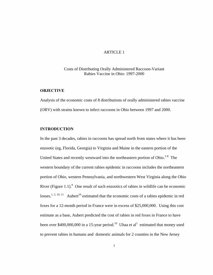
OBJECTIVE
Analysis of the economic costs of 8 distributions of orally administered rabies vaccine
(ORV) with strains known to infect raccoons in Ohio between 1997 and 2000.
INTRODUCTION
In the past 3 decades, rabies in raccoons has spread north from states where it has been
enzootic (eg, Florida, Georgia) to Virginia and Maine in the eastern portion of the
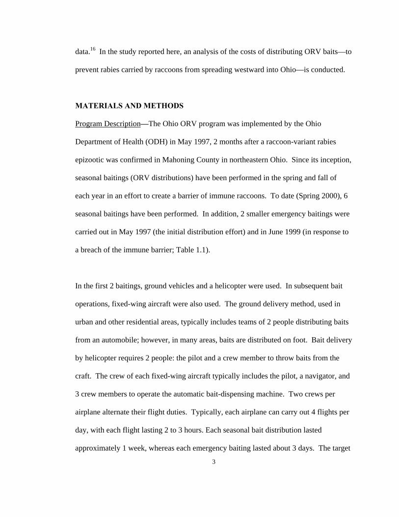
United States and recently westward into the northeastern portion of Ohio.1-8 The
western boundary of the current rabies epidemic in raccoons includes the northeastern
portion of Ohio, western Pennsylvania, and northwestern West Virginia along the Ohio
River (Figure 1.1).9 One result of such enzootics of rabies in wildlife can be economic
losses.1, 2, 10, 11 Aubert10 estimated that the economic costs of a rabies epidemic in red
foxes for a 12-month period in France were in excess of $25,000,000. Using this cost
estimate as a base, Aubert predicted the cost of rabies in red foxes in France to have
been over $400,000,000 in a 15-year period.10 Uhaa et al1 estimated that money used
to prevent rabies in humans and domestic animals for 2 counties in the New Jersey
2
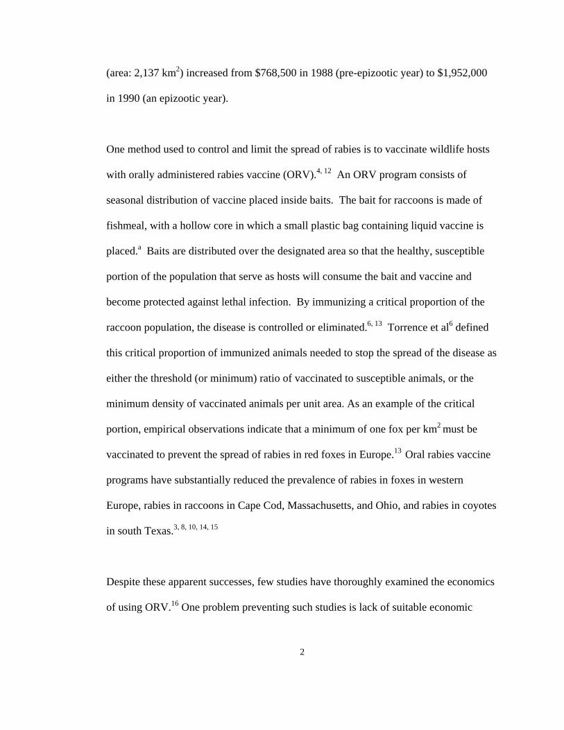
(area: 2,137 km2) increased from $768,500 in 1988 (pre-epizootic year) to $1,952,000
in 1990 (an epizootic year).
One method used to control and limit the spread of rabies is to vaccinate wildlife hosts
with orally administered rabies vaccine (ORV).4, 12 An ORV program consists of
seasonal distribution of vaccine placed inside baits. The bait for raccoons is made of
fishmeal, with a hollow core in which a small plastic bag containing liquid vaccine is
placed.a Baits are distributed over the designated area so that the healthy, susceptible
portion of the population that serve as hosts will consume the bait and vaccine and
become protected against lethal infection. By immunizing a critical proportion of the
raccoon population, the disease is controlled or eliminated.6, 13 Torrence et al6 defined
this critical proportion of immunized animals needed to stop the spread of the disease as
either the threshold (or minimum) ratio of vaccinated to susceptible animals, or the
minimum density of vaccinated animals per unit area. As an example of the critical
portion, empirical observations indicate that a minimum of one fox per km2 must be
vaccinated to prevent the spread of rabies in red foxes in Europe.13 Oral rabies vaccine
programs have substantially reduced the prevalence of rabies in foxes in western
Europe, rabies in raccoons in Cape Cod, Massachusetts, and Ohio, and rabies in coyotes
in south Texas.3, 8, 10, 14, 15
Despite these apparent successes, few studies have thoroughly examined the economics
of using ORV.16 One problem preventing such studies is lack of suitable economic
3
data.16 In the study reported here, an analysis of the costs of distributing ORV baits—to
prevent rabies carried by raccoons from spreading westward into Ohio—is conducted.
MATERIALS AND METHODS
Program Description—The Ohio ORV program was implemented by the Ohio
Department of Health (ODH) in May 1997, 2 months after a raccoon-variant rabies
epizootic was confirmed in Mahoning County in northeastern Ohio. Since its inception,
seasonal baitings (ORV distributions) have been performed in the spring and fall of
each year in an effort to create a barrier of immune raccoons. To date (Spring 2000), 6
seasonal baitings have been performed. In addition, 2 smaller emergency baitings were
carried out in May 1997 (the initial distribution effort) and in June 1999 (in response to
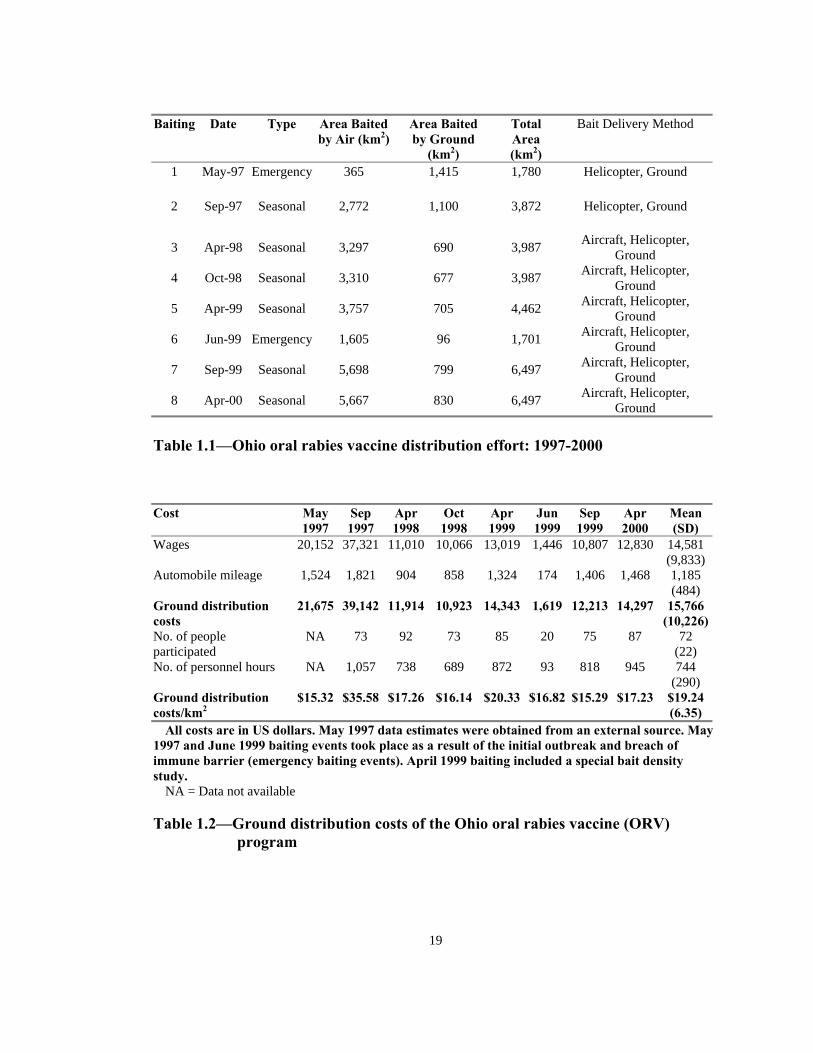
a breach of the immune barrier; Table 1.1).
In the first 2 baitings, ground vehicles and a helicopter were used. In subsequent bait
operations, fixed-wing aircraft were also used. The ground delivery method, used in
urban and other residential areas, typically includes teams of 2 people distributing baits
from an automobile; however, in many areas, baits are distributed on foot. Bait delivery
by helicopter requires 2 people: the pilot and a crew member to throw baits from the
craft. The crew of each fixed-wing aircraft typically includes the pilot, a navigator, and
3 crew members to operate the automatic bait-dispensing machine. Two crews per
airplane alternate their flight duties. Typically, each airplane can carry out 4 flights per
day, with each flight lasting 2 to 3 hours. Each seasonal bait distribution lasted
approximately 1 week, whereas each emergency baiting lasted about 3 days. The target
4
bait density for all methods of distribution was set at 75 baits/km2, with the exception of
the April 1999 baiting, when a bait density study was performed (Table 1.1).
Cost Data—Distribution cost data from each of the 8 baitings carried out from May
1997 to April 2000 were obtained (and, in some instances, estimated) by interviews,
field observations, and data provided by agencies involved in bait distribution efforts.
Costs were categorized by method of distribution (ground or air) and calculated in
dollars per square kilometer covered. In some instances, the areas baited with the use of
fixed-wing aircraft and helicopter overlapped; hence, the aerial distribution cost could
not be divided between these 2 delivery methods.
Ground distribution costs included automobile cost, valued at $0.31/mile, and the cost
of personnel who participated in the ground baiting. The personnel cost was calculated
by using the total amount of time each person spent on baiting and other ORV-related
tasks (driving to and from baiting areas, doing agency paperwork, etc.) multiplied by his
or her hourly wages, plus benefits. The amount of time that each person spent during
the ORV effort and his/her hourly wage rate was obtained from interviews.
The air distribution costs included helicopter cost, cost of fixed-wing aircraft (collected
in dollars per hour of flight time, including maintenance and insurance), cost of flight
crews, fuel cost, cost of administrative and support personnel, and miscellaneous costs.
Helicopter services including the aircraft and its pilot and fuel were contracted from the
Ohio Department of Transportation at a lump-sum rate. The cost of administrative and
5
support personnel supplied by ODH and other state and local agencies was recorded
separately.
The USDA Wildlife Services (USDA-WS) procured fixed-wing aircraft services from
the Ontario Ministry of Natural Resources (OMNR) at a fixed contract price. The
contract included the use of twin-engine fixed-wingb aircraft, each fitted with an ORV
bait-delivery mechanism. Contract price for each fixed-wing aircraft included the
salaries of 2 pilots, 1 engineer, and 2 bait specialists. However, after discussion with
the USDA-WS personnel who arranged the contract, it was decided that the negotiated
contract price may include an indirect subsidy, in that the USDA-WS may not be
charged the full cost of the services provided. To capture the true economic cost, or
opportunity cost, of fixed-wing aircraft services, it was estimated by obtaining hourly
rental rates of aircraft similar to those used in the bait distribution. The hourly rate
charged to rent an aircraft, including operation and maintenance costs, was quoted at
$1000 (Canadian) per hour (an average of $0.684 US per $1 Canadian was used for
calculation) by a private contractor.c Personnel cost was calculated by multiplying the
total time each person spent on the ORV project or was compensated for (ie, overtime,
time off) by his or her hourly wage. The wages of the flight crew and other payments to
them such as car rentals, hotel costs, per diem, and compensation time, were estimated
or obtained by interviews and field observation.
The ODH paid for the fuel used in the aircraft and also provided personnel for
administration of and participation in the ORV program. Wages, travel costs (mileage,
6
hotel, and per diem), and compensation time for ODH personnel and other local, state,
and federal agency employees who participated in the aerial distribution effort were
included in the aerial distribution costs. Data for such costs were collected by
interviewing each person involved and by field observation. Miscellaneous costs were
also collected using the same methods and included equipment rental, purchases, and
incidental costs for each of the baiting events.
The cost of the ORV, delivered to the ODH in bait form, was not included in the
estimates of distribution costs because it represented a fixed cost for the program, but it
was included in the calculations for the total cost. The cost of ORV was obtained from
the ODH, and the vaccine was purchased directly from the producer.a The overall bait
density was targeted at no less than 75 baits/km2, although local area modifications
were made by field staff because of variations in raccoon habitats. During the April
1999 baiting, a 1-time study was performed to determine the efficacy of different bait
densities, with some areas having a density as high as 300 baits/km2. Such densities
would not be considered “typical” and it was reasoned that the costs of bait distribution
associated with the experiment would be considerably higher than nonexperimental
distributions. Therefore the data collected during the April 1999 distribution was
considered as having the potential to distort the statistical analysis of the cost data (ie,
the April 1999 data are potential outliers). This conclusion led to adding an additional
set of calculations to the data analysis.

7
Data analyses—For each of the 8 bait operations and for each type of distribution
(ground or air), cost and input data were distributed into categories representing the
most important cost components (ie, wages, automobile mileage, helicopter fees).
Costs were then added and divided by the total area covered to provide a mean cost per
km2 for each bait operation. Means and SD were then calculated for the 8 bait
operations. Further, because the first seasonal operation (September 1997) and the
April 1999 operation (Table 1.1) may both be described as atypical, the means and SD
were recalculated, excluding the data from those operations. All data are reported as
mean ± SD.
RESULTS
Ground distribution costs—For ground distribution, 72 (± 22) people were used,
representing 744 (± 290) total personnel hours (Table 1.2). The September 1997
distribution had the highest mean costs because that operation used the most personnel
hours used for ground distribution. Personnel costs for the September 1997 distribution
accounted for approximately 30% of all ground distribution costs ($19.24/km2 ±
$6.35/km2). When the September 1997 and April 1999 data were removed (because
they were atypical), the cost for ground distribution was $16.34/km2 (± $0.82/km2).
Air distribution costs—Air distribution required 32 (±14) people, representing a mean
of 1,310 hours (± 476; Table 1.3). The data analyzed include the personnel flying and
staffing the helicopter and fixed-wing aircraft, who were paid under contracts. The
largest single cost was for the fixed-wing aircraft, at $40,248 (± $17,560) per baiting,
8
which accounted for approximately 37% of the total costs, or $24.71/km2 (±
$4.65/km2). When the September 1997 and April 1999 data were removed (atypical),
the cost for air distribution was $22.47/km2 (± $2.93/km2).
Total distribution costs—The total distribution costs ranged from $17.17/km2 (May
1997) to a maximum of $32.11/km2 (September 1997), with a mean of $23.23/km2 (±
$5.20/km2; Table 1.3). When the September 1997 and April 1999 data were removed
(atypical), the cost for total distribution was $20.58/km2 (± $2.78/km2). Most of the
costs were for aerial distribution (mean, $81,025; Table 1.3), which were 5.1 times
greater than ground distribution costs (mean, $15,766; Table 1.2).
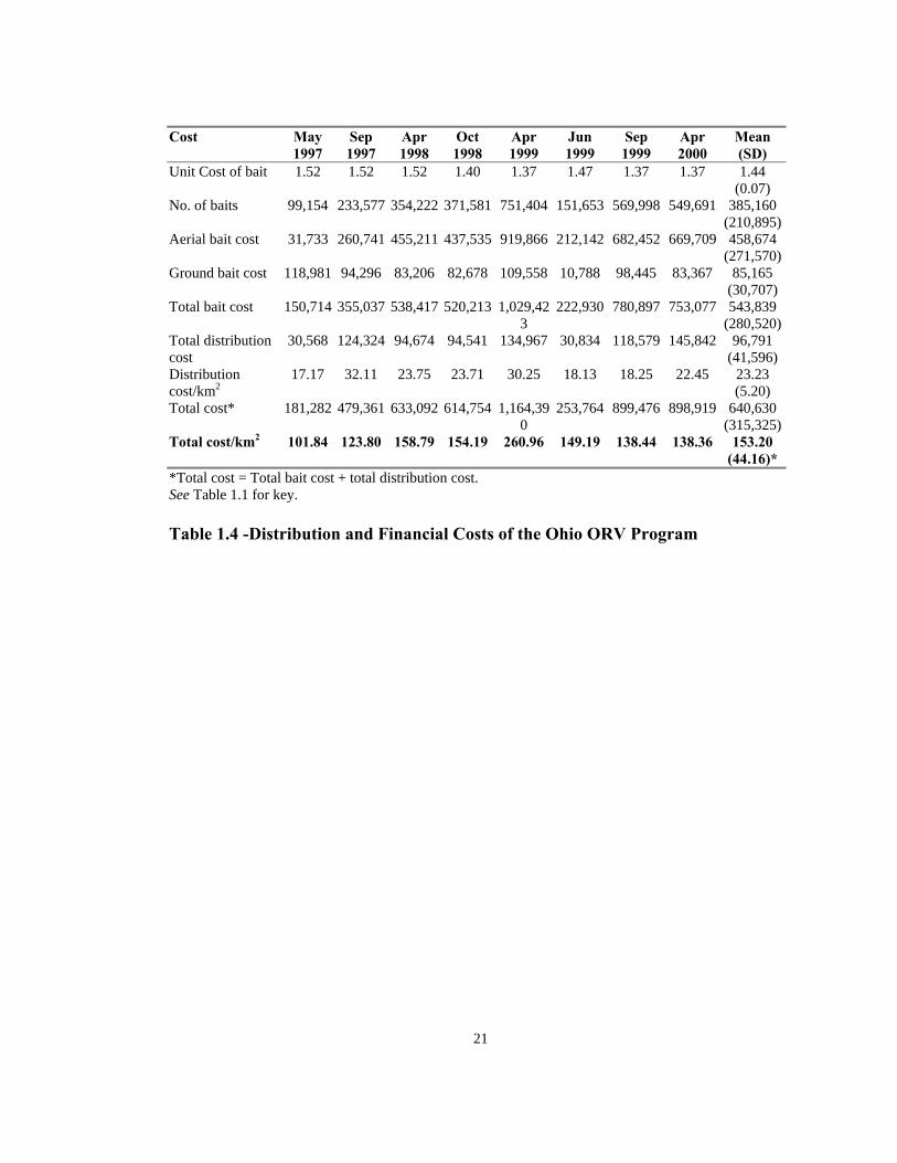
The number of baits distributed ranged from 99,154 in May 1997 to a maximum of
751,404 in April 1999 (Table 1.4). When the cost of these baits was added to
distribution costs, the total cost for a single bait operation was $153.20/km2 (±
$44.16/km2). The cost of the bait accounted for a mean of 85% of the total financial
cost per km2 baited.
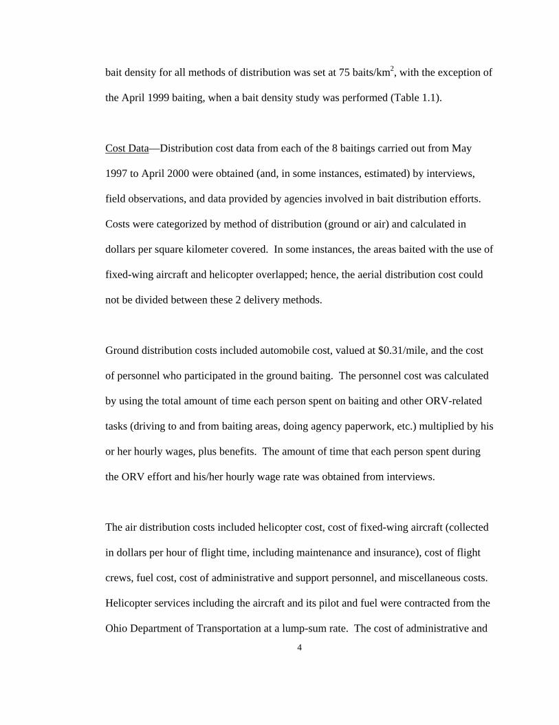
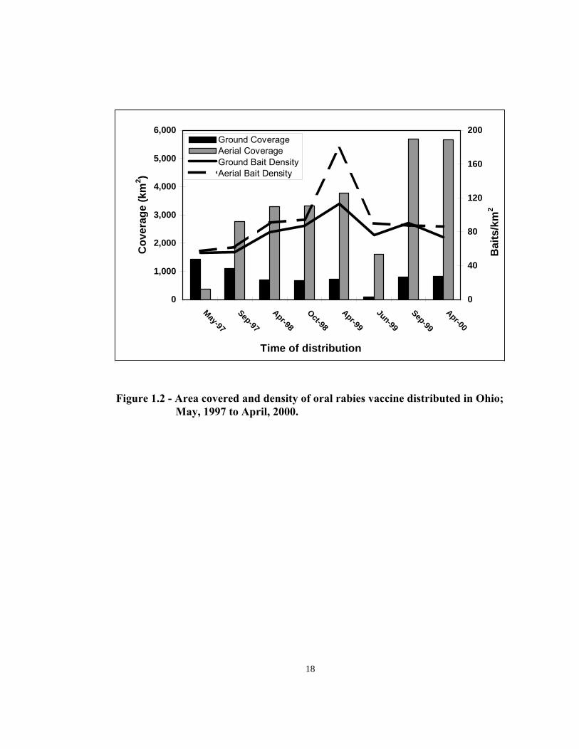
Area baited and bait densities—The area designated for seasonal ORV baiting had
increased from 3,872 km2 in September 1997 (1,100 km2 by ground; 2,772 km2 by air)
to 6,497 km2 in April 2000 (830 km2 by ground; 5,667 km2 by air; Figure 1.2). The
expansion in area covered was achieved with a major change in the way bait was
distributed. In May 1997, 79% of the area covered was done by the hand baiting
method but in April 2000, 87% of the area baited was done from the air. It was not
9
possible to subdivide the area baited from the air into areas baited exclusively by
helicopter and those baited exclusively by fixed-wing aircraft, because in some areas, to
ensure a higher density of baits, helicopters covered the same ground (ie, increased the
bait density) covered by fixed-wing aircraft.
A bait density of 91.00/km2 (± 32.10/km2) was achieved, with higher bait densities by
aerial distribution (Figure 1.2). When the April 1999 data were removed (atypical), the
bait density was 79.94/km2 (± 14.11/km2)
DISCUSSION
The ORV program for wildlife is the first immunologic tool to fight rabies in animal
hosts since vaccination of dogs became widely available in the 1940s. Although
successful application of ORV for rabies in foxes in Europe is well recognized, its use
for rabies in raccoons in the United States is still emerging.1, 3, 4, 10, 14 The lack of data
regarding the long-term effectiveness of the orally administered rabies vaccine used in
situations such as those described here prevents one from comparing the cost of various
distribution methods to the reduction of rabies (ie, performing a cost-effectiveness
analysis of the various distribution methods).
These distribution costs can be used to perform an economic cost-benefit analysis of an
ORV program.1, 2, 16, 17 In addition, the distribution costs can help determine the most
efficient means of distributing ORV in the future.
10
Uhaa et al1 provided an estimate of $100/km2/year for the “distribution systems costs,”
which they assumed include baiting by helicopter, fixed-wing aircraft and ground
(similar to this study). They did not, however, describe how they arrived at such a
figure. Moreover, in their sensitivity analyses, they did not alter this cost estimate even
though they varied bait density. This implies that they assumed that the distribution
cost is fixed. In this study, the mean cost of distribution in the Ohio ORV program is
$23.23/km2 (± SD, $5.20/km2/distribution), well below the assumed value in the
aforementioned study.1 Results of this study also revealed that a number of factors,
including differing bait densities, may cause the cost of distribution to change notably
(Tables 1.1-1.3). Aubert10 provided the only other specific estimate for the cost of
distribution: $9/km2 (bait delivery by helicopter of $7/km2; surveillance systems cost of
$2/km2) for distributing ORV to control rabies in red foxes in Europe. Unfortunately,
that report did not contain an explanation of how the estimate was obtained.
Furthermore, because the density of red foxes appears to be much lower than raccoons,
the density of ORV needed to control rabies in red foxes is probably much lower than
that needed to control rabies in raccoons.1, 10, 13, 14 And because these results
demonstrated that differences in densities of ORV impact costs of distribution, these
data cannot be directly compared with Aubert’s estimate. Therefore these results can be
considered to be the first explicit attempt to document the actual costs of distributing
ORV to control rabies in raccoons.
The data collected from 8 baiting operations revealed that although the costs of
distribution approximated only 15% of the total costs, they may vary considerably
11
(Table 1.4). For example, the September 1997 baiting had the highest distribution cost
of $32.11/km2, whereas distribution costs in May 1997, June 1999, and September 1999
were less than $20/km2. The high cost in September 1997 may be attributed to the fact
that it was the first large-scale ORV operation undertaken (double the area covered in
May 1997; Figure 1.2) by the agencies involved, and certain inefficiencies in a start-up
operation are expected. In addition, the entire air operation (2,772 km2) was performed
by helicopter and proved to be costly at $30.73/km2 (Table 1.3).
Even the ground baiting in the September 1997 operation, although it covered a smaller
area than the May 1997 ground baiting (Figure 1.2), was much more costly per square
kilometer ($35.58/km2) than the May 1997 baiting ($15.32/km2). This finding may be
attributable to the fact that the September 1997 baiting was more labor-intensive. A
more highly populated area (Youngstown, Ohio, and suburbs) was baited in September
1997, compared with the area baited in May 1997, which focused on the main roads
outside of Youngstown. Another potentially atypical baiting operation was performed
in April 1999, when several variations in strategies were tested, then adopted or
abandoned. Consequently, the April 1999 mean aerial baiting density (179 baits/km2)
and ground baiting density (113 baits/km2) were much higher than the remaining baiting
events (means: 81 baits/km2 for air, 74 baits/km2 for ground). This increased the total
cost per square kilometer by more than $100/km2 to $261/km2 (Table 1.4).
The increase in area baited increased total costs and was attributable to cases of rabid
raccoons within the immune barrier and breach of the immune barrier in June 1999.
12
Despite the higher distribution cost of aerial bait delivery, this method is indispensable
in areas with large tracts of farmland and forests where ground support is limited or
potential raccoon habitats are not easily accessible. In addition, to be fully effective,
baits must be distributed in a timely manner at critical periods of the year to
accommodate behavior of the raccoon population (ie, mating, foraging). Thus, despite
the expense, bait distribution by use of fixed-wing aircraft will continue to be the most
commonly used method of ORV distribution in Ohio.
Some economy of scale can be achieved by buying large quantities of baits. For
example, the reduction of bait cost by $0.15/unit ($1.52 in May 1997 to $1.37 in April
1999) resulted in savings of $112,710 for the 751,404 baits purchased in April 1999.
The net result is that the total cost of the Ohio ORV project seems to have stabilized at
approximately $140/km2 (September 1999, April 2000; Table 1.4).
Distribution costs may be further decreased as an optimal bait density strategy is
achieved. However, reduction in the amount of baits used per unit area will not affect
distribution costs with the same magnitude as it affects the total costs. For example,
increasing or decreasing aerial bait density will not substantially increase or decrease
the amount of personnel, personnel hours, equipment, or material required to distribute
bait.
Although changes in bait density may not have notably impacted distribution costs, it
appeared that, as the strategy matured, more consistent distribution costs were evident,
13
in the range of $18-$22/km2. Changes in distribution costs over time indicated that
there was a “learning curve” for establishment of an ORV program and many local,
state, and federal agencies and organizations need to collaborate. Cost estimates for the
last 2 baitings (September 1999 and April 2000) are perhaps more representative of an
established ORV program than earlier operations. The costs incurred in earlier
operations, however, serve as a reminder to other agencies in other locales
contemplating similar programs of the need to learn and improve upon delivery systems
as a program progresses through time.
Rabies in wildlife is typically a regional and persistent health problem; therefore, the
economic costs and benefits of an ORV program should be considered over a broad
region and over a long period. Collaboration among different regions could result in
several economies of scale, such as reduced price of ORV from purchasing large
quantities of baits. Regional cooperation could also lead to economies of scale by
hiring new personnel and purchasing new equipment and material, both of which are
currently being contracted out to external agencies (eg, fixed-wing aircraft, pilots, etc.).
The information presented here can be combined with knowledge on raccoon ecology
and epidemiologic characteristic of rabies in raccoons to predict future spread of rabies
as well as the economic impact of using ORV. Several scenarios may need to be
evaluated, and they will be important in determining the feasibility of regional and
national efforts and in designing future interventions to control this public health
problem.

14
a Raboral (Rhone Merieux), Merial Inc., Athens, Georgia.
b De Havilland Corporation, Taylor, Michigan.
c Rudy Kellar, First Air, Ottawa, Ontario, personal communication, May 1998.
15
REFERENCES: ARTICLE 1
1. Uhaa LJ, Dato VM, Sorhage FE, et al. Benefits and costs of using an orally
absorbed vaccine to control rabies in raccoons. J Am Vet Med Assoc 1992;
201:1873-1882.
2. Kreindel SM, McGuill M, Meltzer M, et al. The cost of rabies postexposure
prophylaxis: One state’s experience. Public Health Rep 1998; 13:247-251.
3. Robbins AH, Borden MD, Windmiller BS, et al. Prevention of the spread of rabies
to wildlife by oral rabies vaccination of raccoons in Massachusetts. J Am Vet Med
Assoc 1998; 213:1407-1412.
4. Winkler WG, Jenkins SR. Raccoon rabies. In: Baer GM, ed. The natural history of
rabies. 2nd ed. Boca Raton, FL: CRC Press Inc.; 1991:325-340.
5. Fischman HR, Grigor JK, Horman JT, et al. Epizootic of rabies in raccoons in
Maryland from 1981 to 1987. J Am Vet Med Assoc 1992; 201:1883-1886.
6. Torrence ME, Jenkins SR, Glickman LT. Epidemology of raccoon rabies in
Virginia, 1984 to 1989. J Wildl Dis 1992; 28:369-376.
7. Krebs JW, Rupprecht CE, Childs JE. Rabies surveillance in the United States
during 1999. J Am Vet Med Assoc 2000; 217:1799-1811.
8. Smith KA. Update on rabies in Ohio. Ohio Vet Med Assoc Newslett 1998; 29:5.
9. Wandeler A, Rosatte RC, Williams D, et al. Update: Raccoon rabies epizootic -
United States and Canada, 1999. MMWR Morb Mortal Wkly Rep 2000; 49:31-35.
10. Aubert, MFA. Costs and benefits of rabies control in wildlife in France. Rev sci
tech 1999; 18:533-543.
16
11. Nelson RS, Cooper GH, Cartter ML, et al. Rabies postexposure prohylaxis—
Connecticut, 1990-1994. MMWR Morb Mortal Wkly Rep 1996; 45:232-234.
12. Rupprecht CE, Wiktor TJ, Johnston DH, et al. Oral immunization and protection of
raccoons (Procyon lotor) with a vaccinia-rabies glycoprotein recombinant virus
vaccine. Proc Natl Acad Sci U S A 1986; 83:7947-7950.
13. Anderson RM, Jackson HC, May RM, et al. Population dynamics of fox rabies in
Europe. Nature 1981; 289:765-771.
14. Wandeler AI. Oral immunization of wildlife. In: Baer GM, ed. The natural history
of rabies. 2nd ed. Boca Raton, FL: CRC Press Inc., 1991; 485-503.
15. Fearneyhough MG, Wilson PJ, Clark KA, et al. Results of an oral rabies
vaccination program for coyotes. J Am Vet Med Assoc 1998; 212:498-502.
16. Meltzer MI, Rupprecht CE. A review of the economics of the prevention and
control of rabies,” Pharmacoeconomics 1998; 14:365-383.
17. Meltzer, MI. Assessing the costs and benefits of an oral vaccine for raccoon rabies:
a possible model. Emerg Infect Dis 1996; 2:336-342.

Figure 1.1—Detection of rabies in raccoons (by year) in the United States and Canada9
17
0
1,000
2,000
3,000
4,000
5,000
6,000
May-97
Sep-97
Apr-98
Oct-98
Apr-99
Jun-99
Sep-99
Apr-00
Cov
erag
e (k
m2 )
0
40
80
120
160
200
Bai
ts/k
m2
Ground CoverageAerial CoverageGround Bait DensityAerial Bait Density
Time of distribution
Figure 1.2 - Area covered and density of oral rabies vaccine distributed in Ohio; May, 1997 to April, 2000.
18
19
Baiting Date Type Area Baited
by Air (km2)Area Baited by Ground
(km2)
Total Area (km2)
Bait Delivery Method
1 May-97 Emergency 365 1,415 1,780 Helicopter, Ground
2 Sep-97 Seasonal 2,772 1,100 3,872 Helicopter, Ground
3 Apr-98 Seasonal 3,297 690 3,987 Aircraft, Helicopter, Ground
4 Oct-98 Seasonal 3,310 677 3,987 Aircraft, Helicopter, Ground
5 Apr-99 Seasonal 3,757 705 4,462 Aircraft, Helicopter, Ground
6 Jun-99 Emergency 1,605 96 1,701 Aircraft, Helicopter, Ground
7 Sep-99 Seasonal 5,698 799 6,497 Aircraft, Helicopter, Ground
8 Apr-00 Seasonal 5,667 830 6,497 Aircraft, Helicopter, Ground
Table 1.1—Ohio oral rabies vaccine distribution effort: 1997-2000 Cost May
1997 Sep 1997
Apr 1998
Oct 1998
Apr 1999
Jun 1999
Sep 1999
Apr 2000
Mean (SD)
Wages 20,152 37,321 11,010 10,066 13,019 1,446 10,807 12,830 14,581 (9,833)
Automobile mileage 1,524 1,821 904 858 1,324 174 1,406 1,468 1,185 (484)
Ground distribution costs
21,675 39,142 11,914 10,923 14,343 1,619 12,213 14,297 15,766 (10,226)
No. of people participated
NA 73 92 73 85 20 75 87 72 (22)
No. of personnel hours NA 1,057 738 689 872 93 818 945 744 (290)
Ground distribution costs/km2
$15.32 $35.58 $17.26 $16.14 $20.33 $16.82 $15.29 $17.23 $19.24 (6.35)
All costs are in US dollars. May 1997 data estimates were obtained from an external source. May 1997 and June 1999 baiting events took place as a result of the initial outbreak and breach of immune barrier (emergency baiting events). April 1999 baiting included a special bait density study. NA = Data not available Table 1.2—Ground distribution costs of the Ohio oral rabies vaccine (ORV)
program

20
Cost May
1997 Sep 1997
Apr 1998
Oct 1998
Apr 1999
Jun 1999
Sep 1999
Apr 2000
Mean (SD)
Helicopter (incl. fuel, pilot)
6,392 60,606 8,495 2,385 5,744 3,277 2,500 13,265 12,833 (18,372)
Administrative and support crew
2,500 21,472 31,487 32,338 28,423 5,019 28,250 34,682 23,021 (11,718)
Aircraft personnel (OMNR) cost
N/A N/A 9,685 10,394 16,134 3,454 11,880 16,308 11,309 (4,355)
Aircraft running cost
N/A N/A 27,648 29,660 59,983 13,404 53,152 57,641 40,248 (17,559)
Aircraft fuel cost N/A N/A 5,445 7,574 9,641 3,149 8,890 9,292 7,332 (2,335)
Other costs N/A 3,104 0 1,265 699 912 1,695 357 1,147 (952)
Total air distribution costs
8,892 85,182 82,761 83,617 120,624 29,215 106,366 131,545 81,025 (39,807)
No. of people participated
NA 10 25 41 41 14 48 45 32 (14)
No. of personnel hours
NA 908 1357 1416 1852 364 1557 1714 1,310 (476)
Air distribution costs/km2
24.36 30.73 25.10 25.26 32.11 18.21 18.67 23.21 24.71 (4.65)
OMNR = Ontario Ministry of Natural Resources, N/A = Not applicable. See Table 1.1 for key. Table 1.3—Air Distribution Costs of the Ohio ORV Program
21
Cost May
1997 Sep 1997
Apr 1998
Oct 1998
Apr 1999
Jun 1999
Sep 1999
Apr 2000
Mean (SD)
Unit Cost of bait 1.52 1.52 1.52 1.40 1.37 1.47 1.37 1.37 1.44 (0.07)
No. of baits 99,154 233,577 354,222 371,581 751,404 151,653 569,998 549,691 385,160 (210,895)
Aerial bait cost 31,733 260,741 455,211 437,535 919,866 212,142 682,452 669,709 458,674 (271,570)
Ground bait cost 118,981 94,296 83,206 82,678 109,558 10,788 98,445 83,367 85,165 (30,707)
Total bait cost 150,714 355,037 538,417 520,213 1,029,423
222,930 780,897 753,077 543,839 (280,520)
Total distribution cost
30,568 124,324 94,674 94,541 134,967 30,834 118,579 145,842 96,791 (41,596)
Distribution cost/km2
17.17 32.11 23.75 23.71 30.25 18.13 18.25 22.45 23.23 (5.20)
Total cost* 181,282 479,361 633,092 614,754 1,164,390
253,764 899,476 898,919 640,630 (315,325)
Total cost/km2 101.84 123.80 158.79 154.19 260.96 149.19 138.44 138.36 153.20 (44.16)*
*Total cost = Total bait cost + total distribution cost. See Table 1.1 for key. Table 1.4 -Distribution and Financial Costs of the Ohio ORV Program
22
ARTICLE 2
Predicting Movement of an Infectious Disease: An Agent-Based Modeling Approach
OBJECTIVE
To implement agent-based modeling as an approach to predict movement of raccoon
rabies across time and space.
INTRODUCTION
Prediction of movement of infectious disease across time and space can be an important
tool for the basis of provision of funds and efficient use of resources available to the
public health policy maker. Movement of disease has traditionally been modeled in the
mathematics arena, typically through a system of ordinary differential equations.1-4
These models use characteristics of highly aggregated groups of agents (e.g.,
susceptible or infected) to simulate the dynamics of the ecology and the epidemic
process of the entire population. Extensions of these population-based models (PBMs)
have distinguished fragments of the population by such characteristics and behaviors as
gender, age, degree of dispersal, and mortality rate; however, none of these models have
been inclusive of all these realisms.5-8 In contrast, some PBMs ignore the host-
23
pathogen relationship and indirectly predict the advance of an epidemic by utilizing the
heterogeneity of geographical areas as explanatory varibales.9, 10
In agent-based modeling (ABM) the population is treated as a collection of
heterogeneous agents who autonomously make decisions, interact with their
environment and each other, and ultimately give rise to macro phenomena. In ABM,
agents are assigned a wide variety of characteristics drawn from realistic distributions of
such attributes. Agent behavior also can be shaped by characteristics of the
geographical areas to which agents are assigned. With recent advances in computer
technology, available computational power allows physical and social scientists to
model a large number of heterogeneous agents with complex behavior acting on a
heterogeneous landscape.11 In addition, characterizing the model’s spatial units with
real-world data from a geographic information system (GIS) database can greatly
enhance the applicability of ABM models.12
In this paper, a hypothetical raccoon rabies epidemic is simulated within an ABM
framework. The landscape in which the raccoon agents operate is divided into spatial
units characterized by land use (see Model, below). In the style of Epstein and Axtell’s
“SugarScape” model, the raccoon agents are characterized by their gender, genotype
(home range and metabolism), fat reserve (accumulated nutrient), and health
(susceptiblity) (see Model).13 These raccoon agents migrate in and out of the model’s
space, search for nutrients, reproduce, transmit disease, and ultimately cause economic
consequences. The rabies incidences in each simulation map out the economic damages
24
that the disease causes based on whether the disease is in its epidemic or endemic stage
(see Models below).
METHODS
In addition to the Java programs which constitute the model (see Model, below), other
public-use software programs are used that include model management activities such
as scheduling, control of time, data collection, “garbage collection” (removal of
unnecessary data from computer’s memory), and visuals. The management activities
are supported by a library of Java programs packaged in an interface called RePast
provided by the Social Science Computing Research Center of the University of
Chicago (version 2.0; distributed at http://repast.sourceforge.net/). The programs are
compiled on an IBM personal computer with a Java compiler (Java 2 Platform,
Standard Edition, version 1.4.2; distributed at
http://java.sun.com/j2se/1.4.2/download.html). The results of the model are used to
verify if they conform with cited literature relating to raccoon ecology. Two different
epidemic regimes (aggressive and non-aggressive) are simulated and compared (see
Epidemic rule, below). The results of the simulations are compared in regards to the
rate of movement of the epidemic front, and the relative intensity of raccoon rabies by
geographical area.
MODELS
The models consist of a set of Java programs that specify the assignment of
characteristics, and algorithms that describe the behaviors for each spatial unit {Ē} and
25
raccoon agent {Ā}. The set of characteristics and behaviors ({Ē}, {Ā}), described in
detail below, is based on abstract constructs and ecological and epidemiological
parameters from available literature (see Appendix). The set ({Ē}, {Ā}) represents an
artificial landscape where synthetic raccoon agents roam through time. The
environmental characteristics in this model, EC (explained below), include the
resolution of the space and the nutrient ranking of spatial units by land category. The
environmental behavior consists of a nutrient grow back algorithm, G. Therefore,
environmental characteristics and behavior can compactly be noted as Ē = {EC; G}.
Raccoon agent characteristics (AC) include gender, current age, death age, fat reserve,
home range, and metabolism. Raccoon agent behavior includes movement (M),
migration (Mi), reproduction (R), and epidemic transmission (E). The cost of raccoon
rabies (C) encapsulates the set of behaviors of the raccoon agent. Therefore, the set of
characteristics and behaviors which describe a raccoon agent is represented by Ā =
{AC; M, Mi, R, E, C). Each time period in a simulation represents 1 week. Each
simulation run consists of 2600 periods, which represents 50 years (each year is
approximated to 52 weeks). Due to time constraint, only one run for each model is
simulated with the exception of comparison of pre-epidemic population densities where
two independent runs with the same specifications were compared.
Environmental characteristics, EC
Resolution and nutrient capacity
Resolution and type of environment serve as important variables in determination of
raccoon population density (see Figure 2.1). The environment is comprised of a lattice
26
of two-dimensional square cells where each cell represents an area of 100 m2 allowing a
maximum density of 100 raccoons per km2. Barring extreme population densities
usually found in southern swamps,14, 15 there is a general consensus on the order of
desirable habitat for the raccoon population (see Table 2.1). Raccoon densities of
approximately 70/km2 in a suburban area in Ohio, up to 50/km2 in areas adjacent to
bodies of water (marshes, swamps, and bottomlands) in eastern US, and up to 20/km2 in
farmlands in the eastern US have been reported.15 There have also been reports of
approximately 15 raccoons/km2 in a hollow in Virginia, and up to 5 raccoons/km2 in
prairies in North Dakota and Manitoba.15, 16
Table 2.1 shows the ranking of categories of land use—based on reported upper limit
values—in descending order where a higher ranking indirectly indicates more available
nutrient for the raccoon agent. Hence, these rankings can serve as the nutrient capacity
for the corresponding land use.
Environmental behavior
As a result of the raccoon agent’s movement behavior (see Movement rule, below), the
nutrient levels of occupied spaces fall below their capacity. The process of nutrient
generation for different spatial units back to their capacity is not known and may be a
complex function of other processes. Two different nutrient grow back (regeneration)
rules are used to assess the sensitivity of the models to the environmental behavior.
Differentiating the nutrient grow back algorithm allows us to test whether changing the
algorithm from the Simple format to the Urban (see below) leads to different spatial
27
patterns and/or higher population densities. There is a myriad of other land use
designation and nutrient grow back algorithms that could otherwise be used. For
example, farmland may have different seasonal grow back rates or wetlands can have a
relatively higher grow back rates. One may also use cardinal measures of nutrient
availability for each land use.
Simple grow back rule, G1
It is assumed that the value of nutrient for each spatial unit is increased at 1 unit per
period up to its capacity level.
Urban grow back rule, G1, G∞
It is postulated that in urban and suburban areas, where human garbage serves as the
primary food source for raccoons, the nutrient source for raccoons is replenished
weekly up to its capacity. For other areas, it is assumed that the value of nutrient is
increased at 1 unit per period up to its capacity level.
Agent characteristics, AC
Kaufmann (1982) presents the most detailed description of the age distribution of
raccoon population (see Appendix). He reports that although a raccoon can live in the
wild for up to 16 years, most die within the first two years and only 1/100 live up to the
age of 7 years.15 Major factors of morbidity are harsh weather for juveniles, road kills,
hunting, and trapping.17 For example, in 1981 an estimated 846,000 raccoons were
killed in Pennsylvania as a result of hunting activities.17 Assuming a 5% newborn
28
mortality, mortality rate of 60% of raccoons of up to a year old, 75% total mortality of a
generation of raccoons within their first 2 years, and that 1/1000 raccoon reaches the
age of 16, a hypothetical age distribution and its associated probabilities can be
constructed for the raccoon population (see Figure 2.2 and Appendix).
When introduced to the simulation, each raccoon agent is randomly assigned a gender
and a maximum age, and randomly drawn from the probability distribution described in
Figure 2.2. In addition, first generation raccoons are randomly assigned a location in
the environment, a proxy fat reserve (nutrient endowment) value drawn from a uniform
distribution (minimum: 5, maximum 50) (U(5, 50)), and a proxy genotype: a home
range level U(1, 7) and a metabolism level U(1, 5). Fat reserve, metabolism, and
agent’s successful movement in attaining more nutrients (see Movement rule, below)
represent the competition the raccoon agents pose toward each other in search of
nutrients. As a result, a morbidity factor of starvation may further reduce the maximum
age of some raccoon agents.
Home range of a raccoon consists of the geographic area that it normally scouts for
food. Merritt17 estimates a range of 0.05-50 km2/year for raccoons in Pennsylvania
while Kaufmann15 reports typical estimates of 0.4-1 km2 and up to 7.07 km2 on a daily
basis (also see Appendix). In this model, an agent with a home range level of 14 can
have a weekly home range of up to 8.41 km2 (see Figure 2.4, and Environmental
characteristics, above). Although studies have been conducted on the extent of home
range for raccoons, the home range distribution is not well known. Therefore, for each
29
model uniform distribution (U(1, 14)) is used for agent’s home range, a counterpart
model with normal distribution with mean of 7.5 km2 and standard deviation of 2 km2
(N(7.5, 2)) is used to assess the sensitivity of models’ results to this variable (e.g.,
Model 1 uses uniform home range versus Model 3 which uses normal home range; see
Table 2.2). Figure 2.5 shows the cumulative distribution function of the normal and
uniform distributions. Genotypes of subsequent generations are assigned according to
their parents’ genotypes (see Reproduction rule, below). Agents are also characterized
by their health: susceptible, infected, or incubating (see Epidemic rule, below).
Agent Behavior
Movement rule, M
Each agent moves once per period within its home range. Movements by agents are
made sequentially and the order of movement by agents is randomly shuffled after
every period. The movement rule is comprised of two different algorithms: one for the
susceptible and incubating agents (MS,Inc) and the other for the infected agents who
move randomly (MInf).
Movement algorithm MS,Inc
Within its home range, an agent moves to an unoccupied space with the highest level of
nutrient and adds the amount of nutrient to its fat reserve. An amount equal to the
agent’s metabolism is then decreased from its fat reserve.
Movement algorithm MInf
30
The movement of infected agents is the same as above with the exception that the agent
moves randomly within its home range and afflicts susceptible agents within its path to
the new position and/or in the adjoining cells at its new position (see Algorithms EA and
EN, below).
Migration rule, Mi
To resolve the interaction of the space and agent objects of the contiguous land area
outside the model boundaries with those objects within the model’s space, a migration
rule is devised to facilitate migration of raccoon agents to and from the model’s space.
The raccoon agents are allowed to leave the boundary areas of the model’s space if the
population density within their home range exceeds a certain limit. Conversely, if the
population density of agents along the borders of the model’s space become sparse due
to disease transmission, other susceptible raccoon agents migrate into the model’s
space.
Migration algorithm
If the raccoon population density exceeds a certain limit (90/km2 used in models in this
study) within the home range of a raccoon agent, and its home range range extends
beyond the border of the model’s space, the raccoon agent leaves the model’s space. If
the raccoon population density is 0/km2 and the average nutrient value of the space is at
least 1 unit/km2 around the border of the model’s space, a susceptible raccoon agent
with a random maximum age drawn from the probability distribution in Figure 2.2,
metabolism (U(1, 5)), and home range (U(1, 14)) enters the model’s space.
31
Reproduction rule, R
In order to reproduce, it must be mating season and the agents must be fertile. The start
of the calendar year 0 is arbitrarily set to correspond with the week of August 21.
Raccoon mating season extends from January to March; although, raccoon mating has
been observed into the summer months.15-18, 20, 21 Two different mating season lengths
are used in the simulations: 13-week (early January to early April), and 21-week (early
January to early June). For example, Model 5 and Model 6 are differentiated only by
their mating season length. Typically, male raccoons do not mate until the end of their
second year while about 60% of female yearlings mate. 15, 18-20 Hence, in the model,
sixty percent of female yearlings are deemed fertile and male raccoon agents cannot
reproduce until their second year. Female agents can mate only once per mating season.
If there are no mates within home range of a fertile agent, the movement rule is
followed (see above).
Reproduction algorithm
Within its home range, an agent selects the nearest susceptible neighbor of the opposite
sex. If the neighbor is fertile and there is an adjacent empty space to the neighbor, the
agent occupies the empty space and adds the amount of nutrient of that site to its
strength. An amount equal to the agent’s metabolism is then decreased from its strength.
The female agent becomes pregnant. Raccoons have a gestation period of 60-73 days;15-
19, 21 hence, a gestation period of 9 or 10 weeks is determined randomly from a uniform
distribution. Raccoons have a litter of 1-7 offspring per birth, with a typical litter of

32
3-4.15-19, 21 Therefore, the number of offspring is determined randomly from a truncated
normal distribution (N(3.5, 1)). After the gestation period is over, the offspring and
their mother move together typically between 16 and 20 weeks and may live with the
mother up to one year before the arrival of the next litter.15-18, 19 To simulate this time
range, after a period of 18 weeks, half of the mothers wean their offspring, and the
young are “born” in the mother’s home range; the other half wean their offspring at 52
weeks. If there are not enough empty spaces within the mother’s home range, the
number of offspring is adjusted downward forcing the maximum limit of 100
raccoons/km2. The home range and metabolism are assigned to each offspring
randomly from a uniform distribution within the range of parents’ home range and
metabolism levels. For example, if the home range of parent 1 is 3 and home range of
parent 2 is 5, then home range of each offspring will be randomly drawn from a uniform
distribution with a minimum of 0.49 km2 and maximum of 1.21 km2 (U(3, 5)) (see
Figure 2.4 for further explanation).
Epidemic rule, E
Rabies incubation period in raccoons lasts 10-79 days; therefore, a newly infected agent
in the model incubates for 1-11 week(s) and avoids contact with other agents.22
Following the incubation period, the agent acquires a large home range and metabolism
and dies within 2 weeks of clinical disease.22 Infected agents cannot reproduce. Each
model was run twice using two different algorithms for the disease transmission
process: a “non-aggressive” regime (EN) and an “aggressive” regime (EA).
33
Epidemic algorithm EN
An infected agent moves randomly to an unoccupied space within its home range and
adds the amount of nutrient available at the new position to its fat reserve. An amount
equal to the agent’s metabolism is then decreased from its strength. The rabid agent
afflicts all of its susceptible neighbors (up to 8 agents) with rabies. The newly infected
agent(s) acquires high metabolism of 5 units, a large home range of 14 units (8.4 km2
home range), and then enters its incubation period (U(1, 8) weeks). After the
incubation period is over, the newly infected agent dies within U(1, 2) weeks.
Epidemic algorithm EA
In addition to EN, the agent also infects all susceptible agents within its shortest path to
the new location (up to 20 agents including susceptible neighbors at new location).
RESULTS
The model’s space, a hypothetical 20-kilometer square area, is comprised of a lattice of
100-m2 grids (total of 40,000 spatial units). The composition of the landscape is
designated as 20% urban, 20% wetland, 20% farmland, 15% forest, 15% prairie, 5%
water and 5% other (see also Environmental characteristics, above). Figure 2.3 shows a
spatial representation of the model’s space with darker colors representing more
nutritious spatial spaces. The model’s space is further divided into 16 quadrants (see
Figure 2.3) representing potential political divisions in a real life scenario. Initially
8,000 agents (20 agents/km2) are introduced to the space at period 0. At period 500,
and every two weeks thereafter, a rabid agent breaches the southern border of the

34
model’s space (quadrants 13-16, see Figure 2.3). Sixteen separate models differentiated
with the type of epidemic process, nutrient growback rule, home range distribution and
mating season length are simulated (see Table 2.2).
Pre-epidemic population densities
Table 2.3 presents the average population densities—based on one run for each
model—by land use category for the 16 models. The average total population densities
range from 8.76 (Model 1) to 14.57 raccoons/km2 (Model 16) (average = 11.44,
standard deviation = 1.74). Individually, the t-ratios of the average total population
densities for the 16 models, on the basis of a two-tail t test, are all significant at 1% (see
Table 2.3). In other words, total population densities for each quadrant did not
significantly change from one period to another for the length of the simulation (2600
periods). For models with Simple nutrient grow back regime (Models 1-4 & 9-12), the
average urban population densities range from 19.57 (Model 1) to 22.06 raccoons/km2
(Model 4) (ave. = 20.70, s.d. = 0.82) while urban population densities of models with
Urban nutrient grow back regime (Models 5-8 & 13-16) range from 47.67 (Model 5) to
63.07 raccoons/km2 (Model 16) (ave. = 56.34, s.d. = 5.33). Individually, the t-ratios for
all average urban population densities were significant at either 1% (5 cases) or 0.1%
(11 cases) (see Table 2.3).
Wetland population densities for models with Simple nutrient grow back algorithm
range from 16.15 (Model 1) to 21.03 raccoons/km2 (Model 4) (ave. = 18.54, s.d. =
1.59), while the models with Urban nutrient grow back range from 3.10 (Model 5) to
35
5.47 raccoons/km2 (Model 16) (ave. = 3.90, s.d. = 0.80). Individually, on a basis of a
two tail test, four models have a significant t-ratio at the 0.1% level, four models are
significant at 1%, and five models are significant at 20% (see Table 2.3). The
remaining three wetland population density estimates are statistically insignificant.
Farmland population densities range from 6.92 to 13.52 raccoon/km2 in models with
Simple nutrient grow back algorithm (ave. = 10.03, s.d. = 2.14), and range from 2.53 to
3.44 raccoons/km2 in Urban models (ave. = 2.86, s.d. = 0.28). The t-ratios of six of the
farmland population density estimates are significant at the 20% level, three are
significant at 10%, and the remaining nine estimates are statistically insignificant.
Population density estimates for land use classes of forest, prairie, other, and inhabitable
are all statistically insignificant. The lack of significance for these land uses may be
partly explained by random placement of initial generation of the agents, random
placement of migrants into the model, and congestion. Due to the insignificance of
results of these land uses, discussion on effects of nutrient grow back algorithm, home
range distribution, and length of mating season are focused on total, urban, wetland and
farmland density estimates.
Cross-effect of nutrient grow back algorithm
Nutrient capacity based on land use designation and nutrient grow back algorithm make
up the desirability of different spatial units to agents; hence, they are important factors
in shaping the spatial distribution of the agents in the model. Nutrient capacity is
designated with ordinal ranking of land use categories used in the model (see Table
2.1). Two different nutrient grow back algorithms are used in the model: Simple and
Urban (see Environmental behavior, above).
Tables 2.4 and 2.5 present average densities for total, urban, wetland, and farmland
populations. The remaining land uses are found to be statistically insignificant (see
above). Average values in Tables 2.4 and 2.5 are based on the average of density
estimates of each pair of identical models (before the onset of epidemic).
As expected, urban population density estimates of models with Urban nutrient grow
back algorithm, on average, are larger (272%) than models with Simple nutrient grow
back algorithm. On the other hand, population density estimates for wetland and
farmland areas in the Simple nutrient grow back algorithm, on average, are 4.8 and 3.5
times larger than their Urban nutrient grow back counterparts. Different null and
alternative hypotheses are considered for each group of population densities:
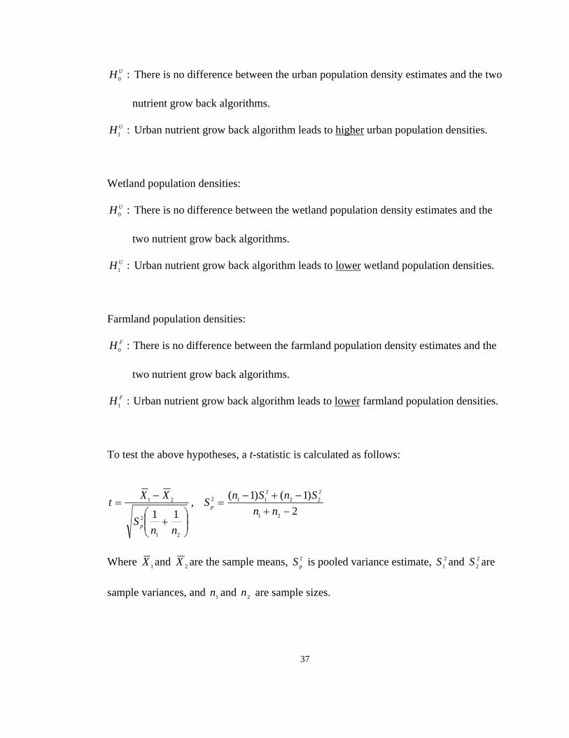
Total population densities:
36
o :0T There is no difference between the total population density estimates and the tw
nutrient grow back algorithms.
H
:1TH Urban nutrient grow back algorithm leads to higher total population densities.
Urban population densities:
:0UH
37
o
nutrient grow back algorithms.
algorithm leads to higher
There is no difference between the urban population density estimates and the tw
:1UH Urban nutrient grow back urban population densities.
Wetla
two nutrient grow back algorithms.
algorithm leads to lower
nd population densities:
:0UH There is no difference between the wetland population density estimates and the
:UH Urban nutrient grow back 1 wetland population densities.
Farmland population densities:
two nutrient grow back algorithms.
:0FH There is no difference between the farmland population density estimates and the
H :F Urban nutrient grow back algorithm leads to lower1 farmland population densities.
t-statistic is calculated as follows: To test the above hypotheses, a
⎟⎟⎠
⎞⎛= 21
11t ,
⎜⎜⎝
+
−
21
2
nnS
XX
p
22211
−+=
nnS )1()1(
21
222 −+− SnSnp
Where 1X and 2X are the sample means, 2
pS is pooled variance estimate, 21S and 2
2S a
sample variances, and n and n are sample sizes.
re
1 2
38
l
el of significance. The t statistics for
.
ter
indicates that either there is more of
chance meeting between fertile mates during mating season and/or there are fewer
The t-test results in Table 2.6 also indicate
f
Table 2.6 presents the calculated value for the t statistics for the above tests. For the
total population density estimates, the t statistic indicates that, on the basis of a one-tai
test, the null hypothesis is rejected at the 2.5% lev
the urban and wetland population density estimates indicate, on the basis of a one-tail
test, that their respective null hypotheses are rejected at the 0.05% level of significance
Lastly, null hypothesis for the farmland population density estimates, based on a one-
tail test, is rejected at 0.5% level of significance.
Overall, the Urban nutrient grow back algorithm causes the agents to intensively clus
in the urban areas and attract agents that otherwise would have stayed in the wetlands
and farmlands. The fact that the total population density estimate is also significantly
higher for the Urban nutrient grow back algorithm
a
deaths as caused by starvation of agents.
that the choice of nutrient grow back algorithm is significant regardless of the choice o
home range distribution or mating season length.
Cross-effect of home range distribution
A sensitivity analysis of the home range distribution of the agents is conducted to tes
whether the home range distribution significantly affects the models’ results. Simila
the analysis in Table 2.6, Table 2.7 presents a group of pair-wise comparisons between
models with uniform and normal distribution. For example, observation 1 consi
averages of Models 1 & 9 (uniform distribution) versus averages of Models 3 & 11
(normal distribution). Constructing null hypotheses in the same fashion as above
t
r to
ders the
39
ack algorithm. For this reason, a Z
test is conducted between individual samples which are only differentiated by the home
range distribution: Model 1 versus 3, Model 2 versus 4, Model 5 versus 7, Model 6
ersus 8, Model 9 versus 11, Model 10 versus 12, Model 13 versus 15, and Model 14
versus 16. The Z statistic is calculated as follows:
(Cross-effect of nutrient grow back), the t statistics indicate that, based on one-tail tests,
the null hypotheses are not rejected at the 25% level with the exception of total
population density (significant at 10% level). The insignificance of the results seem to
be caused by the strong effect of the nutrient grow b
v
21 nn Where
22
21
21
SS+
= XX −
Ζ
1X and 2X are the sample means, 21S and 2
2S are sample variances and 1n and n
are sample sizes.
Table 2.8 presents summary description of each pair of model and the Z statistics for
comparison of major categories of population density estimates. Each pair of model
includes one model with uniform and one with normal home range distribution. T
statistics indicate that population density estimates of models with normal home range
distribution are consistently higher than those with uniform home range distribution
(see also Table 2.3). Based on one-tail tests, out of the 32 Z statistics, 27 are signif
at the 0.1% level. The remaining five estimates are significant at 0.5% (wetlan
2
he Z
icant
d,
odels 5 & 7), 2.5% (wetland, Models 13 & 15), 5% (farmland, Models 6 & 8), 10%
(farmland, Models 5 & 7), and the 25% level (farmland, Models 13 & 15) (see Table
M
40
dication that normal home range among the 2.8). Hence, overall, there is strong in
agents leads to a higher population density estimate in each of the categories.
Cross-effect of mating season length
Although most of the raccoon mating occurs during a three-month period between late
winter and early spring, some raccoons mate well into the summer season. Two
different lengths of mating season (13 weeks and 21 weeks) are used in the model to
assess the sensitivity of model results to this variable. Table 2.9 presents the Z statistics
of pair-wise comparison of models which are differentiated by their mating season
length. As expected, total population density and population density by every land use
category increases (see Tables 2.3 and 2.9). Different null hypotheses (32 categories)
are constructed for total, urban, wetland, and farmland population densities to test
whether longer mating season leads to higher population estimates. The calculated Z
statistics indicate that, based on a one-tail test, out of 32 categories, 20 categories ar
significant at the 0.1% level, three at the 0.5% level, five at the 1% level, one at the
2.5% level, one at the 10% level, and the remaining two at the 25% level (see Table
2.9). Even thoug
e
h our a priori expectation seems obvious in regards to increasing
opulation densities that result from extended mating season, we would like to see the
n increase on the propagation of rabies epidemic (see Post-epidemic
p
effect of populatio
results, below).
41
Data consistency
Models 1 through 8 are identical to Models 9 through 16, respectively, until the rabies
epidemic is introduced to the model’s space at Period 500. For example, Model 2 and
10 both describe a model with Simple nutrient grow back rule, a uniform home range
distribution and a 21-week mating season (see Table 2.2). For the 499 weeks of the pre-
pidemic period, a pair-wise comparison was conducted to check whether fluctuations
y
-2.17.
e not
sity in
s.
3, and Modes 7 & 15) that reject the null
ypothesis. The Z statistic of two pairs of models each had three categories (Models 6
6) that reject the null hypothesis. The Z statistic of the
e
in the model, due to its random processes, significantly alter the spatial distribution of
the agent population. Since the sample results are independent and large (499), a Ζ test
was used to test whether there is a significant difference between the population densit
results from both models.
Means and standard deviations of total population density and of land use population
density (7 categories) for each pair of similar models are presented in Tables 2.10
The null hypothesis is that the sample means of the agent population densities ar
significantly different from each other. The Z statistics indicate that, with a level of
significance of 0.01, two pairs of models have each one category (farmland den
Models 1 & 9, and wetland density in Models 2 & 10) that rejects the null hypothesi
The Z statistic of two pairs of models have each two categories (total and urban
population densities for Models 5 & 1
h
& 14, and Models 8 &1
remaining two pairs of models (Models 3 & 11, and Models 4 &12) each have four
42
ty
the external initiation of disease is a
ndom process and may result in spurious results within the border quadrants, focus of
demic is limited to the quadrants furthest away from
range
ross effect of epidemic regime
categories that reject the null hypothesis. Overall, 20 of 64 cases of population densi
estimates reject the null hypothesis.
Post-epidemic results
Each model’s space is divided into 16 quadrants (see Figure 2.3) to keep track of the
spatial front of the disease movement and the distribution of the intensity of the disease
(number of new infections). From Period 500, and every two periods thereafter, an
agent enters the model’s space randomly within the 1 kilometer of the southern border
of the model’s space (Quadrants 13 – 16) (see Figure 2.3). The disease process ends on
Period 2600 (approximately 40 years). Since
ra
the spread and intensity of the epi
the southern border, Quadrants 1-8 (see Figure 2.3). In the following subsections, cross
effects of four variables—epidemic regime, nutrient grow back algorithm, home
distribution, and length of mating season—with respect to the speed of epidemic front
and the intensity of the disease, is analyzed.
C
t pairs of models differentiated only by their epidemic regime
of movement.
Simulation results of eigh
(Models 1 & 9, 2 &10, 3, & 11, 4 &12, 5 &13, 6 &14, 7 & 15, and 8 & 16) are
compared. These models, presented in Tables 2.18 and 2.19, are compared, in pairs, to
assess the effect of epidemic regime on the intensity of the rabies epidemic and its rate
Speed of epidemic front
43
ables 2.18 and 2.19 present the number of weeks lapsed from the onset of rabies in the
Table 2.18
h e Si
the Urb d non-aggressive
mode s
wo hypotheses are constructed in regards to the speed of the epidemic:
th
d the
).
ere the models had a Simple nutrient grow
ack algorithm, normal home range, and 21-week mating season, in 7 out of 8
o (see
T
model (Period 500) until rabies reaches quadrants 1 through 8. Models in
av mple nutrient grow back algorithm, while models presented in Table 2.19 use
an method. Aggressive models are designated with EA an
l are designated as EN.
T
:0SH Infected agents in non-aggressive models, on average, reach Quadrants 1-8 wi
the same speed as those agents in the aggressive models.
:0OH The order of infection by quadrant is the same for both the aggressive and non-
aggressive models.
To test the first hypothesis, for each pair of models, a t test is constructed aroun
sample average of first week of infection by quadrants 1-8 (see Tables 2.18 and 2.19
The calculated t statistics indicate that the null hypothesis SH0 is strongly rejected with
the exception of Models 2 & 10 (see Tables 2.18 and 2.19). Simulation results from
Models 2 & 10 indicate that, in the case wh
b
quadrants, the epidemic moved faster in the non-aggressive model (M del 10)
Tables 2.18 and 2.19). This may be a spurious result and may be investigated further by
simulating multiple runs of the model and building a distribution for the first rabies
occurrences.
44
or the second hypothesis, for each pair of models a non-parametric χ2 test is
2 statistic for each pair of models. Calculation of the χ2
atistic is as follow:
F
constructed to test whether the order of infection by quadrant in models with different
epidemic regime is the same. Tables 2.20 and 2.21 include the order of infection by
quadrant and the pair-wise χ
st
∑ −=
8 22 )( ii EOχ
Where E
=1i iE
f
, the remaining seven groups accept the null hypothesis between 10% and
9.5% level of significance (see Tables 2.20 and 2.21). It can be concluded that the
e, on average, does not have a significant effect on the
its
s
i, the expected value, is assumed to be the ranking of first rabies cases of the
aggressive model; and Oi, the observed value, is the corresponding first rabies case o
the non-aggressive model.
The calculated χ2 statistics indicate that out of the eight pairs of models, one pair
(Models 1 and 9) reject the null hypothesis OH 0 with 0.5% level of significance.
However
9
cross effect of epidemic regim
spatial pattern of rabies spread throughout the model’s space. Hence, regardless of
speed, the epidemic front does not lose its shape. However, overall, the speed of rabie
in models with aggressive epidemic regime is significantly higher than that of the non-
aggressive models.
Intensity of infections
45
ables 2.22 and 2.23 include the number of infections by quadrant throughout the
e.
With h
more in ts (see Tables 2.22 and 2.23). However,
t the individual quadrant level, the disparity of number of infections between the two
airs of
the models are compared, in pairs, to test the following hypothesis:
The number of observations of infection by quadrant is the same for both the
T
approximately 40-year period of uninterrupted rabies epidemic in the model’s spac
t e exception of Model 14, all of the non-aggressive models, in total, produced
fections than their aggressive counterpar
a
different epidemic regimes is mixed: 25 out of the 64 quadrants across the eight p
models had more infections in an aggressive epidemic regime.
The results of
H :0O
aggressive and non-aggressive models.
A χ2 test is constructed with results of the aggressive model as the base scenario
(expected), and results of the non-aggressive model as the observed. The χ2 statistics in
Tables 2.22 and 2.23 indicate the null hypothesis is rejected at a less than 0.5% level of
significance.
46
row back algorithmsCross-effect of nutrient g
12 &
ed, in
bies
T bles
model
aggress dels presented in Table 2.25 use the non-
aggre s
aggress .
le
n
Simulation results of eight pairs of models differentiated only by their nutrient grow
back algorithm (Models 1 & 5, 2 &6, 3, & 7, 4 &8, 9 &13, 10 &14, 11 & 15, and
16) are compared. These models, presented in Tables 2.24 and 2.25, are compar
pairs, to assess the effect of nutrient grow back algorithm on the intensity of the ra
epidemic and its rate of movement.
Speed of epidemic front
a 2.24 and 2.25 present the number of weeks lapsed from the onset of rabies in the
until rabies reaches quadrants 1 through 8. Models in Table 2.24 use the
ive epidemic regime, while mo
s ive epidemic regime. Aggressive models are designated with EA and non-
ive models are designated as EN
Two hypotheses are constructed in regards to the speed of the epidemic:
:0SH Infected agents in models with Urban nutrient grow back algorithm, on average,
reach Quadrants 1-8 with the same speed as agents in models with Simp
nutrient grow back algorithm.
:0OH The order of infection by quadrant is the same for models with Simple or Urba
nutrient grow back algorithm.
47
d the
e for
each pair of models, a non-parametric χ2 test is
onstructed to test whether the order of infection by quadrant in models with different
orithm is the same. Tables 2.26 and 2.27 include the order of
tion
sts
tensity of infections
a rox
For all nt grow back algorithm, in
To test the first hypothesis, for each pair of models, a t test is constructed aroun
sample average of first week of infection by quadrants 1-8 (see Tables 2.24 and 2.25).
Out of the eight pairs of models, the calculated t statistics indicate that the null
hypothesis SH 0 is rejected at the 0.5% level of significance for two cases, 5% for three
cases, 10% for two cases, and 25% for the remaining pair of models (see Tables 2.24
and 2.25). Hence, overall, the null hypothesis that the speed of epidemic is the sam
models with Simple or Urban nutrient grow back algorithm is rejected.
For the second hypothesis, for
c
nutrient grow back alg
infection by quadrant and the pair-wise χ2 statistic for each pair of models. Calcula
of the χ2 statistics indicate that one model pairing rejects the null hypothesis OH 0 at the
0.5% level of significance (Models 4 & 12). For the remaining 7 pairings, the null
hypothesis is accepted between 50% and 99.5% level of significance. This sugge
that the shape of the spatial epidemic is the same for models with Simple or Urban
nutrient grow back algorithm.
In
Tables 2.28 and 2.29 include the number of infections by quadrant throughout the
pp imately 40-year period of uninterrupted rabies epidemic in the model’s space.
eight pairs of models, the models with Urban nutrie
48
tal, produced more infections than the models with Simple nutrient grow back
he results of the models are compared, in pairs, to test the following hypothesis:
The number of observations of infection by quadrant is the same for both the
Simple and Urban nutrient grow back algorithms.
A χ2 test is constructed with results of the Simple nutrient grow back models as the base
scenario (expected) and results of the Urban nutrient grow back models as the observed.
The χ2 statistics in Tables 2.28 and 2.29 indicate the null hypothesis is rejected at a less
than 0.5% level of significance for each of the pairings.
to
algorithm (see Tables 2.28 and 2.29). Changing the nutrient grow back algorithm from
Simple to Urban by far resulted in more infections than effect of any other variable in
the model.
T
:0OH
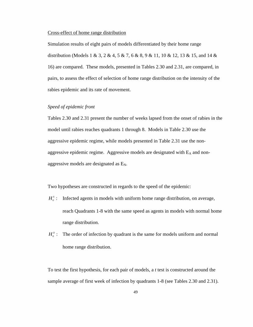
Cross-effect of home range distribution
Simulation results of eight pairs of models differentiated by their home range
distribution (Models 1 & 3, 2 & 4, 5 & 7, 6 & 8, 9 & 11, 10 & 12, 13 & 15, and 14 &
16) are compared. These models, presented in Tables 2.30 and 2.31, are compared, in
pairs, to assess the effect of selection of home range distribution on the intensity of the
rabies epidemic and its rate of movement.
Speed of epidemic front
Tables 2.30 and 2.31 present the number of weeks lapsed from the onset of rabies in the
model until rabies reaches quadrants 1 through 8. Models in Table 2.30 use the
aggressive epidemic regime, while models presented in Table 2.31 use the non-
aggressive epidemic regime. Aggressive models are designated with EA and non-
aggressive models are designated as EN.
Two hypotheses are constructed in regards to the speed of the epidemic:
:0SH Infected agents in models with uniform home range distribution, on average,
reach Quadrants 1-8 with the same speed as agents in models with normal home
range distribution.
:0OH The order of infection by quadrant is the same for models uniform and normal
home range distribution.
To test the first hypothesis, for each pair of models, a t test is constructed around the
sample average of first week of infection by quadrants 1-8 (see Tables 2.30 and 2.31).
49
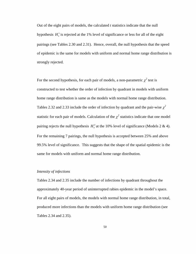
Out of the eight pairs of models, the calculated t statistics indicate that the null
hypothesis is rejected at the 1% level of significance or less for all of the eight
pairings (see Tables 2.30 and 2.31). Hence, overall, the null hypothesis that the speed
of epidemic is the same for models with uniform and normal home range distribution is
strongly rejected.
SH 0
50
.
For the second hypothesis, for each pair of models, a non-parametric χ2 test is
constructed to test whether the order of infection by quadrant in models with uniform
home range distribution is same as the models with normal home range distribution.
Tables 2.32 and 2.33 include the order of infection by quadrant and the pair-wise χ2
statistic for each pair of models. Calculation of the χ2 statistics indicate that one model
pairing rejects the null hypothesis O0 at the 10% level of significance (Models 2 & 4)
For the remaining 7 pairings, the null hypothesis is accepted between 25% and above
99.5% level of significance. This suggests that the shape of the spatial epidemic is the
same for models with uniform and normal home range distribution.
H
Intensity of infections
Tables 2.34 and 2.35 include the number of infections by quadrant throughout the
approximately 40-year period of uninterrupted rabies epidemic in the model’s space.
For all eight pairs of models, the models with normal home range distribution, in total,
produced more infections than the models with uniform home range distribution (see
Tables 2.34 and 2.35).
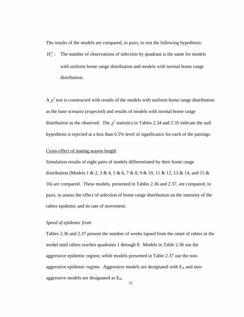
The results of the models are compared, in pairs, to test the following hypothesis:
:0OH The number of observations of infection by quadrant is the same for models
with uniform home range distribution and models with normal home range
distribution.
A χ2 test is constructed with results of the models with uniform home range distribution
as the base scenario (expected) and results of models with normal home range
distribution as the observed. The χ2 statistics in Tables 2.34 and 2.35 indicate the null
hypothesis is rejected at a less than 0.5% level of significance for each of the pairings.
Cross-effect of mating season length Simulation results of eight pairs of models differentiated by their home range
distribution (Models 1 & 2, 3 & 4, 5 & 6, 7 & 8, 9 & 10, 11 & 12, 13 & 14, and 15 &
16) are compared. These models, presented in Tables 2.36 and 2.37, are compared, in
pairs, to assess the effect of selection of home range distribution on the intensity of the
rabies epidemic and its rate of movement.
Speed of epidemic front
51
Tables 2.36 and 2.37 present the number of weeks lapsed from the onset of rabies in the
model until rabies reaches quadrants 1 through 8. Models in Table 2.36 use the
aggressive epidemic regime, while models presented in Table 2.37 use the non-
aggressive epidemic regime. Aggressive models are designated with EA and non-
aggressive models are designated as EN.
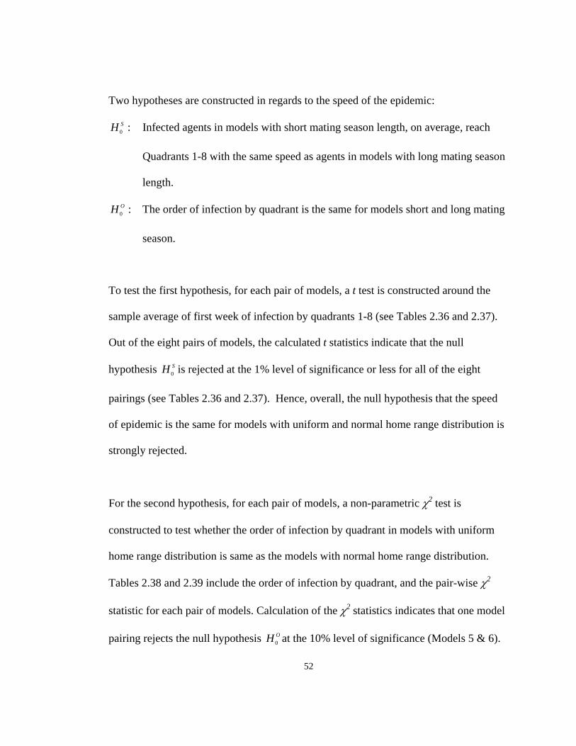
Two hypotheses are constructed in regards to the speed of the epidemic:
:0SH Infected agents in models with short mating season length, on average, reach
Quadrants 1-8 with the same speed as agents in models with long mating season
length.
:0OH The order of infection by quadrant is the same for models short and long mating
season.
52
t
To test the first hypothesis, for each pair of models, a t test is constructed around the
sample average of first week of infection by quadrants 1-8 (see Tables 2.36 and 2.37).
Out of the eight pairs of models, the calculated t statistics indicate that the null
hypothesis S is rejected at the 1% level of significance or less for all of the eigh
pairings (see Tables 2.36 and 2.37). Hence, overall, the null hypothesis that the speed
of epidemic is the same for models with uniform and normal home range distribution is
strongly rejected.
H 0
For the second hypothesis, for each pair of models, a non-parametric χ2 test is
constructed to test whether the order of infection by quadrant in models with uniform
home range distribution is same as the models with normal home range distribution.
Tables 2.38 and 2.39 include the order of infection by quadrant, and the pair-wise χ2
statistic for each pair of models. Calculation of the χ2 statistics indicates that one model
pairing rejects the null hypothesis at the 10% level of significance (Models 5 & 6). OH0
For the remaining 7 pairings, the null hypothesis is accepted between 50% and above
95% level of significance. This suggests that the shape of the spatial epidemic is the
same for models with uniform and normal home range distribution.
Intensity of infections
Tables 2.40 and 2.41 include the number of infections by quadrant throughout the
approximately 40-year period of uninterrupted rabies epidemic in the model’s space.
For all eight pairs of models, the models with normal home range distribution, in total,
produced more infections than the models with uniform home range distribution (see
Tables 2.40 and 2.41).
The results of the models are compared, in pairs, to test the following hypothesis:
:0OH The number of observations of infection by quadrant is the same for models
with short (13 weeks) and long (21 weeks) mating seasons.
A χ2 test is constructed with results of the models with uniform home range distribution
as the base scenario (expected) and results of models with normal home range
distribution as the observed. The χ2 statistics in Tables 2.40 and 2.41 indicate the null
hypothesis is rejected at a less than 0.5% level of significance for each of the pairings.
53
54
DISCUSSION
In this paper, I set out to develop a synthetic spatial environment and agents that mimic
the major characteristics of raccoons and their relation to their natural habitat. Certain
variables are altered to form different models to check the sensitivity of model results to
the variables used as well as finding the best model that fit raccoon ecology. The pre-
epidemic results indicate that while the order of population densities match the order of
density estimates found in raccoon ecology literature, their magnitude does not (see
Tables 2.1 and 2.3). Three explanations can be made regarding this difference:
1) The hypothetical environment does not represent reality well; hence, one can test a
geo-referenced environment to see if the difference in the magnitude of population
densities between simulation results and raccoon biology literature differ than those
found in the present model,
2) The description of the environment may be too simplistic. Inclusion of other
important variables such as roads that serve as paths of movement for raccoons may
lead to different results,
3) Parameterization of characteristics and behavior of raccoons may need to be
calibrated with the help of qualified raccoon biologists.
The pre-epidemic results also indicate that total population densities by land use
category is sensitive to choice of nutrient grow back algorithm (27% increase with
Urban grow back), home range distribution (13% increase with normal distribution),
and length of mating season (11% increase with the longer mating season). This
increase in total population densities eventually leads to higher incidences of raccoon
55
rabies once rabies is introduced to the model that may ultimately lead to higher
economic cost.
For the post-epidemic results, four variables (epidemic regime, nutrient grow back,
home range distribution, and length of mating season) are tested in regards to the rate of
movement and the shape of the epidemic front, and the intensity of epidemic in terms of
number of infections. Table 2.42 summarizes the effect of changes in variables on the
simulation results.
Changing the epidemic regime from an aggressive to a non-aggressive epidemic regime
(92% overall increase) had the most significant on the rate of movement of epidemic
front (Table 2.42). In the aggressive models, the initial rapid movement of the disease
serves as a culling instrument and consequently creates a barrier in form of low
population density. This result is in agreement with literature on disease movement in
that carrying capacity of susceptible population is the major factor in propagation of a
disease. Overall, the rate of movement decreases when the nutrient grow back
algorithm is changed from “Simple” to “Urban.” This phenomenon is due to the
clustering of raccoon agents in the Urban models. The agents become concentrated in
the urban spatial units where nutrients are abundant and grow back to capacity each
period after their nutrient is depleted. In contrast, in the Simple nutrient grow back
models, agents are spread out and serve as conduits for spread of disease. Changing the
variable from uniform to normal home range distribution, and from short to long mating
season length did not have significant effect on the rate of disease movement. Overall,
56
the order of first infection observed by quadrant (shape of the epidemic front) was not
affected by any variable changes. Hence, one can argue that the choice of environment
variables used in these models in conjunction with the agent variables is robust when it
comes to the shape of epidemic front. Overall, the intensity of disease epidemic in
terms of new infections increased as the model variables were changed from aggressive
to non-aggressive (32%), from Simple to Urban nutrient grow back algorithm (77%),
from uniform to normal home range distribution (19%) and from short to long mating
season length (23%). For home range distribution and mating season length, the
majority of increase in the intensity of infections can be explained by the effect the
change in these variables have on the increase of agent population in the pre-epidemic
period (see Table 2.42). The most significant increase in intensity of infection was due
to changing the nutrient grow back algorithm from Simple to Urban. Although this
change in variable resulted in a slower movement front of the epidemic, it resulted in
more new infections. As explained above, the clustering of agents to the more preferred
urban spatial units provided less opportunity for the disease to move, but at the same
time provided a cluster of susceptible agents for the infective agents. Hence, the disease
lingered in the spatial units for a longer period in the urban areas and increased the
likelihood of infection in these agent-concentrated areas.
Due to the time constraint, only one run of each model was simulated; hence, it should
be noted that these results should be considered with caution. It is advised that multiple
runs of each model be simulated and a confidence interval be constructed around the
results.
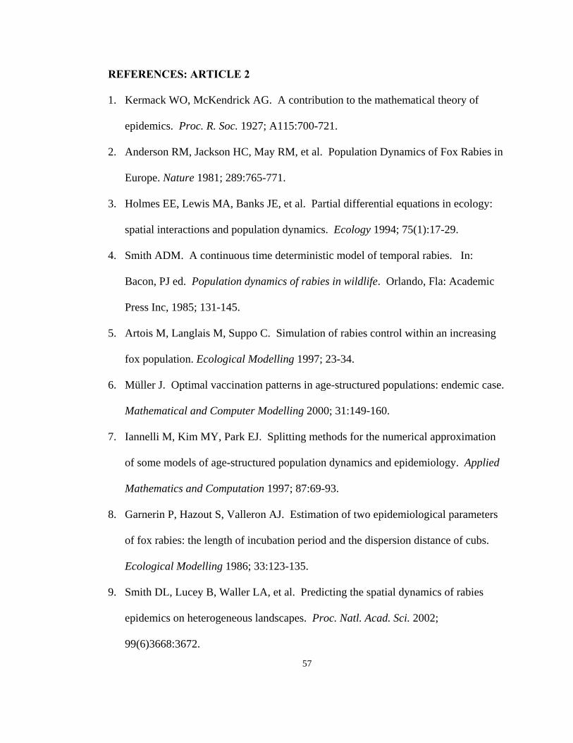
57
REFERENCES: ARTICLE 2
1. Kermack WO, McKendrick AG. A contribution to the mathematical theory of
epidemics. Proc. R. Soc. 1927; A115:700-721.
2. Anderson RM, Jackson HC, May RM, et al. Population Dynamics of Fox Rabies in
Europe. Nature 1981; 289:765-771.
3. Holmes EE, Lewis MA, Banks JE, et al. Partial differential equations in ecology:
spatial interactions and population dynamics. Ecology 1994; 75(1):17-29.
4. Smith ADM. A continuous time deterministic model of temporal rabies. In:
Bacon, PJ ed. Population dynamics of rabies in wildlife. Orlando, Fla: Academic
Press Inc, 1985; 131-145.
5. Artois M, Langlais M, Suppo C. Simulation of rabies control within an increasing
fox population. Ecological Modelling 1997; 23-34.
6. Müller J. Optimal vaccination patterns in age-structured populations: endemic case.
Mathematical and Computer Modelling 2000; 31:149-160.
7. Iannelli M, Kim MY, Park EJ. Splitting methods for the numerical approximation
of some models of age-structured population dynamics and epidemiology. Applied
Mathematics and Computation 1997; 87:69-93.
8. Garnerin P, Hazout S, Valleron AJ. Estimation of two epidemiological parameters
of fox rabies: the length of incubation period and the dispersion distance of cubs.
Ecological Modelling 1986; 33:123-135.
9. Smith DL, Lucey B, Waller LA, et al. Predicting the spatial dynamics of rabies
epidemics on heterogeneous landscapes. Proc. Natl. Acad. Sci. 2002;
99(6)3668:3672.
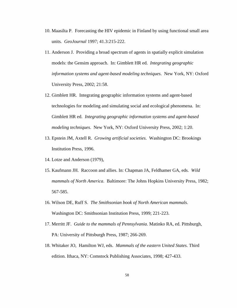
58
10. Maasilta P. Forecasting the HIV epidemic in Finland by using functional small area
units. GeoJournal 1997; 41.3:215-222.
11. Anderson J. Providing a broad spectrum of agents in spatially explicit simulation
models: the Gensim approach. In: Gimblett HR ed. Integrating geographic
information systems and agent-based modeling techniques. New York, NY: Oxford
University Press, 2002; 21:58.
12. Gimblett HR. Integrating geographic information systems and agent-based
technologies for modeling and simulating social and ecological phenomena. In:
Gimblett HR ed. Integrating geographic information systems and agent-based
modeling techniques. New York, NY: Oxford University Press, 2002; 1:20.
13. Epstein JM, Axtell R. Growing artificial societies. Washington DC: Brookings
Institution Press, 1996.
14. Lotze and Anderson (1979),
15. Kaufmann JH. Raccoon and allies. In: Chapman JA, Feldhamer GA, eds. Wild
mammals of North America. Baltimore: The Johns Hopkins University Press, 1982;
567-585.
16. Wilson DE, Ruff S. The Smithsonian book of North American mammals.
Washington DC: Smithsonian Institution Press, 1999; 221-223.
17. Merritt JF. Guide to the mammals of Pennsylvania. Matinko RA, ed. Pittsburgh,
PA: University of Pittsburgh Press, 1987; 266-269.
18. Whitaker JO, Hamilton WJ, eds. Mammals of the eastern United States. Third
edition. Ithaca, NY: Comstock Publishing Associates, 1998; 427-433.
59
19. Stuewer FE. Raccoons: their habits and management in Michigan. Ecological
Monographs, 13(2):205-256.
20. Sanderson GC, Nalbandov AV. The reproductive cycle of the raccoon in Illinois.
Illinois Natural History Survey Bulletin 1973. 31(2):29-84.
21. Nowak RM. Walker’s mammals of the world. Fifth Ed, Vol. II.. The Johns
Hopkins University Press, 1991; 1100-1101.
22. Winkler WG, Jenkins SR. Raccoon rabies. In: Baer GM, ed. The natural history of
rabies. 2nd ed. Boca Raton, Fla.: CRC Press Inc, 1991; 1991:325-340.
23. Uhaa IJ, Dato VM, Sorhage FE, et al. Benefits and costs of using an orally
absorbed vaccine to control rabies in raccoons. JAVMA, 201(12):1873-1882, 1992.
24. Noah DL, Smith MG, Gotthardt JC, et al. Mass human exposure to rabies in New
Hampshire: exposures, treatment, and cost.
25. Kreindel SM, McGuill M, Meltzer M, et al. The cost of rabies postexposure
prophylaxis: one state’s experience. Public Health Reports, 113:247-251, 1998.
26. Nelson RS, Cooper GH, Cartter ML, et al. Rabies postexposure prophylaxis –
Connecticut, 1990-1994. MMWR, 45(11):232-234, 1996.
27. Wyatt JD, Barker WH, Bennett NM, et al. Human rabies postexposure prophylaxis
during a raccoon rabies epizootic in New York, 1993 and 1994. Emerging
Infectious Diseases 1999, 5(3):415-423.
28. Kemere P, Liddel MK, Evangelou P, et al. Economic analysis of a large scale oral
vaccination program to control raccoon rabies. Unpublished Report, 1999.
Population density by land
Resolution
Nutrient Capacity
Nutrient Grow Back
Morbidity
Movement, Migration use
Reproduction
Environment Agent
Figure 2.1—Factors relating to the raccoon population density
0
0.1
0.2
0.3
0.4
0.5
0.6
Age (years)
Prob
abili
ty
probability 0.05 0.55 0.15 0.1 0.025 0.02 0.01 0.009 0.008 0.007 0.006 0.005 0.003 0.002 0.001
0 1 2 3 5 6 7 8 9 10 11 12 14 15 16
Figure 2.2—Probability distribution of age in wild raccoon population
60
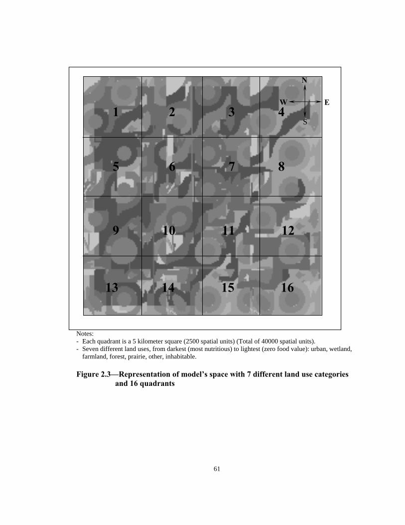
Notes:
1 2 3 4
5 6 7 8
9 10 11 12
13 14 15 16
N
W
S
E
- Each quadrant is a 5 kilometer square (2500 spatial units) (Total of 40000 spatial units). - Seven different land uses, from darkest (most nutritious) to lightest (zero food value): urban, wetland,
farmland, forest, prairie, other, inhabitable. Figure 2.3—Representation of model’s space with 7 different land use categories
and 16 quadrants
61

1.5 km
7 6 5 4 3 2 1 7 6 5 4 3 2 1 • 1 2 3 4 5 6 7 1.5 km 1 2 3 4 5 6 7
Figure 2.4—Home range potential of a raccoon agent with home range of 7 units (2.25 km2) in a 100 m2 cell lattice
62

0
0.2
0.4
0.6
0.8
1
1.2
0.09 0.25 0.49 0.81 1.21 1.69 2.25 2.89 3.61 4.41 5.29 6.25 7.29 8.41
Ho m e r an g e (k m 2)
Prob
abili
ty
c df N(7.5, 2) c df U(1, 14)
Notes: - cdf := cumulative distribution function - N(7.5, 2) := normal distribution with mean of 0.75 km and standard deviation of 0.2 km - U(1, 14) := uniform distribution with minimum of 0.1 km and maximum of 1.4 km Figure 2.5—Two possible home range distributions for the raccoon agents
63
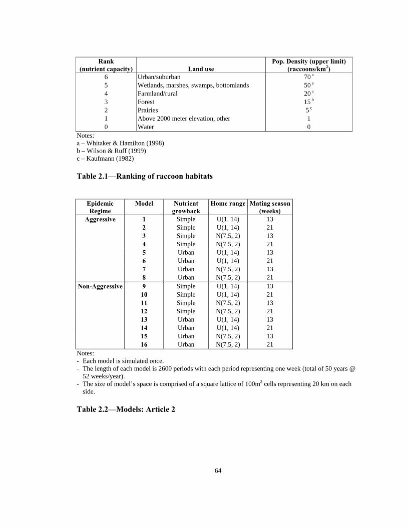
64
Rank
(nutrient capacity)
Land use Pop. Density (upper limit)
(raccoons/km2) 6 Urban/suburban 70 a
5 Wetlands, marshes, swamps, bottomlands 50 a
4 Farmland/rural 20 a
3 Forest 15 b
2 Prairies 5 c
1 Above 2000 meter elevation, other 1 0 Water 0
Notes: a – Whitaker & Hamilton (1998) b – Wilson & Ruff (1999) c – Kaufmann (1982) Table 2.1—Ranking of raccoon habitats
Epidemic Regime
Model Nutrient growback
Home range Mating season (weeks)
Aggressive 1 Simple U(1, 14) 13 2 Simple U(1, 14) 21 3 Simple N(7.5, 2) 13 4 Simple N(7.5, 2) 21 5 Urban U(1, 14) 13 6 Urban U(1, 14) 21 7 Urban N(7.5, 2) 13 8 Urban N(7.5, 2) 21
Non-Aggressive 9 Simple U(1, 14) 13 10 Simple U(1, 14) 21 11 Simple N(7.5, 2) 13 12 Simple N(7.5, 2) 21 13 Urban U(1, 14) 13 14 Urban U(1, 14) 21 15 Urban N(7.5, 2) 13 16 Urban N(7.5, 2) 21
Notes: - Each model is simulated once. - The length of each model is 2600 periods with each period representing one week (total of 50 years @
52 weeks/year). - The size of model’s space is comprised of a square lattice of 100m2 cells representing 20 km on each
side. Table 2.2—Models: Article 2
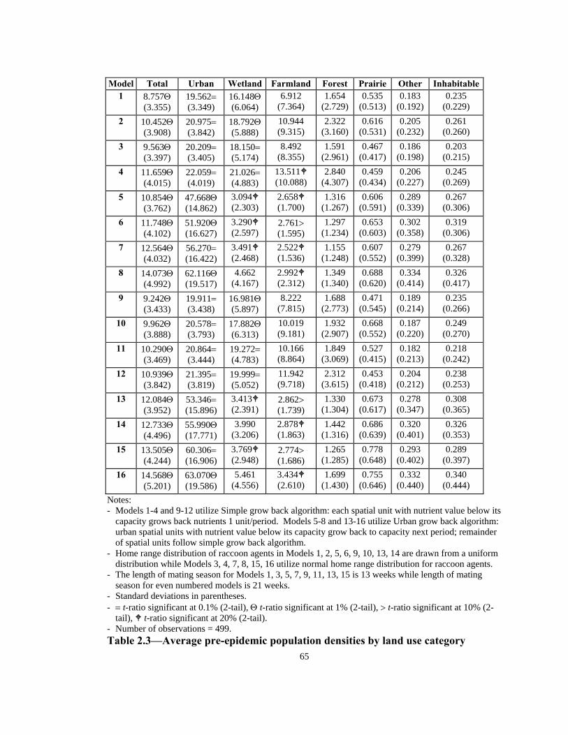
65
Model Total Urban Wetland Farmland Forest Prairie Other Inhabitable
1 8.757Θ (3.355)
19.562= (3.349)
16.148Θ (6.064)
6.912 (7.364)
1.654 (2.729)
0.535 (0.513)
0.183 (0.192)
0.235 (0.229)
2 10.452Θ (3.908)
20.975= (3.842)
18.792Θ (5.888)
10.944 (9.315)
2.322 (3.160)
0.616 (0.531)
0.205 (0.232)
0.261 (0.260)
3 9.563Θ (3.397)
20.209= (3.405)
18.150= (5.174)
8.492 (8.355)
1.591 (2.961)
0.467 (0.417)
0.186 (0.198)
0.203 (0.215)
4 11.659Θ (4.015)
22.059= (4.019)
21.026= (4.883)
13.511 (10.088)
2.840 (4.307)
0.459 (0.434)
0.206 (0.227)
0.245 (0.269)
5 10.854Θ (3.762)
47.668Θ (14.862)
3.094 (2.303)
2.658 (1.700)
1.316 (1.267)
0.606 (0.591)
0.289 (0.339)
0.267 (0.306)
6 11.748Θ (4.102)
51.920Θ (16.627)
3.290 (2.597)
2.761> (1.595)
1.297 (1.234)
0.653 (0.603)
0.302 (0.358)
0.319 (0.306)
7 12.564Θ (4.032)
56.270= (16.422)
3.491 (2.468)
2.522 (1.536)
1.155 (1.248)
0.607 (0.552)
0.279 (0.399)
0.267 (0.328)
8 14.073Θ (4.992)
62.116Θ (19.517)
4.662 (4.167)
2.992 (2.312)
1.349 (1.340)
0.688 (0.620)
0.334 (0.414)
0.326 (0.417)
9 9.242Θ (3.433)
19.911= (3.438)
16.981Θ (5.897)
8.222 (7.815)
1.688 (2.773)
0.471 (0.545)
0.189 (0.214)
0.235 (0.266)
10 9.962Θ (3.888)
20.578= (3.793)
17.882Θ (6.313)
10.019 (9.181)
1.932 (2.907)
0.668 (0.552)
0.187 (0.220)
0.249 (0.270)
11 10.290Θ (3.469)
20.864= (3.444)
19.272= (4.783)
10.166 (8.864)
1.849 (3.069)
0.527 (0.415)
0.182 (0.213)
0.218 (0.242)
12 10.939Θ (3.842)
21.395= (3.819)
19.999= (5.052)
11.942 (9.718)
2.312 (3.615)
0.453 (0.418)
0.204 (0.212)
0.238 (0.253)
13 12.084Θ (3.952)
53.346= (15.896)
3.413 (2.391)
2.862> (1.739)
1.330 (1.304)
0.673 (0.617)
0.278 (0.347)
0.308 (0.365)
14 12.733Θ (4.496)
55.990Θ (17.771)
3.990 (3.206)
2.878 (1.863)
1.442 (1.316)
0.686 (0.639)
0.320 (0.401)
0.326 (0.353)
15 13.505Θ (4.244)
60.306= (16.906)
3.769 (2.948)
2.774> (1.686)
1.265 (1.285)
0.778 (0.648)
0.293 (0.402)
0.289 (0.397)
16 14.568Θ (5.201)
63.070Θ (19.586)
5.461 (4.556)
3.434 (2.610)
1.699 (1.430)
0.755 (0.646)
0.332 (0.440)
0.340 (0.444)
Notes: - Models 1-4 and 9-12 utilize Simple grow back algorithm: each spatial unit with nutrient value below its
capacity grows back nutrients 1 unit/period. Models 5-8 and 13-16 utilize Urban grow back algorithm: urban spatial units with nutrient value below its capacity grow back to capacity next period; remainder of spatial units follow simple grow back algorithm.
- Home range distribution of raccoon agents in Models 1, 2, 5, 6, 9, 10, 13, 14 are drawn from a uniform distribution while Models 3, 4, 7, 8, 15, 16 utilize normal home range distribution for raccoon agents.
- The length of mating season for Models 1, 3, 5, 7, 9, 11, 13, 15 is 13 weeks while length of mating season for even numbered models is 21 weeks.
- Standard deviations in parentheses. - = t-ratio significant at 0.1% (2-tail), Θ t-ratio significant at 1% (2-tail), > t-ratio significant at 10% (2-
tail), t-ratio significant at 20% (2-tail). - Number of observations = 499. Table 2.3—Average pre-epidemic population densities by land use category
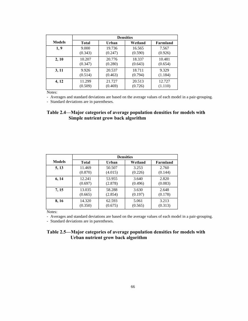
66
Densities
Models Total Urban Wetland Farmland 1, 9 9.000
(0.343) 19.736 (0.247)
16.565 (0.590)
7.567 (0.926)
2, 10 10.207 (0.347)
20.776 (0.280)
18.337 (0.643)
10.481 (0.654)
3, 11 9.926 (0.514)
20.537 (0.463)
18.711 (0.794)
9.329 (1.184)
4, 12 11.299 (0.509)
21.727 (0.469)
20.513 (0.726)
12.727 (1.110)
Notes: - Averages and standard deviations are based on the average values of each model in a pair-grouping. - Standard deviations are in parentheses. Table 2.4—Major categories of average population densities for models with
Simple nutrient grow back algorithm
Densities Models Total Urban Wetland Farmland
5, 13 11.469 (0.870)
50.507 (4.015)
3.253 (0.226)
2.760 (0.144)
6, 14 12.241 (0.697)
53.955 (2.878)
3.640 (0.496)
2.820 (0.083)
7, 15 13.035 (0.665)
58.288 (2.854)
3.630 (0.197)
2.648 (0.178)
8, 16 14.320 (0.350)
62.593 (0.675)
5.061 (0.565)
3.213 (0.313)
Notes: - Averages and standard deviations are based on the average values of each model in a pair-grouping. - Standard deviations are in parentheses. Table 2.5—Major categories of average population densities for models with
Urban nutrient grow back algorithm
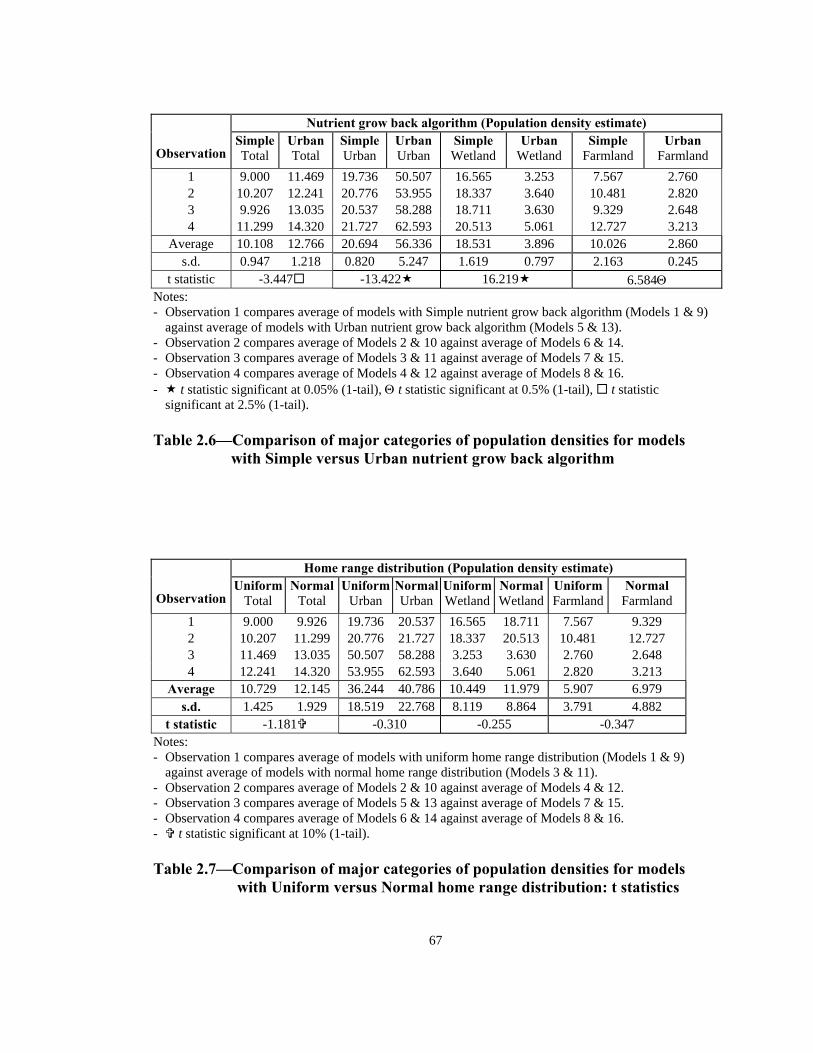
67
Nutrient grow back algorithm (Population density estimate)
Observation
Simple Total
Urban Total
SimpleUrban
Urban Urban
Simple Wetland
Urban Wetland
Simple Farmland
Urban Farmland
1 9.000 11.469 19.736 50.507 16.565 3.253 7.567 2.760 2 10.207 12.241 20.776 53.955 18.337 3.640 10.481 2.820 3 9.926 13.035 20.537 58.288 18.711 3.630 9.329 2.648 4 11.299 14.320 21.727 62.593 20.513 5.061 12.727 3.213
Average 10.108 12.766 20.694 56.336 18.531 3.896 10.026 2.860 s.d. 0.947 1.218 0.820 5.247 1.619 0.797 2.163 0.245
t statistic -3.447 -13.422 16.219 6.584Θ Notes: - Observation 1 compares average of models with Simple nutrient grow back algorithm (Models 1 & 9)
against average of models with Urban nutrient grow back algorithm (Models 5 & 13). - Observation 2 compares average of Models 2 & 10 against average of Models 6 & 14. - Observation 3 compares average of Models 3 & 11 against average of Models 7 & 15. - Observation 4 compares average of Models 4 & 12 against average of Models 8 & 16. - t statistic significant at 0.05% (1-tail), Θ t statistic significant at 0.5% (1-tail), t statistic
significant at 2.5% (1-tail). Table 2.6—Comparison of major categories of population densities for models
with Simple versus Urban nutrient grow back algorithm
Home range distribution (Population density estimate)
Observation Uniform
Total Normal
Total Uniform
Urban NormalUrban
UniformWetland
NormalWetland
Uniform Farmland
Normal Farmland
1 9.000 9.926 19.736 20.537 16.565 18.711 7.567 9.329 2 10.207 11.299 20.776 21.727 18.337 20.513 10.481 12.727 3 11.469 13.035 50.507 58.288 3.253 3.630 2.760 2.648 4 12.241 14.320 53.955 62.593 3.640 5.061 2.820 3.213
Average 10.729 12.145 36.244 40.786 10.449 11.979 5.907 6.979 s.d. 1.425 1.929 18.519 22.768 8.119 8.864 3.791 4.882
t statistic -1.181 -0.310 -0.255 -0.347 Notes: - Observation 1 compares average of models with uniform home range distribution (Models 1 & 9)
against average of models with normal home range distribution (Models 3 & 11). - Observation 2 compares average of Models 2 & 10 against average of Models 4 & 12. - Observation 3 compares average of Models 5 & 13 against average of Models 7 & 15. - Observation 4 compares average of Models 6 & 14 against average of Models 8 & 16. - t statistic significant at 10% (1-tail). Table 2.7—Comparison of major categories of population densities for models
with Uniform versus Normal home range distribution: t statistics

68
Models
1, 3 9, 11 2, 4 10, 12 5, 7 13, 15 6, 8 14, 16 Nutrient grow back algorithm →
Simple Simple Simple Simple Urban Urban Urban Urban
Mating season → 13 weeks 13 weeks 21 weeks 21 weeks 13 weeks 13 weeks 21 weeks 21 weeksLand use category Total -3.769 -4.793 -4.811 -3.994 -6.930 -5.475 -8.038 -5.961Urban -3.029 -4.374 -4.355 -3.388 -8.676 -6.700 -8.883 -5.980Wetland -5.611 -6.739 -6.523 -5.850 -2.628Θ -2.094> -6.243 -5.895Farmland -3.169 -3.675 -4.177 -3.214 1.325 0.808Φ -1.834 -3.870Notes: - Each pair of model includes one model with uniform home range distribution and another with normal
home range distribution. See Table 2.2 for key. - Z statistic significant at 0.1% (1-tail), Θ Z statistic significant at 0.5% (1-tail), > Z statistic
significant at 2.5% (1-tail), Z statistic significant at 5% (1-tail), Z statistic significant at 10% (1-tail), Φ Z statistic significant at 25% (1-tail).
Table 2.8—Comparison of major categories of population densities for pairs of
models with uniform versus normal home range distribution: Z statistics
Models 1, 3 9, 11 2, 4 10, 12 5, 7 13, 15 6, 8 14, 16
Nutrient grow back algorithm → Simple Simple Simple Simple Urban Urban Urban Urban
Home range → Uniform Uniform Normal Normal Uniform Uniform Normal Normal Land use category Total -7.350 -3.098 -8.901 -2.802Θ -3.589 -2.424 -5.251 -3.537Urban -6.193 -2.912Θ -7.842 -2.305> -4.259 -2.477 -5.119 -2.386Wetland -6.990 -2.329 -9.030 -2.335 -1.260Φ -3.224 -5.401 -6.964Farmland -7.584 -3.329 -8.560 -3.017Θ -0.985Φ -0.142 -3.777 -4.740Notes: - Each pair of model includes one model with a short mating season (13 weeks) and another with long
mating season (21 weeks). See Table 2.2 for key. - Z statistic significant at 0.1% (1-tail), Θ Z statistic significant at 0.5% (1-tail), Z statistic
significant at 1% (1-tail), > Z statistic significant at 2.5% (1-tail), Z statistic significant at 10% (1-tail), Φ Z statistic significant at 25% (1-tail).
Table 2.9—Comparison of major categories of population densities for pairs of
models with 13-week versus 21-week mating season: Z statistics

69
Model 1 Model 9
Densities average s.d. average s.d. Ζ
Accept null hypothesis, α = 0.01
Total 8.757 3.355 9.242 3.433 2.259 Yes Urban 19.562 3.349 19.911 3.438 -1.627 Yes Wetland 16.148 6.064 16.981 5.897 2.203 Yes Farmland 6.912 7.364 8.222 7.815 2.724 No Forest 1.654 2.729 1.688 2.773 0.192 Yes Prairie 0.535 0.513 0.471 0.545 -1.903 Yes Other 0.183 0.192 0.189 0.214 0.405 Yes Water 0.235 0.229 0.235 0.266 0.013 Yes Note: - Null hypothesis: sample means of models are not significantly different from each other. Table 2.10—Consistency of models with Simple nutrient grow back algorithm,
uniform home range distribution and 13-week mating season: Z statistics
Model 2 Model 10 Densities average s.d. average s.d.
Ζ
Accept null hypothesis, α = 0.01
Total 10.452 3.908 9.962 3.888 1.986 Yes Urban 20.975 3.842 20.578 3.793 1.639 Yes Wetland 18.792 5.888 17.882 6.313 2.355 No Farmland 10.944 9.315 10.019 9.181 1.580 Yes Forest 2.322 3.160 1.932 2.907 2.031 Yes Prairie 0.616 0.531 0.668 0.552 -1.518 Yes Other 0.205 0.232 0.187 0.220 1.211 Yes Water 0.261 0.260 0.249 0.270 0.734 Yes Note: - Null hypothesis: sample means of models are not significantly different from each other. Table 2.11—Consistency of models with Simple nutrient grow back algorithm,
uniform home range distribution and 21-week mating season: Z statistics
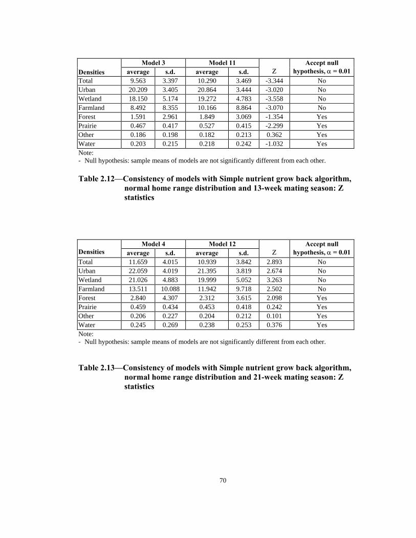
70
Model 3 Model 11
Densities average s.d. average s.d. Ζ
Accept null hypothesis, α = 0.01
Total 9.563 3.397 10.290 3.469 -3.344 No Urban 20.209 3.405 20.864 3.444 -3.020 No Wetland 18.150 5.174 19.272 4.783 -3.558 No Farmland 8.492 8.355 10.166 8.864 -3.070 No Forest 1.591 2.961 1.849 3.069 -1.354 Yes Prairie 0.467 0.417 0.527 0.415 -2.299 Yes Other 0.186 0.198 0.182 0.213 0.362 Yes Water 0.203 0.215 0.218 0.242 -1.032 Yes Note: - Null hypothesis: sample means of models are not significantly different from each other. Table 2.12—Consistency of models with Simple nutrient grow back algorithm,
normal home range distribution and 13-week mating season: Z statistics
Model 4 Model 12 Densities average s.d. average s.d.
Ζ
Accept null hypothesis, α = 0.01
Total 11.659 4.015 10.939 3.842 2.893 No Urban 22.059 4.019 21.395 3.819 2.674 No Wetland 21.026 4.883 19.999 5.052 3.263 No Farmland 13.511 10.088 11.942 9.718 2.502 No Forest 2.840 4.307 2.312 3.615 2.098 Yes Prairie 0.459 0.434 0.453 0.418 0.242 Yes Other 0.206 0.227 0.204 0.212 0.101 Yes Water 0.245 0.269 0.238 0.253 0.376 Yes Note: - Null hypothesis: sample means of models are not significantly different from each other. Table 2.13—Consistency of models with Simple nutrient grow back algorithm,
normal home range distribution and 21-week mating season: Z statistics
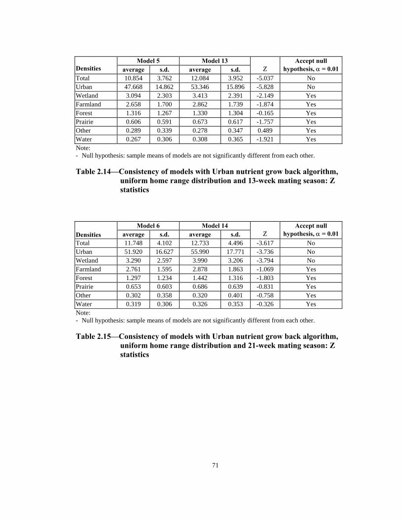
71
Model 5 Model 13
Densities average s.d. average s.d. Ζ
Accept null hypothesis, α = 0.01
Total 10.854 3.762 12.084 3.952 -5.037 No Urban 47.668 14.862 53.346 15.896 -5.828 No Wetland 3.094 2.303 3.413 2.391 -2.149 Yes Farmland 2.658 1.700 2.862 1.739 -1.874 Yes Forest 1.316 1.267 1.330 1.304 -0.165 Yes Prairie 0.606 0.591 0.673 0.617 -1.757 Yes Other 0.289 0.339 0.278 0.347 0.489 Yes Water 0.267 0.306 0.308 0.365 -1.921 Yes Note: - Null hypothesis: sample means of models are not significantly different from each other. Table 2.14—Consistency of models with Urban nutrient grow back algorithm,
uniform home range distribution and 13-week mating season: Z statistics
Model 6 Model 14 Densities average s.d. average s.d.
Ζ
Accept null hypothesis, α = 0.01
Total 11.748 4.102 12.733 4.496 -3.617 No Urban 51.920 16.627 55.990 17.771 -3.736 No Wetland 3.290 2.597 3.990 3.206 -3.794 No Farmland 2.761 1.595 2.878 1.863 -1.069 Yes Forest 1.297 1.234 1.442 1.316 -1.803 Yes Prairie 0.653 0.603 0.686 0.639 -0.831 Yes Other 0.302 0.358 0.320 0.401 -0.758 Yes Water 0.319 0.306 0.326 0.353 -0.326 Yes Note: - Null hypothesis: sample means of models are not significantly different from each other. Table 2.15—Consistency of models with Urban nutrient grow back algorithm,
uniform home range distribution and 21-week mating season: Z statistics
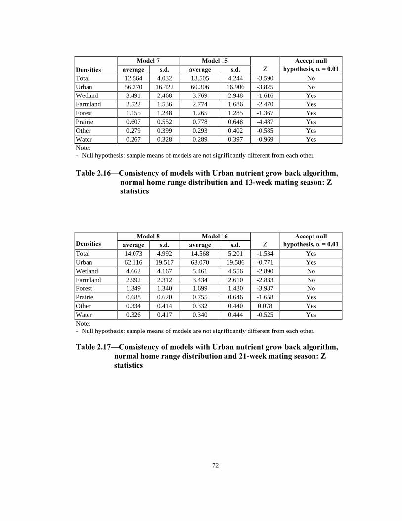
72
Model 7 Model 15
Densities average s.d. average s.d. Ζ
Accept null hypothesis, α = 0.01
Total 12.564 4.032 13.505 4.244 -3.590 No Urban 56.270 16.422 60.306 16.906 -3.825 No Wetland 3.491 2.468 3.769 2.948 -1.616 Yes Farmland 2.522 1.536 2.774 1.686 -2.470 Yes Forest 1.155 1.248 1.265 1.285 -1.367 Yes Prairie 0.607 0.552 0.778 0.648 -4.487 Yes Other 0.279 0.399 0.293 0.402 -0.585 Yes Water 0.267 0.328 0.289 0.397 -0.969 Yes Note: - Null hypothesis: sample means of models are not significantly different from each other. Table 2.16—Consistency of models with Urban nutrient grow back algorithm,
normal home range distribution and 13-week mating season: Z statistics
Model 8 Model 16 Densities average s.d. average s.d.
Ζ
Accept null hypothesis, α = 0.01
Total 14.073 4.992 14.568 5.201 -1.534 Yes Urban 62.116 19.517 63.070 19.586 -0.771 Yes Wetland 4.662 4.167 5.461 4.556 -2.890 No Farmland 2.992 2.312 3.434 2.610 -2.833 No Forest 1.349 1.340 1.699 1.430 -3.987 No Prairie 0.688 0.620 0.755 0.646 -1.658 Yes Other 0.334 0.414 0.332 0.440 0.078 Yes Water 0.326 0.417 0.340 0.444 -0.525 Yes Note: - Null hypothesis: sample means of models are not significantly different from each other. Table 2.17—Consistency of models with Urban nutrient grow back algorithm,
normal home range distribution and 21-week mating season: Z statistics

Models
1 9 2 10 3 11 4 12 Nutrient grow back algorithm → Simple Simple Simple Simple Simple Simple Simple Simple
Epidemic regime → EA EN EA EN EA EN EA ENQuadrant
1 55 79 67 60 82 97 52 127 2 42 81 63 49 68 111 53 123 3 42 105 64 63 56 112 56 135 4 50 155 89 80 44 190 85 147 5 44 57 47 34 32 78 38 69 6 30 79 45 33 36 71 39 65 7 28 93 46 44 30 77 37 86 8 40 108 58 70 38 111 35 113
average 41.375 94.625 59.875 54.125 48.250 105.875 49.375 108.125s.d. 9.086 29.335 14.682 16.966 18.745 37.934 16.604 30.972
t -4.904 0.725 -3.852 -4.729 Rejection level of SH 0 0.1% 25% 0.5% 0.5%
Note: - Null hypothesis: infected agents in non-aggressive models, on average, reach quadrants 1-8 with the
same speed as those agents in the aggressive models. - Note: Each group of models contains two independent samples. - 7 degrees of freedom rejection level.
Table 2.18— Number of weeks lapsed after onset of rabies until its appearance by
quadrant (1 through 8) in models with Simple nutrient grow back algorithm: aggressive vs. non-aggressive epidemic regimes
73

Models
5 13 6 14 7 15 8 16 Nutrient grow back algorithm → Urban Urban Urban Urban Urban Urban Urban Urban
Epidemic regime → EA EN EA EN EA EN EA ENQuadrant
1 63 191 88 89 66 146 60 97 2 59 188 85 90 74 154 53 92 3 57 203 93 108 85 158 58 92 4 56 198 93 135 82 170 70 99 5 43 93 58 58 48 104 47 62 6 39 139 57 61 51 104 46 61 7 35 167 64 103 56 122 52 68 8 44 196 58 121 59 154 59 89
average 49.500 171.875 74.500 95.625 65.125 139.000 55.625 82.500 s.d. 10.447 38.144 16.639 26.971 14.004 25.523 7.836 16.027
t -8.752 -1.885 -7.177 -4.261 Rejection level of SH 0 0.1% 10% 0.1% 0.5%
N te: - Null hypothesis: infected agents in non-aggressive models, on average, reach quadrants 1-8 with the
o
same speed as those agents in the aggressive models. wo independent samples. - Note: Each group of models contains t
7 degrees of freedom rejection level. - Table 2.19— Number of weeks lapsed after onset of rabies until its appearance by
quadrant (1 through 8) in models with Urban nutrient grow back algorithm: aggressive vs. non-aggressive epidemic regimes
74
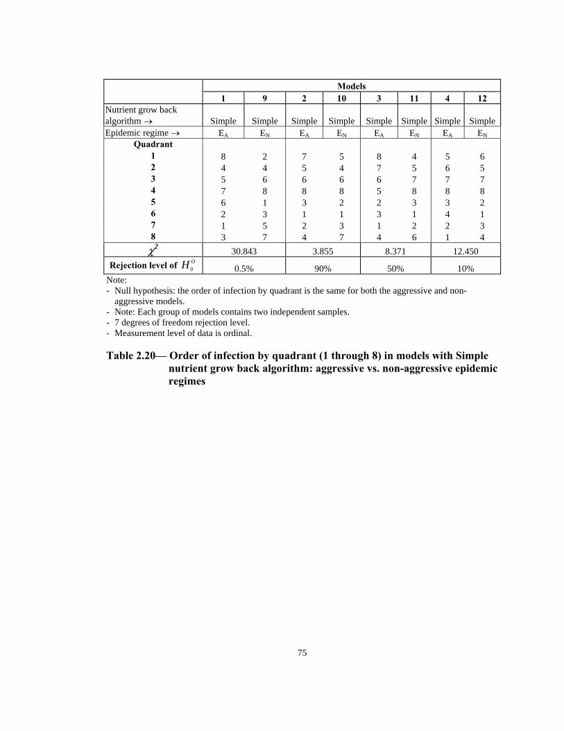
Models
1 9 2 10 3 11 4 12 Nutrient grow back algorithm → Simple Simple Simple Simple Simple Simple Simple Simple Epidemic regime → EA EN EA EN EA EN EA EN
Quadrant 1 8 2 7 5 8 4 5 6 2 4 4 5 4 7 5 6 5 3 5 6 6 6 6 7 7 7 4 7 8 8 8 5 8 8 8 5 6 1 3 2 2 3 3 2 6 2 3 1 1 3 1 4 1 7 1 5 2 3 1 2 2 3 8 3 7 4 7 4 6 1 4 χ2 30.843 3.855 8.371 12.450
Rejection level of OH 0 0.5% 90% 50% 10% Note: - Null hypothesis: the order of infection by quadrant is the same for both the aggressive and non-
aggressive models. - Note: Each group of models contains two independent samples. - 7 degrees of freedom rejection level. - Measurement level of data is ordinal.
Table 2.20— Order of infection by quadrant (1 through 8) in models with Simple
nutrient grow back algorithm: aggressive vs. non-aggressive epidemic regimes
75

Models
5 13 6 14 7 15 8 16 Nutrient grow back algorithm → Urban Urban Urban Urban Urban Urban Urban Urban
Epidemic regime → EA EN EA EN EA EN EA ENQuadrant
1 8 5 6 3 5 4 7 7 2 7 4 5 4 6 5 4 5 3 6 8 7 6 8 7 5 6 4 5 7 8 8 7 8 8 8 5 3 1 2 1 1 1 2 2 6 2 2 1 2 2 2 1 1 7 1 3 4 5 3 3 3 3 8 4 6 3 7 4 6 6 4 χ2 10.211 8.926 1.635 1.117
Rejection level of OH 0 25% 50% 99% 99.5% N te: - Null hypothesis: the order of infection by quadrant is the same for both the aggressive and non-
o
aggressive models. wo independent samples. - Note: Each group of models contains t
- 7 degrees of freedom rejection level. - Measurement level of data is ordinal.
Table 2.21—Order of infection by quadrant (1 through 8) in models with Urban
nutrient grow back algorithm: aggressive vs. non- aggressive epidemic regimes
76

Models
1 9 2 10 3 11 4 12 Nutrient grow back algorithm → Simple Simple Simple Simple Simple Simple Simple Simple
Epidemic regime → EA EN EA EN EA EN EA ENQuadrant
1 849 724 878 1104 1025 2447 1144 1151 2 395 312 749 740 368 1033 608 549 3 687 232 1239 1349 816 497 956 368 4 245 53 114 328 434 59 10 7 5 1319 1508 1604 2114 1863 3104 2196 2596 6 1133 1679 2440 2185 1598 2622 1558 2182 7 618 1083 1065 2340 987 1817 1389 1986 8 68 89 146 196 202 147 227 133
Totals 5,314 8,235 7,293 8,088 9,777 12,424 12,598 15,270 χ2 1134.22 2202.10 5818.99 986.62
Rejection level of OH 0 <0.5% <0.5% <0.5% <0.5% Note: - Null hypothesis: the number of infection by quadrant is the same for both the aggressive and non-
aggressive models. - Note: Each group of models contains two independent samples. - Critical value for the non-parametric chi-square test is 24.32 for α = 0.001 (d.f. = 7). Table 2.22—Number of infections by quadrant in models with Simple nutrient
grow back algorithm: aggressive versus non-aggressive epidemic regimes
77
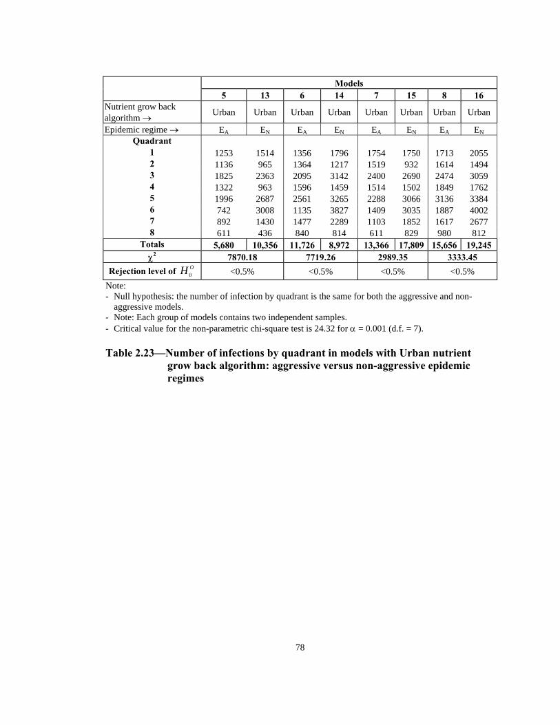
Models
5 13 6 14 7 15 8 16 Nutrient grow back algorithm → Urban Urban Urban Urban Urban Urban Urban Urban
Epidemic regime → EA EN EA EN EA EN EA ENQuadrant
1 1253 1514 1356 1796 1754 1750 1713 2055 2 1136 965 1364 1217 1519 932 1614 1494 3 1825 2363 2095 3142 2400 2690 2474 3059 4 1322 963 1596 1459 1514 1502 1849 1762 5 1996 2687 2561 3265 2288 3066 3136 3384 6 742 3008 1135 3827 1409 3035 1887 4002 7 892 1430 1477 2289 1103 1852 1617 2677 8 611 436 840 814 611 829 980 812
Totals 5,680 10,356 11,726 8,972 13,366 17,809 15,656 19,245 χ2 7870.18 7719.26 2989.35 3333.45
Rejection level of OH 0 <0.5% <0.5% <0.5% <0.5% N te: - Null hypothesis: the number of infection by quadrant is the same for both the aggressive and non-
o
aggressive models. - Note: Each group of models contains two independent samples. Critical value for the non-parametric chi-square test is 24.32 for α = 0.001 (d.f. = 7). -
Table 2.23—Number of infections by quadrant in models with Urban nutrient
grow back algorithm: aggressive versus non-aggressive epidemic regimes
78
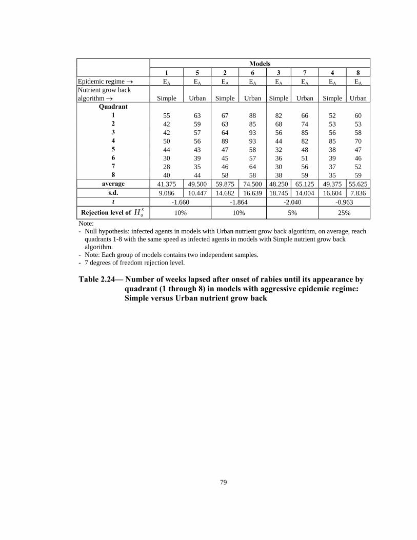
Models
1 5 2 6 3 7 4 8 Epidemic regime → EA EA EA EA EA EA EA EA
Nutrient grow back algorithm → Simple Urban Simple Urban Simple Urban Simple Urban
Quadrant 1 55 63 67 88 82 66 52 60 2 42 59 63 85 68 74 53 53 3 42 57 64 93 56 85 56 58 4 50 56 89 93 44 82 85 70 5 44 43 47 58 32 48 38 47 6 30 39 45 57 36 51 39 46 7 28 35 46 64 30 56 37 52 8 40 44 58 58 38 59 35 59
average 41.375 49.500 59.875 74.500 48.250 65.125 49.375 55.625s.d. 9.086 10.447 14.682 16.639 18.745 14.004 16.604 7.836
t -1.660 -1.864 -2.040 -0.963 Rejection level of SH 0 10% 10% 5% 25%
Note: - Null hypothesis: infected agents in models with Urban nutrient grow back algorithm, on average, reach
quadrants 1-8 with the same speed as infected agents in models with Simple nutrient grow back algorithm.
- Note: Each group of models contains two independent samples. - 7 degrees of freedom rejection level.
Table 2.24— Number of weeks lapsed after onset of rabies until its appearance by
quadrant (1 through 8) in models with aggressive epidemic regime: Simple versus Urban nutrient grow back
79

Models
9 13 10 14 11 15 12 16 Epidemic regime → EN EN EN EN EN EN EN EN
Nutrient grow back algorithm → Simple Urban Simple Urban Simple Urban Simple Urban
Quadrant 1 79 191 60 89 97 146 127 97 2 81 188 49 90 111 154 123 92 3 105 203 63 108 112 158 135 92 4 155 198 80 135 190 170 147 99 5 57 93 34 58 78 104 69 62 6 79 139 33 61 71 104 65 61 7 93 167 44 103 77 122 86 68 8 108 196 70 121 111 154 113 89
average 94.625 171.875 54.125 95.625 105.875 139.000 108.125 82.500s.d. 29.335 38.144 16.966 26.971 37.934 25.523 30.972 16.027T -4.541 -3.684 -2.049 2.078
Rejection level of SH 0 0.5% 0.5% 5% 5% N te: - Null hypothesis: infected agents in models with Urban nutrient grow back algorithm, on average, reach
quadrants 1-8 with the same speed as infected agents in models with Simple nutrient grow back
o
algorithm. wo independent samples. - Note: Each group of models contains t
- 7 de rees of freedom rejection level. g
Table 2.25— Number of weeks lapsed after onset of rabies until its appearance by quadrant (1 through 8) in models with non-aggressive epidemic
regime: Simple versus Urban nutrient grow back
80
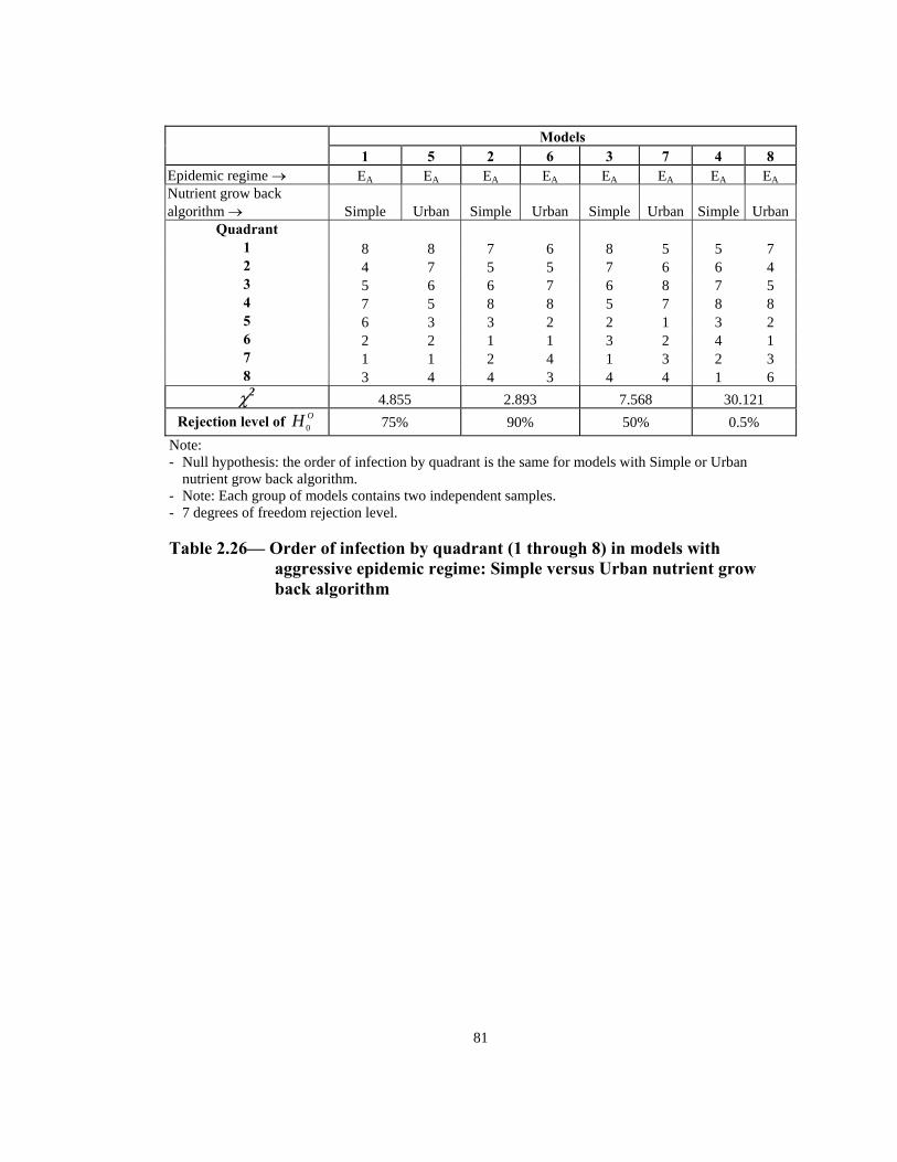
Models
1 5 2 6 3 7 4 8 Epidemic regime → EA EA EA EA EA EA EA EANutrient grow back algorithm → Simple Urban Simple Urban Simple Urban Simple Urban
Quadrant 1 8 8 7 6 8 5 5 7 2 4 7 5 5 7 6 6 4 3 5 6 6 7 6 8 7 5 4 7 5 8 8 5 7 8 8 5 6 3 3 2 2 1 3 2 6 2 2 1 1 3 2 4 1 7 1 1 2 4 1 3 2 3 8 3 4 4 3 4 4 1 6 χ2 4.855 2.893 7.568 30.121
Rejection level of OH0 75% 90% 50% 0.5% Note: - Null hypothesis: the order of infection by quadrant is the same for models with Simple or Urban
nutrient grow back algorithm. - Note: Each group of models contains two independent samples. - 7 degrees of freedom rejection level.
Table 2.26— Order of infection by quadrant (1 through 8) in models with
aggressive epidemic regime: Simple versus Urban nutrient grow back algorithm
81

Models
9 13 10 14 11 15 12 16 Epidemic regime → EN EN EN EN EN EN EN ENNutrient grow back algorithm → Simple Urban Simple Urban Simple Urban Simple Urban
Quadrant 1 2 5 5 3 4 4 6 7 2 4 4 4 4 5 5 5 5 3 6 8 6 6 7 7 7 6 4 8 7 8 8 8 8 8 8 5 1 1 2 1 3 1 2 2 6 3 2 1 2 1 2 1 1 7 5 3 3 5 2 3 3 3 8 7 6 7 7 6 6 4 4 χ2 6.568 3.633 2.833 0.310
Rejection level of OH0 50% 90% 90% 99.5% N te: - Null hypothesis: the order of infection by quadrant is the same for models with Simple or Urban
o
nutrient grow back algorithm. wo independent samples. - Note: Each group of models contains t
7 degrees of freedom rejection level. - Table 2.27— Order of infection by quadrant (1 through 8) in models with non-
aggressive epidemic regime: Simple versus Urban nutrient grow back algorithm
82
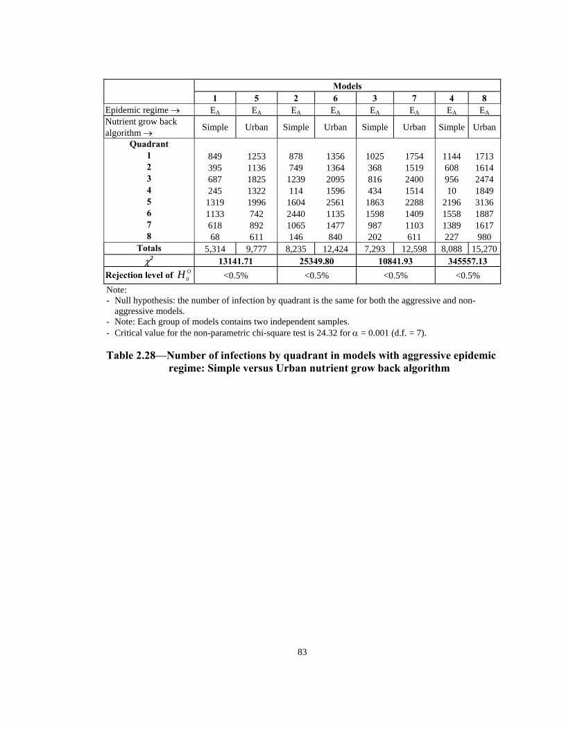
Models
1 5 2 6 3 7 4 8 Epidemic regime → EA EA EA EA EA EA EA EA
Nutrient grow back algorithm → Simple Urban Simple Urban Simple Urban Simple Urban
Quadrant 1 849 1253 878 1356 1025 1754 1144 1713 2 395 1136 749 1364 368 1519 608 1614 3 687 1825 1239 2095 816 2400 956 2474 4 245 1322 114 1596 434 1514 10 1849 5 1319 1996 1604 2561 1863 2288 2196 3136 6 1133 742 2440 1135 1598 1409 1558 1887 7 618 892 1065 1477 987 1103 1389 1617 8 68 611 146 840 202 611 227 980
Totals 5,314 9,777 8,235 12,424 7,293 12,598 8,088 15,270χ2 13141.71 25349.80 10841.93 345557.13
Rejection level of OH 0 <0.5% <0.5% <0.5% <0.5% Note: - Null hypothesis: the number of infection by quadrant is the same for both the aggressive and non-
aggressive models. - Note: Each group of models contains two independent samples. - Critical value for the non-parametric chi-square test is 24.32 for α = 0.001 (d.f. = 7). Table 2.28—Number of infections by quadrant in models with aggressive epidemic
regime: Simple versus Urban nutrient grow back algorithm
83
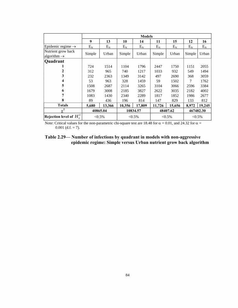
Models
9 13 10 14 11 15 12 16 Epidemic regime → EN EN EN EN EN EN EN EN
Nutrient grow back algorithm → Simple Urban Simple Urban Simple Urban Simple Urban
Quadrant 1 724 1514 1104 1796 2447 1750 1151 2055 2 312 965 740 1217 1033 932 549 1494 3 232 2363 1349 3142 497 2690 368 3059 4 53 963 328 1459 59 1502 7 1762 5 1508 2687 2114 3265 3104 3066 2596 3384 6 1679 3008 2185 3827 2622 3035 2182 4002 7 1083 1430 2340 2289 1817 1852 1986 2677 8 89 436 196 814 147 829 133 812
Totals 5,680 13,366 10,356 17,809 11,726 15,656 8,972 19,245χ2 40865.04 10834.57 48407.62 467482.30
R ejection level of OH <0.5% <0.5% <0.5% <0.5% 0
Note: Critical values for the non-parametric chi-square test are 18.48 for α = 0.01, and 24.32 for α = 0.001 (d.f. = 7).
Table 2.29— Number of infections by quadrant in models with non-aggressive
epidemic regime: Simple versus Urban nutrient grow back algorithm
84
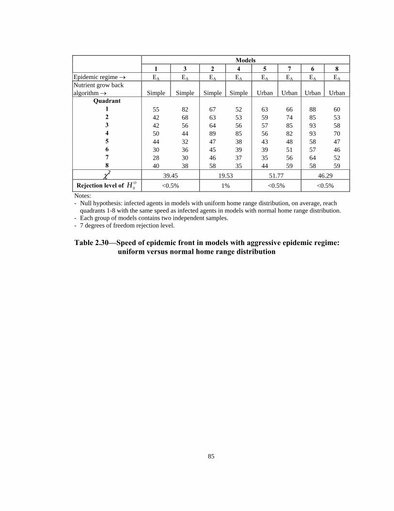
Models
1 3 2 4 5 7 6 8 Epidemic regime → EA EA EA EA EA EA EA EA
Nutrient grow back algorithm → Simple Simple Simple Simple Urban Urban Urban Urban
Quadrant 1 55 82 67 52 63 66 88 60 2 42 68 63 53 59 74 85 53 3 42 56 64 56 57 85 93 58 4 50 44 89 85 56 82 93 70 5 44 32 47 38 43 48 58 47 6 30 36 45 39 39 51 57 46 7 28 30 46 37 35 56 64 52 8 40 38 58 35 44 59 58 59 χ2 39.45 19.53 51.77 46.29
Rejection level of <0.5% 1% <0.5% <0.5% OH 0 Notes: - Null hypothesis: infected agents in models with uniform home range distribution, on average, reach
quadrants 1-8 with the same speed as infected agents in models with normal home range distribution. - Each group of models contains two independent samples. - 7 degrees of freedom rejection level. Table 2.30—Speed of epidemic front in models with aggressive epidemic regime:
uniform versus normal home range distribution
85
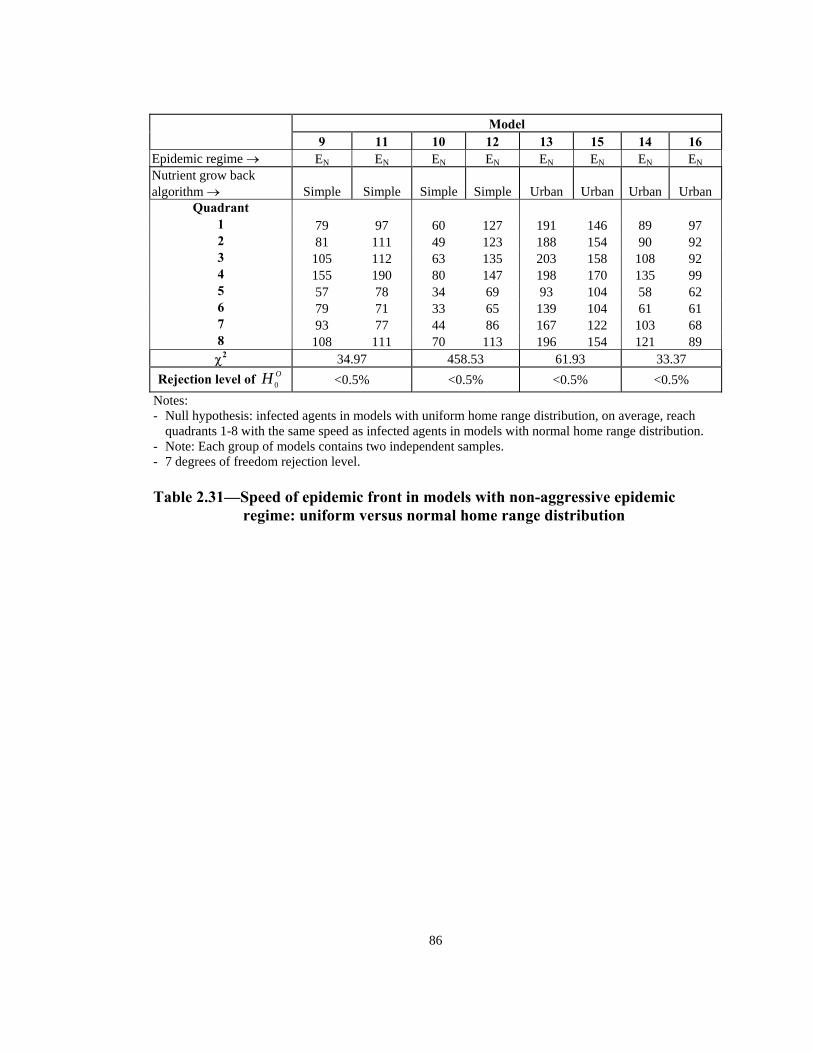
86
Model
9 11 10 12 13 15 14 16 Epidemic regime → EN EN EN EN EN EN EN EN
Nutrient grow back algorithm → Simple Simple Simple Simple Urban Urban Urban Urban
Quadrant 1 79 97 60 127 191 146 89 97 2 81 111 49 123 188 154 90 92 3 105 112 63 135 203 158 108 92 4 155 190 80 147 198 170 135 99 5 57 78 34 69 93 104 58 62 6 79 71 33 65 139 104 61 61 7 93 77 44 86 167 122 103 68 8 108 111 70 113 196 154 121 89 χ2 34.97 458.53 61.93 33.37
Rejection level of <0.5% <0.5% <0.5% <0.5% OH 0 Notes: - Null hypothesis: infected agents in models with uniform home range distribution, on average, reach
quadrants 1-8 with the same speed as infected agents in models with normal home range distribution. - Note: Each group of models contains two independent samples. - 7 degrees of freedom rejection level. Table 2.31—Speed of epidemic front in models with non-aggressive epidemic
regime: uniform versus normal home range distribution
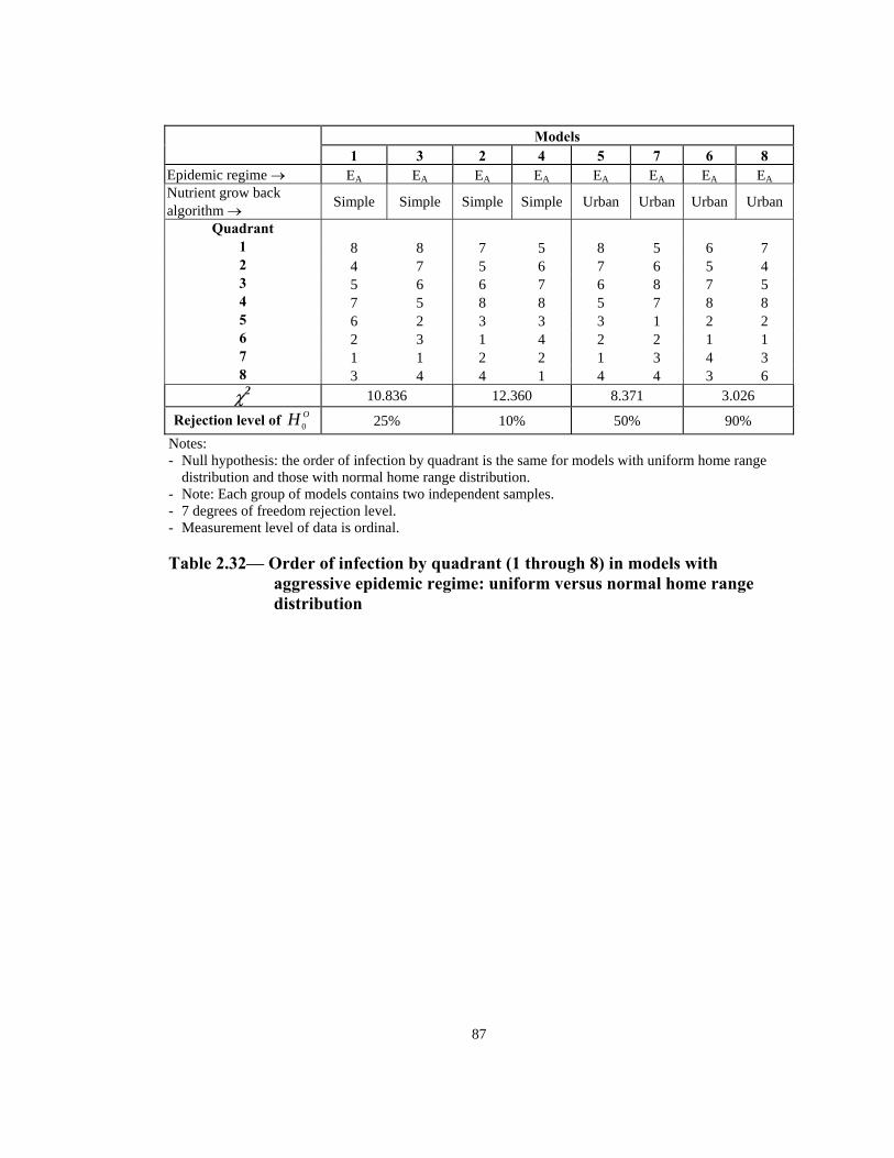
87
Models
1 3 2 4 5 7 6 8 Epidemic regime → EA EA EA EA EA EA EA EANutrient grow back algorithm → Simple Simple Simple Simple Urban Urban Urban Urban
Quadrant 1 8 8 7 5 8 5 6 7 2 4 7 5 6 7 6 5 4 3 5 6 6 7 6 8 7 5 4 7 5 8 8 5 7 8 8 5 6 2 3 3 3 1 2 2 6 2 3 1 4 2 2 1 1 7 1 1 2 2 1 3 4 3 8 3 4 4 1 4 4 3 6 χ2 10.836 12.360 8.371 3.026
Rejection level of OH 0 25% 10% 50% 90% Notes: - Null hypothesis: the order of infection by quadrant is the same for models with uniform home range
distribution and those with normal home range distribution. - Note: Each group of models contains two independent samples. - 7 degrees of freedom rejection level. - Measurement level of data is ordinal.
Table 2.32— Order of infection by quadrant (1 through 8) in models with
aggressive epidemic regime: uniform versus normal home range distribution
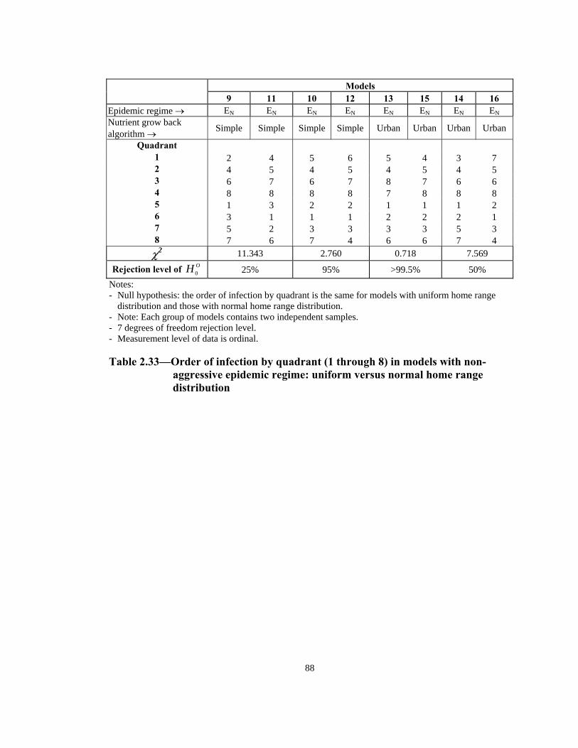
Models
9 11 10 12 13 15 14 16 Epidemic regime → EN EN EN EN EN EN EN EN
Nutrient grow back algorithm → Simple Simple Simple Simple Urban Urban Urban Urban
Quadrant 1 2 4 5 6 5 4 3 7 2 4 5 4 5 4 5 4 5 3 6 7 6 7 8 7 6 6 4 8 8 8 8 7 8 8 8 5 1 3 2 2 1 1 1 2 6 3 1 1 1 2 2 2 1 7 5 2 3 3 3 3 5 3 8 7 6 7 4 6 6 7 4 χ2 11.343 2.760 0.718 7.569
Rejection level of OH 0 25% 95% >99.5% 50% Notes: - Null hypothesis: the order of infection by quadrant is the same for models with uniform home range
distribution and those with normal home range distribution. wo independent samples. - Note: Each group of models contains t
- 7 degrees of freedom rejection level. - Measurement level of data is ordinal.
Table 2.33—Order of infection by quadrant (1 through 8) in models with non-
aggressive epidemic regime: uniform versus normal home range distribution
88
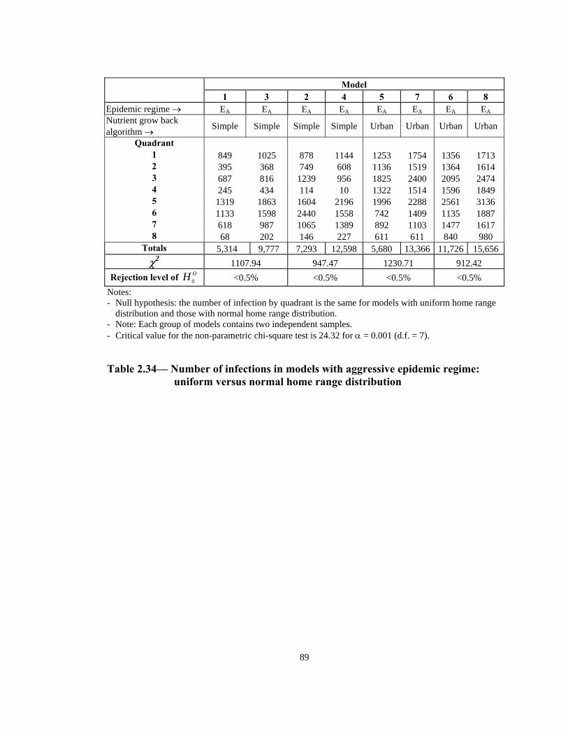
Model
1 3 2 4 5 7 6 8 Epidemic regime → EA EA EA EA EA EA EA EANutrient grow back algorithm → Simple Simple Simple Simple Urban Urban Urban Urban
Quadrant 1 849 1025 878 1144 1253 1754 1356 1713 2 395 368 749 608 1136 1519 1364 1614 3 687 816 1239 956 1825 2400 2095 2474 4 245 434 114 10 1322 1514 1596 1849 5 1319 1863 1604 2196 1996 2288 2561 3136 6 1133 1598 2440 1558 742 1409 1135 1887 7 618 987 1065 1389 892 1103 1477 1617 8 68 202 146 227 611 611 840 980
Totals 5,314 9,777 7,293 12,598 5,680 13,366 11,726 15,656 χ2 1107.94 947.47 1230.71 912.42
Rejection level of OH 0 <0.5% <0.5% <0.5% <0.5% Notes: - Null hypothesis: the number of infection by quadrant is the same for models with uniform home range
distribution and those with normal home range distribution. - Note: Each group of models contains two independent samples. - Critical value for the non-parametric chi-square test is 24.32 for α = 0.001 (d.f. = 7).
Table 2.34— Number of infections in models with aggressive epidemic regime: uniform versus normal home range distribution
89
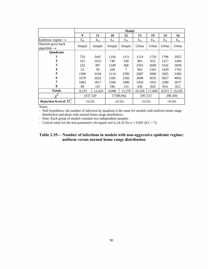
Model
9 11 10 12 13 15 14 16 Epidemic regime → EN EN EN EN EN EN EN ENNutrient grow back algorithm → Simple Simple Simple Simple Urban Urban Urban Urban
Quadrant 1 724 2447 1104 1151 1514 1750 1796 2055 2 312 1033 740 549 965 932 1217 1494 3 232 497 1349 368 2363 2690 3142 3059 4 53 59 328 7 963 1502 1459 1762 5 1508 3104 2114 2596 2687 3066 3265 3384 6 1679 2622 2185 2182 3008 3035 3827 4002 7 1083 1817 2340 1986 1430 1852 2289 2677 8 89 147 196 133 436 829 814 812
Totals 8,235 12,424 8,088 15,270 10,356 17,809 8,972 19,245 χ2 3337.520 17586.062 595.723 206.436
R <0.5% ejection level of OH 0 <0.5% <0.5% <0.5% Notes: - Null hypothesis: the number of infection by quadrant is the same for models with uniform home range
distribution and those with normal home range distribution. - Note: Each group of models contains two independent samples. -
Critical value for the non-parametric chi-square test is 24.32 for α = 0.001 (d.f. = 7).
Table 2.35— Number of infections in models with non-aggressive epidemic regime: uniform versus normal home range distribution
90
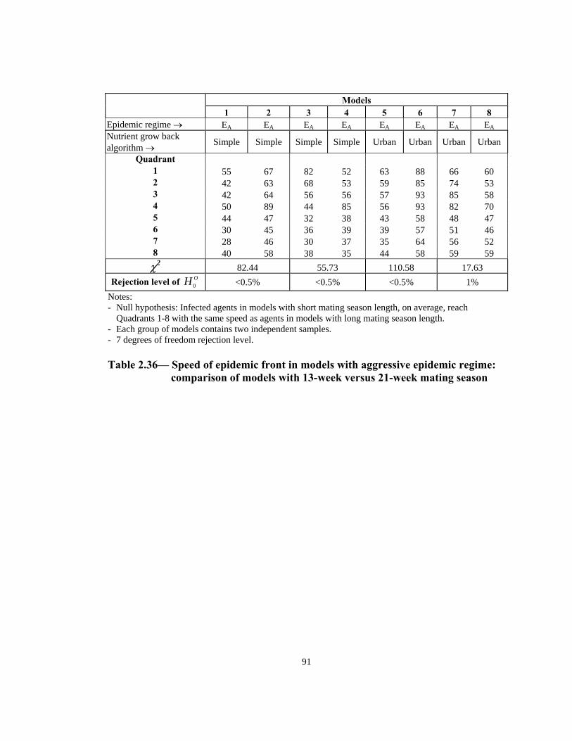
Models 1 2 3 4 5 6 7 8
Epidemic regime → EA EA EA EA EA EA EA EA
Nutrient grow back algorithm → Simple Simple Simple Simple Urban Urban Urban Urban
Quadrant 1 55 67 82 52 63 88 66 60 2 42 63 68 53 59 85 74 53 3 42 64 56 56 57 93 85 58 4 50 89 44 85 56 93 82 70 5 44 47 32 38 43 58 48 47 6 30 45 36 39 39 57 51 46 7 28 46 30 37 35 64 56 52 8 40 58 38 35 44 58 59 59 χ2 82.44 55.73 110.58 17.63
Rejection level of OH 0 <0.5% <0.5% <0.5% 1% Notes: - Null hypothesis: Infected agents in models with short mating season length, on average, reach
Quadrants 1-8 with the same speed as agents in models with long mating season length. - Each group of models contains two independent samples. - 7 degrees of freedom rejection level. Table 2.36— Speed of epidemic front in models with aggressive epidemic regime:
comparison of models with 13-week versus 21-week mating season
91
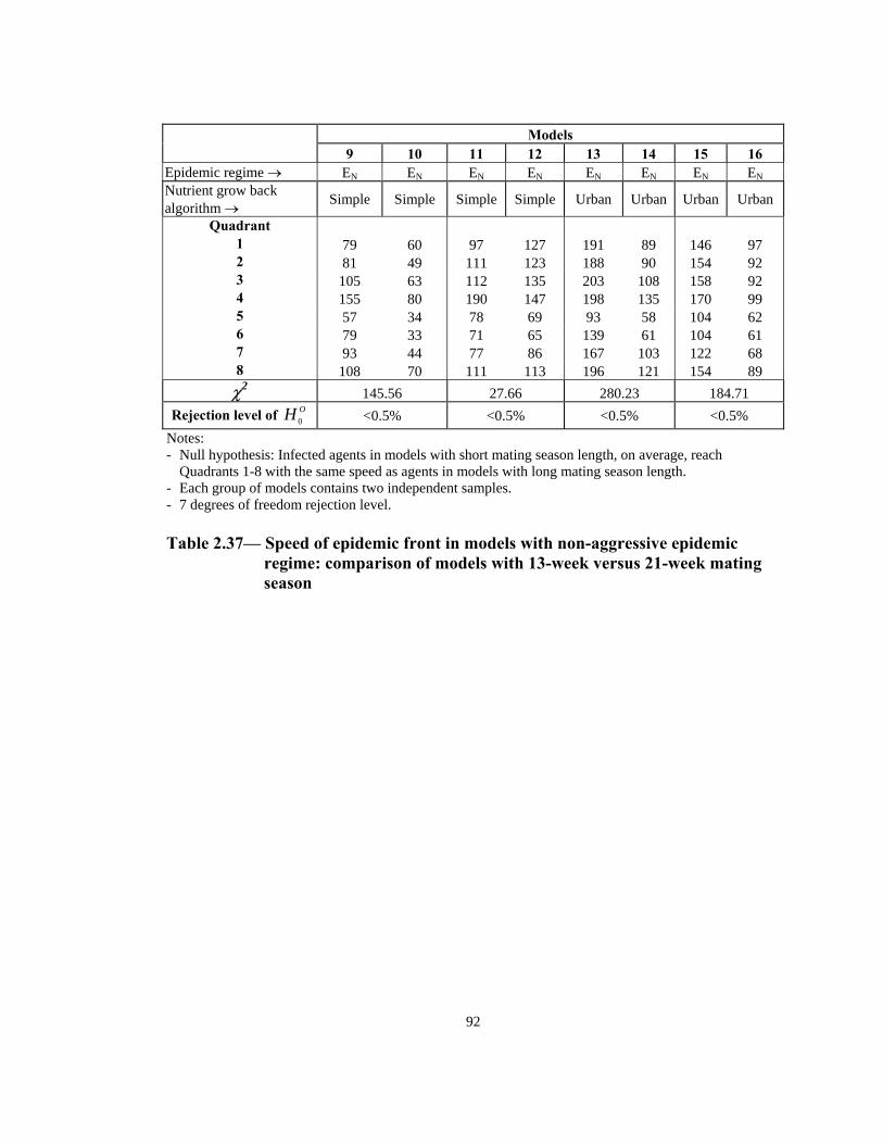
Models
9 10 11 12 13 14 15 16 Epidemic regime → EN EN EN EN EN EN EN EN
Nutrient grow back algorithm → Simple Simple Simple Simple Urban Urban Urban Urban
Quadrant 1 79 60 97 127 191 89 146 97 2 81 49 111 123 188 90 154 92 3 105 63 112 135 203 108 158 92 4 155 80 190 147 198 135 170 99 5 57 34 78 69 93 58 104 62 6 79 33 71 65 139 61 104 61 7 93 44 77 86 167 103 122 68 8 108 111 196 154 89 70 113 121 χ2 145.56 27.66 280.23 184.71
R <0.5% ejection level of OH 0 <0.5% <0.5% <0.5% Notes: - Null hypothesis: Infected agents in models with short mating season length, on average, reach
th long mating season length. Quadrants 1-8 with the same speed as agents in models widependent samples. - Each group of models contains two in
7 degrees of freedom rejection level. - Table 2.37— Speed of epidemic front in models with non-aggressive epidemic
regime: comparison of models with 13-week versus 21-week mating season
92
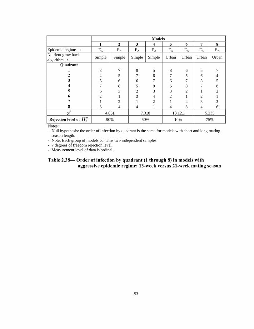
Models
1 2 3 4 6 7 8 5 Epidemic regime → EA EA EA EA EA EA EA EANutrient grow back algorithm → Simple Simple Simple Simple Urban Urban Urban Urban
Quadrant 1 8 7 8 5 8 6 5 7 2 4 5 7 6 7 5 6 4 3 5 6 6 7 6 7 8 5 4 7 8 5 8 5 8 7 8 5 6 3 2 3 3 2 1 2 6 2 1 3 4 2 1 2 1 7 4 1 2 1 2 1 3 3 8 3 4 1 3 6 4 4 4 χ2 4.051 7.318 13.121 5.235
Rejection level of OH 0 90% 50% 10% 75% Notes: - Null hypothesis: the order of infection by quadrant is the same for models with short and long mating
season length. - Note: Each group of models contains two independent samples. - 7 degrees of freedom rejection level. - Measurement level of data is ordinal.
Table 2.38— Order of infection by quadrant (1 through 8) in models with
aggressive epidemic regime: 13-week versus 21-week mating season
93

Models
9 10 11 12 14 15 13 16 Epidemic regime → EA EA EA EA EA EA EA EANutrient grow back algorithm → Simple Simple Simple Simple Urban Urban Urban Urban
Quadrant 1 2 5 4 6 5 3 4 7 2 4 4 5 5 4 4 5 5 3 6 6 7 7 8 6 7 6 4 8 8 8 8 7 8 8 8 5 1 2 3 2 1 1 1 2 6 3 1 1 1 2 2 2 1 7 5 3 2 3 3 5 3 3 8 7 7 7 6 4 6 6 4 χ2 7.633 2.943 2.500 4.560
R 50% 95% ejection level of OH 0 90% 75% Notes: - Null hypothesis: the order of infection by quadrant is the same for models with short and long mating
season length. wo independent samples. - Note: Each group of models contains t
- 7 degrees of freedom rejection level. - Measurement level of data is ordinal.
Table 2.39— Order of infection by quadrant (1 through 8) in models with non-
aggressive epidemic regime: 13-week versus 21-week mating season
94
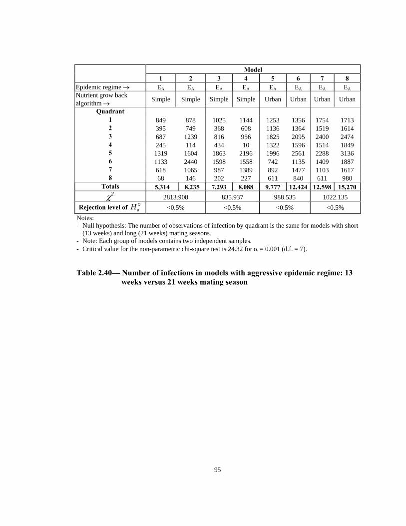
Model 1 2 3 4 5 6 7 8
Epidemic regime → EA EA EA EA EA EA EA EANutrient grow back algorithm → Simple Simple Simple Simple Urban Urban Urban Urban
Quadrant 1 849 878 1025 1144 1253 1356 1754 1713 2 395 749 368 608 1136 1364 1519 1614 3 687 1239 816 956 1825 2095 2400 2474 4 245 114 434 10 1322 1596 1514 1849 5 1319 1604 1863 2196 1996 2561 2288 3136 6 1133 2440 1598 1558 742 1135 1409 1887 7 618 1065 987 1389 892 1477 1103 1617 8 68 146 202 227 611 840 611 980
Totals 5,314 8,235 7,293 8,088 9,777 12,424 12,598 15,270 χ2 2813.908 835.937 988.535 1022.135
Rejection level of OH 0 <0.5% <0.5% <0.5% <0.5% Notes: - Null hypothesis: The number of observations of infection by quadrant is the same for models with short
(13 weeks) and long (21 weeks) mating seasons. - Note: Each group of models contains two independent samples. - Critical value for the non-parametric chi-square test is 24.32 for α = 0.001 (d.f. = 7).
Table 2.40— Number of infections in models with aggressive epidemic regime: 13 weeks versus 21 weeks mating season
95
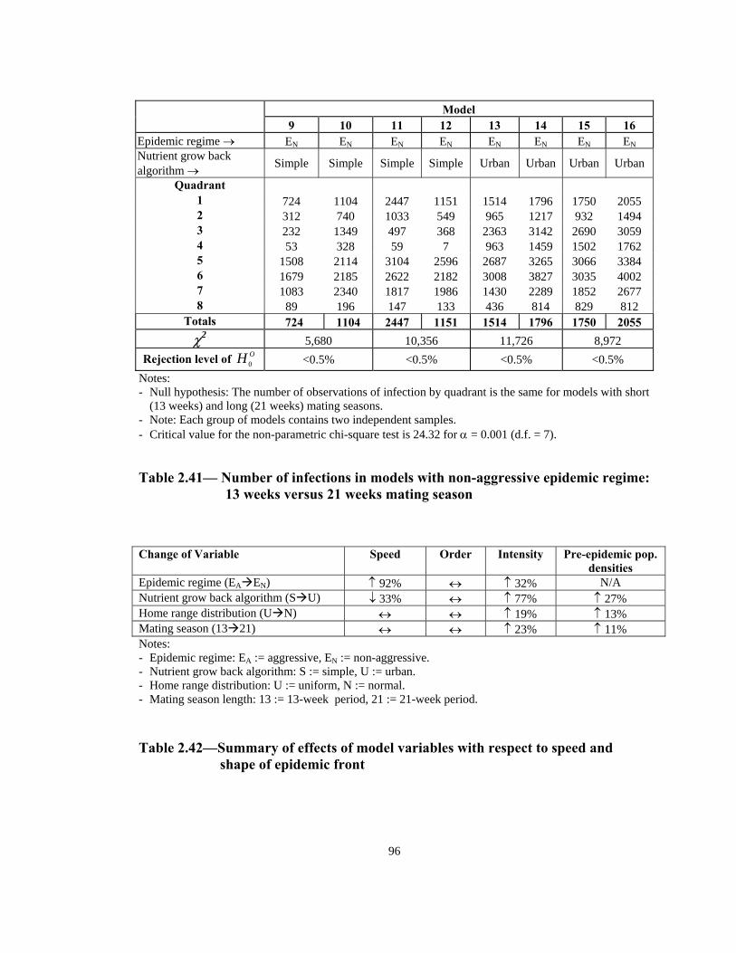
Model
9 10 11 12 13 14 15 16 Epidemic regime → EN EN EN EN EN EN EN ENNutrient grow back algorithm → Simple Simple Simple Simple Urban Urban Urban Urban
Quadrant 1 724 1104 2447 1151 1514 1796 1750 2055 2 312 740 1033 549 965 1217 932 1494 3 232 1349 497 368 2363 3142 2690 3059 4 53 328 59 7 963 1459 1502 1762 5 1508 2114 3104 2596 2687 3265 3066 3384 6 1679 2185 2622 2182 3008 3827 3035 4002 7 1083 2340 1817 1986 1430 2289 1852 2677 8 89 196 147 133 436 814 829 812
Totals 724 1104 2447 1151 1514 1796 1750 2055 χ2 5,680 10,356 11,726 8,972
Rejection level of OH 0 <0.5% <0.5% <0.5% <0.5% Notes: - Null hypothesis: The number of observations of infection by quadrant is the same for models with short
(13 weeks) and long (21 weeks) mating seasons. - Note: Each group of models contains two independent samples. Critical value for the non-parametric chi-square test is 24.32 for α = 0.001 (d.f. = 7). -
Table 2.41— Number of infections in models with non-aggressive epidemic regime: 13 weeks versus 21 weeks mating season
Change of Variable Speed Order Intensity Pre-epidemic pop.
densities Epidemic regime (EA EN) ↑ 92% ↔ ↑ 32% N/A Nutrient grow back algorithm (S U) ↓ 33% ↔ ↑ 77% ↑ 27% Home range distribution (U N) ↔ ↔ ↑ 19% ↑ 13% Mating season (13 21) ↔ ↔ ↑ 23% ↑ 11% Notes:
e. - Epidemic regime: EA := aggressive, EN := non-aggressiv- Nutrient grow back algorithm: S := simple, U := urban. - Home range distribution: U := uniform, N := normal. Mating season length: 13 := 13-week period, 21 := 21-week period. -
Table 2.42—Summary of effects of model variables with respect to speed and
shape of epidemic front
96
97
INTRODUCTION
In spite of the extensive research in modeling of outbreaks of terrestrial rabies, and
advances in vaccine development and methodologies for eradication of rabies from its
natural reservoirs, there are scant reports on systematic analysis of economic
consequences of rabies and its intervention.1 In this paper, I present results of agent-
based models that represent two different scenarios: one that simulates a raccoon rabies
epidemic outbreak and its potential economic cost in a hypothetical area where it has
previously been unaffected by raccoon rabies; the other that simulates the economic
cost of an effective ORV barrier that includes portions of the epidemic front and its
ARTICLE 3
Economic Analysis of a Raccoon Rabies Abatement Program: An Agent-Based Modeling Approach
OBJECTIVE
Develop a dynamic model that simulates the spread of raccoon rabies, and assess the
cost-effectiveness of orally administered rabies vaccine (ORV) as an intervention
method to abate raccoon rabies epidemic and its spread.
98
adjacent “rabies-free” area. The economic costs of these two scenarios, for different
ORV strategies, are compared to assess the economic viability of an ORV program.
MODELS
The models in this paper are a continuation of the models described in Article 2 which
consist of characterization of geographical areas by land use and its associated nutrient
growback rule ({Ē}), and agents by their genotype and behaviors ({Ā}) (see Article 2).
Results of simulations of two uninterrupted raccoon rabies epidemic scenarios
(aggressive epidemic: ({EC; G}, {AC; M, Mi, R, EA }) and non-aggressive epidemic:
({EC; G}, {AC; M, Mi, R, EN })) in a previously rabies-free area is compared to
alternative rabies abatement strategies (see Article 2). The alternative scenarios include
the enhancement of the environment with an ORV program (see below); hence, {Ē} is
modified to {EC; G, V}. Therefore, the characteristics and behavior of the model that
includes an ORV abatement strategy in compact form are denoted as ({Ē}, {Ā}) =
({EC; G, V}, {AC; M, Mi, R, E, C}).
METHODS
The technical specifications of the model are the same as those described in Article 2
with the exception of the ORV and rabies cost rules which are described below. Results
of the models are used to assess the cost-effectiveness of different ORV abatement
strategies compared to an uninterrupted raccoon rabies epidemic.
99
Space
The model’s space, a hypothetical 20-kilometer square space, is comprised of a lattice
of 100-m2 grids (total of 40,000 spatial units). The composition of the landscape is
designated as 20% urban, 20% wetland, 20% farmland, 15% forest, 15% prairie, 5%
water and 5% other (see Article 2). The model’s space is further divided into 16
quadrants (see Figure 3.1). Since the external initiation of disease is a random process
and may result in spurious results within the border quadrants, focus of the spread and
intensity of the epidemic is limited to the quadrants furthest away from the southern
border, Quadrants 1-8 (see Figure 3.1).
Agents
Initially, 8,000 agents are introduced to the model (20 agents/km2). For a duration of
500 periods, the agents move around in the model’s space, reproduce, die, and give rise
to their spatial distribution according to the land use categories (see Article 2). In
addition, agents move in and out of the model’s space through the migration rule (see
Article 2). At period 500 and every two periods thereafter, a rabid agent enters the
model’s space through its southern boundary. The point of entry for the rabid animal is
selected randomly, and each rabid animal can live up to a maximum of two weeks. Each
rabid agent that enters the model’s space lives for two periods. Rabid agents move
randomly within their home range (see Movement rule, Article 2) and infect susceptible
neighbors at their new position (non-aggressive epidemic regime). In the aggressive
epidemic regime, the rabid agent also infects all susceptible agents in its shortest path to
the new location (also see Epidemic rule, Article 2).
100
ORV rule, V
One method used to control and limit the spread of rabies is to vaccinate wildlife hosts
with ORV.2, 3 ORV is encased in baits and distributed over a designated area so that the
healthy susceptible portions of the population that serve as hosts will consume the
vaccine and bait and become protected against rabies infection. An effective ORV area
would stop the spread of rabies into geographical areas where raccoon rabies has not
been detected before. In the models presented here, the rate of bait placement serves as
a policy variable. The size of ORV barrier can also serve as a policy variable; however,
since the size of the model space in this paper is relatively small, this variable is not
tested. Other essential variables that determine the effectiveness of an ORV program
are the uptake of the vaccine baits by the target population and its effectiveness
(seroconversion rate). A sensitivity analyses is conducted around variables that are not
deemed certain: bait distribution and vaccine uptake (see Results), effectiveness of the
ORV, nutrient grow back algorithm of spatial units (see Article 2), and epidemic regime
(aggressive versus non-aggressive, see Article 2, and Table 3.1).
Vaccine uptake
Roscoe et al4 estimate that an ORV baiting (at a rate of 64 baits/km2) in a 552-km2 area
in New Jersey resulted in seroconversion of 61% of the sampled raccoons. Traces of
the vaccine were observed in 73% of raccoons in another sample in the same area. If
we assume that the proportion of vaccinated raccoons is a concave function of amount
of baits distributed per square kilometer, the range of this function would be from 0% of
101
raccoons vaccinated at zero amount of effort to nearly 100% at very high rate of bait
distribution. In this paper, a concave function of distribution rates is assumed with 70,
and 175 baits/km2 corresponding to vaccination rates of 65%, and 99%, respectively.
The simulations are conducted using different values of vaccination rates (see Figure
3.2). Accordingly, the additional cost of the increase in baits used is reflected in the
abatement cost.
Effectiveness
Rupprecht et al5 estimate that raccoons that ingested a form of ORV were protected
from rabies from 30 to 205 days from the time of ingestion. One of the vaccine
effectiveness regimes that is used in this paper is that when an agent becomes
vaccinated, it is protected against rabies between 5 and 30 weeks (U(5, 30)). Most
studies relating to the efficacy of ORV in raccoons have been conducted in laboratory
settings and may be much different in the field where variables such as herd immunity
also play a role in protection of the susceptible raccoons from rabies infection.
Therefore, a different range of rabies protection (U(30, 45)) is used in some of the
models to assess the sensitivity of results to the effectiveness of ORV. Figure 3.3 shows
the proportion of vaccinated susceptible agents through a duration of two years (four
ORV bait distributions at periods 500, 526, 552 and 578) with two different ORV
regimes. In one regime, the vaccination uptake by the susceptible animals is 65% and
the ORV effectiveness is distributed from a uniform distribution with a rnge of 5 to 30
weeks. The other regime, represents a superior ORV technology with is effectiveness
distributed from a uniform distribution with a range of 30 to 45 weeks and the ORV
102
effort results in successful vaccination of 99% of the susceptible agents within the ORV
barrier.
ORV algorithm
Figure 3.3 illustrates the implications of different assumptions on vaccine uptake and
effectiveness distribution. Hence, for an ORV strategy with 65% vaccine uptake and an
effectiveness distribution of U(5, 30), an average of 41.7% (minimum 8%) of the
susceptible agents in the ORV barrier are vaccinated during the two years depicted in
Figure 3.3. While the 99% vaccine uptake (effectiveness: U(30, 45)) strategy has an
average vaccination rate of 86% (minimum 61%).
ORV is typically distributed in an immune barrier that includes geographical areas that
cover portions of the raccoon rabies epidemic front and its adjacent “rabies-free” area.
Different rates of bait distribution (70, 100, 175 baits/km2), and effectiveness
distributions for a 10-kilometer wide ORV barrier is used to measure their cost-
effectiveness. The 10-kilometer ORV barrier includes quadrants 5-12 in the model’s
space (see Figure 3.4). At period 500, and every 26 periods thereafter, the ORV is
placed in the designated barrier. ORV baits are distributed at a cost of $23.23/km2 and
$1.47/bait (average of eight ORV distribution events in Ohio, see Article 1). Total cost
of ORV areas (V) and raccoon rabies cost (C) that spill into the ORV areas are then
computed for each period. The simulation ends at period 2600 (total of 50 years at 52
periods per year).
103
Rabies cost rule
Epidemic is defined as a period of time where there is a rapid increase in the level of
infection in an area. The epidemic period for raccoon rabies, in a medium-sized state,
typically lasts 3-4 years. The infection level eventually decreases as the number of
susceptible animals decreases whereby the infection enters the endemic stage. Due to
the frequency of rabies incidences, rabies cost in a region depends on whether rabies is
in its pre-epidemic (rabies free), epidemic, or endemic stage. A possible way of
mapping simulated rabies incidences to actual increase in rabies cost is to classify
whether a geographical entity, say a county, is in its pre-epidemic, epidemic or endemic
stage. The increase in raccoon rabies costs for epidemic and endemic areas, compared
to a base cost of a pre-epidemic year, is estimated in the form of $/km2 based on other
cost estimates for such areas cited from available literature (see below).
There has been sparse reporting on the cost of raccoon rabies. The most complete set of
cost estimates of raccoon rabies, presented by Uhaa et al (1992), indicates the cost of an
uninterrupted raccoon rabies epidemic in two counties in New Jersey (area: 2,137 km2)
in 1990 to be $1,011,844 ($474/km2).23 This estimate is based on the increase in
expenditure of human and animal health care, animal control, laboratory costs, rabies
education and research, and additional vaccination of pet animals from a pre-epizootic
year (1988) to an epizootic year (1990). Uhaa’s rabies cost estimate does not include
many elements such as value of avoided pain and suffering, or the public’s willingness
to pay to avoid the disease. Excluding the pet animal vaccinations, which are
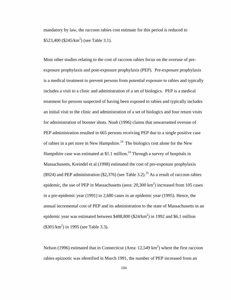
104
mandatory by law, the raccoon rabies cost estimate for this period is reduced to
$523,400 ($245/km2) (see Table 3.1).
Most other studies relating to the cost of raccoon rabies focus on the overuse of pre-
exposure prophylaxis and post-exposure prophylaxis (PEP). Pre-exposure prophylaxis
is a medical treatment to prevent persons from potential exposure to rabies and typically
includes a visit to a clinic and administration of a set of biologics. PEP is a medical
treatment for persons suspected of having been exposed to rabies and typically includes
an initial visit to the clinic and administration of a set of biologics and four return visits
for administration of booster shots. Noah (1996) claims that unwarranted overuse of
PEP administration resulted in 665 persons receiving PEP due to a single positive case
of rabies in a pet store in New Hampshire.24 The biologics cost alone for the New
Hampshire case was estimated at $1.1 million.24 Through a survey of hospitals in
Massachusetts, Kreindel et al (1998) estimated the cost of pre-exposure prophylaxis
($924) and PEP administration ($2,376) (see Table 3.2).25 As a result of raccoon rabies
epidemic, the use of PEP in Massachusetts (area: 20,300 km2) increased from 105 cases
in a pre-epidemic year (1991) to 2,680 cases in an epidemic year (1995). Hence, the
annual incremental cost of PEP and its administration to the state of Massachusetts in an
epidemic year was estimated between $488,800 ($24/km2) in 1992 and $6.1 million
($301/km2) in 1995 (see Table 3.3).
Nelson (1996) estimated that in Connecticut (Area: 12,549 km2) where the first raccoon
rabies epizootic was identified in March 1991, the number of PEP increased from an
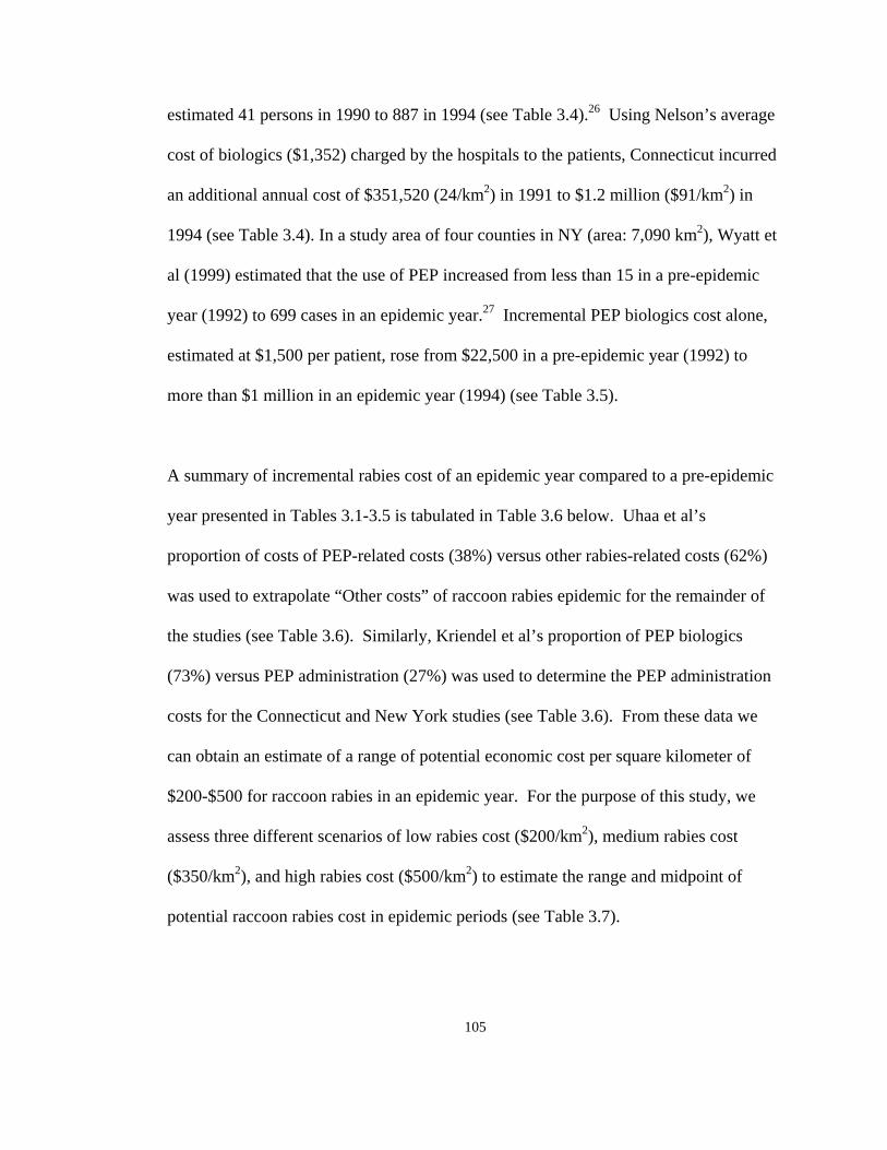
105
estimated 41 persons in 1990 to 887 in 1994 (see Table 3.4).26 Using Nelson’s average
cost of biologics ($1,352) charged by the hospitals to the patients, Connecticut incurred
an additional annual cost of $351,520 (24/km2) in 1991 to $1.2 million ($91/km2) in
1994 (see Table 3.4). In a study area of four counties in NY (area: 7,090 km2), Wyatt et
al (1999) estimated that the use of PEP increased from less than 15 in a pre-epidemic
year (1992) to 699 cases in an epidemic year.27 Incremental PEP biologics cost alone,
estimated at $1,500 per patient, rose from $22,500 in a pre-epidemic year (1992) to
more than $1 million in an epidemic year (1994) (see Table 3.5).
A summary of incremental rabies cost of an epidemic year compared to a pre-epidemic
year presented in Tables 3.1-3.5 is tabulated in Table 3.6 below. Uhaa et al’s
proportion of costs of PEP-related costs (38%) versus other rabies-related costs (62%)
was used to extrapolate “Other costs” of raccoon rabies epidemic for the remainder of
the studies (see Table 3.6). Similarly, Kriendel et al’s proportion of PEP biologics
(73%) versus PEP administration (27%) was used to determine the PEP administration
costs for the Connecticut and New York studies (see Table 3.6). From these data we
can obtain an estimate of a range of potential economic cost per square kilometer of
$200-$500 for raccoon rabies in an epidemic year. For the purpose of this study, we
assess three different scenarios of low rabies cost ($200/km2), medium rabies cost
($350/km2), and high rabies cost ($500/km2) to estimate the range and midpoint of
potential raccoon rabies cost in epidemic periods (see Table 3.7).

106
Kemere et al (1999) estimates on the economic impact of raccoon rabies were based on
population of affected geographic areas ($/100,000 population).28 Excluding the pet
animal vaccination costs, these estimates were distinguished by incremental cost
(compared to pre-epidemic year) of epidemic year ($87,800/100,000) and endemic year
($51,700/100,000). Although one cannot readily compare these hypothetical cost
figures ($/population) with those in Tables 3.1-3.6 ($/km2), it can be said that rabies
cost for endemic years, according to Kemere et al, is roughly 60% of an epidemic year
(see Table 3.7).
The proxy costs presented in Table 3.7 is used to map the level of rabies activity in a
specified area (based on quadrants in models in this paper) to its cost.
RESULTS
To demonstrate the methodology of systematically calculating cost of an uninterrupted
raccoon rabies event and the cost of potential alternative ORV distribution strategies,
three models are selected from Article 2: Models 1, 5 and 16 (see Table 3.8). Results
from Article 2 indicate that Model 1 has the fastest moving epidemic front with rabies
reaching Quadrants 1-8 in an average of 42 weeks (see Table 3.9 and also Article 2).
The amounts of time it takes for the rabies epidemic to reach Quadrants 1-8 in Models 5
and 16, on average, are 50 and 83 weeks, respectively. Article 2 also indicates that, in
an uninterrupted rabies epidemic event, in Quadrants 1-8, Model 16 results in the
largest number if infections (19,245) (see Table 3.10). In contrast, between the 16
models simulated in Article 2, in Quadrants 1-8, Model 1 produced the least number of
infections (5,314) while Model 5 produced 9,777 infections (see Table 3.10). For each
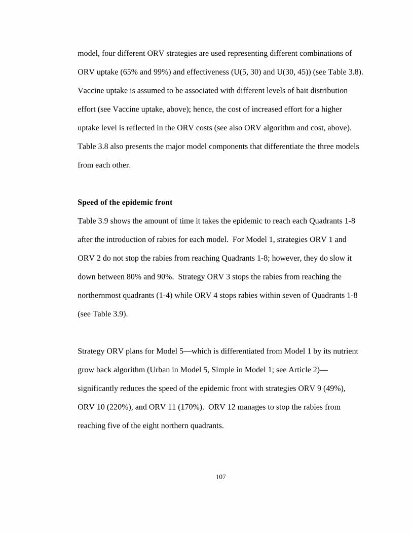
107
model, four different ORV strategies are used representing different combinations of
ORV uptake (65% and 99%) and effectiveness (U(5, 30) and U(30, 45)) (see Table 3.8).
Vaccine uptake is assumed to be associated with different levels of bait distribution
effort (see Vaccine uptake, above); hence, the cost of increased effort for a higher
uptake level is reflected in the ORV costs (see also ORV algorithm and cost, above).
Table 3.8 also presents the major model components that differentiate the three models
from each other.
Speed of the epidemic front
Table 3.9 shows the amount of time it takes the epidemic to reach each Quadrants 1-8
after the introduction of rabies for each model. For Model 1, strategies ORV 1 and
ORV 2 do not stop the rabies from reaching Quadrants 1-8; however, they do slow it
down between 80% and 90%. Strategy ORV 3 stops the rabies from reaching the
northernmost quadrants (1-4) while ORV 4 stops rabies within seven of Quadrants 1-8
(see Table 3.9).
Strategy ORV plans for Model 5—which is differentiated from Model 1 by its nutrient
grow back algorithm (Urban in Model 5, Simple in Model 1; see Article 2)—
significantly reduces the speed of the epidemic front with strategies ORV 9 (49%),
ORV 10 (220%), and ORV 11 (170%). ORV 12 manages to stop the rabies from
reaching five of the eight northern quadrants.
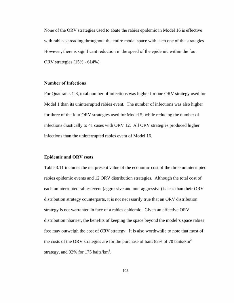
108
Epidemic and ORV costs
Table 3.11 includes the net present value of the economic cost of the three uninterrupted
rabies epidemic events and 12 ORV distribution strategies. Although the total cost of
each uninterrupted rabies event (aggressive and non-aggressive) is less than their ORV
distribution strategy counterparts, it is not necessarily true that an ORV distribution
strategy is not warranted in face of a rabies epidemic. Given an effective ORV
distribution nbarrier, the benefits of keeping the space beyond the model’s space rabies
free may outweigh the cost of ORV strategy. It is also worthwhile to note that most of
the costs of the ORV strategies are for the purchase of bait: 82% of 70 baits/km2
strategy, and 92% for 175 baits/km2.
None of the ORV strategies used to abate the rabies epidemic in Model 16 is effective
with rabies spreading throughout the entire model space with each one of the strategies.
However, there is significant reduction in the speed of the epidemic within the four
ORV strategies (15% - 614%).
Number of Infections
For Quadrants 1-8, total number of infections was higher for one ORV strategy used for
Model 1 than its uninterrupted rabies event. The number of infections was also higher
for three of the four ORV strategies used for Model 5; while reducing the number of
infections drastically to 41 cases with ORV 12. All ORV strategies produced higher
infections than the uninterrupted rabies event of Model 16.
109
DISCUSSION
In this paper, three models that represent three separate simulation of raccoon rabies
epidemic in a hypothetical area are selected from Article 2. For each model, four
different ORV strategies are implemented in separate simulations to compare the effect
of each ORV strategy on the speed of epidemic and number of infections with that of
the uninterrupted counterpart model. The four different ORV strategies consist of
different combination of ORV distribution effort, and assumed effectiveness of the
ORVs. Not all ORV strategies proved to be effective in that the disease still moved
across the ORV barrier in to the area that was supposed to be protected by it; however,
overall, the rate of movement was greatly diminished. For three ORV distribution
strategies, where effectiveness of the ORV was assumed to last between 30 and 45 days,
the ORV barrier proved to be effective. One of these scenarios assumed ORV uptake of
65% by the susceptible population in the ORV barrier, while the other two scenarios
assumed 99% uptake. These results underscore the need for improvement in ORV
technology.
There were mixed results on the number of infections in each model before and after
implementation of an ORV distribution strategy. In Model 1, the number of infections
increased under an ORV distribution strategy in one of four cases, while in Models 5
and 16 in three and four out of four cases, respectively, the number of infections rose
after implementation of an ORV distribution strategy. Although it seems
counterintuitive that implementation of an ORV distribution strategy would actually

110
The benefit cost ratios indicate that given the coverage of the model’s space (400 km2),
implementation of an ORV distribution strategy is not economically justifiable.
However, the benefits derived from an effective ORV distribution strategy by far
extends beyond the adjacent areas of the ORV barrier. For example, in a westward
movement of raccoon rabies, an effective ORV distribution strategy in the state of Ohio
would benefit all states west of Ohio. These benefits would be realized in the form
foregone medical costs and epidemic outbreak program costs borne by the local, state
and federal agencies. Moreover, this analysis does not take into account potential loss
of wildlife, pet animals, livestock, psychological trauma to humans or their willingness
to pay for abatement of raccoon rabies spread.
increase the number of rabies cases, it seems that this peculiar result is a byproduct of
the relatively small model space and the edge effect created by the influx of susceptible
migrant agents into the model. In the uninterrupted rabies simulations, after the
epidemic front sweeps throughout the model, the model’s space initially gets populated
around the edges and eventually agents move to the middle of model’s space. Under
the ORV strategies, the vaccinated agents in the middle portion of the model’s space
continue to reproduce and therefore extend a larger susceptible and unprotected agent
population than an uninterrupted rabies event. It is also possible that the reproduction
rule and/or spatial characteristics and grow back rule (see Article 2) are not realistic and
results in the overpopulation of the model’s space.
111
Rabies in wildlife is typically a regional and persistent health problem; therefore, the
economic costs and benefits of an ORV program should be considered over a broad
region and over a long period. Collaboration among different regions could result in
several economies of scale, such as reduced price of ORV from the purchase of large
quantities of baits. Regional cooperation could also lead to economies of scale by
hiring new personnel and purchasing new equipment and material; in existing ORV
programs, both are currently contracted out to external agencies (eg, fixed-wing aircraft,
pilots, etc.). Hence, in order to assess the economic viability of an ORV strategy in face
of raccoon rabies epidemic, different policies in regards to the procurement of materials
and personnel need to be considered.
The information presented here can be refined with additional knowledge on raccoon
ecology and epidemiologic characteristics of rabies in raccoons to predict future spread
of rabies as well as the economic impact of using ORV. Several scenarios may need to
be evaluated, and they will be important in determining the feasibility of regional and
national efforts and in designing future interventions to control this public health
problem.
112
REFERENCES: ARTICLE 3
1. Meltzer MI, Rupprecht CE. A review of the economics of the prevention and
control of rabies,” Pharmacoeconomics 1998; 14:365-383.
2. Winkler WG, Jenkins SR. Raccoon rabies. In: Baer GM, ed. The natural history of
rabies. 2nd ed. Boca Raton, Fla.: CRC Press Inc, 1991; 1991:325-340.
3. Rupprecht CE, Wiktor TJ, Johnston DH, et al. Oral immunization and protection of
raccoons (Procyon lotor) with a vaccinia-rabies glycoprotein recombinant virus
vaccine. Proc Natl Acad Sci U S A 1986; 83:7947-7950.
4. Roscoe DE, Holste WC, Sorhage FE, Campbell C et al. Efficacy of an oral vaccinia-
rabies glycoprotein recombinant vaccine in controlling epidemic raccoon rabies in
New Jersey. J Wildl Dis. 1998 Oct; 34(4):752-63.
5. Rupprecht CE, Hamir AN, Johnston DH, Koprowski H. Efficacy of a vaccinia-
rabies glycoprotein recombinant virus vaccine in raccoons (Procyon lotor). Rev
Infect Dis. 1988 Nov-Dec; 10 Suppl 4:S803-9.
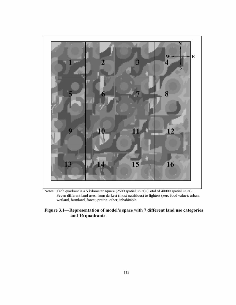
Notes: Each quadrant is a 5 kilometer square (2500 spatial units) (Total of 40000 spatial units).
1 2 3 4
5 6 7 8
9 10 11 12
13 14 15 16
N
W
S
E
Seven different land uses, from darkest (most nutritious) to lightest (zero food value): urban, wetland, farmland, forest, prairie, other, inhabitable.
Figure 3.1—Representation of model’s space with 7 different land use categories
and 16 quadrants
113
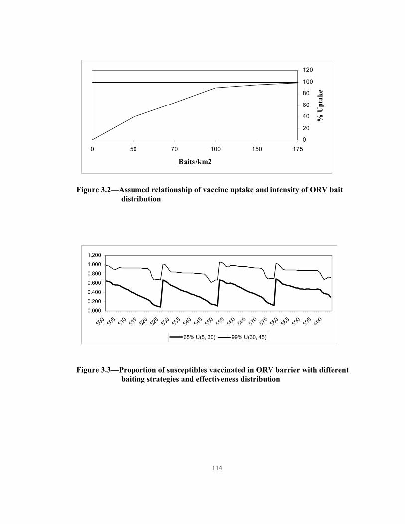
0
20
40
60
80
100
120
0 50 70 100 150 175
Baits/km2
% U
ptak
e
Figure 3.2—Assumed relationship of vaccine uptake and intensity of ORV bait
distribution
0.000
0.200
0.400
0.600
0.800
1.000
1.200
500
505
510
515
520
525
530
535
540
545
550
555
560
565
570
575
580
585
590
595
600
65% U(5, 30) 99% U(30, 45)
Figure 3.3—Proportion of susceptibles vaccinated in ORV barrier with different
baiting strategies and effectiveness distribution
114
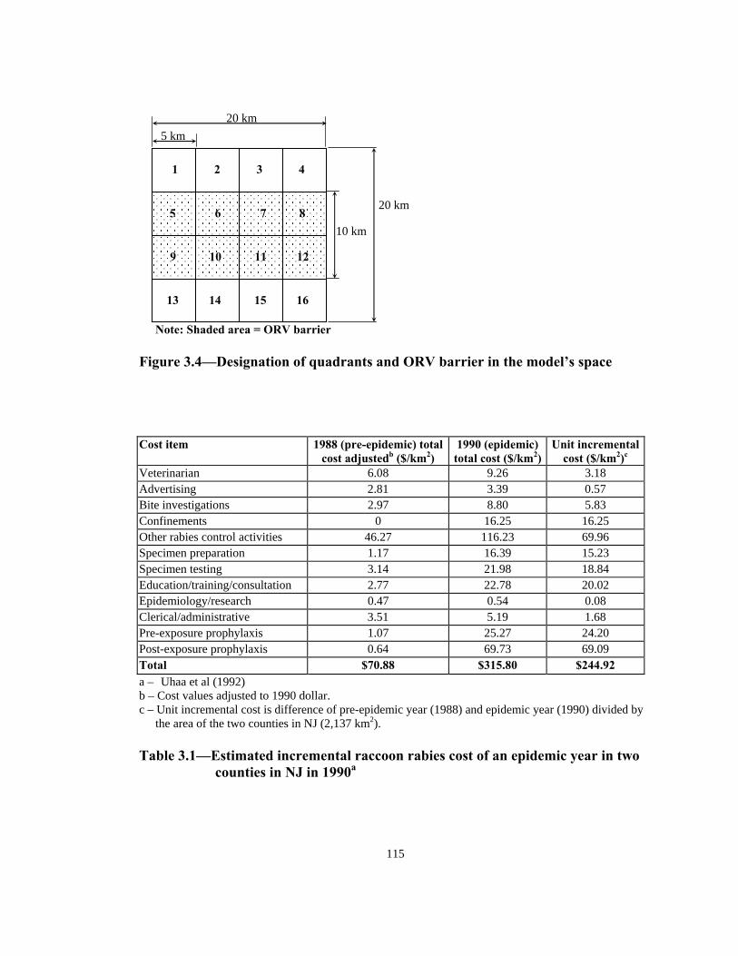
Note: Shaded area = ORV barrier
5 km 20 km
5 6 7 8
9 10 11 12
13 14 15 16
1 2 3 4
10 km
20 km
Figure 3.4—Designation of quadrants and ORV barrier in the model’s space
115
Cost item 1988 (pre-epidemic) total cost adjustedb ($/km2)
1990 (epidemic) total cost ($/km2)
Unit incrementalcost ($/km2)c
Veterinarian 6.08 9.26 3.18 Advertising 2.81 3.39 0.57 Bite investigations 2.97 8.80 5.83 Confinements 0 16.25 16.25 Other rabies control activities 46.27 116.23 69.96 Specimen preparation 1.17 16.39 15.23 Specimen testing 3.14 21.98 18.84 Education/training/consultation 2.77 22.78 20.02 Epidemiology/research 0.47 0.54 0.08 Clerical/administrative 3.51 5.19 1.68 Pre-exposure prophylaxis 1.07 25.27 24.20 Post-exposure prophylaxis 0.64 69.73 69.09 Total $70.88 $315.80 $244.92 a – Uhaa et al (1992) b – Cost values adjusted to 1990 dollar. c – Unit incremental cost is difference of pre-epidemic year (1988) and epidemic year (1990) divided by
the area of the two counties in NJ (2,137 km2). Table 3.1—Estimated incremental raccoon rabies cost of an epidemic year in two
counties in NJ in 1990a
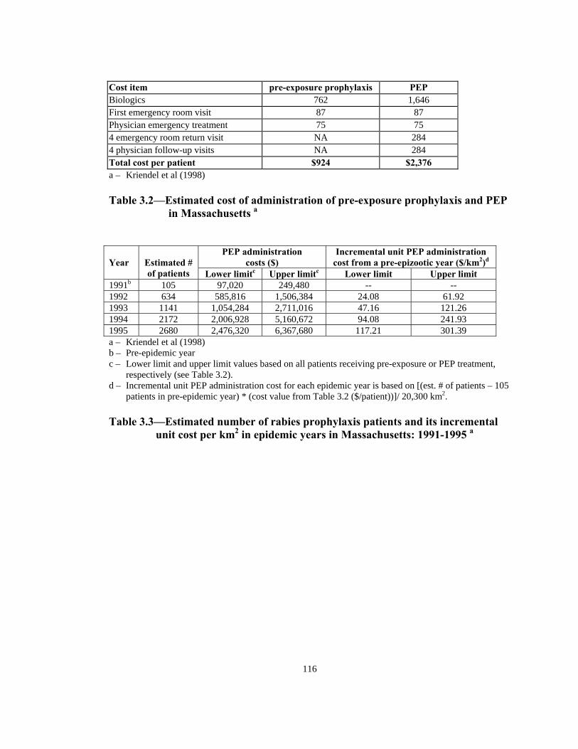
116
Cost item pre-exposure prophylaxis PEP Biologics 762 1,646 First emergency room visit 87 87 Physician emergency treatment 75 75 4 emergency room return visit NA 284 4 physician follow-up visits NA 284 Total cost per patient $924 $2,376 a – Kriendel et al (1998) Table 3.2—Estimated cost of administration of pre-exposure prophylaxis and PEP
in Massachusetts a
costs ($) Incremental unit PEP administration
cost from a pre-epizootic year ($/km2)d
PEP administration Year
Estimated # of patients Lower limitc Upper limitc Lower limit Upper limit
1991b 105 97,020 249,480 -- -- 1992 634 585,816 1,506,384 24.08 61.92 1993 1141 1,054,284 2,711,016 47.16 121.26 1994 2172 2,006,928 5,160,672 94.08 241.93 1995 2680 2,476,320 6,367,680 117.21 301.39 a – Kriendel et al (1998) b – Pre-epidemic year c – Lower limit and upper limit values based on all patients receiving pre-exposure or PEP treatment,
respectively (see Table 3.2). d – Incremental unit PEP administration cost for each epidemic year is based on [(est. # of patients – 105
patients in pre-epidemic year) * (cost value from Table 3.2 ($/patient))]/ 20,300 km2. Table 3.3—Estimated number of rabies prophylaxis patients and its incremental
unit cost per km2 in epidemic years in Massachusetts: 1991-1995 a
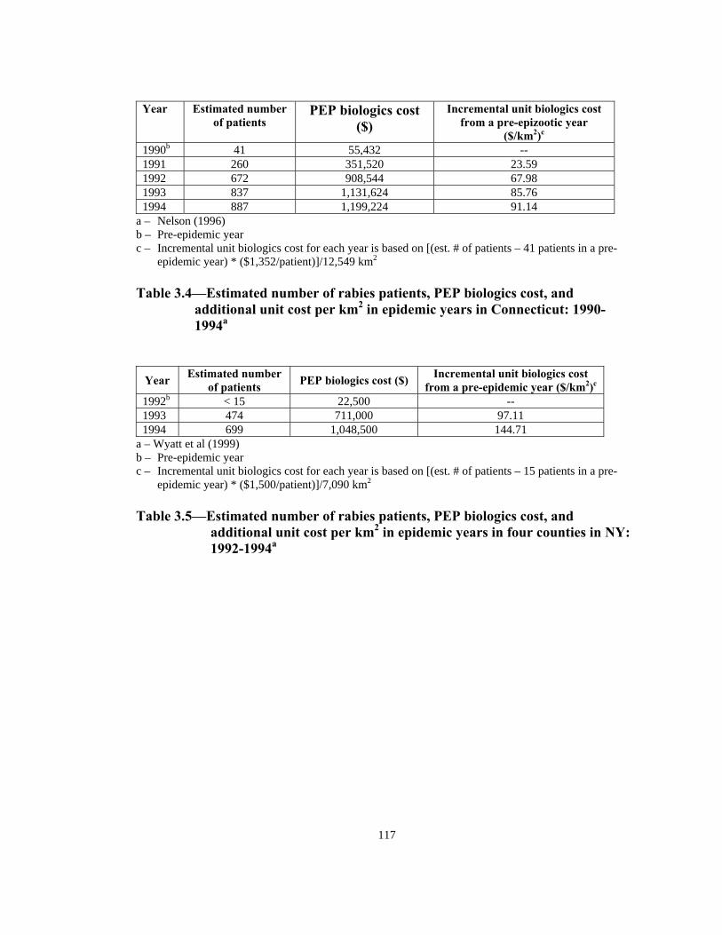
117
PEP biologics cost ($)
Incremental unit biologics cost from a pre-epizootic year
($/km2)c
Year Estimated number
of patients
1990b 55,432 41 -- 1991 260 351,520 23.59 1992 672 908,544 67.98 1993 837 1,131,624 85.76 1994 887 1,199,224 91.14
a – Nelson (1996) b – Pre-epidemic year c – Incremental unit biologics cost for each year is based on [(est. # of patients – 41 patients in a pre-
epidemic year) * ($1,352/patient)]/12,549 km2
Table 3.4—Estimated number of rabies patients, PEP biologics cost, and additional unit cost per km2 in epidemic years in Connecticut: 1990-1994a
Year PEP biologics cost ($) Incremental unit biologics cost from a pre-epidemic year ($/km2)c
Estimated number of patients
1992b < 15 22,500 -- 1993 474 711,000 97.11 1994 699 1,048,500 144.71
a – Wyatt et al (1999) b – Pre-epidemic year c – Incremental unit biologics cost for each year is based on [(est. # of patients – 15 patients in a pre-
epidemic year) * ($1,500/patient)]/7,090 km2
Table 3.5—Estimated number of rabies patients, PEP biologics cost, and
additional unit cost per km2 in epidemic years in four counties in NY: 1992-1994a
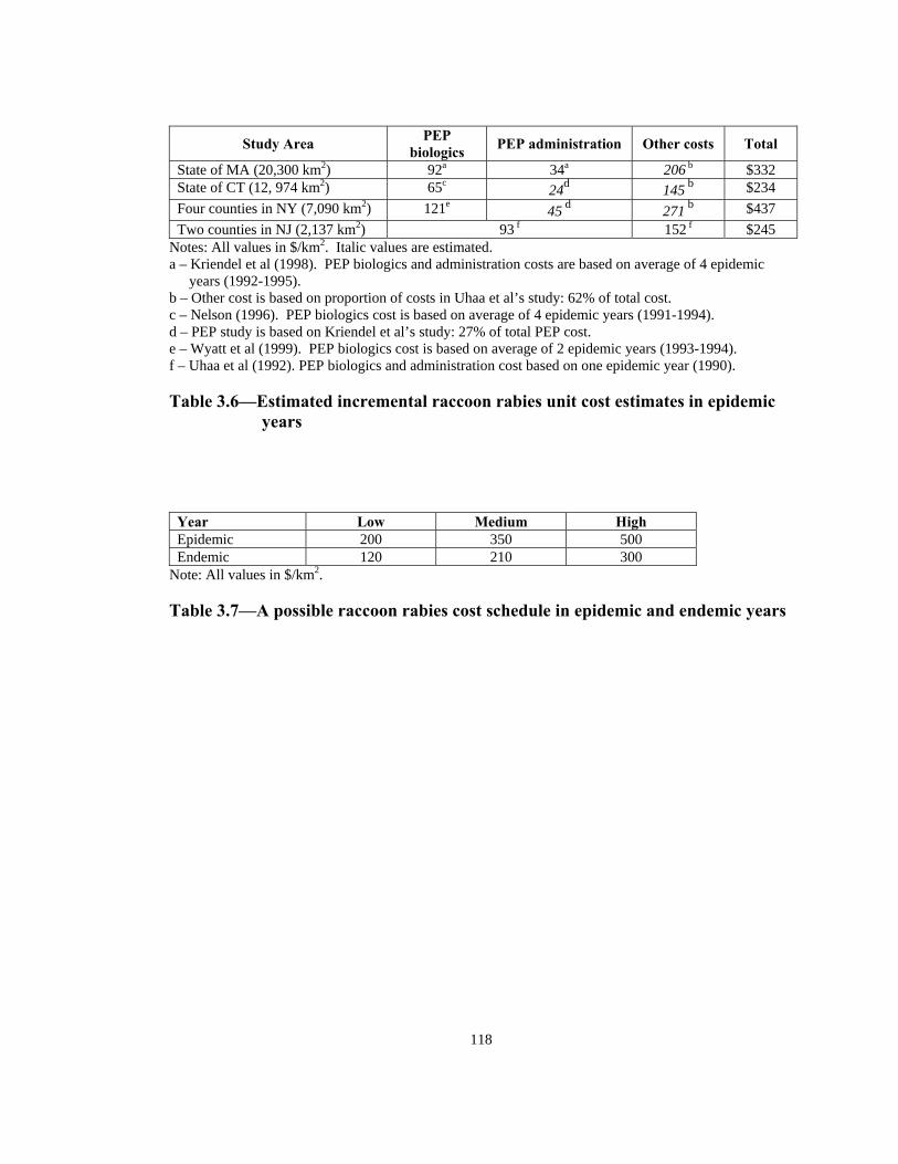
118
PEP administration
Study Area PEP
biologics Other costs Total
State of MA (20,300 km2) 92a 34a 206 b $332 State of CT (12, 974 km2) 65c 24d 145 b $234 Four counties in NY (7,090 km2) 121e 45 d 271 b $437 Two counties in NJ (2,137 km2) 93 f 152 f $245
Notes: All values in $/km2. Italic values are estimated.
High
a – Kriendel et al (1998). PEP biologics and administration costs are based on average of 4 epidemic years (1992-1995).
b – Other cost is based on proportion of costs in Uhaa et al’s study: 62% of total cost. c – Nelson (1996). PEP biologics cost is based on average of 4 epidemic years (1991-1994). d – PEP study is based on Kriendel et al’s study: 27% of total PEP cost. e – Wyatt et al (1999). PEP biologics cost is based on average of 2 epidemic years (1993-1994). f – Uhaa et al (1992). PEP biologics and administration cost based on one epidemic year (1990). Table 3.6—Estimated incremental raccoon rabies unit cost estimates in epidemic
years
Year Low Medium Epidemic 200 350 500 Endemic 120 210 300
Note: All values in $/km2. Table 3.7—A possible raccoon rabies cost schedule in epidemic and endemic years
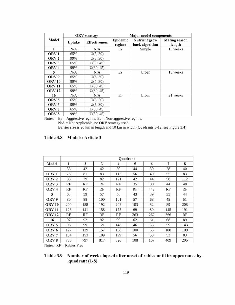
119
ORV strategy Major model components
Model Uptake Effectiveness Epidemic regime
Nutrient grow back algorithm
Mating season length
1 N/A N/A ORV 1 65% U(5, 30) ORV 2 99% U(5, 30) ORV 3 65% U(30, 45) ORV 4 99% U(30, 45)
EA Simple 13 weeks
5 N/A N/A ORV 9 65% U(5, 30)
ORV 10 99% U(5, 30) ORV 11 65% U(30, 45) ORV 12 99% U(30, 45)
EA Urban 13 weeks
16 N/A N/A ORV 5 65% U(5, 30) ORV 6 99% U(5, 30) ORV 7 65% U(30, 45) ORV 8 99% U(30, 45)
EN Urban 21 weeks
Notes: E = Aggressive regime, E = Non-aggressive regime. A NN/A = Not Applicable, no ORV strategy used.
Barrier size is 20 km in length and 10 km in width (Quadrants 5-12, see Figure 3.4). Table 3.8—Models: Article 3 Quadrant
Model 1 2 3 4 5 6 7 8 1 55 42 42 50 44 30 28 40
ORV 1 75 81 83 115 56 49 55 83 ORV 2 88 79 82 121 42 44 58 112 ORV 3 RF RF RF RF 30 44 35 48 ORV 4 RF RF RF RF RF 449 RF RF
5 63 59 57 56 43 39 35 44 ORV 9 80 88 100 101 57 68 45 51
ORV 10 200 188 192 208 103 82 89 208 ORV 11 126 141 158 175 69 89 145 191 ORV 12 RF RF RF RF 263 262 366 RF
16 97 92 92 99 62 61 68 89 ORV 5 96 99 121 148 46 53 59 143 ORV 6 127 139 157 168 100 65 108 109 ORV 7 154 153 189 199 56 53 53 83 ORV 8 785 797 817 826 108 107 409 205
Notes: RF = Rabies Free Table 3.9—Number of weeks lapsed after onset of rabies until its appearance by
quadrant (1-8)

120
Quadrant
Model 1 2 3 4 5 6 7 8 Total 1 849 395 687 245 1319 1133 618 68 5,314
ORV 1 969 410 243 63 1394 705 260 45 4,089 ORV 2 903 930 2177 583 583 286 164 40 5,666 ORV 3 0 0 0 0 26 44 7 1 78 ORV 4 0 0 0 0 0 1 0 0 1
5 1253 1136 1825 1322 1996 742 892 611 9,777 ORV 9 1226 906 1590 1329 1952 1478 1131 596 10,208
ORV 10 1510 1558 1981 1444 2016 1916 952 313 11,690 ORV 11 2315 1623 2627 1870 2937 2334 1357 427 15,490 ORV 12 0 0 0 0 15 24 2 0 41
16 2055 1494 3059 1762 3384 4002 2677 812 19,245 ORV 5 3229 4547 2681 2254 4383 3344 1496 536 22,470 ORV 6 4174 1721 998 8864 4168 8849 2861 351 31,986 ORV 7 5957 3363 7766 2354 3851 1952 1021 304 26,568 ORV 8 4589 25,669 3731 11638 2987 1288 657 594 185
Table 3.10—Number of infections by quadrant (1-8)
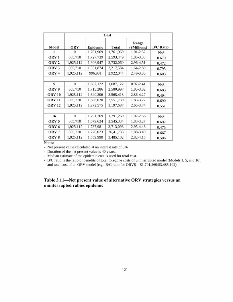
121
Cost
Model ORV Epidemic Total Range
($Millions) B/C Ratio
1 0 1,761,969 1,761,969 1.01-2.52 N/A ORV 1 865,710 1,727,739 2,593,449 1.85-3.33 0.679 ORV 2 1,925,112 1,806,947 3,732,060 2.96-4.51 0.472 ORV 3 865,710 1,351,874 1.64-2.80 2,217,584 0.795 ORV 4 1,925,112 0.603 996,931 2,922,044 2.49-3.35
5 1,687,122 0 1,687,122 0.97-2.41 N/A
ORV 9 865,710 1,715,286 2,580,997 1.85-3.32 0.683 ORV 10 1,925,112 1,640,306 3,565,418 2.86-4.27 0.494 ORV 11 865,710 1,686,020 2,551,730 1.83-3.27 0.690 ORV 12 1,925,112 1,272,575 3,197,687 2.65-3.74 0.551
16 0 1,791,269 1,791,269 1.02-2.56 N/A
ORV 5 865,710 1,679,624 2,545,334 1.83-3.27 0.692 ORV 6 1,925,112 1,787,981 3,713,093 2.95-4.48 0.475 ORV 7 865,710 1,776,023 26,41,733 1.88-3.40 0.667 ORV 8 1,559,990 2.82-4.15 1,925,112 3,485,102 0.506
Notes: - Net present value calculated at an interest rate of 5%. - Duration of the net present value is 40 years. - Median estimate of the epidemic cost is used for total cost. - B/C ratio is the ratio of benefits of total foregone costs of uninterrupted model (Models 1, 5, and 16)
and total cost of an ORV model (e.g., B/C ratio for ORV8 = $1,791,269/$3,485,102) Table 3.11—Net present value of alternative ORV strategies versus an uninterrupted rabies epidemic
122
2. Kreindel SM, McGuill M, Meltzer M, et al. The cost of rabies postexposure prophylaxis: One state’s experience. Public Health Rep 1998; 13:247-251.
BIBLIOGRAPHY
1. Uhaa LJ, Dato VM, Sorhage FE, et al. Benefits and costs of using an orally
absorbed vaccine to control rabies in raccoons. J Am Vet Med Assoc 1992; 201:1873-1882.
3. Robbins AH, Borden MD, Windmiller BS, et al. Prevention of the spread of rabies
to wildlife by oral rabies vaccination of raccoons in Massachusetts. J Am Vet Med Assoc 1998; 213:1407-1412.
4. Winkler WG, Jenkins SR. Raccoon rabies. In: Baer GM, ed. The natural history of
rabies. 2nd ed. Boca Raton, FL: CRC Press Inc.; 1991:325-340. 5. Fischman HR, Grigor JK, Horman JT, et al. Epizootic of rabies in raccoons in
Maryland from 1981 to 1987. J Am Vet Med Assoc 1992; 201:1883-1886. 6. Torrence ME, Jenkins SR, Glickman LT. Epidemology of raccoon rabies in
Virginia, 1984 to 1989. J Wildl Dis 1992; 28:369-376. 7. Krebs JW, Rupprecht CE, Childs JE. Rabies surveillance in the United States
during 1999. J Am Vet Med Assoc 2000; 217:1799-1811. 8. Smith KA. Update on rabies in Ohio. Ohio Vet Med Assoc Newslett 1998; 29:5.
9. Wandeler A, Rosatte RC, Williams D, et al. Update: Raccoon rabies epizootic -
United States and Canada, 1999. MMWR Morb Mortal Wkly Rep 2000; 49:31-35. 10. Aubert, MFA. Costs and benefits of rabies control in wildlife in France. Rev sci
tech 1999; 18:533-543.
123
11. Nelson RS, Cooper GH, Cartter ML, et al. Rabies postexposure prohylaxis—
Connecticut, 1990-1994. MMWR Morb Mortal Wkly Rep 1996; 45:232-234. 12. Rupprecht CE, Wiktor TJ, Johnston DH, et al. Oral immunization and protection of
raccoons (Procyon lotor) with a vaccinia-rabies glycoprotein recombinant virus vaccine. Proc Natl Acad Sci U S A 1986; 83:7947-7950.
13. Anderson RM, Jackson HC, May RM, et al. Population dynamics of fox rabies in
Europe. Nature 1981; 289:765-771. 14. Wandeler AI. Oral immunization of wildlife. In: Baer GM, ed. The natural history
of rabies. 2nd ed. Boca Raton, FL: CRC Press Inc., 1991; 485-503. 15. Fearneyhough MG, Wilson PJ, Clark KA, et al. Results of an oral rabies
vaccination program for coyotes. J Am Vet Med Assoc 1998; 212:498-502. 16. Meltzer MI, Rupprecht CE. A review of the economics of the prevention and
control of rabies,” Pharmacoeconomics 1998; 14:365-383. 17. Meltzer, MI. Assessing the costs and benefits of an oral vaccine for raccoon rabies:
a possible model. Emerg Infect Dis 1996; 2:336-342. 18. Kermack WO, McKendrick AG. A contribution to the mathematical theory of
epidemics. Proc. R. Soc. 1927; A115:700-721. 19. Anderson RM, Jackson HC, May RM, et al. Population Dynamics of Fox Rabies in
Europe. Nature 1981; 289:765-771. 20. Holmes EE, Lewis MA, Banks JE, et al. Partial differential equations in ecology:
spatial interactions and population dynamics. Ecology 1994; 75(1):17-29. 21. Smith ADM. A continuous time deterministic model of temporal rabies. In:
Bacon, PJ ed. Population dynamics of rabies in wildlife. Orlando, Fla: Academic Press Inc, 1985; 131-145.

124
22. Artois M, Langlais M, Suppo C. Simulation of rabies control within an increasing
fox population. Ecological Modelling 1997; 23-34. 23. Müller J. Optimal vaccination patterns in age-structured populations: endemic case.
Mathematical and Computer Modelling 2000; 31:149-160. 24. Iannelli M, Kim MY, Park EJ. Splitting methods for the numerical approximation
of some models of age-structured population dynamics and epidemiology. Applied Mathematics and Computation 1997; 87:69-93.
25. Garnerin P, Hazout S, Valleron AJ. Estimation of two epidemiological parameters of fox rabies: the length of incubation period and the dispersion distance of cubs. Ecological Modelling 1986; 33:123-135.
26. Smith DL, Lucey B, Waller LA, et al. Predicting the spatial dynamics of rabies
epidemics on heterogeneous landscapes. Proc. Natl. Acad. Sci. 2002; 99(6)3668:3672.
27. Maasilta P. Forecasting the HIV epidemic in Finland by using functional small area
units. GeoJournal 1997; 41.3:215-222.
28. Anderson J. Providing a broad spectrum of agents in spatially explicit simulation models: the Gensim approach. In: Gimblett HR ed. Integrating geographic information systems and agent-based modeling techniques. New York, NY: Oxford University Press, 2002; 21:58.
29. Gimblett HR. Integrating geographic information systems and agent-based
technologies for modeling and simulating social and ecological phenomena. In: Gimblett HR ed. Integrating geographic information systems and agent-based modeling techniques. New York, NY: Oxford University Press, 2002; 1:20.
30. Epstein JM, Axtell R. Growing artificial societies. Washington DC: Brookings
Institution Press, 1996.
125
31. Lotze AH. In: Chapman JA, Feldhamer GA, eds. Wild mammals of North America. Baltimore: The Johns Hopkins University Press, 1982; 586-597.
32. Kaufmann JH. Raccoon and allies. In: Chapman JA, Feldhamer GA, eds. Wild
mammals of North America. Baltimore: The Johns Hopkins University Press, 1982; 567-585.
33. Wilson DE, Ruff S. The Smithsonian book of North American mammals.
Washington DC: Smithsonian Institution Press, 1999; 221-223. 34. Merritt JF. Guide to the mammals of Pennsylvania. Matinko RA, ed. Pittsburgh,
PA: University of Pittsburgh Press, 1987; 266-269. 35. Whitaker JO, Hamilton WJ, eds. Mammals of the eastern United States. Third
edition. Ithaca, NY: Comstock Publishing Associates, 1998; 427-433. 36. Stuewer FE. Raccoons: their habits and management in Michigan. Ecological
Monographs, 13(2):205-256. 37. Sanderson GC, Nalbandov AV. The reproductive cycle of the raccoon in Illinois.
Illinois Natural History Survey Bulletin 1973. 31(2):29-84. 38. Nowak RM. Walker’s mammals of the world. Fifth Ed, Vol. II.. The Johns
Hopkins University Press, 1991; 1100-1101. 39. Winkler WG, Jenkins SR. Raccoon rabies. In: Baer GM, ed. The natural history of
rabies. 2nd ed. Boca Raton, Fla.: CRC Press Inc, 1991; 1991:325-340. 40. Uhaa IJ, Dato VM, Sorhage FE, et al. Benefits and costs of using an orally
absorbed vaccine to control rabies in raccoons. JAVMA, 201(12):1873-1882, 1992. 41. Noah DL, Smith MG, Gotthardt JC, et al. Mass human exposure to rabies in New
Hampshire: exposures, treatment, and cost.
126
42. Kreindel SM, McGuill M, Meltzer M, et al. The cost of rabies postexposure prophylaxis: one state’s experience. Public Health Reports, 113:247-251, 1998.
43. Nelson RS, Cooper GH, Cartter ML, et al. Rabies postexposure prophylaxis –
Connecticut, 1990-1994. MMWR, 45(11):232-234, 1996. 44. Wyatt JD, Barker WH, Bennett NM, et al. Human rabies postexposure prophylaxis
during a raccoon rabies epizootic in New York, 1993 and 1994. Emerging Infectious Diseases 1999, 5(3):415-423.
45. Kemere P, Liddel MK, Evangelou P, et al. Economic analysis of a large scale oral
vaccination program to control raccoon rabies. Unpublished Report, 1999. 46. Meltzer MI, Rupprecht CE. A review of the economics of the prevention and
control of rabies,” Pharmacoeconomics 1998; 14:365-383. 47. Winkler WG, Jenkins SR. Raccoon rabies. In: Baer GM, ed. The natural history of
rabies. 2nd ed. Boca Raton, Fla.: CRC Press Inc, 1991; 1991:325-340. 48. Rupprecht CE, Wiktor TJ, Johnston DH, et al. Oral immunization and protection of
raccoons (Procyon lotor) with a vaccinia-rabies glycoprotein recombinant virus vaccine. Proc Natl Acad Sci U S A 1986; 83:7947-7950.
49. Roscoe DE, Holste WC, Sorhage FE, Campbell C et al. Efficacy of an oral vaccinia-
rabies glycoprotein recombinant vaccine in controlling epidemic raccoon rabies in New Jersey. J Wildl Dis. 1998 Oct; 34(4):752-63.
50. Rupprecht CE, Hamir AN, Johnston DH, Koprowski H. Efficacy of a vaccinia-
rabies glycoprotein recombinant virus vaccine in raccoons (Procyon lotor). Rev Infect Dis. 1988 Nov-Dec; 10 Suppl 4:S803-9.
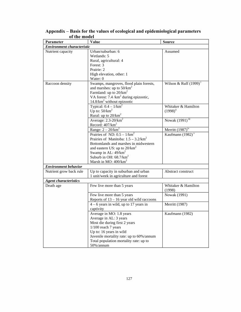
127
Appendix – Basis for the values of ecological and epidemiological parameters of the model Parameter Value Source Environment characteristic Nutrient capacity Urban/suburban: 6
Wetlands: 5 Rural, agricultural: 4 Forest: 3 Prairie: 2 High elevation, other: 1 Water: 0
Assumed
Swamps, mangroves, flood plain forests, and marshes: up to 50/km2
Farmland: up to 20/km2
VA forest: 7.4 /km2 during epizootic, 14.8/km2 without epizootic
Wilson & Ruff (1999) i
Typical: 0.4 – 1/km2
Up to: 50/km2
Rural: up to 20/km2
Whitaker & Hamilton (1998)ii
Average: 2.3-20/km2
Record: 407/km2Nowak (1991) iii
Range: 2 – 20/km2 Merritt (1987)iv
Raccoon density
Prairies of ND: 0.5 – 1/km2
Prairies of Manitoba: 1.5 – 3.2/km2
Bottomlands and marshes in midwestern and eastern US: up to 20/km2
Swamp in AL: 49/km2
Suburb in OH: 68.7/km2
Marsh in MO: 400/km2
Kaufmann (1982) v
Environment behavior Nutrient grow back rule Up to capacity in suburban and urban
1 unit/week in agriculture and forest Abstract construct
Agent characteristics Few live more than 5 years Whitaker & Hamilton
(1998) Few live more than 5 years Reports of 13 – 16 year old wild raccoons
Nowak (1991)
4 – 6 years in wild, up to 17 years in captivity
Merritt (1987)
Death age
Average in MO: 1.8 years Average in AL: 3 years Most die during first 2 years 1/100 reach 7 years Up to: 16 years in wild Juvenile mortality rate: up to 60%/annum Total population mortality rate: up to 50%/annum
Kaufmann (1982)

128
Appendix continued Parameter Value Source Agent characteristics continued Fat reserve Varies. Random endowment +
accumulated food/period – metabolism/period
Assumed
1 – 5 units Assumed Metabolism 0.32 cc O2/g hr Kaufmann (1982)
Agent behavior: movement rule Travel 0.75-2.5 km/night Wilson & Ruff (1999)
Juvenile: moved 264 km Whitaker & Hamilton (1998)
Movement
Maximum: 11.2 km/night MN juvenile: 1.7 km/week in 156 weeks Manitoba juvenile: 10.8/week in 23 weeks
Kaufmann (1982)
Males: 0.65 km2
Females: 0.39 km2
Range: 0.002-49.6 km2
Nowak (1991)
Typical: 8 km2/year Range: 0.5 – 50 km2/year
Macdonald (1989)vi
Range: 0.05 – 50 km2/year Merritt (1987)
Home range
Maximum: 0.79 km2 – 7.07 km2 Suburban: 0.07 km2 – 0.38 km2 Prairies in ND: : 78.54 km2 Typical: 0.4 - 1 km2
Kaufmann (1982)
Agent behavior: migration rule Migration 52% of raccoons immigrated to previously
epizootic area Wilson & Ruff (1999)
Agent behavior: reproduction rule Feb-Jun, Peak: Mar Wilson & Ruff (1999) Dec-Aug, Peaks: Feb-Mar Nowak (1991) Late Jan – early Feb Can also mate into summer
Macdonald (1989)
Typical: Jan – Feb Merritt (1987) Northern limit: Feb-Jun, Peak: March Entire North America: Jan-Mar Peak: Feb GA, LA, SC: most in Mar AL: Mar – Jun, Peak: Apr FL: year-round, most in Dec – Aug
Kaufmann (1982)
Mating season
Feb-Mar Stuewer (1943)vii
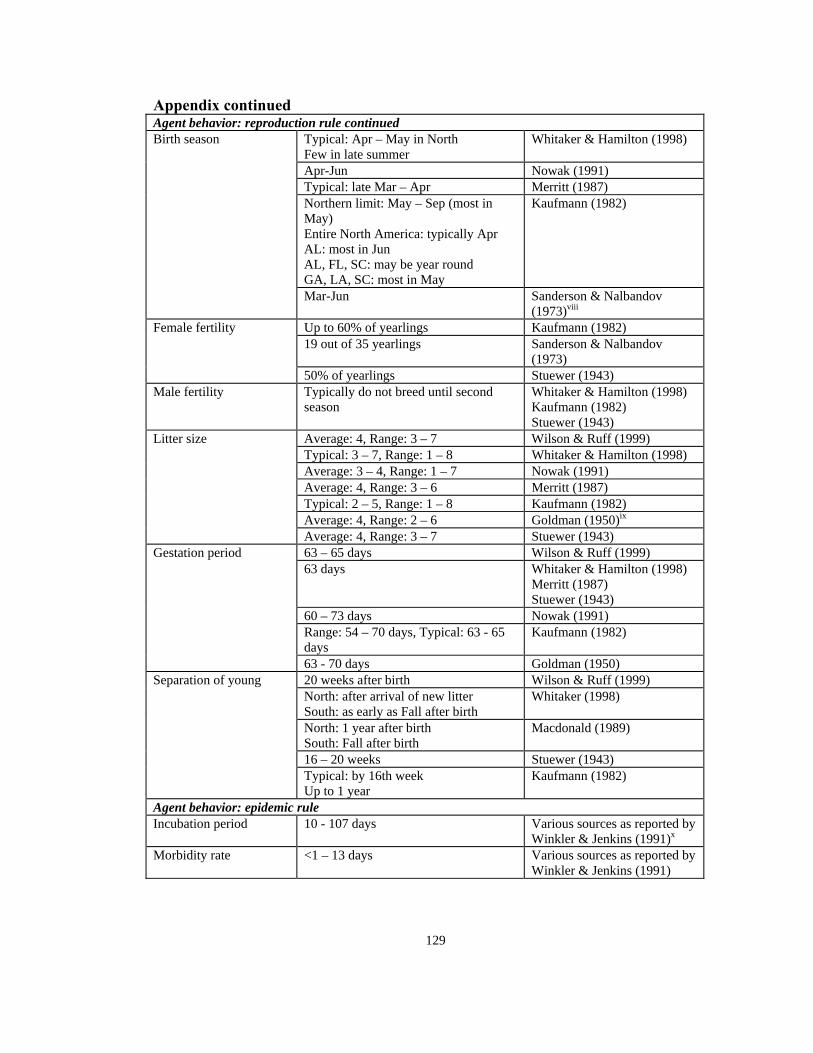
129
Appendix continued Agent behavior: reproduction rule continued
Typical: Apr – May in North Few in late summer
Whitaker & Hamilton (1998)
Apr-Jun Nowak (1991) Typical: late Mar – Apr Merritt (1987) Northern limit: May – Sep (most in May) Entire North America: typically Apr AL: most in Jun AL, FL, SC: may be year round GA, LA, SC: most in May
Kaufmann (1982)
Birth season
Mar-Jun Sanderson & Nalbandov (1973)viii
Up to 60% of yearlings Kaufmann (1982) 19 out of 35 yearlings Sanderson & Nalbandov
(1973)
Female fertility
50% of yearlings Stuewer (1943) Male fertility Typically do not breed until second
season Whitaker & Hamilton (1998) Kaufmann (1982) Stuewer (1943)
Average: 4, Range: 3 – 7 Wilson & Ruff (1999) Typical: 3 – 7, Range: 1 – 8 Whitaker & Hamilton (1998) Average: 3 – 4, Range: 1 – 7 Nowak (1991) Average: 4, Range: 3 – 6 Merritt (1987) Typical: 2 – 5, Range: 1 – 8 Kaufmann (1982) Average: 4, Range: 2 – 6 Goldman (1950)ix
Litter size
Average: 4, Range: 3 – 7 Stuewer (1943) 63 – 65 days Wilson & Ruff (1999) 63 days Whitaker & Hamilton (1998)
Merritt (1987) Stuewer (1943)
60 – 73 days Nowak (1991) Range: 54 – 70 days, Typical: 63 - 65 days
Kaufmann (1982)
Gestation period
63 - 70 days Goldman (1950) 20 weeks after birth Wilson & Ruff (1999) North: after arrival of new litter South: as early as Fall after birth
Whitaker (1998)
North: 1 year after birth South: Fall after birth
Macdonald (1989)
16 – 20 weeks Stuewer (1943)
Separation of young
Typical: by 16th week Up to 1 year
Kaufmann (1982)
Agent behavior: epidemic rule Incubation period 10 - 107 days Various sources as reported by
Winkler & Jenkins (1991)x
Morbidity rate <1 – 13 days Various sources as reported by Winkler & Jenkins (1991)
130
i Wilson DE, Ruff S. The Smithsonian book of North American mammals. Washington DC: Smithsonian Institution Press, 1999; 221-223. ii Whitaker JO, Hamilton WJ, eds. Mammals of the eastern United States. Third edition. Ithaca, NY: Comstock Publishing Associates, 1998; 427-433. iii Nowak, RM. Walker’s mammals of the world. 5th ed., vol. II. Baltimore: The Johns Hopkins University Press, 1991; 1100-1101. iv Merritt JF. Guide to the mammals of Pennsylvania. Matinko RA, ed. Pittsburgh, PA: University of Pittsburgh Press, 1987; 266-269. v Kaufmann JH. Raccoon and allies. In: Chapman JA, Feldhamer GA, eds. Wild mammals of North America. Baltimore: The Johns Hopkins University Press, 1982; 567-585. vi Macdonald D, ed. The encyclopaedia of mammals. London: Unwin Hyman Limited, 1989; 100-101. vii Stuewer FE. Raccoons: their habits and management in Michigan. Ecological Monographs, 13(2):205-256. viii Sanderson GC, Nalbandov AV. The reproductive cycle of the raccoon in Illinois. Illinois Natural History Survey Bulletin 1973. 31(2):29-84. ix Goldman EA. Raccoons of north and middle America. United States Department of Interior, Fish and Wildlife Service, North American Fauna 60. Washington DC: United States Government Printing Office, 1950. x Winkler WG, Jenkins SR. Raccoon rabies. In: Baer GM, ed. The natural history of rabies. 2nd ed. Boca Raton, Fla.: CRC Press Inc, 1991; 325-340.