Embed Size (px)
Citation preview
infrastructures
Article
Agent Based Model to Estimate Time to Restoration ofStorm-Induced Power Outages
Tara Walsh 1 ID , Thomas Layton 2,3, David Wanik 1 and Jonathan Mellor 1,*1 Department of Civil and Environmental Engineering, University of Connecticut, Storrs, CT 06269, USA;
[email protected] (T.W.); [email protected] (D.W.)2 Department of Emergency Response, Eversource Energy, Berlin, CT 06037, USA;
[email protected] Department of Emergency Management, Jacksonville State University, Jacksonville, AL 36265, USA* Correspondence: [email protected]
Received: 12 July 2018; Accepted: 27 August 2018; Published: 31 August 2018�����������������
Abstract: Extreme weather can cause severe damage and widespread power outages across utilityservice areas. The restoration process can be long and costly and emergency managers may havelimited computational resources to optimize the restoration process. This study takes an agent basedmodeling (ABM) approach to optimize the utility storm recovery process in Connecticut. The ABM isable to replicate past storm recoveries and can test future case scenarios. We found that parameterssuch as the number of outages, repair time range and the number of utility crews working cansubstantially impact the estimated time to restoration (ETR). Other parameters such as crew startinglocations and travel speeds had comparatively minor impacts on the ETR. The ABM can be used totrain new emergency managers as well as test strategies for storm restoration optimization.
Keywords: agent based model; emergency management; utility restoration
1. Introduction
Electric utility consumers rely on consistent access to electricity for daily activities. Extremeweather can cause power outages lasting for long durations and cost US consumers $20 to $55 billiona year [1]. In the United States, utilities are required to report events that cause power loss to atleast 50,000 customers to the North American Electric Reliability Corporation. In 2017 there were147 total outage events and 77 of those were caused by extreme weather. These 77 weather-relatedevents affected about 19 million utility customers [2]. With occurrences of extreme weather increasing,there is a potential for increases in extended power outages. For example, climate change is likely toincrease the intensity and frequency of hurricanes along the eastern seaboard and the frequency ofextreme rainfall events [3]. Climate change is highly likely to increase risks from heat stress, stormsand extreme precipitation, inland and coastal flooding, sea level rise and storm surge [3].
A system restoration solution must be feasible, provide as much service to customers as possible,be implemented as quickly as possible and not cause further damage to the system [4]. Utilitycompanies tend to have their own approach to prioritizing the restoration of their customers butcurrently there are few resources or analytical tools available to aid in the decision-making process.Utilities rely on past experience from emergency managers in crew allocation decisions. For example,utilities have limited crews available and therefore there is a limit on the number of outages theycan repair per day. When the number of outages is high enough that restoration will take manydays, utilities may turn to mutual assistance groups to decrease the time to restoration. The mutualassistance program allows utilities to allocate unused crews to areas that were more severely affectedby a storm. However, some storms are large and widespread and mutual assistance crews must travel
Infrastructures 2018, 3, 33; doi:10.3390/infrastructures3030033 www.mdpi.com/journal/infrastructures
Infrastructures 2018, 3, 33 2 of 21
large distances to provide the necessary support, costing utilities a significant amount of money anddelays in restoration.
Several models have been developed to study storm restoration. The Institute of Electrical andElectronics Engineers (IEEE) created a model to test the organizational system of utility crews byconsidering the boundaries of service territories and districts and then considering crew assignmentswithin those districts [5]. The IEEE model was mostly used to determine the optimal territoryconfiguration and the crew assignments within those territories and was not used for recovery methods,leaving utility companies to continue to base their strategies off past experiences rather than specificmodels. Nateghi et al. (2011) developed several regression models to estimate the outage durationfor individual outages. This model includes parameters specific to the power system, along withweather and geological parameters and were applied to outages in Hurricane Ivan. They determinedwhich variables contributed negatively or positively to the outage duration time and noted that thenumber of available crews is a very important factor in determining the length of the outage but wasnot incorporated in the model [6]. Another model developed by Wanik et al. (2018) incorporatedthe number of crews working and customer variables (the peak customers affected). Data was usedfrom Storm Irene, a 2011 October Nor’easter and Hurricane Sandy to develop an outage repair ratebased off the known number of outages fixed and the number of crews working to develop an ETRmodel [7]. Liu et al. [8] proposed an expert system approach. This approach was justified becausethey argued that the restoration process involves logical reasoning. The expert system approachdetermines an optimal order of outage repairs for general system restoration or to minimize powerlosses. This approach is based on the utility system itself and not the social system of the crews. Systemrestoration is difficult to solve using mathematical programming because of its combinatorial nature.Ingram [9] modified an existing optimization model used by Atlantic Electric to determine the bestlocation to stage crews. Ingram states that the model can also be used to justify restoration decisionsto state regulators. The use of a model can be a consistent tool in cases where past experience ofdecision-making personnel is limited due to infrequent events.
An alternate approach can be to describe electric utility grids as complex systems. Electricdistribution systems have a large number of elements, which makes modeling these systems veryintricate [4]. More specifically, power outage repairs have many factors that need to be consideredwhen estimating system restoration. These include the number of outages, the location of outages,storm length and repair times, which can all determine whether it is beneficial for a utility company tocall in mutual assistance. There is quite a bit of complexity when assessing storm repair times.
Other factors that need to be considered includes how the crews are dispatched, which was notincluded in prior research articles. Crews can be dispatched from centralized Area Work Centers ordispersed randomly throughout the state. There are a number of basic questions that should be askedto optimize storm recovery; such as (a) will repairing outages from most to least customers affectedwithout regards to travel distance be more beneficial?; (b) would it be better for a crew to go to thenearest outage regardless of how many customers are affected?; (c) should a crew seek outages withthe most customers affected within a given radius of the nearest outage?
Agent based modeling (ABM) is a modeling technique comprised of a set of agents that aregiven defined rules and allowed to operate in a given environment [10]. They have been used tostudy evacuation routes after tsunamis [11], model crowdsourcing systems [12], risk-based floodincident management [13], coupled human and natural systems [14] and to develop an electric powerand communication synchronizing simulator [15]. ABMs can be used to model complex systems,such as human-environment interactions. The model is allowed to run on its own and is studied foremergent behavior that may not be expected prior to utilizing the model. ABMs provide a platformto implement an environment with its features, to forecast and explore future scenarios, experimentwith possible alternative decisions, set different values for decision variables and analyze the effectsof these changes [16]. Agents change the environment around them by following the simple rulesthey are assigned. Agents must interact with their environment, be independent, have social ability,
Infrastructures 2018, 3, 33 3 of 21
be reactive and be proactive [17]. The goal of the project is to develop a working ABM to simulatepower outage restoration that could be used to determine the optimal repair strategy. Unlike previouswork, the ABM could be used to better estimate a time to complete restoration. The model could beused as a decision-making mechanism or as a training tool for new emergency managers. The ABMincorporates real decisions for users to make, as well as accurately simulating the crew’s response tothose decisions and is validated with five historic storms.
2. Methods
2.1. Model Setup
In this paper, the ABM contains five different agent classes: utility crews, roads, power outages,area work centers and utility lines. The characteristics for each of these classes were drawn fromexisting datasets. The road dataset for Connecticut was obtained from the University of ConnecticutMap and Geographic Information Center [18]. The points from the data file were uploaded intoNetLogo software [10] and connected via links to make connected roadways for the crews to follow.The utility line dataset was obtained from Eversource and imported into the model similarly to theroad system using links. The area work centers (AWC) are centralized locations around the state ofConnecticut from where distribution equipment is stockpiled and crews are dispatched. These threeagent sets are consistent in all model runs. The power outages were integrated into the model in oneof two ways. For past storms, the power outage locations are known and are loaded into the model.If the user is interested in a what-if scenario, the power outages can be randomized and the modelplaces them anywhere along the road system within the state of Connecticut.
To optimize model performance, the outages were geolocated to the nearest roadway. This allowsthe utility crew agents to move along the road network to the outage. The utility crews were treated asindependent agents and have rules assigned to them. Each crew operated independently but they maysurvey nearby crews in order to make decisions about where to go next. It is important to note thatthe model does not take power system dynamics and switching into account as outages are treated asindividual events that can be repaired by a single crew.
When the model begins, the roads and power lines are loaded first, followed by the outages andthen the AWCs. All of these except the outages were the same for every model run. The number ofoutages and locations can vary and were determined by the user prior to model setup. In the ABM one“tick” is equal to the time interval set by the user. The range can be varied from 5 to 15 min, dependingon how granular the output should be. All runs for this study were completed with a 15-min interval.The travel speed for all roads in Connecticut were set equal as determined by the user and could bevaried for each model run from 25 to 50 mph. For each time step, a crew moves the distance equal tothe travel speed times the time interval, unless the crew was on break or at their assigned outages.
In this application, the ABM uses a distributed approach because the agents are equipped withself-organizing rules to reach the end goal of system restoration [14]. The agents in the ABM areindependent because they act without direct control of a human or other device. They are socialbecause they communicate the outage they chose and their location with other agents. They arereactive to their environment because they repair damaged outages and ignore repaired outages.Lastly, the agents are proactive because the overall goal is to repair the outages according to theassigned rules.
The user has multiple options for the rules assigned to the crews. First, the crews can start atAWCs or they can be randomly placed across the State of Connecticut. The number of available crewscan be set by the user, as well as any mutual assistance crews and the time until their arrival fromout of state. During storms with restoration times over 24 h, crews will be required to take breaks.The ABM utilizes a percentage approach. During an eight hour shift a user defined percentage of crewswill be working. This allows the user to set an overall number of crews but change the percent workingduring different eight hour shifts to simulate crews working and on their breaks. This approach allows

Infrastructures 2018, 3, 33 4 of 21
the user to differentiate between day, evening and night hours. It also provides a way to allow somecrews to keep working while others have stopped, instead of all crews working and on break duringthe same time period. Using past storm data, the total number of crews for a storm was calculated byadding the number of working crews and crews on break. Then a percentage of the total crews onbreak was calculated from this total. One storm may take several days and the average percentage foreach of these time periods was calculated. For simulated storms, the average break period of eighthours from the validation storms was used to determine the overall percentage of crews working oron break during each time period.
2.2. Model Run
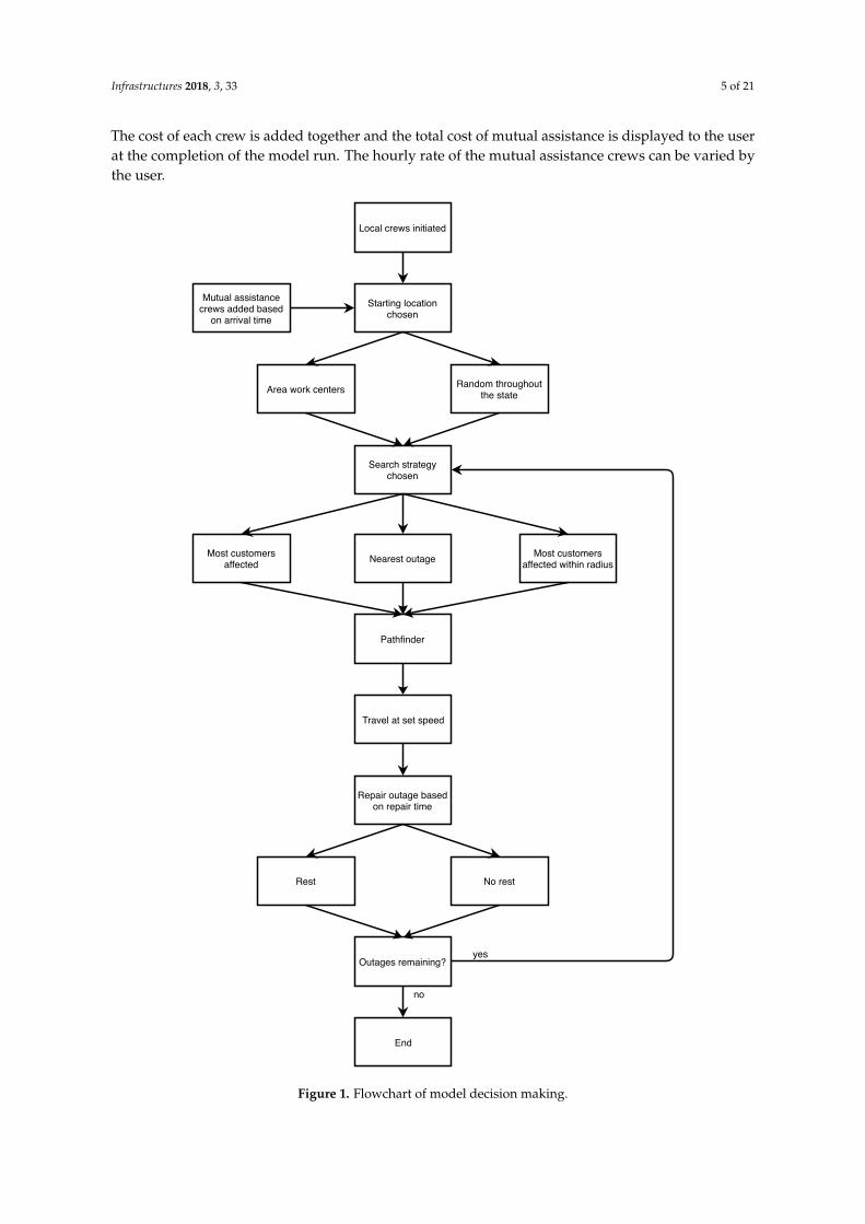
Once the ABM has gone through the setup process, the model follows an ordered procedurefor each tick. First, all of the crews determine the next outage they will go to if they do not alreadyhave an outage assigned to them. The options are either the (i) nearest outage, (ii) the outage with themost customers affected, (iii) finding the nearest outage then setting a radius around it and withinthat radius choosing the outage with the most customers affected, (iv) outage with the fastest repairtime, (v) finding the nearest outage then setting a radius around it and within that radius choosingthe outage with the fastest repair time, or (vi) outage with the fastest repair time and most customersaffected. The third option (which will be simplified as “nearest within radius”) simulates when crewscan travel a little further in order to have a greater impact on the number of customers still withoutpower. Once the crew determines its next outage, it changes the outage it found from “not taken” to“taken.” In the case where there are more crews than outages, crews may call off another crew if thecrew without an assigned outage is closer to the unrepaired outage. After a crew determines the outageit will travel to, Dijkstra’s routing algorithm is used to determine the shortest distance for the crew totravel along the road network to their assigned outage. The algorithm factors in the number and lengthof links to determine the optimal path. Dijkstra’s algorithm will determine the optimal path by findingthe combination of the least amount of links to travel and the overall shortest path [19]. Dijkstra’salgorithm has been used to model travelers taking public transportation and driving a vehicle [20].However, Dijkstra’s algorithm does not take power flow into consideration to prevent crews fromworking too close. Over a series of ticks, the crew will travel at a user defined speed until it reachesits outage. During the travel time, the outage will remain as “taken” and “unrepaired.” The crewwill stay at the outage and “work” for the user defined repair time assigned to the outage during thesetup. Once the crew finishes the repair, it will update the outage to “repaired” and check if the crewis next to take a break. If so, the crew’s break time will start and they will remain on break at theircurrent location for the next eight hours or the equivalent of one shift. Once the break is over, the crewwill select a new outage as long as there are still “unrepaired” outages. If all of the outages are set as“taken” but do not yet have a crew there working, a crew can call off another crew if they are closer.This simulates the end of a storm with utility companies trying to finish the remaining outages asquickly as possible. The model stops once no more crews are working and all of the outages have beenrepaired. Figure 1 illustrates the decisions made by the model.
As shown in Figure 1, mutual assistance crews may be arriving throughout the storm. At eachtick, the model does a check to see if any mutual assistance crews will be arriving. If so, the model willsprout new crews. Just like the initial crews, the mutual assistance crews will either start at AWCsor randomly across the state depending on the user chosen parameters. Once initiated, the mutualassistance crews operate identical to the original crews. Mutual assistance crews keep track of theirtravel time, their work time and their travel time back to where they started from. The model assumesmutual assistance crews begin traveling as the model starts running. Therefore, mutual assistancecrews can keep track of how long they traveled, the amount of time they worked and include theirtravel time back home. If the crew will be assisting a different utility after completing their work inConnecticut, the travel time back to their home state will not be included. The total time the mutualassistance crew was traveling and working for the utility is used to calculate the cost of their aid.
Infrastructures 2018, 3, 33 5 of 21
The cost of each crew is added together and the total cost of mutual assistance is displayed to the userat the completion of the model run. The hourly rate of the mutual assistance crews can be varied bythe user.
Local crews initiated
Starting locationchosen
Mutual assistancecrews added based
on arrival time
Area work centers Random throughoutthe state
Search strategychosen
Most customersaffected Nearest outage Most customers
affected within radius
Pathfinder
Travel at set speed
Repair outage basedon repair time
Rest No rest
Outages remaining?
End
yes
no
Figure 1. Flowchart of model decision making.
Infrastructures 2018, 3, 33 6 of 21
2.3. Model Validation
Model validation was completed utilizing past storm data and tested using different combinationsof parameters. These data included outage locations, number of customers affected and number ofcrews working. Since the nature of storm damage is different for each storm, outage repair times werevaried uniformly between lower and upper limits to optimize the fit compared to past storm restorationcurves. Moreover, the crew starting locations (area work center or random) and search strategy (nearest,most customers affected, most customers affected within a radius of the nearest outage, fastest repairtime, fastest repair time within a radius and fastest repair time with most customers affected) werealso varied to optimize the validation. Model fits were assessed using R2, mean absolute error (MAE)and standard deviation.
3. Results and Discussion
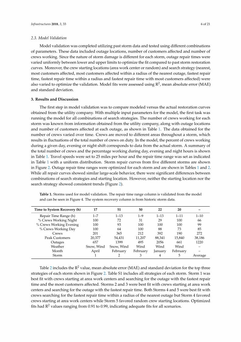
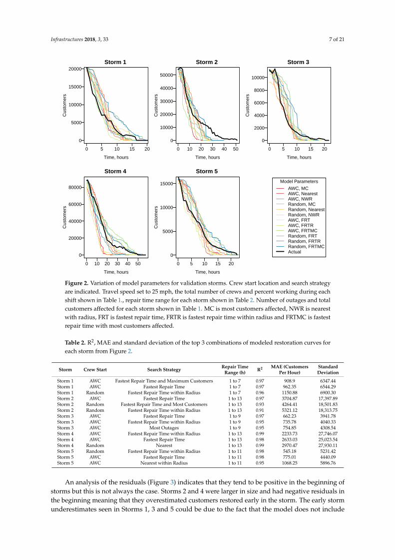
The first step in model validation was to compare modeled versus the actual restoration curvesobtained from the utility company. With multiple input parameters for the model, the first task wasrunning the model for all combinations of search strategies. The number of crews working for eachstorm was known from information obtained from the utility company, along with outage locationsand number of customers affected at each outage, as shown in Table 1. The data obtained for thenumber of crews varied over time. Crews are moved to different areas throughout a storm, whichresults in fluctuations of the total number of crews on duty. In the model, the percent of crews workingduring a given day, evening or night shift corresponds to data from the actual storm. A summary ofthe total number of crews and the percentage working during day, evening and night hours is shownin Table 1. Travel speeds were set to 25 miles per hour and the repair time range was set as indicatedin Table 1 with a uniform distribution. Storm repair curves from five different storms are shownin Figure 2. Outage repair time ranges were optimized for each storm and are shown in Tables 1 and 2.While all repair curves showed similar large-scale behavior, there were significant differences betweencombinations of search strategies and starting location. However, neither the starting location nor thesearch strategy showed consistent trends (Figure 2).
Table 1. Storms used for model validation. The repair time range column is validated from the modeland can be seen in Figure 4. The system recovery column is from historic storm data.
Time to System Recovery (h) 17 51 50 22 20 –
Repair Time Range (h) 1–7 1–13 1–9 1–13 1–11 1–10% Crews Working Night 100 72 31 29 100 66
% Crews Working Evening 100 93 100 100 100 99% Crews Working Day 100 64 100 88 73 85
Crews 201 365 212 392 190 272Peak Customers 20,377 54,431 11,207 88,341 15,840 38,186
Outages 657 1399 495 2056 661 1220Weather Snow, Wind Snow, Wind Wind Wind Wind –Month April February February January February –Storm 1 2 3 4 5 Average
Table 2 includes the R2 value, mean absolute error (MAE) and standard deviation for the top threestrategies of each storm shown in Figure 2. Table S1 includes all strategies of each storm. Storm 1 wasbest fit with crews starting at area work centers and searching for the outage with the fastest repairtime and the most customers affected. Storms 2 and 3 were best fit with crews starting at area workcenters and searching for the outage with the fastest repair time. Both Storms 4 and 5 were best fit withcrews searching for the fastest repair time within a radius of the nearest outage but Storm 4 favoredcrews starting at area work centers while Storm 5 favored random crew starting locations. Optimizedfits had R2 values ranging from 0.91 to 0.99, indicating adequate fits for all scenarios.
Infrastructures 2018, 3, 33 7 of 21
0 5 10 15 20
0
5000
10000
15000
20000Storm 1
Cus
tom
ers
Time, hours
0 10 20 30 40 50
0
10000
20000
30000
40000
50000
Storm 2
Cus
tom
ers
Time, hours
0 5 10 15 20
0
2000
4000
6000
8000
10000
Storm 3
Cus
tom
ers
Time, hours
0 10 20 30 40 50
0
20000
40000
60000
80000
Storm 4
Cus
tom
ers
Time, hours
0 5 10 15 20
0
5000
10000
15000
Storm 5
Cus
tom
ers
Time, hours
Model Parameters
AWC, MCAWC, NearestAWC, NWRRandom, MCRandom, NearestRandom, NWRAWC, FRTAWC, FRTRAWC, FRTMCRandom, FRTRandom, FRTRRandom, FRTMCActual
Figure 2. Variation of model parameters for validation storms. Crew start location and search strategyare indicated. Travel speed set to 25 mph, the total number of crews and percent working during eachshift shown in Table 1., repair time range for each storm shown in Table 2. Number of outages and totalcustomers affected for each storm shown in Table 1. MC is most customers affected, NWR is nearestwith radius, FRT is fastest repair time, FRTR is fastest repair time within radius and FRTMC is fastestrepair time with most customers affected.
Table 2. R2, MAE and standard deviation of the top 3 combinations of modeled restoration curves foreach storm from Figure 2.
Storm Crew Start Search Strategy Repair TimeRange (h) R2 MAE (Customers
Per Hour)StandardDeviation
Storm 1 AWC Fastest Repair Time and Maximum Customers 1 to 7 0.97 908.9 6347.44Storm 1 AWC Fastest Repair Time 1 to 7 0.97 962.35 6544.29Storm 1 Random Fastest Repair Time within Radius 1 to 7 0.96 1150.88 6900.30Storm 2 AWC Fastest Repair Time 1 to 13 0.97 3704.87 17,397.89Storm 2 Random Fastest Repair Time and Most Customers 1 to 13 0.93 4264.41 18,501.83Storm 2 Random Fastest Repair Time within Radius 1 to 13 0.91 5321.12 18,313.75Storm 3 AWC Fastest Repair Time 1 to 9 0.97 662.23 3941.78Storm 3 AWC Fastest Repair Time within Radius 1 to 9 0.95 735.78 4040.33Storm 3 AWC Most Outages 1 to 9 0.95 754.85 4308.54Storm 4 AWC Fastest Repair Time within Radius 1 to 13 0.99 2233.73 27,746.07Storm 4 AWC Fastest Repair Time 1 to 13 0.98 2633.03 25,023.54Storm 4 Random Nearest 1 to 13 0.99 2970.47 27,930.11Storm 5 Random Fastest Repair Time within Radius 1 to 11 0.98 545.18 5231.42Storm 5 AWC Fastest Repair Time 1 to 11 0.98 775.01 4440.09Storm 5 AWC Nearest within Radius 1 to 11 0.95 1068.25 5896.76
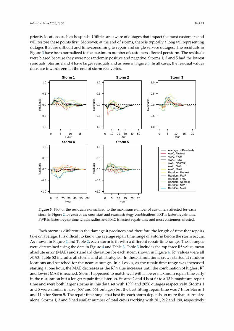
An analysis of the residuals (Figure 3) indicates that they tend to be positive in the beginning ofstorms but this is not always the case. Storms 2 and 4 were larger in size and had negative residuals inthe beginning meaning that they overestimated customers restored early in the storm. The early stormunderestimates seen in Storms 1, 3 and 5 could be due to the fact that the model does not include
Infrastructures 2018, 3, 33 8 of 21
priority locations such as hospitals. Utilities are aware of outages that impact the most customers andwill restore these points first. Moreover, at the end of storms, there is typically a long tail representingoutages that are difficult and time-consuming to repair and single service outages. The residuals inFigure 3 have been normalized to the maximum number of customers affected per storm. The residualswere biased because they were not randomly positive and negative. Storms 1, 3 and 5 had the lowestresiduals. Storms 2 and 4 have larger residuals and as seen in Figure 3. In all cases, the residual valuesdecrease towards zero at the end of storm recoveries.
0 5 10 15
−1.0
−0.5
0.0
0.5
1.0
Storm 1
Res
idua
ls
Hour0 10 20 30 40 50
−1.0
−0.5
0.0
0.5
1.0
Storm 2
Res
idua
ls
Hour0 5 10 15 20
−1.0
−0.5
0.0
0.5
1.0
Storm 3
Res
idua
ls
Hour
0 10 20 30 40 50 60
−1.0
−0.5
0.0
0.5
1.0
Storm 4
Res
idua
ls
Hour0 5 10 15 20 25
−1.0
−0.5
0.0
0.5
1.0
Storm 5
Res
idua
ls
Hour
Average of ResidualsAWC, FastestAWC, FWRAWC, FMCAWC, NearestAWC, NWRAWC, MostRandom, FastestRandom, FWRRandom, FMCRandom, NearestRandom, NWRRandom, Most
Figure 3. Plot of the residuals normalized to the maximum number of customers affected for eachstorm in Figure 2 for each of the crew start and search strategy combinations. FRT is fastest repair time,FWR is fastest repair time within radius and FMC is fastest repair time and most customers affected.
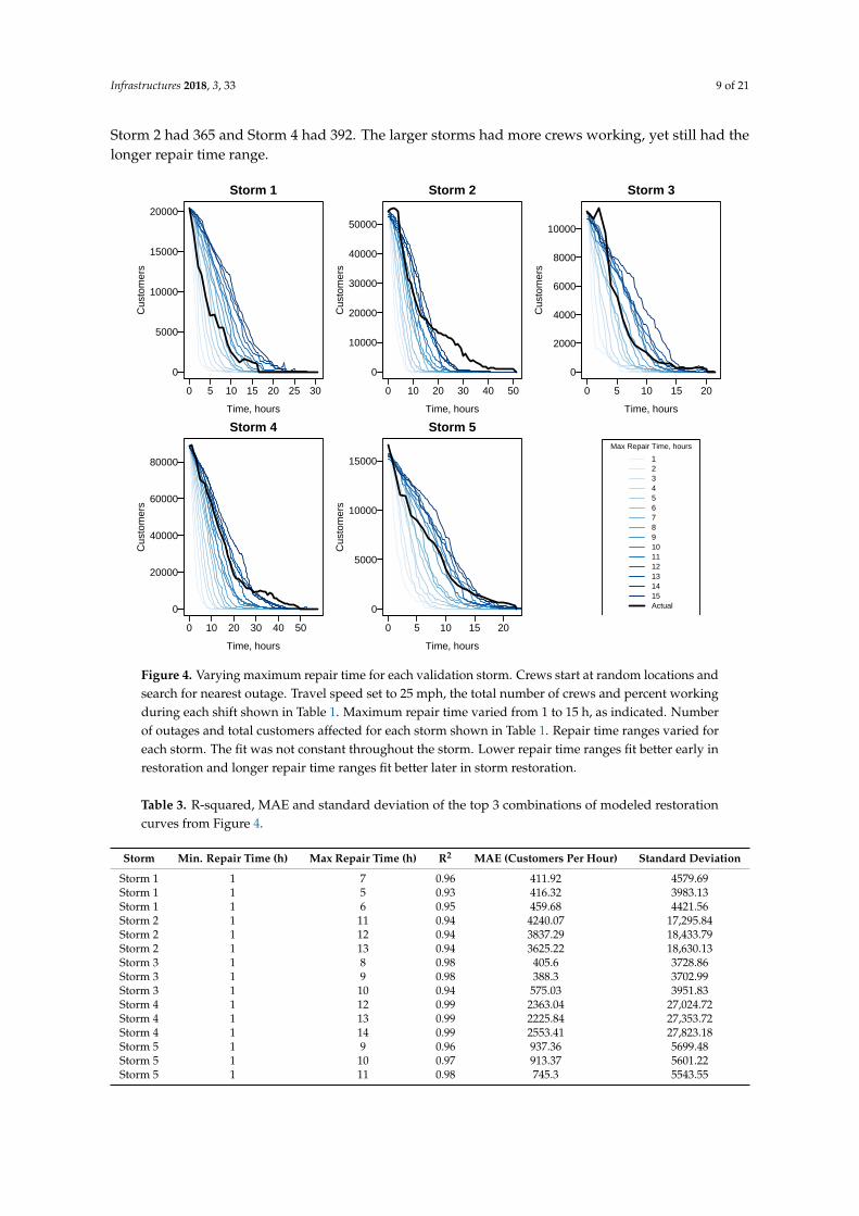
Each storm is different in the damage it produces and therefore the length of time that repairstake on average. It is difficult to know the average repair time range of a storm before the storm occurs.As shown in Figure 2 and Table 2, each storm is fit with a different repair time range. These rangeswere determined using the data in Figure 4 and Table 3. Table 3 includes the top three R2 value, meanabsolute error (MAE) and standard deviation for each storm shown in Figure 4. R2 values were all>0.93. Table S2 includes all storms and all strategies. In these simulations, crews started at randomlocations and searched for the nearest outage. In all cases, as the repair time range was increasedstarting at one hour, the MAE decreases as the R2 value increases until the combination of highest R2
and lowest MAE is reached. Storm 1 appeared to match well with a lower maximum repair time earlyin the restoration but a longer repair time later on. Storms 2 and 4 best fit to a 13 h maximum repairtime and were both larger storms in this data set with 1399 and 2056 outages respectively. Storms 1and 5 were similar in size (657 and 661 outages) but the best fitting repair time was 7 h for Storm 1and 11 h for Storm 5. The repair time range that best fits each storm depends on more than storm sizealone. Storms 1, 3 and 5 had similar number of total crews working with 201, 212 and 190, respectively.
Infrastructures 2018, 3, 33 9 of 21
Storm 2 had 365 and Storm 4 had 392. The larger storms had more crews working, yet still had thelonger repair time range.
0 5 10 15 20 25 30
0
5000
10000
15000
20000
Storm 1
Cus
tom
ers
Time, hours
0 10 20 30 40 50
0
10000
20000
30000
40000
50000
Storm 2
Cus
tom
ers
Time, hours
0 5 10 15 20
0
2000
4000
6000
8000
10000
Storm 3
Cus
tom
ers
Time, hours
0 10 20 30 40 50
0
20000
40000
60000
80000
Storm 4
Cus
tom
ers
Time, hours
0 5 10 15 20
0
5000
10000
15000
Storm 5
Cus
tom
ers
Time, hours
Max Repair Time, hours
123456789101112131415Actual
Figure 4. Varying maximum repair time for each validation storm. Crews start at random locations andsearch for nearest outage. Travel speed set to 25 mph, the total number of crews and percent workingduring each shift shown in Table 1. Maximum repair time varied from 1 to 15 h, as indicated. Numberof outages and total customers affected for each storm shown in Table 1. Repair time ranges varied foreach storm. The fit was not constant throughout the storm. Lower repair time ranges fit better early inrestoration and longer repair time ranges fit better later in storm restoration.
Table 3. R-squared, MAE and standard deviation of the top 3 combinations of modeled restorationcurves from Figure 4.
Storm Min. Repair Time (h) Max Repair Time (h) R2 MAE (Customers Per Hour) Standard Deviation
Storm 1 1 7 0.96 411.92 4579.69Storm 1 1 5 0.93 416.32 3983.13Storm 1 1 6 0.95 459.68 4421.56Storm 2 1 11 0.94 4240.07 17,295.84Storm 2 1 12 0.94 3837.29 18,433.79Storm 2 1 13 0.94 3625.22 18,630.13Storm 3 1 8 0.98 405.6 3728.86Storm 3 1 9 0.98 388.3 3702.99Storm 3 1 10 0.94 575.03 3951.83Storm 4 1 12 0.99 2363.04 27,024.72Storm 4 1 13 0.99 2225.84 27,353.72Storm 4 1 14 0.99 2553.41 27,823.18Storm 5 1 9 0.96 937.36 5699.48Storm 5 1 10 0.97 913.37 5601.22Storm 5 1 11 0.98 745.3 5543.55
Infrastructures 2018, 3, 33 10 of 21
3.1. Model Sensitivity
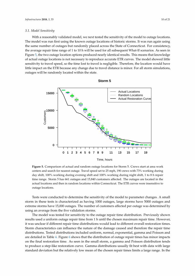
With a reasonably validated model, we next tested the sensitivity of the model to outage locations.The model was run first using the known outage locations of historic storms. It was run again usingthe same number of outages but randomly placed across the State of Connecticut. For consistency,the average repair time range of 1 to 10 h will be used for all subsequent What-If scenarios. As seen inFigure 5, the two outage location options produced nearly identical results. This means that knowledgeof actual outage locations is not necessary to reproduce accurate ETR curves. The model showed littlesensitivity to travel speed, so the time lost to travel is negligible. Therefore, the location would havelittle impact on the ETR because any change due to travel distance is minor. For all storm simulations,outages will be randomly located within the state.
0 1 2 3 4 5 6 7 8 9 11 13 15 17 19
0
5000
10000
15000
Storm 5
Time, hours
0 1 2 3 4 5 6 7 8 9 11 13 15 17 19
0
5000
10000
15000
Cus
tom
ers
Actual LocationsRandom LocationsActual Restoration Curve
Figure 5. Comparison of actual and random outage locations for Storm 5. Crews start at area workcenters and search for nearest outage. Travel speed set to 25 mph, 190 crews with 73% working duringday shift, 100% working during evening shift and 100% working during night shift, 1 to 8 h repairtime range. Storm 5 has 661 outages and 15,840 customers affected. The outages are located in theactual locations and then in random locations within Connecticut. The ETR curves were insensitive tooutage locations.
Tests were conducted to determine the sensitivity of the model to parameter changes. A smallstorm in these tests is characterized as having 1000 outages, large storms have 5000 outages andextreme storms have 15,000 outages. The number of customers affected per outage was determined byusing an average from the five validation storms.
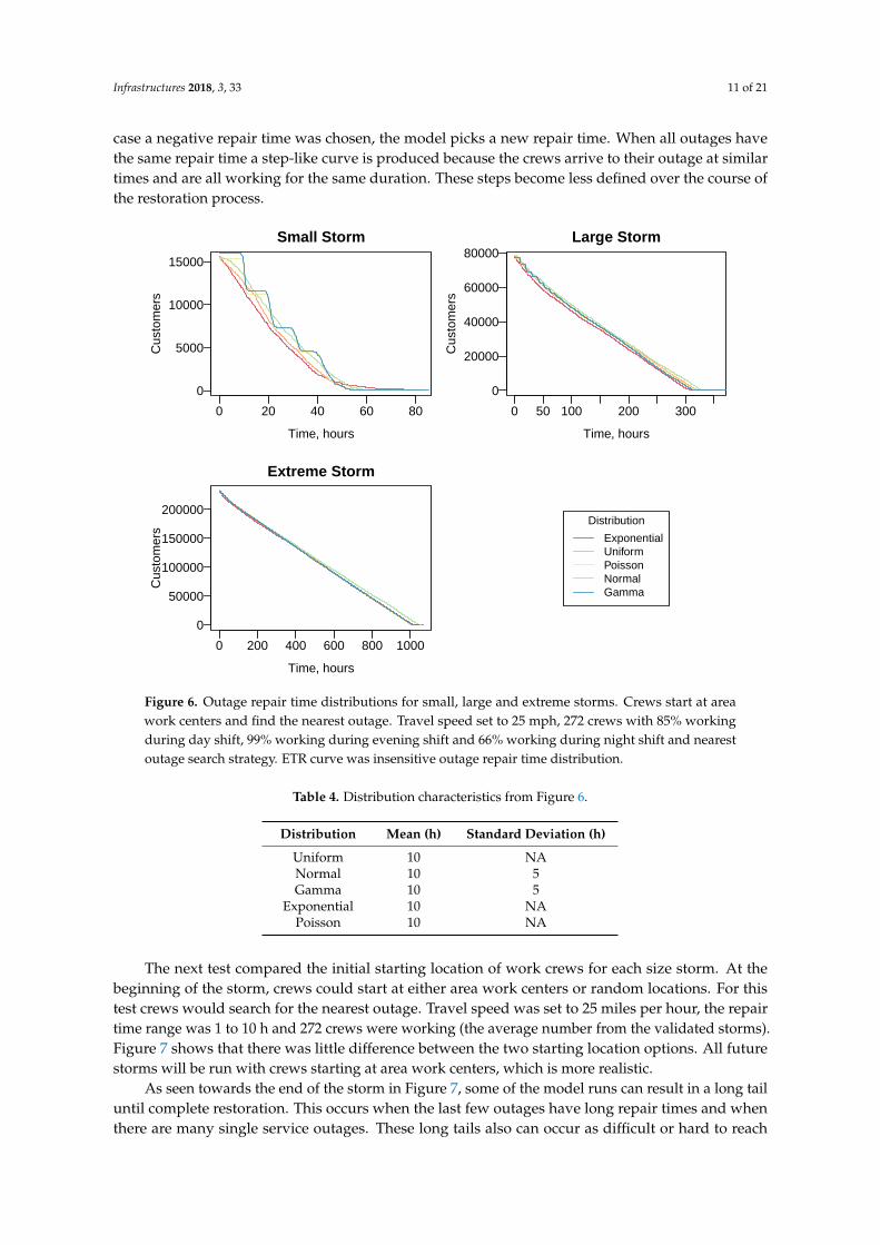
The model was tested for sensitivity to the outage repair time distribution. Previously shownresults used a uniform outage repair time from 1 h until the chosen maximum repair time. However,it was unclear if different repair time distributions would lead to different overall restoration times.Storm characteristics can influence the nature of the damage caused and therefore the repair timedistributions. Tested distributions included uniform, normal, exponential, gamma and Poisson andare detailed in Table 4. Figure 6 shows that the distribution of outage repair times has minor impactson the final restoration time. As seen in the small storm, a gamma and Poisson distribution tendsto produce a step-like restoration curve. Gamma distributions usually fit best with data with largestandard deviation but the relatively low mean of the chosen repair times limits a large range. In the
Infrastructures 2018, 3, 33 11 of 21
case a negative repair time was chosen, the model picks a new repair time. When all outages havethe same repair time a step-like curve is produced because the crews arrive to their outage at similartimes and are all working for the same duration. These steps become less defined over the course ofthe restoration process.
0 20 40 60 80
0
5000
10000
15000
Small Storm
Cus
tom
ers
Time, hours
0 50 100 200 300
0
20000
40000
60000
80000Large Storm
Cus
tom
ers
Time, hours
0 200 400 600 800 1000
0
50000
100000
150000
200000
Extreme Storm
Cus
tom
ers
Time, hours
Distribution
ExponentialUniformPoissonNormalGamma
Figure 6. Outage repair time distributions for small, large and extreme storms. Crews start at areawork centers and find the nearest outage. Travel speed set to 25 mph, 272 crews with 85% workingduring day shift, 99% working during evening shift and 66% working during night shift and nearestoutage search strategy. ETR curve was insensitive outage repair time distribution.
Table 4. Distribution characteristics from Figure 6.
Distribution Mean (h) Standard Deviation (h)
Uniform 10 NANormal 10 5Gamma 10 5
Exponential 10 NAPoisson 10 NA
The next test compared the initial starting location of work crews for each size storm. At thebeginning of the storm, crews could start at either area work centers or random locations. For thistest crews would search for the nearest outage. Travel speed was set to 25 miles per hour, the repairtime range was 1 to 10 h and 272 crews were working (the average number from the validated storms).Figure 7 shows that there was little difference between the two starting location options. All futurestorms will be run with crews starting at area work centers, which is more realistic.
As seen towards the end of the storm in Figure 7, some of the model runs can result in a long tailuntil complete restoration. This occurs when the last few outages have long repair times and whenthere are many single service outages. These long tails also can occur as difficult or hard to reach

Infrastructures 2018, 3, 33 12 of 21
repairs are often left until the end. To highlight the major scenario differences, all ETR curves will becropped when the number of customers remaining without power was no more than 20 for the smallstorm and 100 for the large and extreme storms. Figures S1–S3 for small and extreme storms can befound in the Supplementary Materials.
0 50 100 150
0
20000
40000
60000
80000
Large Storm
Time, hours
Cus
tom
ers
Start Location
Area Work CenterRandom
Figure 7. Start location for simulated large storms with 5000 outages. Crew start location varied asindicated. Travel speed set to 25 mph, 272 crews with 85% working during day shift, 99% workingduring evening shift and 66% working during night shift, 1 to 10 h repair time range and nearest outagesearch strategy. ETR curve was insensitive to crew start location.
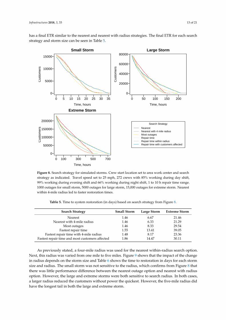
Next, the crew search strategy was varied between nearest outage, the outage with the mostcustomers affected within a radius of the nearest outage (nearest within radius), the outage with themost customers affected, the outage with the fastest repair time, the outage with the fastest repair timewithin a radius of the nearest outage and the outage with the fastest repair time and most customersaffected. All of the parameters were kept the same as previously described and crews started at areawork centers. The radius was set to four miles for the nearest within radius and fastest within radiussearch options. Figure 8 shows some sensitivity to search strategy, especially in the large and extremestorms. For the small storm, there was little difference between the nearest outage, nearest with radiusand fastest repair time. The most customers affected option performed better in the beginning buta longer tail at the end lengthened the final ETR. The large storm shows a bigger difference betweenthe nearest outage and nearest with radius options. However, the nearest within radius performedsimilar to the most outages option in the beginning but ended faster than most outages. The nearestand nearest within radius search strategies had similar ETRs for the large storm but nearest withinradius always had less customers still without power than nearest. The biggest differences betweensearch options came in the extreme storm situation. The nearest within radius option performed bestthroughout the run. In the beginning of the simulation most outages performed between nearestwithin radius option and nearest outage, until about the 400-h point. After the 400-h mark, the mostoutages option reduced the number of customers affected most slowly. The nearest within radiusoption reduced the number of customers affected the fastest and had an ETR closest to the nearestsearch strategy. In both the large and extreme storms, the search strategies using repair times havesimilar impacts on the ETR curves. Both fastest repair time and fastest with most customers have thelongest final ETR. The fastest within radius performs the best in the beginning of the storm but then
Infrastructures 2018, 3, 33 13 of 21
has a final ETR similar to the nearest and nearest with radius strategies. The final ETR for each searchstrategy and storm size can be seen in Table 5.
0 5 10 15 20 25 30 35
0
5000
10000
15000
Small Storm
Cus
tom
ers
Time, hours
0 50 100 150 200
0
20000
40000
60000
80000Large Storm
Cus
tom
ers
Time, hours
0 100 300 500 700
0
50000
100000
150000
200000
Extreme Storm
Cus
tom
ers
Time, hours
Search Strategy
NearestNearest with 4 mile radiusMost outagesRepair timeRepair time within radiusRepair time with customers affected
Figure 8. Search strategy for simulated storms. Crew start location set to area work center and searchstrategy as indicated. Travel speed set to 25 mph, 272 crews with 85% working during day shift,99% working during evening shift and 66% working during night shift, 1 to 10 h repair time range.1000 outages for small storm, 5000 outages for large storm, 15,000 outages for extreme storm. Nearestwithin 4-mile radius led to faster restoration times.
Table 5. Time to system restoration (in days) based on search strategy from Figure 8.
Search Strategy Small Storm Large Storm Extreme Storm
Nearest 1.46 6.67 21.46Nearest with 4-mile radius 1.46 6.33 21.29
Most outages 1.46 8.33 29.54Fastest repair time 1.55 13.41 39.05
Fastest repair time with 4-mile radius 1.48 8.17 23.36Fastest repair time and most customers affected 1.86 14.47 30.11
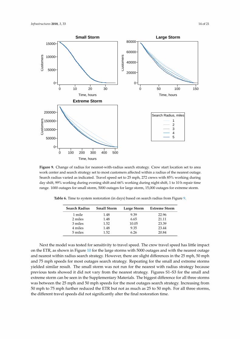
As previously stated, a four-mile radius was used for the nearest within-radius search option.Next, this radius was varied from one mile to five miles. Figure 9 shows that the impact of the changein radius depends on the storm size and Table 6 shows the time to restoration in days for each stormsize and radius. The small storm was not sensitive to the radius, which confirms from Figure 8 thatthere was little performance difference between the nearest outage option and nearest with radiusoption. However, the large and extreme storms were both sensitive to search radius. In both cases,a larger radius reduced the customers without power the quickest. However, the five-mile radius didhave the longest tail in both the large and extreme storm.
Infrastructures 2018, 3, 33 14 of 21
0 10 20 30
0
5000
10000
15000
Small StormC
usto
mer
s
Time, hours
0 50 100 150
0
20000
40000
60000
80000Large Storm
Cus
tom
ers
Time, hours
0 100 200 300 400 500
0
50000
100000
150000
200000
Extreme Storm
Cus
tom
ers
Time, hours
Search Radius, miles
12345
Figure 9. Change of radius for nearest-with-radius search strategy. Crew start location set to areawork center and search strategy set to most customers affected within a radius of the nearest outage.Search radius varied as indicated. Travel speed set to 25 mph, 272 crews with 85% working duringday shift, 99% working during evening shift and 66% working during night shift, 1 to 10 h repair timerange. 1000 outages for small storm, 5000 outages for large storm, 15,000 outages for extreme storm.
Table 6. Time to system restoration (in days) based on search radius from Figure 9.
Search Radius Small Storm Large Storm Extreme Storm
1 mile 1.48 9.39 22.962 miles 1.48 6.65 21.113 miles 1.52 10.05 23.394 miles 1.48 9.35 23.445 miles 1.52 6.26 20.84
Next the model was tested for sensitivity to travel speed. The crew travel speed has little impacton the ETR, as shown in Figure 10 for the large storms with 5000 outages and with the nearest outageand nearest within radius search strategy. However, there are slight differences in the 25 mph, 50 mphand 75 mph speeds for most outages search strategy. Repeating for the small and extreme stormsyielded similar result. The small storm was not run for the nearest with radius strategy becauseprevious tests showed it did not vary from the nearest strategy. Figures S1–S3 for the small andextreme storm can be seen in the Supplementary Materials. The biggest difference for all three stormswas between the 25 mph and 50 mph speeds for the most outages search strategy. Increasing from50 mph to 75 mph further reduced the ETR but not as much as 25 to 50 mph. For all three storms,the different travel speeds did not significantly alter the final restoration time.
Infrastructures 2018, 3, 33 15 of 21
0 100 200 300 400 500
0
50000
100000
150000
200000
Nearest OutageC
usto
mer
s
Time, hours
0 100 200 300 400 500
0
50000
100000
150000
200000
Nearest within Radius
Cus
tom
ers
Time, hours
0 100 300 500 700
0
50000
100000
150000
200000
Most Customers Affected
Cus
tom
ers
Time, hours
Travel Speed, miles per hour
255075
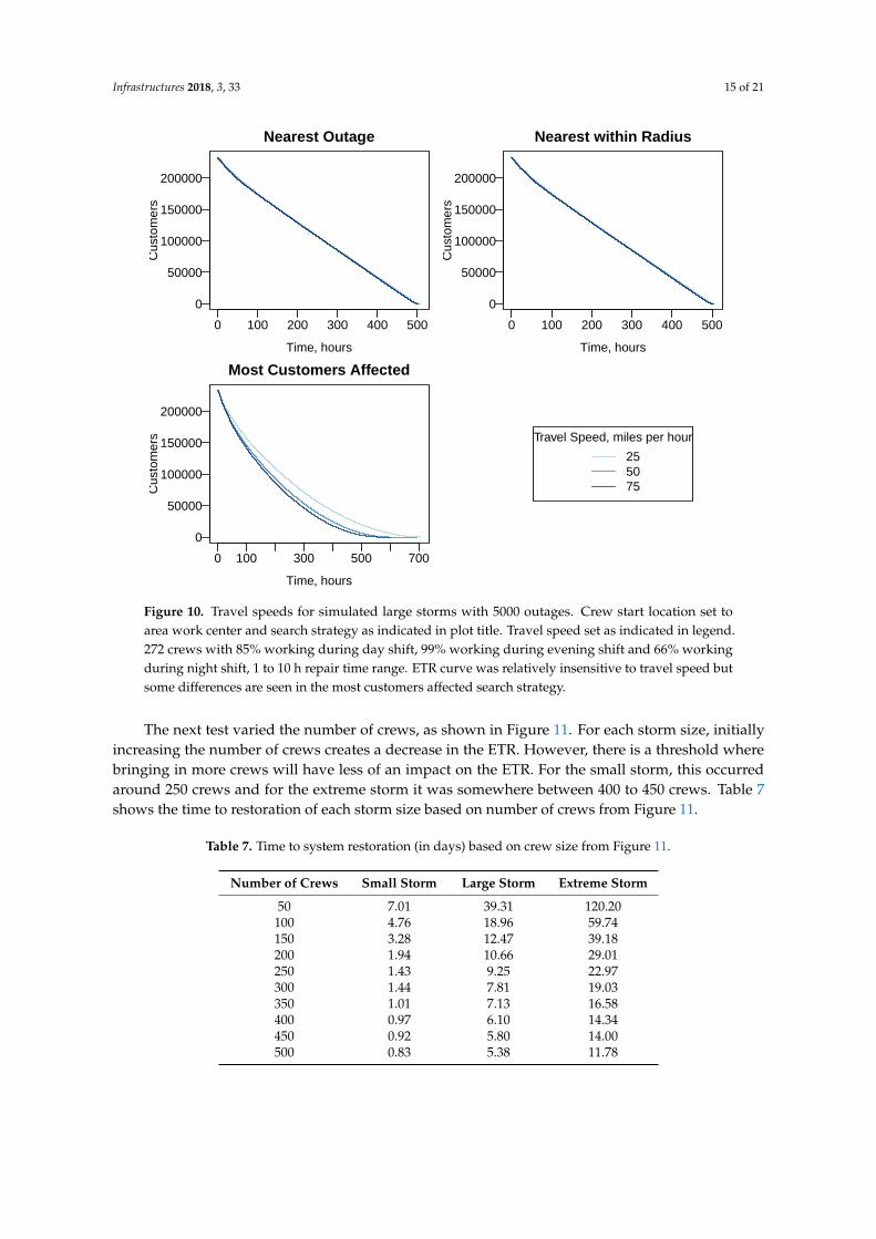
Figure 10. Travel speeds for simulated large storms with 5000 outages. Crew start location set toarea work center and search strategy as indicated in plot title. Travel speed set as indicated in legend.272 crews with 85% working during day shift, 99% working during evening shift and 66% workingduring night shift, 1 to 10 h repair time range. ETR curve was relatively insensitive to travel speed butsome differences are seen in the most customers affected search strategy.
The next test varied the number of crews, as shown in Figure 11. For each storm size, initiallyincreasing the number of crews creates a decrease in the ETR. However, there is a threshold wherebringing in more crews will have less of an impact on the ETR. For the small storm, this occurredaround 250 crews and for the extreme storm it was somewhere between 400 to 450 crews. Table 7shows the time to restoration of each storm size based on number of crews from Figure 11.
Table 7. Time to system restoration (in days) based on crew size from Figure 11.
Number of Crews Small Storm Large Storm Extreme Storm
50 7.01 39.31 120.20100 4.76 18.96 59.74150 3.28 12.47 39.18200 1.94 10.66 29.01250 1.43 9.25 22.97300 1.44 7.81 19.03350 1.01 7.13 16.58400 0.97 6.10 14.34450 0.92 5.80 14.00500 0.83 5.38 11.78
Infrastructures 2018, 3, 33 16 of 21
50 150 250 350 450
2
4
6
8
10
Small Storm
ET
R, d
ays
Crews50 150 250 350 450
10
20
30
40
Large Storm
ET
R, d
ays
Crews
50 150 250 350 450
20
40
60
80
100
120
Extreme Storm
ET
R, d
ays
Crews
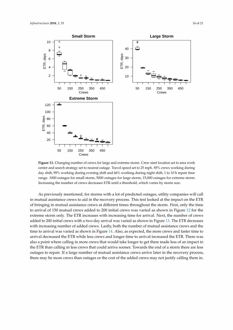
Figure 11. Changing number of crews for large and extreme storm. Crew start location set to area workcenter and search strategy set to nearest outage. Travel speed set to 25 mph. 85% crews working duringday shift, 99% working during evening shift and 66% working during night shift, 1 to 10 h repair timerange. 1000 outages for small storm, 5000 outages for large storm, 15,000 outages for extreme storm.Increasing the number of crews decreases ETR until a threshold, which varies by storm size.
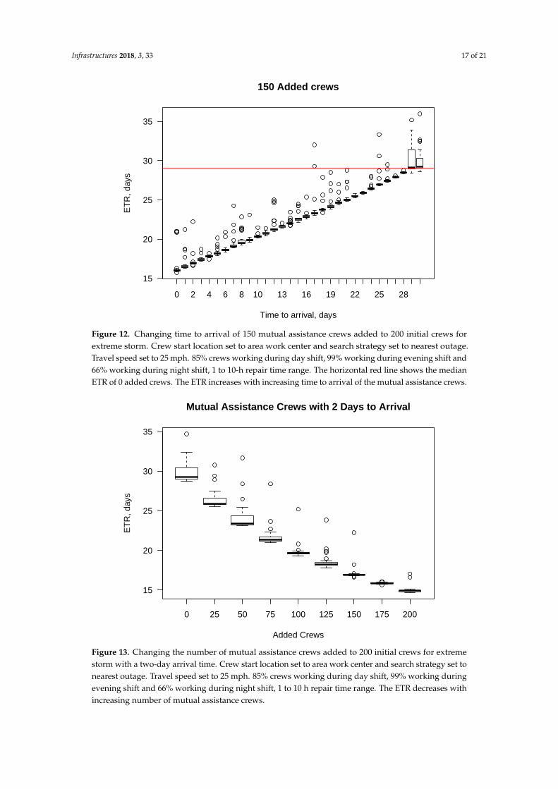
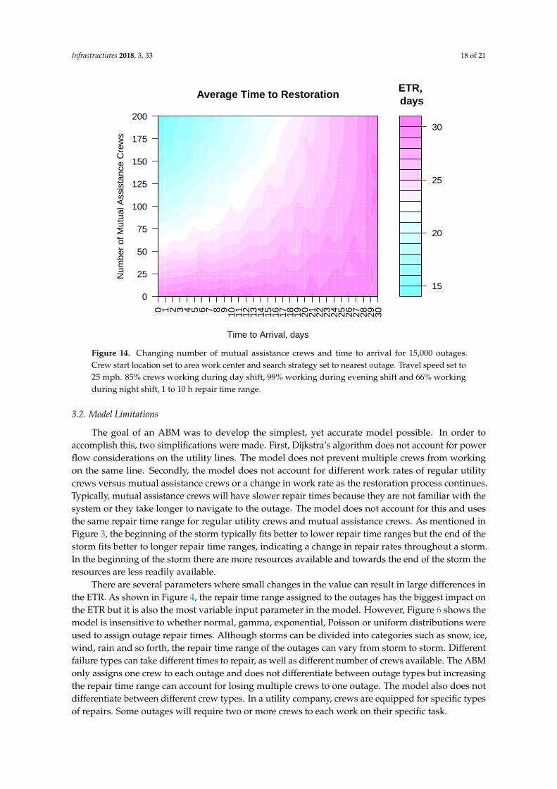
As previously mentioned, for storms with a lot of predicted outages, utility companies will callin mutual assistance crews to aid in the recovery process. This test looked at the impact on the ETRof bringing in mutual assistance crews at different times throughout the storm. First, only the timeto arrival of 150 mutual crews added to 200 initial crews was varied as shown in Figure 12 for theextreme storm only. The ETR increases with increasing time for arrival. Next, the number of crewsadded to 200 initial crews with a two-day arrival was varied as shown in Figure 13. The ETR decreaseswith increasing number of added crews. Lastly, both the number of mutual assistance crews and thetime to arrival was varied as shown in Figure 14. Also, as expected, the more crews and faster time toarrival decreased the ETR while less crews and longer time to arrival increased the ETR. There wasalso a point where calling in more crews that would take longer to get there made less of an impact inthe ETR than calling in less crews that could arrive sooner. Towards the end of a storm there are lessoutages to repair. If a large number of mutual assistance crews arrive later in the recovery process,there may be more crews than outages or the cost of the added crews may not justify calling them in.
Infrastructures 2018, 3, 33 17 of 21
0 2 4 6 8 10 13 16 19 22 25 28
15
20
25
30
35
150 Added crews
Time to arrival, days
ET
R, d
ays
Figure 12. Changing time to arrival of 150 mutual assistance crews added to 200 initial crews forextreme storm. Crew start location set to area work center and search strategy set to nearest outage.Travel speed set to 25 mph. 85% crews working during day shift, 99% working during evening shift and66% working during night shift, 1 to 10-h repair time range. The horizontal red line shows the medianETR of 0 added crews. The ETR increases with increasing time to arrival of the mutual assistance crews.
0 25 50 75 100 125 150 175 200
15
20
25
30
35
Mutual Assistance Crews with 2 Days to Arrival
Added Crews
ET
R, d
ays
Figure 13. Changing the number of mutual assistance crews added to 200 initial crews for extremestorm with a two-day arrival time. Crew start location set to area work center and search strategy set tonearest outage. Travel speed set to 25 mph. 85% crews working during day shift, 99% working duringevening shift and 66% working during night shift, 1 to 10 h repair time range. The ETR decreases withincreasing number of mutual assistance crews.
Infrastructures 2018, 3, 33 18 of 21
15
20
25
30
ETR, days
0 1 2 3 4 5 6 7 8 9 10 11 12 13 14 15 16 17 18 19 20 21 22 23 24 25 26 27 28 29 30
0
25
50
75
100
125
150
175
200
Average Time to Restoration
Time to Arrival, days
Num
ber
of M
utua
l Ass
ista
nce
Cre
ws
Figure 14. Changing number of mutual assistance crews and time to arrival for 15,000 outages.Crew start location set to area work center and search strategy set to nearest outage. Travel speed set to25 mph. 85% crews working during day shift, 99% working during evening shift and 66% workingduring night shift, 1 to 10 h repair time range.
3.2. Model Limitations
The goal of an ABM was to develop the simplest, yet accurate model possible. In order toaccomplish this, two simplifications were made. First, Dijkstra’s algorithm does not account for powerflow considerations on the utility lines. The model does not prevent multiple crews from workingon the same line. Secondly, the model does not account for different work rates of regular utilitycrews versus mutual assistance crews or a change in work rate as the restoration process continues.Typically, mutual assistance crews will have slower repair times because they are not familiar with thesystem or they take longer to navigate to the outage. The model does not account for this and usesthe same repair time range for regular utility crews and mutual assistance crews. As mentioned inFigure 3, the beginning of the storm typically fits better to lower repair time ranges but the end of thestorm fits better to longer repair time ranges, indicating a change in repair rates throughout a storm.In the beginning of the storm there are more resources available and towards the end of the storm theresources are less readily available.
There are several parameters where small changes in the value can result in large differences inthe ETR. As shown in Figure 4, the repair time range assigned to the outages has the biggest impact onthe ETR but it is also the most variable input parameter in the model. However, Figure 6 shows themodel is insensitive to whether normal, gamma, exponential, Poisson or uniform distributions wereused to assign outage repair times. Although storms can be divided into categories such as snow, ice,wind, rain and so forth, the repair time range of the outages can vary from storm to storm. Differentfailure types can take different times to repair, as well as different number of crews available. The ABMonly assigns one crew to each outage and does not differentiate between outage types but increasingthe repair time range can account for losing multiple crews to one outage. The model also does notdifferentiate between different crew types. In a utility company, crews are equipped for specific typesof repairs. Some outages will require two or more crews to each work on their specific task.
Infrastructures 2018, 3, 33 19 of 21
The number of crews working and both the number and arrival time of mutual assistance crewscan vary throughout a storm. The model simplified these changes for the number of crews by havinga percentage of the total crews “resting.” The crews did not leave the model but did not contribute tothe restoration process during that time. During storm recovery, mutual assistance crews can arriveat different times and in different groups. To allow the user to easily input any mutual aid crews,all crews enter the model at the same time.
4. Conclusions
We developed an ABM using the NetLogo platform [19] to demonstrate that ABMs can bean important approach to power outage restoration after storms and can be beneficial to utilitycompanies. The ABM shows that different outage search strategies result in different ETR curves;the travel speed of crews has a minor impact on the ETR; increasing the number of crews will decreasethe ETR but only to a threshold; and the impact of mutual assistance crews depends on both thenumber of crews and their time to arrival.
This decision support tool has the following advantages compared to current methods:
• It is a quantitative tool based on empirical data that can be used by emergency managers to testa variety of restoration strategies.
• The model could be utilized prior to a storm based on outage predictions [21–26] or in real-timeas outages are discovered.
• It is a socio-technical model that integrates human decisions constrained by the physical infrastructure.• This is a decision support tool for utility managers to supplement current restoration time
estimates. Utility managers can test decisions prior to or during a storm to make necessaryadjustments to the restoration process including the decision to hire foreign crews.
• Providing a range of values for input variables can give a probabilistic range of outcomes for finalETRs. These probabilistic forecasts can be useful for utility companies to provide customers witha range of estimated restoration times.
• The model is easily transferable to other states or regions and would only require the roadnetwork dataset.
The developed ABM incorporates parameters not previously included in regression models, suchas the number of crews working and user defined rules to simulate crew behavior. The crews in themodel respond to the decisions made by the user, instead of using a statistical approach based on pastdata. The model can be used to determine the appropriate number of crews in order to reach a desiredETR and where and when foreign crews may be needed to achieve those goals. The model could beused to help estimate restoration times for policymakers and customers.
An important disadvantage of the ABM as it is currently structured is that it is computationallyintensive. There are many input variables and running the model over a range of all of these variablescan take a long time, especially for larger storms. The current ABM does not incorporate power flowconsiderations, like the expert systems approach developed by Liu et al. [8] does. The expert systemsapproach determined the optimal repair order based on minimizing losses and does not incorporatethe social interactions of crews.
In the future, this novel technique could be incorporated with outage predictions before stormshit [23–26] to give emergency managers a powerful tool to decrease restoration times in Connecticutand elsewhere. Cost of restoration and mutual assistance crews can be easily added to the model.This added feature would allow utility managers to see the impact their decision would have onthe cost to the utility company. The ABM could be used to explore the economic and restorationtime benefits of resilience measures, such as tree trimming. Lastly, the ABM could be developed asa training tool for new emergency managers.
Overall, this model is an important first step in a new approach to power restoration that couldbenefit both utility companies and utility customers.
Infrastructures 2018, 3, 33 20 of 21
Supplementary Materials: The following are available online at http://www.mdpi.com/2412-3811/3/3/33/s1,Table S1: R2, MAE and standard deviation of modeled restoration curves from Figure 2, Table S2. R2, MAE andstandard deviation of modeled restoration curves from Figure 4. Figure S1: Start location of crews for small andextreme storms, Figure S2: Crew travel speeds for small storms, Figure S3: Crew travel speeds for extreme storms,Agent Based Model for Storm Recovery Code.
Author Contributions: D.W. and J.M. developed the research idea; T.W. and J.M. were the primary programdevelopers; T.W. and J.M. conducted the data analysis; T.L. and D.W. provided data and industry expertise.
Funding: This research was funded by Department of Education grant number P200A150311 and EversourceEnergy Center.
Acknowledgments: The authors gratefully acknowledge the support provided by Emmanouil Anagnostou andthe UConn Eversource Energy Center.
Conflicts of Interest: The authors declare no conflict of interest.
References
1. Campbell, R.J. Weather-Related Power Outages and Electric System Resiliency. In Congressional ResearchService Report, (R42696); Congressional Research Service, Library of Congress: Washington, DC, USA, 2012;pp. 1–15.
2. Carolina, N.; Eastern, N.N.; Carolina, N. OE-417 Electric Emergency and Disturbance Report; Office ofCybersecurity, Energy Security, & Emergency Response: Washington, DC, USA, 2015; pp. 1–7.
3. Pachauri, R.K.; Allen, M.R.; Barros, V.R.; Broome, J.; Cramer, W.; Christ, R.; Church, J.A.; Clarke, L.; Dahe, Q.;Dasgupta, P.; et al. Summary for Policymakers. Climate Change 2014: Synthesis Report. Contribution of WorkingGroups I, II and III to the Fifth Assessment Report of the Intergovernmental Panel on Climate Change; IPCC: Geneva,Switzerland, 2014.
4. Curcic, S.; Özveren, C.S.; Crowe, L.; Lo, P.K.L. Electric power distribution network restoration: A survey ofpapers and a review of the restoration problem. Electr. Power Syst. Res. 1995, 35, 73–86. [CrossRef]
5. Zapata, C.J.; Silva, S.C.; González, H.I.; Burbano, O.L.; Hernández, J.A. Modeling the repair process ofa power distribution system. In Proceedings of the 2008 IEEE/PES Transmission and Distribution Conferenceand Exposition: Latin America, T and D-LA, Bogota, Colombia, 13–15 August 2008; pp. 1–7.
6. Nateghi, R.; Guikema, S.D.; Quiring, S.M. Comparison and Validation of Statistical Methods for PredictingPower Outage Durations in the Event of Hurricanes. Risk Anal. 2011, 31, 1897–1906. [CrossRef] [PubMed]
7. Wanik, D.; Anagnostou, E.; Hartman, B.; Layton, T. Estimated Time of Restoration (ETR) Guidance forElectric Distribution Networks. J. Homel. Secur. Emerg. Manag. 2018, 15, 1–13. [CrossRef]
8. Liu, C.C.; Lee, S.J.; Venkata, S.S. An expert system operational aid for restoration and loss reduction ofdistribution systems. IEEE Trans. Power Syst. 1988, 3, 619–626. [CrossRef]
9. Ingram, C.T. Electric Utility Storm Restoration: Crew Work Allocation Optimization, Ph.D. Thesis,Massachusetts Institute of Technology, Cambridge, MA, USA, 2016.
10. Railsback, S.; Grimm, V. Agent-Based Models of Competition and Collaboration; Princeton University Press:Princeton, NJ, USA, 2011.
11. Mas, E.; Suppasri, A.; Imamura, F.; Koshimura, S. Agent-based simulation of the 2011 great east japanearthquake/tsunami evacuation: An integrated model of tsunami inundation and evacuation. J. Nat.Disaster Sci. 2012, 34, 41–57. [CrossRef]
12. Zou, G.; Gil, A.; Tharayil, M. An agent-based model for crowdsourcing systems. In Proceedings of the 2014Winter Simulation Conference, Savannah, GA, USA, 7–10 December 2014; IEEE Press: Piscataway, NJ, USA,2014; pp. 407–418.
13. Dawson, R.J.; Peppe, R.; Wang, M. An agent-based model for risk-based flood incident management.Nat. Hazards 2011, 59, 167–189. [CrossRef]
14. An, L. Modeling human decisions in coupled human and natural systems: Review of agent-based models.Ecol. Model. 2012, 229, 25–36. [CrossRef]
15. Hopkinson, K.; Wang, X.; Giovanini, R.; Thorp, J.; Birman, K.; Coury, D. EPOCHS: A platform for agent-basedelectric power and communication simulation built from commercial off-the-shelf components. IEEE Trans.Power Syst. 2006, 21, 548–558. [CrossRef]
Infrastructures 2018, 3, 33 21 of 21
16. Axelrod, R. The Complexity of Cooperation: Agent-Based Models of Competition and Collaboration; PrincetonUniversity Press: Princeton, NJ, USA, 1997.
17. Wooldridge, M.; Jennings, N. Intelligent agents: Theory and practice. Knowl. Eng. Rev. 1995, 10, 115–152.[CrossRef]
18. US Census. Connecticut Roads. 2010. Available online: http://magic.lib.uconn.edu/connecticut_data.html#roads (accessed on 17 January 2017).
19. Torrieri, D. Algorithms for Finding an Optimal Set of Short Disjoint Paths in a Communication Network.IEEE Trans. Commun. 1992, 40, 1698–1702. [CrossRef]
20. Raney, B.; Voellmy, A.; Cetin, N.; Nagel, K. Large Scale Multi-Agent Transportation Simulations; EconStor:Hamburg, Germany, 2002.
21. Wanik, D.W.; Anagnostou, E.N.; Hartman, B.M.; Frediani, M.E.B.; Astitha, M. Storm outage modeling foran electric distribution network in Northeastern USA. Nat. Hazards 2015, 79, 1359–1384. [CrossRef]
22. Cole, T.; Wanik, D.W.; Molthan, A.; Roman, M.; Griffin, E. Synergistic Use of Nighttime Satellite Data,Electric Utility Infrastructure, and Ambient Population to Improve Power Outage Detections in Urban Areas.Remote Sens. 2017, 9, 286. [CrossRef]
23. Guikema, S.D.; Nateghi, R.; Quiring, S.M.; Staid, A.; Reilly, A.C.; Gao, M. Predicting Hurricane PowerOutages to Support Storm Response Planning. IEEE Access 2014, 2, 1364–1373. [CrossRef]
24. Wanik, D.W.; Parent, J.R.; Anagnostou, E.N.; Hartman, B.M. Using vegetation management andLiDAR-derived tree height data to improve outage predictions for electric utilities. Electr. Power Syst. Res.2017, 146, 236–245. [CrossRef]
25. He, J.; Wanik, D.W.; Hartman, B.M.; Anagnostou, E.N.; Astitha, M.; Frediani, M.E. Nonparametric Tree-BasedPredictive Modeling of Storm Outages on an Electric Distribution Network. Risk Anal. 2017, 37, 441–458.[CrossRef] [PubMed]
26. Nateghi, R.; Guikema, S.D.; Quiring, S.M. Power Outage Estimation for Tropical Cyclones: ImprovedAccuracy with Simpler Models. Risk Anal. 2014, 34, 981–1159. [CrossRef] [PubMed]
© 2018 by the authors. Licensee MDPI, Basel, Switzerland. This article is an open accessarticle distributed under the terms and conditions of the Creative Commons Attribution(CC BY) license (http://creativecommons.org/licenses/by/4.0/).