Age Optimal Information Gathering andDissemination on Graphs

Vishrant Tripathi, Rajat Talak, and Eytan Modiano

Abstract—We consider the problem of timely exchange ofupdates between a central station and a set of ground terminalsV , via a mobile agent that traverses across the ground terminalsalong a mobility graph G = (V,E). We design the trajectoryof the mobile agent to minimize peak and average age ofinformation (AoI), two newly proposed metrics for measuringtimeliness of information. We consider randomized trajectories,in which the mobile agent travels from terminal i to terminalj with probability Pi,j . For the information gathering problem,we show that a randomized trajectory is peak age optimal andfactor-8H average age optimal, where H is the mixing time ofthe randomized trajectory on the mobility graph G. We alsoshow that the average age minimization problem is NP-hard.For the information dissemination problem, we prove that thesame randomized trajectory is factor-O(H) peak and average ageoptimal. Moreover, we propose an age-based trajectory, whichutilizes information about current age at terminals, and showthat it is factor-2 average age optimal in a symmetric setting.

I. INTRODUCTION

Many emerging applications depend on the collection anddelivery of status updates between a set of ground terminalsand a central terminal using mobile agents. Examples include:measuring traffic at road intersections [1], temperature, andpollution in cities [2], ocean monitoring using underwaterautonomous vehicles [3], and surveillance using UAVs [4].All of these applications depend upon regular status updates,that are communicated in a timely manner, so as to keep thecentral terminal and the ground terminals updated with freshinformation.

Age of Information (AoI) is a newly proposed metric thatcaptures timeliness of the received information [5]–[7]. Unlikepacket delay, AoI measures the lag in obtaining informationat the destination node, and is therefore suited for applicationsinvolving gathering or dissemination of time sensitive updates.Age of information, at a destination, is defined as the timethat elapsed since the last received information update wasgenerated at the source. AoI, upon reception of a new updatepacket, drops to the time elapsed since generation of thepacket, and grows linearly otherwise.

We consider the problem of AoI minimization in gatheringand dissemination of information updates, between a set ofground terminals and a central terminal. The information up-dates can be as small as a single packet containing temperatureinformation or a high fidelity image or a video file. The ground

The authors are with the Laboratory for Information and Decision Systems(LIDS) at the Massachusetts Institute of Technology (MIT), Cambridge, MA.{vishrant, talak, modiano}@mit.edu. This work was supportedby NSF Grants AST-1547331, CNS-1713725, and CNS-1701964, and byArmy Research Office (ARO) grant number W911NF-17-1-0508. A versionof this work is to appear in IEEE Infocom 2019.

terminals are equipped with low power transmitters, and amobile agent is used to gather and disseminate information.

The age or freshness of information gathered and dissem-inated depends on the trajectory of the mobile agent, whosemobility is constrained to a mobility graph G = (V,E). Themobile agent can move from ground terminal i to groundterminal j only if (i, j) ∈ E. This model can be used to capturethe fact that the agent may not be able to move between anyarbitrary locations due to topological limitations.

The problem of persistent monitoring in dynamic envi-ronments has been considered in [8]–[10] using tools fromoptimal control. These works focus on minimizing uncertaintywhen source locations are time varying, rather than timelymonitoring over a fixed set of locations. Minimizing delayin a similar setting with packets arriving randomly in spaceand time has been considered in [11]. There has also beenwork on trajectory control of a mobile agent for minimizingtransmission energy in sensor networks [12].

Closer to our work are [13] and [14], in which someapproximation trajectories to minimize maximum latency onmetric graphs were proposed. In [15], the authors considertrajectory planning for a mobile agent to minimize AoI. Theyobtain the best permutation of nodes for the mobile agent tovisit in sequence, given Euclidian distances between the nodes.In our work, mobility is constrained by a general graph G, andwe seek the optimal trajectory over the space of all trajectoriesallowed on this graph G, not just permutations of nodes. Tothe best our knowledge, this is the first work to consider theAoI minimization on general mobility graphs G, and providepolynomial time approximation algorithms.

In the information gathering problem, we consider thedesign of trajectories for the mobile agent to minimizes peakand average age, two popular metrics of AoI. We first considerthe space of randomized trajectories, in which the mobile agenttraverses edges according to a random walk on the mobilitygraph G. We show that a randomized trajectory is in factpeak age optimal, and that it can be obtained in polynomialtime using the Metropolis-Hastings algorithm. We then provethat solving for the average age optimal trajectory is NP-hard,in a symmetric setting, and propose a heuristic randomizedtrajectory that is simultaneously peak age optimal and factor-8H average age optimal, where H is the mixing time of therandomized trajectory on G. The factor H can scale with thegraph size, especially if the graph is not well connected. Thus,we propose an age-based trajectory, in which the mobile agentuses the current AoI to determine its motion, and show that itis factor-2 optimal in a symmetric setting.

arX

iv:1

901.

0217

8v1

[cs

.IT

] 8

Jan

201

9

In the information dissemination problem, the central ter-minal sends updates for each ground terminal via the mobileagent. The mobile agent queues these update packets in afirst-come-first-serve (FCFS) queue, and delivers them to therespective ground terminal when the mobile agent reaches it.The FCFS queue assumption is motivated by uncontrollableMAC layer queues, where the generated updates get queuedfor transmission [7], [16]. We, now, not only have to design thetrajectory of the mobile agent, but also determine the optimalrate at which the central terminal generates information up-dates for each ground terminal. We show that the peak ageoptimal randomized trajectory of the information gatheringproblem, along with a simple update generation rate, is at mosta factor-O(H) optimal, in both peak and average age. Alsoderived is an explicit formula for peak age of the discrete timeBer/G/1 queue with vacations, which may be of independentinterest.

We describe the system model in Section II. The infor-mation gathering and dissemination problems are studied inSection III and Section IV, respectively. We present simulationresults in Section V, and conclude in Section VI.

II. SYSTEM MODEL

We consider a central terminal that needs to communicatewith a set of ground terminals V . The ground terminals areequipped with low power, low range radio communicationdevices, and cannot directly communicate with the centralterminal, or with each other. An autonomous mobile agent m,is used as a relay between the central terminal and the groundterminals, while moving across the geographical region wherethe ground terminals are spread.

The mobility of the agent is constrained by a mobility graphG = (V,E), where m can travel from ground terminal i toground terminal j only if (i, j) ∈ E. The graph G, thus,constraints the set of allowable moves. We consider a time-slotted system, with slot duration normalized to unity. In theduration of a time-slot, the mobile agent stays at a groundterminal to gather or disseminate information, and movesto any of its neighbours in G for the next time-slot. Themobility graph can be constructed from the limitations of aslot duration, distances between ground terminals, and speedof the mobile agent.

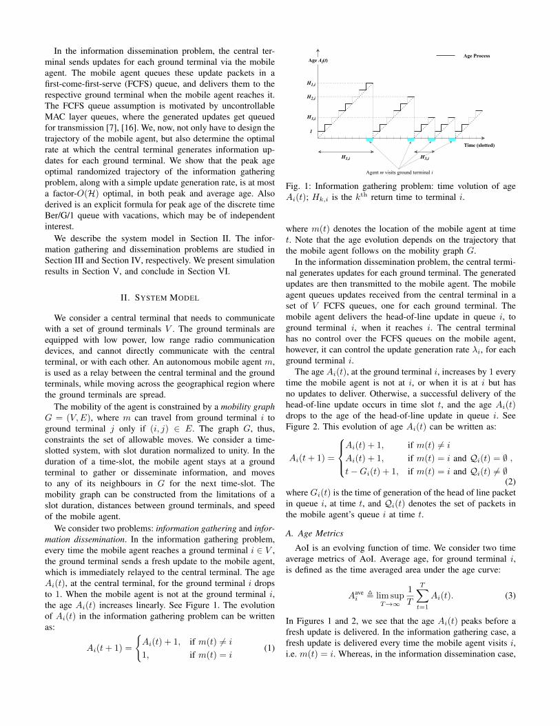
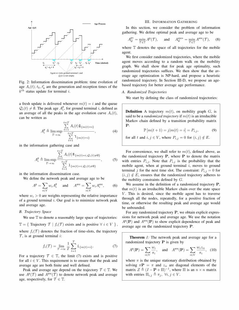
We consider two problems: information gathering and infor-mation dissemination. In the information gathering problem,every time the mobile agent reaches a ground terminal i ∈ V ,the ground terminal sends a fresh update to the mobile agent,which is immediately relayed to the central terminal. The ageAi(t), at the central terminal, for the ground terminal i dropsto 1. When the mobile agent is not at the ground terminal i,the age Ai(t) increases linearly. See Figure 1. The evolutionof Ai(t) in the information gathering problem can be writtenas:

Ai(t+ 1) =

{Ai(t) + 1, if m(t) 6= i

1, if m(t) = i(1)

Time (slotted)

Age Process

H1,i H3,i

1 

H1,i

H3,i

H2,i

Agent m visits ground terminal i

Age Ai(t)

Fig. 1: Information gathering problem: time volution of ageAi(t); Hk,i is the kth return time to terminal i.

where m(t) denotes the location of the mobile agent at timet. Note that the age evolution depends on the trajectory thatthe mobile agent follows on the mobility graph G.

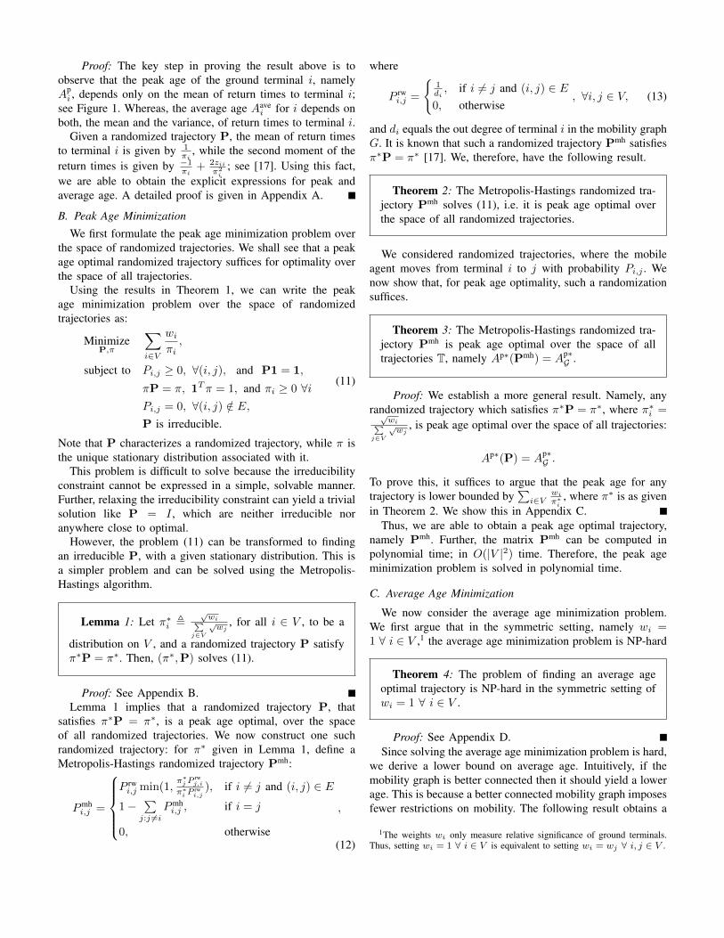
In the information dissemination problem, the central termi-nal generates updates for each ground terminal. The generatedupdates are then transmitted to the mobile agent. The mobileagent queues updates received from the central terminal in aset of V FCFS queues, one for each ground terminal. Themobile agent delivers the head-of-line update in queue i, toground terminal i, when it reaches i. The central terminalhas no control over the FCFS queues on the mobile agent,however, it can control the update generation rate λi, for eachground terminal i.

The age Ai(t), at the ground terminal i, increases by 1 everytime the mobile agent is not at i, or when it is at i but hasno updates to deliver. Otherwise, a successful delivery of thehead-of-line update occurs in time slot t, and the age Ai(t)drops to the age of the head-of-line update in queue i. SeeFigure 2. This evolution of age Ai(t) can be written as:

Ai(t+ 1) =

Ai(t) + 1, if m(t) 6= i

Ai(t) + 1, if m(t) = i and Qi(t) = ∅t−Gi(t) + 1, if m(t) = i and Qi(t) 6= ∅

,

(2)where Gi(t) is the time of generation of the head of line packetin queue i, at time t, and Qi(t) denotes the set of packets inthe mobile agent’s queue i at time t.

A. Age Metrics

AoI is an evolving function of time. We consider two timeaverage metrics of AoI. Average age, for ground terminal i,is defined as the time averaged area under the age curve:

Aavei , lim sup

T→∞

1

T

T∑t=1

Ai(t). (3)

In Figures 1 and 2, we see that the age Ai(t) peaks before afresh update is delivered. In the information gathering case, afresh update is delivered every time the mobile agent visits i,i.e. m(t) = i. Whereas, in the information dissemination case,

t1'

Age Ai(t)

Time (slotted)

Age Process

t1 t2 t2' t3 t3' t4 t4'

t1' ­ t1 + 1

Agent m visits ground terminal i andQi(t) is not empty

t3' ­ t3 + 1

Fig. 2: Information dissemination problem: time evolution ofage Ai(t); tk, t′k are the generation and reception times of thekth status update for terminal i.

a fresh update is delivered whenever m(t) = i and the queueQi(t) 6= ∅. The peak age Ap

i , for ground terminal i, defined asan average of all the peaks in the age evolution curve Ai(t),can be written as

Api , lim sup

T→∞

t=T∑t=1

Ai(t)1{m(t)=i}

t=T∑t=1

1{m(t)=i}

, (4)

in the information gathering case and

Api , lim sup

T→∞

t=T∑t=1

Ai(t)1{m(t)=i,Qi(t)6=∅}

t=T∑t=1

1{m(t)=i,Qi(t) 6=∅}

, (5)

in the information dissemination case.We define the network peak and average age to be

Ap =∑i∈V

wiApi and Aave =

∑i∈V

wiAavei , (6)

where wi > 0 are weights representing the relative importanceof a ground terminal i. Our goal is to minimize network peakand average age.

B. Trajectory SpaceWe use T to denote a reasonably large space of trajectories:

T = { Trajectory T | fi(T ) exists and is positive ∀ i ∈ V } ,

where fi(T ) denotes the fraction of time-slots, the trajectoryT , is at ground terminal i:

fi(T ) = limT→∞

1

T

T∑t=1

1{m(t)=i}. (7)

For a trajectory T ∈ T, the limit (7) exists and is positivefor all i ∈ V . This requirement is to ensure that the peak andaverage age are both finite and well defined.

Peak and average age depend on the trajectory T ∈ T. Weuse Ap(T ) and Aave(T ) to denote network peak and averageage, respectively, for T ∈ T.

III. INFORMATION GATHERING

In this section, we consider the problem of informationgathering. We define optimal peak and average age to be

Ap∗G = min

T ∈TAp(T ), and Aave∗

G = minT ∈T

Aave(T ), (8)

where T denotes the space of all trajectories for the mobileagent.

We first consider randomized trajectories, where the mobileagent moves according to a random walk on the mobilitygraph. We shall show that for peak age optimality, suchrandomized trajectories suffices. We then show that the av-erage age optimization is NP-hard, and propose a heuristicrandomized trajectory. In Section III-D, we propose an age-based trajectory for better average age performance.

A. Randomized Trajectories

We start by defining the class of randomized trajectories:

Definition A trajectory m(t), on mobility graph G, issaid to be a randomized trajectory if m(t) is an irreducibleMarkov chain defined by a transition probability matrixP:

P [m(t+ 1) = j|m(t) = i] = Pi,j , (9)

for all t and i, j ∈ V , where Pi,j = 0 for (i, j) /∈ E.

For convenience, we shall refer to m(t), defined above, asthe randomized trajectory P, where P to denote the matrixwith entries Pi,j . Note that Pi,j is the probability that themobile agent, when at ground terminal i, moves to groundterminal j for the next time slot. The constraint: Pi,j = 0 for(i, j) /∈ E, ensures that the randomized trajectory adheres tothe mobility constraints defined by G.

We assume in the definition of a randomized trajectory P,that m(t) is an irreducible Markov chain over the state spaceV . This is desired, since the mobile agent has to traversethrough all the nodes, repeatedly, for a positive fraction oftime, or otherwise the resulting peak and average age wouldbe unbounded.

For any randomized trajectory P, we obtain explicit expres-sions for network peak and average age. We use the notationAp(P) and Aave(P) to show explicit dependence of peak andaverage age on the randomized trajectory P.

Theorem 1: The network peak and average age for arandomized trajectory P is given by

Ap(P) =∑i∈V

wiπi, and Aave(P) =

∑i∈V

wiziiπi

, (10)

where π is the unique stationary distribution obtained bysolving πP = π and zii are diagonal elements of thematrix Z , (I −P + Π)−1, where Π is an n× n matrixwith entries Πi,j , πj , ∀i, j ∈ V .

Proof: The key step in proving the result above is toobserve that the peak age of the ground terminal i, namelyApi , depends only on the mean of return times to terminal i;

see Figure 1. Whereas, the average age Aavei for i depends on

both, the mean and the variance, of return times to terminal i.Given a randomized trajectory P, the mean of return times

to terminal i is given by 1πi

, while the second moment of thereturn times is given by −1πi

+ 2ziiπ2i

; see [17]. Using this fact,we are able to obtain the explicit expressions for peak andaverage age. A detailed proof is given in Appendix A.

B. Peak Age Minimization

We first formulate the peak age minimization problem overthe space of randomized trajectories. We shall see that a peakage optimal randomized trajectory suffices for optimality overthe space of all trajectories.

Using the results in Theorem 1, we can write the peakage minimization problem over the space of randomizedtrajectories as:

MinimizeP,π

∑i∈V

wiπi,

subject to Pi,j ≥ 0, ∀(i, j), and P1 = 1,

πP = π, 1Tπ = 1, and πi ≥ 0 ∀iPi,j = 0, ∀(i, j) /∈ E,P is irreducible.

(11)

Note that P characterizes a randomized trajectory, while π isthe unique stationary distribution associated with it.

This problem is difficult to solve because the irreducibilityconstraint cannot be expressed in a simple, solvable manner.Further, relaxing the irreducibility constraint can yield a trivialsolution like P = I , which are neither irreducible noranywhere close to optimal.

However, the problem (11) can be transformed to findingan irreducible P, with a given stationary distribution. This isa simpler problem and can be solved using the Metropolis-Hastings algorithm.

Lemma 1: Let π∗i ,√wi∑

j∈V

√wj

, for all i ∈ V , to be a

distribution on V , and a randomized trajectory P satisfyπ∗P = π∗. Then, (π∗,P) solves (11).

Proof: See Appendix B.Lemma 1 implies that a randomized trajectory P, that

satisfies π∗P = π∗, is a peak age optimal, over the spaceof all randomized trajectories. We now construct one suchrandomized trajectory: for π∗ given in Lemma 1, define aMetropolis-Hastings randomized trajectory Pmh:

Pmhi,j =

P rwi,j min(1,

π∗jPrwj,i

π∗i Prwi,j

), if i 6= j and (i, j) ∈ E1−

∑j:j 6=i

Pmhi,j , if i = j

0, otherwise

,

(12)

where

P rwi,j =

{1di, if i 6= j and (i, j) ∈ E

0, otherwise, ∀i, j ∈ V, (13)

and di equals the out degree of terminal i in the mobility graphG. It is known that such a randomized trajectory Pmh satisfiesπ∗P = π∗ [17]. We, therefore, have the following result.

Theorem 2: The Metropolis-Hastings randomized tra-jectory Pmh solves (11), i.e. it is peak age optimal overthe space of all randomized trajectories.

We considered randomized trajectories, where the mobileagent moves from terminal i to j with probability Pi,j . Wenow show that, for peak age optimality, such a randomizationsuffices.

Theorem 3: The Metropolis-Hastings randomized tra-jectory Pmh is peak age optimal over the space of alltrajectories T, namely Ap∗(Pmh) = Ap∗

G .

Proof: We establish a more general result. Namely, anyrandomized trajectory which satisfies π∗P = π∗, where π∗i =√

wi∑j∈V

√wj

, is peak age optimal over the space of all trajectories:

Ap∗(P) = Ap∗G .

To prove this, it suffices to argue that the peak age for anytrajectory is lower bounded by

∑i∈V

wi

π∗i, where π∗ is as given

in Theorem 2. We show this in Appendix C.Thus, we are able to obtain a peak age optimal trajectory,

namely Pmh. Further, the matrix Pmh can be computed inpolynomial time; in O(|V |2) time. Therefore, the peak ageminimization problem is solved in polynomial time.

C. Average Age Minimization

We now consider the average age minimization problem.We first argue that in the symmetric setting, namely wi =1 ∀ i ∈ V ,1 the average age minimization problem is NP-hard

Theorem 4: The problem of finding an average ageoptimal trajectory is NP-hard in the symmetric setting ofwi = 1 ∀ i ∈ V .

Proof: See Appendix D.Since solving the average age minimization problem is hard,

we derive a lower bound on average age. Intuitively, if themobility graph is better connected then it should yield a lowerage. This is because a better connected mobility graph imposesfewer restrictions on mobility. The following result obtains a

1The weights wi only measure relative significance of ground terminals.Thus, setting wi = 1 ∀ i ∈ V is equivalent to setting wi = wj ∀ i, j ∈ V .

lower bound on network average age by comparing it with thenetwork average age of a complete graph.

Theorem 5: For any trajectory T ∈ T, the networkaverage age is lower bounded by

Aave(T ) ≥ 1

2

∑i∈V

(wiπ∗i

+ wi

), (14)

where π∗i =√wi∑

j∈V√wj

for all i ∈ V .

Proof See Appendix E.

Note that the term∑i∈V

wi

π∗iis nothing but the optimal peak

age Ap∗G ; see Theorem 3. Furthermore, the lower bound in

Theorem 5 is independent of the trajectory T . Therefore, weget

Aave∗G = min

T ∈TAave(T ) ≥ Aave

LB =1

2Ap∗G +

1

2

∑i∈V

wi, (15)

where T is the space of all trajectories. It must be noted that asimilar result was derived in the case of link scheduling for ageminimization in [7]. The similarity of the result is rooted inthe fact that the information gathering problem in the completegraph case is equivalent to the link scheduling problem in [7],in which at most one link can be activated simultaneously.

1) A Heuristic Randomized Trajectory: Motivated by thepeak age optimality results of the previous section, we restrictourselves to the space of randomized trajectories, and proposea heuristic, called the fastest-mixing randomized trajectory,and prove an average age performance bound for it.

Using the results in Theorem 1, the average age minimiza-tion problem over the space of randomized trajectories can bewritten as

MinimizeP,π,Z

∑i∈V

wiziiπi

,

subject to Pi,j ≥ 0, ∀ (i, j), and P1 = 1,

πP = π, 1Tπ = 1, and πi ≥ 0 ∀iPi,j = 0, ∀(i, j) /∈ E,P is irreducible,Πi,j = πj ∀ (i, j),

Z = (I −P + Π)−1.

(16)

Here, P is the randomized trajectory and π the uniquestationary distribution corresponding to P. Solving (16) canbe computationally complex. Not only do we have the ir-reducibility constraint, but also a non-linear constraint inZ = (I −P + Π)−1.

We next upper bound the network average age, for anyrandomized trajectory P of the mobile agent. We first definemixing time for a randomized trajectory.

To do this, we first discuss the notion of stopping rules andstopping times in a Markov chain. A stopping rule is a rulethat observes the walk on a Markov chain and, at each step,

decides whether or not to stop the walk based on the walkso far. Stopping rules can make probabilistic decisions andtherefore the time at which the walk stops, called the stoppingtime, is a random variable.

Mixing Time [18] The hitting time from state distribution σ1to σ2 on a Markov chain is the minimum expected stoppingtime over all stopping rules that, beginning at σ1, stop in theexact distribution of σ2. In other words, it is the expectednumber of steps that the optimal stopping rule takes to movefrom σ1 to σ2. This is denoted by H(σ1, σ2). The mixing timeH of a Markov chain P is then defined as

H , supσ∈∆(V )

H(σ, π), (17)

where ∆(V ) is the collection of all distributions on V andπ is the stationary distribution of P. In other words, it is theexpected time taken to reach stationarity using the optimalstopping rule and starting at the worst initial distribution.

Lemma 2: The network average age for a randomizedtrajectory P is upper bounded by

Aave(P) =∑i∈V

wiziiπi≤ 4HAp(P) +

∑i∈V

wi, (18)

where H denotes the mixing time of the randomizedtrajectory P.

Proof: First, we define the quantityZ , max

i

∑j

|zij − πj |, called the discrepancy of the

randomized trajectory P. This definition implies thatzii ≤ Z + πi, ∀i ∈ V. Thus, we get the following upperbound: ∑

i∈V

wiziiπi≤∑i∈V

(wiZπi

+ wi

). (19)

However, from [19] we know that Z ≤ 4H, where H is themixing time of the randomized trajectory P. Thus, we havethe required result∑

i∈V

wiziiπi≤∑i∈V

(4wiHπi

+ wi

)= 4HAp(P) +

∑i∈V

wi,

where the last equality follows from Theorem 1.We use this relation and suggest the following heuristic forminimizing age: Find the fastest mixing randomized trajectoryP on the mobility graph G that minimizes peak age.

From the proof of Theorem 3, we know that for a ran-domized trajectory P to be peak age optimal all we needis πi ∝

√wi, where π is the stationary distribution of P.

It, therefore, suffices to find P that satisfies πi ∝√wi, and

simultaneously minimizes the mixing time H. We call this thefastest-mixing randomized trajectory, and use P∗ to denote it.The following result provides a way to obtain P∗ by solvinga convex program.

Theorem 6: The fastest mixing randomized trajectorycan be found by solving the following convex optimiza-tion problem:

MinimizeP

µ(P) = ||P−Π∗||2,

subject to Pi,j ≥ 0, ∀(i, j),P1 = 1,

π∗P = π∗, Π∗i,j = π∗i ∀ i, j ∈ V,Pi,j = 0,∀(i, j) /∈ E.

(20)

Here ||A||2 denotes the spectral norm of matrix A andπ∗i =

√wi∑

j∈V√wj, ∀i ∈ V .

Proof: See Appendix F.This convex program (20) finds a randomized trajectory P

on G that is closest to the stationary randomized walk Π∗, inthe spectral norm sense. Also, P ∗ is peak age optimal on graphG, since it satisfies π∗i ∝

√wi. Note that, the problem (20)

can be solved in polynomial time by converting it to a semi-definite program [20].

We now bound the average age performance of the fastest-mixing randomized trajectory.

Theorem 7: The network average age of the fastest-mixing randomized trajectory is at most 8H-factor awayfrom the optimal average age:

Aave(P∗)

Aave∗G

≤ 8H, (21)

where H is the mixing time of P ∗.

Proof See Appendix G.

To see the usefulness of the fastest-mixing randomized tra-jectory, and Theorem 7, consider a random geometric graphG(n, r). The graph consists of n nodes spread over a unitsquare with a link between every two nodes that are within adistance r. If v is the physical speed of the mobile agent, thenr must equal vτ , where τ is the slot duration. We know thatmixing time of G(n, r) is O

(lognr2

), and therefore, the fastest-

mixing randomized trajectory would be at most O(

lognv2maxτ

2

)factor optimal. For highly connected graphs, such as Diracgraphs in which the degree of each node is at least |V |/2, wehave constant factor of optimality; since the mixing times areO(1). [21] establishes a connection between the existence oflong paths in graphs and their mixing times.

D. Age-based Trajectories

In the last two sub-sections, we proposed two randomizedtrajectories, namely Pmh and P∗. Both were peak age optimal,while the latter was also factor-H average age optimal. Wealso noted that solving the average age problem is generally

1

2 3

4 5 6 7

Fig. 3: Mobility graph restricted to a binary tree.

hard. We now propose an age-based trajectory which can beconstant factor age optimal.

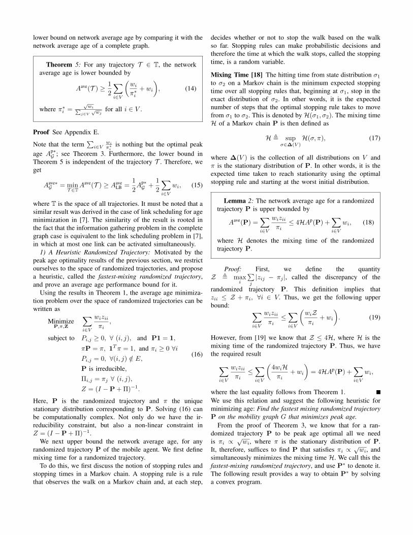
Age-based trajectory In every time slot, agent m movesto the location that has the highest weighted function ofAi(t). Specifically, if m(t) = i then

m(t+ 1) = arg maxj:(i,j)∈E

wjg (Aj(t)) , (22)

for all i, j ∈ V and time t, where g(·) is an increasingfunction.

In the symmetric setting, where wi = 1 ∀ i ∈ V , we observethat the age-based trajectory is a repeated depth-first traversalof the mobility graph G. This can be verified easily when themobility graph is a tree. Consider the tree in Figure 3, andassume that we start at the root node 1. The trajectory of theagent following the rule described above would be 1→ 2→4→ 2→ 5→ 2→ 1→ 3→ 6→ 3→ 7→ 3→ 1... This isprecisely the depth-first traversal of the tree graph.

In the symmetric setting, where wi = 1 ∀ i ∈ V , we nowprove that the age-based trajectory is factor-2 optimal.

Theorem 8: In the symmetric setting wi = 1 ∀ i ∈ V ,the network average age Aave for the age-based trajectoryis bounded by

Aave

Aave∗G≤ 2|V |+ 1

|V |+ 1≤ 2, (23)

for any increasing function g(·).

Proof: See Appendix HThis age-based policy can be implemented in an online

fashion if the mobile agent has access to age Ai(t) of theneighboring terminals. The complexity of implementing thistrajectory is then at most linear in the time-horizon and |V |.

IV. INFORMATION DISSEMINATION

We now consider the information dissemination problem.The central terminal generates updates for every ground ter-minal i, at rate λi, according to a Bernoulli process. Thegenerated updates for the ground terminal i are sent to themobile agent, which get queued in the ith FCFS queue. Themobile agent follows a trajectory T , and delivers the head-of-line update in queue i to terminal i, when it reaches it.

Our objective is to minimize the network peak age andaverage age over the space of update generation rates λ andall trajectories T:

Ap∗D = min

T ∈T,λ

∑i∈V

wiApi , and Aave∗

D = minT ∈T,λ

∑i∈V

wiAavei ,

(24)where Ap

i denotes peak age and Aavei denotes the average age

of terminal i. Their evolution is given by (2). For convenience,we have omitted their explicit dependence on T ∈ T and λ.

Motivated by the results for the information gatheringproblem, we consider randomized trajectories. Note that anarriving update in queue i has service time equal to the inter-visit times to ground terminal i, provided the update arrivedwhen the queue i was not-empty; Qi(t) 6= ∅. However, whenan update arrives to an empty queue i, the time to deliveryis not the inter-visit time, and depends on the location of themobile agent at the time of arrival.

Since the analysis of age for such a queueing system maybe difficult, we provide an upper bound, by comparing the theith queue with a discrete time Ber/G/1 queue with vacations:whenever the ith queue is empty pretend that it goes on avacation, with vacation times having the same distribution asinter-visit time; otherwise the service times for the queue arejust inter-visit times. Clearly, the age process of such a FCFSqueue is an upper bound for the age process Ai(t). Thus, weupper bound the peak age Ap

i and average age Aavei , by the

peak and average age of this Ber/G/1 queue with vacations.We first analyze peak and average age of a Ber/G/1 queuewith vacations.

A. Age for Ber/G/1 Queue with Vacations

Consider a discrete time FCFS Ber/G/1 queue with vaca-tions, where an arrival occurs with probability λ, the servicetimes S are generally distributed with mean E [S] = 1/µ, andthe vacation times V are also generally distributed.

We obtain an expression for the peak age of a discrete timeBer/G/1 queue with vacations, and a bound on average age.

Lemma 3: The peak age for a discrete time FCFSBer/G/1 queue with vacations is given by

Ap =1

λ+

1

µ+λE[S2]− ρ

2(1− ρ)+

E[V 2]

2E [V ]− 1

2, (25)

where ρ = λµ , while the average age is upper-bounded by

peak age, namely Aave ≤ Ap.

Proof: The peak age for a FCFS queue is given by

Ap = E [T +X] , (26)

where T denotes the time an update spends in the queueand X is the inter-arrival time between two updates. Giventhat vacation times are distributed i.i.d according to randomvariable V , we have

E[T ] =λE[S2]− ρ

2(1− ρ)+

1

µ+

E[V 2]

2E [V ]− 1

2, (27)

where S denotes the service time distribution. Substitutingthis and E [X] = 1

λ in (26), we obtain the expression forpeak age. For the derivation of average system time E [T ],see Appendix I.

The upper-bound on average age directly follows from theobservation that total time spent in the queue is negativelycorrelated with inter-arrival times. For details, see Appendix I.

B. Age Minimization Problem

Using Lemma 3, we now obtain an upper-bound on both,network peak and average age, for a given randomized trajec-tory P and update generation rates λ.

Lemma 4: For a randomized trajectory P and packetgeneration rates λ, the peak and average age for a groundterminal i is upper-bounded by

AUBi =

1

πi

[1 + zii +

1

ρi+

ziiρi1− ρi

]− ρi

1− ρi− 1, (28)

for all i ∈ V , where π is the unique stationary distributionof P, Z = (I − P + Π)−1, Π is a matrix with all rowsequal to the stationary distribution vector π, and ρi , λi

πi.

Proof: See Appendix J.We propose a policy, i.e. a randomized trajectory P and

update generation rate λ, that minimizes the age upper-boundAUB =

∑i∈V wiA

UBi :

Definition Separation Principle Policy1) Mobile agent follows the randomized trajectory P∗

obtained by solving (20).2) Generate updates for the ground terminal i at rate

λ∗i =π∗i

1 +√z∗ii − π∗i

, (29)

where π∗i =√wi∑

j∈V wjand zii are diagonal elements

of the matrix Z = (I −P∗ + Π∗)−1.

We call it the separation principle policy for two reasons.Firstly, P∗ is the fastest-mixing randomized trajectory, whichwe proposed for minimizing average age in the informationgathering problem. Secondly, the update generation rate forthe ground terminal i, depends only on zii and πi, which arefunctions of the first and second moments of the return timesto terminal i under trajectory P∗:

E [Hi] =1

πiand E

[H2i

]= − 1

πi+

2ziiπi

,

where Hi denotes the return time to terminal i, starting fromi, under the fastest mixing randomized trajectory P∗. We nowbound the performance of this separation principle policy.

Theorem 9: The peak and average age of the separationprinciple policy is bounded by

Ap

Ap∗D≤ 4H+ 4

√H+ 2 and

Aave

Aave∗D≤ 8H+ 8

√H+ 4,

where H is the mixing time of the randomized trajectoryP∗.

Proof: See Appendix K.The separation principle policy is factor O(H) peak age and

average age optimal. It is worthwhile to note that a similarseparation principle policy was established in a completelydifferent setting of scheduling links for age minimizationin [7]. Theorem 9 generalizes that result to a graph.

V. SIMULATION RESULTS

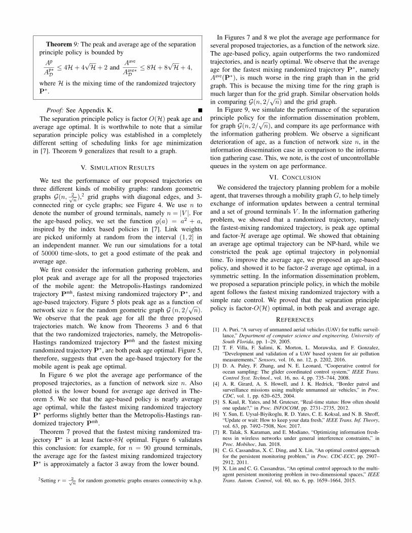
We test the performance of our proposed trajectories onthree different kinds of mobility graphs: random geometricgraphs G(n, 2√

n),2 grid graphs with diagonal edges, and 3-

connected ring or cycle graphs; see Figure 4. We use n todenote the number of ground terminals, namely n = |V |. Forthe age-based policy, we set the function g(a) = a2 + a,inspired by the index based policies in [7]. Link weightsare picked uniformly at random from the interval (1, 2] inan independent manner. We run our simulations for a totalof 50000 time-slots, to get a good estimate of the peak andaverage age.

We first consider the information gathering problem, andplot peak and average age for all the proposed trajectoriesof the mobile agent: the Metropolis-Hastings randomizedtrajectory Pmh, fastest mixing randomized trajectory P∗, andage-based trajectory. Figure 5 plots peak age as a function ofnetwork size n for the random geometric graph G (n, 2/

√n).

We observe that the peak age for all the three proposedtrajectories match. We know from Theorems 3 and 6 thatthat the two randomized trajectories, namely, the Metropolis-Hastings randomized trajectory Pmh and the fastest mixingrandomized trajectory P∗, are both peak age optimal. Figure 5,therefore, suggests that even the age-based trajectory for themobile agent is peak age optimal.

In Figure 6 we plot the average age performance of theproposed trajectories, as a function of network size n. Alsoplotted is the lower bound for average age derived in The-orem 5. We see that the age-based policy is nearly averageage optimal, while the fastest mixing randomized trajectoryP∗ performs slightly better than the Metropolis-Hastings ran-domized trajectory Pmh.

Theorem 7 proved that the fastest mixing randomized tra-jectory P∗ is at least factor-8H optimal. Figure 6 validatesthis conclusion: for example, for n = 90 ground terminals,the average age for the fastest mixing randomized trajectoryP∗ is approximately a factor 3 away from the lower bound.

2Setting r = 2√n

for random geometric graphs ensures connectivity w.h.p.

In Figures 7 and 8 we plot the average age performance forseveral proposed trajectories, as a function of the network size.The age-based policy, again outperforms the two randomizedtrajectories, and is nearly optimal. We observe that the averageage for the fastest mixing randomized trajectory P∗, namelyAave(P∗), is much worse in the ring graph than in the gridgraph. This is because the mixing time for the ring graph ismuch larger than for the grid graph. Similar observation holdsin comparing G(n, 2/

√n) and the grid graph.

In Figure 9, we simulate the performance of the separationprinciple policy for the information dissemination problem,for graph G(n, 2/

√n), and compare its age performance with

the information gathering problem. We observe a significantdeterioration of age, as a function of network size n, in theinformation dissemination case in comparison to the informa-tion gathering case. This, we note, is the cost of uncontrollablequeues in the system on age performance.

VI. CONCLUSION

We considered the trajectory planning problem for a mobileagent, that traverses through a mobility graph G, to help timelyexchange of information updates between a central terminaland a set of ground terminals V . In the information gatheringproblem, we showed that a randomized trajectory, namelythe fastest-mixing randomized trajectory, is peak age optimaland factor-H average age optimal. We showed that obtainingan average age optimal trajectory can be NP-hard, while weconstricted the peak age optimal trajectory in polynomialtime. To improve the average age, we proposed an age-basedpolicy, and showed it to be factor-2 average age optimal, in asymmetric setting. In the information dissemination problem,we proposed a separation principle policy, in which the mobileagent follows the fastest mixing randomized trajectory with asimple rate control. We proved that the separation principlepolicy is factor-O(H) optimal, in both peak and average age.

REFERENCES

[1] A. Puri, “A survey of unmanned aerial vehicles (UAV) for traffic surveil-lance,” Department of computer science and engineering, University ofSouth Florida, pp. 1–29, 2005.

[2] T. F. Villa, F. Salimi, K. Morton, L. Morawska, and F. Gonzalez,“Development and validation of a UAV based system for air pollutionmeasurements,” Sensors, vol. 16, no. 12, p. 2202, 2016.

[3] D. A. Paley, F. Zhang, and N. E. Leonard, “Cooperative control forocean sampling: The glider coordinated control system,” IEEE Trans.Control Syst. Technol., vol. 16, no. 4, pp. 735–744, 2008.

[4] A. R. Girard, A. S. Howell, and J. K. Hedrick, “Border patrol andsurveillance missions using multiple unmanned air vehicles,” in Proc.CDC, vol. 1, pp. 620–625, 2004.

[5] S. Kaul, R. Yates, and M. Gruteser, “Real-time status: How often shouldone update?,” in Proc. INFOCOM, pp. 2731–2735, 2012.

[6] Y. Sun, E. Uysal-Biyikoglu, R. D. Yates, C. E. Koksal, and N. B. Shroff,“Update or wait: How to keep your data fresh,” IEEE Trans. Inf. Theory,vol. 63, pp. 7492–7508, Nov. 2017.

[7] R. Talak, S. Karaman, and E. Modiano, “Optimizing information fresh-ness in wireless networks under general interference constraints,” inProc. Mobihoc, Jun. 2018.

[8] C. G. Cassandras, X. C. Ding, and X. Lin, “An optimal control approachfor the persistent monitoring problem,” in Proc. CDC-ECC, pp. 2907–2912, 2011.

[9] X. Lin and C. G. Cassandras, “An optimal control approach to the multi-agent persistent monitoring problem in two-dimensional spaces,” IEEETrans. Autom. Control, vol. 60, no. 6, pp. 1659–1664, 2015.

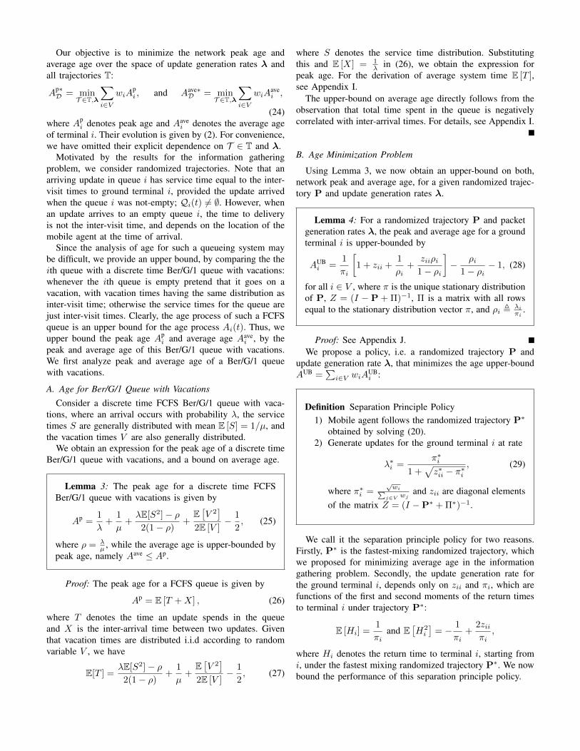
(a) (b) (c)

Fig. 4: (a) A random geometric graph with 100 nodes, (b) A grid graph with 81 nodes and diagonal edges, and (c) A 3-connectedring or cycle graph with 21 nodes.

10 20 30 40 50 60 70 80 9010

20

30

40

50

60

70

80

90

Network Size n

Netw

ork

Pea

k A

ge A

p/n

Metropolis−Hastings Pmh

Fastest Mixing P*

Age−Based

Optimal Peak Age

Fig. 5: Information gathering problem in G(n, 2/√n): network

peak age as a function of network size n for several proposedtrajectories of the mobile agent.

10 20 30 40 50 60 70 80 900

20

40

60

80

100

120

140

160

180

Network Size n

Netw

ork

Average A

ge A

ave /n

Metropolis−Hastings Pmh

Fastest Mixing P*

Age−Based

Lower Bound

Fig. 6: Information gathering problem in G(n, 2/√n): network

average age as a function of network size n for severalproposed trajectories of the mobile agent.

20 40 60 80 100 1200

50

100

150

200

250

Network Size n

Netw

ork

Av

erag

e A

ge A

ave /n

Metropolis−Hastings Pmh

Fastest Mixing P*

Age−Based

Lower Bound

Fig. 7: Information gathering problem in the Grid graph:network average age as a function of network size n for severalproposed trajectories of the mobile agent.

10 20 30 40 50 60 70 80 900

50

100

150

200

250

300

350

400

Network Size n

Netw

ork

Av

era

ge A

ge A

av

e /n

Metropolis−Hastings Pmh

Fastest Mixing P*

Age−Based

Lower Bound

Fig. 8: Information gathering problem in the Ring graph:network average age as a function of network size n for severalproposed trajectories of the mobile agent.

10 20 30 40 50 60 70 80 900

100

200

300

400

500

600

Network size n

Netw

ork

Av

era

ge A

ge A

av

e /n

Info. Diss. − Sep. Principle Policy P*,λ*

Info. Gathering − Fastest Mixing P*

Lower Bound

Fig. 9: Network average age as a function of network size n.

[10] S. L. Smith, M. Schwager, and D. Rus, “Persistent monitoring ofchanging environments using a robot with limited range sensing,” inProc. ICRA, pp. 5448–5455, 2011.

[11] G. D. Celik and E. Modiano, “Dynamic vehicle routing for datagathering in wireless networks,” in Proc. CDC, pp. 2372–2377, 2010.

[12] D. Ciullo, G. D. Celik, and E. Modiano, “Minimizing transmissionenergy in sensor networks via trajectory control,” in Proc. WiOpt,pp. 132–141, 2010.

[13] S. Alamdari, E. Fata, and S. L. Smith, “Min-max latency walks:Approximation algorithms for monitoring vertex-weighted graphs,” inAlgorithmic Foundations of Robotics X, pp. 139–155, Springer, 2013.

[14] S. Alamdari, E. Fata, and S. L. Smith, “Persistent monitoring in discreteenvironments: Minimizing the maximum weighted latency betweenobservations,” The International Journal of Robotics Research, vol. 33,no. 1, pp. 138–154, 2014.

[15] J. Liu, X. Wang, B. Bai, and H. Dai, “Age-optimal trajectory planning forUAV-assisted data collection,” arXiv preprint arXiv:1804.09356, 2018.

[16] S. Kaul, M. Gruteser, V. Rai, and J. Kenney, “Minimizing age ofinformation in vehicular networks,” in Proc. SECON, pp. 350–358, Jun.2011.

[17] D. Aldous and J. Fill, “Reversible markov chains and random walks ongraphs,” 2002.

[18] J. King, “Conductance and rapidly mixing markov chains,” TechnicalReport, University of Waterloo, Mar. 2003.

[19] N. Ailon, S. Chien, and C. Dwork, “On clusters in markov chains,”in Latin American Symposium on Theoretical Informatics, pp. 43–55,Springer, 2006.

[20] S. Boyd, P. Diaconis, and L. Xiao, “Fastest mixing markov chain on agraph,” SIAM Review, vol. 46, no. 4, pp. 667–689, 2004.

[21] I. Pak, “Mixing time and long paths in graphs,” vol. 6, no. 08, pp. 321–328, 2002.

[22] D. P. Bertsekas and R. G. Gallager, Data Networks. Prentice Hall, 2 ed.,1992.

APPENDIX

A. Proof of Theorem 1

Let Api be the peak age for ground terminal i. We defineHk,i to be the kth return time to ground terminal i. Then, thekth age peak for Ai(t) has a value of Hk,i. Let K be thetotal number of returns to i over a time-horizon T . Then, theexpected peak age of ground terminal i is given by

Api = limT→∞

E

[ t=T∑t=1

Ai(t)1{m(t)=i}

t=T∑t=1

1{m(t)=i}

]= limK→∞

E[

1

K

t=K∑k=1

Hk,i

].

(30)

Note that return times to a ground terminal i are i.i.d.random variables given a randomized trajectory P. So, wecan use the law of large numbers to get

Api = E[H1,i] =1

πi, (31)

where πi is the stationary distribution for Markov chain P.The last equality follows from the fact that the expected returntime to a state i for an irreducible Markov chain is given bythe inverse of its stationary probability. Thus, the network ageis given by

Ap =∑i∈V

wiApi =

∑i∈V

wiπi. (32)

For average age, we define a renewal-reward process usingHk,i as our i.i.d. renewal intervals and sum of age Ai(t) duringeach interval as our reward. Let Tk,i =

∑k−1l=1 Hl,i be the

starting time of the kth renewal. The total reward in betweentwo visits to ground terminal i is the sum of the ith age processAi(t) across all time-slots during that interval.

Note that, for the kth renewal interval, Ai(t) grows from1 to Hk,i over the Hk,i time-slots. Thus, the total reward forthe kth renewal interval is given by -

t=Tk,i+Hk,i∑t=Tk,i

Ai(t) =

Hk,i∑a=1

a =H2k,i +Hk,i

2. (33)

Note that this reward is also i.i.d. across renewals as it dependsonly on Hk,i. Thus, by application of the elementary renewaltheorem for renewal-reward processes we get

Aavei = lim

T→∞E[

1

T

t=T∑t=1

Ai(t)

]=

E[H21,i +H1,i]

2E[H1,i]. (34)

For irreducible Markov chains, we know the following resultshold [17]:

E[H1,i] =1

πi,∀i ∈ V and (35)

E[H21,i] =

−1

πi+

2ziiπ2i

, (36)

for all i ∈ V , where zii is the ith diagonal element of thematrix Z = (I − P + Π)−1, with Π being a matrix in whichall rows are the stationary distribution vector π: Πi,j = πj forall i, j ∈ V .

Substituting (35) and (36) in (34), we get

Aavei =

ziiπi, (37)

for all i ∈ V , and therefore,

Aave =∑i∈V

wiAavei =

∑i∈V

wiziiπi

. (38)

B. Proof of Theorem 2

Suppose we could choose any stationary distribution π onV . Then to minimize the network peak age, we would needto solve the following optimization problem

Minimizeπ

∑i∈V

wiπi,

subject to∑i

πi = 1,

πi ≥ 0,∀i ∈ V.

(39)

Using KKT conditions for the optimization problem (39), it isstraightforward to see that

π∗i =

√wi∑

i

√wi,∀i ∈ V. (40)

Clearly, if we could find a randomized trajectory P thatachieves this stationary distribution π∗, then it would be peakage optimal. Thus, any randomized trajectory P that satisfiesπ∗ = π∗P is peak age optimal.

C. Proof of Theorem 3

Let Hk,i to be the kth return time to node i. If K is the totalnumber of returns to ground terminal i over a time horizon T ,then the peak age Ap

i is given by

Api = lim sup

T→∞

t=T∑t=1

Ai(t)1{m(t)=i}

t=T∑t=1

1{m(t)=i}

= lim supK→∞

1

K

k=K∑k=1

Hk,i.

(41)Now, the fraction of time-slots in which the mobile agent isat ground terminal i, is given by

fi = limT→∞

t=T∑t=1

1{m(t)=i}

T= limK→∞

Kk=K∑k=1

Hk,i

=1

Api

, (42)

and therefore, Ap =∑i∈V wiA

pi =

∑i∈V

wi

fi. Note that fi,

being the fraction of time-slots the mobile agent is at terminali, is a distribution over V . Thus, Ap can be lower bounded by

Ap =∑i∈V

wiApi ≥ min

{fi≥0,∑

i fi=1}

∑i∈V

wifi

=∑i∈V

wiπ∗i, (43)

where the last equality is obtained by solving the optimizationproblem, just as in Appendix B.

D. Proof of Theorem 4

To prove NP-hardness, we establish equivalence betweenthe average age minimization problem and the Hamiltoniancycle problem, in the symmetric setting. We know that moreconnected the graph, lower is its network average age. There-fore, the average age for G = (V, E) is lower bounded by theaverage age for the complete graph K(V), given by |V |(|V |+1)

2 .This lower bound can be obtained by using Theorem 5 andsetting wi = 1, ∀i.

If the graph is Hamiltonian, we can achieve this average agelower bound by setting the trajectory equal to a Hamiltoniancycle. This is because in a cyclical trajectory, the agent visitsevery terminal exactly once in every |V | time-slots. Further,if the graph is not Hamiltonian, the optimal average age isstrictly greater than |V |(|V |+1)

2 . This is because in the absenceof a cycle on graph G, the agent cannot visit every terminalexactly once every |V | time-slots. Therefore, if an algorithmwere to solve the average age problem then the same algorithmcould be used to determine whether the graph G is Hamiltonianor not; which is the Hamiltonian cycle problem. Since theHamiltonian cycle problem is NP-complete, the average ageminimization problem must be NP-hard.

E. Proof of Theorem 5

Let Hk,i be the kth return time to ground terminal i, andK be the total number of returns to i over a time-horizon T .Then the average age Aave

i is given by (see Appendix A):

Aavei = lim

T→∞

1

T

t=T∑t=1

Ai(t) = limK→∞

k=K∑k=1

(H2k,i +Hk,i)

2k=K∑k=1

Hk,i

. (44)

Define the empirical first and second moment of return times

be Hi , 1K

k=K∑k=1

Hk,i and H(2)i , 1

K

k=K∑k=1

H2k,i, respectively.

Further, define Vari , H(2)i − H2

i to be the empirical varianceof return times. From (44), we have

Aavei =

1

2+ limK→∞

H(2)i

2Hi

=1

2+ limK→∞

(Hi

)2+ Vari

2Hi

. (45)

Using Cauchy-Schwarz inequality, we can obtain Vari ≥ 0.Applying this to (45), we get

Aavei ≥

1

2+ limK→∞

Hi

2, (46)

Let fi be the fraction of time-slots in which the mobile agentis at ground terminal i. Then,

fi = limT→∞

t=T∑t=1

1{m(t)=i}

T= limK→∞

Kk=K∑k=1

Hk,i

=1

limK→∞ Hi

,

(47)since fi is well defined and positive for all trajectories in T.Substituting (47) in (46) we get Aave

i ≥ 12 + 1

2fi, for all i, and

Aave =∑i∈V

wiAavei ≥

1

2

∑i∈V

wi +1

2

∑i∈V

wifi. (48)

Note that fi, being the fraction of time-slots the mobile agentis at terminal i, is a distribution over V . Thus, the average agein (48) can be lower bounded by

Aave ≥ 1

2

∑i∈V

wi +1

2min

{fi≥0,∑

i fi=1}

∑i∈V

wifi,

=1

2

∑i∈V

wi +1

2

∑i∈V

wiπ∗i,

which proves the result.

F. Proof of Theorem 6

From [20], we know that the fastest mixing, reversibleMarkov chain on a graph G(V,E) having the stationarydistribution π can be found by formulating the followingconvex program:

MinimizeP

||D1/2PD−1/2 − qqT ||2,

subject to Pi,j ≥ 0, ∀(i, j)P1 = 1,

π∗P = PTπ∗,

Pi,j = 0,∀(i, j) /∈ E.

(49)

Here D = diag(π∗) and q = (√π∗1 ,√π∗2 , ...,

√π∗n). Note

that we do not require reversibility, so we can replace thedetailed balance constraint π∗P = PTπ∗ with the globalbalance constraint π∗P = π∗. Also, left and right multiplying(D1/2PD−1/2 − qqT ) by matrices D−1/2 and D1/2, respec-tively, does not change the spectral norm; since P has thesame eigen-values as D1/2PD−1/2 and qqT has the sameeigen-values as D−1/2qqTD1/2 [20]. Further, observe thatD−1/2qqTD1/2 = qqT = Π∗, where Π∗i,j = π∗i ∀ i, j ∈ V.Thus, the optimization problem reduces to (20). This provesthe required result.

G. Proof of Theorem 7

Note that the peak age for the fastest-mixing randomizedtrajectory P∗ is given by Ap(P∗) =

∑i∈V

wi

π∗i, since π∗P∗ =

π∗. From Theorem 5, a lower bound on average age is givenby

AaveLB =

∑i∈V

1

2

(wiπ∗i

+ wi

)=

1

2Ap(P∗) +

1

2

∑i∈V

wi. (50)

To prove the result, it suffuses to argue thatAave(P∗)/ALB ≤ 8H. From (50) and Lemma 2, weget

Aave(P∗)

AaveLB

≤4HAp(P∗) +

∑i∈V wi

12A

p(P∗) + 12

∑i∈V wi

, (51)

≤ 8H, (52)

since H is always greater than or equal to 1.

H. Proof of Theorem 8

The number of steps taken to cover every vertex of a graphby performing a depth first search (DFS) traversal is upperbounded by 2|V |, since every vertex is visited at least onceand the sum total of visits after the first visit to all nodes isat most |V |. This is because every repeated visit to a vertexmeans that at least one new vertex was visited. Thus, everylocation gets visited at least once in every 2|V | time-slots. Thisimplies that the average age of every terminal can be upperbounded by (2|V |+1)

2 .However, from our earlier discussion, we know that the

average age of any terminal is lower bounded by (|V |+1)2 if

all the weights are 1. Combining the upper and lower bounds,we have the required result.

I. Proof of Lemma 3

Derivation of System Time The proof is a discretizedversion of the proof for M/G/1 queues with vacations usingresidual service times as discussed in [22].

Let us define the residual service time for an update attime t, given by R(t), as the amount of time remaining untilthe update currently at the head of the queue is complete,excluding the current time-slot. If the queue is empty, R(t)equals zero.

From [22] we know that the expected waiting time in thequeue can be found using the residual service times as follows

E [TQ] =E [R]

1− ρ, (53)

where ρ = λµ , E [S] = 1

µ and E [R] = limT→∞

E[

1T

t=T∑t=0

R(t)

].

As in [22], E [R] can be computed using a graphical argument.Let service times for the mth packet be Xm, and let the kthvacation time be Vk. Let the total number of packets servedbe M(T ) and the total number of vacations be L(T ), over theentire time-horizon T . Then, we have

1

T

t=T∑t=0

R(t) =1

2

M(T )

T

m=M(T )∑m=1

(X2m −Xm)

M(T )

+1

2

L(T )

T

k=L(T )∑k=1

(V 2k − Vk)

L(T ). (54)

Using the strong law of large numbers and the fact thatM(T )T → λ and L(T )

T → (1−ρ)E[V ] , we get

E [R] =λ(E

[S2]− E [S])

2+

(1− ρ)(E[V 2]− E [V ])

2E [V ].

(55)Combining (53) and (55), we get

E [TQ] =λE[S2]− ρ

2(1− ρ)+

E[V 2]

2E [V ]− 1

2. (56)

The total time spent in the system by a packet is given bythe sum of its waiting time in the queue and its processingtime, which implies

E [T ] = E [S + TQ] =1

µ+λE[S2]− ρ

2(1− ρ)+

E[V 2]

2E [V ]− 1

2, (57)

since E [S] = 1µ .

Average Age: Consider a Ber/G/1 queue with vacationsthat has i.i.d. packet inter-arrival times X1, X2, ... Let Tn bethe total time spent in the system by the nth packet. Then, theaverage age is given by [5]:

Aave =1

λ+ λE[XnTn], (58)

where 1λ = E[Xn]. To evaluate the term E[XnTn], we observe

that larger inter-arrival times Xn between packets mean lesserwait times in the system Tn for individual packets. Thus,Xn and Tn are negatively correlated. Note that for negativelycorrelated random variables the following holds

E [XnTn] ≤ E [Xn]E [Tn] . (59)

This implies

Aave ≤ 1

λ+ λE[Xn]E [Tn] = E [Xn] + E [Tn] = Ap, (60)

since E[Xn] = 1/λ.

J. Proof of Lemma 4Consider a randomized trajectory P and Bernoulli arrival

rates λ = (λ1, λ2, . . .). From the arguments made in Sec-tion IV, we know that the peak age for the ground terminali is upper-bounded by the peak age of a discrete time FCFSBer/G/1 queue with vacations, for which the service timesand vacation times have the same distribution as the inter-visittimes H1,i. Applying Lemma 3 we obtain

Api ≤

1

πi

[1 + zii +

1

ρi+

ziiρi1− ρi

]− ρi

1− ρi−1 , AUB

i , (61)

where we have used the first and second moment of inter-visittimes H1,i [17]:

E[H1,i] =1

πi, E[H2

1,i] =−1

πi+

2ziiπ2i

,∀i ∈ V. (62)

Similarly, we know that the average age for the ground ter-minal i is also upper-bounded by the average age for the FCFSBer/G/1 queue with vacations. Using the fact that Aave ≤ Ap

for the Ber/G/1 queue with vacations (see Lemma 3), we getAavei ≤ AUB

i .

K. Proof of Theorem 9We want to solve the upper bound age minimization prob-

lem, which can be stated as:

MinimizeP,ρ

∑i∈V

wiAUBi ,

subject to Pi,j ≥ 0, ∀(i, j),P1 = 1,

Pi,j = 0, ∀(i, j) /∈ E,P is irreducible.

(63)

We first find the optimal packet generation rates given arandom walk P. Observe that the optimal queue utilizationfactors ρi can be solved for given any fixed irreducible randomwalk P, i.e.

ρ∗i (P) = arg minρi∈[0,1]

AUBi (P, ρi) =

1

1 +√zii − πi

(64)

and

minρi∈[0,1]

AUBi (P, ρi) = AUB

i (P, ρ∗i ) =zii − πi + 2

√zii − πi + 2

πi.

(65)Thus, the upper bound age minimization problem reduces to

MinimizeP

∑i∈V

wi

(zii − πi + 2

√zii − πi + 2

πi

),

subject to Pi,j ≥ 0, ∀(i, j),P1 = 1,

Pi,j = 0, ∀(i, j) /∈ E,P is irreducible.

(66)

Now, we can relate the network age upper bound, given arandom walk P, to its mixing time H. We assume optimalpacket generation rates ρ∗i (P).∑i∈V

wiAUBi (P, ρ∗i (P )) =

∑i∈V

wi

(zii − πi + 2

√zii − πi + 2

πi

),

≤∑i∈V

wi

(Z + 2

√Z + 2

πi

),

≤∑i∈V

wi

(4H+ 4

√H+ 2

πi

),

where inequalities follow from the same argument as in theproof of Lemma 2. Setting P = P∗, we obtain∑

i∈VwiA

UBi (P∗, ρ∗i (P

∗)) ≤∑i∈V

wi

(4H+ 4

√H+ 2

π∗i

),

(67)where H is the mixing time of P ∗. Note that

∑i∈V

wi

π∗iis the

optimal peak age in the information gathering problem, i.e.Ap∗G =

∑i∈V

wi

π∗i. This gives,

AUB(P∗,ρ∗)

Ap∗G

≤ 4H+ 4√H+ 2. (68)

Due to the presence of queues we have Ap∗G ≤ A

p∗D . This, (68),

and the fact that Ap(P∗,ρ∗) ≤ AUB(P∗,ρ∗), yields the peakage bound on the separation principle policy:

Ap(P∗, λ∗)

Ap∗D

≤ 4H+ 4√H+ 2,

since ρ∗ = λ∗.From the discussion following Theorem 5, we know that

2Aave∗G ≥ Ap∗

D . Also, Aave∗G ≤ Aave∗

D and Aave(P∗,ρ∗) ≤AUB(P∗,ρ∗). Combining these with (68) gives us

Aave(P∗, λ∗)

Aave∗D

≤ 8H+ 8√H+ 4, (69)

since ρ∗ = λ∗.