1

Age Optimal Information Gathering andDissemination on Graphs

Vishrant Tripathi, Rajat Talak, and Eytan Modiano, Fellow, IEEE

Abstract—We consider the problem of timely exchange of updates between a central station and a set of ground terminals V , via amobile agent that traverses across the ground terminals along a mobility graph G = (V,E). We design the trajectory of the mobileagent to minimize average-peak and average age of information (AoI), two recently proposed metrics for measuring timeliness ofinformation. We consider randomized trajectories, in which the mobile agent travels from terminal i to terminal j with probability Pi,j .For the information gathering problem, we show that a randomized trajectory is average-peak age optimal and factor-8H average ageoptimal, where H is the mixing time of the randomized trajectory on the mobility graph G. We also show that the average ageminimization problem is NP-hard. For the information dissemination problem, we prove that the same randomized trajectory isfactor-O(H) average-peak and average age optimal. Moreover, we propose an age-based trajectory, which utilizes information aboutcurrent age at terminals, and show that it is factor-2 average age optimal in a symmetric setting.

Index Terms—Age of information, wireless networks, trajectory optimization, scheduling.

F

1 INTRODUCTION

M ANY emerging applications depend on the collection anddelivery of status updates between a set of ground ter-

minals and a central terminal using mobile agents. Examplesinclude: measuring traffic at road intersections [2], temperature,and pollution in cities [3], ocean monitoring using underwaterautonomous vehicles [4], and surveillance using UAVs [5]. Allof these applications depend upon regular status updates, thatare communicated in a timely manner, so as to keep the centralterminal and the ground terminals updated with fresh information.

Age of Information (AoI) is a recently proposed metric thatcaptures timeliness of the received information [6]–[8]. Unlikepacket delay, AoI measures the lag in obtaining information at thedestination node, and is therefore suited for applications involvinggathering or dissemination of time sensitive updates [9]–[11]. Ageof information, at a destination, is defined as the time that elapsedsince the last received information update was generated at thesource. AoI, upon reception of a new update packet, drops to thetime elapsed since generation of the packet, and grows linearlyotherwise. For detailed surveys of AoI literature, see [9] and [12].

We consider the problem of AoI minimization in gatheringand dissemination of information updates, between a set of groundterminals and a central terminal. The information updates can beas small as a single packet containing temperature information or ahigh fidelity image or a video file. The ground terminals representlocations where information of interest is being generated or needsto be delivered. Thus, they could be sensors in a wireless sensornetwork equipped with low power transmitters, where a mobileagent is used for real-time monitoring. Another example is a setof locations that needs timely monitoring via a mobile agent, liketraffic at intersections in a city. A third application consists ofusing a mobile agent to disseminate timely updates in remote

• The authors are with the Laboratory for Information and Decision Sys-tems, Massachusetts Institute of Technology, Cambridge, MA 02139, USA.Email: {vishrant, talak, modiano}@mit.edu.

• A version of this work was presented in IEEE INFOCOM 2019 [1].

Manuscript submitted March 11, 2021.

locations in the event of disasters or an emergency. Further, whilewe discuss the problem in terms of a physical agent and locations,the model can also describe timely monitoring of dynamic contenton the Web using a web-crawler.

We consider two versions of the problem - 1) informationgathering in which ground terminals generate new updates when-ever needed with no queuing; and 2) information dissemination inwhich new updates are generated by a central station accordingto a stochastic process, get queued into FCFS queues and aredelivered to ground terminals.

The age or freshness of information gathered and disseminateddepends on the trajectory of the mobile agent, whose mobility isconstrained to a mobility graph G = (V,E). The mobile agentcan move from ground terminal i to ground terminal j only if(i, j) ∈ E. This model can be used to capture the fact that theagent may not be able to move between any arbitrary locationsdue to topological limitations.

The problem of persistent monitoring in dynamic environ-ments has been considered in [13]–[15] using tools from optimalcontrol. These works focus on minimizing uncertainty whensource locations are time varying, rather than timely monitoringover a fixed set of locations. There is also a large body of workfocused on planning trajectories for a mobile agent to optimizetraditional performance metrics in wireless sensor networks; pri-marily throughput, delay and network lifetime; by leveragingvariants of the Travelling Salesman Problem (TSP) [16]–[20].However, these works do not focus on freshness as a metric.We observe connections to this line of work in our paper, wherewe establish the optimality of a Hamiltonian cycle trajectory in asymmetric setting.

Closer to our work are [21] and [22], in which some ap-proximation trajectories to minimize maximum latency on metricgraphs were proposed. In [23], the authors consider trajectoryplanning for a mobile agent to minimize AoI. They obtain the bestpermutation of nodes for the mobile agent to visit in sequence,given Euclidean distances between the nodes. A similar problemis also considered in [24], where average-peak age minimization

2

for UAV-assisted IoT networks is considered. However, averageage minimization is not considered. In this work, we consider amobile agent gathering/disseminating information from multiplenodes. Its mobility is constrained by a general graph G, andwe seek average-peak and average age optimal trajectories overthe space of all trajectories allowed on this graph G, not justpermutations of nodes. To the best our knowledge, this is the firstwork to consider both average-peak and average AoI minimizationon general mobility graphs G. A preliminary version of this workwas presented in [1].

For the information gathering problem, we design trajectoriesfor the mobile agent to minimize average-peak age and averageage, two popular metrics of AoI. We first consider the spaceof randomized trajectories, in which the mobile agent traversesedges according to a random walk on the mobility graph G. Weshow that a randomized trajectory is in fact average-peak ageoptimal, and that it can be obtained in polynomial time usingthe Metropolis-Hastings algorithm. We then prove that solving forthe average age optimal trajectory is NP-hard, in a symmetricsetting, and propose a heuristic randomized trajectory that issimultaneously average-peak age optimal and factor-8H averageage optimal, where H is the mixing time of the randomizedtrajectory on G. The factor H can scale with the graph size,especially if the graph is not well connected. Thus, we propose anage-based trajectory, in which the mobile agent uses the currentAoI to determine its motion, and show that it is factor-2 optimalin a symmetric setting.

In the information dissemination setting, the mobile agentreceives update packets in separate first-come-first-served (FCFS)queues, one for each terminal. The mobile agent then transmitsthe head-of-line packet from the ith queue when it reaches thelocation of the ith ground terminal. The FCFS queue assumptionis motivated by uncontrollable MAC layer queues, where thegenerated updates get queued for transmission [10], [25]. We, now,not only have to design the trajectory of the mobile agent, but alsodetermine the optimal rate at which the central terminal generatesinformation updates for each ground terminal. We show that theaverage-peak age optimal randomized trajectory for informationgathering, along with a simple update generation rate, is at most afactor-O(H) optimal, in both peak and average age. Also derivedis an explicit formula for average-peak age of the discrete timeBer/G/1 queue with vacations, which may be of independentinterest.

We describe the system model in Section 2. The gathering anddissemination versions are studied in Section 3 and Section 4,respectively. We present simulation results in Section 5, andconclude in Section 6.

2 SYSTEM MODEL

We consider a central terminal that needs to communicate with aset of ground terminals V . The ground terminals are equipped withlow power, low range radio communication devices, and cannotdirectly communicate with the central terminal, or with each other.An autonomous mobile agent m, is used as a relay between thecentral terminal and the ground terminals, while moving acrossthe geographical region where the ground terminals are spread.

The mobility of the agent is constrained by a mobility graphG = (V,E), wherem can travel from ground terminal i to groundterminal j only if (i, j) ∈ E. The graph G, thus, constraints theset of allowable moves. We consider a time-slotted system, with

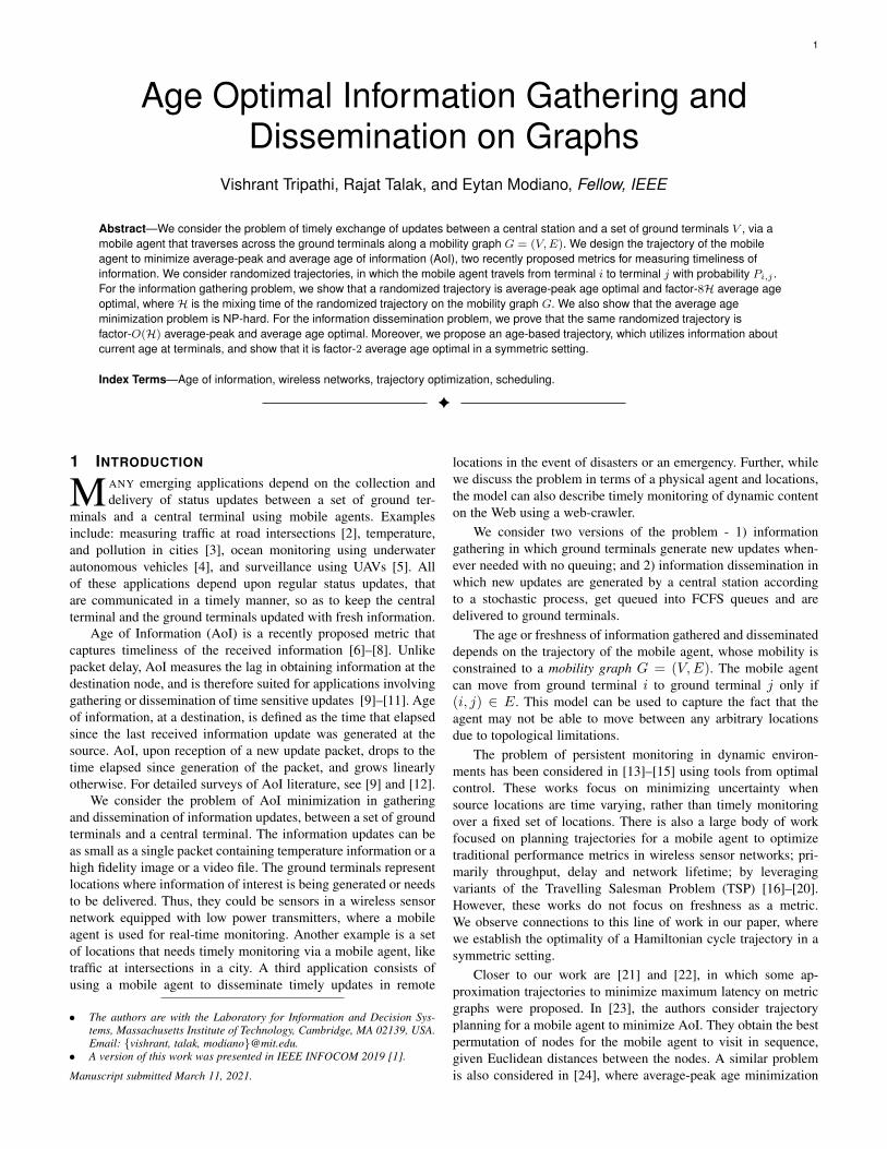
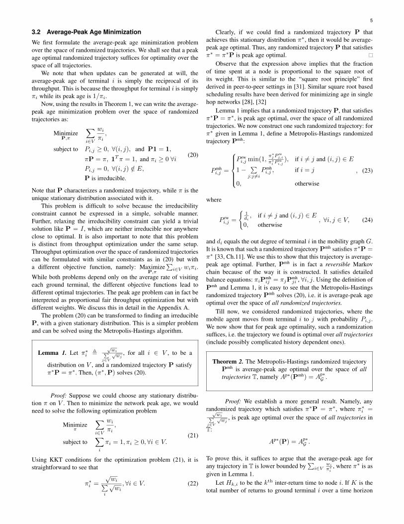
Fig. 1: Information Gathering: time evolution of age Ai(t); Hk,i

is the kth inter-return time to terminal i.

slot duration normalized to unity. In the duration of a time-slot, themobile agent stays at a ground terminal to gather or disseminateinformation, and moves to any of its neighbours in G for thenext time-slot. The mobility graph can be constructed from thelimitations of a slot duration, distances between ground terminals,and speed of the mobile agent. We consider this abstract graphmobility model because of its analytical tractability. This allowsus to gain insight into practical system design and explore thetradeoffs between computational complexity and optimality.

In the information gathering problem, every time the mobileagent reaches a ground terminal i ∈ V , the ground terminal sendsa fresh update to the mobile agent, which is immediately relayedto the central terminal. The age Ai(t), at the central terminal,for the ground terminal i drops to 1. When the mobile agent isnot at the ground terminal i, the age Ai(t) increases linearly. SeeFigure 1. The evolution of Ai(t) in this case can be written as:

Ai(t+ 1) =

{Ai(t) + 1, if m(t) 6= i

1, if m(t) = i(1)

where m(t) denotes the location of the mobile agent at time t.Note that the age evolution depends on the trajectory that themobile agent follows on the mobility graph G.

In the information dissemination setting, the mobile agentreceives updates from a central terminal to be disseminated toeach ground terminal through queues. The mobile agent enqueuesupdates generated stochastically in a set of |V | FCFS queues,one for each ground terminal. It transmits the head-of-line update

3

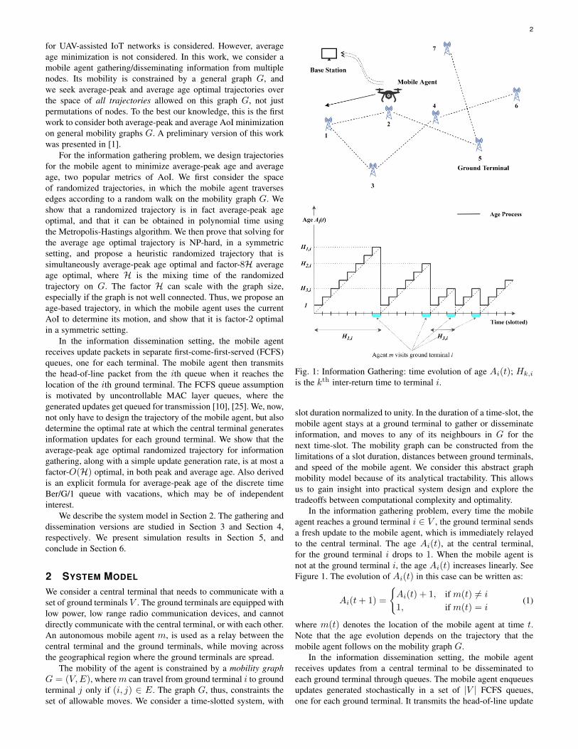
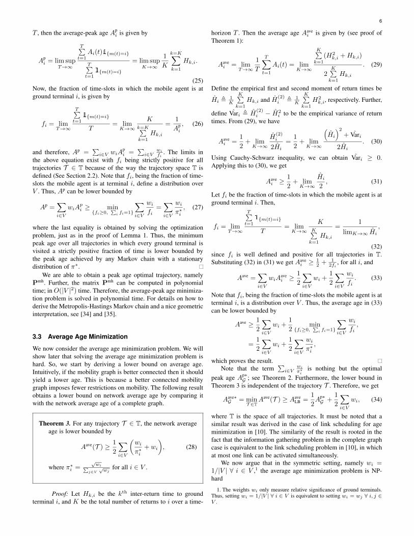
Fig. 2: Information Dissemination: time evolution of age Ai(t);tk, t

′k are the generation and reception times of the kth status

update for terminal i.

in queue i to ground terminal i when it reaches i. The systemdesigner has no direct control over the generation process or theFCFS queues, however, it can control the update generation rateλi, for each ground terminal i.

The age Ai(t), at the ground terminal i, increases by 1 everytime the mobile agent is not at i, or when it is at i but the queue isempty. Otherwise, a successful delivery of the head-of-line updateoccurs in time slot t, and the age Ai(t) drops to the age of thehead-of-line update in queue i. See Figure 2. This evolution of ageAi(t) can be written as:

Ai(t+ 1) =

Ai(t) + 1, if m(t) 6= i

Ai(t) + 1, if m(t) = i and Qi(t) = ∅t−Gi(t) + 1, if m(t) = i and Qi(t) 6= ∅

,

(2)where Gi(t) is the time of generation of the head of line packetin queue i, at time t, and Qi(t) denotes the set of packets in themobile agent’s queue i at time t.

2.1 Age MetricsAoI is an evolving function of time. We consider two time averagemetrics of AoI. Average age, for ground terminal i, is defined asthe time averaged area under the age curve:

Aavei , lim sup

T→∞

1

T

T∑t=1

Ai(t). (3)

In Figures 1 and 2, we see that the age Ai(t) peaks before anew update is delivered. When ground terminals generate updatesat will, a fresh update is delivered every time the mobile agentvisits i, i.e. m(t) = i. Whereas, when updates are stochastic andqueued, a new update is delivered whenever m(t) = i and thequeue Qi(t) 6= ∅. The average-peak age Ap

i , for ground terminali, is defined as an average of all the peaks in the age evolutioncurve Ai(t). Peaks in the age process are defined as all time-slotswhen an update is delivered, i.e. the age does not increase linearly.Thus two consecutive visits to a terminal count as two peaks. Theaverage-peak age can be written as

Api , lim sup

T→∞

t=T∑t=1

Ai(t)1{m(t)=i}

t=T∑t=1

1{m(t)=i}

, (4)

in the gathering setting and

Api , lim sup

T→∞

t=T∑t=1

Ai(t)1{m(t)=i,Qi(t)6=∅}

t=T∑t=1

1{m(t)=i,Qi(t) 6=∅}

, (5)

in the dissemination setting.Finally, we define the network average-peak age and average

age to be

Ap =∑i∈V

wiApi and Aave =

∑i∈V

wiAavei , (6)

where wi > 0 are weights representing the relative importance ofa ground terminal i. Our goal is to minimize network peak andaverage age. Minimization of peak and average AoI in wirelessnetworks has become a very active topic of research in recentyears [10], [26]–[29].

2.2 Trajectory Space

Given a trajectory T , we first define fi(T ) as the fraction of time-slots, the trajectory T , is at ground terminal i:

fi(T ) = limT→∞

1

T

T∑t=1

1{m(t)=i}. (7)

Using this definition, we define T to denote the space of trajecto-ries that are of interest for the purpose of age minimization.

T = { Trajectory T | fi(T ) exists and is positive ∀ i ∈ V } ,

For a trajectory T ∈ T, the limit (7) exists and is positivefor all i ∈ V . This requirement is to ensure that we considerreasonable trajectories: those which visit each ground terminal astrictly positive fraction of the time.

Peak and average age depend on the trajectory T ∈ T. Weuse Ap(T ) and Aave(T ) to denote network peak and average age,respectively, for T ∈ T. Since our goal is minimization of agemetrics, we will trivially ignore all trajectories in T that do nothave bounded average or peak age.

3 INFORMATION GATHERING

In this section, we consider the problem of information gatheringwhen fresh updates are generated at will. We define optimal peakand average age to be

Ap∗G = min

T ∈TAp(T ), and Aave∗

G = minT ∈T

Aave(T ), (8)

where T denotes the space of trajectories for the mobile agent.To find optimal trajectories, we first consider randomized ones,

where the mobile agent moves according to a random walk onthe mobility graph. We shall show that for average-peak ageoptimality, such randomized trajectories suffice. We then show thatthe average age optimization is NP-hard, and propose a heuristicrandomized trajectory. In Section 3.4, we propose an age-basedtrajectory for better average age performance.

4

3.1 Randomized TrajectoriesWe start by defining the class of randomized trajectories. Notethat we discuss randomized trajectories because they are easy toimplement and analyze. The performance guarantees we derive,on the other hand, will hold over the space of all trajectories, notjust randomized ones.

Definition A trajectory m(t), on mobility graph G, is said tobe a randomized trajectory if m(t) is an irreducible Markovchain defined by a transition probability matrix P:

P [m(t+ 1) = j|m(t) = i] = Pi,j , (9)

for all t and i, j ∈ V , where Pi,j = 0 for (i, j) /∈ E.

For convenience, we shall refer to m(t), defined above, asthe randomized trajectory P, where P to denote the matrix withentries Pi,j . Note that Pi,j is the probability that the mobile agent,when at ground terminal i, moves to ground terminal j for thenext time slot. The constraint: Pi,j = 0 for (i, j) /∈ E, ensuresthat the randomized trajectory adheres to the mobility constraintsdefined by G. We further define two matrices associated withevery randomized trajectory P that will come in handy later.Π is an n × n matrix in which every row is π, the stationarydistribution of P. Thus, Πi,j , πj , ∀i, j ∈ V . Using this, wedefine Z , (I −P + Π)−1, called the fundamental matrix of theMarkov chain P. The elements of Z are represented by zij .

We assume in the definition of a randomized trajectory P, thatm(t) is an irreducible Markov chain over the state space V . Thisis desired, since the mobile agent has to traverse through all thenodes, repeatedly, for a positive fraction of time, or otherwise theresulting average-peak and average age would be unbounded.

For any randomized trajectory P, we obtain explicit expres-sions for network peak and average age. We use the notationAp(P) and Aave(P) to show explicit dependence of peak andaverage age on the randomized trajectory P.

Theorem 1. The network average-peak and average age fora randomized trajectory P is given by

Ap(P) =∑i∈V

wiπi, and Aave(P) =

∑i∈V

wiziiπi

, (10)

where π is the unique stationary distribution obtained bysolving πP = π and zii are diagonal elements of thematrix Z , (I −P + Π)−1, where Π is an n×n matrixwith entries Πi,j , πj , ∀i, j ∈ V .

Proof: The key step in proving the result above is toobserve that the average-peak age of the ground terminal i, namelyApi , depends only on the mean of return times to terminal i; see

Figure 1. Whereas, the average age Aavei for i depends on both,

the mean and the variance, of return times to terminal i.Given a randomized trajectory P, the mean of return times to

terminal i is given by 1πi

, while the second moment of the returntimes is given by −1πi

+ 2ziiπ2i

; see [30, Theorem 4.5.2]. Using thisfact, we are able to obtain the explicit expressions for peak andaverage age. Let Api be the peak age for ground terminal i. Wedefine Hk,i to be the kth inter-return time to ground terminal i.

Then, the kth age peak for Ai(t) has a value of Hk,i. Let K bethe total number of returns to i over a time-horizon T . Then, theexpected peak age of ground terminal i is given by

Api = limT→∞

E

[ t=T∑t=1

Ai(t)1{m(t)=i}

t=T∑t=1

1{m(t)=i}

]= limK→∞

E[

1

K

t=K∑k=1

Hk,i

].

(11)Note that return times to a ground terminal i are i.i.d. random

variables given a randomized trajectory P. So, we can use the lawof large numbers to get

Api = E[H1,i] =1

πi, (12)

where πi is the stationary distribution for Markov chain P. Thelast equality follows from the fact that the expected return time toa state i for an irreducible Markov chain is given by the inverse ofits stationary probability. Thus, the network age is given by

Ap =∑i∈V

wiApi =

∑i∈V

wiπi. (13)

For average age, we define a renewal-reward process usingHk,i as our i.i.d. renewal intervals and sum of age Ai(t) duringeach interval as our reward. Let Tk,i =

∑k−1l=1 Hl,i be the starting

time of the kth renewal. The total reward in between two visits toground terminal i is the sum of the ith age process Ai(t) acrossall time-slots during that interval.

Note that, for the kth renewal interval, Ai(t) grows from 1 toHk,i over the Hk,i time-slots. Thus, the total reward for the kth

renewal interval is given by -

t=Tk,i+Hk,i∑t=Tk,i

Ai(t) =

Hk,i∑a=1

a =H2k,i +Hk,i

2. (14)

Note that this reward is also i.i.d. across renewals as it dependsonly on Hk,i. Thus, by application of the elementary renewaltheorem for renewal-reward processes we get

Aavei = lim

T→∞E[

1

T

t=T∑t=1

Ai(t)

]=

E[H21,i +H1,i]

2E[H1,i]. (15)

For irreducible Markov chains, we know the following resultshold [30, Ch.4]:

E[H1,i] =1

πi,∀i ∈ V and (16)

E[H21,i] =

−1

πi+

2ziiπ2i

, (17)

for all i ∈ V , where zii is the ith diagonal element of the matrixZ = (I−P + Π)−1, with Π being a matrix in which all rows arethe stationary distribution vector π: Πi,j = πj for all i, j ∈ V .

Substituting (16) and (17) in (15), we get

Aavei =

ziiπi, (18)

for all i ∈ V , and therefore,

Aave =∑i∈V

wiAavei =

∑i∈V

wiziiπi

. (19)

5

3.2 Average-Peak Age Minimization

We first formulate the average-peak age minimization problemover the space of randomized trajectories. We shall see that a peakage optimal randomized trajectory suffices for optimality over thespace of all trajectories.

We note that when updates can be generated at will, theaverage-peak age of terminal i is simply the reciprocal of itsthroughput. This is because the throughput for terminal i is simplyπi while its peak age is 1/πi.

Now, using the results in Theorem 1, we can write the average-peak age minimization problem over the space of randomizedtrajectories as:

MinimizeP,π

∑i∈V

wiπi,

subject to Pi,j ≥ 0, ∀(i, j), and P1 = 1,

πP = π, 1Tπ = 1, and πi ≥ 0 ∀iPi,j = 0, ∀(i, j) /∈ E,P is irreducible.

(20)

Note that P characterizes a randomized trajectory, while π is theunique stationary distribution associated with it.

This problem is difficult to solve because the irreducibilityconstraint cannot be expressed in a simple, solvable manner.Further, relaxing the irreducibility constraint can yield a trivialsolution like P = I , which are neither irreducible nor anywhereclose to optimal. It is also important to note that this problemis distinct from throughput optimization under the same setup.Throughput optimization over the space of randomized trajectoriescan be formulated with similar constraints as in (20) but witha different objective function, namely: Maximize

P,π

∑i∈V wiπi.

While both problems depend only on the average rate of visitingeach ground terminal, the different objective functions lead todifferent optimal trajectories. The peak age problem can in fact beinterpreted as proportional fair throughput optimization but withdifferent weights. We discuss this in detail in the Appendix A.

The problem (20) can be transformed to finding an irreducibleP, with a given stationary distribution. This is a simpler problemand can be solved using the Metropolis-Hastings algorithm.

Lemma 1. Let π∗i ,√wi∑

j∈V

√wj

, for all i ∈ V , to be a

distribution on V , and a randomized trajectory P satisfyπ∗P = π∗. Then, (π∗,P) solves (20).

Proof: Suppose we could choose any stationary distribu-tion π on V . Then to minimize the network peak age, we wouldneed to solve the following optimization problem

Minimizeπ

∑i∈V

wiπi,

subject to∑i

πi = 1, πi ≥ 0,∀i ∈ V.(21)

Using KKT conditions for the optimization problem (21), it isstraightforward to see that

π∗i =

√wi∑

i

√wi,∀i ∈ V. (22)

Clearly, if we could find a randomized trajectory P thatachieves this stationary distribution π∗, then it would be average-peak age optimal. Thus, any randomized trajectory P that satisfiesπ∗ = π∗P is peak age optimal.

Observe that the expression above implies that the fractionof time spent at a node is proportional to the square root ofits weight. This is similar to the “square root principle” firstderived in peer-to-peer settings in [31]. Similar square root basedscheduling results have been derived for minimizing age in singlehop networks [28], [32]

Lemma 1 implies that a randomized trajectory P, that satisfiesπ∗P = π∗, is peak age optimal, over the space of all randomizedtrajectories. We now construct one such randomized trajectory: forπ∗ given in Lemma 1, define a Metropolis-Hastings randomizedtrajectory Pmh:

Pmhi,j =

P rwi,j min(1,

π∗jPrwj,i

π∗i Prwi,j

), if i 6= j and (i, j) ∈ E1−

∑j:j 6=i

Pmhi,j , if i = j

0, otherwise

, (23)

where

P rwi,j =

{1di, if i 6= j and (i, j) ∈ E

0, otherwise, ∀i, j ∈ V, (24)

and di equals the out degree of terminal i in the mobility graph G.It is known that such a randomized trajectory Pmh satisfies π∗P =π∗ [33, Ch.11]. We use this to show that this trajectory is average-peak age optimal. Further, Pmh is in fact a reversible Markovchain because of the way it is constructed. It satisfies detailedbalance equations: πiPmh

ij = πjPmhji , ∀i, j. Using the definition of

Pmh and Lemma 1, it is easy to see that the Metropolis-Hastingsrandomized trajectory Pmh solves (20), i.e. it is average-peak ageoptimal over the space of all randomized trajectories.

Till now, we considered randomized trajectories, where themobile agent moves from terminal i to j with probability Pi,j .We now show that for peak age optimality, such a randomizationsuffices, i.e. the trajectory we found is optimal over all trajectories(include possibly complicated history dependent ones).

Theorem 2. The Metropolis-Hastings randomized trajectoryPmh is average-peak age optimal over the space of alltrajectories T, namely Ap∗(Pmh) = Ap∗

G .

Proof: We establish a more general result. Namely, anyrandomized trajectory which satisfies π∗P = π∗, where π∗i =√

wi∑j∈V

√wj

, is peak age optimal over the space of all trajectories in

T:

Ap∗(P) = Ap∗G .

To prove this, it suffices to argue that the average-peak age forany trajectory in T is lower bounded by

∑i∈V

wi

π∗i, where π∗ is as

given in Lemma 1.Let Hk,i to be the kth inter-return time to node i. If K is the

total number of returns to ground terminal i over a time horizon

6

T , then the average-peak age Api is given by

Api = lim sup

T→∞

T∑t=1

Ai(t)1{m(t)=i}

T∑t=1

1{m(t)=i}

= lim supK→∞

1

K

k=K∑k=1

Hk,i.

(25)Now, the fraction of time-slots in which the mobile agent is atground terminal i, is given by

fi = limT→∞

T∑t=1

1{m(t)=i}

T= limK→∞

Kk=K∑k=1

Hk,i

=1

Api

, (26)

and therefore, Ap =∑i∈V wiA

pi =

∑i∈V

wi

fi. The limits in

the above equation exist with fi being strictly positive for alltrajectories T ∈ T because of the way the trajectory space T isdefined (See Section 2.2). Note that fi, being the fraction of time-slots the mobile agent is at terminal i, define a distribution overV . Thus, Ap can be lower bounded by

Ap =∑i∈V

wiApi ≥ min

{fi≥0,∑

i fi=1}

∑i∈V

wifi

=∑i∈V

wiπ∗i, (27)

where the last equality is obtained by solving the optimizationproblem, just as in the proof of Lemma 1. Thus, the minimumpeak age over all trajectories in which every ground terminal isvisited a strictly positive fraction of time is lower bounded bythe peak age achieved by any Markov chain with a stationarydistribution of π∗.

We are able to obtain a peak age optimal trajectory, namelyPmh. Further, the matrix Pmh can be computed in polynomialtime; in O(|V |2) time. Therefore, the average-peak age minimiza-tion problem is solved in polynomial time. For details on how toderive the Metropolis-Hastings Markov chain and a nice geometricinterpretation, see [34] and [35].

3.3 Average Age Minimization

We now consider the average age minimization problem. We willshow later that solving the average age minimization problem ishard. So, we start by deriving a lower bound on average age.Intuitively, if the mobility graph is better connected then it shouldyield a lower age. This is because a better connected mobilitygraph imposes fewer restrictions on mobility. The following resultobtains a lower bound on network average age by comparing itwith the network average age of a complete graph.

Theorem 3. For any trajectory T ∈ T, the network averageage is lower bounded by

Aave(T ) ≥ 1

2

∑i∈V

(wiπ∗i

+ wi

), (28)

where π∗i =√wi∑

j∈V√wj

for all i ∈ V .

Proof: Let Hk,i be the kth inter-return time to groundterminal i, and K be the total number of returns to i over a time-

horizon T . Then the average age Aavei is given by (see proof of

Theorem 1):

Aavei = lim

T→∞

1

T

T∑t=1

Ai(t) = limK→∞

K∑k=1

(H2k,i +Hk,i)

2K∑k=1

Hk,i

. (29)

Define the empirical first and second moment of return times be

Hi ,1K

K∑k=1

Hk,i and H(2)i , 1

K

K∑k=1

H2k,i, respectively. Further,

define Vari , H(2)i − H2

i to be the empirical variance of returntimes. From (29), we have

Aavei =

1

2+ limK→∞

H(2)i

2Hi

=1

2+ limK→∞

(Hi

)2+ Vari

2Hi

. (30)

Using Cauchy-Schwarz inequality, we can obtain Vari ≥ 0.Applying this to (30), we get

Aavei ≥

1

2+ limK→∞

Hi

2, (31)

Let fi be the fraction of time-slots in which the mobile agent is atground terminal i. Then,

fi = limT→∞

T∑t=1

1{m(t)=i}

T= limK→∞

KK∑k=1

Hk,i

=1

limK→∞ Hi

,

(32)since fi is well defined and positive for all trajectories in T.Substituting (32) in (31) we get Aave

i ≥ 12 + 1

2fi, for all i, and

Aave =∑i∈V

wiAavei ≥

1

2

∑i∈V

wi +1

2

∑i∈V

wifi. (33)

Note that fi, being the fraction of time-slots the mobile agent is atterminal i, is a distribution over V . Thus, the average age in (33)can be lower bounded by

Aave ≥ 1

2

∑i∈V

wi +1

2min

{fi≥0,∑

i fi=1}

∑i∈V

wifi,

=1

2

∑i∈V

wi +1

2

∑i∈V

wiπ∗i,

which proves the result.Note that the term

∑i∈V

wi

π∗iis nothing but the optimal

peak age Ap∗G ; see Theorem 2. Furthermore, the lower bound in

Theorem 3 is independent of the trajectory T . Therefore, we get

Aave∗G = min

T ∈TAave(T ) ≥ Aave

LB =1

2Ap∗G +

1

2

∑i∈V

wi, (34)

where T is the space of all trajectories. It must be noted that asimilar result was derived in the case of link scheduling for ageminimization in [10]. The similarity of the result is rooted in thefact that the information gathering problem in the complete graphcase is equivalent to the link scheduling problem in [10], in whichat most one link can be activated simultaneously.

We now argue that in the symmetric setting, namely wi =1/|V | ∀ i ∈ V ,1 the average age minimization problem is NP-hard

1. The weights wi only measure relative significance of ground terminals.Thus, setting wi = 1/|V | ∀ i ∈ V is equivalent to setting wi = wj ∀ i, j ∈V .

7

Theorem 4. The problem of finding an average age optimaltrajectory is NP-hard in the symmetric setting of wi =1/|V | ∀ i ∈ V .

Proof: To prove NP-hardness, we establish equivalencebetween the average age minimization problem and the Hamil-tonian cycle problem, in the symmetric setting. We know thatmore connected the graph, lower is its network average age.Therefore, the average age for G = (V,E) is lower bounded bythe average age for the complete graph K(V ), given by (|V |+1)

2 .This lower bound can be obtained by using Theorem 3 and settingwi = 1/|V |, ∀i.

If the graph is Hamiltonian, we can achieve this average agelower bound by setting the trajectory equal to a Hamiltonian cycle.This is because in a cyclical trajectory, the agent visits everyterminal exactly once in every |V | time-slots. Further, if the graphis not Hamiltonian, the optimal average age is strictly greater than(|V |+1)

2 . This is because in the absence of a cycle on graph G, theagent cannot visit every terminal exactly once every |V | time-slots.Therefore, if an algorithm were to solve the average age problemthen the same algorithm could be used to determine whether thegraph G is Hamiltonian or not; which is the Hamiltonian cycleproblem. Since the Hamiltonian cycle problem is NP-complete,the average age minimization problem must be NP-hard.

3.3.1 A Heuristic Randomized Trajectory

Motivated by the peak age optimality results of the previoussection, we restrict ourselves to the space of randomized trajec-tories, and propose a heuristic, called the fastest-mixing reversiblerandomized trajectory, and prove an average age performancebound for it.

Using the results in Theorem 1, the average age minimizationproblem over the space of randomized trajectories can be writtenas

MinimizeP,π,Z

∑i∈V

wiziiπi

,

subject to Pi,j ≥ 0, ∀ (i, j), and P1 = 1,

πP = π, 1Tπ = 1, and πi ≥ 0 ∀iPi,j = 0, ∀(i, j) /∈ E,P is irreducible,

Πi,j = πj ∀ (i, j),

Z = (I −P + Π)−1.

(35)

Here, P is the randomized trajectory and π the unique stationarydistribution corresponding to P. Solving (35) can be computation-ally complex. Not only do we have the irreducibility constraint, butalso a non-linear constraint in Z = (I −P + Π)−1.

We next upper bound the network average age, for any ran-domized trajectory P of the mobile agent. We first define mixingtime for a randomized trajectory.

To do this, we first discuss the notion of stopping rules andstopping times in a Markov chain. A stopping rule is a rule thatobserves the walk on a Markov chain and, at each step, decideswhether or not to stop the walk based on the walk so far. Thetime at which the walk stops, called the stopping time, is arandom variable. Note that in our discussion, Markov chains define

trajectories over ground terminals and state distributions refer toprobability distributions over the set V of ground terminals.

Mixing Time [36] The hitting time from a state distribution σ1to σ2 on a Markov chain is the minimum expected stopping timeover all stopping rules that, beginning at σ1, stop in the exactdistribution of σ2. In other words, it is the expected number ofsteps that the optimal stopping rule takes to move from σ1 to σ2.This is denoted by H(σ1, σ2). The mixing time H of a Markovchain P is then defined as

H , supσ∈∆(V )

H(σ, π), (36)

where ∆(V ) is the collection of all distributions on V and π isthe stationary distribution of P. In other words, it is the expectedtime taken to reach stationarity using the optimal stopping ruleand starting at the worst initial distribution. We provide furtherdiscussion on hitting times, stopping rules and mixing times inAppendix B. For more details, see [36].

Lemma 2. The network average age for a randomized trajec-tory P is upper bounded by

Aave(P) =∑i∈V

wiziiπi≤ 4HAp(P) +

∑i∈V

wi, (37)

where H denotes the mixing time of the randomizedtrajectory P.

Proof: First, we define the quantityZ , max

i

∑j|zij −πj |, called the discrepancy of the randomized

trajectory P. This definition implies that zii ≤ Z + πi, ∀i ∈ V.Thus, we get the following upper bound:

∑i∈V

wiziiπi≤∑i∈V

(wiZπi

+ wi

). (38)

However, from [36, Theorem 5.1] we know that Z ≤ 4H, whereH is the mixing time of the randomized trajectory P. Thus, wehave the required result

∑i∈V

wiziiπi≤∑i∈V

(4wiHπi

+ wi

)= 4HAp(P) +

∑i∈V

wi,

where the last equality follows from Theorem 1.We use this relation and suggest the following heuristic forminimizing age: Find the fastest mixing randomized trajectory Pon the mobility graph G that minimizes peak age.

From the proof of Theorem 2, we know that for a randomizedtrajectory P to be peak age optimal all we need is its stationarydistribution to satisfy π = π∗, where π∗ is as defined in Lemma 1.It, therefore, suffices to find P that satisfies πi = π∗i ,∀i, andsimultaneously minimizes the mixing time H. Note that while itis computationally feasible to find the fastest mixing reversibleMarkov chain on a graph, this is not the case if we also considernon reversible chains. So we limit ourselves to reversible Markovchains and call this the fastest-mixing reversible randomizedtrajectory. We use P∗ to denote it. The following result providesa way to obtain P∗ by solving a convex program.

8

Theorem 5. The fastest mixing reversible randomized tra-jectory can be found by solving the following convexoptimization problem:

MinimizeP

µ(P) = ||P−Π∗||2,

subject to Pi,j ≥ 0, ∀(i, j),P1 = 1,

π∗i Pi,j = π∗jPj,i, Π∗i,j = π∗i ∀ i, j ∈ V,Pi,j = 0,∀(i, j) /∈ E.

(39)

Here ||A||2 denotes the spectral norm of matrix A andπ∗i =

√wi∑

j∈V√wj, ∀i ∈ V .

Proof: From [34, Section 6] , we know that the fastestmixing reversible Markov chain on a graph G(V,E) having anarbitrary stationary distribution π can be found by formulatingthe following convex program:

MinimizeP

||D1/2PD−1/2 − qqT ||2,

subject to Pi,j ≥ 0, ∀(i, j)P1 = 1,

π∗i Pi,j = π∗jPj,i,∀i, j ∈ VPi,j = 0,∀(i, j) /∈ E.

(40)

Here D = diag(π∗) and q = (√π∗1 ,

√π∗2 , ...,

√π∗n). Left and

right multiplying (D1/2PD−1/2 − qqT ) by matrices D−1/2 andD1/2, respectively, does not change the spectral norm; since Phas the same eigen-values as D1/2PD−1/2 and qqT has thesame eigen-values as D−1/2qqTD1/2 [34]. Further, observe thatD−1/2qqTD1/2 = qqT = Π∗, where Π∗i,j = π∗i ∀ i, j ∈ V.Thus, the optimization problem reduces to (39). This proves therequired result. See Appendix C for a more detailed discussion.

This convex program (39) finds a reversible randomized tra-jectory P∗ on G that is closest to the stationary randomizedwalk Π∗, in the spectral norm sense. Detailed balance equationsπ∗i Pi,j = π∗jPj,i,∀i, j are constraints that we impose for findingP∗ that has provably minimum mixing time over a sufficientlylarge class of trajectories, namely reversible Markov chains. Inpractice, however, we can relax this constraint to global balanceπ∗P = π∗ and get non reversible trajectories whose performanceis better. We discuss this in Appendix C.

We note that P∗ is peak age optimal on graph G, sinceits stationary distribution is π∗. Further, the problem (39) andits relaxation for non reversible chains can both be solved inpolynomial time by converting it to a semi-definite program [34].

We now bound the average age performance of the fastest-mixing randomized trajectory.

Theorem 6. The network average age of the fastest-mixingrandomized trajectory is at most 8H-factor away from theoptimal average age:

Aave(P∗)

Aave∗G

≤ 8H, (41)

where H is the mixing time of P∗.

Proof: Note that the peak age for the fastest-mixing ran-domized trajectory P∗ is given by Ap(P∗) =

∑i∈V

wi

π∗i, since

π∗P∗ = π∗. From Theorem 3, a lower bound on average age isgiven by

AaveLB =

∑i∈V

1

2

(wiπ∗i

+ wi

)=

1

2Ap(P∗) +

1

2

∑i∈V

wi. (42)

To prove the result, it suffices to argue that Aave(P∗)/ALB ≤8H. From (42) and Lemma 2, we get

Aave(P∗)

AaveLB

≤4HAp(P∗) +

∑i∈V wi

12A

p(P∗) + 12

∑i∈V wi

, (43)

≤ 8H, (44)

since H is always greater than or equal to 1.We note that we could have derived a similar mixing time

bound for the Metropolis-Hastings chain Pmh introduced earlier.However, that bound would be worse than the bound for P∗

since the mixing time of Pmh is necessarily larger than that ofthe fastest-mixing reversible chain. This is because Pmh is also areversible Markov chain.

To further see the usefulness of the fastest-mixing randomizedtrajectory, and Theorem 6, consider a random geometric graphG(n, r). The graph consists of n nodes spread over a unit squarewith a link between every two nodes that are within a distance r.If v is the physical speed of the mobile agent, then r must equalvτ , where τ is the slot duration.We know that mixing time ofreversible chains on G(n, r) is upper bounded by O

(lognr2

)[37],

and therefore, the fastest-mixing randomized trajectory would beat most O

(lognv2maxτ

2

)factor optimal. For highly connected graphs,

such as Dirac graphs in which the degree of each node is atleast |V |/2, we have constant factor of optimality; since themixing times are O(1). [38] establishes a connection betweenthe existence of long paths in graphs and their mixing times andthat it is hard to find even constant factor approximations to theproblem of finding the longest path on a general graph.

3.4 Age-based TrajectoriesIn the last two sub-sections, we proposed two randomized trajec-tories, namely Pmh and P∗. Both were peak age optimal, whilethe latter was also factor-H average age optimal. We also notedthat solving the average age problem is generally hard. We nowpropose an age-based trajectory which can be constant factor ageoptimal.

Age-based trajectory In every time slot, agent m moves tothe location that has the highest weighted function of Ai(t).Specifically, if m(t) = i then

m(t+ 1) = arg maxj:(i,j)∈E

wjg (Aj(t)) , (45)

for all i, j ∈ V and time t, where g(·) is an increasingfunction. We assume that ties are broken in order of vertexindices.

Examples of functions include g(a) = a and g(a) = a+ a2.The idea for an age-based trajectory comes from results on ageoptimal scheduling [27], [28] that develop index based methodswhich are constant factor optimal. In the symmetric setting, where

9

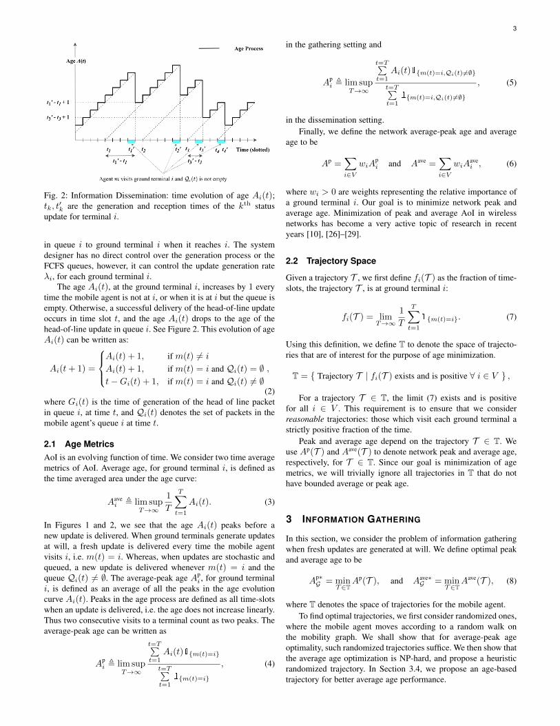
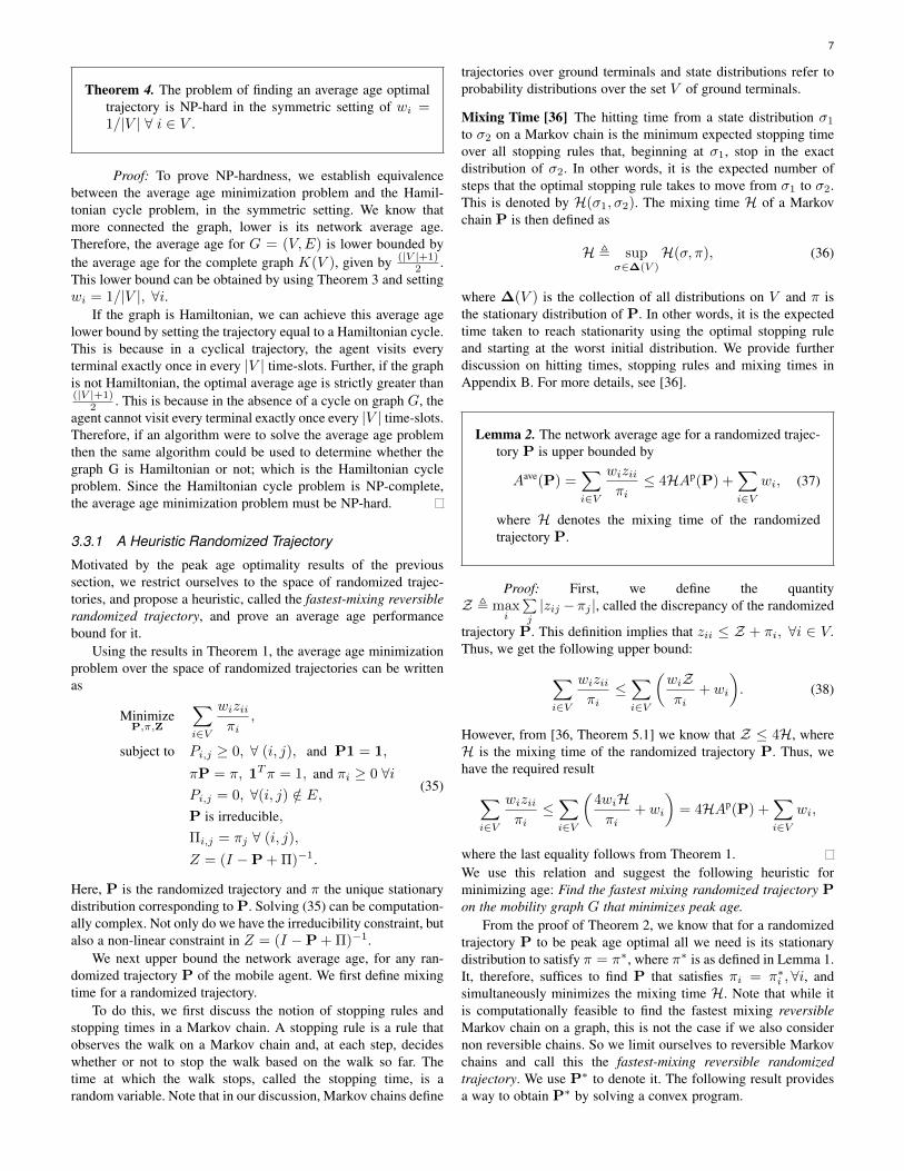
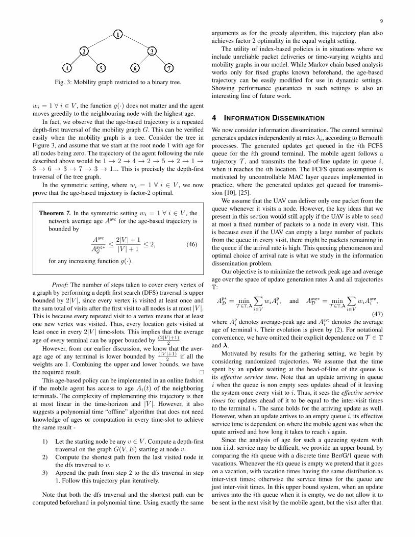
Fig. 3: Mobility graph restricted to a binary tree.

wi = 1 ∀ i ∈ V , the function g(·) does not matter and the agentmoves greedily to the neighbouring node with the highest age.

In fact, we observe that the age-based trajectory is a repeateddepth-first traversal of the mobility graph G. This can be verifiedeasily when the mobility graph is a tree. Consider the tree inFigure 3, and assume that we start at the root node 1 with age forall nodes being zero. The trajectory of the agent following the ruledescribed above would be 1 → 2 → 4 → 2 → 5 → 2 → 1 →3 → 6 → 3 → 7 → 3 → 1... This is precisely the depth-firsttraversal of the tree graph.

In the symmetric setting, where wi = 1 ∀ i ∈ V , we nowprove that the age-based trajectory is factor-2 optimal.

Theorem 7. In the symmetric setting wi = 1 ∀ i ∈ V , thenetwork average age Aave for the age-based trajectory isbounded by

Aave

Aave∗G≤ 2|V |+ 1

|V |+ 1≤ 2, (46)

for any increasing function g(·).

Proof: The number of steps taken to cover every vertex ofa graph by performing a depth first search (DFS) traversal is upperbounded by 2|V |, since every vertex is visited at least once andthe sum total of visits after the first visit to all nodes is at most |V |.This is because every repeated visit to a vertex means that at leastone new vertex was visited. Thus, every location gets visited atleast once in every 2|V | time-slots. This implies that the averageage of every terminal can be upper bounded by (2|V |+1)

2 .However, from our earlier discussion, we know that the aver-

age age of any terminal is lower bounded by (|V |+1)2 if all the

weights are 1. Combining the upper and lower bounds, we havethe required result.

This age-based policy can be implemented in an online fashionif the mobile agent has access to age Ai(t) of the neighboringterminals. The complexity of implementing this trajectory is thenat most linear in the time-horizon and |V |. However, it alsosuggests a polynomial time “offline” algorithm that does not needknowledge of ages or computation in every time-slot to achievethe same result -

1) Let the starting node be any v ∈ V . Compute a depth-firsttraversal on the graph G(V,E) starting at node v.

2) Compute the shortest path from the last visited node inthe dfs traversal to v.

3) Append the path from step 2 to the dfs traversal in step1. Follow this trajectory plan iteratively.

Note that both the dfs traversal and the shortest path can becomputed beforehand in polynomial time. Using exactly the same

arguments as for the greedy algorithm, this trajectory plan alsoachieves factor 2 optimality in the equal weight setting.

The utility of index-based policies is in situations where weinclude unreliable packet deliveries or time-varying weights andmobility graphs in our model. While Markov chain based analysisworks only for fixed graphs known beforehand, the age-basedtrajectory can be easily modified for use in dynamic settings.Showing performance guarantees in such settings is also aninteresting line of future work.

4 INFORMATION DISSEMINATION

We now consider information dissemination. The central terminalgenerates updates independently at rates λi, according to Bernoulliprocesses. The generated updates get queued in the ith FCFSqueue for the ith ground terminal. The mobile agent follows atrajectory T , and transmits the head-of-line update in queue i,when it reaches the ith location. The FCFS queue assumption ismotivated by uncontrollable MAC layer queues implemented inpractice, where the generated updates get queued for transmis-sion [10], [25].

We assume that the UAV can deliver only one packet from thequeue whenever it visits a node. However, the key ideas that wepresent in this section would still apply if the UAV is able to sendat most a fixed number of packets to a node in every visit. Thisis because even if the UAV can empty a large number of packetsfrom the queue in every visit, there might be packets remaining inthe queue if the arrival rate is high. This queuing phenomenon andoptimal choice of arrival rate is what we study in the informationdissemination problem.

Our objective is to minimize the network peak age and averageage over the space of update generation rates λ and all trajectoriesT:

Ap∗D = min

T ∈T,λ

∑i∈V

wiApi , and Aave∗

D = minT ∈T,λ

∑i∈V

wiAavei ,

(47)where Ap

i denotes average-peak age and Aavei denotes the average

age of terminal i. Their evolution is given by (2). For notationalconvenience, we have omitted their explicit dependence on T ∈ Tand λ.

Motivated by results for the gathering setting, we begin byconsidering randomized trajectories. We assume that the timespent by an update waiting at the head-of-line of the queue isits effective service time. Note that an update arriving in queuei when the queue is non empty sees updates ahead of it leavingthe system once every visit to i. Thus, it sees the effective servicetimes for updates ahead of it to be equal to the inter-visit timesto the terminal i. The same holds for the arriving update as well.However, when an update arrives to an empty queue i, its effectiveservice time is dependent on where the mobile agent was when theupate arrived and how long it takes to reach i again.

Since the analysis of age for such a queueing system withnon i.i.d. service may be difficult, we provide an upper bound, bycomparing the ith queue with a discrete time Ber/G/1 queue withvacations. Whenever the ith queue is empty we pretend that it goeson a vacation, with vacation times having the same distribution asinter-visit times; otherwise the service times for the queue arejust inter-visit times. In this upper bound system, when an updatearrives into the ith queue when it is empty, we do not allow it tobe sent in the next visit by the mobile agent, but the visit after that.

10

This ensures i.i.d. service times and vacation times and allows usto analyze the system.

The age process of such an FCFS queue is clearly an upperbound for the age process Ai(t). This is because the total timein the system for packets arriving into a non-empty queue areidentically distributed to the original FCFS queue while packetsarriving into an empty queue in the upper bound system spentextra time waiting. Thus, we upper bound the peak age Ap

i andaverage age Aave

i , by the peak and average age of this Ber/G/1queue with vacations. We first analyze peak and average age of aBer/G/1 queue with i.i.d. vacations and service times.

4.1 Age for Ber/G/1 Queue with VacationsConsider a FCFS Ber/G/1 queue with vacations, where an arrivaloccurs with probability λ, the service times S are generallydistributed with mean E [S] = 1/µ, and the vacation times Vare also distributed the same as S.

We obtain an expression for the average-peak age of a discretetime Ber/G/1 queue with vacations. Further, we derive an upperbound on average age under a negative correlation assumption.

Lemma 3. The average-peak age for a discrete time FCFSBer/G/1 queue with i.i.d. vacations and service is givenby

Ap =1

λ+

1

µ+λE[S2]− ρ

2(1− ρ)+

E[V 2]

2E [V ]− 1

2, (48)

where ρ = λµ , while the average age is upper-bounded by

peak age, namely Aave ≤ Ap.

Proof: The peak age for a FCFS queue is given by

Ap = E [T +X] , (49)

where T denotes the time an update spends in the queue and Xis the inter-arrival time between two updates. Given that vacationtimes are distributed i.i.d according to random variable V , we have

E[T ] =λE[S2]− ρ

2(1− ρ)+

1

µ+

E[V 2]

2E [V ]− 1

2, (50)

where S denotes the service time distribution. Substituting thisand E [X] = 1

λ in (49), we obtain the expression for peak age. Wenow derive the expression for average system time E [T ] seen in(50).

4.1.1 Derivation of System TimeThe proof is a discretized version of the proof for M/G/1 queueswith vacations using residual service times as discussed in [39].

Let us define the residual service time for an update at time t,given by R(t), as the amount of time remaining until the updatecurrently at the head of the queue is complete, excluding thecurrent time-slot. If the queue is empty, R(t) equals zero.

From [39] we know that the expected waiting time in the queuecan be found using the residual service times as follows

E [TQ] =E [R]

1− ρ, (51)

where ρ = λµ , E [S] = 1

µ and E [R] = limT→∞

E[

1T

t=T∑t=0

R(t)

].

As in [39], E [R] can be computed using a graphical argument.

Let service times for the mth packet be Xm, and let the kthvacation time be Vk. Let the total number of packets served beM(T ) and the total number of vacations be L(T ), over the entiretime-horizon T . Then, we have

1

T

t=T∑t=0

R(t) =1

2

M(T )

T

M(T )∑m=1

(X2m −Xm)

M(T )

+1

2

L(T )

T

L(T )∑k=1

(V 2k − Vk)

L(T ). (52)

Using the strong law of large numbers and the fact that M(T )T → λ

and L(T )T → (1−ρ)

E[V ] , we get

E [R] =λ(E

[S2]− E [S])

2+

(1− ρ)(E[V 2]− E [V ])

2E [V ]. (53)

Combining (51), (53), and the fact that total time spent in thesystem by a packet is given by the sum of its waiting time in thequeue and its processing time, we get

E [T ] = E [S + TQ] =1

µ+λE[S2]− ρ

2(1− ρ)+

E[V 2]

2E [V ]− 1

2, (54)

since E [S] = 1µ . We now show the second part of the Lemma,

that the average age is upper bounded by the peak age.

4.1.2 Average AgeConsider a FCFS Ber/G/1 queue with i.i.d. vacations and servicetimes. Let the packet inter-arrival times be X1, X2, ... Let Tn bethe total time spent in the system by the nth packet. Then, theaverage age is given by [6]:

Aave =1

λ+ λE[XnTn], (55)

where 1λ = E[Xn]. To evaluate the term E[XnTn], we observe

that larger inter-arrival times Xn between packets mean lesserwait times in the system Tn for individual packets. This suggestsXn and Tn are negatively correlated and that E [XnTn] ≤E [Xn]E [Tn] . This is a commonly stated observation in AoIliterature [6], [40] but a general proof hasn’t appeared before.In Appendix D we provide a proof of this result for FCFS queueswith no vacations. Proving this for our vacation system becomeschallienging, but we provide simulation results which stronglyindicate that the result holds in both the original system andBer/G/1 queues with i.i.d. vacations and service times. Therefore,we present this result as the assumption below:

Assumption 1. Consider a Ber/G/1 queue with i.i.d. vacationsand service times, where the distribution of a vacation isthe same as that of a service time. Then, packet inter-arrival times Xn are negatively correlated with packetsystem times Tn, i.e.

E [XnTn] ≤ E [Xn]E [Tn] . (56)

If Assumption 1 is true, then we have the required result:

Aave ≤ 1

λ+ λE[Xn]E [Tn] = E [Xn] + E [Tn] = Ap.

11

For the remainder of this work, we assume that Assumption 1holds and the average age Aave is upper bounded by peak age Ap.

4.2 Age Minimization Problem

Using Lemma 3, we now obtain an upper-bound on both networkpeak and average age for a given randomized trajectory P andupdate generation rates λ.

Lemma 4. For a randomized trajectory P and packet gen-eration rates λ, the peak and average age for a groundterminal i is upper-bounded by

AUBi =

1

πi

[1 + zii +

1

ρi+

ziiρi1− ρi

]− ρi

1− ρi− 1,

(57)for all i ∈ V , where π is the unique stationary distributionof P, Z = (I −P + Π)−1, Π is a matrix with all rowsequal to the stationary distribution vector π, and ρi , λi

πi.

Proof: See Appendix E.We propose a policy, i.e. a randomized trajectory P and update

generation rate λ, that minimizes the age upper-bound AUB =∑i∈V wiA

UBi :

Definition Separation Principle Policy

1) Mobile agent follows the randomized trajectory P∗

obtained by solving (39).2) Generate updates for the ground terminal i at rate

λ∗i =π∗i

1 +√z∗ii − π∗i

, (58)

where π∗i =√wi∑

j∈V wjand zii are diagonal elements

of the matrix Z = (I −P∗ + Π∗)−1.

We call it the separation principle policy for two reasons.Firstly, P∗ is the fastest-mixing randomized trajectory, which weproposed for minimizing average age earlier. Secondly, the updategeneration rate for the ground terminal i, depends only on zii andπi, which are functions of the first and second moments of thereturn times to terminal i under trajectory P∗ (see (16) and (17)).We now bound the performance of this separation principle policy.

Theorem 8. The peak and average age of the separationprinciple policy is bounded by

Ap

Ap∗D≤ 4H+ 4

√H+ 2 and

Aave

Aave∗D≤ 8H+ 8

√H+ 4,

where H is the mixing time of the randomized trajectoryP∗.

Proof: We formulate the upper bound age minimizationproblem and use an approach similar to Lemma 2 and Theorem

7. We want to solve the upper bound age minimization problem,which can be stated as:

MinimizeP,ρ

∑i∈V

wiAUBi ,

subject to Pi,j ≥ 0, ∀(i, j),P1 = 1,

Pi,j = 0, ∀(i, j) /∈ E,P is irreducible.

(59)

We first find the optimal packet generation rates given a randomwalk P. Observe that the optimal queue utilization factors ρi canbe solved for given any fixed irreducible random walk P, i.e.

ρ∗i (P) = arg minρi∈[0,1]

AUBi (P, ρi) =

1

1 +√zii − πi

(60)

Note that zii ≥ πi so the equation above is well defined. This isbecause var(Hi) ≥ 0 and the first and second moments of Hi aregiven by (16) and (17). Now, the age under ρ∗i (P) is given by:

minρi∈[0,1]

AUBi (P, ρi) = AUB

i (P, ρ∗i ) =zii − πi + 2

√zii − πi + 2

πi.

(61)Thus, the upper bound age minimization problem reduces to

MinimizeP

∑i∈V

wi

(zii − πi + 2

√zii − πi + 2

πi

),

subject to Pi,j ≥ 0, ∀(i, j),P1 = 1,

Pi,j = 0, ∀(i, j) /∈ E,P is irreducible.

(62)

Now, we can relate the network age upper bound, given arandom walk P, to its mixing time H. We assume optimal packetgeneration rates ρ∗i (P).∑i∈V

wiAUBi (P, ρ∗i (P )) =

∑i∈V

wi

(zii − πi + 2

√zii − πi + 2

πi

),

≤∑i∈V

wi

(Z + 2√Z + 2

πi

),

≤∑i∈V

wi

(4H+ 4

√H+ 2

πi

),

where inequalities follow from the same argument as in the proofof Lemma 2. Setting P = P∗, we obtain∑i∈V

wiAUBi (P∗, ρ∗i (P

∗)) ≤∑i∈V

wi

(4H+ 4

√H+ 2

π∗i

), (63)

where H is the mixing time of P ∗. Note that∑i∈V

wi

π∗iis the

optimal peak age for information gathering, i.e. Ap∗G =

∑i∈V

wi

π∗i.

This gives,

AUB(P∗,ρ∗)

Ap∗G

≤ 4H+ 4√H+ 2. (64)

Due to the presence of queues we have Ap∗G ≤ Ap∗

D . This, (64),and the fact that Ap(P∗,ρ∗) ≤ AUB(P∗,ρ∗), yields the peak agebound on the separation principle policy:

Ap(P∗, λ∗)

Ap∗D

≤ 4H+ 4√H+ 2,

since ρ∗ = λ∗.

12

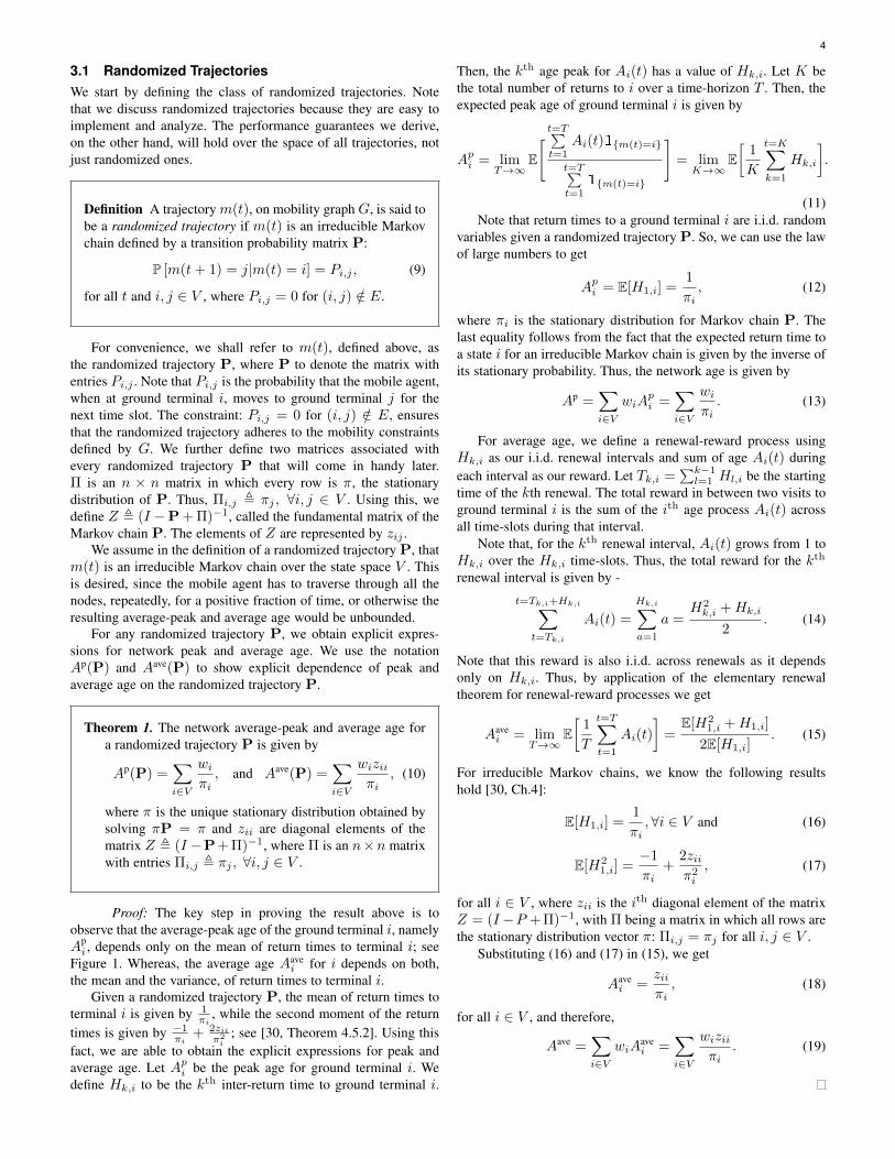
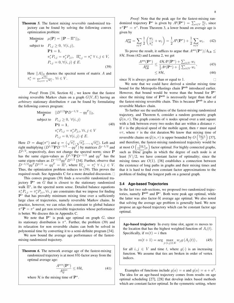
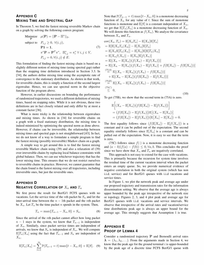
(a) (b) (c)

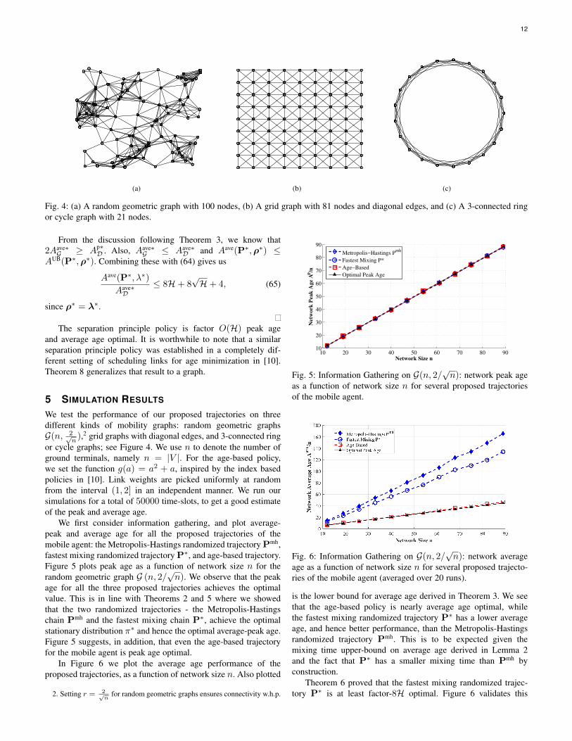
Fig. 4: (a) A random geometric graph with 100 nodes, (b) A grid graph with 81 nodes and diagonal edges, and (c) A 3-connected ringor cycle graph with 21 nodes.

From the discussion following Theorem 3, we know that2Aave∗G ≥ Ap∗

D . Also, Aave∗G ≤ Aave∗

D and Aave(P∗,ρ∗) ≤AUB(P∗,ρ∗). Combining these with (64) gives us

Aave(P∗, λ∗)

Aave∗D

≤ 8H+ 8√H+ 4, (65)

since ρ∗ = λ∗.

The separation principle policy is factor O(H) peak ageand average age optimal. It is worthwhile to note that a similarseparation principle policy was established in a completely dif-ferent setting of scheduling links for age minimization in [10].Theorem 8 generalizes that result to a graph.

5 SIMULATION RESULTS

We test the performance of our proposed trajectories on threedifferent kinds of mobility graphs: random geometric graphsG(n, 2√

n),2 grid graphs with diagonal edges, and 3-connected ring

or cycle graphs; see Figure 4. We use n to denote the number ofground terminals, namely n = |V |. For the age-based policy,we set the function g(a) = a2 + a, inspired by the index basedpolicies in [10]. Link weights are picked uniformly at randomfrom the interval (1, 2] in an independent manner. We run oursimulations for a total of 50000 time-slots, to get a good estimateof the peak and average age.

We first consider information gathering, and plot average-peak and average age for all the proposed trajectories of themobile agent: the Metropolis-Hastings randomized trajectory Pmh,fastest mixing randomized trajectory P∗, and age-based trajectory.Figure 5 plots peak age as a function of network size n for therandom geometric graph G (n, 2/

√n). We observe that the peak

age for all the three proposed trajectories achieves the optimalvalue. This is in line with Theorems 2 and 5 where we showedthat the two randomized trajectories - the Metropolis-Hastingschain Pmh and the fastest mixing chain P∗, achieve the optimalstationary distribution π∗ and hence the optimal average-peak age.Figure 5 suggests, in addition, that even the age-based trajectoryfor the mobile agent is peak age optimal.

In Figure 6 we plot the average age performance of theproposed trajectories, as a function of network size n. Also plotted

2. Setting r = 2√n

for random geometric graphs ensures connectivity w.h.p.

10 20 30 40 50 60 70 80 9010

20

30

40

50

60

70

80

90

Network Size n

Netw

ork

Peak

Age A

p/n

Metropolis−Hastings Pmh

Fastest Mixing P*

Age−Based

Optimal Peak Age

Fig. 5: Information Gathering on G(n, 2/√n): network peak age

as a function of network size n for several proposed trajectoriesof the mobile agent.

Fig. 6: Information Gathering on G(n, 2/√n): network average

age as a function of network size n for several proposed trajecto-ries of the mobile agent (averaged over 20 runs).

is the lower bound for average age derived in Theorem 3. We seethat the age-based policy is nearly average age optimal, whilethe fastest mixing randomized trajectory P∗ has a lower averageage, and hence better performance, than the Metropolis-Hastingsrandomized trajectory Pmh. This is to be expected given themixing time upper-bound on average age derived in Lemma 2and the fact that P∗ has a smaller mixing time than Pmh byconstruction.

Theorem 6 proved that the fastest mixing randomized trajec-tory P∗ is at least factor-8H optimal. Figure 6 validates this

13

20 40 60 80 100 1200

50

100

150

200

250

Network Size n

Netw

ork

Av

era

ge A

ge A

ave /n

Metropolis−Hastings Pmh

Fastest Mixing P*

Age−Based

Lower Bound

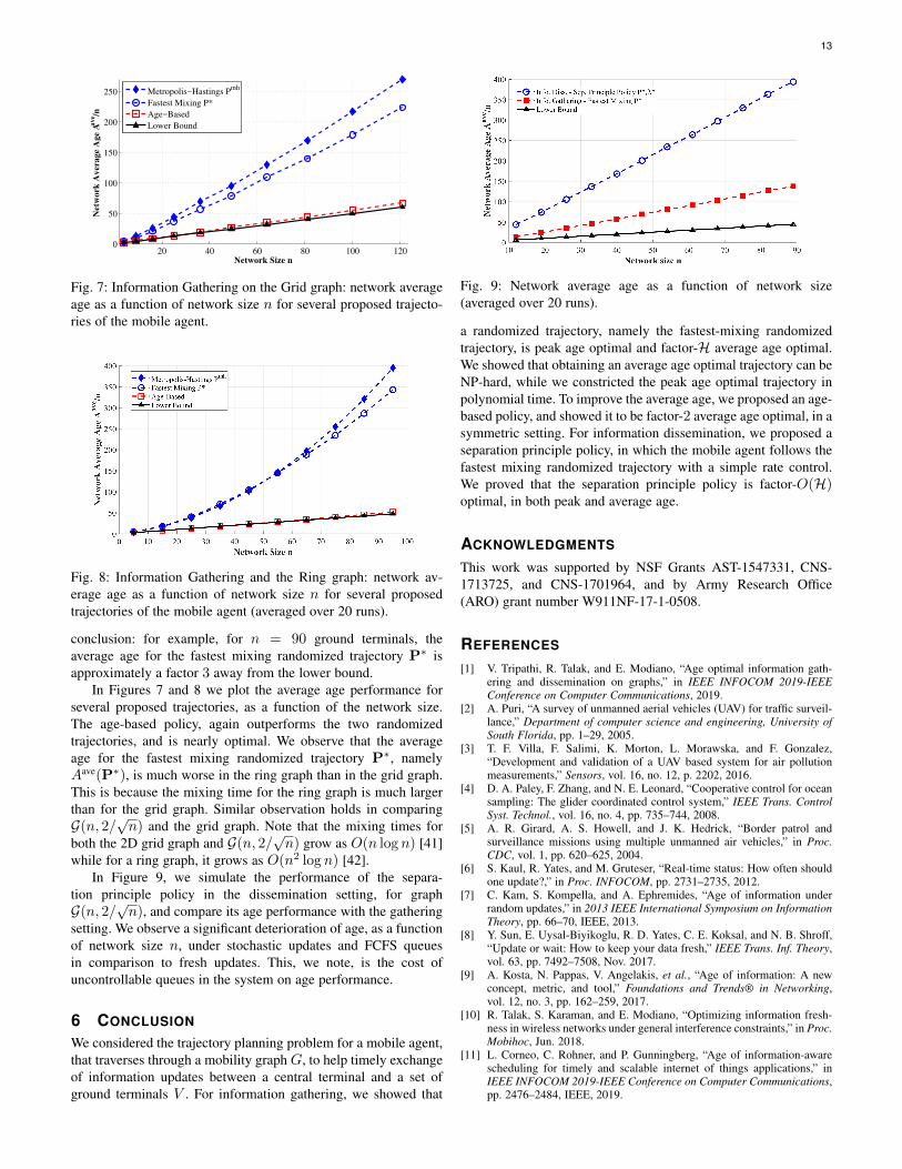
Fig. 7: Information Gathering on the Grid graph: network averageage as a function of network size n for several proposed trajecto-ries of the mobile agent.

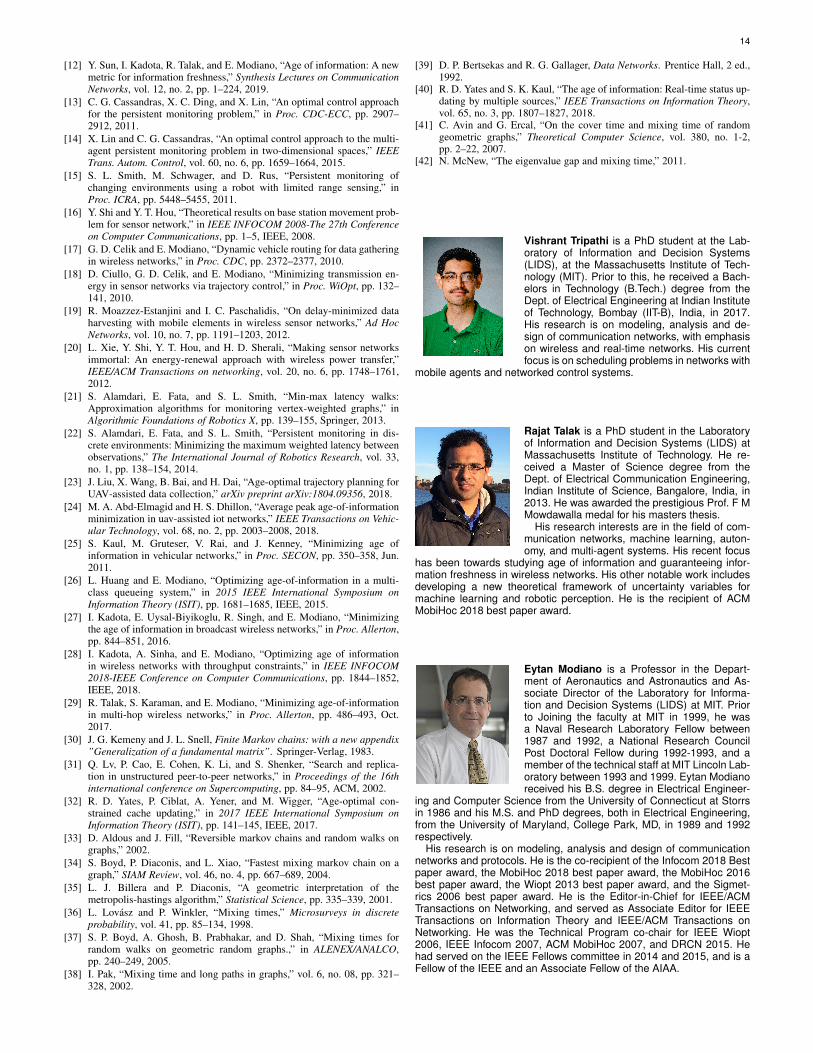
Fig. 8: Information Gathering and the Ring graph: network av-erage age as a function of network size n for several proposedtrajectories of the mobile agent (averaged over 20 runs).

conclusion: for example, for n = 90 ground terminals, theaverage age for the fastest mixing randomized trajectory P∗ isapproximately a factor 3 away from the lower bound.

In Figures 7 and 8 we plot the average age performance forseveral proposed trajectories, as a function of the network size.The age-based policy, again outperforms the two randomizedtrajectories, and is nearly optimal. We observe that the averageage for the fastest mixing randomized trajectory P∗, namelyAave(P∗), is much worse in the ring graph than in the grid graph.This is because the mixing time for the ring graph is much largerthan for the grid graph. Similar observation holds in comparingG(n, 2/

√n) and the grid graph. Note that the mixing times for

both the 2D grid graph and G(n, 2/√n) grow as O(n log n) [41]

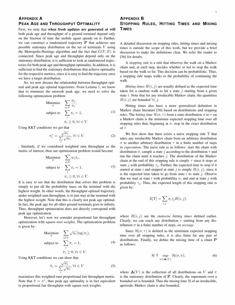
while for a ring graph, it grows as O(n2 log n) [42].In Figure 9, we simulate the performance of the separa-

tion principle policy in the dissemination setting, for graphG(n, 2/

√n), and compare its age performance with the gathering

setting. We observe a significant deterioration of age, as a functionof network size n, under stochastic updates and FCFS queuesin comparison to fresh updates. This, we note, is the cost ofuncontrollable queues in the system on age performance.

6 CONCLUSION

We considered the trajectory planning problem for a mobile agent,that traverses through a mobility graph G, to help timely exchangeof information updates between a central terminal and a set ofground terminals V . For information gathering, we showed that

Fig. 9: Network average age as a function of network size(averaged over 20 runs).

a randomized trajectory, namely the fastest-mixing randomizedtrajectory, is peak age optimal and factor-H average age optimal.We showed that obtaining an average age optimal trajectory can beNP-hard, while we constricted the peak age optimal trajectory inpolynomial time. To improve the average age, we proposed an age-based policy, and showed it to be factor-2 average age optimal, in asymmetric setting. For information dissemination, we proposed aseparation principle policy, in which the mobile agent follows thefastest mixing randomized trajectory with a simple rate control.We proved that the separation principle policy is factor-O(H)optimal, in both peak and average age.

ACKNOWLEDGMENTS

This work was supported by NSF Grants AST-1547331, CNS-1713725, and CNS-1701964, and by Army Research Office(ARO) grant number W911NF-17-1-0508.

REFERENCES

[1] V. Tripathi, R. Talak, and E. Modiano, “Age optimal information gath-ering and dissemination on graphs,” in IEEE INFOCOM 2019-IEEEConference on Computer Communications, 2019.

[2] A. Puri, “A survey of unmanned aerial vehicles (UAV) for traffic surveil-lance,” Department of computer science and engineering, University ofSouth Florida, pp. 1–29, 2005.

[3] T. F. Villa, F. Salimi, K. Morton, L. Morawska, and F. Gonzalez,“Development and validation of a UAV based system for air pollutionmeasurements,” Sensors, vol. 16, no. 12, p. 2202, 2016.

[4] D. A. Paley, F. Zhang, and N. E. Leonard, “Cooperative control for oceansampling: The glider coordinated control system,” IEEE Trans. ControlSyst. Technol., vol. 16, no. 4, pp. 735–744, 2008.

[5] A. R. Girard, A. S. Howell, and J. K. Hedrick, “Border patrol andsurveillance missions using multiple unmanned air vehicles,” in Proc.CDC, vol. 1, pp. 620–625, 2004.

[6] S. Kaul, R. Yates, and M. Gruteser, “Real-time status: How often shouldone update?,” in Proc. INFOCOM, pp. 2731–2735, 2012.

[7] C. Kam, S. Kompella, and A. Ephremides, “Age of information underrandom updates,” in 2013 IEEE International Symposium on InformationTheory, pp. 66–70, IEEE, 2013.

[8] Y. Sun, E. Uysal-Biyikoglu, R. D. Yates, C. E. Koksal, and N. B. Shroff,“Update or wait: How to keep your data fresh,” IEEE Trans. Inf. Theory,vol. 63, pp. 7492–7508, Nov. 2017.

[9] A. Kosta, N. Pappas, V. Angelakis, et al., “Age of information: A newconcept, metric, and tool,” Foundations and Trends® in Networking,vol. 12, no. 3, pp. 162–259, 2017.

[10] R. Talak, S. Karaman, and E. Modiano, “Optimizing information fresh-ness in wireless networks under general interference constraints,” in Proc.Mobihoc, Jun. 2018.

[11] L. Corneo, C. Rohner, and P. Gunningberg, “Age of information-awarescheduling for timely and scalable internet of things applications,” inIEEE INFOCOM 2019-IEEE Conference on Computer Communications,pp. 2476–2484, IEEE, 2019.

14

[12] Y. Sun, I. Kadota, R. Talak, and E. Modiano, “Age of information: A newmetric for information freshness,” Synthesis Lectures on CommunicationNetworks, vol. 12, no. 2, pp. 1–224, 2019.

[13] C. G. Cassandras, X. C. Ding, and X. Lin, “An optimal control approachfor the persistent monitoring problem,” in Proc. CDC-ECC, pp. 2907–2912, 2011.

[14] X. Lin and C. G. Cassandras, “An optimal control approach to the multi-agent persistent monitoring problem in two-dimensional spaces,” IEEETrans. Autom. Control, vol. 60, no. 6, pp. 1659–1664, 2015.

[15] S. L. Smith, M. Schwager, and D. Rus, “Persistent monitoring ofchanging environments using a robot with limited range sensing,” inProc. ICRA, pp. 5448–5455, 2011.

[16] Y. Shi and Y. T. Hou, “Theoretical results on base station movement prob-lem for sensor network,” in IEEE INFOCOM 2008-The 27th Conferenceon Computer Communications, pp. 1–5, IEEE, 2008.

[17] G. D. Celik and E. Modiano, “Dynamic vehicle routing for data gatheringin wireless networks,” in Proc. CDC, pp. 2372–2377, 2010.

[18] D. Ciullo, G. D. Celik, and E. Modiano, “Minimizing transmission en-ergy in sensor networks via trajectory control,” in Proc. WiOpt, pp. 132–141, 2010.

[19] R. Moazzez-Estanjini and I. C. Paschalidis, “On delay-minimized dataharvesting with mobile elements in wireless sensor networks,” Ad HocNetworks, vol. 10, no. 7, pp. 1191–1203, 2012.

[20] L. Xie, Y. Shi, Y. T. Hou, and H. D. Sherali, “Making sensor networksimmortal: An energy-renewal approach with wireless power transfer,”IEEE/ACM Transactions on networking, vol. 20, no. 6, pp. 1748–1761,2012.

[21] S. Alamdari, E. Fata, and S. L. Smith, “Min-max latency walks:Approximation algorithms for monitoring vertex-weighted graphs,” inAlgorithmic Foundations of Robotics X, pp. 139–155, Springer, 2013.

[22] S. Alamdari, E. Fata, and S. L. Smith, “Persistent monitoring in dis-crete environments: Minimizing the maximum weighted latency betweenobservations,” The International Journal of Robotics Research, vol. 33,no. 1, pp. 138–154, 2014.

[23] J. Liu, X. Wang, B. Bai, and H. Dai, “Age-optimal trajectory planning forUAV-assisted data collection,” arXiv preprint arXiv:1804.09356, 2018.

[24] M. A. Abd-Elmagid and H. S. Dhillon, “Average peak age-of-informationminimization in uav-assisted iot networks,” IEEE Transactions on Vehic-ular Technology, vol. 68, no. 2, pp. 2003–2008, 2018.

[25] S. Kaul, M. Gruteser, V. Rai, and J. Kenney, “Minimizing age ofinformation in vehicular networks,” in Proc. SECON, pp. 350–358, Jun.2011.

[26] L. Huang and E. Modiano, “Optimizing age-of-information in a multi-class queueing system,” in 2015 IEEE International Symposium onInformation Theory (ISIT), pp. 1681–1685, IEEE, 2015.

[27] I. Kadota, E. Uysal-Biyikoglu, R. Singh, and E. Modiano, “Minimizingthe age of information in broadcast wireless networks,” in Proc. Allerton,pp. 844–851, 2016.

[28] I. Kadota, A. Sinha, and E. Modiano, “Optimizing age of informationin wireless networks with throughput constraints,” in IEEE INFOCOM2018-IEEE Conference on Computer Communications, pp. 1844–1852,IEEE, 2018.

[29] R. Talak, S. Karaman, and E. Modiano, “Minimizing age-of-informationin multi-hop wireless networks,” in Proc. Allerton, pp. 486–493, Oct.2017.

[30] J. G. Kemeny and J. L. Snell, Finite Markov chains: with a new appendix”Generalization of a fundamental matrix”. Springer-Verlag, 1983.

[31] Q. Lv, P. Cao, E. Cohen, K. Li, and S. Shenker, “Search and replica-tion in unstructured peer-to-peer networks,” in Proceedings of the 16thinternational conference on Supercomputing, pp. 84–95, ACM, 2002.

[32] R. D. Yates, P. Ciblat, A. Yener, and M. Wigger, “Age-optimal con-strained cache updating,” in 2017 IEEE International Symposium onInformation Theory (ISIT), pp. 141–145, IEEE, 2017.

[33] D. Aldous and J. Fill, “Reversible markov chains and random walks ongraphs,” 2002.

[34] S. Boyd, P. Diaconis, and L. Xiao, “Fastest mixing markov chain on agraph,” SIAM Review, vol. 46, no. 4, pp. 667–689, 2004.

[35] L. J. Billera and P. Diaconis, “A geometric interpretation of themetropolis-hastings algorithm,” Statistical Science, pp. 335–339, 2001.

[36] L. Lovasz and P. Winkler, “Mixing times,” Microsurveys in discreteprobability, vol. 41, pp. 85–134, 1998.

[37] S. P. Boyd, A. Ghosh, B. Prabhakar, and D. Shah, “Mixing times forrandom walks on geometric random graphs.,” in ALENEX/ANALCO,pp. 240–249, 2005.

[38] I. Pak, “Mixing time and long paths in graphs,” vol. 6, no. 08, pp. 321–328, 2002.

[39] D. P. Bertsekas and R. G. Gallager, Data Networks. Prentice Hall, 2 ed.,1992.

[40] R. D. Yates and S. K. Kaul, “The age of information: Real-time status up-dating by multiple sources,” IEEE Transactions on Information Theory,vol. 65, no. 3, pp. 1807–1827, 2018.

[41] C. Avin and G. Ercal, “On the cover time and mixing time of randomgeometric graphs,” Theoretical Computer Science, vol. 380, no. 1-2,pp. 2–22, 2007.

[42] N. McNew, “The eigenvalue gap and mixing time,” 2011.

Vishrant Tripathi is a PhD student at the Lab-oratory of Information and Decision Systems(LIDS), at the Massachusetts Institute of Tech-nology (MIT). Prior to this, he received a Bach-elors in Technology (B.Tech.) degree from theDept. of Electrical Engineering at Indian Instituteof Technology, Bombay (IIT-B), India, in 2017.His research is on modeling, analysis and de-sign of communication networks, with emphasison wireless and real-time networks. His currentfocus is on scheduling problems in networks with

mobile agents and networked control systems.

Rajat Talak is a PhD student in the Laboratoryof Information and Decision Systems (LIDS) atMassachusetts Institute of Technology. He re-ceived a Master of Science degree from theDept. of Electrical Communication Engineering,Indian Institute of Science, Bangalore, India, in2013. He was awarded the prestigious Prof. F MMowdawalla medal for his masters thesis.

His research interests are in the field of com-munication networks, machine learning, auton-omy, and multi-agent systems. His recent focus

has been towards studying age of information and guaranteeing infor-mation freshness in wireless networks. His other notable work includesdeveloping a new theoretical framework of uncertainty variables formachine learning and robotic perception. He is the recipient of ACMMobiHoc 2018 best paper award.

Eytan Modiano is a Professor in the Depart-ment of Aeronautics and Astronautics and As-sociate Director of the Laboratory for Informa-tion and Decision Systems (LIDS) at MIT. Priorto Joining the faculty at MIT in 1999, he wasa Naval Research Laboratory Fellow between1987 and 1992, a National Research CouncilPost Doctoral Fellow during 1992-1993, and amember of the technical staff at MIT Lincoln Lab-oratory between 1993 and 1999. Eytan Modianoreceived his B.S. degree in Electrical Engineer-

ing and Computer Science from the University of Connecticut at Storrsin 1986 and his M.S. and PhD degrees, both in Electrical Engineering,from the University of Maryland, College Park, MD, in 1989 and 1992respectively.

His research is on modeling, analysis and design of communicationnetworks and protocols. He is the co-recipient of the Infocom 2018 Bestpaper award, the MobiHoc 2018 best paper award, the MobiHoc 2016best paper award, the Wiopt 2013 best paper award, and the Sigmet-rics 2006 best paper award. He is the Editor-in-Chief for IEEE/ACMTransactions on Networking, and served as Associate Editor for IEEETransactions on Information Theory and IEEE/ACM Transactions onNetworking. He was the Technical Program co-chair for IEEE Wiopt2006, IEEE Infocom 2007, ACM MobiHoc 2007, and DRCN 2015. Hehad served on the IEEE Fellows committee in 2014 and 2015, and is aFellow of the IEEE and an Associate Fellow of the AIAA.

1

APPENDIX APEAK AGE AND THROUGHPUT OPTIMALITY

First, we note that when fresh updates are generated at willboth peak age and throughput of a ground terminal depend onlyon the fraction of time the mobile agent spends on it. Further,we can construct a randomized trajectory P that achieves anypossible stationary distribution on the set of terminals V usingthe Metropolis-Hastings algorithm and the fact that G(V,E) isconnected. Since peak age and throughput depend only on thestationary distribution, it is sufficient to look at randomized trajec-tories for both peak age and throughput optimality. In addition, it issufficient to find the stationary distributions that achieve optimalityfor the respective metrics, since it is easy to find the trajectory oncewe have a target distribution.

So, we now discuss the relationship between throughput opti-mal and peak age optimal trajectories. From Lemma 1, we knowthat to minimize the network peak age, we need to solve thefollowing optimization problem

Minimizeπ

∑i∈V

wiπi,

subject to∑i

πi = 1,

πi ≥ 0,∀i ∈ V.

(1)

Using KKT conditions we get that

π∗i =

√wi∑

i

√wi,∀i ∈ V. (2)

. Similarly, if we considered weighted sum throughput as themetric of interest, then our optimization problem would become

Maximizeπ

∑i∈V

wiπi,

subject to∑i

πi = 1,

πi ≥ 0,∀i ∈ V.

(3)

It is easy to see that the distribution that solves this problem issimply to put all the probability mass on the terminal with thehighest weight. In other words, the throughput optimal trajectory,under weighted-sum throughput, is to just stay at the terminal withthe highest weight. Note that this is clearly not peak age optimal.In fact, the peak age for all other ground terminals goes to infinity.Thus, throughput optimization does not directly correspond withpeak age optimization.

However, let’s now we consider proportional fair throughputoptimization with square-root weights. The optimization problemis given by:

Maximizeπ

∑i∈V

√wi log(πi),

subject to∑i

πi = 1,

πi ≥ 0,∀i ∈ V.

(4)

Using KKT conditions we can show that

πi =

√wi∑

i

√wi,∀i ∈ V (5)

maximizes this weighted-sum proportional fair throughput metric.Note that π = π∗, thus peak age optimality is in fact equivalentto proportional fair throughput with square root weights.

APPENDIX BSTOPPING RULES, HITTING TIMES AND MIXINGTIMES

A detailed discussion on stopping rules, hitting times and mixingtimes is outside the scope of this work, but we provide a briefdiscussion to make the definitions clear. We refer the reader to[36] for details.

A stopping rule is a rule that observes the walk on a Markovchain and, at each step, decides whether or not to stop the walkbased on the walk so far. This decision can be probabilistic. Thus,a stopping rule maps walks to the probability of continuing thewalk.

Hitting times H(i, j) are usually defined as the expected timetaken for a random walk to hit a state j starting from a givenstate i. Note that for any irreducible Markov chain, the quantitiesH(i, j) are bounded ∀i, j.

Hitting times also have a more generalized definition inMarkov chain literature [36] based on distributions and stoppingrules. The hitting time H(σ, τ) from a state distribution σ to τ ona Markov chain is the minimum expected stopping time over allstopping rules that, beginning at σ, stop in the exact distributionof τ .

We first show that there exists a naive stopping rule T thattakes any irreducible Markov chain from an arbitrary distributionσ to another arbitrary distribution τ in a finite number of stepsin expectation. The naive rule is as follows: start the chain withdistribution σ, sample a state j according to the distribution τ andrun the chain until it reaches j. The distribution of the Markovchain at the end of this stopping rule is simply τ since it stops atstate j with probability τj . Further, the expected time to stop if itstarted at state i and stopped at state j is simply H(i, j), since itis the expected time taken to go from state i to state j. Observethat we start at state i with probability σi and end at state j withprobabiltiy τj . Thus, the expected length of this stopping rule isgiven by:

E[T] =∑i,j

σiτjH(i, j).

where H(i, j) are the statewise hitting times defined earlier.Clearly, we can reach any distribution τ starting from any dis-tribution σ in a finite number of steps, on average.

Since H(σ, τ) is defined as the minimum expected stoppingtime over all stopping rules, it is also finite for any pair ofdistributions. Finally, we define the mixing time of a chain Pas follows:

H , supσ∈∆(V )

H(σ, π), (6)

where ∆(V ) is the collection of all distributions on V and πis the stationary distribution of P. Clearly, the supremum over abounded set is bounded. Thus the mixing timeH of an irreducible,aperiodic Markov chain is also bounded.

2

APPENDIX CMIXING TIME AND SPECTRAL GAP

In Theorem 5, we find the fastest mixing reversible Markov chainon a graph by solving the following convex program:

MinimizeP

µ(P) = ||P−Π∗||2,

subject to Pi,j ≥ 0, ∀(i, j),P1 = 1,

π∗P = PTπ∗, Π∗i,j = π∗i ∀ i, j ∈ V,Pi,j = 0,∀(i, j) /∈ E.

(7)

This formulation of finding the fastest mixing chain is based on aslightly different notion of mixing time (using spectral gap) ratherthan the stopping time definition introduced in Section 3.3. In[34], the authors define mixing time using the asymptotic rate ofconvergence to the stationary distribution. As shown in that work,for reversible chains, this is simply a function of the second largesteigenvalue. Hence, we can use spectral norm in the objectivefunction of the program above.

However, in earlier discussions on bounding the performanceof randomized trajectories, we used a different definition of mixingtimes, based on stopping rules. While it is not obvious, these twodefinitions are in fact closely related and only differ by at most aconstant factor [36].

What is more tricky is the relationship between eigenvaluesand mixing times. As shown in [34] for reversible chains ona graph with a fixed stationary distribution, the mixing time isindeed minimized by optimizing the spectral norm as done above.However, if chains can be irreversible, the relationship betweenmixing times and spectral gaps is not straightforward [43]. In fact,we do not know of a way to formulate a simple program to findthe fastest mixing (possibly irreversible) Markov chain on a graph.

A simple way to get around this is to find the fastest mixingreversible Markov chain using (39) and also a relaxation of (39)over irreversible chains by replacing local balance constraints withglobal balance. Then, we can use whichever trajectory that has thelower mixing time. This ensures that we do not restrict ourselvesto reversible chains in practice. However, we cannot guarantee thatthe chain found is the fastest mixing over all trajectories, includingirreversible ones, but just the reversible ones.

APPENDIX DNEGATIVE CORRELATION OF Xn AND Tn

We first prove the result for Ber/G/1 FCFS queues with novacations. Let the service time of the nth packet be Sn and let theinter-arrival time between the n − 1th packet and the nth packetbe Xn. Let Tn be the time packet n spends in the system. Then,

Tn = max{Tn−1 −Xn, 0}+ Sn. (8)

Since the arrival of the nth packet cannot affect how long packetn − 1 stays in the system, we know that Tn−1 is independentof Xn. Similarly, since packet service times are independent ofarrivals, we know that Sn is independent of Xn. We will computeE[Tn|Xn] using the fact that Tn−1 and Sn are independent ofXn.

E[Tn|Xn] =∞∑t=1

P(Tn−1 = t) max{t−Xn, 0}+ E[S]. (9)

Note that P(Tn−1 = t) max{t−Xn, 0} is a monotone decreasingfunction of Xn for any value of t. Since the sum of monotonefunctions is monotone and E[S] is a constant independent of Xn,we get that E[Tn|Xn] is a monotone decreasing function of Xn.We will denote this function as f(Xn). We analyze the covariancebetween Xn and Tn.

cov(Xn, Tn) = E[XnTn]− E[Xn]E[Tn]

= E[E[XnTn|Xn]]− E[Xn]E[Tn]

= E[XnE[Tn|Xn]]− E[Xn]E[E[Tn|Xn]]

= E[Xnf(Xn)]− E[Xn]E[f(Xn)]

= E[(Xn − E[Xn])(f(Xn)− E[f(Xn)])]

= E[(Xn − E[Xn])(f(Xn)− E[f(Xn)] + f(E[Xn])− f(E[Xn]))]

(75A)= E[(Xn − E[Xn])(f(Xn)− f(E[Xn]))]

+ E[(Xn − E[Xn])(f(E[Xn])− E[f(Xn)])]

(75B)= E[(Xn − E[Xn])(f(Xn)− f(E[Xn]))]

(75C)

≤ 0,(10)

To get (75B), we show that the second term in (75A) is zero.

E[(Xn − E[Xn])

(f(E[Xn])− E[f(Xn)]

)]=(f(E[Xn])− E[f(Xn)]

)E[(Xn − E[Xn])

]=(f(E[Xn])− E[f(Xn)]

)(E[Xn]− E[Xn]

)= 0.

The first equality follows since (f(E[Xn]) − E[f(Xn)]) is aconstant and it can be pulled out of the expectation. The secondequality similarly follows since E[Xn] is a constant and can bepulled out of the expectation. Now, it is easy to see that the termis zero.

(75C) follows since f(·) is a monotone decreasing functionand (a − b)(f(a) − f(b)) ≤ 0,∀a, b. This concludes the proofsince we have show that Xn and Tn are negatively correlated.

This approach is not easy to extend for the case with vacations.This is primarily because the recursion for system time involvesthe residual time of the current vacation interval when the packetenters an empty queue. So, we provide numerical evidence ofnegative correlation in both the original system (which has noni.i.d. service) and for Ber/G/1 queues with i.i.d vacations andservice times.

In Figure 1, we plot the network peak and average age underour proposed trajectory and transmission rates for the informationdissemination setting. We observe that the average age is alwaysupper bounded by the peak age irrespective of the network sizeor topology. Figures 2, 3, and 4 plot peak and average age forBer/G/1 queues with i.i.d. vacations and service intervals. Weobserve that irrespective of the arrival rates and vacation/servicetime distributions peak age is always an upper bound for theaverage age. This strongly suggests that Assumption 1 is true.

APPENDIX EPROOF OF LEMMA 4Consider a randomized trajectory P and Bernoulli arrival ratesλ = (λ1, λ2, . . .). From the arguments made in Section 4, weknow that the peak age for the ground terminal i is upper-boundedby the peak age of a discrete time FCFS Ber/G/1 queue with

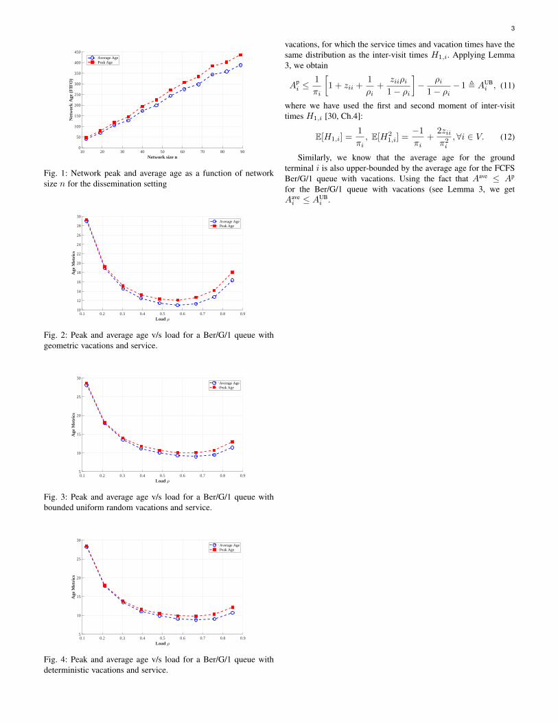
3

10 20 30 40 50 60 70 80 90Network size n

0

50

100

150

200

250

300

350

400

450

Net

wor

k A

ge (

FIF

O)

Average AgePeak Age

Fig. 1: Network peak and average age as a function of networksize n for the dissemination setting

0.1 0.2 0.3 0.4 0.5 0.6 0.7 0.8 0.9Load

10

12

14

16

18

20

22

24

26

28

30

Age

Met

rics

Average AgePeak Age

Fig. 2: Peak and average age v/s load for a Ber/G/1 queue withgeometric vacations and service.

0.1 0.2 0.3 0.4 0.5 0.6 0.7 0.8 0.9Load

5

10

15

20

25

30

Age

Met

rics

Average AgePeak Age

Fig. 3: Peak and average age v/s load for a Ber/G/1 queue withbounded uniform random vacations and service.

0.1 0.2 0.3 0.4 0.5 0.6 0.7 0.8 0.9Load

5

10

15

20

25

30

Age

Met

rics

Average AgePeak Age

Fig. 4: Peak and average age v/s load for a Ber/G/1 queue withdeterministic vacations and service.

vacations, for which the service times and vacation times have thesame distribution as the inter-visit times H1,i. Applying Lemma3, we obtain

Api ≤

1

πi

[1 + zii +

1

ρi+

ziiρi1− ρi

]− ρi

1− ρi− 1 , AUB

i , (11)

where we have used the first and second moment of inter-visittimes H1,i [30, Ch.4]:

E[H1,i] =1

πi, E[H2

1,i] =−1

πi+

2ziiπ2i

,∀i ∈ V. (12)

Similarly, we know that the average age for the groundterminal i is also upper-bounded by the average age for the FCFSBer/G/1 queue with vacations. Using the fact that Aave ≤ Ap

for the Ber/G/1 queue with vacations (see Lemma 3, we getAavei ≤ AUB

i .