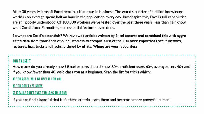
After 30 years, Microsoft Excel remains ubiquitous in business. The world’s quarter of a billion knowledge workers on average spend half an hour in the application every day. But despite this, Excel’s full capabilities are still poorly understood. Of 100,000 workers we've tested over the past three years, less than half know what Conditional Formatting - an essential feature - even does.

So what are Excel’s essentials? We reviewed articles written by Excel experts and combined this with aggre-gated data from thousands of our customers to compile a list of the 100 most important Excel functions, features, tips, tricks and hacks, ordered by utility. Where are your favourites?

How to use it

How many do you already know? Excel experts should know 80+, proficient users 60+, average users 40+ and if you know fewer than 40, we’d class you as a beginner. Scan the list for tricks which:

a) you agree will be useful for you

b) you don’t yet know

c) ideally don’t take too long to learn

If you can find a handful that fulfil these criteria, learn them and become a more powerful human!

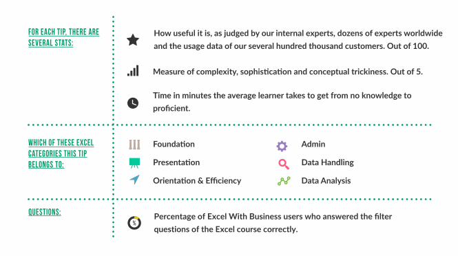
For each tip, there are several stats:

Percentage of Excel With Business users who answered the filter questions of the Excel course correctly.

Foundation

Presentation

Orientation & Efficiency

Admin

Data Handling

Data Analysis

Measure of complexity, sophistication and conceptual trickiness. Out of 5.

How useful it is, as judged by our internal experts, dozens of experts worldwide and the usage data of our several hundred thousand customers. Out of 100.

Which of these Excel categories this tip belongs to:

Time in minutes the average learner takes to get from no knowledge to proficient.

Questions:

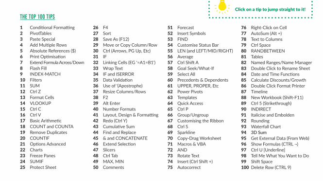
1 Conditional Formatting2 PivotTables3 Paste Special4 Add Multiple Rows5 Absolute References ($)6 Print Optimisation7 Extend Formula Across/Down8 Flash Fill9 INDEX-MATCH10 Filters11 SUM12 Ctrl Z13 Format Cells14 VLOOKUP15 Ctrl C16 Ctrl V17 Basic Arithmetic18 COUNT and COUNTA19 Remove Duplicates20 COUNTIF21 Options Advanced22 Charts23 Freeze Panes24 SUMIF25 Protect Sheet

26 F427 Sort28 Save As (F12)29 Move or Copy Column/Row30 Ctrl (Arrows, PG Up, Etc)31 IF32 Linking Cells (EG '=A1=B1')33 Wrap Text34 IF and ISERROR35 Data Validation36 Use of '(Apostrophe)37 Resize Columns/Rows38 F239 Alt Enter40 Number Formats41 Layout, Design & Formatting42 Redo (Ctrl Y)43 Cumulative Sum44 Find and Replace45 & and CONCATENATE46 Extend Selection47 Slicers48 Ctrl Tab49 MAX, MIN50 Comments

51 Forecast52 Insert Symbols53 FIND54 Customise Status Bar55 LEN (and LEFT/MID/RIGHT)56 Average57 Ctrl Shift A58 Goal Seek/What-If59 Select All60 Precedents & Dependents61 UPPER, PROPER, Etc62 Power Pivots63 Templates64 Quick Access65 Ctrl P66 Group/Ungroup67 Customising the Ribbon68 Ctrl S69 Sparkline70 Copy-Drag Worksheet71 Macros & VBA72 AND73 Rotate Text74 Insert (Ctrl Shift +)75 Autocorrect

76 Right-Click on Cell77 AutoSum (Alt =)78 Text to Columns79 Ctrl Space80 RANDBETWEEN81 Tables82 Named Ranges/Name Manager83 Double Click to Rename Sheet84 Date and Time Functions85 Calculate Discounts/Growth86 Double Click Format Printer87 Timeline88 New Workbook (Shift-F11)89 Ctrl 5 (Strikethrough)90 INDIRECT91 Italicise and Embolden92 Rounding93 Waterfall Chart94 3D Sum95 Get External Data (From Web)96 Show Formulas (CTRL ¬)97 Ctrl U [Underline]98 Tell Me What You Want to Do99 Shift Space100 Delete Row (CTRL 9)

The top 100 tipsClick on a tip to jump straight to it!

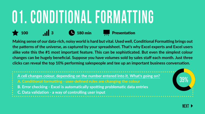
Making sense of our data-rich, noisy world is hard but vital. Used well, Conditional Formatting brings out the patterns of the universe, as captured by your spreadsheet. That's why Excel experts and Excel users alike vote this the #1 most important feature. This can be sophisticated. But even the simplest colour changes can be hugely beneficial. Suppose you have volumes sold by sales staff each month. Just three clicks can reveal the top 10% performing salespeople and tee up an important business conversation.

A cell changes colour, depending on the number entered into it. What's going on?A. Conditional formatting - user-defined rules are changing the colourB. Error checking - Excel is automatically spotting problematic data entriesC. Data validation - a way of controlling user input

01. Conditional Formatting100 3 180 min Presentation

Next

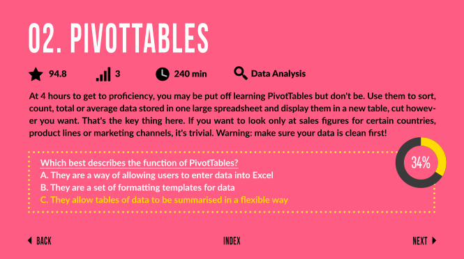
At 4 hours to get to proficiency, you may be put off learning PivotTables but don't be. Use them to sort, count, total or average data stored in one large spreadsheet and display them in a new table, cut howev-er you want. That's the key thing here. If you want to look only at sales figures for certain countries, product lines or marketing channels, it's trivial. Warning: make sure your data is clean first!

Which best describes the function of PivotTables?A. They are a way of allowing users to enter data into ExcelB. They are a set of formatting templates for dataC. They allow tables of data to be summarised in a flexible way

02. PivotTables94.8 3 240 min Data Analysis

Back NextIndex

Back NextIndex

Grabbing (ie Copying) some data from one cell and pasting it into another cell is one of the most common activities in Excel. But there's a lot you might copy (formatting, value, formula, comments, etc) and sometimes you won't want to copy all of it. The most common example of this is where you want to lose the formatting - the place this data is going is your own spreadsheet with your own styling. It's annoying and ugly to plonk in formatting from elsewhere. So just copy the values and all you'll get is the text, number, whatever the value is. The shortcut after copying the cell (Ctrl C) is Alt E S V - easier to do than it sounds.

The other big one is Transpose. This flips rows and columns around in seconds. Shortcut Alt E S E.

03. Paste Special87.9 1 10 min Orientation & Efficiency

Back NextIndex

Probably one of the most frequently carried out activities in spreadsheeting. Ctrl Shift + is the shortcut, but actually it takes longer than just right-clicking on the row numbers on the left of the Excel display. So Right Click is our recommendation. And if you want to add more than one, select as many rows or columns as you'd like to add and then Right Click and add.

04. Add Multiple Rows87.5 0 10 min Orientation & Efficiency

Back NextIndex

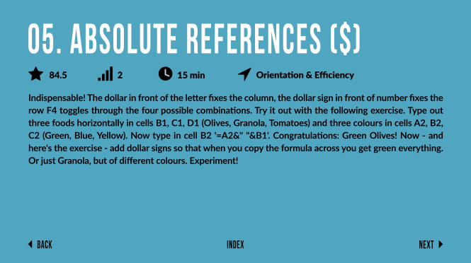
Indispensable! The dollar in front of the letter fixes the column, the dollar sign in front of number fixes the row F4 toggles through the four possible combinations. Try it out with the following exercise. Type out three foods horizontally in cells B1, C1, D1 (Olives, Granola, Tomatoes) and three colours in cells A2, B2, C2 (Green, Blue, Yellow). Now type in cell B2 '=A2&" "&B1'. Congratulations: Green Olives! Now - and here's the exercise - add dollar signs so that when you copy the formula across you get green everything. Or just Granola, but of different colours. Experiment!

05. Absolute References ($)84.5 2 15 min Orientation & Efficiency

Back NextIndex

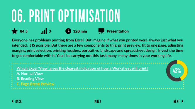
Everyone has problems printing from Excel. But imagine if what you printed were always just what you intended. It IS possible. But there are a few components to this: print preview, fit to one page, adjusting margins, print selection, printing headers, portrait vs landscape and spreadsheet design. Invest the time to get comfortable with it. You'll be carrying out this task many, many times in your working life.

Which Excel 'View' gives the clearest indication of how a Worksheet will print?A. Normal ViewB. Reading ViewC. Page Break Preview

06. Print Optimisation84.5 3 120 min Presentation

Back NextIndex

The beauty of Excel is its easy scalability. Get the formula right once and Excel will churn out the right calculation a million times. The + cross hair is handy. Double clicking it will take it all the way down if you have continuous data. Sometimes a copy and paste (either regular paste or paste formulas) will be faster for you.

07. Extend formula across/down84.1 1 5 min Orientation & Efficiency

Back NextIndex

Excel developed a mind of its own in 2013. Say you have two columns of names and you need to construct email addresses from them all. Just do it for the first row and Excel will work out what you mean and do it for the rest. Pre-2013 this was possible but relied on a combination of functions (FIND, LEFT, &, etc). Now this is much faster and WILL impress people. If Flash Fill is turned on (File Options Advanced) it should just start working as you type. Or get it going manually by clicking Data > Flash Fill, or Ctrl E.

08. Flash Fill83.6 2 30 min Data Handling

Back NextIndex

This is one of the most powerful combinations of Excel functions. You can use it to look up a value in a big table of data and return a corresponding value in that table. Let's say your company has 10,000 employees and there's a spreadsheet with all of them in it with lots of information about them like salary, start date, line manager etc. But you have a team of 20 and you're only really interested in them. INDEX-MATCH will look up the value of your team members (these need to be unique like email or employee number) in that table and return the desired information for your team. It is worth getting your head around this as it is more flexible and therefore more powerful than VLOOKUPs.

09. INDEX-MATCH81.9 4 45 min Data Analysis

Back NextIndex

Explore data in a table quickly. Filtering effectively hides data that is not of interest. Usually there's a value e.g. 'Blue cars' that you're looking for and Filters will bring up those and hide the rest. But in more modern versions of Excel, you can now also filter on number values (e.g. is greater than, top 10%, etc), and cell colour. Filtering becomes more powerful when you need to filter more than one column in combination e.g. both colours and vehicles to find your blue car. Alt D F F is the shortcut (easier than it sounds - give it a go). Conditional Formatting and Sorting serve related purposes. Sorting involves rearranging your spreadsheet, which is intrusive and may not be desirable. Conditional formatting brings visualisation. Filtering is fast and effective. Choose well.

10. Filters81.3 2 60 min Data Handling

Back NextIndex

Used to add numbers up quickly. Note there's Autosum as well and the shortcut Alt +. One problem people face is when you're summing over some values with errors. See IF(ISERROR()) in this list.

11. SUM81.0 0 2 min Foundation

Back NextIndex

Undoing mistakes is hard in life but easy in Excel. There's a curved backwards arrow in the top left of modern versions of Excel. Or easier still Ctrl Z. It pairs nicely with Redo (Ctrl Y) as you try to hone in on exactly the place you want to get back to.

12. Ctrl Z81.0 0 1 min Foundation

Back NextIndex

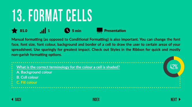
Manual formatting (as opposed to Conditional Formatting) is also important. You can change the font face, font size, font colour, background and border of a cell to draw the user to certain areas of your spreadsheet. Use sparingly for greatest impact. Check out Styles in the Ribbon for quick and mostly non-garish formatting options.

What is the correct terminology for the colour a cell is shaded?A. Background colourB. Cell colourC. Fill colour

13. Format Cells81.0 1 5 min Presentation

Back NextIndex

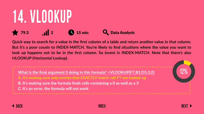
Quick way to search for a value in the first column of a table and return another value in that column. But it's a poor cousin to INDEX-MATCH. You're likely to find situations where the value you want to look up happens not to be in the first column. So invest in INDEX-MATCH. Note that there's also HLOOKUP (Horizontal Lookup).

What is the final argument 0 doing in this formula? =VLOOKUP(F7,B1:D5,3,0)A. It's making sure only entries that EXACTLY match cell F7 are looked upB. It's making sure the formula finds cells containing a 0 as well as a 3C. It's an error, the formula will not work

14. VLOOKUP79.3 2 15 min Data Analysis

Back NextIndex

Shortcut for copying quickly. Goes together with Ctrl V (pasting), like a horse and carriage. Ctrl X is the shortcut for cutting (moving) data around. Sometimes this is what you need instead.

15. Ctrl C79.3 0 1 min Foundation

control + C

Back NextIndex

Shortcut for pasting quickly. Preceded, almost always, by Ctrl C (copy).

16. Ctrl V79.3 0 1 min Foundation

control + V

Back NextIndex

Add (+), subtract (-), multiply (*), divide (/). You'll also need to use brackets sometimes. For example, if cell A1 is 35, cell A2 is 50 and you want to calculate the % increase from 35 to 50 in cell A3, it's '=(A2-A1)/A1'. Without the brackets your answer would be wrong. Remember BODMAS?

What does the character ^ do in an Excel formula?A. Raises a quantity to a power (e.g. 3^2 is 3-squared)B. Reformat the characters following it as a superscriptC. Force characters following it to be interpreted as text rather than a number

17. Basic Arithmetic79.3 1 10 min Foundation

Back NextIndex

COUNT counts numbers, not words. Use it if you need a permanent display of how many of a thing there are or if you need it for other dependent calculations. Almost as useful is COUNTA which counts any text, numbers or string but not blanks. Note that for many purposes the status tray (in the bottom right-hand corner) with count enabled will suffice.

18. COUNT and COUNTA78.4 1 5 min Data Analysis

Back NextIndex

Does exactly what you'd expect. Often safer and better to grab the full array, paste them as values in another sheet / workbook and then apply Remove Duplicates. Tells you how many items got removed. Useful to have an idea of how many removals there should be. A milder variation of this is Highlight Duplicates which is one of the options in Conditional Formatting.

19. Remove Duplicates78.4 2 10 min Data Handling

Back NextIndex

Counts cells with certain properties. Properties include: being a certain number or word (most useful), being above/below certain values, being an error.

20. COUNTIF78.4 2 15 min Data Analysis

Back NextIndex

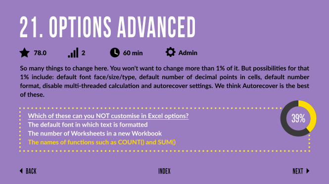
So many things to change here. You won't want to change more than 1% of it. But possibilities for that 1% include: default font face/size/type, default number of decimal points in cells, default number format, disable multi-threaded calculation and autorecover settings. We think Autorecover is the best of these.

Which of these can you NOT customise in Excel options?The default font in which text is formattedThe number of Worksheets in a new WorkbookThe names of functions such as COUNT() and SUM()

21. Options Advanced78.0 2 60 min Admin

Back NextIndex

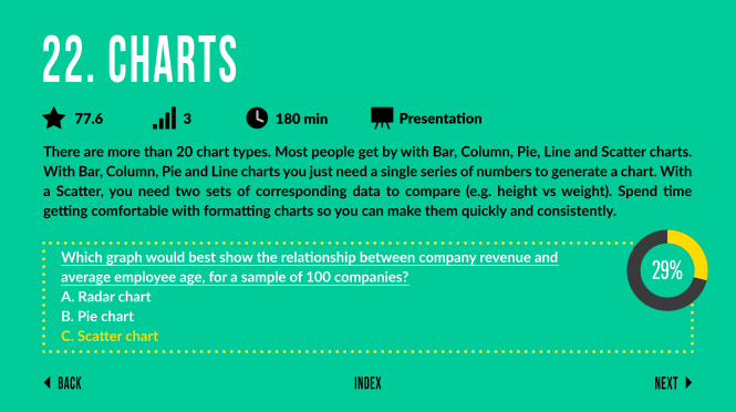
There are more than 20 chart types. Most people get by with Bar, Column, Pie, Line and Scatter charts. With Bar, Column, Pie and Line charts you just need a single series of numbers to generate a chart. With a Scatter, you need two sets of corresponding data to compare (e.g. height vs weight). Spend time getting comfortable with formatting charts so you can make them quickly and consistently.

Which graph would best show the relationship between company revenue andaverage employee age, for a sample of 100 companies?A. Radar chartB. Pie chartC. Scatter chart

22. Charts77.6 3 180 min Presentation

Back NextIndex

Enables you to always see a certain number of columns or rows. Usually this will just be the very top row or two. Sometimes it's helpful to have a column or two as well. Alt W F is the shortcut. You can also split windows and move around in each but this is disorienting for most people - freezing is better! Use 'Unfreeze Panes' to undo this.

23. Freeze Panes77.6 1 15 min Orientation & Efficiency

Back NextIndex

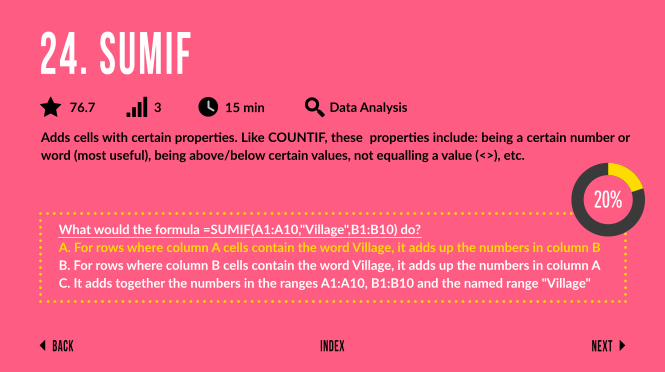
Adds cells with certain properties. Like COUNTIF, these properties include: being a certain number or word (most useful), being above/below certain values, not equalling a value (<>), etc.

What would the formula =SUMIF(A1:A10,"Village",B1:B10) do?A. For rows where column A cells contain the word Village, it adds up the numbers in column BB. For rows where column B cells contain the word Village, it adds up the numbers in column AC. It adds together the numbers in the ranges A1:A10, B1:B10 and the named range "Village"

24. SUMIF76.7 3 15 min Data Analysis

Back NextIndex

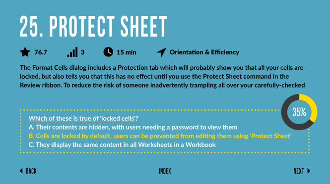
The Format Cells dialog includes a Protection tab which will probably show you that all your cells are locked, but also tells you that this has no effect until you use the Protect Sheet command in the Review ribbon. To reduce the risk of someone inadvertently trampling all over your carefully-checked

Which of these is true of 'locked cells'?A. Their contents are hidden, with users needing a password to view themB. Cells are locked by default, users can be prevented from editing them using 'Protect Sheet'C. They display the same content in all Worksheets in a Workbook

25. Protect Sheet76.7 3 15 min Orientation & Efficiency

Back NextIndex

These are two great uses of the F4 function: 1. Repeats the last action. Say you just inserted three rows and you want another three...just press F4. 2. Toggles through the various combinations of dollar signs for rows and columns, i.e. your Absolute References. It is said that this is the most frequently used shortcut in the whole of Excel. If you only learn one, learn this one!

26. F476.7 1 10 min Orientation & Efficiency

Back NextIndex

Reorder a table of data by the data in one of the columns (e.g. Spend). Very quickly you can draw out patterns and insights. Create a hierarchy of prioritising criteria by first sorting one column and then another (e.g. first by Spend and then by Sales). Occasionally it's useful to sort from left to right according to the values along a row. Take care to be clear about whether your data has row headings. And if you have some referencing formulas going up and down your spreadsheet (e.g. INDEX-MATCHES) they are likely to be rendered useless.

27. Sort75.4 2 30 min Data Handling

Back NextIndex

Save As, fast. This is a more useful shortcut than Ctrl S as Autosave should have you covered for saving a file as is. Save As is useful for version control e.g. you want to keep your current file but create a fork in the road for the latest version. Use Ctrl Shift S to make your Save As that bit faster.

28. Save As (F12)75.4 0 1 min Admin

Back NextIndex

Move a column by clicking on the letter(s) at the top then hover over the edge of the highlighted row and drag and drop it left or right. Ditto for rows. If you want a copy of that column (or row) hold Ctrl as you do the drag and drop. If you haven't seen this before, try it now, for a column.

29. Move or Copy Column / Row75.0 1 10 min Orientation & Efficiency

Back NextIndex

Jumps you from current active cell to the last populated cell in whichever direction you've specified (North, South, East, West). Ctrl Home takes you to A1. Ctrl End takes you to the last (most South-Easter-ly, as it were) used cell in the spreadsheet.

30. Ctrl (Arrows, Pg Up, etc)74.6 0 5 min Orientation & Efficiency

Back NextIndex

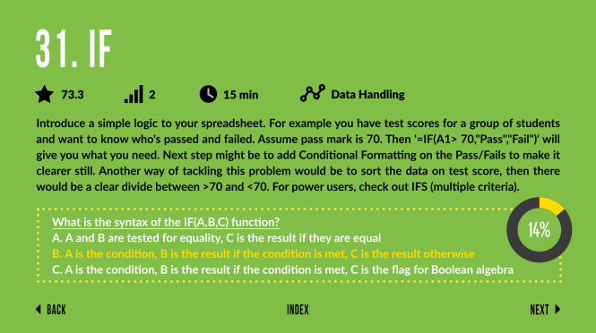
Introduce a simple logic to your spreadsheet. For example you have test scores for a group of students and want to know who's passed and failed. Assume pass mark is 70. Then '=IF(A1> 70,"Pass","Fail")' will give you what you need. Next step might be to add Conditional Formatting on the Pass/Fails to make it clearer still. Another way of tackling this problem would be to sort the data on test score, then there would be a clear divide between >70 and <70. For power users, check out IFS (multiple criteria).

What is the syntax of the IF(A,B,C) function?A. A and B are tested for equality, C is the result if they are equalB. A is the condition, B is the result if the condition is met, C is the result otherwiseC. A is the condition, B is the result if the condition is met, C is the flag for Boolean algebra

31. IF73.3 2 15 min Data Handling

Back NextIndex

A nice use of Excel's logical capability is the = feature, set between two cells. This will return TRUE if A1 is equal to B1 and FALSE otherwise. A great use of this is to check that numbers in different areas of your spreadsheet that should calculate the same number are in fact doing so. For example, in a financial model you might have two ways of building up to a forecast revenue figure. Using the equals sign in this way can check for any errors. It might even be worth having a dashboard of error checking values (maybe spruced up with some conditional formatting) to ensure that everything's working as it should.

32. Linking Cells (eg '=A1=B1')73.3 1 5 min Admin

Back NextIndex

Fit all your text in the cell. A clear advantage is that you can read it all. A disadvantage is that it may make your spreadsheet less attractive with varying column widths and/or row heights. A way of combatting that is to wrap and standardise the column widths or row heights by highlighting them all and then setting a fixed common width/height.

33. Wrap Text73.3 2 15 min Data Handling

Back NextIndex

Errors (#VALUE!, #####, #DIV/0!, #REF!, etc) look ugly and can stop calculations working (e.g. summing over a range of values with a single #DIV/0!). You can avoid it by using '=IF(ISERROR())'. This combination of functions will put a value (for blanks, entering "" should work) if there's an error and just whatever the calculated value is otherwise e.g. =IF(ISERROR(E25),"",E25).

34. IF and ISERROR73.3 2 30 min Data Handling

Back NextIndex

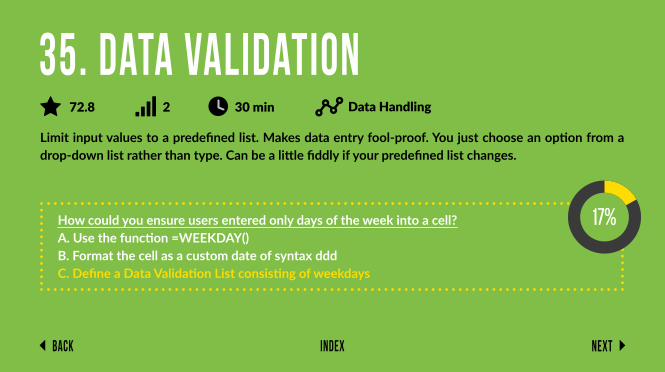
Limit input values to a predefined list. Makes data entry fool-proof. You just choose an option from a drop-down list rather than type. Can be a little fiddly if your predefined list changes.

How could you ensure users entered only days of the week into a cell?A. Use the function =WEEKDAY()B. Format the cell as a custom date of syntax dddC. Define a Data Validation List consisting of weekdays

35. Data Validation72.8 2 30 min Data Handling

Back NextIndex

Sometimes you type what looks to Excel like the start of a formula. If the first character is +, -, = etc, Excel treats the cell differently and starts looking for cells to refer to. This can be disorienting. Simply putting an apostrophe at the start of the cell puts a stop to all that and it won't appear in the cell (try it!) Also works if you have some zeros at the start of a number (eg 0099) which you want to keep.

36. Use of ' (apostrophe)72.8 1 5 min Data Handling

Back NextIndex

There are two ways you can do this.

1. Right Click on a column (or row) and select column width if you know the exact value of the width (or height for rows) you want. 2. Hover over the edge of the column (or row) and drag to the width (height) you want.

Having consistent column widths will improve the look of your spreadsheet. Highlighting the columns and applying either of the above methods achieves that efficiently.

37. Resize Columns / Rows72.4 1 5 min Orientation & Efficiency

Back NextIndex

Activates selected cell for editing by taking you into the formula bar at the top. Saves you clicking there with the mouse. Surprisingly useful and many Excel users' favourite shortcut.

38. F272.4 1 2 min Orientation & Efficiency

F2

Back NextIndex

Gives you a line break within an individual cell. Can be used to depict bullet points within a cell (note that if you want to open with a '-' bullet you'll need the apostrophe before it or else Excel will think you're trying to create a formula). Generally this trick can be used to make the information in the cell stand out more clearly.

39. Alt Enter72.4 1 2 min Orientation & Efficiency

+alt enter

Back NextIndex

These can be frustrating for a lot of Excel users. Turning ordinary-looking dates into long strings of seemingly meaningless numbers and ###### errors. Get on top of these once and for all by defining a custom number format set and knowing where that is. We recommend having commas separating thousands, a sensible number of decimal places (usually 0, 1, or 2) and using '-' for blanks and negative numbers in red and in brackets. Here's an example: #,##0_);[Red](#,##0);-?. You'll have your own preferences.

40. Number Formats72.4 1 30 min Presentation

Back NextIndex

A good job is getting your spreadsheet to a professional standard: consistent formatting, orientated, printer friendly, spreadsheet checks, etc. A great job is telling your story: the right cells should stand out and remain so as numbers update. This is great layout, design and formatting. Aspire to that.

41. Layout, Design & Formatting71.1 3 120 min Presentation

Back NextIndex

The opposite of Ctrl Z and works brilliantly with Ctrl Z to hone in on exactly the stage of your work you want to get back to.

42. Redo (Ctrl Y)71.1 1 2 min Orientation & Efficiency

control + Y

Back NextIndex

Suppose we have some monthly marketing costs in a spreadsheet, set out vertically, from cell B3 down. And suppose we want to know how much we have cumulatively spent in any given month of the year, so that we can see at what point we hit a certain budget level e.g. £500k. This formula does what we need beautifully as we enter into cell C3, say: '=SUM($B$3:B3)'. Then just extend the formula down column C as far as you need to. Try it!

43. Cumulative Sum71.1 1 10 min Data Analysis

Back NextIndex

1. Find, using the shortcut Ctrl F. This will find you some text within any cell in your spreadsheet.2. Together with Replace, change the string for a different string e.g. changing 'APPLES' to 'ORANGES'.

Beware of Replace - unintended consequences are very likely with this feature! For example, suppose you had some apples in your spreadsheet (as it were) and you wanted to change them to oranges. That's fine if all you have is apples. But if you had some pineapples too you'd end with some pineoranges. Inter-esting concept but probably not what your spreadsheet needs. Avoid using replace in large spread-sheets in which unintended consequences are hard to see.

Like Remove duplicates, Excel will tell you how many replacements have been made - try to have an idea of what number this should be so you can sense check.

44. Find and Replace70.7 1 15 min Orientation & Efficiency

Back NextIndex

Combines the contents of cells together. So along your first row if you have Mr in A1, James in B1 and Smith in C1, '=A1&B1&C1' will give you MrJamesSmith. =A1&" "&B1&" "&C1 gives Mr James Smith. But note that & is usually enough. If you need to combine many cells, CONCATENATE may be faster.

45. & and CONCATENATE70.7 1 15 min Data Handling

Back NextIndex

Just as Ctrl Up-Arrow will take you quickly up your spreadsheet (up to the next stopping point), Ctrl Shift Arrow will highlight all the cells from the one currently selected up to the stopping point. Works very nicely with copying and pasting a bunch of values.

46. Extend Selection70.7 1 10 min Orientation & Efficiency

Back NextIndex

PivotTable slicers do the same thing as Filters - they enable you to show certain data and hide other data as required. But rather than dull drop-down menus, slicers offer nice big friendly buttons to make the whole user experience nicer and easier. As well as fast filtering, slicers also tell you what the current filtering state is so you know what's currently in and out of the PivotTable report.

47. Slicers70.7 2 45 min Data Analysis

Back NextIndex

Try it but just make sure you have at least two Excel files open when you do!

48. Ctrl Tab70.7 1 2 min Orientation & Efficiency

control + tab

Back NextIndex

Returns the maximum or minimum value from a range of cells. Conditional formatting and sorting your data are also ways in which you can find these values. This is just a bit faster. Useful as a quick check that in a huge set of data all the values are within a sensible, realistic range. (Note that you can get maximum and minimum values from the status bar tray in the bottom right-hand corner, too.)

49. MAX, MIN70.3 1 15 min Data Analysis

Back NextIndex

If you want to say something about a cell or some cells in a spreadsheet, insert a Comment. This is espe-cially useful for shared documents when you're leaving comments for others. But they can get messy quickly when they're shown and don't do much good when they're hidden. They get even messier if you move rows / columns around with the comments in. So use it sparingly and try to incorporate all data into your spreadsheet. Shortcut is Shift F2.

50. Comments69.8 1 15 min Data Handling

Back NextIndex

Calculates or predicts a future value by using existing values. You can use this function to predict future sales, inventory requirements or consumer trends. From Excel 2016 onwards.

51. FORECAST69.0 2 120 min Data Analysis

Back NextIndex

You can insert almost any symbol. But in our experience, the ones you're most likely to need are: tick, cross and star. These especially useful symbols are all available in Wingdings, best accessed with Insert Symbol.

52. Insert Symbols69.0 1 10 min Presentation

Back NextIndex

Looks for a given string from within a cell and tells you if it can be found. For example, if you had a thou-sand email addresses and you wanted to know how many of them were Gmail, you would use Find to tell you for each email whether the string 'Gmail' appears or not. Then count the results (see COUNT, elsewhere on this list) or use Conditional Formatting to bring these out. Note that FIND is case sensi-tive; Search is a non-case-sensitive alternative.

53. FIND69.0 1 15 min Data Handling69.0 1 15 min Data Handling

Back NextIndex

You can put a lot in here, including calculations (Maximum, Minimum, Average, Sum, Count), keyboard status (Caps Lock, Num Lock, Scroll Lock) and others. Pick what you need. We recommend Sum, Count and Average only. You'll see the values appear as you select multiple cells with relevant values.

54. Customise Status Bar69.0 1 10 min Orientation & Efficiency

Back NextIndex

LEN is perhaps the most useful for returning the number of characters in a cell, and can be used to determine, for example, if your copy is too long or too short for a tweet (140 characters). The others (LEFT/MID/RIGHT) take portions of text from a string in a cell. These four functions work well together (and also FIND which is number 53 on this list and TRIM, which sadly didn't quite make it) to manipulate text into the format you need (eg an email address). For the more advanced user, here's a formula to count the WORDS in a cell: '=IF(LEN(TRIM(A2))=0,0,LEN(TRIM(A2))-LEN(SUBSTITUTE(A2," ",""))+1)'. Try!

55. LEN (and LEFT/MID/RIGHT)68.8 3 30 min Data Handling

Back NextIndex

Calculates the mean average of a list of values. Note the lighter touch alternative of highlighting the numbers you're interested in and looking at the status tray at the bottom of your screen.

56. AVERAGE68.1 1 5 min Data Analysis

Back NextIndex

Start typing out a formula e.g. '=SUMIF(' and then hit Ctrl Shift A. You'll then see =SUMIF(range, criteria, sum_range) in the Formula Bar (a hint for what cell ranges should be put where). Only useful for the more complicated functions, obviously.

57. Ctrl Shift A68.1 2 10 min Data Handling

control + shift + A

Back NextIndex

What-If Analysis is a set of tools that take an input value and determine the result. It is the process of changing values in cells to see how those changes will affect the outcome of formulas on the worksheet. One of those tools is Goal Seek. If you know the result that you want from a formula, but are not sure what input value the formula needs to get that result, use the Goal Seek feature. From Excel 2010 onwards.

58. Goal Seek / What If67.7 4 120 min Data Analysis

Back NextIndex

Do this by clicking the top-most, left-most grey box. It is to the left of the letters and above the numbers. Ctrl A does a similar thing but with a subtle difference: if the cursor is in an empty cell, Ctrl A selects the entire worksheet; if you're in a group of connected cells, Ctrl A will select that group of cells instead. Useful when you want to change the formatting for your whole sheet in one go (e.g. make everything the same font size).

59. Select All67.7 1 10 min Orientation & Efficiency

Back NextIndex

When troubleshooting or trying to make sense of formulas, it's useful to be able to display the relation-ships between formulas and cells. To assist you in checking your formulas, you can use the Trace Prece-dents and Trace Dependents commands to graphically display, or trace the relationships between these cells and formulas with tracer arrows. From Excel 2007 onwards.

Which of the following is a Formula Auditing option?A. Reconcile TotalsB. Trace PrecedentsC. Conditional Formatting

60. Precedents & Dependents66.8 3 30 min Data Handling

Back NextIndex

Change the case of text from all upper, to sentence, or all lower case. Useful for changing names into the format you might need for sending out lots of emails, letters, etc. Or just to make your spreadsheet look more consistent.

61. UPPER, PROPER, etc65.1 2 180 min Data Handling

Back NextIndex

Powerful feature which brings a lot more firepower to PivotTables (e.g. COUNTROWS) and more processing power to deal with much larger data sets. Mostly for Excel experts and BI professionals.

62. PowerPivots64.2 4 180 min Data Analysis

Back NextIndex

Go to File then New on the modern versions of Excel and you'll see a range of templates. There's a Gantt chart, various dashboards, calendars, cash flows, inventories and much more. They're pretty. Maybe none of these will be 100% perfect for your specific needs. But take and tweak - that's one of the major benefits of Excel. Using and adapting these templates will also open your eyes up to design possibilities in Excel.

63. Templates64.2 3 30 min Presentation

Back NextIndex

The Ribbon is wonderful but what's shown on it responds to what you're doing on the spreadsheet. That's why it's wonderful. But there may be some features you use so frequently that you want them to be there always. Maybe you sort data a lot. Then add it to the Quick Access Toolbar, right at the top of your screen. But note that for any action you carry out many times, you may prefer to learn and use the shortcut.

64. Quick Access63.8 1 30 min Orientation & Efficiency

Back NextIndex

Brings up available print options. Printing is a bugbear for the majority of Excel users. This is a small part of that. See Print Optimisation, further down at number 6.

65. Ctrl P62.5 0 1 min Presentation

control + P

Back NextIndex

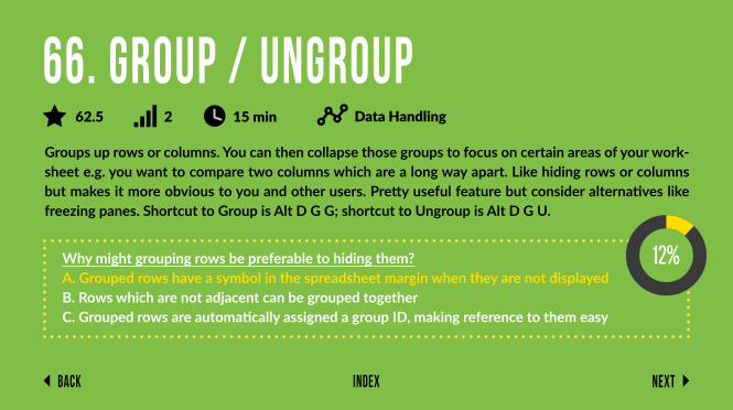
Groups up rows or columns. You can then collapse those groups to focus on certain areas of your work-sheet e.g. you want to compare two columns which are a long way apart. Like hiding rows or columns but makes it more obvious to you and other users. Pretty useful feature but consider alternatives like freezing panes. Shortcut to Group is Alt D G G; shortcut to Ungroup is Alt D G U.

Why might grouping rows be preferable to hiding them?A. Grouped rows have a symbol in the spreadsheet margin when they are not displayedB. Rows which are not adjacent can be grouped togetherC. Grouped rows are automatically assigned a group ID, making reference to them easy

66. Group / Ungroup62.5 2 15 min Data Handling

Back NextIndex

Been here for a decade now, the fluent user toolbar aka Ribbon. It responds to what you're doing, show-ing you more relevant functions and features as you use Excel. It's customisable too.

67. Customising the Ribbon62.5 1 15 min Admin

Back NextIndex

Saves your work. This is of course important. But it's arguably even more important to get your Autosave and Autorecover settings (accessible through Excel Options) right and be less reliant on manual saving. Note also that Save As will sometimes be better if you want to save a new version of the file (eg as a v2).

68. Ctrl S62.5 0 1 min Admin

control + S

Back NextIndex

A Sparkline is a tiny chart in a worksheet cell that provides a visual representation of the data selected. Sparklines are useful for showing trends in a series of values, such as seasonal increases or decreases, economic cycles, or to highlight maximum and minimum values. Sparklines can be displayed as lines or columns and can also represent any negative values. Position a Sparkline near its data for greatest impact. From Excel 2010 onwards.

69. Sparkline62.1 2 15 min Data Analysis

Back NextIndex

Duplicate a worksheet by pressing and holding Ctrl and dragging the desired tab to the right. If you look closely an icon with a crosshair will appear. You'll probably then want to change the tab name so this combines nicely with double clicking on your newly created tab to rename.

70. Copy-Drag Worksheet62.1 0 2 min Orientation & Efficiency

Back NextIndex

If you have tasks in Excel that you need to do repeatedly, you can record a macro to automate those tasks. A macro is an action or a set of actions that you can run as many times as you want. When you create a macro, you are recording your mouse clicks and keystrokes. The macro can then be saved and run whenever it is needed. Macros can also be edited to make minor changes to the way it works. From Excel 2007 onwards.

71. Macros & VBA62.1 4 60 min Data Analysis

Back NextIndex

A basic logical function which requires more than one condition to hold. Returns TRUE if all conditions are met and FALSE otherwise. Useful, for example, if you want to identify quickly all the blue cars in a database (where one column has vehicle data and another has colour data). Works well with conditional formatting (e.g. highlighting the TRUEs) and sorting. But you'll often find that a simple filter (on multiple columns) at the outset will do what you need.

72. AND62.1 1 5 min Data Handling

Back NextIndex

You display your text at any angle. You can even display each letter vertically on top of the other (like, for example, the iconic neon Radio City sign in New York). Sometimes useful but it's hard to read so consid-er alternatives like increasing row height, wrapping the text and adjusting column width to suit.

73. Rotate Text61.6 1 10 min Presentation

Back NextIndex

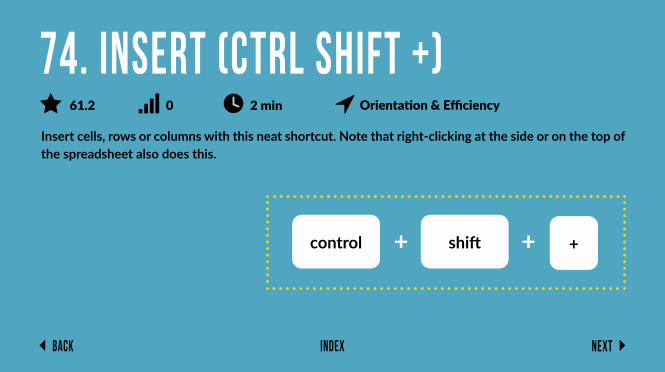
Insert cells, rows or columns with this neat shortcut. Note that right-clicking at the side or on the top of the spreadsheet also does this.

74. Insert (Ctrl Shift +)61.2 0 2 min Orientation & Efficiency

control + shift + +

Back NextIndex

Excel will automatically change certain text inputs, assuming you've made a mistake e.g. the letter c in brackets is corrected to the copyright symbol. That won't always be right. So review the list if Excel autocorrects too much for your liking, or you have some text you're inputting repeatedly which is becoming a drag (e.g. changing 'esb' to Empire State Building).

75. Autocorrect61.2 3 10 min Admin

Back NextIndex

This menu gives a lot of options. Maybe too many! Most useful of these is probably Hyperlink as the others (e.g. sorting and filtering) are easily and more intuitively activated in other ways.

76. Right-Click on Cell60.3 0 10 min Orientation & Efficiency

Back NextIndex

Adds the numbers above or to the side. Shortcut is 'Alt ='.

77. AutoSum (Alt =)60.3 0 2 min Foundation

+alt =

Back NextIndex

Separate out combined data e.g. 'Chapman, Tracy' all in a single cell, into two cells e.g. 'Chapman' in one cell and 'Tracy' in the next cell. Much faster than using FIND, LEN, LEFT, etc, to carry this out which was the only option before Microsoft introduced this feature.

To do it: highlight your data, click on the Data tab in the Ribbon and choose Text to Columns.

78. Text to Columns60.3 1 30 min Data Handling

Back NextIndex

Highlights entire selected column. Fast.

79. Ctrl Space59.5 0 2 min Orientation & Efficiency

control + space

Back NextIndex

Want some random dummy data to make your spreadsheet look full? RANDBETWEEN will give you random numbers between any two values you specify. For example, =RANDBETWEEN(1,100) will give you random percentages. There's also RAND which will give you a random number between 0 & 1 to many decimal places.

80. RANDBETWEEN59.5 2 15 min Data Analysis

Back NextIndex

Excel Tables were introduced in Excel 2007. Don't ever believe they're just about fancy formatting. The real power of Tables is that they expand automatically when you add data in the row immediately beneath existing rows, or the column immediately to the right of existing columns. This means that formula references to entire Table columns can expand automatically to include new data. Excel objects such as PivotTables and Charts based on Tables can also include new rows, and columns, without need-ing to change the data source manually. Tables have their own ribbon tab where you can give them a descriptive name, turn on a Total Row and do lots of other useful stuff like including a Filter Button in each heading cell.

81. Tables59.5 3 60 min Data Handling

Back NextIndex

A Named Range is one or more cells that have been given a name by the user. Using named ranges instead of row and column references can make formulas easier to read and understand. Warning: some people (especially Excel beginners) find them MORE confusing!

What would have to have been set before the formula =SUM(Grid) would work?A. A function called Grid, referring to some cellsB. An absolute reference called Grid, referring to some cellsC. A named range called Grid, referring to some cells

82. Named Ranges / Name Manager58.6 3 45 min Data Handling

Back NextIndex

Double click on the worksheet tab at the bottom of your spreadsheet. Niftier than the alternative (Right click and select Rename). We've included it in our list because it's a very common thing we all do.

83. Double Click to Rename Sheet58.2 1 1 min Orientation & Efficiency

Back NextIndex

There are more than 20 Time and Date functions. But probably the most useful application for most of us is manipulating dates. For example, if you have a date in cell A1 and a later date in cell B1, '=B1-A1' will tell you how many days were in between. =(B1-A1)/365) will tell you how many years are in between. Or, using the same example, type in cell A2 '=A1+7) and drag down. You'll have a long list of dates, one week apart.

84. Date and Time Functions58.2 2 30 min Data Handling

Back NextIndex

Trivial to many, impossible to some. Let's say cell A1 has the value 25, and A2 is 40. What's the % growth from A1 to A2? It's '=(A2-A1)/A1%'. Even that's not super-clear to everyone. But it's even harder going the other way around - what's the formula to calculate the % reduction from 40 to 25?

85. Calculate Discounts / Growth57.8 2 5 min Data Analysis

Back NextIndex

Cool one. Click on a cell which has the formatting you desire. Then double click on the Format Painter icon under Home. You can then paint that formatting to as many cells or groups of cells for as long as you like.

86. Double Click Format Painter57.8 1 2 min Presentation

Back NextIndex

Create a timeline such as a Gantt Chart in Excel to help manage a project, display your expenses, sched-ule a series of events, etc. They look nice and respond to data changes helpfully and intuitively. There are lots of templates online including some nice ones from Smartsheet here: ttps://www.smartsheet.com/blog/how-make-excel-timeline-template.

What is a Timeline?A. A curve fitted to a set of data in an Excel chartB. A log of Excel activity to allow actions to be undone or redoneC. A graphical way of filtering by date in a PivotTable

87. Timeline57.8 2 30 min Data Analysis

Back NextIndex

Adds a new, empty workbook to your Excel file. Note that if you want any of the formatting or values from an existing sheet, you may want to duplicate one of the existing tabs.

88. New Workbook (Shift-F11)57.8 0 2 min Orientation & Efficiency

Back NextIndex

Not all that useful all that often. But feels nice when you can use it and remember it. The shortcuts for underlining (Ctrl U) and emboldening (Ctrl B) are easier to remember. Which is why fewer people know Ctrl 5. So you'll be in an exclusive group!

89. Ctrl 5 (Strikethrough)56.7 0 2 min Orientation & Efficiency

Back NextIndex

Converts a reference assembled as text e.g. 'Sheet1!A1' into a proper reference. So Excel knows to find the value from the cell in A1 rather than treat it as text.

90. INDIRECT56.0 4 15 min Data Handling

Back NextIndex

Italicise (Ctrl I) or embolden (Ctrl B) text quickly and easily. Incidentally, Ctrl 3 and Ctrl 4 do the same thing. But they're hard to remember. Note that if you have multiple cells to italicise/embolden, clicking them all separately as you press and hold Ctrl and then hit I or B, you'll have formatted your spreadsheet very efficiently.

91. Italicise and Embolden56.0 0 1 min Orientation & Efficiency

Back NextIndex

Do not confuse the number of decimal places you can see displayed in a cell with the number that will be used in a calculation using the value in that cell! When you decrease the number of decimals displayed in a cell, only the displayed value is rounded. Unless you have turned on Precision as Displayed option, the full precision of your value will still be used in calculations. This can cause apparent rounding issues. Just type 1.5, 2.5 and 3.5 into cells A1 to A3, use SUM() in A4 then change the display to show no decimal points. So if you really want your values to be treated as 2, 3 and 4 you need to use the ROUND() function. The first argument is the value to be rounded and the second the number of decimal points. For example: =ROUND(A1,0). Use ROUND() to round each of your 3 values to no decimal points and then see what the sum is.

92. Rounding56.0 2 10 min Data Handling

Back NextIndex

Waterfalls plot the ongoing cumulative result of a series of values. They work especially well when telling a story of interventions (and their numerical effects) over time (e.g. the overall and interim effects of a series of recruitment strategies on employee count).

93. Waterfall Chart55.2 1 30 min Presentation

Back NextIndex

Cell references are usually in 2 dimensions – columns and rows. It is possible to create a reference that adds a third dimension by looking through the worksheets in a workbook. Suppose you have sales data for Year 1 in worksheet 1, Year 2 in worksheet 2 and so on. Then you can sum across the worksheets, in a 'third dimension' (beyond the usual two: rows & columns), hence the name. If you want to add up all the cells in B5, for instance the formula is '=SUM(Sheet1:Sheet3!B5)'. Just make sure that all the work-sheets are and remain identically structured.

94. 3d SUM55.2 1 15 min Data Analysis

Back NextIndex

Data that you want to use in Excel might not always be stored in another Excel workbook. Sometimes that data may exist externally (e.g. in an access file), in a database or maybe on the web. This data can be imported into Excel easily using the 'Get External Data' utility. The main benefit of connecting to exter-nal data is that you can periodically analyse it in Excel without having to repeatedly copy it which can be time consuming and error prone. From Excel 2010 onwards.

95. Get External Data (from Web)54.3 4 45 min Data Analysis

Back NextIndex

Use the shortcut or select the Formulas tab, then click Show Formulas located in the Formula Auditing group. Useful if you quickly want to check whether there are formulas in the spreadsheet and also to check if they look right.

96. Show Formulas (Ctrl ¬)54.3 1 2 min Data Handling

Back NextIndex

Another quick and easy tip - note that with all the horizontal lines that naturally appear in Excel, under-lining is less visually effective. (Ctrl 4 does the same thing but Ctrl U is easier to remember so stick with that).

97. Ctrl U (Underline)53.9 0 1 min Orientation & Efficiency

+ Ucontrol

Back NextIndex

This is a free text search bar in which you use natural language to get to the right function feature. For example, if I type, 'Change colour of cell', both format cells and font colour come up as options. Useful occasionally, when you've just forgotten where the feature is on the Ribbon. From Excel 2016 onwards.

98. Tell me what you want to do53.9 1 15 min Admin

Back NextIndex

Select a cell and hit Shift Space on your keyboard. This highlights the entire row. This works nicely when combined with any action that applies to the whole row eg deleting it (Ctrl 9), colouring it, resizing it, etc. An alternative to this is just to click on the row number on the left hand side of your spreadsheet.

99. Shift Space53.4 0 2 min Orientation & Efficiency

Back Index

Ctrl 9 (delete current row) & Ctrl 0 (delete current column). Very quick and efficient. But note this is a fraction slower (and more time consuming to spot if it's not the right move) than right clicking on the top of the column, or the left-side of the row.

100. Delete Row (Ctrl 9)53.4 0 2 min Orientation & Efficiency

+control 9

If you're interested in the full, algorithmically personalized Excel course of 160 modules please be in touch: sales@excelwithbusiness.com.

Thanks to Deborah Ashby and Simon Hurst for their expert input. www.excelwithbusiness.com© Excel With Business 2017, all rights reserved.