AFRL-AFOSR-VA-TR-2016- · PDF filePROGRAM ELEMENT NUMBER 61102F 6. AUTHOR(S) ... neurophysiological models using bifurcation ... made significant progress in understanding the signal

AFRL-AFOSR-VA-TR-2016-0359

Signal Processing, Pattern Formation and Adaptation in Neural Oscillators

Edward LargeCircular Logic LLC399 NW 7TH AvenueBoca Raton, FL 33486-3509

11/29/2016Final Report

DISTRIBUTION A: Distribution approved for public release.

Air Force Research LaboratoryAF Office Of Scientific Research (AFOSR)/RTB2

12/8/2016https://livelink.ebs.afrl.af.mil/livelink/llisapi.dll

a. REPORT

Unclassified

b. ABSTRACT

Unclassified

c. THIS PAGE

Unclassified

REPORT DOCUMENTATION PAGE Form ApprovedOMB No. 0704-0188

The public reporting burden for this collection of information is estimated to average 1 hour per response, including the time for reviewing instructions, searching existing data sources, gathering and maintaining the data needed, and completing and reviewing the collection of information. Send comments regarding this burden estimate or any other aspect of this collection of information, including suggestions for reducing the burden, to Department of Defense, Executive Services, Directorate (0704-0188). Respondents should be aware that notwithstanding any other provision of law, no person shall be subject to any penalty for failing to comply with a collection of information if it does not display a currently valid OMB control number.PLEASE DO NOT RETURN YOUR FORM TO THE ABOVE ORGANIZATION.1. REPORT DATE (DD-MM-YYYY) 29-11-2016

2. REPORT TYPEFinal Performance

3. DATES COVERED (From - To)01 Aug 2012 to 31 Jul 2016

4. TITLE AND SUBTITLESignal Processing, Pattern Formation and Adaptation in Neural Oscillators

5a. CONTRACT NUMBER

5b. GRANT NUMBERFA9550-12-1-0388

5c. PROGRAM ELEMENT NUMBER61102F

6. AUTHOR(S)Edward Large

5d. PROJECT NUMBER

5e. TASK NUMBER

5f. WORK UNIT NUMBER

7. PERFORMING ORGANIZATION NAME(S) AND ADDRESS(ES)Circular Logic LLC399 NW 7TH AvenueBoca Raton, FL 33486-3509 US

8. PERFORMING ORGANIZATIONREPORT NUMBER

9. SPONSORING/MONITORING AGENCY NAME(S) AND ADDRESS(ES)AF Office of Scientific Research875 N. Randolph St. Room 3112Arlington, VA 22203

10. SPONSOR/MONITOR'S ACRONYM(S)AFRL/AFOSR RTB2

11. SPONSOR/MONITOR'S REPORTNUMBER(S)

AFRL-AFOSR-VA-TR-2016-0359 12. DISTRIBUTION/AVAILABILITY STATEMENTDISTRIBUTION A: Distribution approved for public release.

13. SUPPLEMENTARY NOTES

14. ABSTRACTIn this project, we developed a theoretical framework for auditory neural processing and auditoryperception. We modeled the auditory system as a dynamical system consisting of oscillatory networks, andauditory perception as stable dynamic patterns formed in the networks in response to acoustic signals. Wedeveloped GrFNNs, generic models that capture the neurocomputational properties of a family ofneurophysiological models using bifurcation theory. We conducted theoretical analyses of GrFNNs andmade significant progress in understanding the signal processing, pattern formation and plasticity in them.We developed three models that exploit these properties to model important aspects of auditoryneurophysiology and auditory perception: a model of cochlear dynamics, a model of mode-locked neuraloscillation in the human auditory brainstem, and a model of cortical phase locking to auditory rhythms.Future modeling efforts based on canonical dynamical systems could bring us closer to understandingfundamental mechanisms of hearing, communication, and auditory system development15. SUBJECT TERMSNonlinear Dynamics, Auditory Perception, Neural Oscillators

16. SECURITY CLASSIFICATION OF: 17. LIMITATION OFABSTRACT

UU

18. NUMBEROFPAGES

19a. NAME OF RESPONSIBLE PERSONBRADSHAW, PATRICK

Standard Form 298 (Rev. 8/98)Prescribed by ANSI Std. Z39.18

Page 1 of 2FORM SF 298



19b. TELEPHONE NUMBER (Include area code)703-588-8492

Standard Form 298 (Rev. 8/98)Prescribed by ANSI Std. Z39.18

Page 2 of 2FORM SF 298



AFOSR Final Performance Report

Project Title: Signal Processing, Pattern Formation and Adaptation in Neural Oscillators

Award Number: FA9550-12-10388

Start Date:

Program Manager: Dr. Patrick O. Bradshaw

Sensory Information Systems Program

Air Force Office of Scientific Research

Directorate of Chemistry and Biological Sciences

875 North Randolph Street

Suite 325

Arlington, Virginia 22203-1768

E-mail: [email protected]

Phone: (703) 588-8492

Fax: FAX (703) 696-7360

Principal Investigator: Dr. Edward W. Large

President

Circular Logic, LLC

222 Pitkin Street

East Hartford, CT 06108

E-mail: [email protected]

Phone: (860) 282-4215

Fax: (860) 282-4901


mailto:[email protected]

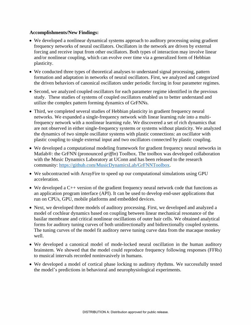
Accomplishments/New Findings:

We developed a nonlinear dynamical systems approach to auditory processing using gradient

frequency networks of neural oscillators. Oscillators in the network are driven by external

forcing and receive input from other oscillators. Both types of interaction may involve linear

and/or nonlinear coupling, which can evolve over time via a generalized form of Hebbian

plasticity.

We conducted three types of theoretical analyses to understand signal processing, pattern

formation and adaptation in networks of neural oscillators. First, we analyzed and categorized

the driven behaviors of canonical oscillators under periodic forcing in four parameter regimes.

Second, we analyzed coupled oscillators for each parameter regime identified in the previous

study. These studies of systems of coupled oscillators enabled us to better understand and

utilize the complex pattern forming dynamics of GrFNNs.

Third, we completed several studies of Hebbian plasticity in gradient frequency neural

networks. We expanded a single-frequency network with linear learning rule into a multi-

frequency network with a nonlinear learning rule. We discovered a set of rich dynamics that

are not observed in either single-frequency systems or systems without plasticity. We analyzed

the dynamics of two simple oscillator systems with plastic connections: an oscillator with

plastic coupling to single external input and two oscillators connected by plastic coupling.

We developed a computational modeling framework for gradient frequency neural networks in

Matlab®: the GrFNN (pronounced griffin) Toolbox. The toolbox was developed collaboration

with the Music Dynamics Laboratory at UConn and has been released to the research

community: https://github.com/MusicDynamicsLab/GrFNNToolbox.

We subcontracted with ArrayFire to speed up our computational simulations using GPU

acceleration.

We developed a C++ version of the gradient frequency neural network code that functions as

an application program interface (API). It can be used to develop end-user applications that

run on CPUs, GPU, mobile platforms and embedded devices.

Next, we developed three models of auditory processing. First, we developed and analyzed a

model of cochlear dynamics based on coupling between linear mechanical resonance of the

basilar membrane and critical nonlinear oscillations of outer hair cells. We obtained analytical

forms for auditory tuning curves of both unidirectionally and bidirectionally coupled systems.

The tuning curves of the model fit auditory nerve tuning curve data from the macaque monkey

well.

We developed a canonical model of mode-locked neural oscillation in the human auditory

brainstem. We showed that the model could reproduce frequency following responses (FFRs)

to musical intervals recorded noninvasively in humans.

We developed a model of cortical phase locking to auditory rhythms. We successfully tested

the model’s predictions in behavioral and neurophysiological experiments.


https://github.com/GrFNN/Toolbox-1.0

Summary:

Many systems in nature, especially biological systems, are nonlinear dynamical systems.

Auditory perception provides a stunning example of just how powerful such systems can be.

Humans recognize complex acoustic patterns under challenging listening conditions, such as a

voice in a crowded room or on a city street. We quickly learn patterns that are significant to us,

such as the sound of a new dog’s bark or the rhythm of a samba. We segregate sounds from one

another, so that we can attend to one sound while suppressing others. These and other

remarkable capabilities of human perception arise from nonlinear dynamical processes in the

auditory system.

We have developed a theoretical framework for auditory neural processing and auditory

perception. Our approach models the auditory system as a dynamical system consisting of

oscillatory neural networks, and auditory perception as stable dynamic patterns formed in the

networks in response to acoustic signals. Our models capture neural dynamics using canonical

dynamical systems. Canonical systems are not detailed neurophysiological models; they are

generic models that capture the neurocomputational properties of a family of neurophysiological

models using bifurcation theory. Such models apply across temporal and spatial scales. For

example, they are appropriate for describing critical nonlinear oscillations of outer hair cells in

the cochlea, mode-locking of chopper cells to sound in the cochlear nucleus, and entrainment of

cortical oscillations to auditory rhythms.

We have made significant theoretical advances in understanding how gradient frequency

neural networks (GrFNNs) respond to acoustic stimulation and how such networks can learn and

adapt through Hebbian plasticity. We analyzed and categorized the driven behaviors of canonical

oscillators under periodic forcing. We conducted series of studies of systems of coupled

oscillators to better understand and utilize the complex network dynamics of GrFNNs. We

completed a comprehensive study of Hebbian plasticity in gradient frequency neural networks.

We discovered a set of rich dynamics that are not observed in either single-frequency systems or

systems without plasticity.

We created a computational modeling framework in Matlab, called the GrFNN Toolbox, and

we have made our models publicly available. We have developed C++ versions of the gradient

frequency neural network code that can be used to develop end-user applications to run on CPUs,

GPUs, mobile platforms and embedded devices. We have shown that our models can predict and

explain various aspects of auditory processing and perception that are difficult to account for by

more traditional models based on linear signal processing techniques.

We began development of three important classes of auditory models. First, we developed

and analyzed a canonical model of cochlear dynamics based on coupling between linear

mechanical resonance of the basilar membrane and critical nonlinear oscillations in the organ of

Corti. To validate this model we compared it with auditory-nerve tuning-curve data from the

macaque monkey. Second, we developed a canonical model of mode-locked neural oscillation in

the human auditory brainstem. The model successfully predicted complex nonlinear population

responses to musical intervals. Third, we developed a model of cortical phase locking to auditory

rhythms. The model predicted the results of behavioral and neurophysiological experiments.

Our models are consistent with neurophysiological evidence on the role of neural oscillation

at various levels of the auditory system, and they explain phenomena that other computational

models fail to explain. The predictions hold for an entire family of dynamical systems, not only

specific physiological systems. Thus, our model provides a theoretical and computational

framework for the next generation of auditory processing devices.


1. Neural Processing at Multiple Timescales

Many systems in nature, especially biological systems, are nonlinear dynamical systems.

This report describes an approach to auditory modeling using canonical dynamical systems.

Canonical systems are not detailed neurophysiological models; they are generic models that

capture the computational properties of a family of neurophysiological models using bifurcation

theory. Our model captures the responses of oscillatory neural systems driven with time varying

external signals (Large, Almonte, & Velasco, 2010). It is applicable across temporal and spatial

scales, from pitches to pitch sequences to rhythmic patterns. As such, our models are appropriate

for describing various phenomena in the auditory system, including critical nonlinear oscillations

of outer hair cells (e.g., Fredrickson-Hemsing, Ji, Bruinsma, & Bozovic, 2012), mode-locking of

choppers in the cochlear nucleus (e.g., Laudanski, Coombes, Palmer, & Sumner, 2010), and

entrainment of oscillations in auditory cortex (e.g., S. Nozaradan, Peretz, Missal, & Mouraux,

2011).

This report is organized as follows. The remainder of Section 1 provides a brief introduction

to gradient frequency neural networks, our canonical model for auditory dynamics. Sections 2 –

4 then describe a comprehensive set of studies that we carried out to understand the signal

processing, pattern formation and adaptive properties of GrFNNs. Section 2 analyses signal

processing properties. Section 3 analyzes the properties of coupled systems of oscillators,

focusing on mode-locking, which enables complex patterns to form in the networks when

stimulated with sound. Section 4 analyses plasticity in canonical oscillators, finding a set of rich

dynamics that are not observed in either single-frequency systems or systems without plasticity.

Finally, in Section 5 we describe three modeling projects that show how well our models can

capture auditory processing at various temporal and spatial scales.

1.1. Gradient Frequency Neural Networks (GrFNNs)

Gradient frequency neural oscillator networks (GrFNNs) are canonical neural oscillators

arrayed along a tonotopic frequency gradient, like filter banks (Patterson et al., 1992). Unlike

filter banks, however, GrFNNs have nonlinear properties that are appropriate to model networks

of spiking neurons (e.g., Hodgkin & Huxley, 1952) or mean-field descriptions of neural

populations (e.g., Wilson & Cowan, 1972) near a Hopf or a Bautin bifurcation (Hoppensteadt &

Izhikevich, 2001). Dynamical properties associated with these bifurcations have been identified

in the auditory system (e.g., Fredrickson-Hemsing et al., 2012; Laudanski et al., 2010).

Our canonical model (Eq. 1) captures the dynamical properties of a network of neural

oscillators driven with an acoustic signal, x(t), and synaptic connections, cij, between all possible

pairs of oscillators.

(1)

where zi is a complex-valued state variable that represents the amplitude and phase of the ith

oscillator in the network, and the overdot denotes time derivative, and the roman i is the

imaginary unit. The time constant, τi, determines the natural frequency, τi = 1/fi. The right-hand

side of Equation 1 consists of intrinsic terms (all before the summation) and input terms from

coupling within the network and external drive xi(t) (all after the summation). Depending on the

parameter values, α, β1, β2 and ϵ, a canonical oscillator exhibits one of several distinct intrinsic

behaviors available near a Hopf bifurcation or a Bautin (a.k.a. double limit cycle) bifurcation.

Stability analysis shows that there are four parameter regimes for canonical oscillators, each with

a distinct set of autonomous and driven behaviors (Kim & Large, 2015) (see Section 2).


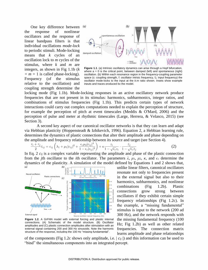
One key difference between

the response of nonlinear

oscillators and the response of

linear bandpass filters is that

individual oscillations mode-lock

to periodic stimuli. Mode-locking

means that k cycles of an

oscillation lock to m cycles of the

stimulus, where k and m are

integers, as shown in Fig 1.1b (k

= m = 1 is called phase-locking).

Frequency (of the stimulus

relative to the oscillation) and

coupling strength determine the

locking mode (Fig 1.1b). Mode-locking responses in an active oscillatory network produce

frequencies that are not present in its stimulus: harmonics, subharmonics, integer ratios, and

combinations of stimulus frequencies (Fig 1.1b). This predicts certain types of network

interactions could carry out complex computations needed to explain the perception of structure,

for example the perception of pitch at event timescales (Meddis & O'Mard, 2006) and the

perception of pulse and meter at rhythmic timescales (Large, Herrera, & Velasco, 2015) (see

Section 3).

A second key aspect of our canonical oscillator networks is that they can learn and adapt

via Hebbian plasticity (Hoppensteadt & Izhikevich, 1996). Equation 2, a Hebbian learning rule,

determines the dynamics of plastic connections that alter their amplitude and phase depending on

the amplitude and frequency relationship between its source and target (see Section 4).

(2)

In Eq. 2 cij is a complex variable representing the amplitude and phase of the plastic connection

from the jth oscillator to the ith oscillator. The parameters λ, μ1, μ2, κ, and ϵc determine the

dynamics of the plasticity. A simulation of the model defined by Equations 1 and 2 shows that,

unlike linear filters, canonical oscillators

resonate not only to frequencies present

in the external signal but also to their

harmonics, subharmonics, and nonlinear

combinations (Fig 1.2b). Plastic

connections grow strong between

oscillators if they exhibit certain simple

frequency relationships (Fig 1.2c). In

the example, a “missing fundamental”

stimulus is input to the network (200 ad

300 Hz), and the network responds with

the missing fundamental frequency (100

Hz; Fig 1.2b) as well as other related

frequencies. The connection matrix

learns amplitude and phase relationships

of the components (Fig 1.2c shows only amplitude, i.e. | cij |) and this information can be used to

“bind” the simultaneous components into an integrated percept.

Figure 1.1. (a) Intrinsic oscillatory dynamics can arise through a Hopf bifurcation, where a = 0 is the critical point, between damped (left) and spontaneous (right) oscillation. (b) Within each resonance region in the frequency-coupling parameter space (c: coupling strength, f: oscillator intrisic frequency, f0: input frequency) the oscillator mode-locks to the input at the k:m ratio shown. Insets show example inputs and traces produced by the model.

Figure 1.2. A GrFNN model with external forcing and plastic internal connections. (A) Schematic of the model structure. (B) Oscillator amplitudes and (C) plastic connection amplitudes after stimulation with an external signal containing 200 and 300 Hz sinusoids. Note the harmonic structure of the response, including the 100 Hz “missing fundamental”.


Summary: The model described by Equations 1 and 2 is a generic population-level model

(Hoppensteadt & Izhikevich, 1997) that captures the fundamental dynamics observed in neuron-

level models (Brunel, 2000; Stefanescu & Jirsa, 2008), but is amenable to theoretical and

computational analysis (Aronson, Ermentrout, & Kopell, 1990). The model is invariant over

temporal and spatial scale, and in Section 5 we use it to model active cochlear resonance to

sound (Lerud, Kim, Almonte, Carney, & Large, under revision), brainstem phase-locking to

pitch combinations (Lerud, Almonte, Kim, & Large, 2014), and cortical entrainment to rhythmic

patterns (e.g., Large et al., 2015). First, however, we describe the theoretical analyses that have

enabled us to create such models.

2. Signal Processing by Neural Oscillators

Despite its simple mathematical form, the canonical model for gradient frequency neural

networks is still difficult to analyze in its entirety because its dynamics is determined by complex

interactions among multiple network components. Oscillators in the network are driven by

external forcing and at the same time receive input from other oscillators, and both types of

interaction may involve linear and/or nonlinear coupling which can evolve over time via a

generalized form of Hebbian plasticity (Large, 2011; Hoppensteadt and Izhikevich, 1996). Our

approach is to analyze individual components of the network separately and attempt to

understand its overall dynamics as a combination of its component dynamics. To begin, we

analyzed and categorized the driven behaviors of canonical oscillators under periodic forcing.

Consider the following differential equation describing an oscillator in the canonical

model (or simply, a canonical oscillator) driven by sinusoidal forcing of fixed frequency, ω0, and

amplitude, F:

(3)

where ω = 2πf is the radian natural frequency. To understand the response of a gradient

frequency network, we focus on how the driven state of an oscillator changes as a function of its

natural frequency.

The autonomous behavior of the oscillator (i.e., when F = 0) is readily seen when it is

brought to polar coordinates using z = reiφ. Then, the amplitude and phase dynamics are

described by

Depending on the values

of α, β1, and β2, the

autonomous amplitude

vector field (the first

equation above) can have

one of four distinct

topologies. When

decreases monotonically

as r increases, the origin

is the only fixed point

which is stable as the

arrow indicates (Fig 2.1A). An oscillator with this type of amplitude vector field decays to zero

Figure 2.1. Autonomous behavior of a canonical oscillator in different

parameter regimes. Amplitude vector field is shown for (A) a critical Hopf

regime, (B) a supercritical Hopf regime, (C) a supercritical double limit cycle

regime, and (D) a subcritical double limit cycle regime. Filled circles indicate

stable fixed points (attractors) and empty circles unstable fixed points (repellers).

Arrows indicate the direction of trajectories in the vector field.


while oscillating at its natural

frequency. A representative

parameter regime for this type

is the critical point of a

supercritical Hopf bifurcation

(α = 0, β1 < 0). (A subcritical

Hopf bifurcation occurs when

α = 0 and β1 > 0.) When

increases from the origin and

then decreases after a local

maximum, there is a stable

nonzero fixed point while the

origin is rendered unstable (Fig

2.1B). An oscillator of this type

shows spontaneous oscillation

at the amplitude of the stable

fixed point (unless the initial

condition is zero). The

supercritical branch of a


(α > 0, β1 < 0) is an example.

When there are three fixed points with two local extrema, two of the fixed points are stable,

indicating bistability between equilibrium at zero and spontaneous oscillation at a nonzero

amplitude (Fig 2.1C). As the local maximum in the vector field moves below the r axis by, say,

decreasing β1, the two nonzero fixed points collide and vanish (Fig 2.1D). This transition is

called a double limit cycle (hereafter, DLC) bifurcation since it involves two limit cycles (closed

orbits) in the (r,φ) plane, one stable and the other unstable. Thus, we call the regime shown in

Fig 2.1C (α < 0, β1 > 0, β2 < 0, local max > 0) supercritical DLC and the one shown in Fig 2.1D

(α < 0, β1 > 0, β2 < 0, local max < 0) subcritical DLC. The subcritical DLC regime has only one

stable fixed point at zero but is different from the critical Hopf regime (Fig 2.1A) in that it has a

local maximum in the vector field.

To examine how a canonical oscillator responds to external forcing, we bring Equation 3

to polar coordinates, again using z = reiφ, and express its dynamics in terms of the relative phase

ψ = φ − ω0t so that a stable fixed point in (r,ψ) indicates a phase-locked state:

(4)

where Ω = ω − ω0 is the frequency difference between the oscillator and the input. We evaluate

the stability of fixed point(s) for a range of forcing parameters Ω and F wide enough to

encompass all possible qualitatively different driven behaviors of the four regimes of intrinsic

parameters introduced above.

Figure 2.2. Driven behavior of a critical Hopf oscillator. (A) Steady-state

amplitude and relative phase as a function of frequency difference (α = 0,

β1 = −100, β2 = 0, F = 0.2), with vertical dashed lines indicating the

frequency differences used for panels B–E, (B) trajectories attracted to a

stable node in the (r,ψ) plane starting from a set of different initial

conditions (Ω/2π = 0.1), (C) trajectories attracted to a stable spiral (Ω/2π =

0.5), (D) relative phase plotted over time for a trajectory in panel B (phase

locking), and (E) relative phase plotted over time for a trajectory in panel

C (phase locking). Filled circles in panels B and C indicate stable fixed

points.


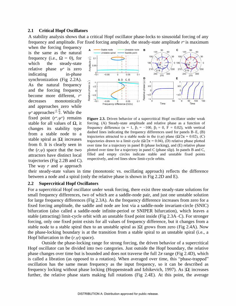
2.1 Critical Hopf Oscillators

A stability analysis shows that a critical Hopf oscillator phase-locks to sinusoidal forcing of any

frequency and amplitude. For fixed forcing amplitude, the steady-state amplitude r∗ is maximum

when the forcing frequency

is the same as the natural

frequency (i.e., Ω = 0), for

which the steady-state

relative phase ψ∗ is zero

indicating in-phase

synchronization (Fig 2.2A).

As the natural frequency

and the forcing frequency

become more different, r∗

decreases monotonically

and approaches zero while

ψ∗ approaches . While the

fixed point (r∗,ψ∗) remains

stable for all values of Ω, it

changes its stability type

from a stable node to a

stable spiral as |Ω| increases

from 0. It is clearly seen in

the (r,ψ) space that the two

attractors have distinct local

trajectories (Fig 2.2B and C).

The way r and ψ approach

their steady-state values in time (monotonic vs. oscillating approach) reflects the difference

between a node and a spiral (only the relative phase is shown in Fig 2.2D and E).

2.2 Supercritical Hopf Oscillators

For a supercritical Hopf oscillator under weak forcing, there exist three steady-state solutions for

small frequency differences, two of which are a saddle-node pair, and just one unstable solution

for large frequency differences (Fig 2.3A). As the frequency difference increases from zero for a

fixed forcing amplitude, the saddle and node are lost via a saddle-node invariant-circle (SNIC)

bifurcation (also called a saddle-node infinite-period or SNIPER bifurcation), which leaves a

stable (attracting) limit-cycle orbit with an unstable fixed point inside (Fig 2.3A–C). For stronger

forcing, only one fixed point exists for all values of frequency difference, but it changes from a

stable node to a stable spiral then to an unstable spiral as |Ω| grows from zero (Fig 2.4A). Now

the phase-locking boundary is at the transition from a stable spiral to an unstable spiral (i.e., a

Hopf bifurcation in the (r,ψ) space).

Outside the phase-locking range for strong forcing, the driven behavior of a supercritical

Hopf oscillator can be divided into two categories. Just outside the Hopf boundary, the relative

phase changes over time but is bounded and does not traverse the full 2π range (Fig 2.4D), which

is called a libration (as opposed to a rotation). When averaged over time, this “phase-trapped”

oscillation has the same mean frequency as the input frequency, so it can be described as

frequency locking without phase locking (Hoppensteadt and Izhikevich, 1997). As |Ω| increases

further, the relative phase starts making full rotations (Fig 2.4E). At this point, the average

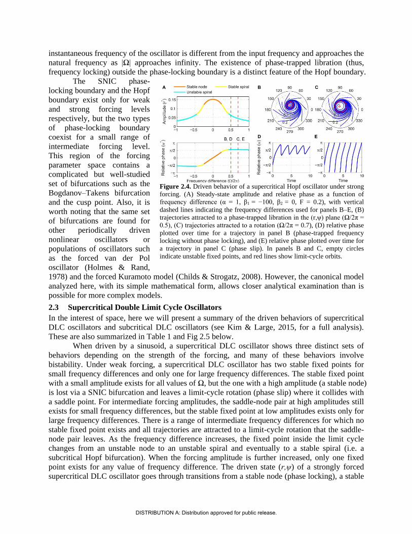
Figure 2.3. Driven behavior of a supercritical Hopf oscillator under weak

forcing. (A) Steady-state amplitude and relative phase as a function of

frequency difference (α = 1, β1 = −100, β2 = 0, F = 0.02), with vertical

dashed lines indicating the frequency differences used for panels B–E, (B)

trajectories attracted to a stable node in the (r,ψ) plane (Ω/2π = 0.02), (C)

trajectories drawn to a limit cycle (Ω/2π = 0.04), (D) relative phase plotted

over time for a trajectory in panel B (phase locking), and (E) relative phase

plotted over time for a trajectory in panel C (phase slip). In panels B and C,

filled and empty circles indicate stable and unstable fixed points

respectively, and red lines show limit-cycle orbits.


instantaneous frequency of the oscillator is different from the input frequency and approaches the

natural frequency as |Ω| approaches infinity. The existence of phase-trapped libration (thus,

frequency locking) outside the phase-locking boundary is a distinct feature of the Hopf boundary.

The SNIC phase-

locking boundary and the Hopf

boundary exist only for weak

and strong forcing levels

respectively, but the two types

of phase-locking boundary

coexist for a small range of

intermediate forcing level.

This region of the forcing

parameter space contains a

complicated but well-studied

set of bifurcations such as the

Bogdanov–Takens bifurcation

and the cusp point. Also, it is

worth noting that the same set

of bifurcations are found for

other periodically driven

nonlinear oscillators or

populations of oscillators such

as the forced van der Pol

oscillator (Holmes & Rand,

1978) and the forced Kuramoto model (Childs & Strogatz, 2008). However, the canonical model

analyzed here, with its simple mathematical form, allows closer analytical examination than is

possible for more complex models.

2.3 Supercritical Double Limit Cycle Oscillators

In the interest of space, here we will present a summary of the driven behaviors of supercritical

DLC oscillators and subcritical DLC oscillators (see Kim & Large, 2015, for a full analysis).

These are also summarized in Table 1 and Fig 2.5 below.

When driven by a sinusoid, a supercritical DLC oscillator shows three distinct sets of

behaviors depending on the strength of the forcing, and many of these behaviors involve

bistability. Under weak forcing, a supercritical DLC oscillator has two stable fixed points for

small frequency differences and only one for large frequency differences. The stable fixed point

with a small amplitude exists for all values of Ω, but the one with a high amplitude (a stable node)

is lost via a SNIC bifurcation and leaves a limit-cycle rotation (phase slip) where it collides with

a saddle point. For intermediate forcing amplitudes, the saddle-node pair at high amplitudes still

exists for small frequency differences, but the stable fixed point at low amplitudes exists only for

large frequency differences. There is a range of intermediate frequency differences for which no

stable fixed point exists and all trajectories are attracted to a limit-cycle rotation that the saddle-

node pair leaves. As the frequency difference increases, the fixed point inside the limit cycle

changes from an unstable node to an unstable spiral and eventually to a stable spiral (i.e. a

subcritical Hopf bifurcation). When the forcing amplitude is further increased, only one fixed

point exists for any value of frequency difference. The driven state (r,ψ) of a strongly forced

supercritical DLC oscillator goes through transitions from a stable node (phase locking), a stable

Figure 2.4. Driven behavior of a supercritical Hopf oscillator under strong

forcing. (A) Steady-state amplitude and relative phase as a function of

frequency difference (α = 1, β1 = −100, β2 = 0, F = 0.2), with vertical

dashed lines indicating the frequency differences used for panels B–E, (B)

trajectories attracted to a phase-trapped libration in the (r,ψ) plane (Ω/2π =

0.5), (C) trajectories attracted to a rotation (Ω/2π = 0.7), (D) relative phase

plotted over time for a trajectory in panel B (phase-trapped frequency

locking without phase locking), and (E) relative phase plotted over time for

a trajectory in panel C (phase slip). In panels B and C, empty circles

indicate unstable fixed points, and red lines show limit-cycle orbits.


spiral (phase locking), a libration around an unstable spiral (frequency locking without phase

locking), a rotation around an unstable spiral (phase slip), and lastly bistability between phase

locking on a stable spiral and phase slip on a stable limit cycle. So, a strongly forced supercritical

DLC oscillator has two phase-locking boundaries, a supercritical Hopf bifurcation and a

subcritical Hopf bifurcation.

2.4 Subcritical Double Limit Cycle Oscillators

Like a critical Hopf oscillator, a subcritical DLC oscillator is attracted to an equilibrium at zero

when it is not driven. But the presence of a local maximum in the amplitude vector field makes

its driven dynamics more varied and interesting than that of a critical Hopf oscillator. Like a

supercritical DLC oscillator, a subcritical DLC oscillator exhibits three different sets of driven

behaviors depending on the

forcing amplitude.

For weak forcing, it

behaves like a critical Hopf

oscillator, with its driven state

attracted to a stable node when

|Ω| is small and to a stable spiral

when |Ω| is large. For

intermediate forcing amplitudes,

a pair of fixed points appears at

high amplitudes and they are lost

via a saddle-node bifurcation at a

certain frequency difference, but

this saddle-node bifurcation does

not leave a limit cycle like a

SNIC bifurcation. When driven

strongly, a subcritical DLC

oscillator has the same set of

fixed points as a supercritical

DLC oscillator—a stable node, a

stable spiral, an unstable spiral,

and a stable spiral as |Ω|

increases from zero. A


occurs at the first phase-locking

boundary, where a stable spiral

turns unstable and a stable limit

cycle grows around it. However,

the limit cycle does not grow into a rotation that encompasses the origin, which is the case for a

supercritical DLC oscillator. Instead, it shrinks back and turns into a stable spiral via another

supercritical Hopf bifurcation. In the absence of a SNIC or subcritical Hopf bifurcation, a

strongly driven subcritical DLC oscillator shows no bistability and, since the only non-locked

behavior is a libration, it either phase-locks or frequency-locks to the input for all values of Ω.

2.5 Classification of Parameter Regimes by Driven Behavior

We can classify all possible parameter settings for canonical oscillators into four regimes

with distinct driven behaviors (Table 1 and Fig 2.5). Oscillators with an autonomous amplitude

Figure 2.5. Stability regions for a canonical oscillator under sinusoidal

forcing. The stability of driven state (r∗,ψ∗) is shown as a function of

forcing amplitude and frequency difference for (A) a critical Hopf

oscillator (α = 0, β1 = −100, β2 = 0), (B) a supercritical Hopf oscillator (α

= 1, β1 = −100, β2 = 0), (C) a supercritical double limit cycle oscillator (α

= −1, β1 = 4, β2 = −1, ε = 1), and (D) a subcritical double limit cycle

oscillator (α = −1, β1 = 2.5, β2 = −1, ε = 1). The color indicates the

stability type of a stable fixed point if there is one (purple if there are

two). If there is no stable fixed point, the color indicates the stability of

an unstable fixed point. Dashed horizontal lines indicate the forcing

amplitudes used for Figs. 2.2–2.4.


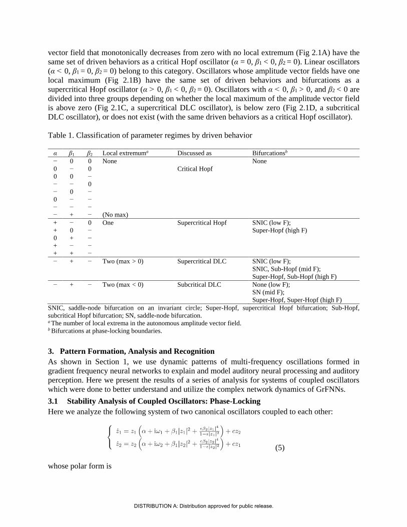
vector field that monotonically decreases from zero with no local extremum (Fig 2.1A) have the

same set of driven behaviors as a critical Hopf oscillator (α = 0, β1 < 0, β2 = 0). Linear oscillators

(α < 0, β1 = 0, β2 = 0) belong to this category. Oscillators whose amplitude vector fields have one

local maximum (Fig 2.1B) have the same set of driven behaviors and bifurcations as a

supercritical Hopf oscillator (α > 0, β1 < 0, β2 = 0). Oscillators with α < 0, β1 > 0, and β2 < 0 are

divided into three groups depending on whether the local maximum of the amplitude vector field

is above zero (Fig 2.1C, a supercritical DLC oscillator), is below zero (Fig 2.1D, a subcritical

DLC oscillator), or does not exist (with the same driven behaviors as a critical Hopf oscillator).

Table 1. Classification of parameter regimes by driven behavior

α β1 β2 Local extremuma Discussed as Bifurcationsb

− 0 0 None None

0 − 0 Critical Hopf

0 0 −

− − 0

− 0 −

0 − −

− − −

− + − (No max)

+ − 0 One Supercritical Hopf SNIC (low F);

+ 0 − Super-Hopf (high F)

0 + −

+ − −

+ + −

− + − Two (max > 0) Supercritical DLC SNIC (low F);

SNIC, Sub-Hopf (mid F);

Super-Hopf, Sub-Hopf (high F)

− + − Two (max < 0) Subcritical DLC None (low F);

SN (mid F);

Super-Hopf, Super-Hopf (high F)

SNIC, saddle-node bifurcation on an invariant circle; Super-Hopf, supercritical Hopf bifurcation; Sub-Hopf,

subcritical Hopf bifurcation; SN, saddle-node bifurcation. a The number of local extrema in the autonomous amplitude vector field. b Bifurcations at phase-locking boundaries.

3. Pattern Formation, Analysis and Recognition

As shown in Section 1, we use dynamic patterns of multi-frequency oscillations formed in

gradient frequency neural networks to explain and model auditory neural processing and auditory

perception. Here we present the results of a series of analysis for systems of coupled oscillators

which were done to better understand and utilize the complex network dynamics of GrFNNs.

3.1 Stability Analysis of Coupled Oscillators: Phase-Locking

Here we analyze the following system of two canonical oscillators coupled to each other:

(5)

whose polar form is


(6)

where zi = rieiφi,ψ = φ1 − φ2 and Ω = ω1 − ω2. We present the analysis of two coupled oscillators

for each parameter regime identified in Section 2.

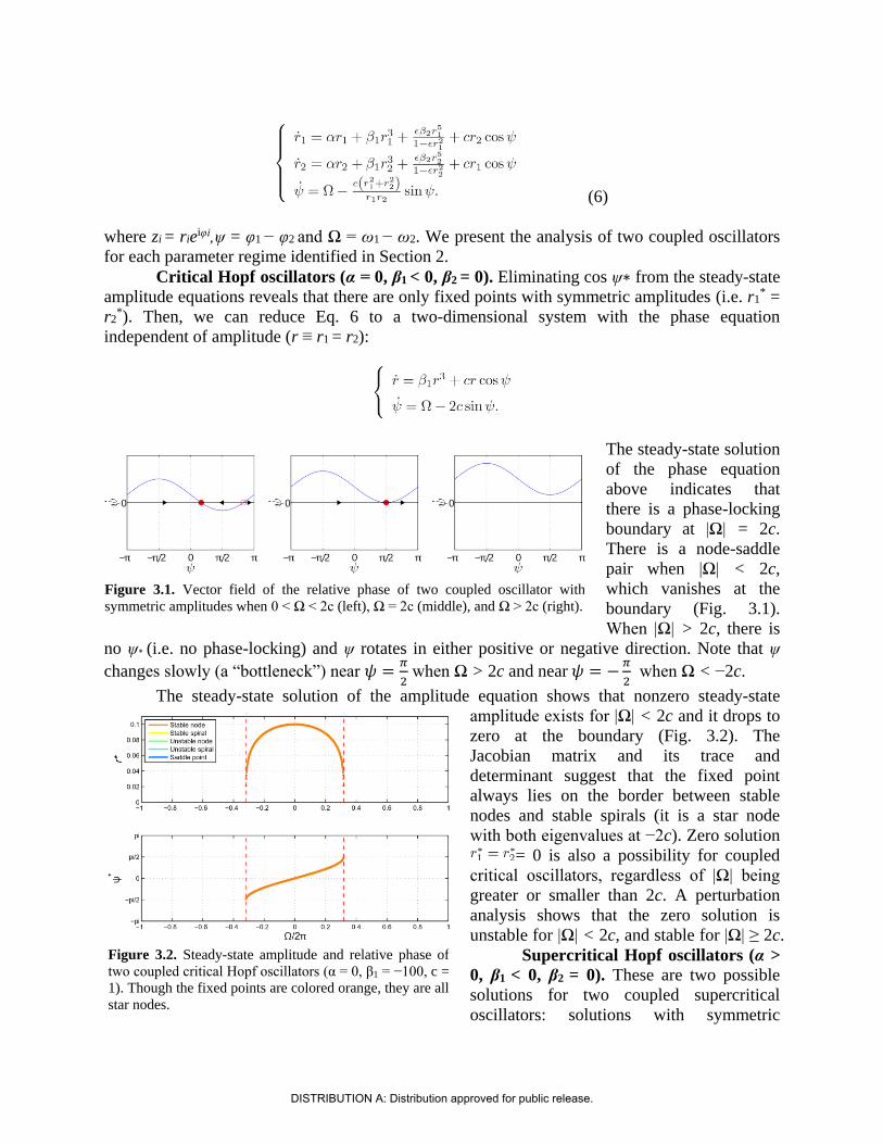
Critical Hopf oscillators (α = 0, β1 < 0, β2 = 0). Eliminating cos ψ∗ from the steady-state

amplitude equations reveals that there are only fixed points with symmetric amplitudes (i.e. r1* =

r2*). Then, we can reduce Eq. 6 to a two-dimensional system with the phase equation

independent of amplitude (r ≡ r1 = r2):

The steady-state solution

of the phase equation

above indicates that

there is a phase-locking

boundary at |Ω| = 2c.

There is a node-saddle

pair when |Ω| < 2c,

which vanishes at the

boundary (Fig. 3.1).

When |Ω| > 2c, there is

no ψ∗ (i.e. no phase-locking) and ψ rotates in either positive or negative direction. Note that ψ

changes slowly (a “bottleneck”) near 𝜓 =𝜋

2 when Ω > 2c and near 𝜓 = −

𝜋

2 when Ω < −2c.

The steady-state solution of the amplitude equation shows that nonzero steady-state

amplitude exists for |Ω| < 2c and it drops to

zero at the boundary (Fig. 3.2). The

Jacobian matrix and its trace and

determinant suggest that the fixed point

always lies on the border between stable

nodes and stable spirals (it is a star node

with both eigenvalues at −2c). Zero solution

= 0 is also a possibility for coupled

critical oscillators, regardless of |Ω| being

greater or smaller than 2c. A perturbation

analysis shows that the zero solution is

unstable for |Ω| < 2c, and stable for |Ω| ≥ 2c.

Supercritical Hopf oscillators (α >

0, β1 < 0, β2 = 0). These are two possible

solutions for two coupled supercritical

oscillators: solutions with symmetric

Figure 3.1. Vector field of the relative phase of two coupled oscillator with

symmetric amplitudes when 0 < Ω < 2c (left), Ω = 2c (middle), and Ω > 2c (right).

Figure 3.2. Steady-state amplitude and relative phase of

two coupled critical Hopf oscillators (α = 0, β1 = −100, c =

1). Though the fixed points are colored orange, they are all

star nodes.


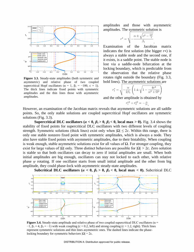
amplitudes and those with asymmetric

amplitudes. The symmetric solution is

.

Examination of the Jacobian matrix

indicates the first solution (the bigger r∗) is

always a stable node and the second one, if

it exists, is a saddle point. The stable node is

lost via a saddle-node bifurcation at the

locking boundary, which is predictable from

the observation that the relative phase

rotates right outside the boundary (Fig. 3.3,

bold lines). The asymmetric solutions are

and the other amplitude is obtained by

.

However, an examination of the Jacobian matrix reveals that asymmetric solutions are all saddle

points. So, the only stable solutions are coupled supercritical Hopf oscillators are symmetric

solutions (Fig. 3.3).

Supercritical DLC oscillators (α < 0, β1 > 0, β2 < 0, local max > 0). Fig. 3.4 shows the

stability of fixed points for supercritical DLC oscillators with two different levels of coupling

strength. Symmetric solutions (thick lines) exist only when |Ω| ≤ 2c. Within this range, there is

only one stable nonzero fixed point with symmetric amplitudes, which is always a node. They

also have stable fixed points with asymmetric amplitudes, due to their bistability. When coupling

is weak enough, stable asymmetric solutions exist for all values of Ω. For stronger coupling, they

exist for large values of |Ω| only. Three distinct behaviors are possible for |Ω| > 2c. Zero solution

is stable so that both oscillators can decay to zero if initial amplitudes are small. When both

initial amplitudes are big enough, oscillators can stay not locked to each other, with relative

phase ψ rotating. If one oscillator starts from small initial amplitude and the other from big

amplitude, they could phase-lock with asymmetric steady-state amplitudes.

Subcritical DLC oscillators (α < 0, β1 > 0, β2 < 0, local max < 0). Subcritical DLC

Figure 3.3. Steady-state amplitudes (both symmetric and

asymmetric) and relative phase of two coupled

supercritical Hopf oscillators (α = 1, β1 = −100, c = 1).

The thick lines indicate fixed points with symmetric

amplitudes and the thin lines those with asymmetric

amplitudes.

Figure 3.4. Steady-state amplitude and relative phase of two coupled supercritical DLC oscillators (α =

−1, β1 = 4, β2 = −1) with weak coupling (c = 0.2, left) and strong coupling (c = 1.2, right). Thick lines

represent symmetric solutions and thin lines asymmetric ones. The dashed lines indicate the phase-

locking boundary for symmetric behaviors |Ω| = 2c.


oscillators have nonzero symmetric r*’s for a subset of |Ω| ≤ 2c. When coupling is weak and

satisfies the following condition, there is no nonzero r* for all values of Ω and zero solution is the

only stable fixed point:

.

This is when the local maximum in amplitude vector field is below zero even for Ω = 0. With

stronger coupling, nonzero symmetric r*’s exist for the following range of Ω, which is a subset

of |Ω| ≤ 2c:

.

As shown in Fig. 3.5, fixed points with asymmetric amplitudes exist for coupled subcritical DLC

oscillators. Most of them are unstable saddle points, but with strong coupling there is a narrow

range of |Ω| just outside |Ω| = 2c where stable spirals exist.

3.2 Stability Analysis of Coupled Oscillators: Mode-Locking

When two oscillators have natural frequencies whose ratio is close to an integer ratio, they can

mode-lock to each other via resonant monomials. Two canonical oscillators mode-locking to

each other can be described by

,

for which we assume β2 < 0 in order to make the system stable given arbitrarily high k and m.

We bring the system to polar coordinates using zi = rieiφi and define ψ = mφ1 − kφ2 and Ω = mω1 −

kω2 to get

Assuming symmetric solutions, the system can be a two-dimensional system of r (≡ r1 = r2)

and ψ, for which the steady-state solutions can be obtained by solving

Figure 3.5. Steady-state amplitude and relative phase of two coupled subcritical DLC oscillators (α = −1,

β1 = 2.5, β2 = −1) with weak coupling (c = 0.3, left) and strong coupling (c = 1.2, right).


.

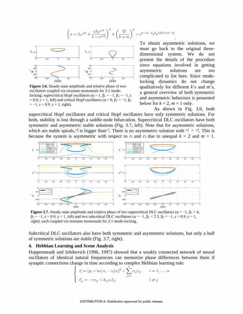
To obtain asymmetric solutions, we

must go back to the original three-

dimensional system. We do not

present the details of the procedure

since equations involved in getting

asymmetric solutions are too

complicated to list here. Since mode-

locking dynamics do not change

qualitatively for different k’s and m’s,

a general overview of both symmetric

and asymmetric behaviors is presented

below for k = 2, m = 1 only.

As shown in Fig. 3.6, both

supercritical Hopf oscillators and critical Hopf oscillators have only symmetric solutions. For

both, stability is lost through a saddle-node bifurcation. Supercritical DLC oscillators have both

symmetric and asymmetric stable solutions (Fig. 3.7, left). Note that for asymmetric solutions,

which are stable spirals, is bigger than . There is no asymmetric solution with . This is

because the system is asymmetric with respect to r1 and r2 due to unequal k = 2 and m = 1.

Subcritical DLC oscillators also have both symmetric and asymmetric solutions, but only a half

of symmetric solutions are stable (Fig. 3.7, right).

4. Hebbian Learning and Scene Analysis

Hoppensteadt and Izhikevich (1996, 1997) showed that a weakly connected network of neural

oscillators of identical natural frequencies can memorize phase differences between them if

synaptic connections change in time according to complex Hebbian learning rule:

Figure 3.6. Steady-state amplitude and relative phase of two

oscillators coupled via resonant monomials for 2:1 mode-

locking: supercritical Hopf oscillators (α = 1, β1 = −1, β2 = −1, ε

= 0.9, c = 1, left) and critical Hopf oscillators (α = 0, β1 = −1, β2

= −1, ε = 0.9, c = 1, right).

Figure 3.7. Steady-state amplitude and relative phase of two supercritical DLC oscillators (α = −1, β1 = 4,

β2 = −1, ε = 0.9, c = 1, left) and two subcritical DLC oscillators (α = −1, β1 = 2.5, β2 = −1, ε = 0.9, c = 1,

right), each coupled via resonant monomials for 2:1 mode-locking.


where ′ = d/dτ, τ = εt is ‘slow’ time, and γ and kij are positive real numbers. Note that the learning

rule has only a linear intrinsic term and an input term. When zi and zj oscillate at the same

frequency, the input term 𝑘𝑖𝑗𝑧𝑖𝑧 becomes a complex constant whose phase is the phase

difference between zi and zj. So, the phase of cij eventually comes to match the phase difference

between the oscillators it connects.

We expanded Hoppensteadt and Izhikevich’s single-frequency network with linear

learning rule into a multi-frequency network with nonlinear learning rule. We show that this

expansion gives rise to a set of rich dynamics that are not observed in either single-frequency

systems or systems without plasticity. Here, we analyze the dynamics of two simplest oscillator

systems with plastic connections: an oscillator with plastic coupling to single external input and

two oscillators connected by plastic coupling.

4.1 Plastic Coupling to External Forcing

Consider a single oscillator z that is driven by external forcing x via plastic coupling c.

Introducing fully expanded intrinsic terms to both the oscillator equation and the learning rule

gives us the following system:

where κ is a positive real number representing learning rate.

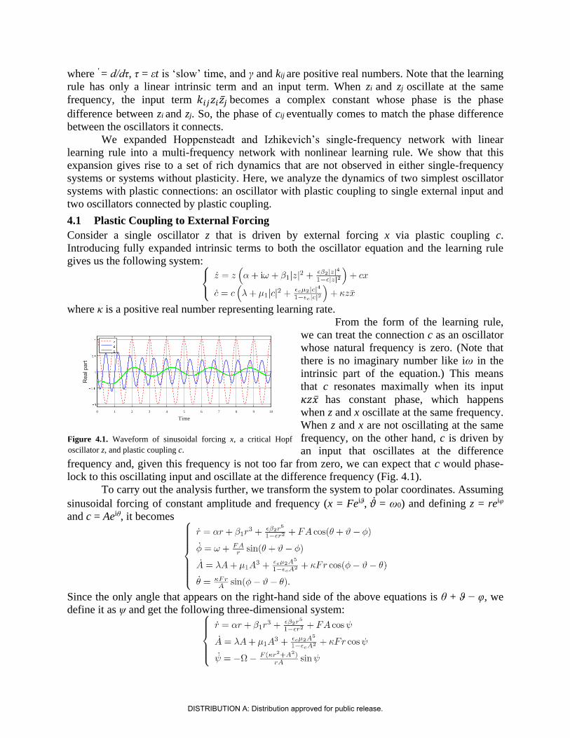
From the form of the learning rule,

we can treat the connection c as an oscillator

whose natural frequency is zero. (Note that

there is no imaginary number like iω in the

intrinsic part of the equation.) This means

that c resonates maximally when its input

𝜅𝑧 has constant phase, which happens

when z and x oscillate at the same frequency.

When z and x are not oscillating at the same

frequency, on the other hand, c is driven by

an input that oscillates at the difference

frequency and, given this frequency is not too far from zero, we can expect that c would phase-

lock to this oscillating input and oscillate at the difference frequency (Fig. 4.1).

To carry out the analysis further, we transform the system to polar coordinates. Assuming

sinusoidal forcing of constant amplitude and frequency (x = Feiϑ, = ω0) and defining z = reiφ

and c = Aeiθ, it becomes

Since the only angle that appears on the right-hand side of the above equations is θ + ϑ − φ, we

define it as ψ and get the following three-dimensional system:

0 1 2 3 4 5 6 7 8 9 10

Time

Figure 4.1. Waveform of sinusoidal forcing x, a critical Hopf

oscillator z, and plastic coupling c.


where Ω = ω − ω0. Since the fully expanded system is difficult, if not impossible, to solve, let us

examine the following truncated version (i.e. we assume β2 = µ2 = 0):

Now that both the oscillator and the learning rule have multiple parameter regimes with

distinct behaviors, we are going to briefly describe each combination of the regimes for oscillator

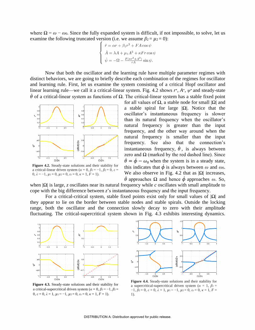
and learning rule. First, let us examine the system consisting of a critical Hopf oscillator and

linear learning rule—we call it a critical-linear system. Fig. 4.2 shows r∗, A∗, ψ∗ and steady-state

of a critical-linear system as functions of Ω. The critical-linear system has a stable fixed point

for all values of Ω, a stable node for small |Ω| and

a stable spiral for large |Ω|. Notice that the

oscillator’s instantaneous frequency is slower

than its natural frequency when the oscillator’s

natural frequency is greater than the input

frequency, and the other way around when the

natural frequency is smaller than the input

frequency. See also that the connection’s

instantaneous frequency, , is always between

zero and Ω (marked by the red dashed line). Since

= − 𝜔0 when the system is in a steady state,

this indicates that is always between ω and ω0.

We also observe in Fig. 4.2 that as |Ω| increases,

approaches Ω and hence approaches ω. So,

when |Ω| is large, z oscillates near its natural frequency while c oscillates with small amplitude to

cope with the big difference between z’s instantaneous frequency and the input frequency.

For a critical-critical system, stable fixed points exist only for small values of |Ω| and

they appear to lie on the border between stable nodes and stable spirals. Outside the locking

range, both the oscillator and the connection slowly decay to zero with their amplitude

fluctuating. The critical-supercritical system shown in Fig. 4.3 exhibits interesting dynamics.

Figure 4.2. Steady-state solutions and their stability for

a critical-linear driven system (α = 0, β1 = −1, β2 = 0, ε =

0, λ = −1, µ1 = 0, µ2 = 0, εc = 0, κ = 1, F = 1).


a critical-supercritical driven system (α = 0, β1 = −1, β2 =

0, ε = 0, λ = 1, µ1 = −1, µ2 = 0, εc = 0, κ = 1, F = 1).


a supercritical-supercritical driven system (α = 1, β1 =

−1, β2 = 0, ε = 0, λ = 1, µ1 = −1, µ2 = 0, εc = 0, κ = 1, F =

1).


Contrary to the critical-linear system shown earlier, converges to zero (thus approaches ω0)

as |Ω| increases toward infinity. This is because the connection has nonzero spontaneous

amplitude so that its amplitude cannot be lowered indefinitely. The supercritical-linear and

supercritical-critical systems have similar overall dynamics to the critical-linear system, except

that the oscillators’ amplitude converges to their nonzero spontaneous amplitude as |Ω| increases.

The supercritical-supercritical system shown in Fig. 4.4 has stable fixed points for only small |Ω|

and the locking boundary is a saddle-node bifurcation point. Outside the locking range, both the

oscillator and the connection fluctuate near their spontaneous amplitudes and intrinsic

frequencies.

4.2 Two Oscillators with Plastic Coupling

The dynamics of two canonical oscillators connected through plastic coupling can be described

by

Defining zi = rieiφi and cij = Aijeiθij, the above system is transformed to

Note that there are only two distinct arguments for trigonometric functions on the right-hand side

of the equations above. Defining them as ψ12 = θ12−φ1+φ2 and ψ21 = θ21 − φ2 + φ1 turns the above

eight-dimensional system into a six-dimensional one:

where Ω = ω1 − ω2.

From the definition of ψ12 and ψ21, we can see that 12 = 1 − 2 and 21 = 2 − 1

when the system is in a steady state (i.e. 12 = 21 = 0). In other words, the connections

oscillate at the instantaneous frequency difference of the oscillators they connect. This also

means that when two oscillators have different instantaneous frequencies, two connections


should have instantaneous frequencies of the same

magnitude but in opposite directions (i.e. 12 =

−21 ). Another property that can be expected

from the definition of ψ12 and ψ21 is that steady-

state θ12, θ21 and φ1 −φ2 should be neutrally stable

when Ω = 0, as was observed for driven oscillators

with plastic coupling to input.

We can reduce the dimension of the

system further by assuming that two oscillators

and two connections show symmetric behaviors.

This is a valid as well as useful assumption, since

stable fixed points are always symmetric for many

parameter regimes. However, it does not capture

any of asymmetric behaviors that can be stable

attractors for supercritical DLC oscillators. Using the substitutions r ≡ r1 = r2, A ≡ A12 = A21 and ψ

≡ ψ12 = −ψ21, we get the following three-dimensional system:

As we did above for oscillators with plastic coupling to external forcing, we will briefly

examine different possible combinations of the regimes for oscillator and learning rule. The

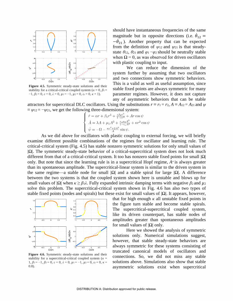
critical-critical system (Fig. 4.5) has stable nonzero symmetric solutions for only small values of

|Ω|. The symmetric steady-state behavior of a critical-supercritical system does not look much

different from that of a critical-critical system. It too has nonzero stable fixed points for small |Ω|

only. But note that since the learning rule is in a supercritical Hopf regime, A∗ is always greater

than its spontaneous amplitude. The supercritical-linear system is similar to the driven system in

the same regime—a stable node for small |Ω| and a stable spiral for large |Ω|. A difference

between the two systems is that the coupled system shown here is unstable and blows up for

small values of |Ω| when κ ≥ β1λ. Fully expanded intrinsic damping terms with negative β2 and µ2

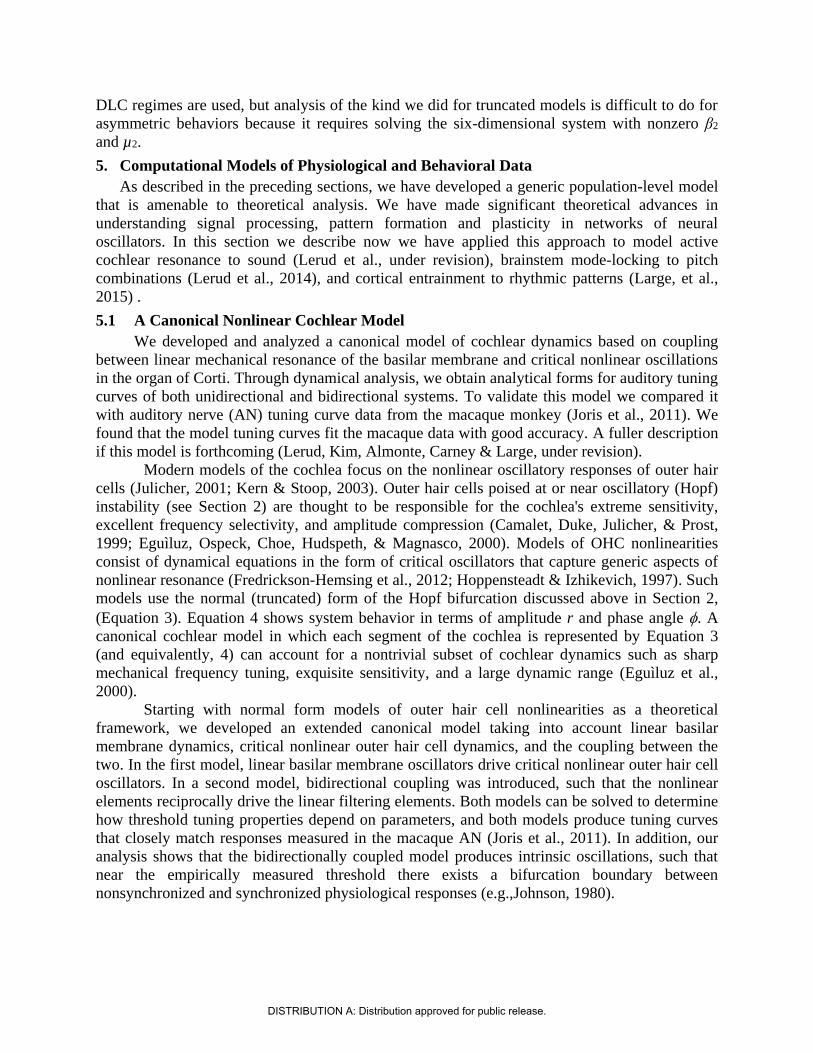
solve this problem. The supercritical-critical system shown in Fig. 4.6 has also two types of

stable fixed points (nodes and spirals) but these exist for small values of |Ω|. It appears, however,

that for high enough κ all unstable fixed points in

the figure turn stable and become stable spirals.

The supercritical-supercritical coupled system,

like its driven counterpart, has stable nodes of

amplitudes greater than spontaneous amplitudes

for small values of |Ω| only.

Here we showed the analysis of symmetric

solutions only. Numerical simulations suggest,

however, that stable steady-state behaviors are

always symmetric for these systems consisting of

truncated canonical models of oscillators and

connections. So, we did not miss any stable

solutions above. Simulations also show that stable

asymmetric solutions exist when supercritical

Figure 4.5. Symmetric steady-state solutions and their

stability for a critical-critical coupled system (α = 0, β1 =

−1, β2 = 0, ε = 0, λ = 0, µ1 = −1, µ2 = 0, εc = 0, κ = 1).

Figure 4.6. Symmetric steady-state solutions and their

stability for a supercritical-critical coupled system (α =

1, β1 = −1, β2 = 0, ε = 0, λ = 0, µ1 = −1, µ2 = 0, εc = 0, κ =

0.8).


DLC regimes are used, but analysis of the kind we did for truncated models is difficult to do for

asymmetric behaviors because it requires solving the six-dimensional system with nonzero β2

and µ2.

5. Computational Models of Physiological and Behavioral Data

As described in the preceding sections, we have developed a generic population-level model

that is amenable to theoretical analysis. We have made significant theoretical advances in

understanding signal processing, pattern formation and plasticity in networks of neural

oscillators. In this section we describe now we have applied this approach to model active

cochlear resonance to sound (Lerud et al., under revision), brainstem mode-locking to pitch

combinations (Lerud et al., 2014), and cortical entrainment to rhythmic patterns (Large, et al.,

2015) .

5.1 A Canonical Nonlinear Cochlear Model

We developed and analyzed a canonical model of cochlear dynamics based on coupling

between linear mechanical resonance of the basilar membrane and critical nonlinear oscillations

in the organ of Corti. Through dynamical analysis, we obtain analytical forms for auditory tuning

curves of both unidirectional and bidirectional systems. To validate this model we compared it

with auditory nerve (AN) tuning curve data from the macaque monkey (Joris et al., 2011). We

found that the model tuning curves fit the macaque data with good accuracy. A fuller description

if this model is forthcoming (Lerud, Kim, Almonte, Carney & Large, under revision).

Modern models of the cochlea focus on the nonlinear oscillatory responses of outer hair

cells (Julicher, 2001; Kern & Stoop, 2003). Outer hair cells poised at or near oscillatory (Hopf)

instability (see Section 2) are thought to be responsible for the cochlea's extreme sensitivity,

excellent frequency selectivity, and amplitude compression (Camalet, Duke, Julicher, & Prost,

1999; Eguìluz, Ospeck, Choe, Hudspeth, & Magnasco, 2000). Models of OHC nonlinearities

consist of dynamical equations in the form of critical oscillators that capture generic aspects of

nonlinear resonance (Fredrickson-Hemsing et al., 2012; Hoppensteadt & Izhikevich, 1997). Such

models use the normal (truncated) form of the Hopf bifurcation discussed above in Section 2,

(Equation 3). Equation 4 shows system behavior in terms of amplitude r and phase angle . A

canonical cochlear model in which each segment of the cochlea is represented by Equation 3

(and equivalently, 4) can account for a nontrivial subset of cochlear dynamics such as sharp

mechanical frequency tuning, exquisite sensitivity, and a large dynamic range (Eguìluz et al.,

2000).

Starting with normal form models of outer hair cell nonlinearities as a theoretical

framework, we developed an extended canonical model taking into account linear basilar

membrane dynamics, critical nonlinear outer hair cell dynamics, and the coupling between the

two. In the first model, linear basilar membrane oscillators drive critical nonlinear outer hair cell

oscillators. In a second model, bidirectional coupling was introduced, such that the nonlinear

elements reciprocally drive the linear filtering elements. Both models can be solved to determine

how threshold tuning properties depend on parameters, and both models produce tuning curves

that closely match responses measured in the macaque AN (Joris et al., 2011). In addition, our

analysis shows that the bidirectionally coupled model produces intrinsic oscillations, such that

near the empirically measured threshold there exists a bifurcation boundary between

nonsynchronized and synchronized physiological responses (e.g.,Johnson, 1980).


5.1.1 Unidirectional Model

We used pairs of coupled oscillators to model the dynamics of cochlear segments. In each

pair, one oscillator represents BM displacement dynamics, and the other represents organ of

Corti (OC) dynamics, including the outer hair cells, the tectorial membrane, and other supporting

structures. Input to the complex drives the BM oscillator, which is intended to account for the

dynamical effects of the cochlear fluid traveling waves that drive the BM. The OC energy source

stems from critical oscillations that cause the organ of Corti to vibrate. Thus, the model exhibits

both BM filtering and critical oscillations that capture the amplification, compression, and

frequency selectivity of cochlear processing (Eguìluz et al., 2000).

The natural frequency of each BM-OC complex is set to correspond to the best frequency

of the cochlear segment that it represents. We equate the state of the OC oscillator with the signal

that is transmitted to the AN. These broad considerations lead to a coupled set of canonical

oscillator equations for modeling a BM-OC complex:

The state variable zBM represents the dynamics of the BM, while zOC represents the

dynamics of the OC, including the nonlinearities of the OHCs. For simplicity, we assume a linear

BM. This leads to bandpass filtering behavior, making the model conceptually similar to that of

(Julicher, Andor, & Duke, 2001). The linear damping parameter, < 0, is determined by

fitting tuning-curve data. For the OC we assume critical nonlinear oscillation, i.e., = 0,

resulting in optimal amplification. The nonlinear damping parameter < 0 provides amplitude

compression in the OC and is also determined by fitting tuning-curve data. Finally, the parameter

c21 governs the relative strength of forcing of the OC by the BM and is determined by fitting the

data as well.

Because the model is described in terms of the complex state variables zBM and zOC, it can

be rewritten in polar form, giving rise to amplitude and phase equations:

Given the threshold amplitude r*

OC, which is a small number that we hold constant across tuning

curves, the formula for F only in terms of model parameters is

F is normally in pascals which can then be converted to the stimulus level L in dB SPL by L=20

log (F/p0) - G, where p0 = 20Pa represents the reference pressure, and G the gain of the middle

ear filter in dB.


To determine tuning curves that can be compared with auditory-nerve data, we first pass

the acoustic stimulus through a linear filter to approximate the amplitude and phase response of

the middle ear (Bruce, Sachs, & Young, 2003; Zilany & Bruce, 2006). The middle-ear filter is a

simplified form of that of Bruce (2003). Zilany and Bruce developed a fifth-order continuous-

time transfer function and represented it as a fifth-order digital filter using a bilinear

transformation for a sampling frequency of 500 kHz, with the frequency axis pre-warped to give

a matching frequency response at 1 kHz. To ensure stability of the digital filter, it was

implemented in a second-order system form by cascading digital filters. Once the MEF and

cochlear BM-OC oscillatory complexes are defined, the resulting waveform is provided as input.

The three parameters, < 0, < 0, and c21 > 0, are determined using a search

procedure that adjusts model parameters to obtain a sufficiently close match to the data. We held

the threshold r*OC = 0.1 constant and fit each curve individually. The results of the parameter

searches are shown in green in Figure 5.1 A, B, and C, for low, mid, and high frequency tuning

curves from the Joris et al. data set, respectively. The average root-mean-square error for the fits

in was 6.9219 dB. It was noted that both and varied within a single order of magnitude

over all tuning curves, and c21 was a reliable linear function of CF.

5.1.2 Bidirectional Model

A more realistic configuration of the BM-OC oscillatory complexes is to use bidirectional

coupling between the two oscillators rather than unidirectional coupling used in the previous

model. Thus, our second model considers the effect of OC dynamics on the BM. With

bidirectional coupling, the dynamics of an oscillatory complex are governed by

with c12 being the coupling coefficient of the OC oscillator feeding back to the BM oscillator.

Similarly to the unidirectional model, we can get a closed-form formula for forcing amplitude F

expressed as a function of threshold amplitude r*OC, frequency difference , and model

parameters:

where

Stability analysis of this system reveals that bidirectional coupling introduces an important

change in the dynamics of BM-OC complexes. With unidirectional coupling and with set to

zero or below, both the BM and OC oscillators decay to zero when not driven by external forcing.

With bidirectional coupling, however, the two oscillators provide input to each other and as a


result they have nonzero steady-state amplitudes even in the absence of external forcing. A

consequence of having nonzero spontaneous amplitude is that a BM-OC complex with

bidirectional coupling may not phase-lock to external forcing if its natural frequency is too

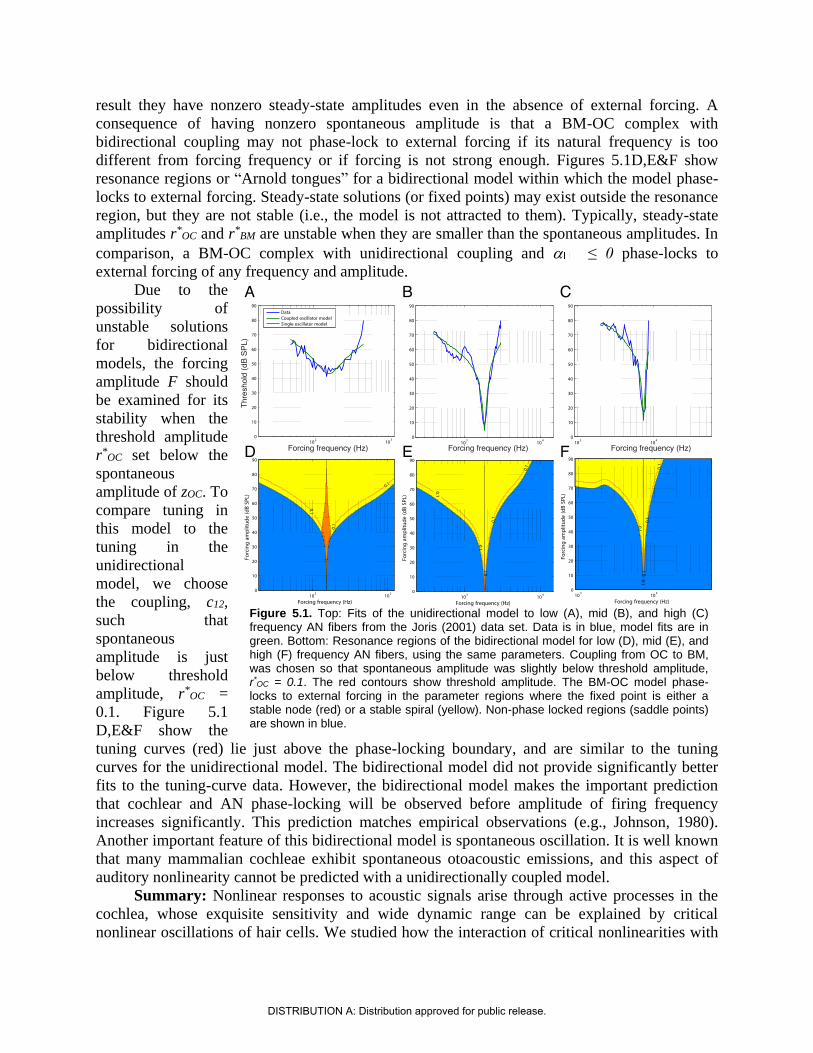
different from forcing frequency or if forcing is not strong enough. Figures 5.1D,E&F show

resonance regions or “Arnold tongues” for a bidirectional model within which the model phase-

locks to external forcing. Steady-state solutions (or fixed points) may exist outside the resonance

region, but they are not stable (i.e., the model is not attracted to them). Typically, steady-state

amplitudes r*OC and r*

BM are unstable when they are smaller than the spontaneous amplitudes. In

comparison, a BM-OC complex with unidirectional coupling and ≤ 0 phase-locks to

external forcing of any frequency and amplitude.

Due to the

possibility of

unstable solutions

for bidirectional

models, the forcing

amplitude F should

be examined for its

stability when the

threshold amplitude

r*OC set below the

spontaneous

amplitude of zOC. To

compare tuning in

this model to the

tuning in the

unidirectional

model, we choose

the coupling, c12,

such that

spontaneous

amplitude is just

below threshold

amplitude, r*OC =

0.1. Figure 5.1

D,E&F show the

tuning curves (red) lie just above the phase-locking boundary, and are similar to the tuning

curves for the unidirectional model. The bidirectional model did not provide significantly better

fits to the tuning-curve data. However, the bidirectional model makes the important prediction

that cochlear and AN phase-locking will be observed before amplitude of firing frequency

increases significantly. This prediction matches empirical observations (e.g., Johnson, 1980).

Another important feature of this bidirectional model is spontaneous oscillation. It is well known

that many mammalian cochleae exhibit spontaneous otoacoustic emissions, and this aspect of

auditory nonlinearity cannot be predicted with a unidirectionally coupled model.

Summary: Nonlinear responses to acoustic signals arise through active processes in the

cochlea, whose exquisite sensitivity and wide dynamic range can be explained by critical

nonlinear oscillations of hair cells. We studied how the interaction of critical nonlinearities with

Figure 5.1. Top: Fits of the unidirectional model to low (A), mid (B), and high (C) frequency AN fibers from the Joris (2001) data set. Data is in blue, model fits are in green. Bottom: Resonance regions of the bidirectional model for low (D), mid (E), and high (F) frequency AN fibers, using the same parameters. Coupling from OC to BM, was chosen so that spontaneous amplitude was slightly below threshold amplitude, r*

OC = 0.1. The red contours show threshold amplitude. The BM-OC model phase-locks to external forcing in the parameter regions where the fixed point is either a stable node (red) or a stable spiral (yellow). Non-phase locked regions (saddle points) are shown in blue.


the basilar membrane and other organ of Corti components could determine tuning properties of

the mammalian cochlea. We developed a canonical model in which the dynamics of the basilar

membrane–organ of Corti interaction is captured using pairs of coupled oscillators tuned to a

gradient of natural frequencies. We first developed a minimal model in which a linear oscillator,

representing basilar membrane dynamics, is coupled to a nonlinear oscillator poised at a Hopf

instability, which captures the nonlinear responses of outer hair cells and related organ of Corti

components. Parameters were determined by fitting the auditory-nerve tuning curves of macaque

monkeys. We then developed a more sophisticated model, taking into account bidirectional

coupling. We found that the unidirectionally and bidirectionally coupled models account equally

well for threshold tuning, but the bidirectionally coupled model also exhibited low amplitude,

spontaneous oscillation, providing a model that phase-locks to sound.

5.2 Brainstem Processing of Pitch Combinations

While some nonlinear responses arise through active processes in the cochlea, others arise

in neural populations of the cochlear nucleus, inferior colliculus and higher auditory areas.

Recently mode-locking, a generalization of phase locking that implies an intrinsically nonlinear

processing of sound, has been observed in mammalian auditory brainstem nuclei. We developed

a canonical model of mode-locked neural oscillation in brainstem that predicts the complex

nonlinear population responses to musical intervals that have been observed in the human

brainstem (for complete details, see Lerud et al., 2014).

In central auditory circuits, action potentials phase-lock to both the fine time structure

and the temporal envelope modulations of auditory stimuli at many different levels, including

cochlear nucleus, superior olive, inferior colliculus, thalamus, and A1 (Langner, 1992).

Traditionally, phase-locked spiking in the central auditory system is thought to represent an

essentially passive transmission of synchronized basilar membrane motion. An alternative

possibility is that active circuits in the central auditory system carry synchronized neural activity

forward. If this is the case, nonlinearities observed at the level of the brainstem might also arise

due to mode-locking (see Section 3), a phenomenon that has been observed in the auditory

brainstem (Langner, 1992), and is physiologically distinct from the mechanical compression and

half-wave rectification that occurs in the organ of Corti.

Mode-locking to acoustic signals has been observed in guinea pig cochlear nucleus

chopper and onset neurons (Laudanski et al., 2010), and mode- locking to the difference tone of

two dichotically presented stimulus frequencies has been observed in vivo and isolated to the

inferior colliculus of the chinchilla (Arnold and Burkard, 1998, 2000). Mode-locked spiking

patterns are often observed in vitro under DC injection (Brumberg and Gutkin, 2007), and active

oscillations have been observed in vivo in the inferior colliculus of the chicken (Schwarz et al.,

1993). Such observations lead to the possibility that the nonlinear responses observed in the

human auditory brainstem might arise, in part, due to mode-locking neurodynamics.

We modeled nonlinear responses to musical intervals that have been measured in the

human auditory brainstem response (Lee et al., 2009, see Fig. 2). In that study, the brainstem

representation of the musical intervals comprised not only stimulus frequencies, but also

numerous resonances at frequencies that were not physically present in the stimulus. How did

these frequencies arise? The stimuli were the intervals major sixth (G and E, “consonant”) and

minor seventh (F# and E, “dissonant”) which have fundamental frequency ratios of 1.6 (166

Hz/99 Hz) and 1.7 (166 Hz/93 Hz), making it unlikely that interaction of the fundamental

frequencies created strong distortion products in the cochlea (Dhar et al., 2009, 2005; Knight and

Kemp, 2001). Moreover, the responses of trained musicians were significantly enhanced


compared with those of novice listeners, implying experience- based differences that would not

have arisen at the level of the cochlea or auditory nerve (e.g., Large, Kozloski, & Crawford, 1998;

Laudanski et al., 2010).

The stimuli from the Lee et al. (2009) study were used as input to a cochlear model (see

Section 5.1), which in turn provided input to two brainstem network layers. The characteristic

frequencies of the cochlear layer and both brainstem layers spanned four octaves with 99

oscillators per octave. Thus, each layer included 397 oscillators, with characteristic frequencies

ranging from 64 Hz to 1024 Hz, encompassing the range of frequencies for which time-locked

responses have been observed in midbrain physiology (Langner, 1992). The cochlear model

includes a middle ear filter and simulates the basilar membrane and the organ of Corti (cf.

Jülicher et al., 2001 B). The cochlea is connected to the first brainstem layer, representing the

cochlear nucleus (CN), and the CN is connected to the second brainstem layer, representing the

inferior colliculus/ lateral lemniscus (IC/LL).

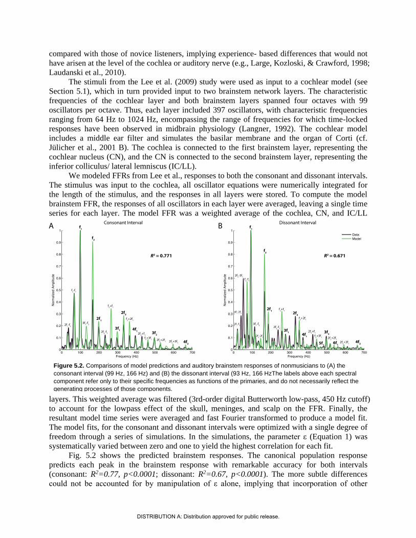
We modeled FFRs from Lee et al., responses to both the consonant and dissonant intervals.

The stimulus was input to the cochlea, all oscillator equations were numerically integrated for

the length of the stimulus, and the responses in all layers were stored. To compute the model

brainstem FFR, the responses of all oscillators in each layer were averaged, leaving a single time

series for each layer. The model FFR was a weighted average of the cochlea, CN, and IC/LL

layers. This weighted average was filtered (3rd-order digital Butterworth low-pass, 450 Hz cutoff)

to account for the lowpass effect of the skull, meninges, and scalp on the FFR. Finally, the

resultant model time series were averaged and fast Fourier transformed to produce a model fit.

The model fits, for the consonant and dissonant intervals were optimized with a single degree of

freedom through a series of simulations. In the simulations, the parameter ε (Equation 1) was

systematically varied between zero and one to yield the highest correlation for each fit.

Fig. 5.2 shows the predicted brainstem responses. The canonical population response

predicts each peak in the brainstem response with remarkable accuracy for both intervals

(consonant: R2=0.77, p<0.0001; dissonant: R2=0.67, p<0.0001). The more subtle differences

could not be accounted for by manipulation of ε alone, implying that incorporation of other

Figure 5.2. Comparisons of model predictions and auditory brainstem responses of nonmusicians to (A) the

consonant interval (99 Hz, 166 Hz) and (B) the dissonant interval (93 Hz, 166 HzThe labels above each spectral

component refer only to their specific frequencies as functions of the primaries, and do not necessarily reflect the

generating processes of those components.


network properties into the model, i.e., synaptic coupling, will be necessary to explain the

responses of listeners. This is consistent with the interpretation that the refinement of auditory

sensory encoding is driven by synaptic plasticity that links learned representations to the neural

encoding of acoustic features (Lee et al., 2009).

Summary: A single parameter of a model brainstem network was manipulated to fit Lee et

al.’s (2009) brainstem FFR data. The parsimony of the model, its basis in neurophysiological

observations of mode-locking, and the quality of the fits all speak to the potential of this

theoretical approach. We are currently developing improvements to enable more comprehensive

simulations of the early auditory system that include all relevant aspects of cochlear dynamics, as

well as parameterization of CN and IC/LL dynamics. In comprehensive models, parameter fitting

is a significant issue. We are also exploring models of synaptic plasticity for neural oscillator

networks (see Equation 2 and Section 4) in order to better explain the responses of trained

listeners. This approach may lead to an understanding of general neural signal processing

principles underlying music and pitch perception. Moreover, canonical analysis of plasticity in

neural oscillator networks may help us to understand the role of learning in modulating these

responses.

5.3 Cortical Synchronization to Complex Rhythms

We have developed a model that makes detailed, quantitative predictions about cortical

population rhythms hypothesized to underlie human rhythm perception. We directly tested the

predictions in behavioral and neurophysiological experiments. In particular, our model makes

predictions about the perception of pulse and meter in complex rhythms as well as activity within

auditory and motor systems.

Pulse and meter perception arise from complex interactions within a widespread

auditory-motor network (Lee, Skoe, Kraus, & Ashley, 2009). EEG and MEG studies have

directly tested the neural dynamics that emerge during rhythm perception. One group of studies

has looked at how steady state evoked potentials (SS-EP) are affected by pulse perceptions and

by different tempi. Will and Berg (e.g., Chen, Penhune, & Zatorre, 2008; Grahn & Rowe, 2009)

reported substantial SS-EP responses to isochronous stimuli, but only in the delta/theta range,

with the strongest SS-EP response for 2Hz stimuli, a rate which corresponds to the optimal

pulse-tempo identified in numerous listening, tapping synchronization, and event-interval

discrimination experiments (2007). Another study found that while periodic rhythm elicited a

sustained response at the rate of the stimulus, meter imagery elicited an additional subharmonic

resonance corresponding to the metric structural interpretation (McAuley & Jones, 2003).

Similarly, the amplitude of the SS-EPs at pulse and meter frequencies of complex rhythms is

selectively enhanced (S. Nozaradan et al., 2011). While these studies support the notion that

neural activity synchronizes to rhythms, synchronization cannot be unambiguously attributed to

oscillatory entrainment because they do not rule out the possibility that SS-EPs may be driven

bottom-up by the stimulus itself.

Other EEG/MEG studies have demonstrated synchronization of high-frequency power

modulations (in the beta/gamma-band range 15-50Hz) to the temporal structure of sounds. One

EEG study found that fluctuations in induced beta- and gamma-band power synchronized with

periodic and metrical rhythms, and was unaltered even when sounds were omitted, emphasizing

its top-down anticipatory (rather than bottom-up reflexive) nature (Sylvie Nozaradan, 2012).

Similarly, MEG studies found anticipatory induced beta-band responses for periodic and metrical

sequences, but not for randomly timed sequences (Snyder & Large, 2005), and subharmonic

responses were observed in induced beta band activity when subjects were instructed to impose a


subjective meter on a periodic stimulus, closely resembling those produced by physical accents

(Fujioka, Large, Trainor, & Ross, 2009). MEG source analysis has revealed beta-band

interactions in auditory and motor networks during musical rhythm processing (Iversen, Repp, &

Patel, 2009). Given the role of beta in motor processing and long-range intra-cortical interaction,

these findings are consistent with the idea that the motor system influences the perception of

sound, even in the absence of overt movement. Thus, beta and gamma band responses to

auditory rhythms as well as SS-EPs are in line with the basic prediction that neural rhythms

synchronize to the pulse.

While empirical observations demonstrate neural synchrony, the hypothesis of entrained

neuronal oscillation remains controversial. The most straightforward objection is that 1) apparent

entrainment of SS-EPs reflects overlapping of transient responses such as the N1-P2 complex

(Sussman, Steinschneider, Gumenyuk, Grushko, & Lawson, 2008; Tremblay, Billings, & Rohila,

2004). A related possibility is that 2) observed synchrony may be a passive response, like that of

a linear band-pass filter. If synchrony is passive then 3) observed neural processes would not be

capable of the cognitive computations necessary for structure perception (Patel & Iversen, 2014).

Fortunately, it is possible to identify active responses because entrainment reflects interaction of

the stimulus with intrinsic neural dynamics.

5.3.1 The Auditory-Motor Resonance Model

We used two gradient frequency networks (see Equation 1) to model the functional

coupling of auditory-motor networks observed in rhythm perception tasks without a motor

component. The sensory network is intended to capture auditory cortical entrainment, while the

motor network is intended to capture the

dynamics of a broadly distributed

network including basal ganglia and

cortical areas. The sensory network takes

a rhythmic input, sends output to a motor

network, and the motor network send

input back to the sensory network

(Large et al., 2015). Connections within

and between networks are assumed to be

plastic and tuned by musical

enculturation (cf., Hannon and Trehub,

2005; see also Section 4).

Although the model makes only

general assumptions regarding

underlying neural structures (e.g., Chen

et al., 2008), it makes strong

commitments about the oscillatory

dynamics of auditory-motor interactions

(Will and Berg, 2007; Fujioka et al.,

2012; Nozaradan et al., 2013). The

sensory oscillators are tuned to operate

near a Hopf bifurcation; the motor

oscillators are tuned to operate near a

double limit cycle bifurcation (see

Section 2). The double limit cycle

Figure 5.3. The network was stimulated with (a) an isochronous

rhythm and (b) a “missing pulse” rhythm. Output of the sensory

network is in green and output of the sensory network is in blue.

The mean field time series (left) was obtained by summing the

output of all the oscillators in the network over time. The SS-EP

was obtained by Fourier analysis (FFT) of the mean field time

series. The Fourier analysis (FFT) of the stimulus envelope is

shown in black on the sensory SS-EP axis.


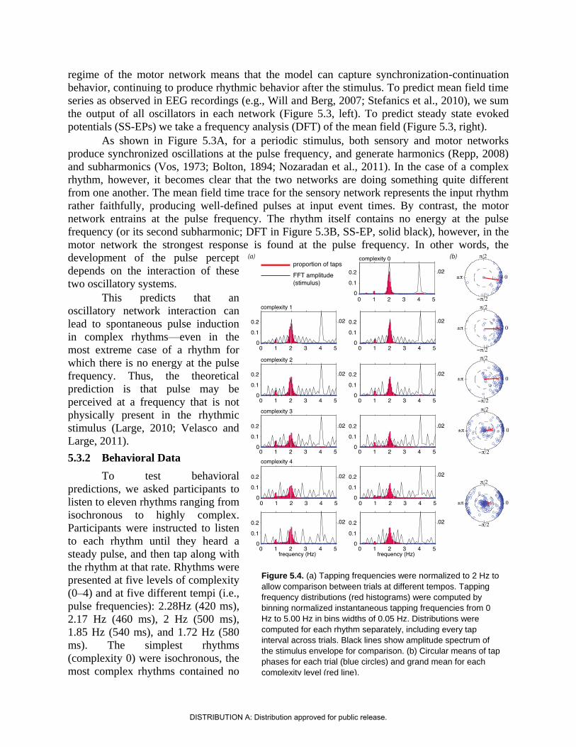
regime of the motor network means that the model can capture synchronization-continuation

behavior, continuing to produce rhythmic behavior after the stimulus. To predict mean field time

series as observed in EEG recordings (e.g., Will and Berg, 2007; Stefanics et al., 2010), we sum

the output of all oscillators in each network (Figure 5.3, left). To predict steady state evoked

potentials (SS-EPs) we take a frequency analysis (DFT) of the mean field (Figure 5.3, right).

As shown in Figure 5.3A, for a periodic stimulus, both sensory and motor networks

produce synchronized oscillations at the pulse frequency, and generate harmonics (Repp, 2008)

and subharmonics (Vos, 1973; Bolton, 1894; Nozaradan et al., 2011). In the case of a complex

rhythm, however, it becomes clear that the two networks are doing something quite different

from one another. The mean field time trace for the sensory network represents the input rhythm

rather faithfully, producing well-defined pulses at input event times. By contrast, the motor

network entrains at the pulse frequency. The rhythm itself contains no energy at the pulse

frequency (or its second subharmonic; DFT in Figure 5.3B, SS-EP, solid black), however, in the

motor network the strongest response is found at the pulse frequency. In other words, the

development of the pulse percept

depends on the interaction of these

two oscillatory systems.

This predicts that an

oscillatory network interaction can

lead to spontaneous pulse induction

in complex rhythms—even in the

most extreme case of a rhythm for

which there is no energy at the pulse

frequency. Thus, the theoretical

prediction is that pulse may be

perceived at a frequency that is not

physically present in the rhythmic

stimulus (Large, 2010; Velasco and

Large, 2011).

5.3.2 Behavioral Data

To test behavioral

predictions, we asked participants to

listen to eleven rhythms ranging from

isochronous to highly complex.

Participants were instructed to listen

to each rhythm until they heard a

steady pulse, and then tap along with

the rhythm at that rate. Rhythms were

presented at five levels of complexity

(0–4) and at five different tempi (i.e.,

pulse frequencies): 2.28Hz (420 ms),

2.17 Hz (460 ms), 2 Hz (500 ms),

1.85 Hz (540 ms), and 1.72 Hz (580

ms). The simplest rhythms

(complexity 0) were isochronous, the

most complex rhythms contained no

Figure 5.4. (a) Tapping frequencies were normalized to 2 Hz to

allow comparison between trials at different tempos. Tapping

frequency distributions (red histograms) were computed by

binning normalized instantaneous tapping frequencies from 0

Hz to 5.00 Hz in bins widths of 0.05 Hz. Distributions were

computed for each rhythm separately, including every tap

interval across trials. Black lines show amplitude spectrum of

the stimulus envelope for comparison. (b) Circular means of tap

phases for each trial (blue circles) and grand mean for each

complexity level (red line).


spectral energy at the pulse frequency (complexity 4). Different combinations of tempo and

rhythm were presented in a pseudorandom order such that consecutive trials always had different

rhythms, and different tempos. Thus, participants were forced to find both the frequency and the

phase of the pulse anew for each rhythm; they could not simply tap at the same tempo

throughout the experiment.

We measured instantaneous tapping frequency distributions to determine whether

subjects induced a pulse at the intended frequency. Instantaneous tapping frequency was

computed as 1/ITI (ITI = inter-tap interval in seconds) and tapping frequencies were normalized

to a frequency of 2 Hz so they could be combined into a single distribution at each level of

complexity. Spectral analysis (DFT) of the stimulus rhythms (Figure 5.4A, black) shows that at

the hypothetical pulse frequency amplitude decreases with increasing complexity. At complexity

level 4, the amplitude is precisely zero at 2 and 1 Hz for each rhythm. Normalized instantaneous

tapping frequency (Figure 5.4A, red histogram) displays a main peak at the normalized pulse

frequency of 2Hz for all rhythms at all levels of complexity, with lesser peaks at 1 and 0.5Hz,

and for some rhythms, a diffuse peak around 4Hz. Thus, the participants most often tapped the

predicted pulse frequency even for the most complex rhythms, which had no spectral amplitude

at that frequency.

Next, we examined synchronization for each trial. The sequence of tap times was

converted into a sequence of phases relative to the predicted pulse frequency, and the circular

mean was computed for each trial (Batschelet, 1981; Figure 5.4B; blue circles). The grand mean

was then computed for each complexity level (Figure 5.4B, red line). As predicted by the model,

participants synchronized—either in-phase or anti-phase—predominantly at the missing pulse

frequency. This behavior is consistent with the prediction that formation of the pulse percept

arises due to entrainment of emergent neuronal oscillations. It also rules out the potential

alternatives that synchronization is merely a consequence of a common rhythmic input, or that

the pulse percept may arise due to linear resonance. Theoretically speaking, it is critical to

distinguish the role of a common stimulus frequency from the intrinsic dynamics of an emergent

oscillation (Whittington et al., 2000), and the missing pulse rhythms used here enabled us to

dissociate the two.

5.3.3 Neural Data

The theoretical model also makes strong

physiological predictions that must also be put to

empirical test. The prediction is that in listening to

these ‘missing pulse’ rhythms, the pulse frequency

will be observed in auditory and motor activity

despite its absence from the stimulus acoustics. Fig

5.5 shows MEG data from n=8 participants,

listening passively to two of the complex ‘missing

pulse’ stimuli (MP1 and MP2) used in the model

simulations (Tal et al, submitted). The spectra of

responses from right and left auditory cortices show

the emergence of peaks at the 2Hz ‘missing pulse’

(and in one case its 1Hz subharmonic; p<0.05 for

all relative to adjacent frequencies; regions of

interest selected based on an independent auditory

1 1.5 2 2.5 3 3.5 4 4.5 5

2

4

6

8

10

12

14

16

18

20MP1

Laud

Raud

1 1.5 2 2.5 3 3.5 4 4.5 5

2

4

6

8

10

12

14

16

18

20

MP2

Norm

aliz

ed a

mp

litu

de

Figure 5.5. (a) Synchronized neural activity was

found in left and right auditory cortices in

response to both complex rhythms. (b) Energy

was found at the missing pulse (here, 2 Hz) and

its second subharmonic (1 Hz) consistent

neither of which were present in the stimuli.


localizer task; Source localization performed using SAM beamforming). Moreover, we found

that the magnitude of the ‘missing pulse’ response is correlated with pulse perception across

individuals, such that participants who perceived the pulse quickly had stronger responses than

participants who took longer to perceive a pulse (MP1: r=-0.81, p<0.005; MP2: r=-0.6, p<0.05;

data not shown). These findings confirm the falsifiable physiological predictions of the model,

they show that neural frequencies correspond to listener’s perceptions, and they conclusively rule

out transient or passive explanations of neural synchrony. Thus, this experiment provided strong

evidence for the viability of the model as a theoretical framework for explaining rhythm

perception.

Summary: We have made significant progress in understanding the role of neural

oscillations and the neural structures that support synchronized responses to musical rhythm. Our

neurodynamic model that shows how self-organization of oscillations in interacting sensory and

motor networks could be responsible for the formation of the pulse percept in complex rhythms.

In a pulse synchronization study, we tested the model’s key prediction that pulse can be

perceived at a frequency for which no spectral energy is present in the amplitude envelope of the

acoustic rhythm. The result shows that participants perceive the pulse at the theoretically

predicted frequency. Synchronized neural activity consistent with model predictions has also

been observed in auditory cortex, providing strong evidence for the viability of this theoretical

framework for explaining rhythm perception. Our model is one of the few consistent with

neurophysiological evidence on the role of neural oscillation, and it explains a phenomenon that

other computational models fail to explain. Because it is based on a canonical model, the

predictions hold for an entire family of dynamical systems, not only a specific one. Thus, this

model provides a theoretical link between oscillatory neurodynamics and the induction of pulse

and meter in musical rhythm.

6. Concluding Remarks

In this project, we developed a theoretical framework for auditory neural processing and

auditory perception. We modeled the auditory system as a dynamical system consisting of

oscillatory networks, and auditory perception as stable dynamic patterns formed in the networks

in response to acoustic signals. We developed GrFNNs, generic models that capture the

neurocomputational properties of a family of neurophysiological models using bifurcation theory.

We made significant progress in understanding the signal processing, pattern formation and

plasticity in GrFNNs. We developed three models that exploit these properties to model

important aspects of auditory neurophysiology and auditory perception. Future modeling efforts

based on canonical dynamical systems could bring us closer to understanding fundamental

mechanisms of hearing, communication, and auditory system development.

In addition to these accomplishments, we produced a computational framework for GrFNNs

in Matlab, sped up our computational simulations using GPU acceleration, and created a C++

version of the GrFNN code to develop end-user applications that run on CPUs, GPU, mobile

platforms and embedded devices. We anticipate that this computational framework will power

the next generation of auditory processing hardware and software. In ongoing work, we are

exploring the abilities of such networks to address the auditory scene analysis problem.


Bibliography

Aronson, D. G., Ermentrout, G. B., & Kopell, N. (1990). Amplitude response of coupled

oscillators. Physica D: Nonlinear Phenomena, 41(3), 403-449.

Bruce, I. C., Sachs, M. B., & Young, E. D. (2003). An auditory-periphery model of the effects of

acoustic trauma on auditory nerve responses. The Journal of the Acoustical Society of

America, 113(1), 369-388.

Brunel, N. (2000). Dynamics of sparsely connected networks of excitatory and inhibitory spiking

neurons. Journal of Computational Neuroscience, 8(3), 183-208.

doi:papers2://publication/uuid/A7D84CF5-49C7-41FF-BCDB-B552A936F0F5

Camalet, S., Duke, T., Julicher, F., & Prost, J. (1999). Auditory sensitivity provided by self tuned

critical oscillations of hair cells. Proceedings of the National Academy of Sciences USA,

97, 3183-3188.

Chen, J. L., Penhune, V. B., & Zatorre, R. J. (2008). Listening to Musical Rhythms Recruits

Motor Regions of the Brain. Cerebral Cortex, 18(12), 2844-2854.

doi:10.1093/cercor/bhn042

Childs, L. M., & Strogatz, S. H. (2008). Stability diagram for the forced Kuramoto model. Chaos,

18(4), 043128. doi:papers2://publication/doi/10.1063/1.3049136

Eguìluz, V. M., Ospeck, M., Choe, Y., Hudspeth, A. J., & Magnasco, M. O. (2000). Essential

nonlinearities in hearing. Physical Review Letters, 84(22), 5232.

Fredrickson-Hemsing, L., Ji, S., Bruinsma, R., & Bozovic, D. (2012). Mode-locking dynamics of

hair cells of the inner ear. Physical Review E, 86(2), 021915.

doi:papers2://publication/doi/10.1103/PhysRevE.86.021915

Fujioka, T., Large, E. W., Trainor, L. J., & Ross, B. (2009). Beta and gamma rhythms in human

auditory cortex during musical beat processing. The Neurosciences and Music III:

Disorders and Plasticity. Annals of the New York Academy of Sciences, 1169, 89-92.

Grahn, J. A., & Rowe, J. B. (2009). Feeling the beat: premotor and striatal interactions in

musicians and non-musicians during beat processing. Journal of Neuroscience.

Holmes, P. J., & Rand, D. A. (1978). Bifurcations of the forced van der Pol oscillator. Quarterly

of Applied Mathematics, 35, 495-509.

Hoppensteadt, F. C., & Izhikevich, E. M. (1996). Synaptic organizations and dynamical

properties of weakly connected neural oscillators II: Learning phase information.

Biological Cybernetics, 75, 126-135.

Hoppensteadt, F. C., & Izhikevich, E. M. (1997). Weakly Connected Neural Networks. New

York: Springer.

Iversen, J. R., Repp, B., & Patel, A. D. (2009). Top-down control of rhythm perception

modulates early auditory responses The Neurosciences and Music III: Disorders and

Plasticity. Annals of the New York Academy of Sciences, 1169, 58-73.

Johnson, D. H. (1980). The relationship between spike rate and synchrony in responses of

auditory-nerve fibers to single tones. The Journal of the Acoustical Society of America,

68(4), 1115-1122. doi:papers2://publication/uuid/CC732D14-61C3-4F7C-91FE-

FDF0B533669C

Joris, P. X., Bergevin, C., Kalluri, R., Mc Laughlin, M., Michelet, P., van der Heijden, M., &

Shera, C. A. (2011). Frequency selectivity in Old-World monkeys corroborates sharp

cochlear tuning in humans. Proceedings of the National Academy of Sciences.


Julicher, F. (2001). Mechanical oscillations at the cellular scale. Comptes Rendus De L Academie

Des Sciences Serie Iv Physique Astrophysique, 2(6), 849-860.

Julicher, F., Andor, D., & Duke, T. (2001). Physical basis of two-tone interference in hearing.

Proceedings of the National Academy of Sciences of the United States of America, 98(16),

9080-9085.

Kern, A., & Stoop, R. (2003). Essential role of couplings between hearing nonlinearities.

Physical Review Letters, 91(12), 128101(128104).

Kim, J. C., & Large, E. W. (2015). Signal Processing in Periodically Forced Gradient Frequency

Neural Networks. Frontiers in Computational Neuroscience, 9, 152.

doi:papers2://publication/doi/10.3389/fncom.2015.00152

Langner, G. (1992). Periodicity coding in the auditory system. Hearing Research, 60, 115-142.

Large, E. W., Almonte, F., & Velasco, M. (2010). A canonical model for gradient frequency

neural networks. Physica D: Nonlinear Phenomena, 239(12), 905-911.

doi:10.1016/j.physd.2009.11.015

Large, E. W., Herrera, J. A., & Velasco, M. J. (2015). Neural Networks for Beat Perception in

Musical Rhythm. Frontiers in Systems Neuroscience, 9(224), 583.

doi:papers2://publication/doi/10.1152/jn.00066.2009

Large, E. W., Kozloski, J., & Crawford, J. D. (1998). A dynamical model of temporal processing

in the fish auditory system. Association for Research in Otolaryngology Abstracts,

21(236), 717.

Laudanski, J., Coombes, S., Palmer, A. R., & Sumner, C. J. (2010). Mode-locked spike trains in

responses of ventral cochlear nucleus chopper and onset neurons to periodic stimuli.

Journal of Neurophysiology, 103(3), 1226-1237. doi:Doi 10.1152/Jn.00070.2009

Lee, K. M., Skoe, E., Kraus, N., & Ashley, R. (2009). Selective subcortical enhancement of

musical intervals in musicians. Journal of Neuroscience, 29(18), 5832-5840.

Lerud, K. D., Almonte, F. V., Kim, J. C., & Large, E. W. (2014). Mode-locking neurodynamics

predict human auditory brainstem responses to musical intervals. Hearing Research.

doi:papers2://publication/doi/10.1016/j.heares.2013.09.010

Lerud, K. D., Kim, J. C., Almonte, F. V., Carney, L. H., & Large, E. W. (under revision). A

canonical nonlinear cochlear model. doi:papers2://publication/uuid/E91A62EA-9977-

4D01-9F5E-2267A8277915

McAuley, J., & Jones, M. R. (2003). Modeling effects of rhythmic context on perceived duration:

a comparison of interval and entrainment approaches to short-interval timing. J Exp

Psychol Hum Percept Perform., 29(6), 1102-1125.

Meddis, R., & O'Mard, L. P. (2006). Virtual pitch in a computational physiological model. The

Journal of the Acoustical Society of America, 120(6), 3861-3869.

doi:papers2://publication/uuid/C44D129E-23E4-40ED-86F1-DC65B9494343

Nozaradan, S. (2012). Selective neuronal synchronization to the beat and meter embedded in a

musical rhythm. doi:papers2://publication/uuid/067E72DD-9FD6-466E-B059-

7060BEFA5402

Nozaradan, S., Peretz, I., Missal, M., & Mouraux, A. (2011). Tagging the neuronal entrainment

to beat and meter. Journal of Neuroscience, 31(28), 10234-10240.

Patterson, R. D., Robinson, K., Holdsworth, J., Mckeown, D., Zhang, C., Allerhand, M., . . .

Langner, G. (1992). Complex Sounds and Auditory Images. Auditory Physiology and

Perception, 83, 429-446.


Snyder, J. S., & Large, E. W. (2005). Gamma-band activity reflects the metric structure of

rhythmic tone sequences. Cognitive Brain Research, 24(1), 117-126.

Stefanescu, R., & Jirsa, V. (2008). A Low Dimensional Description of Globally Coupled

Heterogeneous Neural Networks of Excitatory and Inhibitory Neurons. PLoS

Computational Biology, 4(11), e1000219.

Sussman, E., Steinschneider, M., Gumenyuk, V., Grushko, J., & Lawson, K. (2008). The

maturation of human evoked brain potentials to sounds presented at different stimulus

rates. Hearing Research, 236(1–2), 61-79.

doi:http://dx.doi.org/10.1016/j.heares.2007.12.001

Tremblay, K., Billings, C., & Rohila, N. (2004). Speech evoked cortical potentials: effects of age

and stimulus presentation rate. J Am Acad Audiology, 15(3), 226-237.

Will, U., & Berg, E. (2007). Brain wave synchronization and entrainment to periodic acoustic

stimuli. Neuroscience Letters, 424(1), 55-60.

doi:papers2://publication/doi/10.1016/j.neulet.2007.07.036

Zilany, M. S., & Bruce, I. C. (2006). Modeling auditory-nerve responses for high sound pressure

levels in the normal and impaired auditory periphery. Journal of the Acoustical Society of

America, 120(3), 1446.


http://dx.doi.org/10.1016/j.heares.2007.12.001

AFOSR Deliverables Submission Survey

Response ID:7198 Data

1.

Report Type

Final Report

Primary Contact EmailContact email if there is a problem with the report.

[email protected]

Primary Contact Phone NumberContact phone number if there is a problem with the report

860-282-4215

Organization / Institution name

Circular Logic LLC

Grant/Contract TitleThe full title of the funded effort.

Signal Processing, Pattern Formation and Adaptation in Networks of Neural Oscillators

Grant/Contract NumberAFOSR assigned control number. It must begin with "FA9550" or "F49620" or "FA2386".

FA9550-12-10388

Principal Investigator NameThe full name of the principal investigator on the grant or contract.

Dr. Edward W. Large

Program OfficerThe AFOSR Program Officer currently assigned to the award

Dr. Patrick O. Bradshaw

Reporting Period Start Date

08/01/2012

Reporting Period End Date

07/31/2016

Abstract

In this project, we developed a theoretical framework for auditory neural processing and auditoryperception. We modeled the auditory system as a dynamical system consisting of oscillatory networks, andauditory perception as stable dynamic patterns formed in the networks in response to acoustic signals. Wedeveloped GrFNNs, generic models that capture the neurocomputational properties of a family ofneurophysiological models using bifurcation theory. We conducted theoretical analyses of GrFNNs andmade significant progress in understanding the signal processing, pattern formation and plasticity in them.We developed three models that exploit these properties to model important aspects of auditoryneurophysiology and auditory perception: a model of cochlear dynamics, a model of mode-locked neuraloscillation in the human auditory brainstem, and a model of cortical phase locking to auditory rhythms.Future modeling efforts based on canonical dynamical systems could bring us closer to understandingfundamental mechanisms of hearing, communication, and auditory system development. In addition tothese accomplishments, we produced a computational framework for GrFNNs in Matlab, sped up ourcomputational simulations using GPU acceleration, and created a C++ version of the GrFNN code todevelop end-user applications that run on CPUs, GPU, mobile platforms and embedded devices. We


anticipate that this computational framework will power the next generation of auditory processinghardware and software.

Distribution StatementThis is block 12 on the SF298 form.

Distribution A - Approved for Public Release

Explanation for Distribution StatementIf this is not approved for public release, please provide a short explanation. E.g., contains proprietary information.

SF298 FormPlease attach your SF298 form. A blank SF298 can be found here. Please do not password protect or secure the PDF

The maximum file size for an SF298 is 50MB.

Final+Performance+Report+FA95501210388+SF280+1.pdf

Upload the Report Document. File must be a PDF. Please do not password protect or secure the PDF . Themaximum file size for the Report Document is 50MB.

FinalReportV5.pdf

Upload a Report Document, if any. The maximum file size for the Report Document is 50MB.

Archival Publications (published) during reporting period:

New discoveries, inventions, or patent disclosures:Do you have any discoveries, inventions, or patent disclosures to report for this period?

No

Please describe and include any notable dates

Do you plan to pursue a claim for personal or organizational intellectual property?

Changes in research objectives (if any):

Change in AFOSR Program Officer, if any:

Changed Program Officer from Dr. William Larkin to Dr. Patrick Bradshaw Effective June 6,2014

Extensions granted or milestones slipped, if any:

N/A

AFOSR LRIR Number

LRIR Title

Reporting Period

Laboratory Task Manager

Program Officer

Research Objectives

Technical Summary

Funding Summary by Cost Category (by FY, $K)

Starting FY FY+1 FY+2

Salary

Equipment/Facilities

Supplies

Total

Report Document

Report Document - Text Analysis

Report Document - Text AnalysisDISTRIBUTION A: Distribution approved for public release.

http://www.dtic.mil/whs/directives/forms/eforms/sf0298.pdf

http://www.dtic.mil/whs/directives/forms/eforms/sf0298.pdf

http://surveygizmoresponseuploads.s3.amazonaws.com/fileuploads/11364/363557/165-8f3b3d6c7a80913bce3b18084e15afa0_Final%2BPerformance%2BReport%2BFA95501210388%2BSF280%2B1.pdf

http://surveygizmoresponseuploads.s3.amazonaws.com/fileuploads/11364/363557/60-963c2aba2c30756e73bdc69d4bfaf202_FinalReportV5.pdf

Appendix Documents

2. Thank You

E-mail user

Oct 31, 2016 17:02:45 Success: Email Sent to: [email protected]
