Embed Size (px)
Citation preview

A Sines+Transients+Noise AudioRepresentation for Data Compression and
Time/Pitch Scale Modi�cations
Scott N. Levine�
http://webhost.phc.net/ph/scottl
Julius O. Smith III
http://www-ccrma.stanford.edu/~jos
Center for Computer Research in Music and Acoustics (CCRMA)Department of Music, Stanford University
Stanford, CA 94305-8180, USA
Abstract
The purpose of this paper is to demonstrate a low bitrate audio coding algorithmthat allows modi�cations in the compressed domain. The input audio is segregatedinto three di�erent representations: sinusoids, transients, and noise. Each rep-resentation can be individually quantized, and then easily be time-scaled and/orpitch-shifted.
1 Introduction
The goal of this paper is to present a new representation for audio signals that allows forlow bitrate coding while still allowing for high quality, compressed domain, time-scalingand pitch-shifting modi�cations.
In the current MPEG-4 speci�cations, there are compression algorithms that allow fortime and pitch modi�cations, but only at very low bitrates (2-16 kbps) and relatively lowbandwidth (at 8 kHz sampling rate) using sinusoidal modeling or CELP [1]. In this system,we strive for higher quality with higher bitrates (16-48 kbps), while allowing for highbandwidth (44.1 kHz sampling rate) and high quality time and pitch scale modi�cations.
To achieve the data compression rates and wideband modi�cations, we �rst segmentthe audio (in time and frequency) into three separate signals: a signal which models allsinusoidal content with a sum of time-varying sinusoids [2], a signal which models allattack transients present using transform coding, and a Bark-band noise signal [3] which
�Work supported by Bitbop Laboratories.
1
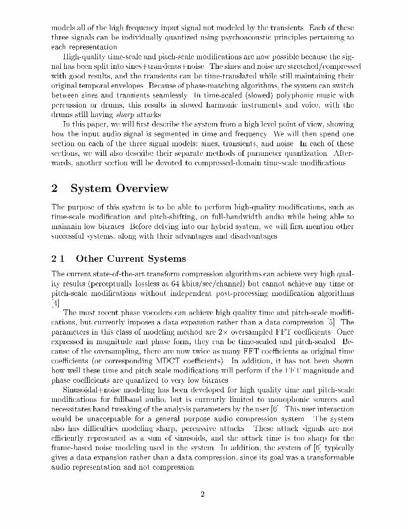
models all of the high frequency input signal not modeled by the transients. Each of thesethree signals can be individually quantized using psychoacoustic principles pertaining toeach representation.
High-quality time-scale and pitch-scale modi�cations are now possible because the sig-nal has been split into sines+transients+noise. The sines and noise are stretched/compressedwith good results, and the transients can be time-translated while still maintaining theiroriginal temporal envelopes. Because of phase-matching algorithms, the system can switchbetween sines and transients seamlessly. In time-scaled (slowed) polyphonic music withpercussion or drums, this results in slowed harmonic instruments and voice, with thedrums still having sharp attacks.
In this paper, we will �rst describe the system from a high level point of view, showinghow the input audio signal is segmented in time and frequency. We will then spend onesection on each of the three signal models: sines, transients, and noise. In each of thesesections, we will also describe their separate methods of parameter quantization. After-wards, another section will be devoted to compressed-domain time-scale modi�cations.
2 System Overview
The purpose of this system is to be able to perform high-quality modi�cations, such astime-scale modi�cation and pitch-shifting, on full-bandwidth audio while being able tomaintain low bitrates. Before delving into our hybrid system, we will �rst mention othersuccessful systems, along with their advantages and disadvantages.
2.1 Other Current Systems
The current state-of-the-art transform compression algorithms can achieve very high qual-ity results (perceptually lossless at 64 kbits/sec/channel) but cannot achieve any time orpitch-scale modi�cations without independent post-processing modi�cation algorithms[4].
The most recent phase vocoders can achieve high quality time and pitch-scale modi�-cations, but currently imposes a data expansion rather than a data compression [5]. Theparameters in this class of modeling method are 2� oversampled FFT coe�cients. Onceexpressed in magnitude and phase form, they can be time-scaled and pitch-scaled. Be-cause of the oversampling, there are now twice as many FFT coe�cients as original timecoe�cients (or corresponding MDCT coe�cients). In addition, it has not been shownhow well these time and pitch-scale modi�cations will perform if the FFT magnitude andphase coe�cients are quantized to very low bitrates.
Sinusoidal+noise modeling has been developed for high quality time and pitch-scalemodi�cations for fullband audio, but is currently limited to monophonic sources andnecessitates hand tweaking of the analysis parameters by the user [6]. This user interactionwould be unacceptable for a general purpose audio compression system. The systemalso has di�culties modeling sharp, percussive attacks. These attack signals are note�ciently represented as a sum of sinusoids, and the attack time is too sharp for theframe-based noise modeling used in the system. In addition, the system of [6] typicallygives a data expansion rather than a data compression, since its goal was a transformableaudio representation and not compression.
2

Sinusoidal modeling has also been used e�ectively for very low bitrate speech [7](2-16kbps/channel) and audio coding [8]. In addition, these systems are able to achieve timeand pitch-scale modi�cations. But these systems were designed for bandlimited (0-4 kHz)monophonic (i.e. single source), signals. If the bandwidth is increased, or a polyphonicinput signal is used, the results are not of su�ciently high quality.
2.2 Time-Frequency Segmentation
It is evident that none of the individual algorithms described in the previous section canhandle both high quality compression and modi�cations. While sinusoidal modeling workswell for steady-state signals, it is not the best representation for attack transients or veryhigh frequencies (above 5 kHz). For this reason, we segment the time-frequency planeinto three general regions: sines, transients, and noise. In each time-frequency region, weuse a di�erent signal representation, and thus di�erent quantization algorithms.
The �rst step in the segmentation is to analyze the signal with a transient detector.The details of the transient detector will be discussed in section 4.1. This step segments,in time, the input signal between attack transients, and non-transient signals. Below 5000Hz, the non-transients are modeled by multiresolution sinusoidal modeling [2], which willbe described in Section 3. Above 5000 Hz, the non-transients are modeled using bark-bandnoise envelopes, similar to those techniques developed in [3], which will be described inSection 5. The transient signals, between 0-16 kHz, are modeled using variants of currenttransform coding techniques [4], which will be described in section 4. This time-frequencysegmentation can be seen in Figure 1. The overlap regions between the sinusoids andthe transients are phase-matched, so no discontinuities can be heard. This will also bediscussed in Section 3. Incremental improvements to the time-frequency segmentationthat allow for lower bitrates and higher �delity synthesis will be described later in thepaper.
2.3 Reasons for the Di�erent Models
Sinusoidal modeling is used only for the non-transient sections of the audio because attacktransients cannot be e�ciently modeled by a set of linearly ramped sinusoids. It is possibleto model transients with a set of sinusoids, but such a system would need hundreds ofsinusoidal parameters, consisting of amplitudes, frequencies, and phases. In this system,we attempt to model only the steady-state signals with sinusoids, thus allowing for ane�cient representation.
Sinusoidal modeling is only used below 5000 Hz because for most music (but not all),there exists very few isolated, tonal sinusoidal elements above 5000 Hz. This is consistentwith results found in the speech world [9]. It is very ine�cient to model high frequencynoise with sinusoids, and it is also very di�cult to track stable, high frequency sinusoidsreliably in loud high-frequency background noise. A residual noise model from 0 to 5kHz is currently being investigated. If one wanted to listen to a pitch pipe or a singleglockenspiel, then there certainly are stable high-frequency sinusoids present. But for mostmusic that people listen to, this is not the case. We could have included an additionaloctave of sinusoids, but this would have added a considerable amount to the total bitrate,and would only bene�t a very small percentage of sound examples.
3
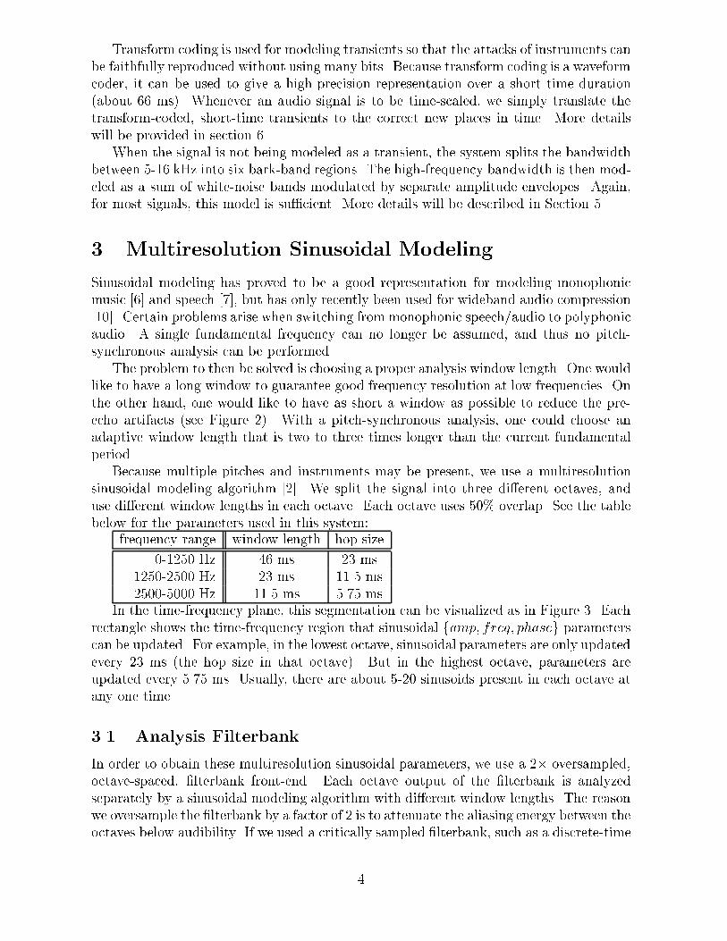
Transform coding is used for modeling transients so that the attacks of instruments canbe faithfully reproduced without using many bits. Because transform coding is a waveformcoder, it can be used to give a high-precision representation over a short time duration(about 66 ms). Whenever an audio signal is to be time-scaled, we simply translate thetransform-coded, short-time transients to the correct new places in time. More detailswill be provided in section 6.
When the signal is not being modeled as a transient, the system splits the bandwidthbetween 5-16 kHz into six bark-band regions. The high-frequency bandwidth is then mod-eled as a sum of white-noise bands modulated by separate amplitude envelopes. Again,for most signals, this model is su�cient. More details will be described in Section 5.
3 Multiresolution Sinusoidal Modeling
Sinusoidal modeling has proved to be a good representation for modeling monophonicmusic [6] and speech [7], but has only recently been used for wideband audio compression[10]. Certain problems arise when switching from monophonic speech/audio to polyphonicaudio. A single fundamental frequency can no longer be assumed, and thus no pitch-synchronous analysis can be performed.
The problem to then be solved is choosing a proper analysis window length. One wouldlike to have a long window to guarantee good frequency resolution at low frequencies. Onthe other hand, one would like to have as short a window as possible to reduce the pre-echo artifacts (see Figure 2). With a pitch-synchronous analysis, one could choose anadaptive window length that is two to three times longer than the current fundamentalperiod.
Because multiple pitches and instruments may be present, we use a multiresolutionsinusoidal modeling algorithm [2]. We split the signal into three di�erent octaves, anduse di�erent window lengths in each octave. Each octave uses 50% overlap. See the tablebelow for the parameters used in this system:
frequency range window length hop size
0-1250 Hz 46 ms 23 ms1250-2500 Hz 23 ms 11.5 ms2500-5000 Hz 11.5 ms 5.75 ms
In the time-frequency plane, this segmentation can be visualized as in Figure 3. Eachrectangle shows the time-frequency region that sinusoidal famp; freq; phaseg parameterscan be updated. For example, in the lowest octave, sinusoidal parameters are only updatedevery 23 ms (the hop size in that octave). But in the highest octave, parameters areupdated every 5.75 ms. Usually, there are about 5-20 sinusoids present in each octave atany one time.
3.1 Analysis Filterbank
In order to obtain these multiresolution sinusoidal parameters, we use a 2� oversampled,octave-spaced, �lterbank front-end. Each octave output of the �lterbank is analyzedseparately by a sinusoidal modeling algorithm with di�erent window lengths. The reasonwe oversample the �lterbank by a factor of 2 is to attenuate the aliasing energy between theoctaves below audibility. If we used a critically sampled �lterbank, such as a discrete-time
4

wavelet transform, each octave output would have aliased energy from the neighboringoctaves. This aliased energy would introduce errors in the sinusoidal modeling. For moredetails on the �lterbank design, see [2][11].
3.2 Sinusoidal Parameters
In each lth frame of analyzed audio, in a given octave, the system produces Rl sets ofplr = fAl
r; !lr; �
lrg (amplitude,frequency,phase) parameters based on maximum likelihood
techniques developed by Thomson [12] and previously used for sinusoidal modeling byHamdy, et al.[10]. For a given frame, indexed by l, the synthesized sound is:
s(m+ lS) =RlX
r=1
Alr cos[m!l
r + �lr] m = 0; : : : ; S � 1
where S is the length of the octave-dependent hop-size, shown in the previous table inSection 3. To be able to synthesize a signal without discontinuities at frame-boundaries,we interpolate the sinusoidal parameters between for each sample m from the observedparameters at m = 0 and m = S. The amplitudes are simply linearly interpolated fromframe to frame. The phase and frequency interpolation will be later be discussed inSection 3.3.
In the next sub-sections, we will show how we �rst track sinusoids from frame to frameand then compute a psychoacoustic masking threshold for each sinusoid. Based on thisinformation, we then decide which sinusoids to eliminate from the system and how toquantize the remaining sinusoids.
3.2.1 Sinusoidal Tracking
Between frame l and (l � 1), the sets of sinusoidal parameters are processed through asimpli�ed peak continuation algorithm. If jAl
i � Al�1j j < Ampthresh and j!l
i � !l�1j j <
Freqthresh then the parameter triads pl�1j and pli are combined into a single sinusoidaltrajectory. If a parameter triad pli cannot be joined with another triad in adjacent frames,fpl�1j ; j = 1; : : : ; Rl�1g and fpl+1k ; k = 1; : : : ; Rl+1g, then this parameter triad becomesa trajectory of length one. With these sets of sinusoidal trajectories, we now begin theprocess of reducing the bits necessary to represent the perceptually relevant information.
3.2.2 Masking
The �rst step in reducing the bitrate for the sinusoids is to estimate how high the sinu-soidal peaks are above the masking threshold of the synthesized signal. In each octaveof sinusoidal modeling, we compute a separate psychoacoustic masking threshold using awindow length equal to the analysis window length for that octave. The model used inthis system was based on the MPEG psychoacoustic model II. For details on computingthe psychoacoustic masking thresholds, see [13].
In each octave, we compute the masking threshold on an approximate third-bark bandscale, or the threshold calculation partition domain in [13]. From 0 to 5 kHz, there areabout 50 non-uniform divisions in frequency that the thresholds are computed within.The ith sinusoidal parameter triad in frame l, pli, then obtains another �eld, the maskingthreshold, ml
i. The masking threshold mli is the di�erence between the energy of the
5

ith sinusoid (correctly scaled to match to domain of the psychoacoustic model) and themasking threshold in its third-bark band [in dB].
Not all of the found sinusoids estimated in the initial analysis [12] are stable sinusoids.We only desire to encode sinusoids that are stable sinusoids, and not model noisy signalswith several closely-spaced sinusoids. We use the psychoacoustic model, which has atonality measure based on prediction of FFT magnitudes and phases, to double-check theresults of the initial sinusoidal estimations.
As can be seen in Figure 4, shorter trajectories have (on average) a lower signal-to-masking threshold. This means that many shorter trajectories will be masked by longer,more stable trajectories. A possible reason for this trend is that the shorter trajectories areattempting to model noise, while the longer trajectories are actually modeling sinusoids.In [13], a stable sinusoid will have a masking threshold at -18 dB in its third-bark band,while a noisy signal will have only a -6 dB masking threshold. Therefore, tonal signals willhave a larger distance to the masking threshold than noisy signals. A simple graphicalexample of the masking thresholds of stable sinusoids can be seen in Figure 5. The signal-to-masking thresholds and trajectory lengths will be important factors in determiningwhich trajectories to eliminate, and how much to quantize the remaining parameters.
3.2.3 Sinusoidal Trajectory Elimination
Not all sinusoidal trajectories found as described Section 3.2.1 will be encoded. A trajec-tory that is masked, meaning its energy was below the masking threshold of its third-barkband, will not be encoded. By eliminating the masked trajectories, the sinusoidal bitrateis decreased approximately 30% in typical audio input signals. In informal listening tests,no audible di�erence was heard after eliminating these trajectories.
3.2.4 Sinusoidal Trajectory Quantization
Once the masked trajectories have been eliminated, the remaining ones are to be quan-tized. In this section, we will concentrate only on amplitude and frequency quantization.We will discuss phase quantization in Section 3.3. Initially, the amplitudes are quantizedwith 5 bits, in increments of 1.5 dB, giving a dynamic range of 96 dB. The frequenciesare quantized to an approximate just noticeable di�erence frequency scale (JNDF) using9 bits.
Because of the slowly varying amplitude and frequency trajectories, we can e�cientlyquantize the temporal �rst-order di�erences across the trajectory. We then Hu�manencode these di�erences. In addition, we can also exploit the inter-trajectory redundancyby Hu�man encoding the di�erence among neighboring trajectories' initial amplitudesand frequencies.
In the previous Section 3.2.3, we eliminated the trajectories that were masked. But,we kept all the other trajectories, even those whose energies were just barely higher thantheir bark-band masking thresholds. In principle, these lower-energy trajectories shouldnot be allocated as many bits as the more perceptually important trajectories; i.e. thosehaving energies much higher than their masking thresholds. A solution that was found tobe bitrate e�cient and which still sounded good was to downsample these lower-energysinusoidal trajectories by a factor of two. That is, update the sinusoidal parameters at halfof the original rate. On the decoder end, the missing parameters are linearly interpolated.
6

This e�ectively reduces the bitrate of these trajectories by 50%, and the total sinusoidalbitrate by an additional 15%.
After testing several kinds of music, we were able to quantize three octaves of multires-olution sinusoids from 0 to 5 kHz at 12-16 kbps. These numbers depend on how much ofthe signal from 0 to 5 kHz is encoded using transient modeling, as discussed in Section 4.More transients per unit time will lower the sinusoidal bitrate, but the transient modelingbitrate will increase.
3.3 Switched Phase Reconstruction
In sinusoidal modeling, transmitting phase information is usually only necessary for oneof two reasons. The �rst reason for keeping phases is to create a residual error signalbetween the original and the synthesized signal. This is needed at the encoder, but notat the decoder. Thus, we need not transmit these phases for this purpose.
The second reason for transmitting phase information is for modeling attack transientswell. During sharp attacks, the phases of sinusoids can be perceptually important. Butin this system, no sharp attacks will be modeled by sinusoids; they will be modeled by atransform coder. Thus, we will not need phase information for this purpose.
A simple example of switching between sines and transients is depicted in Figure 6.At time=40 ms, the sinusoids are cross-faded out and the transients are cross-faded in.Near the end of the transients region at time=90 ms, the sinusoids are cross-faded backin. The trick is to phase-match the sinusoids during the cross-fade in/out times whileonly transmitting the phase information for the frames at the boundaries of the transientregion.
To accomplish this goal, we use cubic polynomial phase interpolation [7] at the bound-aries between the sinusoidal and transient regions. We perform phaseless reconstructionsinusoidal synthesis at all other times. Because we only send phase at transient bound-aries which happen at most several times a second, the contribution of phase informationto the total bitrate is extremely small.
First we will quickly describe the cubic-polynomial phase reconstruction, and thenshow the di�erences between it and phaseless phase reconstruction. Afterwards, we showhow we can switch seamlessly between the two.
3.3.1 Cubic-polynomial Phase Reconstruction
Recall from Section 3.2 that during the lth frame, we estimate the R sets triad of param-eters plr = fAl
r; !lr; �
lrg. These parameters must be interpolated from frame to frame to
eliminate any discontinuities at the frame boundaries. The amplitude is simply linearlyinterpolated from frame to frame.
The phase interpolation is more complicated. We �rst create an instantaneous phaseparameter, �lr, which is a function of surrounding frequencies, f!l
r; !l�1r g and surrounding
phases, f�lr; �
l�1r g. Because the instantaneous phase is derived from four parameters, we
need a cubic polynomial interpolation function. For details of this interpolation function,see [7].
Finally, the reconstruction for frame l becomes
s(m+ lS) =RlX
r=1
Alr(m)cos[�lr(m)] m = 0; : : : ; S � 1 (1)
7

3.3.2 Phaseless Reconstruction
Phaseless reconstruction is called phaseless because it does not need explicit phase in-formation transmitted in order to synthesize the signal. The resulting signal will not bephase aligned with the original signal, but it will not have any discontinuities at frameboundaries.
Instead of deriving the instantaneous phase from surrounding phases and frequen-cies, phaseless reconstruction derives the instantaneous phase as the integral of the in-stantaneous frequency [14]. The instantaneous frequency, !l
r(m), is obtained by linearinterpolation:
!lr(m) = !l�l
r +(!l
r � !l�1r )
Sm m = 0; : : : ; S � 1
Therefore, the instantaneous phase for the rth trajectory in the lth frame is:
�lr(m) = �l�1r + !lr(m) (2)
The term �l�1r refers to the instantaneous phase at the last sample of the previous frame.The signal is then synthesized using Equation (1), but using �lr(m) from Equation (2)instead of the result of a cubic polynomial interpolation function. For the �rst frame ofphaseless reconstruction, the initial instantaneous phase is randomly picked from [��; �).
3.3.3 Phase Switching
In this section, we will show how to switch between phase interpolations algorithmsseamlessly. As a simple example, let the �rst transient begin at frame l. All frames(0; 1; : : : ; l � 2) will be synthesized using the phaseless reconstruction algorithm outlinedin section 3.3.2. During frame l�1, we must seamlessly interpolate between the estimatedparameters f!l�1g and f!l; �lg, using cubic interpolation of Section 3.3.1. Because therewere no estimated phases in frame l � 1, we let �l�1 = �l�1(S), at the last sample of theinstantaneous phase of that frame. In frame l, cubic interpolation is performed betweenf!l; �lg and f!l+1; �l+1g. But, !l = !l+1, and �l+1 can be derived from f!l; �l; Sg, as wasshown in [15]. Therefore, owe need only the phase parameters, �l
r, for r=(1; 2; : : : ; R) foreach transient onset detected.
To graphically describe this scenario, see Figure 7. Each frame is 1024 samples long,and the frames l � 1 and l are shown. That is, the transient begins at t=1024 samples,or the beginning of frame l. A similar algorithm is performed at the end of the transientregion to ensure that the ramped-on sinusoids will be phase matched to the transientbeing ramped-o�.
4 Transform-Coded Transients
Because sinusoidal modeling does not model transients e�ciently, we represent transientswith a short-time transform coder instead. The length of the transform coded sectioncan be varied, but in the current system it is 66 milliseconds. This assumes that mosttransients last less than this amount of time. After the initial attack, most signals be-come somewhat periodic and can be well modeled using sinusoids. First, we will discussour transient detector, which decides when to switch between sinusoidal modeling and
8

transform coding. Then, we describe the basic transform coder used in the system. Inthe following subsection, we then discuss methods to further reduce the number of bitsneeded to encode the transients.
4.1 Transient Detection
The design of the transient detector is very important to the overall performance ofthe system. The transient detector should only ag a transient during attacks that willnot be well modeled using sinusoids. If too many parts of the signal are modeled bytransients, then the bitrate will get too high (transform coding has a higher bitrate thanmultiresolution sinusoidal modeling). In addition, time-scale modi�cation, which will bediscussed in Section 6, will not sound as good. If too few transients are tagged, then someattacks will sound dull and have pre-echo problems due to the limitations of sinusoidalmodeling.
Two methods are combined in the system's transient detection algorithm. The �rstmethod is a conventional frame-based energy measure. It looks for a rising edge in theenergy envelope of the original signal over short frames. The second method involves theresidual signal, which is the di�erence between the original signal and the multiresolutionsinusoidal modeled signal (with cubic polynomial interpolated phase). The second methodmeasures the ratio of short-time energies of the residual and the original signal. If theresidual energy is very small relative to the original energy, then that portion of the signalis most likely tonal and is modeled well by sinusoidal modeling. On the other hand, if theratio is high, it concludes the energy in the original signal was not modeled well by thesinusoids, and an attack transient might be present.
The �nal transient detector uses both methods; i.e., it looks at both rising edges inthe short-time energies of the original signal and also the ratio of residual to originalshort-time energies. The system declares a region to be a transient region when both ofthese methods agree that a transient is occurring.
4.2 A Simpli�ed Transform Coder
The transform coder used in this system is a simpli�ed version of the MPEG-AAC (Ad-vanced Audio Coding) system [4]. It has been simpli�ed to reduce the system's overallcomplexity. The emphasis in this paper is not to improve the current state of the art intransform coding, but rather to use it as a tool to encode transient signals. In the future,we plan to further optimize this simpli�ed coder to reduce the bitrate of the transientsand to introduce a shared bit reservoir pool between the sines, the transients, and thenoise modeling algorithms. In this system, the transient is de�ned as the residual overthe detected transient duration after subtracting out the o�-ramping and on-rampingsinusoids. A graphical example of a transient can be seen in the second plot in Figure 6.
First, the transient is windowed into a series of short (256 point) segments, using araised sine window. At 44.1 kHz, the current system encodes each transient with 24 shortoverlapping 256-point windows, for a total length of 66 ms. There is no window lengthswitching as in AAC since the system has already identi�ed the transient as such. Eachsegment is run through an MDCT [16] to convert from the time domain to a criticallysampled frequency domain. A psychoacoustic model [13] is performed in parallel on the
9

short segments in order to create the masking thresholds necessary for perceptually losslesssubband quantization.
The MDCT coe�cients are then quantized using scale factors and a global gain asin the AAC system. However, there are no iterated rate-distortion loops. We performa single binary search to quantize each scale factor band of MDCT coe�cients to havea mean-squared error just less than the psychoacoustic threshold allows. The resultingquantization noise should now be completely masked. We then use a simpli�ed versionof the AAC noiseless coding to Hu�man encode the MDCT coe�cients, along with thedi�erentially encoded scalefactors.
4.3 Time-Frequency Pruning
In principle, a time duration of a transient is frequency dependent. We do not have arigorous de�nition of transient time duration, other than to generally say it is the timeduring which a signal is not somewhat periodic. At lower frequencies, this time durationis usually longer than it is at higher frequencies.
We mentioned earlier in this section that transients are encoded in this system for 66milliseconds. But because a single transient does not have the same length in time at allfrequencies, we do not need to encode all 66 milliseconds of the transient in every frequencyrange. In particular, we construct a tighter time-frequency range of transform codingaround the attack of the transient. For example, as shown in Figure 8, we transform-encode the signal from 0 to 5 kHz for a total of 66 milliseconds, but we only transformencode the signal from 5-16 kHz for a total of 29 milliseconds. The remaining time-frequency region above 5 kHz not encoded by transform coding is represented by bark-band noise modeling, which will be discussed in the following section.
This pruning of the time-frequency plane greatly reduces the number of bits necessaryto encode transients. As will be shown, bark-band noise modeling is a much lower bitraterepresentation than transform coding. After informal listening tests on many di�erentkinds of music, no di�erences were detected between using transform coding over allfrequency ranges for the full duration of the transient versus just a tighter �t region ofthe time-frequency plane.
As shown in Figure 8, there are only two frequency regions that have di�erent time-widths of transform-encoded transients. This could easily be generalized to more bands,octave-spaced bands, or even a bark-band scale. By using transform coding only aroundthe time-frequency regions that need it, the bitrates can be lowered further. The remainingregions of time-frequency are modeled using multiresolution sinusoidal modeling and bark-band modeling, both of which have lower bitrate requirements.
5 Noise Modeling
In order to reduce the total system bitrate, we stated previously that we will not modelany energy above 5 kHz as tonal (with sinusoids). Above 5 kHz, the signal will either bemodeled as a transform-coded transient or as bark-band �ltered noise, depending on thestate of the transient detector. Bark-band noise modeling bandpass �lters the originalsignal from 5-16 kHz into six bark-spaced bands [17]. This is similar to [3], which modeledthe sinusoidal modeling residual from 0-22 kHz with bark-spaced noise modeling. If a
10

signal is assumed to be noisy, the ear is sensitive only to the total amount of short-timeenergy in a bark band, and not the speci�c distribution of energy within the bark band.Therefore, every 128 samples (3 milliseconds @ 44.1 kHz), an RMS-level energy envelopemeasurement is taken from each of the six bark bandpass �lters. To synthesize the noise,white noise is �ltered through the same bark-spaced �lters and then amplitude modulatedusing the individual energy envelopes.
5.1 Bark-Band Quantization
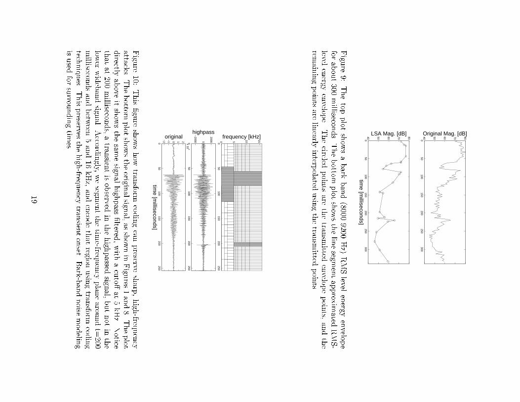
After some informal listening tests, quantizing each bark band energy sample to 1.5 dBseemed the largest possible quantization range possible without hearing artifacts. Anexample of such an envelope can be seen in the top plot of Figure 9. If we Hu�manencode this information, the total data rate would be in the neighborhood of 10 kbps.However, it does not seem perceptually important to sample the energy envelope every128 samples (345 frames/sec). It seems more important perceptually to preserve therising and falling edges of the energy envelopes. Small deviations in the bark-band energyenvelope could be smoothed without audible consequence. The goal is to transmit only asmall subset of the energy envelope points, and linearly interpolate the missing points atthe decoder.
5.2 Line Segment Approximation
We call the samples of the energy envelopes that are transmitted, breakpoints, since theyare points at which the straight lines \break" to change slope. We implemented a greedyalgorithm [18] that iteratively decides where a new breakpoint in the envelope wouldbest minimize the error between the original and approximated envelope. The numberof breakpoints is set to 20% of the length of the envelope itself. Using fewer breakpointswould lower the bitrate, but would introduce audible artifacts in the synthesized noise.An example of an energy envelope reduced by line segment approximation can be seen inthe lower plot of Figure 9.
There are now two sets of data to quantize: the timing and amplitude of the break-points. We Hu�man encode the timing di�erences, along with the amplitude di�erences.In addition, there is another Hu�man table to encode the �rst amplitude of each enve-lope. The initial timing of each envelope can be inferred from timing information of thepreceding transform-coded transient signal. If there is a possibility of losing some data intransmission, the time-di�erential methods will obviously need to be changed. Overall,quantization of the six bands for most signals results in a bitrate of approximately 3 kbps.
5.3 High Frequency Transform Coding
There are certain transients, which we will call microtransients, that are not broadbandor loud enough to be triggered in by the algorithm stated in section 4.1. For example,small drum taps like a closing hi-hat sometimes appears as a microtransients. If thesemicrotransients are modeled by bark-band noise modeling, the result will not sound crisp,but rather distorted and spread. The solution is to use transform coding centered aroundthese attacks, but only from 5 to 16 kHz. Because these high frequency transients are verysudden and short, only three transform coding frames of 128 samples each are necessary.
11

Before and after the sudden transient, bark-band noise modeling is used. See Figure 10for an example and further discussion.
6 Modi�cations
Time-scale and pitch-scale modi�cations are relatively simple to perform on the com-pressed data because the input audio has been segregated into three separate para-metric representations, all of which are well behaved under time/frequency compres-sion/expansion. In this section we will concentrate on time-scale modi�cation. For moredetails on pitch shifting capabilities, see [19]. Because the transients have been separatedfrom the rest of the signal, they can be treated di�erently than the sines or the noise. Inorder to time-scale the audio, the sines and noise components will be stretched in time,while transients will be translated in time. In the next three subsections, we will discussin detail how each of the three models are time-scale modi�ed. See Figures 11 and 12 forgraphical examples and further explanation.
6.1 Sinusoidal Time-Scale Modi�cation
Since the earliest sinusoidal modeling systems for speech and audio, it has been shown howto time-scale the representation. The synthesis equation (1) for the lth frame is slightlyaltered by scaling the hop size S by the time stretch factor �:
s(m + lS�) =RlX
r=1
Alr(m)cos[�lr(m)] m = 0; : : : ; �(S � 1) (3)
When � = 1, no time-stretching is applied. When � > 1, the playback speed is slowed butthe pitch remains the same. Similarly, when � < 1, the playback speed is faster with thesame pitch. The amplitude parameters are still linearly interpolated, but over a di�erentframe length. In addition, the instantaneous phase parameter is now interpolated usingthe phase switching algorithm described in Section 3.3.3 over a di�erent frame length.Even though the cross-fade regions between the sinusoids and the transients now appearat di�erent regions in time, phase-locking is still guaranteed when the sinusoids overlapwith the transient signal.
6.2 Transient Time-scale Modi�cation
To keep the sharp attacks inherent in the transients, the transform-coded transients aretranslated in time rather than stretched in time. Therefore, the MDCT frames are simplymoved to their new place in time and played at the original playback speed. Becausethese signals are so short in time (66 milliseconds), the attack sounds natural and blendswell with the time-stretched sinusoids and noise. Thus, attacks are still sharp, no matterhow much the music has been slowed down.
6.3 Noise Time-scale Modi�cation
Because the noise has been parametrized by envelopes, it is very simple to time-scale thenoise. The breakpoints in the bark band envelopes are stretched according to the time
12

factor, �. Using linear interpolation between the breakpoints, new stretched envelopes areformed. Six channels of bark bandpassed noise are then modulated by these new stretchedenvelopes and summed to form the �nal stretched noise. Similarly, e�cient inverse FFTmethods could be used [3].
7 Acknowledgment
The �rst author would like to thank Tony Verma for his sinusoidal modeling softwarecore, and for many hours of discussions about parametric coders and compression.
8 Conclusions
We described a system that allows both aggressive data compression and high-qualitycompressed-domain modi�cations. By parametrizing sines, transients, and noise sepa-rately, we get the coding gain of perceptually based quantization schemes and the abilityto perform compressed-domain processing. In addition, we can preserve the sharp attacksof transients, even with large time-scale modi�cation factors. To hear demonstrations ofthe data compression and modi�cations described in this paper, see [20].
References
[1] B. Edler, \Current status of the MPEG-4 audio veri�cation model development",Audio Engineering Society Convention, 1996.
[2] S. Levine, T. Verma, and J.O. Smith, \Multiresolution sinusoidal modeling for wide-band audio with modi�cations", Proceedings of the International Conference onAcoustics, Speech, and Signal Processing, Seattle, 1998.
[3] M. Goodwin, \Residual modeling in music analysis-synthesis", Proceedings of theInternational Conference on Acoustics, Speech, and Signal Processing, Atlanta, pp.1005{1008, 1996.
[4] M. Bosi, K. Brandenburg, S. Quackenbush, L.Fielder, K. Akagiri, H.Fuchs, M.Dietz,J.Herre, G.Davidson, and Y.Oikawa, \ISO-IEC MPEG-2 Advanced Audio Coding",Audio Engineering Society Convention, 1996.
[5] J. Laroche and M. Dolson, \Phase-vocoder: About this phasiness business", Pro-ceedings of the IEEE Workshop on Applications of Signal Processing to Audio andAcoustics, New Paltz, NY, 1997.
[6] Xavier Serra and Julius O. Smith III, \Spectral modeling synthesis: A sound analysis/ synthesis system based upon a deterministic plus stochastic decomposition", Comp-uter Music Journal, vol. 14, no. 4, pp. 12{24, winter 1990.
[7] T. Quatieri R. McAulay, \Speech analysis/synthesis based on a sinusoidal represen-tation", IEEE Transactions on Acoustics, Speech, Signal Processing, August 1986.
13

[8] B.Edler, H.Purnhagen, and C. Ferekidis, \ASAC - analysis/synthesis codec for verylow bit rates", Audio Engineering Society Convention, , no. 4179, 1996.
[9] E. Moulines J. Laroche, Y. Styliano, \HNM: A simple, e�cient harmonic + noisemodel for speech", Proceedings of the IEEE Workshop on Applications of SignalProcessing to Audio and Acoustics, New Paltz, NY, 1993.
[10] A. Hamdy, K. Ali and Tew�k H., \Low bit rate high quality audio coding withcombined harmonic and wavelet representations", Proceedings of the InternationalConference on Acoustics, Speech, and Signal Processing, Atlanta, 1996.
[11] U. Zolzer N.J. Fliege, \Multi-complementary �lter bank", Proceedings of the Inter-national Conference on Acoustics, Speech, and Signal Processing, Minneapolis, 1993.
[12] D. J. Thomson, \Spectrum estimation and harmonic analysis", Proceedings of theIEEE, vol. 70, no. 9, pp. 1055{1096, September 1982.
[13] ISE/IEC JTC 1/SC 29/WG 11, \ISO/IEC 11172-3: Information technology - codingof moving pictures and associated audio for digital storage media at up to about 1.5mbit/s - part 3: Audio", 1993.
[14] X. Serra, A System for Sound Analysis/Transformation/Synthsis based on a Deter-mistic plus Stochastic Decomposition, PhD thesis, Stanford University, 1989.
[15] T. Quatieri R. McAulay, \Speech transformations based on a sinusoidal representa-tion", IEEE Transactions on Acoustics, Speech, Signal Processing, vol. 34, December1986.
[16] A. Bradley J. Princen, A. Johnson, \Subband/transform coding using �lter bankdesigns based on time domain aliasing cancellation", pp. 2161{2164, 1987.
[17] E. Zwicker and H. Fastl, Psychoacoustics: Facts and Models, Springer-Verlag, 1990.
[18] J. Beauchamp A. Horner, N. Cheung, \Genetic algorithm optimization of additivesynthsis envelope breakpoints and group synthesis parameters", Proceedings of the1995 International Computer Music Conference, Ban�, pp. 215{222, 1995.
[19] S. Levine, Parametric Audio Representations for Data Compression and Compressed-Domain Processing, PhD thesis, Stanford University, expected December 1998, work-ing title, available online at http://www-ccrma.stanford.edu/~scottl.
[20] S. Levine, \Sound demonstrations for the 1998 San Francisco AES conference",http://webhost.phc.net/ph/scottl/aes98.html.
14

050
100150
200250
−2
−1 0 1 2
x 104
time [m
illiseconds]
amplitude
050
100150
200250
0 2 4 6 8 10 12 14 16
frequency [kHz]
Figu
re1:
Thelow
erplot
show
s250
millisecon
dsof
adrum
attackin
apiece
ofpop
music.
Theupper
plot
show
sthetim
e-frequency
segmentation
ofthissign
al.Durin
gthe
attackportion
ofthesign
al,tran
sformcodingisused
overall
frequencies
andfor
about
66millisecon
ds.Durin
gthenon-tran
sientregion
s,multiresolu
tionsin
usoid
almodelin
gis
used
below
5kHzandbark
-bandnoise
modelin
gisused
from5-16
kHz.
510
1520
2530
35−
1
−0.5 0
0.5 1
synthesized
510
1520
2530
35−
1
−0.5 0
0.5 1
original
510
1520
2530
35−
1
−0.5 0
0.5 1
time [m
illiseconds]
error
Figu
re2:
This�gureshow
sthepre-ech
oerror
resultin
gfrom
sinusoid
almodelin
g.Becau
sethesin
usoid
alam
plitu
deislin
earlyram
ped
fromfram
eto
frame,thesynthesized
onset
timeislim
itedbythelen
gthof
theanaly
siswindow
.
15

0 20 40 60 80 100 1200
0.5
1
1.5
2
2.5
3
3.5
4
4.5
5
freq
uenc
y [k
Hz]
time [milliseconds]
Figure 3: The time-frequency segmentation of multiresolution sinusoidal modeling. Eachrectangle shows the update rate of sinusoidal parameters at di�erent frequencies. In thetop octave, parameters are updated every 5.75 ms, while at the lowest octave the updaterate is only 23 ms. Usually, there are 5-20 sets of sinusoidal parameters present in anyone rectangle.
0 5 10 15
−10
−5
0
5
10
15
trajectory length [in frames]
aver
age
mas
king
thre
shol
d [d
B]
Figure 4: This �gure shows how longer sinusoidal trajectories have a higher average max-imum signal-to-masking threshold than shorter trajectories. Or, the longer a trajectorylasts, the higher its signal-to-masking threshold. This data was derived from the top oc-tave of 8 seconds of pop music, where each frame length is approximately 6 millisecondsin length.
16

5 10 15 20 25 30 35 40 45 50
20
40
60
80
100
120
one−third bark scale
Mag
nitu
de [d
B]
sinusoidal magnitudemasking threshold
Figure 5: The original spectral energy versus the masking threshold of three pure sinusoidsat frequencies 500, 1500, 3200 Hz. Notice that the masking threshold is approximately18 dB below their respective sinusoidal peaks.
0 20 40 60 80 100 120−1
0
1
sine
s
0 20 40 60 80 100 120−1
0
1
tran
sien
ts
0 20 40 60 80 100 120−1
0
1
sine
s+tr
ansi
ents
0 20 40 60 80 100 120−1
0
1
orig
inal
time [milliseconds]
Figure 6: This �gure shows how sines and transients are combined. The top plot shows themultiresolution sinusoidal modeling component of the original signal. The sinusoids arefaded-out during the transient region. The second plot shows a transform-coded transient.The third plot shows the sum of the sines plus the transient. For comparison, the bottomplot is the original signal. The original signal has a sung vowel through the entire section,with a snare drum hit occurring at t=60 ms. Notice that between 0 and 30 ms, thesines are not phase-matched with the original signal, but they do become phase-matchedbetween 30-60 ms, when the transient signal is cross-faded in.
17

200400
600800
10001200
14001600
18002000
−1
−0.5 0
0.5 1fram
e #1 frame #2
cubic phase
200400
600800
10001200
14001600
18002000
−1
−0.5 0
0.5 1
linear phase
200400
600800
10001200
14001600
18002000
−1
−0.5 0
0.5 1
error
time [sam
ples]
Figu
re7:
Thetop
signalshow
sasign
alsynthesized
with
phase
param
eters,andthephase
isinterp
olatedbetw
eenfram
eboundaries
usin
gacubicpoly
nom
ialinterp
olationfunction
[7].Themiddlesign
alissynthesized
usin
gnoexplicit
phase
inform
ationexcep
tat
the
transien
tboundary,
which
isat
time=
1024sam
ples.
Theinitial
phase
isran
dom
,and
isoth
erwise
interp
olatedusin
gtheswitch
edmeth
odof
Section
3.3.Over
theshow
ntim
escale
istwofram
es,each
1024sam
ples
long.
Fram
e#1show
sthemiddlesign
alslow
lybecom
ingphase
locked
tothesign
alabove.
Bythebegin
ningof
frame#2,
thetop
two
signals
arephase
locked
.Thebottom
plot
isthedi�eren
cebetw
eenthetop
twosign
als.
050
100150
200250
−2
−1 0 1 2
x 104
time [m
illiseconds]
amplitude
050
100150
200250
0 2 4 6 8 10 12 14 16
frequency [kHz]
Figu
re8:
This�gure
show
show
toprunethetim
e-frequency
plan
efor
transform
coding
ofatran
sient.
Like
Figu
re1,
thelow
erplot
show
s250
millisecon
dsof
adrum
attackin
apiece
ofpop
music.
Theupper
plot
show
sthetim
e-frequency
segmentation
ofthis
signal.
Durin
gtheattack
portion
ofthesign
al,tran
sformcodingisused
forabout66
millisecon
dsbetw
een0to
5kHz,
butfor
only
29millisecon
dsbetw
een5-16
kHz.
By
reducin
gthetim
e-frequency
regionof
transform
coding,
thebitrate
isred
uced
aswell.
Durin
gthenon-tran
sientregion
s,multiresolu
tionsin
usoid
almodelin
gis
used
below
5kHzandbark
-bandnoise
modelin
gisused
from5-16
kHz.
18
050
100150
200250
30040 50 60 70 80
Original Mag. [dB]
050
100150
200250
30040 50 60 70 80
time [m
illiseconds]
LSA Mag. [dB]
Figu
re9:
Thetop
plot
show
sabark
band(8000-9200
Hz)
RMS-level
energy
envelop
efor
about300
millisecon
ds.Thebottom
plot
show
sthelin
esegm
entapprox
imated
RMS-
levelenergy
envelop
e.Thecircled
poin
tsare
thetran
smitted
envelop
epoin
ts,andthe
remain
ingpoin
tsare
linearly
interp
olatedusin
gthetran
smitted
poin
ts.
050
100150
200250
−2000 0
2000
highpass
050
100150
200250
−2
−1 0 1 2
x 104
time [m
illiseconds]
original
050
100150
200250
0 5 10 15
frequency [kHz]
Figu
re10:
This�gure
show
show
transform
codingcan
preserve
sharp
,high
-frequency
attacks.Thebottom
plot
show
stheorigin
alsign
al,as
show
ninFigu
res1and8.
Theplot
directly
above
itshow
sthesam
esign
alhigh
pass-�
ltered,with
acuto�
at5kHz.
Notice
that
at200
millisecon
ds,atran
sientisobserved
inthehigh
passed
signal,
butnot
inthe
lower
widebandsign
al.Accord
ingly,
wesegm
entthetim
e-frequency
plan
earou
ndt=
200millisecon
dsandbetw
een5and16
kHz,andencodethat
regionusin
gtran
sformcoding
techniques.
Thispreserves
thehigh
-frequency
transien
tonset.
Bark
-bandnoise
modelin
gisused
forsurrou
ndingtim
es.
19

50 100 150 200 250
−2
0
2
x 104 original signal
50 100 150 200 250
−2
0
2
x 104sines + transients + noise, α=1
50 100 150 200 250
−2
0
2
x 104 sines, α=1
50 100 150 200 250
−2
0
2
x 104 transients, α=1
50 100 150 200 250−5000
0
5000noise, α=1
time [milliseconds]
50 100 150 200 250 300 350 400 450
−2
0
2
x 104 sines + transients + noise, α=2
50 100 150 200 250 300 350 400 450
−2
0
2
x 104 sines, α=2
50 100 150 200 250 300 350 400 450
−2
0
2
x 104 transients, α=2
50 100 150 200 250 300 350 400 450−5000
0
5000noise, α=2
time [milliseconds]
Figure 11: This set of plots shows how time-scale modi�cation is performed. The originalsignal, shown at top left, shows two transients: �rst a hi-hat cymbal hit, and then a bassdrum hit. There are also vocals present throughout the sample. The left-side plots showthe full synthesized signal at top, and then the sines, transients, and noise independently.They were all synthesized with no time-scale modi�cation, at �=1. The right-side plotsshow the same synthesized signals, but time-scale modi�ed with �=2, or twice as slowwith the same pitch. Notice how the sines and noise are stretched, but the transients aretranslated. Also, the vertical amplitude scale on the bottom noise plots are ampli�ed 15dB for better viewing.
20

0 50 100 150 200 250
−2
−1
0
1
2
x 104
time [milliseconds]
am
plit
ud
e
0 50 100 150 200 2500
2
4
6
8
10
12
14
16
fre
qu
en
cy [
kH
z]
synthesized at the original speed, α=1
0 50 100 150 200 250 300 350 400
−2
−1
0
1
2
x 104
time [milliseconds]
ampl
itude
0 50 100 150 200 250 300 350 4000
2
4
6
8
10
12
14
16
frequ
ency
[kH
z]
synthesized at 2x slower speed, α=2
Figure 12: These �gures show the time-frequency plane segmentations of Figure 11. The�gure on the left is synthesized with no time-scaling, �=1. The �gure on the right isslowed down by a factor of two, i.e. �=2. Notice how the grid spacing of the transformcoded regions are not stretched, but rather shifted in time. However, the time-frequencyregions of the multiresolution sinusoids and the bark-band noise have been stretched intime in the right plot. Each of the rectangles in those regions are now twice as wide intime. The exception to this rule is the bark-band noise modeled within the time spanof the low-frequency transform-coded samples. These bark-band noise parameters areshifted (not stretched), such that they remain synchronized with the rest of the transient.There are no sinusoids during a transform-coded segment.
21