Embed Size (px)
Citation preview
Aerostructural analysis and design optimization of compositeaircraft
by
Graeme James Kennedy
A thesis submitted in conformity with the requirementsfor the degree of Doctor of Philosophy
Graduate Department of Applied Science and EngineeringUniversity of Toronto
Copyright c© 2012 by Graeme James Kennedy
Abstract
Aerostructural analysis and design optimization of composite aircraft
Graeme James Kennedy
Doctor of Philosophy
Graduate Department of Applied Science and Engineering
University of Toronto
2012
High-performance composite materials exhibit both anisotropic strength and stiffness prop-
erties. These anisotropic properties can be used to produce highly-tailored aircraft struc-
tures that meet stringent performance requirements, but these properties also present unique
challenges for analysis and design. New tools and techniques are developed to address some
of these important challenges. A homogenization-based theory for beams is developed to
accurately predict the through-thickness stress and strain distribution in thick composite
beams. Numerical comparisons demonstrate that the proposed beam theory can be used to
obtain highly accurate results in up to three orders of magnitude less computational time
than three-dimensional calculations. Due to the large finite-element model requirements for
thin composite structures used in aerospace applications, parallel solution methods are ex-
plored. A parallel direct Schur factorization method is developed. The parallel scalability
of the direct Schur approach is demonstrated for a large finite-element problem with over
5 million unknowns. In order to address manufacturing design requirements, a novel lami-
nate parametrization technique is presented that takes into account the discrete nature of
the ply-angle variables, and ply-contiguity constraints. This parametrization technique is
demonstrated on a series of structural optimization problems including compliance mini-
mization of a plate, buckling design of a stiffened panel and layup design of a full aircraft
wing. The design and analysis of composite structures for aircraft is not a stand-alone prob-
lem and cannot be performed without multidisciplinary considerations. A gradient-based
aerostructural design optimization framework is presented that partitions the disciplines
into distinct process groups. An approximate Newton–Krylov method is shown to be an
ii
efficient aerostructural solution algorithm and excellent parallel scalability of the algorithm
is demonstrated. An induced drag optimization study is performed to compare the trade-off
between wing weight and induced drag for wing tip extensions, raked wing tips and winglets.
The results demonstrate that it is possible to achieve a 43% induced drag reduction with no
weight penalty, a 28% induced drag reduction with a 10% wing weight reduction, or a 20%
wing weight reduction with a 5% induced drag penalty from a baseline wing obtained from
a structural mass-minimization problem with fixed aerodynamic loads.
iii

Acknowledgements
Many people have helped me over the course of my research. In particular, I am deeply
grateful for the support and guidance of my supervisor, Professor Joaquim Martins. His
knowledge, enthusiasm and vision for aircraft design and optimization have been an inspi-
ration to me. It has been a pleasure to work with him and I look forward to our future
collaborations.
I would also like to thank the other members of my doctoral committee, Professor Chris
Damaren and Professor David Zingg, for their insights and challenging questions that helped
me to examine different perspectives. Thier questions and comments greatly enhanced the
quality of the thesis.
I am very grateful to many of my colleagues both past and present from UTIAS. In
particular, the members of the MDO lab have provided a unique and enjoyable atmosphere
for research. Specifically, I would like to acknowledge Sandy Mader, for his perspective
and helpful suggestions, Gaetan Kenway for his aircraft design advice, Kai James for his
perspective on all things related to topology optimization, and Jason Hicken for his help
with iterative methods and preconditioners.
I would not have started down the road of graduate studies without my parents, who
encouraged me in all my academic efforts and instilled in me the importance of working on
problems that deeply interest you.
Finally, I would not have been able to complete my studies without the loving support of
my wife Sabrina. Thank you for keeping me grounded, making me smile, and always being
supportive.
Graeme James Kennedy
University of Toronto Institute for Aerospace Studies
September, 2012
Contents
List of Figures v
List of Tables vi
List of Symbols and Abbreviations vii
1 Introduction 1
1.1 Thesis outline and contributions . . . . . . . . . . . . . . . . . . . . . . . . . 4
2 A homogenization-based theory for beams 7
2.1 Review of relevant contributions . . . . . . . . . . . . . . . . . . . . . . . . . 9
2.2 The homogenization-based beam theory . . . . . . . . . . . . . . . . . . . . 13
2.3 A finite-element method for the fundamental states . . . . . . . . . . . . . . 26
2.4 Comparison with three-dimensional results . . . . . . . . . . . . . . . . . . . 32
2.5 Conclusions . . . . . . . . . . . . . . . . . . . . . . . . . . . . . . . . . . . . 41
3 Parallel finite-element analysis of shell structures 43
3.1 Finite-element analysis of shell structures . . . . . . . . . . . . . . . . . . . . 44
3.2 Parallel finite-element analysis . . . . . . . . . . . . . . . . . . . . . . . . . . 54
3.3 Parallel solution methods for sparse linear systems . . . . . . . . . . . . . . . 55
3.4 Structural sensitivity analysis . . . . . . . . . . . . . . . . . . . . . . . . . . 72
3.5 Conclusions . . . . . . . . . . . . . . . . . . . . . . . . . . . . . . . . . . . . 76
4 Laminate parametrization 77
4.1 Literature review . . . . . . . . . . . . . . . . . . . . . . . . . . . . . . . . . 78
4.2 The proposed laminate parametrization . . . . . . . . . . . . . . . . . . . . . 81
4.3 Adjacency constraints . . . . . . . . . . . . . . . . . . . . . . . . . . . . . . 87
4.4 Structural optimization studies . . . . . . . . . . . . . . . . . . . . . . . . . 90
4.5 Wing-box optimization . . . . . . . . . . . . . . . . . . . . . . . . . . . . . . 99
i
4.6 Conclusions . . . . . . . . . . . . . . . . . . . . . . . . . . . . . . . . . . . . 107
5 Aerostructural analysis and design optimization 110
5.1 Review of aerostructural optimization . . . . . . . . . . . . . . . . . . . . . . 111
5.2 Aerostructural analysis components . . . . . . . . . . . . . . . . . . . . . . . 114
5.3 Aerostructural solution methods . . . . . . . . . . . . . . . . . . . . . . . . . 121
5.4 Aerostructural gradient evaluation . . . . . . . . . . . . . . . . . . . . . . . . 126
5.5 Aerostructural optimization studies . . . . . . . . . . . . . . . . . . . . . . . 129
5.6 Conclusions . . . . . . . . . . . . . . . . . . . . . . . . . . . . . . . . . . . . 140
6 Contributions, conclusions and future work 144
6.1 Contributions and conclusions . . . . . . . . . . . . . . . . . . . . . . . . . . 144
6.2 Future work . . . . . . . . . . . . . . . . . . . . . . . . . . . . . . . . . . . . 146
6.3 Epilogue . . . . . . . . . . . . . . . . . . . . . . . . . . . . . . . . . . . . . . 148
References 149
A Shell element tests 162
ii
List of Figures
1.1 Approximate composite mass percentage by year of entry into service . . . . 2
1.2 Degrees of freedom required for the structural analysis of a wing . . . . . . . 3
1.3 Connections between the major thesis topics . . . . . . . . . . . . . . . . . . 5
2.1 A comparison between through-thickness shear stress and strain distributions 8
2.2 Geometry of the reference beam . . . . . . . . . . . . . . . . . . . . . . . . . 13
2.3 The fundamental states . . . . . . . . . . . . . . . . . . . . . . . . . . . . . . 19
2.4 The angle section geometry . . . . . . . . . . . . . . . . . . . . . . . . . . . 33
2.5 Sectional strain energy of the difference between theory and finite-element
results . . . . . . . . . . . . . . . . . . . . . . . . . . . . . . . . . . . . . . . 34
2.6 Comparison of the through-thickness volumetric strain at the cross-section
x = L/2 for the statically indeterminate beam . . . . . . . . . . . . . . . . . 35
2.7 Relative errors of the strain moments for the statically determinate beam . . 36
2.8 Relative errors of the strain moments for the statically indeterminate beam . 37
2.9 Relative errors of the stress moments for the statically indeterminate beam . 38
2.10 The moments of the strain residual for the statically determinate beam . . . 39
2.11 Components of the relative strain correction error for the statically determi-
nate beam . . . . . . . . . . . . . . . . . . . . . . . . . . . . . . . . . . . . . 41
3.1 The initial and deformed geometry of a shell segment . . . . . . . . . . . . . 47
3.2 The interpolation scheme for the MITC shell elements . . . . . . . . . . . . . 52
3.3 Condition number of a plate problem for various slenderness ratios . . . . . . 54
3.4 Domain decomposition and matrix for the approximate Schur preconditioner 58
3.5 Domain decomposition and matrix for the direct Schur method . . . . . . . . 61
3.6 The block cyclic matrix data format . . . . . . . . . . . . . . . . . . . . . . . 64
3.7 The annular disk and transonic transport wing finite-element problems . . . 66
3.8 Level of fill and parallel scaling studies for a plane stress problem . . . . . . 67
3.9 Factorization times for the direct Schur approach using various orderings . . 69
iii
3.10 Factor time as a function of the ideal factor time . . . . . . . . . . . . . . . 70
3.11 Solution and assembly times for the direct Schur approach . . . . . . . . . . 72
3.12 Adjoint computational cost assessment . . . . . . . . . . . . . . . . . . . . . 74
4.1 Illustration of the spherical constraint . . . . . . . . . . . . . . . . . . . . . . 84
4.2 Convergence history for the plate compliance problem . . . . . . . . . . . . . 92
4.3 Convergence history for the plate compliance problem with adjacency constraints 92
4.4 The lamination sequences for the compliance minimization problem . . . . . 93
4.5 The lamination sequences for the compliance minimization problem with ad-
jacency constraints . . . . . . . . . . . . . . . . . . . . . . . . . . . . . . . . 94
4.6 The geometry of the buckling optimization problem formulation. . . . . . . . 94
4.7 Optimal lamination sequences for the stiffened panel optimizations . . . . . . 97
4.8 Convergence history of the stiffened panel optimizations . . . . . . . . . . . . 98
4.9 Function evaluations required for the stiffened panel optimizations . . . . . . 98
4.10 The number of plies for the top and bottom skin and stiffener, and the top
and bottom the stiffener heights and stiffener base-widths. . . . . . . . . . . 103
4.11 An illustration of the global-local wing-box analysis . . . . . . . . . . . . . . 104
4.12 The continuation history of the load factor, λ, and the infeasibility ||cs(x∗n)−e||1 for the wing-box optimization. . . . . . . . . . . . . . . . . . . . . . . . 106
4.13 The number of function evaluations and gradient evaluations required for the
wing-box optimization. . . . . . . . . . . . . . . . . . . . . . . . . . . . . . . 106
4.14 Ply angle sequences for the wing-box optimization problem. Only the top half
of the symmetric laminate is shown. . . . . . . . . . . . . . . . . . . . . . . . 109
5.1 Timing results for analysis and sensitivity evaluation using TriPan with a
14 400 surface panel mesh . . . . . . . . . . . . . . . . . . . . . . . . . . . . 116
5.2 Verification of TriPan against SUmb for the ONERA M6 at M = 0.5 and
α = 3.06. . . . . . . . . . . . . . . . . . . . . . . . . . . . . . . . . . . . . . . 117
5.3 The initial and final geometry obtained using FFD approach . . . . . . . . . 122
5.4 Comparison of solution times for the ANK 1 and ANK 2 aerostructural solu-
tion methods . . . . . . . . . . . . . . . . . . . . . . . . . . . . . . . . . . . 126
5.5 Comparison of computational times for different parts of the aerostructural
sensitivity analysis . . . . . . . . . . . . . . . . . . . . . . . . . . . . . . . . 128
5.6 Aerostructural sensitivity verification . . . . . . . . . . . . . . . . . . . . . . 129
5.7 Summary of the results from all the induced drag minimization studies . . . 137
5.8 A comparison of the optimal planforms . . . . . . . . . . . . . . . . . . . . . 138
iv
5.9 The t/c distribution for the span extension results . . . . . . . . . . . . . . . 139
5.10 Thickness and stiffener height distributions for the span extension cases . . . 142
5.11 Twist and clc distributions for the span extension cases . . . . . . . . . . . . 143
A.1 Displacement and MITC-based shell element accuracy study for a plate . . . 163
A.2 Displacement and MITC-based shell element accuracy study for a cylinder . 163
A.3 A test of the MITC shell elements for the snap-through of a partial cylinder
and the pressure-buckling of a full cylinder . . . . . . . . . . . . . . . . . . . 164
v
List of Tables
2.1 Representative orthotropic stiffness properties . . . . . . . . . . . . . . . . . 32
4.1 Representative IM7/3501-6 stiffness and strength properties. . . . . . . . . . 90
4.2 Design problem summary for the buckling optimization studies . . . . . . . . 96
4.3 Wing-box mass breakdown . . . . . . . . . . . . . . . . . . . . . . . . . . . . 103
5.1 Levels of parallelism and process groups within the aerostructural optimiza-
tion framework. . . . . . . . . . . . . . . . . . . . . . . . . . . . . . . . . . . 114
5.2 Summary of the design variables in the aerostrucutral induced drag study . . 132
5.3 Summary of the constraints in the aerostrucutral induced drag study . . . . 133
vi

List of Symbols and Abbreviations
Abbreviations
AMD Approximate Minimum Degree
BILU Block-Incomplete LU-factorization
BWB Blended Wing Body
CAD Computer Aided Design
CLT Classical Lamination Theory
DMO Discrete Material Optimization
FFD Free Form Deformation
F-GCROT Flexible-GCROT
F-GMRES Flexible-GMRES
FSDT First-order Shear Deformation Theory
GA Genetic Algorithm
GCROT Generalized Conjugate Residual with inner-Orthogonalization
and outer Truncation
GMRES Generalized Minimum RESidual
ILU Incomplete LU-factorization
KS Kreisselmeier–Steinhauser (constraint aggregation technique)
LICQ Linear-Independence Constraint Qualification
MDO Multidisciplinary Design Optimization
MFCQ Mangasarian–Fromovitz Constraint Qualification
MITC Mixed Interpolation of Tensorial Components
MTOW Maximum TakeOff Weight
ND Nested Disection
OML Outer Mould Line
RCM Reverse Cuthill–McKee
SIMP Solid Isotropic Microstructure with Penalization
vii
SNOPT Sparse Nonlinear OPTimizer (software)
SUmb Stanford University multi-block solver
TACS Toolkit for the Analysis of Composite Structures
Chapter 2
A The cross-sectional area
C The constitutive matrix
Cs The strain moment correction matrix
D The homogenized stiffness matrix
E The homogenized flexibility matrix
ε The strain
ε The strain residuals
ε(k)F The primary fundamental states
ε(k)LF The load-dependent fundamental states
e The strain moments
e The moments of the strain produced by the displacement residuals
e(k)FL The load-dependent strain moment correction
Iz, Iy The second moments of area
Ks The stress moment correction matrix
L0 The normalized displacement operator
Ls The stress and strain moment operator
Lε The average strain operator
σ The stress
σ The stress residuals
σ(k)F The primary fundamental states
σ(k)LF The load-dependent fundamental states
s The stress moments
s(k)FL The load-dependent stress moment correction
u The displacements
u The residual displacements
u0 The normalized displacement moments
viii
Chapter 3
A A sparse matrix
b, x The right-hand-side and solution vector
C The constitutive tensor
ε The Green strain
η The shell volume parameters
f(u,x) A vector of functions of interest
φ Small rotations in the global Cartesian frame
ψ The adjoint vector
∇xf The total derivative of a vector of functions of interest
Q The shell-normal rotation matrix
r The mid-surface of the shell
R The shell volume position vector
S The second Piola–Kirchhoff stress tensor
u The displacement of the mid-surface
U The through-thickness displacement
ω The rate of change of the displacements through the thickness
ξ1, ξ2 The shell surface parameters
ζ The through-thickness parameter
Chapter 4
A(i), B(i), D(i), A(i)s The constitutive matrices
Aw The ply-angle selection variable weighting matrix
cs(x) The spherical constraints
d(x) The grouped adjacency constraints
∆cr The critical end shortening
f(x) The design objective
F(i)KS The aggregated failure envelope
γ The penalization parameter
Ik The set of excluded design variable selections
τ The regularization parameter
xijk The ply-angle selection variables
ix

x The full set of ply-angle selection variables
Chapter 5
b The wing span
C(a, ϕ) A rotation matrix
Di Induced drag
e The span efficiency factor
F Consistent structural force vector due to aerodynamic loads
L Aerodynamic lift
ψ The aerostructural adjoint vector
q The aerostructural state variables
R The aerostructural residuals
RS The structural residuals
RA The aerodynamic residuals
u The structural state variables
w The aerodynamic state variables
x The aerostructural design variables
Xs The aerodynamic surface nodes
x
Chapter 1
Introduction
Composite materials are fabricated using a macroscopic combination of two or more con-
stituent materials such that the overall structural properties of the composite are superior
to the properties of the individual component materials. In aerospace applications, high-
performance composites are often made from carbon fibers set in an epoxy matrix. These
high-performance composite materials exhibit both highly anisotropic strength and stiff-
ness properties, making the analysis and design of composite structures more challenging.
However, the anisotropic properties of composite materials can also be exploited to obtain
tailored structures that meet stringent design requirements, yet are lighter than equivalent
metallic structures. Fully exploiting the anisotropic nature of composites often requires new
analysis methods and new design methodologies.
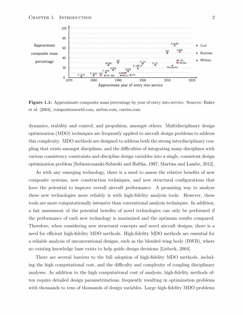
Over the years, new aircraft designs have employed increasing amounts of composite
materials. Figure 1.1 shows the usage of composite materials in both civil and military
aircraft over several decades. This trend is due in part to the higher stiffness-to-weight
and strength-to-weight ratios exhibited by composite materials when compared to metallic
structures. Additionally, composites may have manufacturing benefits. For example, using
composite manufacturing techniques, a large complex structural component can be manu-
factured in a single piece. This part-count reduction can save both weight and maintenance
costs [Baker et al., 2004]. Currently, composite materials are being used for highly-loaded,
primary structures in civil aircraft, including the Bombardier CSeries wing, the Boeing 787
wing and fuselage, and the Airbus A350 wing and fuselage. Yet these applications have not
come without considerable investment in research and development over the past 50 years.
The design and analysis of composite structures for aircraft, however, is not a stand-alone
problem and thus cannot be performed in isolation. Aircraft are complex, coupled systems
that require the simultaneous consideration of multiple disciplines, such as structures, aero-
1
Chapter 1. Introduction 2
0
20
40
60
80
100
1970 1980 1990 2000 2010 2020
Approximate year of entry into service
Approximate
composite mass
percentage
Civil
Business
Military
F-15A F-16AF-18A
AV8BB2
F-18E/F
V-22F-22
F-35
767737-300
A320
MD11A340
A330
777
787 A350
CSeries
HondaJet
Lear85
Figure 1.1: Approximate composite mass percentage by year of entry into service. Sources: Baker
et al. [2004], compositesworld.com, airbus.com, cseries.com
dynamics, stability and control, and propulsion, amongst others. Multidisciplinary design
optimization (MDO) techniques are frequently applied to aircraft design problems to address
this complexity. MDO methods are designed to address both the strong interdisciplinary cou-
pling that exists amongst disciplines, and the difficulties of integrating many disciplines with
various consistency constraints and discipline design variables into a single, consistent design
optimization problem [Sobieszczanski-Sobieski and Haftka, 1997, Martins and Lambe, 2012].
As with any emerging technology, there is a need to assess the relative benefits of new
composite systems, new construction techniques, and new structural configurations that
have the potential to improve overall aircraft performance. A promising way to analyze
these new technologies more reliably is with high-fidelity analysis tools. However, these
tools are more computationally intensive than conventional analysis techniques. In addition,
a fair assessment of the potential benefits of novel technologies can only be performed if
the performance of each new technology is maximized and the optimum results compared.
Therefore, when considering new structural concepts and novel aircraft designs, there is a
need for efficient high-fidelity MDO methods. High-fidelity MDO methods are essential for
a reliable analysis of unconventional designs, such as the blended wing body (BWB), where
no existing knowledge base exists to help guide design decisions [Liebeck, 2004].
There are several barriers to the full adoption of high-fidelity MDO methods, includ-
ing the high computational cost, and the difficulty and complexity of coupling disciplinary
analyses. In addition to the high computational cost of analysis, high-fidelity methods of-
ten require detailed design parametrizations, frequently resulting in optimization problems
with thousands to tens of thousands of design variables. Large high-fidelity MDO problems
Chapter 1. Introduction 3
Model complexity
Degreesoffreedom
102
104
106
108
1010
1012
Beam model
Shell model
Full 3D model
Metallic wing
Composite wing
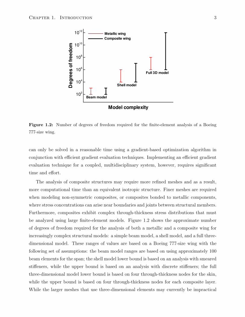
Figure 1.2: Number of degrees of freedom required for the finite-element analysis of a Boeing
777-size wing.
can only be solved in a reasonable time using a gradient-based optimization algorithm in
conjunction with efficient gradient evaluation techniques. Implementing an efficient gradient
evaluation technique for a coupled, multidisciplinary system, however, requires significant
time and effort.
The analysis of composite structures may require more refined meshes and as a result,
more computational time than an equivalent isotropic structure. Finer meshes are required
when modeling non-symmetric composites, or composites bonded to metallic components,
where stress concentrations can arise near boundaries and joints between structural members.
Furthermore, composites exhibit complex through-thickness stress distributions that must
be analyzed using large finite-element models. Figure 1.2 shows the approximate number
of degrees of freedom required for the analysis of both a metallic and a composite wing for
increasingly complex structural models: a simple beam model, a shell model, and a full three-
dimensional model. These ranges of values are based on a Boeing 777-size wing with the
following set of assumptions: the beam model ranges are based on using approximately 100
beam elements for the span; the shell model lower bound is based on an analysis with smeared
stiffeners, while the upper bound is based on an analysis with discrete stiffeners; the full
three-dimensional model lower bound is based on four through-thickness nodes for the skin,
while the upper bound is based on four through-thickness nodes for each composite layer.
While the larger meshes that use three-dimensional elements may currently be impractical
Chapter 1. Introduction 4
for design, they illustrate an upper bound on the size of the structural model.
As Figure 1.2 illustrates, using high-fidelity models for analysis and design optimiza-
tion involves solving large finite-element problems that require significant computational
resources. These large problems can only be solved in a practical time frame if efficient
parallel methods can be employed. Furthermore, gradient-based optimization methods for
structural design optimization with parametrizations that require thousands to tens of thou-
sands of design variables are only practical if accurate and efficient derivative evaluation
methods, such as the adjoint method, are employed. In order to address these requirements
I have developed a parallel finite-element code specifically designed for multidisciplinary de-
sign optimization of composite structures. This finite-element code, called the Toolkit for
the Analysis of Composite Structures (TACS), includes routines that enable accurate and
efficient analytic derivative computation, an essential tool for gradient-based design opti-
mization. In addition, TACS is designed to efficiently couple with other disciplines for both
analysis and multidisciplinary derivative computations.
The goal of this thesis is to address challenging problems in the areas of composite struc-
tural analysis and design, and in the area of aerostructural design optimization of composite
aircraft structures. In order to make progress towards this goal, I have developed new
analysis methods for composites, I have refined numerical algorithms for solving large finite-
element problems, and I have applied multidisciplinary design analysis and optimization
methods to the design of composite aircraft structures. In this thesis, I have focused on the
analysis and design of composite wing box structures for large transport aircraft. However,
the techniques presented within this thesis are more broadly applicable to other composite
design problems. Furthermore, I have also focused on applications that use high-strength
carbon epoxy composite systems, which are commonly used in transport aircraft structures.
However, many of the results could also be applied to other laminated composite systems
with different material properties.
1.1 Thesis outline and contributions
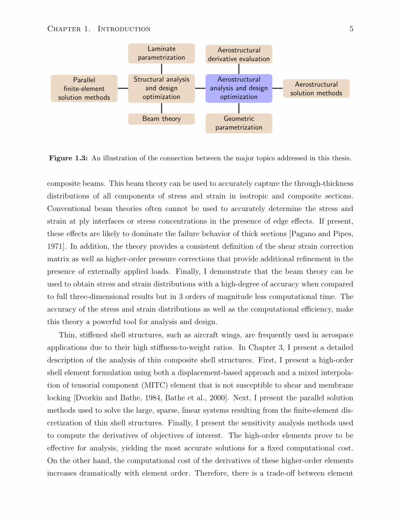
The connections between the major topics addressed in this thesis are illustrated in Fig-
ure 1.3. The central goal is to enhance aerostructural analysis and design optimization
methods for composite aircraft. This topic, however, cannot be approached without also
addressing other topics that are closely related.
Accurate stress and strain distributions are required to predict the failure properties
of composite structures. In Chapter 2, I present a novel beam theory for isotropic and
Chapter 1. Introduction 5
Aerostructuralanalysis and design
optimization
Structural analysisand design
optimization
Laminateparametrization
Parallelfinite-element
solution methods
Beam theory Geometricparametrization
Aerostructuralsolution methods
Aerostructuralderivative evaluation
Figure 1.3: An illustration of the connection between the major topics addressed in this thesis.
composite beams. This beam theory can be used to accurately capture the through-thickness
distributions of all components of stress and strain in isotropic and composite sections.
Conventional beam theories often cannot be used to accurately determine the stress and
strain at ply interfaces or stress concentrations in the presence of edge effects. If present,
these effects are likely to dominate the failure behavior of thick sections [Pagano and Pipes,
1971]. In addition, the theory provides a consistent definition of the shear strain correction
matrix as well as higher-order pressure corrections that provide additional refinement in the
presence of externally applied loads. Finally, I demonstrate that the beam theory can be
used to obtain stress and strain distributions with a high-degree of accuracy when compared
to full three-dimensional results but in 3 orders of magnitude less computational time. The
accuracy of the stress and strain distributions as well as the computational efficiency, make
this theory a powerful tool for analysis and design.
Thin, stiffened shell structures, such as aircraft wings, are frequently used in aerospace
applications due to their high stiffness-to-weight ratios. In Chapter 3, I present a detailed
description of the analysis of thin composite shell structures. First, I present a high-order
shell element formulation using both a displacement-based approach and a mixed interpola-
tion of tensorial component (MITC) element that is not susceptible to shear and membrane
locking [Dvorkin and Bathe, 1984, Bathe et al., 2000]. Next, I present the parallel solution
methods used to solve the large, sparse, linear systems resulting from the finite-element dis-
cretization of thin shell structures. Finally, I present the sensitivity analysis methods used
to compute the derivatives of objectives of interest. The high-order elements prove to be
effective for analysis, yielding the most accurate solutions for a fixed computational cost.
On the other hand, the computational cost of the derivatives of these higher-order elements
increases dramatically with element order. Therefore, there is a trade-off between element
Chapter 1. Introduction 6
order and accuracy of the solution and the computational cost of the gradients for design
optimization.
Design optimization of composite structures cannot be performed without a flexible de-
sign parametrization that can take into account important manufacturing requirements.
In Chapter 4, I present a parametrization technique for laminated composite structures.
This parametrization takes into account the discrete nature of the ply-angle variables that
may arise due to manufacturing constraints. Often these ply parametrization problems are
solved with gradient-free approaches [Haftka and Walsh, 1992, Le Riche and Haftka, 1993,
Adams et al., 2004], however, this parametrization results in a continuous formulation that
is amenable to gradient-based design optimization. The proposed parametrization uses an
exact penalty function to ensure that there are no intermediate plies in the final design. I also
present additional constraints that can be used to enforce other manufacturing requirements
such as a restriction on the number of contiguous plies at the same angle, or that adjacent
ply angles be restricted to a reduced set of values.
In Chapter 5, I present an aerostructural optimization framework, focusing in partic-
ular on the parallel computational aspects of the approach. Previous authors have used
high-fidelity aerodynamic models coupled to low or medium fidelity structural finite-element
models [Martins et al., 2004, Maute et al., 2001]. This imbalance may be acceptable if the pri-
mary interest is the aerodynamic performance of the flying, displaced shape of a conventional
wing. However, more detailed effects, such as the skin-bulge due to the internal pressure for
a BWB [Liebeck, 2004, Hansen et al., 2008], can only be assessed using high-fidelity models.
In addition, low-fidelity models such as a simple beam model, cannot always be relied on to
provide detailed stress distributions or accurate weight estimates for novel configurations or
even novel structural composite technologies. For instance, it would be difficult to assess the
benefits of a composite system such as the new structural concept PRSEUS [Jegley et al.,
2002, Velicki and Thrash, 2008, Li and Velicki, 2008], for a BWB configuration using only
a beam model, or even a coarse shell model. As a first step towards this goal, I examine
methods in which high-fidelity, finite-element structural analysis is coupled to a medium-
fidelity aerodynamic tool. In particular, I examine solution methods for problems in which
both the aerodynamic and structural analyses are performed in parallel and where both re-
quire significant computational time. Finally, using the proposed aerostructural framework,
I present results for a series of non-planar configurations and draw conclusions about their
relative benefits.
Chapter 2
A homogenization-based theory for
beams
Beam theories are developed based on a set of assumptions that are used to reduce the
complex behavior of a slender, three-dimensional body to an equivalent one-dimensional
problem. The usefulness of a beam theory should be assessed based on its range of appli-
cability, the accuracy of its results, and the complexity of the analysis required to obtain
results. In this chapter, I present a homogenization based theory for anisotropic beams. This
homogenization-based theory is based on a series of novel contributions to beam theory orig-
inally conceived by Hansen and Almeida [2001] and Hansen et al. [2005] and applied to the
analysis of layered beams under conditions of plane stress. While the assumptions used to
derive this homogenization-based theory differ significantly from classical assumptions, the
proposed beam theory takes a form similar in many respects to classical Timoshenko beam
theory [Timoshenko, 1921, 1922]. This homogenization-based theory, however, is specifically
designed for composite beams. In the homogenization-based approach, the stiffness prop-
erties, shear strain correction matrix, and load-dependent corrections within the theory are
calibrated based on a hierarchy of solutions called the fundamental states. The fundamen-
tal states are accurate sectional stress and strain solutions to a series of carefully-chosen,
statically determinate beam problems. Since it is difficult to obtain exact solutions for the
fundamental states for an arbitrary section, I formulate a finite-element solution technique
to obtain approximate solutions.
There are several difficulties that arise when developing a beam theory for the analysis of
composite beams. To illustrate the most significant challenges, consider the four layer beam
illustrated in Figure 2.1. This two-dimensional beam is composed of alternating layers of two
materials, where one material has a shear modulus that is 10 times higher than the other.
7
Chapter 2. A homogenization-based theory for beams 8
Actual
strain stress
Timoshenko
strain stress
Higher-order
strain stressz
0.1 G
G
0.1G
G
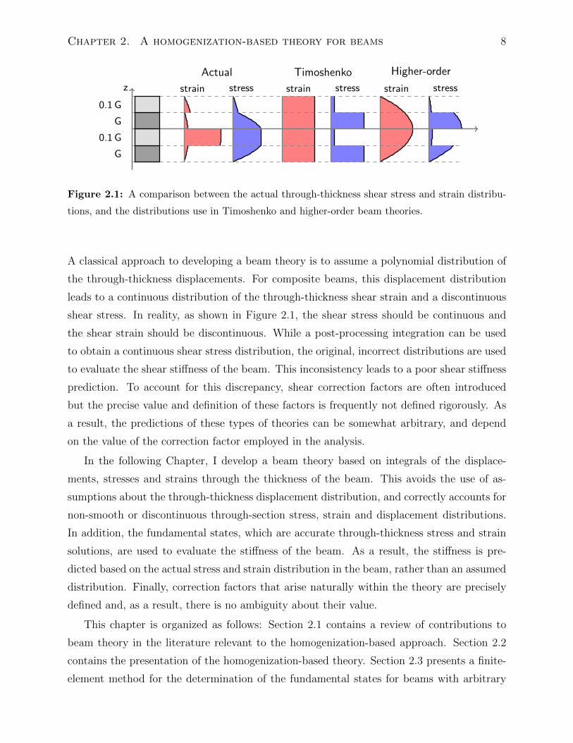
Figure 2.1: A comparison between the actual through-thickness shear stress and strain distribu-
tions, and the distributions use in Timoshenko and higher-order beam theories.
A classical approach to developing a beam theory is to assume a polynomial distribution of
the through-thickness displacements. For composite beams, this displacement distribution
leads to a continuous distribution of the through-thickness shear strain and a discontinuous
shear stress. In reality, as shown in Figure 2.1, the shear stress should be continuous and
the shear strain should be discontinuous. While a post-processing integration can be used
to obtain a continuous shear stress distribution, the original, incorrect distributions are used
to evaluate the shear stiffness of the beam. This inconsistency leads to a poor shear stiffness
prediction. To account for this discrepancy, shear correction factors are often introduced
but the precise value and definition of these factors is frequently not defined rigorously. As
a result, the predictions of these types of theories can be somewhat arbitrary, and depend
on the value of the correction factor employed in the analysis.
In the following Chapter, I develop a beam theory based on integrals of the displace-
ments, stresses and strains through the thickness of the beam. This avoids the use of as-
sumptions about the through-thickness displacement distribution, and correctly accounts for
non-smooth or discontinuous through-section stress, strain and displacement distributions.
In addition, the fundamental states, which are accurate through-thickness stress and strain
solutions, are used to evaluate the stiffness of the beam. As a result, the stiffness is pre-
dicted based on the actual stress and strain distribution in the beam, rather than an assumed
distribution. Finally, correction factors that arise naturally within the theory are precisely
defined and, as a result, there is no ambiguity about their value.
This chapter is organized as follows: Section 2.1 contains a review of contributions to
beam theory in the literature relevant to the homogenization-based approach. Section 2.2
contains the presentation of the homogenization-based theory. Section 2.3 presents a finite-
element method for the determination of the fundamental states for beams with arbitrary
Chapter 2. A homogenization-based theory for beams 9
cross-sections. Finally, a comparison with three-dimensional results is presented in Sec-
tion 2.4. The material from this chapter is based on the publications Kennedy et al. [2011]
and Kennedy and Martins [2011].
2.1 Review of relevant contributions
In this section, I present a review of various contributions to the literature that are most
relevant to the proposed beam theory. A comprehensive review of all beam theories is not
practical here due to the volume of literature that has been produced on the subject over
several decades.
In two influential papers, Timoshenko [1921, 1922] developed a beam theory for isotropic
beams based on a plane stress assumption. Timoshenko’s theory takes into account shear
deformation and includes both displacement and rotation variables. In addition, Timoshenko
introduced a shear correction factor that modifies the relationship between the shear resultant
and the shear strain at the mid-surface. The definition and value of the shear correction
factor has been the subject of many papers, some of which are discussed below.
Later, Prescott [1942] derived the equations of vibration for thin rods using average
through-thickness displacement and rotation variables. Like Timoshenko, Prescott intro-
duced a shear correction factor to account for the difference between the average shear on a
cross-section and the expected quadratic distribution of shear.
Cowper [1966], independently from Prescott, developed a reinterpretation of Timoshenko
beam theory based on average through-thickness displacements and rotations. Using these
variables and integrating the equilibrium equations through the thickness, Cowper developed
an expression for the shear correction factor, which he evaluated using the exact solution to
a shear-loaded cantilever beam excluding end effects. Cowper obtained values for the shear
coefficient for beams with various cross-sections, but his approach was limited to symmetric
sections loaded in the plane of symmetry. Mason and Herrmann [1968] later extended the
work of Cowper to include isotropic beams with an arbitrary cross-section.
Stephen and Levinson [1979] developed a beam theory along the lines of Cowper’s, but
recognized that the variation in shear along the length of the beam would lead to a modifica-
tion of the relationship between bending moment and rotation. Therefore, they introduced a
new correction factor to account for this variation, and obtained its value based on solutions
to a cantilever beam subject to a constant body force given by Love [1920].
More recently, Hutchinson [2001] introduced a new Timoshenko beam formulation and
computed the shear correction factor for various cross-sections based on a comparison with
Chapter 2. A homogenization-based theory for beams 10
a tip-loaded cantilever beam. For a beam with a rectangular cross-section, Hutchinson
obtained a shear correction factor that depends on the Poisson ratio and the width-to-depth
ratio. In a later discussion of this paper, Stephen [2001] showed that the shear correction
factors he had obtained in earlier work [Stephen, 1980] were equivalent to Hutchinson’s
results.
Various authors have developed analysis techniques specifically for composite beams.
Capturing shear deformation effects is often more important for a composite beam than for
a geometrically equivalent isotropic beam, due to the significantly lower ratio of the shear to
extension modulus exhibited by composite materials. As a result, Timoshenko-type beam
theories are often used to model composite beams. This direct extension of Timoshenko
beam theory to the analysis of composite beams is presented by many authors, such as
Librescu and Song [2006] or Carrera et al. [2010b]. Other authors have developed extensions
to Cowper’s approach. Dharmarajan and McCutchen [1973] extended Cowper’s work to
orthotropic beams, obtaining results for circular and rectangular cross-sections. Later, Bank
[1987] and Bank and Melehan [1989] used Cowper’s approach to develop expressions for the
shear correction for thin-walled open and closed section orthotropic beams.
Numerous authors have developed refined beam and plate theories that are designed to
better represent the through-thickness stress distribution behavior for both isotropic and
composite plates and beams. For instance, Lo et al. [1977a,b] developed a higher-order plate
theory for isotropic and laminated plates using a cubic through-thickness distribution of the
in-plane displacements and quadratic out-of-plane displacements. Reddy [1987] developed a
high-order plate theory for laminated plates based on a cubic through-thickness distribution
of the in-plane displacements and obtained the equilibrium equations using the principle
of virtual work. More recently, Carrera and Giunta [2010] developed a refined beam theory
based on a hierarchical expansion of the through-section displacement distribution. This the-
ory, which presents a unified framework, is more accurate than classical approaches [Carrera
and Petrolo, 2011] and can be used for arbitrary sections composed of anisotropic materials.
A finite-element approach using this refined beam theory has also been developed for both
static [Carrera et al., 2010a] and free-vibration analysis [Carrera et al., 2011].
Although these higher-order theories are more accurate than classical Timoshenko beam
theory, one drawback is their additional analytic and computational complexity. Further-
more, for laminated plates and beams, these theories predict a continuous through-thickness
shear strain and discontinuous shear stress, whereas the exact distribution is discontinuous
shear strain and continuous shear stress. Zig-zag theories address these through-thickness
compatibility issues by employing a C0, layer-wise continuous displacement. These types of
Chapter 2. A homogenization-based theory for beams 11
theories were first developed by Lekhnitskii [1935]. An extensive historical review of these
theories was performed by Carrera [2003].
Many authors have used three-dimensional elasticity solutions as a way to improve the
modeling capabilities of beam theories. Following the variational framework of Berdichevskii
[1979], Cesnik and Hodges [1997] and Yu et al. [2002a] developed a variational asymptotic
beam sectional analysis approach for the analysis of nonlinear orthotropic and anisotropic
beams. In their approach, cross-sectional solutions containing all stress and strain compo-
nents are used to calibrate the stiffness properties and reconstruct the stress distribution
for a Timoshenko-like beam. The stiffness properties are recovered using an asymptotic
expansion of the strain energy. Popescu and Hodges [2000] used this approach to examine
the stiffness properties of anisotropic beams, focusing in particular on the shear correction
factor. Yu et al. [2002b] validated the approach of Cesnik and Hodges [1997] and Yu et al.
[2002a] using full three-dimensional finite-element analysis.
Ladeveze and Simmonds [1998] and Ladeveze et al. [2002] presented an “exact” beam
theory that uses three-dimensional Saint–Venant and Almansi–Michell solutions for the cali-
bration of the stiffness properties of the beam and stress reconstruction. Using the framework
set out by Ladeveze and Simmonds [1998] and Ladeveze et al. [2002], El Fatmi and Zenzri
[2002] and El Fatmi and Zenzri [2004] developed a method for determining the Saint–Venant
and Almansi–Michell solutions required by the “exact” beam theory using a computation
only over the cross-section of the beam. El Fatmi [2007a,b] developed a beam theory based
on non-uniform warping of the cross-section, using the framework of Ladeveze and Simmonds
[1998]. Their theory incorporated the Saint–Venant and Almansi–Michell solutions obtained
by El Fatmi and Zenzri [2002, 2004].
Dong et al. [2001], using the techniques presented by Iesan [1986a,b], developed a tech-
nique to solve the Saint–Venant problem for a general anisotropic beam of arbitrary con-
struction. Kosmatka et al. [2001] determined the sectional properties, including the stiffness
and shear center location, based on the finite-element technique of Dong et al. [2001].
Other authors have also used full three-dimensional solutions within the context of a
beam theory. Gruttmann and Wagner [2001], following the work of Mason and Herrmann
[1968], performed a finite-element-based analysis of isotropic beams with arbitrary cross-
sections. Dong et al. [2010] used a semi-analytical finite-element formulation to compare
shear correction factors for general isotropic sections computed using the methods of Cowper
[1966], Hutchinson [2001], Schramm et al. [1994] and Popescu and Hodges [2000].
Chapter 2. A homogenization-based theory for beams 12
2.1.1 Features of the homogenization-based approach
The single most important feature of the present theory is the use of the fundamental states.
The fundamental states are obtained from solutions to certain statically determinate beam
problems. These fundamental state solutions are used to construct a relationship between
stress and strain moments, and to reconstruct the stress and strain solution in a post-
processing step. The fundamental states are the axially invariant components of what are
known in the literature as the Saint–Venant and Almansi–Michell solutions. The key com-
ponents of the proposed theory include:
• The use of normalized displacement moments as a representation of the displacement
in the beam, as used by Prescott [1942] and Cowper [1966].
• The use of strain moments as a representation of the strain state in the beam.
• The homogenization of the relationship between stress and strain moments as used by
Guiamatsia [2010] for plates.
• The representation of the full stress and strain field by an expansion of the solution
using the fundamental state solutions.
• The strain moment correction matrix that corrects the strain predicted from the dis-
placement moments.
• The use of load-dependent strain and stress moment corrections that modify the re-
lationship between stress and strain moments in the presence of externally applied
loads.
Hansen and Almeida [2001] and Hansen et al. [2005] developed a theory with these same
ideas for laminated and sandwich beams, using a plane stress assumption. An extension of
this theory to the analysis of plates was presented by Guiamatsia and Hansen [2004] and
Guiamatsia [2010].
These features of the present theory address several issues commonly encountered in
conventional beam theories. The proposed theory contains a self-consistent method to obtain
the equivalent stiffness of the beam and any correction factors required. In addition, all
results from the theory, including the predicted strain moments, can easily be compared
with three-dimensional results. This is due to the fact that all components of the theory
rely on an averaging process that is well-defined for a beam of any construction, which is
not always the case with conventional beam theories. These properties, in addition to the
Chapter 2. A homogenization-based theory for beams 13
relatively inexpensive cost of analysis, make the proposed theory a powerful technique for
analysis and design.
2.2 The homogenization-based beam theory
In this section, I present the theoretical development of the homogenization-based beam
theory. The starting point is a description of the geometry of the beam under consider-
ation. Next, I develop a kinematic description of the beam using averaged displacement
and rotation-type variables, based on the work of Prescott [1942] and Cowper [1966]. At
this point, I introduce the fundamental states and use the properties of these solutions to
develop expressions for the homogenized stiffness, stress and strain moment correction ma-
trices, and load-dependent corrections. I conclude with a discussion of the benefits of the
present approach.
y
z
x
L
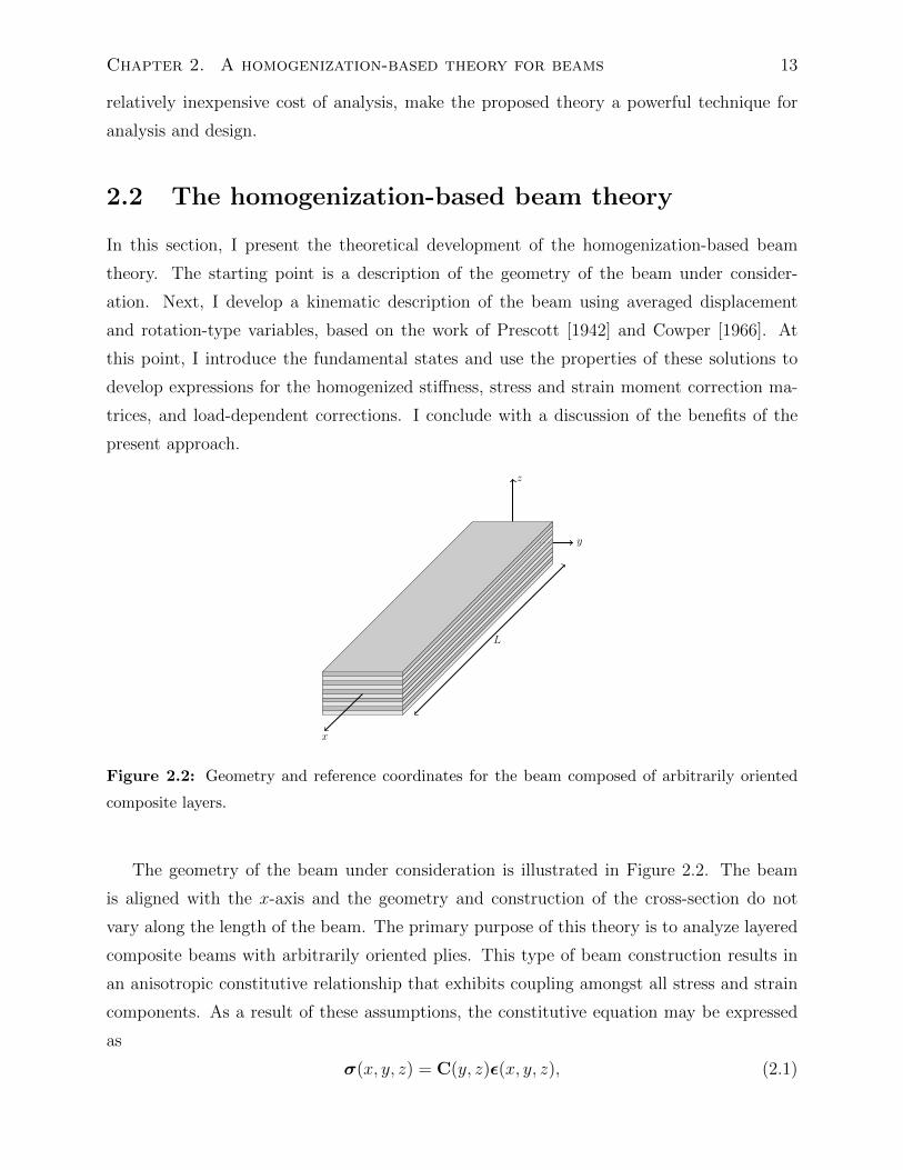
Figure 2.2: Geometry and reference coordinates for the beam composed of arbitrarily oriented
composite layers.
The geometry of the beam under consideration is illustrated in Figure 2.2. The beam
is aligned with the x-axis and the geometry and construction of the cross-section do not
vary along the length of the beam. The primary purpose of this theory is to analyze layered
composite beams with arbitrarily oriented plies. This type of beam construction results in
an anisotropic constitutive relationship that exhibits coupling amongst all stress and strain
components. As a result of these assumptions, the constitutive equation may be expressed
as
σ(x, y, z) = C(y, z)ε(x, y, z), (2.1)
Chapter 2. A homogenization-based theory for beams 14
where σ(x, y, z) and ε(x, y, z) are the full states of stress and strain, and C(y, z) is the
constitutive relationship.
The beam of length L is subject to distributed surface tractions applied in the plane
perpendicular to the x-axis and is subject to axial forces, bending moments, shear forces
and torques at its ends. Shearing tractions applied on the surface of the beam in the x
direction are excluded from consideration.
The reference axis is located at the geometric centroid of the section and the coordinate
axes are aligned with the principal axes of the section. As a result, the moments of area are
defined as follows:
A =
∫Ω
dΩ, Iz =
∫Ω
z2 dΩ, Iy =
∫Ω
y2 dΩ,∫Ω
y dΩ = 0,
∫Ω
z dΩ = 0,
∫Ω
yz dΩ = 0.
The restriction to principal coordinate axes simplifies many of the expressions that are
required below.
2.2.1 The displacement representation
Following the work of Prescott [1942] and Cowper [1966], the exact displacement field can
be expressed in terms of an average representation of the displacement field and residual
displacements. The residual displacements capture the part of the displacement field that
deviates from the average representation. This decomposition of the displacement field is
expressed as
u(x, y, z) =
u(x, y, z)
v(x, y, z)
w(x, y, z)
=
u0(x) + zuz(x) + yuy(x) + u(x, y, z)
v0(x)− zθ(x) + v(x, y, z)
w0(x) + yθ(x) + w(x, y, z)
, (2.2)
where u(x, y, z), and u(x, y, z) =[u v w
]Tare the displacements and residual displace-
ments, respectively. The x-component of the residual displacement u(x, y, z) represents the
warping of the section in the axial direction. For convenience, I collect the variables, u0, v0,
θ, uz and uy in a vector u0(x), defined as follows:
u0(x) =[u0 v0 w0 θ uz uy
]T=
∫Ω
[u
A
v
A
w
A
(yw − zv)
Iy + Iz
zu
Iz
yu
Iy
]TdΩ
= L0u(x, y, z).
(2.3)
Chapter 2. A homogenization-based theory for beams 15
Here, u0, v0, and w0 are average displacements in the x, y and z directions. The terms uz,
uy and θ are normalized first-order displacement moments about the z, y and x directions,
respectively. Note that uz, uy and θ represent rotation-type variables, but are not equal to
the average rotations of the section. The vector of variables u0(x) are called the normal-
ized displacement moments, since these variables represent zeroth and first-order normalized
moments of the displacement field u(x, y, z). In addition, the operator L0 is introduced in
Equation (2.3). This operator takes the full three-dimensional displacement field, u(x, y, z),
and returns the normalized moments of displacement. Note that the action of L0 removes
the y-z dependence of the displacement field.
At this point it should be emphasized that the displacement field decomposition (2.2)
ensures that the normalized displacement moments of the residual displacement field are
identically zero, i.e.,
L0u(x, y, z) = 0.
This property of the residual displacement field will be required later to simplify expressions
for the strain moments.
The strain produced by the displacements (2.2) is:
ε(x, y, z) =
εx
εy
εz
γyz
γxz
γxy
=
u0,x + yuy,x + zuz,z + u,x
v,y
w,z
v,z + w,y
uz + w0,x + yθ,x + u,z + w,x
uy + v0,x − zθ,x + u,y + v,x
, (2.4)
where the comma convention has been used to denote differentiation. Note that the exact
pointwise strain distribution requires knowledge of the residual displacements u(x, y, z).
Instead of using pointwise-strain directly, the homogenization-based approach uses mo-
ments of the strain across the section of the beam. This choice has the advantage that
the strain moments are defined regardless of the through-thickness behavior of the pointwise
strain. This property is important since some pointwise strain components are discontinuous
at material interfaces. It is important to recognize, however, that these interfaces are always
parallel to the x direction. As a result, differentiation with respect to x can commute with
integration across the section in the regular manner.
Chapter 2. A homogenization-based theory for beams 16
The strain moments are defined as follows:
e(x) =[ex κz κy et exz exy
]T=
∫Ω
[εx zεx yεx (yγxz − zγxy) γxz γxy
]TdΩ
= Lsε(x, y, z).
(2.5)
Here another operator Ls is introduced that takes the full strain field ε(x, y, z) and returns
the moments of strain e(x).
The next step in the development of the theory is to express the strain moments in terms
of the displacement representation (2.2). Using the strain-displacement relationships (2.4),
the definitions of the displacement moments (2.3), and the moments of area, the strain
moments can be written as follows:
e(x) =
Au0,x
Izuz,x
Iyuy,x
(Iy + Iz) θ,x
A (uz + w0,x)
A (uy + v0,x)
+ e(x) = ALεu0(x) + e(x), (2.6)
where e(x) are the moments of the strain produced by the residual displacement. Here A is
a diagonal matrix given by
A = diag A, Iz, Iy, (Iy + Iz), A,A .
The operator Lε takes the vector of average displacements and normalized displacement
moments u0(x), such that ALεu0 produces the first term on the right hand side of Equa-
tion (2.6). Note that action of the operator Lε on the normalized displacements, Lεu0(x), pro-
duces terms that are identical in form to the center-line strain used in classical Timoshenko
beam theory. However, here the variables u0(x) are interpreted as normalized displacement
moments taken from Equation (2.3), not as center-line displacements and rotations.
The term e(x) in the strain moment expression (2.6), is a function of the axial residual
Chapter 2. A homogenization-based theory for beams 17
displacement u(x, y, z) and is defined as follows:
e(x) =
∫Ω
u,x
zu,x
yu,x
y (u,z + w,x)− z (u,y + v,x)
u,z + w,x
u,y + v,x
dΩ =
∫Ω
0
0
0
yu,z − zu,yu,z
u,y
dΩ
= Lu(x, y, z),
(2.7)
where the relationship L0u = 0 is used to simplify the expression on the right-hand side
of the above equation. An additional linear operator L has been introduced that takes the
residual axial displacement u(x, y, z) and returns the moments e(x).
The strain moments corresponding to torsion et and shear exz and exy involve terms from
both the normalized displacement moments and the residual axial displacement, u(x, y, z).
These extra terms cannot be evaluated unless u(x, y, z) is known. The approach taken below
is to account for the effect of the residual displacements while formulating the theory in
terms of the average displacement variables, u0(x).
2.2.2 The equilibrium equations
The equilibrium equations are formulated based on the classical approach of integrating
moments of the three-dimensional equilibrium equations over the cross-section of the beam.
The axial, bending, torsion and shear resultants are defined as follows,
s(x) =[N Mz My T Qz Qy
]T=
∫Ω
[σx zσx yσx (yσxz − zσxy) σxz σxy
]TdΩ
= Lsσ(x, y, z).
(2.8)
Here, Ls is the same operator that was introduced for the strain moments (2.5). The vari-
ables s(x) are the stress resultants or stress moments. Integrating the three-dimensional
Chapter 2. A homogenization-based theory for beams 18
equilibrium equations over the section results in the following equilibrium equations:
N,x
My,x −Qz
Mz,x −Qy
T,x
Qy,x
Qz,x
+
0
0
0
Px
Py
Pz
= 0. (2.9)
The torque Px(x) and forces Py(x) and Pz(x) are defined as follows:
Px(x) =
∫S
ytz − zty dS,
Py(x) =
∫S
ty dS,
Pz(x) =
∫S
tz dS,
(2.10)
where ty and tz are the y and z components of the surface traction. The integrals above are
carried out over the boundary of the cross-section S.
2.2.3 The fundamental states
In this section, I present a decomposition of the stress and strain distribution within the
beam. This stress and strain decomposition is based on a linear combination of axially-
invariant stress and strain solutions called the fundamental states. The use of the fundamen-
tal states leads to a consistent method for deriving the constitutive relationship between the
stress resultants and the strain moments. Furthermore, the fundamental states can be used to
reconstruct the approximate stress and strain distribution in the beam in a post-processing
step. This representation of the solution is similar to the stress representation presented
by Ladeveze and Simmonds [1998] and used by El Fatmi [2007a,b]. Unlike these authors
however, I also use an analogous representation of the strain solution that is later used to
construct the homogenized stiffness relationship. In this section I describe the properties of
the fundamental states and how they are used in the present theory.
The fundamental states are the axially-invariant, or x-independent, stress and strain
solutions. These solutions are obtained from specially-chosen, statically determinate beam
problems. The loading conditions leading to the fundamental states are shown in Figure 2.3.
These beam problems are sometimes referred to as the Saint–Venant problem [Iesan, 1986a],
for axial, bending, torsion, and shear loads, and the Almansi–Michell problem [Iesan, 1986b],
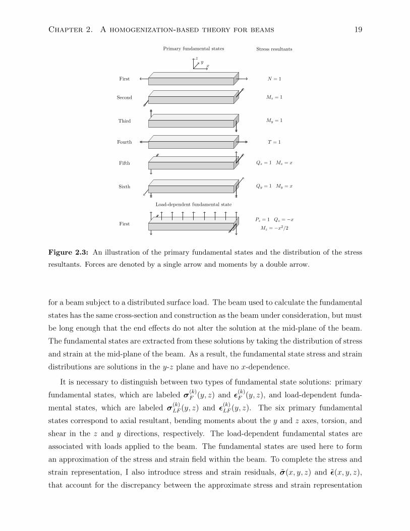
Chapter 2. A homogenization-based theory for beams 19
Primary fundamental states Stress resultants
xy
z
First N = 1
Second Mz = 1
Third My = 1
Fourth T = 1
Fifth Qz = 1 Mz = x
Sixth Qy = 1 My = x
Load-dependent fundamental state
FirstPz = 1 Qz = −x
Mz = −x2/2
Figure 2.3: An illustration of the primary fundamental states and the distribution of the stress
resultants. Forces are denoted by a single arrow and moments by a double arrow.
for a beam subject to a distributed surface load. The beam used to calculate the fundamental
states has the same cross-section and construction as the beam under consideration, but must
be long enough that the end effects do not alter the solution at the mid-plane of the beam.
The fundamental states are extracted from these solutions by taking the distribution of stress
and strain at the mid-plane of the beam. As a result, the fundamental state stress and strain
distributions are solutions in the y-z plane and have no x-dependence.
It is necessary to distinguish between two types of fundamental state solutions: primary
fundamental states, which are labeled σ(k)F (y, z) and ε
(k)F (y, z), and load-dependent funda-
mental states, which are labeled σ(k)LF (y, z) and ε
(k)LF (y, z). The six primary fundamental
states correspond to axial resultant, bending moments about the y and z axes, torsion, and
shear in the z and y directions, respectively. The load-dependent fundamental states are
associated with loads applied to the beam. The fundamental states are used here to form
an approximation of the stress and strain field within the beam. To complete the stress and
strain representation, I also introduce stress and strain residuals, σ(x, y, z) and ε(x, y, z),
that account for the discrepancy between the approximate stress and strain representation
Chapter 2. A homogenization-based theory for beams 20
and the exact distribution.
Using these definitions, the stress and strain in the beam may be expressed as follows:
σ(x, y, z) =6∑
k=1
sk(x)σ(k)F (y, z) +
N∑k=1
Pk(x)σ(k)FL(y, z) + σ(x, y, z), (2.11a)
ε(x, y, z) =6∑
k=1
sk(x)ε(k)F (y, z) +
N∑k=1
Pk(x)ε(k)FL(y, z) + ε(x, y, z). (2.11b)
The magnitudes of the primary fundamental states are given by the components of the vector
s(x) and represent axial force, bending moments, torsion, and shear resultants. Individual
components of s(x) are written as sk(x). Note that the magnitudes of the load-dependent
fundamental states Pk(x) are known from the loading conditions and that the fundamental
state magnitudes link the stress and strain distribution.
For consistency between the stress resultants and the stress distribution, the primary
fundamental states must satisfy the relationship,
Lsσ(k)F (y, z) = ik, k = 1, . . . , 6, (2.12)
where ik is the kth Cartesian basis vector. This relationship ensures that the stress resul-
tants of the stress distribution (2.11a) are equal to sk(x). Furthermore, the load-dependent
fundamental states must satisfy
Lsσ(k)FL(y, z) = 0, k = 1, . . . , N. (2.13)
The load-dependent fundamental states do not contribute to the stress resultants. In addi-
tion, the stress moments of the stress residuals must be zero, i.e.,
Lsσ(x, y, z) = 0.
An important benefit of the stress and strain distributions (2.11) is that they can capture
all components of stress and strain. Typically, beam theories retain only a few components
of the stress and strain and assume that the remaining components are negligible. These
neglected components can sometimes be determined using a post-processing integration of
the equilibrium equations through the thickness. For composite materials, however, it can
be important to retain all components of stress and strain, since singularities can arise at
ply interfaces and both strength and stiffness vary significantly between different material
directions [Pagano and Pipes, 1971].
Chapter 2. A homogenization-based theory for beams 21
2.2.4 The constitutive relationship
With these definitions, it is now possible to derive the relationship between the stress resul-
tants and the strain moments. The starting point for the derivation is the expression for the
strain field (2.11b). Using the moment operator Ls, the strain moments of Equation (2.11b)
become,
e(x) =6∑
k=1
sk(x)Lsε(k)F (y, z) +
N∑k=1
Pk(x)Lsε(k)FL(y, z) + Lsε(x, y, z). (2.14)
Note that the strain moments have contributions from all fundamental states and the strain
residuals.
Next, I introduce a square flexibility matrix E whose kth column contains the strain
moments from the kth primary fundamental state. The components of the matrix E are:
E∗k = Lsε(k)F (y, z), k = 1, . . . , 6, (2.15)
where E∗k is the kth column of the matrix E. Note that the matrix E is constant for a given
beam construction and is independent of x.
The contributions to the strain moments from the primary fundamental states are the
product of the matrix E and the primary fundamental state magnitudes s(x). Rearranging
the strain moment relationship (2.14) and using the flexibility matrix E yields
Es(x) = e(x)−N∑k=1
Pk(x)Lsε(k)FL(y, z)− Lsε(x, y, z). (2.16)
The stiffness form of the constitutive relationship can be found by inverting the matrix of
strain moments D = E−1, to obtain
s(x) = D
(e(x)−
N∑k=1
Pk(x)Lsε(k)FL(y, z)− Lsε(x, y, z)
). (2.17)
For a section composed of a single isotropic material the relationship between stress and
strain moments simplifies to
D = diag E,E,E,G,G,G .
Equation (2.17) is exact in the sense that the stress moments can be determined exactly if
the strain moments, load-dependent strain moments and strain residuals ε(x, y, z) are known.
Unfortunately, evaluating the strain residuals ε(x, y, z) requires a full three-dimensional so-
lution of the equations of elasticity.
Chapter 2. A homogenization-based theory for beams 22
At this point, an assumption must be made about the contribution to the strain moments
from the term Lsε. Since three-dimensional solutions are typically not available, I assume
that the contribution from term Lsε is small and can thus be neglected. This assumption
introduces an error in the predicted strain moments, and as a result, also introduces an
error in the predicted stress resultants. Typically, the magnitude of Lsε is highest near the
ends of the beam where the solution must adjust to satisfy the end conditions. In situations
where these disturbed regions require precise modeling, a beam theory is not appropriate.
However, at a sufficient distance from the ends of the beam, the strain representation (2.11b)
is accurate and thus Lsε should be small.
2.2.5 The stress and strain moment corrections
Next, a relationship between strain moments and the normalized displacement moments is
required. Initially, I limit the analysis to conditions where no external loads are applied to
the beam. Starting from the stiffness form of the constitutive equations (2.17), and assuming
that the strain residual moments are negligible Lsε = 0, the stress moments may be expressed
in terms of the normalized displacement moments u0(x) and the moments of the warping
strain e(x) using Equation (2.6),
s(x) = D (ALεu0(x) + e(x)) . (2.18)
To proceed, an expression for e(x) must be obtained. Following the arguments presented
by Cowper [1966], this term should be linearly dependent on the magnitudes of the primary
fundamental states in regions sufficiently far removed from end effects or rapidly varying
loads. This dependence can be written as
e(x) = Es(x) + er, (2.19)
where E is a flexibility matrix defined below. Here er, is a warping residual term that
accounts for the deviation of the warping moment in disturbed regions of the beam, called
the strain correction error.
Using the operator L from Equation (2.7), the matrix E can be written as
E∗k = Lu(k)F (y, z), k = 1, . . . , 6, (2.20)
where u(k)F (y, z) is determined from the residual displacement of the kth primary fundamental
state. Note that due to the nature of the operator L, the matrix E only has entries in the
last three rows. All other entries in E are zero.
Chapter 2. A homogenization-based theory for beams 23
An expression for the stress resultants in terms of the normalized displacement moments
can be obtained by using the simplified form of the constitutive relationship (2.18), and the
moments of the strain due to warping (2.19), yielding
s(x) = (E− E)−1ALεu0(x) + (E− E)−1er. (2.21)
In the remainder of this section I assume that the strain correction error is negligible, i.e.,
er = 0.
In order to isolate the effect of the terms E, the strain moment correction matrix may
be introduced as follows:
Cs = (I− ED)−1, (2.22)
such that Equation (2.21), with er = 0, simplifies to
s(x) = DCsALεu0(x).
Here, the strain moment correction matrix (2.22) provides a correction to the strain mo-
ments predicted from the average displacements that accounts for e(x). Note that the strain
moment correction matrix Cs has a specific structure. The first three rows of Cs are always
equal to the identity matrix, while the last three rows may contain non-zeros in any location
due to the definition of the matrix E.
A stress moment correction matrix may also be defined as follows:
Ks = (I−DE)−1, (2.23)
such that Equation (2.21), with er = 0, simplifies to
s(x) = KsDALεu0(x).
The stress moment correction matrix (2.23) provides a correction to the stress moments that
accounts for e(x). In general, the stress moment correction matrix Ks is fully populated.
In the case of a doubly symmetric, isotropic section, the stress and strain corrections
matrices are diagonal and equal. In this case, Cs and Ks take the form
Ks = Cs = diag1, 1, 1, kt, kxz, kxy,
where kt = J/(Iy + Iz) is the strain correction associated with torsion, and J is the torsional
rigidity of the section. The shear strain correction factors kxz and kxy are identical to those
Chapter 2. A homogenization-based theory for beams 24
obtained by Cowper [1966] and Mason and Herrmann [1968],
kxz =2(1 + ν)Iz
ν
2(Iy − Iz)−
A
Iz
∫Ω
z2y2 + zχz dΩ
kxy =2(1 + ν)Iy
ν
2(Iz − Iy)−
A
Iy
∫Ω
z2y2 + yχy dΩ
where χz and χy are classical Saint–Venant flexure functions [Love, 1920].
2.2.6 The load-dependent corrections
The constitutive relationship (2.21) derived above explicitly excluded the effect of externally
applied loads. At this point, I derive load-dependent corrections that account for the effect
of external loads. Again, the starting point is the flexibility form of the constitutive equa-
tions (2.16). Neglecting the moments of the strain residuals, Lsε = 0, results in the following
expression for the strain moments:
e(x) = Es(x) +N∑k=1
Pk(x)Lsε(k)FL(y, z). (2.24)
The next step is to obtain an expression for the strain moments e(x) as a function of the
normalized displacement moments u0(x). The externally applied loads produce additional
moments of the warping strain. In an analogous manner to the primary fundamental state
contributions, I assume that these moments of the warping strain are predicted by the load-
dependent fundamental states and are proportional to the applied load. These assumptions
result in the following expression:
e(x) = ALεu0(x) + Es(x) +N∑k=1
Pk(x)Lu(k)FL(y, z) + er. (2.25)
Here, u(k)FL(y, z) denotes the warping function associated with the kth load-dependent funda-
mental state and er, is the strain correction error.
Again, assuming that er = 0, the flexibility form of the constitutive equations (2.24) and
the strain moment expression (2.25) can now be combined into a constitutive relationship
that takes the following form:
s(x) = (E− E)−1ALεu0(x) +N∑k=1
Pk(x)s(k)FL, (2.26)
Chapter 2. A homogenization-based theory for beams 25
where the load-dependent stress moment corrections s(k)FL are defined as
s(k)FL = (E− E)−1
(Lu(k)
FL(y, z)− Lsε(k)FL(y, z)
). (2.27)
In a similar fashion, it can be shown that the strain moments take the modified form
e(x) = CsALεu0 +N∑k=1
Pk(x)e(k)FL, (2.28)
where the load-dependent strain moment corrections e(k)FL are defined as
e(k)FL = Cs
(Lu(k)
FL(y, z)− Lsε(k)FL(y, z)
)+ Lsε(k)
FL(y, z). (2.29)
The load-dependent stress moment corrections (2.27) and the load-dependent strain mo-
ment corrections (2.29) take into account the change in the relationship between the stress
and strain moments and the normalized displacement moments as a result of externally ap-
plied loads. The externally applied loads do not directly produce stress moments; rather,
these loads produce strain moments that must be taken into account in the constitutive
relationship (2.26). The main assumptions required for the derivation of the constitutive
expression are that the moments of the strain residuals, Lsε, and the strain moment correc-
tion, er, can be neglected. These assumptions are examined below in the numerical results
section.
2.2.7 The asymmetry of the constitutive relationship
In general, the homogenized stiffness matrix D, and the matrix product DCsA are not sym-
metric. This is not a classical result and deserves attention. Linear constitutive relationships
between pointwise stress and pointwise strain expressed in the form of Equation (2.1) are
symmetric due to the existence of the strain energy density. However, the homogenized
stiffness matrix D that relates the stress resultants to the strain moments cannot be derived
from a strain energy density, since D relates integrated quantities. The integral of the point-
wise strain energy density across the section cannot be related directly to the product of the
integrals of stress and strain. As a result, D is not guaranteed to be symmetric. The matrix
product DCsA that relates the normalized displacement moments to the stress resultants
is not symmetric based on the same argument. Therefore, symmetry of the constitutive
relationship cannot be assumed within the context of a finite-element implementation of the
present beam theory.
Chapter 2. A homogenization-based theory for beams 26
2.3 A finite-element method for the fundamental states
The fundamental states play an important role within the beam theory presented in Sec-
tion 2.2. In principle, full three-dimensional solutions for each of the fundamental states are
required before any analysis can be performed. It is possible to derive some exact solutions to
the fundamental states. However, these exact solutions can only be obtained for a small set
of geometries and beam constructions of interest. In order to solve more general problems,
it is necessary to develop a finite-element approach to determine the fundamental states for
cross-sections of arbitrary geometry and construction.
Conventional three-dimensional finite-elements can be used to obtain the fundamental
state solutions. However, this approach is computationally expensive due to the large, three-
dimensional mesh requirements. Instead, I have developed a technique to obtain the funda-
mental states that only requires computations in the plane of the section, eliminating the
need to discretize the axial direction. This approach is possible due to the fact that the
fundamental states are far-field solutions.
In developing the following finite-element method, I follow the work of Pipes and Pagano
[1970], who used a semi-inverse approach to obtain the stress and strain distributions in a
long beam subject to an axial load. I modify the form of the assumed displacement field
proposed by Pipes and Pagano [1970], but retain the terms that account for the effects of
axial force, bending, shear, and torsion. El Fatmi and Zenzri [2002] developed a similar
technique to obtain the Saint–Venant and Almansi–Michell solutions based on the work of
Ladeveze and Simmonds [1998]. Dong et al. [2001] also developed a finite-element solution
technique for the Saint–Venant problem based on the work of Iesan [1986a].
In the following section, all variables refer to a single fundamental state calculation. Rela-
tionships with the beam theory are described explicitly in Section 2.3.2. In this finite-element
approach, I develop a displacement-based solution to the three-dimensional equations of elas-
ticity based on the following expansion of the displacement field in the axial direction:
u(x, y, z) =M∑k=1
xk
k!
(c
(k)1 + c
(k)2 z + c
(k)3 y)
+xk−1
(k − 1)!U (k)(y, z)
,
v(x, y, z) =M∑k=1
xk
k!
(c
(k)6 − c(k)
4 z − c(k)3
x
k + 1
)+
xk−1
(k − 1)!V (k)(y, z)
,
w(x, y, z) =M∑k=1
xk
k!
(c
(k)5 + c
(k)4 y − c(k)
2
x
k + 1
)+
xk−1
(k − 1)!W (k)(y, z)
,
(2.30)
where the displacements U (k)(y, z), V (k)(y, z) and W (k)(y, z) are sometimes collected in the
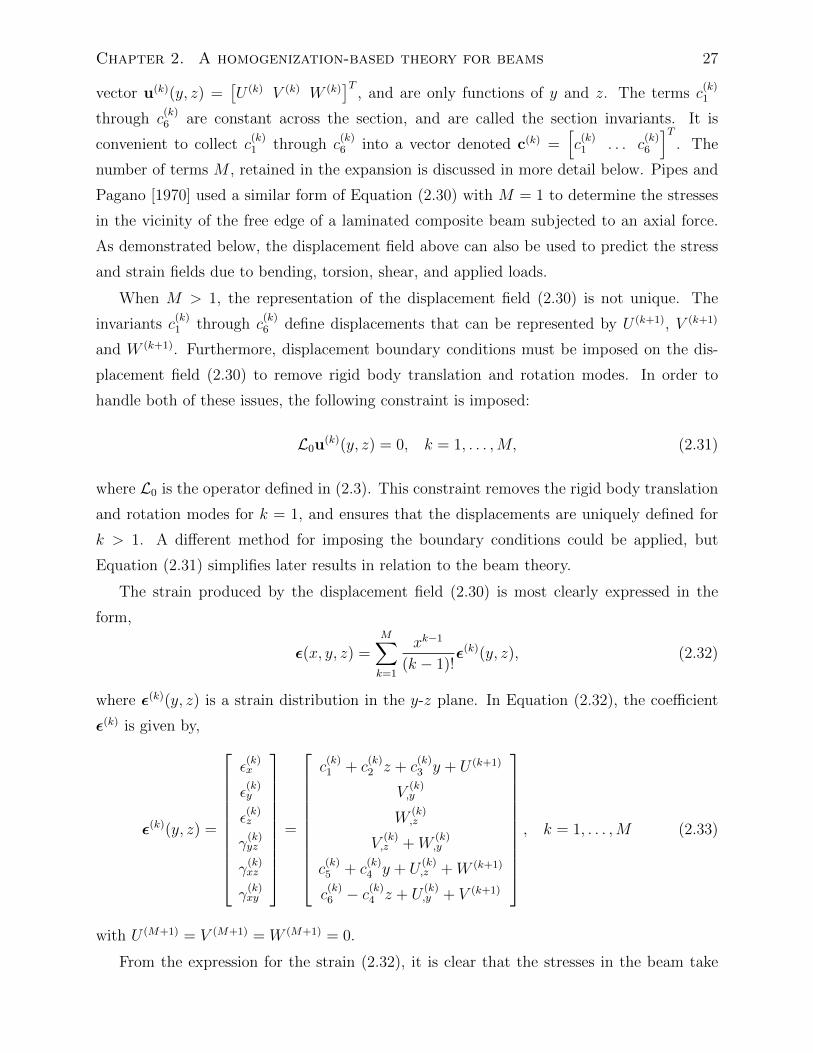
Chapter 2. A homogenization-based theory for beams 27
vector u(k)(y, z) =[U (k) V (k) W (k)
]T, and are only functions of y and z. The terms c
(k)1
through c(k)6 are constant across the section, and are called the section invariants. It is
convenient to collect c(k)1 through c
(k)6 into a vector denoted c(k) =
[c
(k)1 . . . c
(k)6
]T. The
number of terms M , retained in the expansion is discussed in more detail below. Pipes and
Pagano [1970] used a similar form of Equation (2.30) with M = 1 to determine the stresses
in the vicinity of the free edge of a laminated composite beam subjected to an axial force.
As demonstrated below, the displacement field above can also be used to predict the stress
and strain fields due to bending, torsion, shear, and applied loads.
When M > 1, the representation of the displacement field (2.30) is not unique. The
invariants c(k)1 through c
(k)6 define displacements that can be represented by U (k+1), V (k+1)
and W (k+1). Furthermore, displacement boundary conditions must be imposed on the dis-
placement field (2.30) to remove rigid body translation and rotation modes. In order to
handle both of these issues, the following constraint is imposed:
L0u(k)(y, z) = 0, k = 1, . . . ,M, (2.31)
where L0 is the operator defined in (2.3). This constraint removes the rigid body translation
and rotation modes for k = 1, and ensures that the displacements are uniquely defined for
k > 1. A different method for imposing the boundary conditions could be applied, but
Equation (2.31) simplifies later results in relation to the beam theory.
The strain produced by the displacement field (2.30) is most clearly expressed in the
form,
ε(x, y, z) =M∑k=1
xk−1
(k − 1)!ε(k)(y, z), (2.32)
where ε(k)(y, z) is a strain distribution in the y-z plane. In Equation (2.32), the coefficient
ε(k) is given by,
ε(k)(y, z) =
ε(k)x
ε(k)y
ε(k)z
γ(k)yz
γ(k)xz
γ(k)xy
=
c(k)1 + c
(k)2 z + c
(k)3 y + U (k+1)
V(k),y
W(k),z
V(k),z +W
(k),y
c(k)5 + c
(k)4 y + U
(k),z +W (k+1)
c(k)6 − c(k)
4 z + U(k),y + V (k+1)
, k = 1, . . . ,M (2.33)
with U (M+1) = V (M+1) = W (M+1) = 0.
From the expression for the strain (2.32), it is clear that the stresses in the beam take
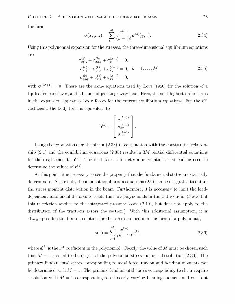
Chapter 2. A homogenization-based theory for beams 28
the form
σ(x, y, z) =M∑k=1
xk−1
(k − 1)!σ(k)(y, z). (2.34)
Using this polynomial expansion for the stresses, the three-dimensional equilibrium equations
areσ(k)xy,y + σ(k)
xz,z + σ(k+1)x = 0,
σ(k)y,y + σ(k)
yz,z + σ(k+1)xy = 0,
σ(k)yz,y + σ(k)
z,z + σ(k+1)xz = 0,
k = 1, . . . ,M (2.35)
with σ(M+1) = 0. These are the same equations used by Love [1920] for the solution of a
tip-loaded cantilever, and a beam subject to gravity load. Here, the next highest-order terms
in the expansion appear as body forces for the current equilibrium equations. For the kth
coefficient, the body force is equivalent to
b(k) =
σ
(k+1)x
σ(k+1)xy
σ(k+1)xz
.Using the expressions for the strain (2.33) in conjunction with the constitutive relation-
ship (2.1) and the equilibrium equations (2.35) results in 3M partial differential equations
for the displacements u(k). The next task is to determine equations that can be used to
determine the values of c(k).
At this point, it is necessary to use the property that the fundamental states are statically
determinate. As a result, the moment equilibrium equations (2.9) can be integrated to obtain
the stress moment distribution in the beam. Furthermore, it is necessary to limit the load-
dependent fundamental states to loads that are polynomials in the x direction. (Note that
this restriction applies to the integrated pressure loads (2.10), but does not apply to the
distribution of the tractions across the section.) With this additional assumption, it is
always possible to obtain a solution for the stress moments in the form of a polynomial,
s(x) =M∑k=1
xk−1
(k − 1)!s(k)c , (2.36)
where s(k)c is the kth coefficient in the polynomial. Clearly, the value of M must be chosen such
that M − 1 is equal to the degree of the polynomial stress-moment distribution (2.36). The
primary fundamental states corresponding to axial force, torsion and bending moments can
be determined with M = 1. The primary fundamental states corresponding to shear require
a solution with M = 2 corresponding to a linearly varying bending moment and constant
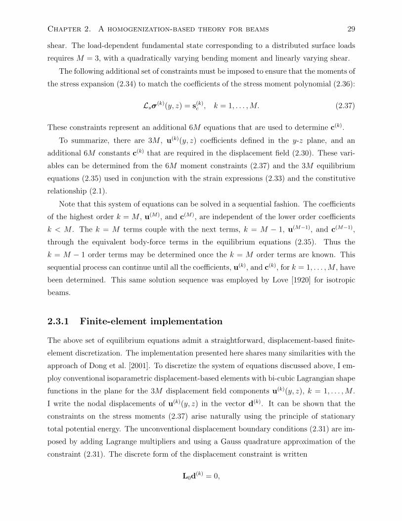
Chapter 2. A homogenization-based theory for beams 29
shear. The load-dependent fundamental state corresponding to a distributed surface loads
requires M = 3, with a quadratically varying bending moment and linearly varying shear.
The following additional set of constraints must be imposed to ensure that the moments of
the stress expansion (2.34) to match the coefficients of the stress moment polynomial (2.36):
Lsσ(k)(y, z) = s(k)c , k = 1, . . . ,M. (2.37)
These constraints represent an additional 6M equations that are used to determine c(k).
To summarize, there are 3M , u(k)(y, z) coefficients defined in the y-z plane, and an
additional 6M constants c(k) that are required in the displacement field (2.30). These vari-
ables can be determined from the 6M moment constraints (2.37) and the 3M equilibrium
equations (2.35) used in conjunction with the strain expressions (2.33) and the constitutive
relationship (2.1).
Note that this system of equations can be solved in a sequential fashion. The coefficients
of the highest order k = M , u(M), and c(M), are independent of the lower order coefficients
k < M . The k = M terms couple with the next terms, k = M − 1, u(M−1), and c(M−1),
through the equivalent body-force terms in the equilibrium equations (2.35). Thus the
k = M − 1 order terms may be determined once the k = M order terms are known. This
sequential process can continue until all the coefficients, u(k), and c(k), for k = 1, . . . ,M , have
been determined. This same solution sequence was employed by Love [1920] for isotropic
beams.
2.3.1 Finite-element implementation
The above set of equilibrium equations admit a straightforward, displacement-based finite-
element discretization. The implementation presented here shares many similarities with the
approach of Dong et al. [2001]. To discretize the system of equations discussed above, I em-
ploy conventional isoparametric displacement-based elements with bi-cubic Lagrangian shape
functions in the plane for the 3M displacement field components u(k)(y, z), k = 1, . . . ,M .
I write the nodal displacements of u(k)(y, z) in the vector d(k). It can be shown that the
constraints on the stress moments (2.37) arise naturally using the principle of stationary
total potential energy. The unconventional displacement boundary conditions (2.31) are im-
posed by adding Lagrange multipliers and using a Gauss quadrature approximation of the
constraint (2.31). The discrete form of the displacement constraint is written
L0d(k) = 0,
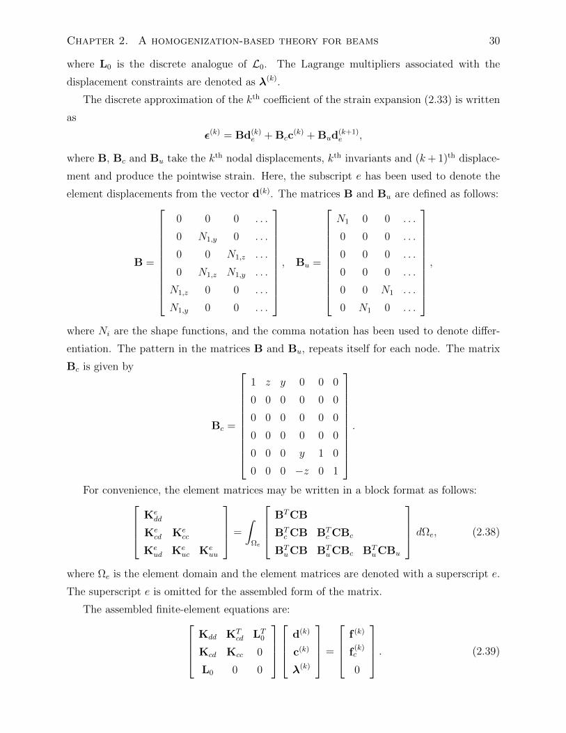
Chapter 2. A homogenization-based theory for beams 30
where L0 is the discrete analogue of L0. The Lagrange multipliers associated with the
displacement constraints are denoted as λ(k).
The discrete approximation of the kth coefficient of the strain expansion (2.33) is written
as
ε(k) = Bd(k)e + Bcc
(k) + Bud(k+1)e ,
where B, Bc and Bu take the kth nodal displacements, kth invariants and (k+ 1)th displace-
ment and produce the pointwise strain. Here, the subscript e has been used to denote the
element displacements from the vector d(k). The matrices B and Bu are defined as follows:
B =
0 0 0 . . .
0 N1,y 0 . . .
0 0 N1,z . . .
0 N1,z N1,y . . .
N1,z 0 0 . . .
N1,y 0 0 . . .
, Bu =
N1 0 0 . . .
0 0 0 . . .
0 0 0 . . .
0 0 0 . . .
0 0 N1 . . .
0 N1 0 . . .
,
where Ni are the shape functions, and the comma notation has been used to denote differ-
entiation. The pattern in the matrices B and Bu, repeats itself for each node. The matrix
Bc is given by
Bc =
1 z y 0 0 0
0 0 0 0 0 0
0 0 0 0 0 0
0 0 0 0 0 0
0 0 0 y 1 0
0 0 0 −z 0 1
.
For convenience, the element matrices may be written in a block format as follows:Kedd
Kecd Ke
cc
Keud Ke
uc Keuu
=
∫Ωe
BTCB
BTc CB BT
c CBc
BTuCB BT
uCBc BTuCBu
dΩe, (2.38)
where Ωe is the element domain and the element matrices are denoted with a superscript e.
The superscript e is omitted for the assembled form of the matrix.
The assembled finite-element equations are:Kdd KT
cd LT0
Kcd Kcc 0
L0 0 0
d(k)
c(k)
λ(k)
=
f (k)
f(k)c
0
. (2.39)
Chapter 2. A homogenization-based theory for beams 31
Care must be exercised when solving equation (2.39), since the matrix Kdd is singular. This
is due to the fact that no conventional Dirichlet boundary conditions are applied to Kdd.
However, the final row of the system of equations (2.39) imposes a constraint that removes
this singularity.
The two terms on the right hand side of Equation (2.39) are
f (k) = f (k)s + f
(k)b −KT
udd(k+1),
f (k)c = s(k)
c −KTucd
(k+1),(2.40)
where terms with superscripts greater than M are zero. The term fs is the surface traction
contribution to the right hand side and fc is the right hand side for the invariants. The force
vector, f(k)b , represents a body force associated with the (k+ 1)th fundamental state, defined
as follows:
f(k)b = Kudd
(k+1) + Kucc(k+1) + Kuud
(k+2).
Note that the left hand side of Equation (2.39) is the same for each coefficient k. Therefore,
only the right hand sides (2.40) needs to be recomputed for each subsequent solution.
2.3.2 Relation to beam theory
In this section, I outline the connection between the finite-element approach described above
and the proposed beam theory.
The computations outlined above are performed for each fundamental state. First, the
polynomial stress resultant coefficients from Equation (2.36) are determined. These polyno-
mials are summarized for each of the fundamental states in Figure 2.3. Next, the unknowns
d(k) and c(k), k = 1 . . .M , are determined using Equation (2.39). The fundamental state
stress and strain solutions are the lowest-order terms of the polynomial expressions for the
stress in Equations (2.34) and (2.32), respectively. Therefore, the fundamental states are
σ(1)(y,z) and ε(1)(y, z) in the y-z plane.
With this definition, the strain moments of the fundamental state can be computed using
e = Lsε(1)(y, z), (2.41)
where Ls is a discrete analogue of the operator Ls computed using Gaussian quadrature. The
strain moments are required to compute the flexibility matrix E (2.15) and for components
of the stress and strain moment corrections in Equations (2.27) and (2.29), respectively.
Another key quantity required for the beam theory is the axial warping u(x, y, z). The
x-independent component of axial warping is precisely U (1)(y, z) due to the imposition of
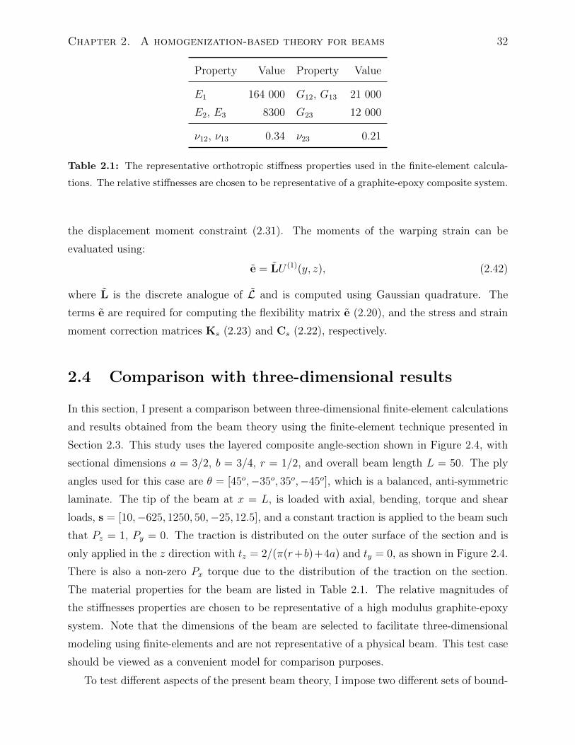
Chapter 2. A homogenization-based theory for beams 32
Property Value Property Value
E1 164 000 G12, G13 21 000
E2, E3 8300 G23 12 000
ν12, ν13 0.34 ν23 0.21
Table 2.1: The representative orthotropic stiffness properties used in the finite-element calcula-
tions. The relative stiffnesses are chosen to be representative of a graphite-epoxy composite system.
the displacement moment constraint (2.31). The moments of the warping strain can be
evaluated using:
e = LU (1)(y, z), (2.42)
where L is the discrete analogue of L and is computed using Gaussian quadrature. The
terms e are required for computing the flexibility matrix e (2.20), and the stress and strain
moment correction matrices Ks (2.23) and Cs (2.22), respectively.
2.4 Comparison with three-dimensional results
In this section, I present a comparison between three-dimensional finite-element calculations
and results obtained from the beam theory using the finite-element technique presented in
Section 2.3. This study uses the layered composite angle-section shown in Figure 2.4, with
sectional dimensions a = 3/2, b = 3/4, r = 1/2, and overall beam length L = 50. The ply
angles used for this case are θ = [45o,−35o, 35o,−45o], which is a balanced, anti-symmetric
laminate. The tip of the beam at x = L, is loaded with axial, bending, torque and shear
loads, s = [10,−625, 1250, 50,−25, 12.5], and a constant traction is applied to the beam such
that Pz = 1, Py = 0. The traction is distributed on the outer surface of the section and is
only applied in the z direction with tz = 2/(π(r+b)+4a) and ty = 0, as shown in Figure 2.4.
There is also a non-zero Px torque due to the distribution of the traction on the section.
The material properties for the beam are listed in Table 2.1. The relative magnitudes of
the stiffnesses properties are chosen to be representative of a high modulus graphite-epoxy
system. Note that the dimensions of the beam are selected to facilitate three-dimensional
modeling using finite-elements and are not representative of a physical beam. This test case
should be viewed as a convenient model for comparison purposes.
To test different aspects of the present beam theory, I impose two different sets of bound-
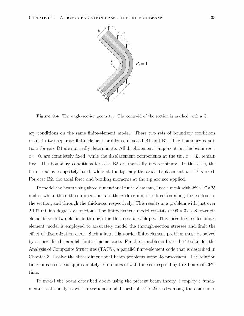
Chapter 2. A homogenization-based theory for beams 33
Cr
ba
a
Pz = 1
θ1θ2θ3θ4
Figure 2.4: The angle-section geometry. The centroid of the section is marked with a C.
ary conditions on the same finite-element model. These two sets of boundary conditions
result in two separate finite-element problems, denoted B1 and B2. The boundary condi-
tions for case B1 are statically determinate. All displacement components at the beam root,
x = 0, are completely fixed, while the displacement components at the tip, x = L, remain
free. The boundary conditions for case B2 are statically indeterminate. In this case, the
beam root is completely fixed, while at the tip only the axial displacement u = 0 is fixed.
For case B2, the axial force and bending moments at the tip are not applied.
To model the beam using three-dimensional finite-elements, I use a mesh with 289×97×25
nodes, where these three dimensions are the x-direction, the direction along the contour of
the section, and through the thickness, respectively. This results in a problem with just over
2.102 million degrees of freedom. The finite-element model consists of 96× 32× 8 tri-cubic
elements with two elements through the thickness of each ply. This large high-order finite-
element model is employed to accurately model the through-section stresses and limit the
effect of discretization error. Such a large high-order finite-element problem must be solved
by a specialized, parallel, finite-element code. For these problems I use the Toolkit for the
Analysis of Composite Structures (TACS), a parallel finite-element code that is described in
Chapter 3. I solve the three-dimensional beam problems using 48 processors. The solution
time for each case is approximately 10 minutes of wall time corresponding to 8 hours of CPU
time.
To model the beam described above using the present beam theory, I employ a funda-
mental state analysis with a sectional nodal mesh of 97 × 25 nodes along the contour of
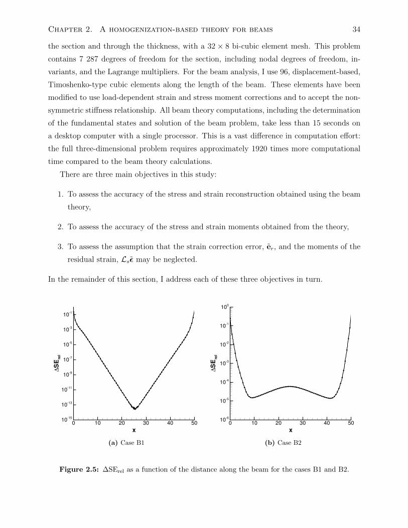
Chapter 2. A homogenization-based theory for beams 34
the section and through the thickness, with a 32 × 8 bi-cubic element mesh. This problem
contains 7 287 degrees of freedom for the section, including nodal degrees of freedom, in-
variants, and the Lagrange multipliers. For the beam analysis, I use 96, displacement-based,
Timoshenko-type cubic elements along the length of the beam. These elements have been
modified to use load-dependent strain and stress moment corrections and to accept the non-
symmetric stiffness relationship. All beam theory computations, including the determination
of the fundamental states and solution of the beam problem, take less than 15 seconds on
a desktop computer with a single processor. This is a vast difference in computation effort:
the full three-dimensional problem requires approximately 1920 times more computational
time compared to the beam theory calculations.
There are three main objectives in this study:
1. To assess the accuracy of the stress and strain reconstruction obtained using the beam
theory,
2. To assess the accuracy of the stress and strain moments obtained from the theory,
3. To assess the assumption that the strain correction error, er, and the moments of the
residual strain, Lsε may be neglected.
In the remainder of this section, I address each of these three objectives in turn.
x
∆SE
rel
0 10 20 30 40 5010
15
1013
1011
109
107
105
103
101
(a) Case B1
x
∆SE
rel
0 10 20 30 40 5010
6
105
104
103
102
101
100
(b) Case B2
Figure 2.5: ∆SErel as a function of the distance along the beam for the cases B1 and B2.
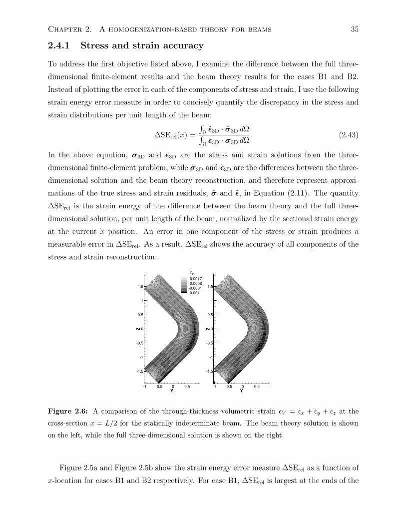
Chapter 2. A homogenization-based theory for beams 35
2.4.1 Stress and strain accuracy
To address the first objective listed above, I examine the difference between the full three-
dimensional finite-element results and the beam theory results for the cases B1 and B2.
Instead of plotting the error in each of the components of stress and strain, I use the following
strain energy error measure in order to concisely quantify the discrepancy in the stress and
strain distributions per unit length of the beam:
∆SErel(x) =
∫Ωε3D · σ3D dΩ∫
Ωε3D · σ3D dΩ
. (2.43)
In the above equation, σ3D and ε3D are the stress and strain solutions from the three-
dimensional finite-element problem, while σ3D and ε3D are the differences between the three-
dimensional solution and the beam theory reconstruction, and therefore represent approxi-
mations of the true stress and strain residuals, σ and ε, in Equation (2.11). The quantity
∆SErel is the strain energy of the difference between the beam theory and the full three-
dimensional solution, per unit length of the beam, normalized by the sectional strain energy
at the current x position. An error in one component of the stress or strain produces a
measurable error in ∆SErel. As a result, ∆SErel shows the accuracy of all components of the
stress and strain reconstruction.
Y
Z
1 0.5 0 0.5
1.5
1
0.5
0
0.5
1
1.5
Y
Z
1 0.5 0 0.5
1.5
1
0.5
0
0.5
1
1.5
0.0017
0.0008
0.0001
0.001
εV
Figure 2.6: A comparison of the through-thickness volumetric strain εV = εx + εy + εz at the
cross-section x = L/2 for the statically indeterminate beam. The beam theory solution is shown
on the left, while the full three-dimensional solution is shown on the right.
Figure 2.5a and Figure 2.5b show the strain energy error measure ∆SErel as a function of
x-location for cases B1 and B2 respectively. For case B1, ∆SErel is largest at the ends of the
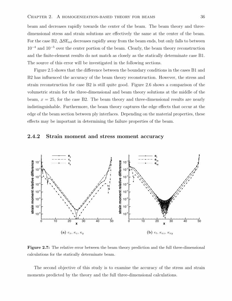
Chapter 2. A homogenization-based theory for beams 36
beam and decreases rapidly towards the center of the beam. The beam theory and three-
dimensional stress and strain solutions are effectively the same at the center of the beam.
For the case B2, ∆SErel decreases rapidly away from the beam ends, but only falls to between
10−4 and 10−5 over the center portion of the beam. Clearly, the beam theory reconstruction
and the finite-element results do not match as closely as the statically determinate case B1.
The source of this error will be investigated in the following sections.
Figure 2.5 shows that the difference between the boundary conditions in the cases B1 and
B2 has influenced the accuracy of the beam theory reconstruction. However, the stress and
strain reconstruction for case B2 is still quite good. Figure 2.6 shows a comparison of the
volumetric strain for the three-dimensional and beam theory solutions at the middle of the
beam, x = 25, for the case B2. The beam theory and three-dimensional results are nearly
indistinguishable. Furthermore, the beam theory captures the edge effects that occur at the
edge of the beam section between ply interfaces. Depending on the material properties, these
effects may be important in determining the failure properties of the beam.
2.4.2 Strain moment and stress moment accuracy
x
strain
momentrelativedifference
0 10 20 30 40 50
108
107
106
105
104
103
102
101
ex
κz
κy
(a) ex, κz, κy
x
strain
momentrelativedifference
0 10 20 30 40 50
108
107
106
105
104
103
102
101
et
exz
exy
(b) et, κxz, κxy
Figure 2.7: The relative error between the beam theory prediction and the full three-dimensional
calculations for the statically determinate beam.
The second objective of this study is to examine the accuracy of the stress and strain
moments predicted by the theory and the full three-dimensional calculations.
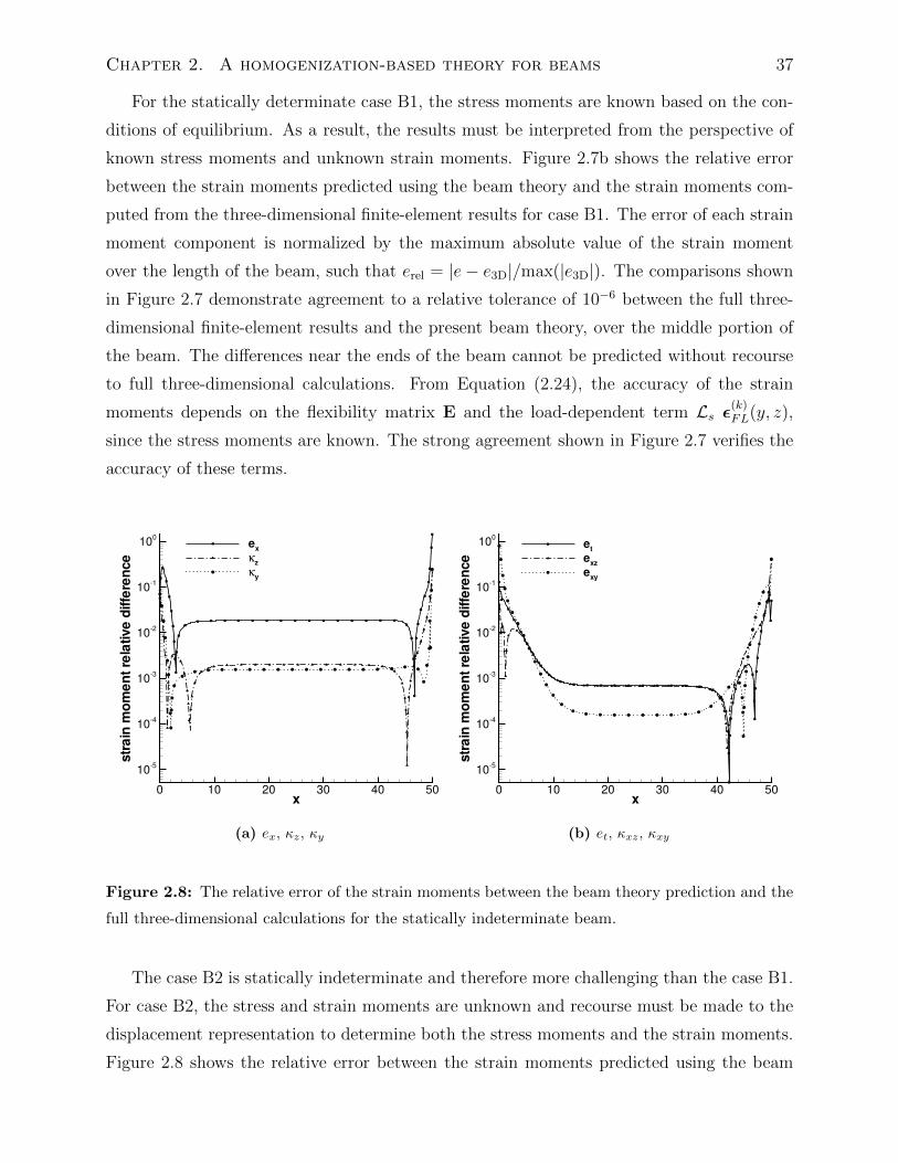
Chapter 2. A homogenization-based theory for beams 37
For the statically determinate case B1, the stress moments are known based on the con-
ditions of equilibrium. As a result, the results must be interpreted from the perspective of
known stress moments and unknown strain moments. Figure 2.7b shows the relative error
between the strain moments predicted using the beam theory and the strain moments com-
puted from the three-dimensional finite-element results for case B1. The error of each strain
moment component is normalized by the maximum absolute value of the strain moment
over the length of the beam, such that erel = |e− e3D|/max(|e3D|). The comparisons shown
in Figure 2.7 demonstrate agreement to a relative tolerance of 10−6 between the full three-
dimensional finite-element results and the present beam theory, over the middle portion of
the beam. The differences near the ends of the beam cannot be predicted without recourse
to full three-dimensional calculations. From Equation (2.24), the accuracy of the strain
moments depends on the flexibility matrix E and the load-dependent term Ls ε(k)FL(y, z),
since the stress moments are known. The strong agreement shown in Figure 2.7 verifies the
accuracy of these terms.
x
strain
momentrelativedifference
0 10 20 30 40 50
105
104
103
102
101
100
ex
κz
κy
(a) ex, κz, κy
x
strain
momentrelativedifference
0 10 20 30 40 50
105
104
103
102
101
100
et
exz
exy
(b) et, κxz, κxy
Figure 2.8: The relative error of the strain moments between the beam theory prediction and the
full three-dimensional calculations for the statically indeterminate beam.
The case B2 is statically indeterminate and therefore more challenging than the case B1.
For case B2, the stress and strain moments are unknown and recourse must be made to the
displacement representation to determine both the stress moments and the strain moments.
Figure 2.8 shows the relative error between the strain moments predicted using the beam
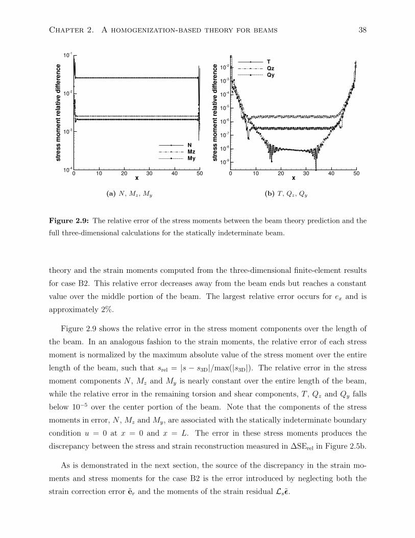
Chapter 2. A homogenization-based theory for beams 38
x
stressmomentrelativedifference
0 10 20 30 40 5010
4
103
102
101
N
Mz
My
(a) N , Mz, My
x
stressmomentrelativedifference
0 10 20 30 40 50
109
108
107
106
105
104
103
102
T
QzQy
(b) T , Qz, Qy
Figure 2.9: The relative error of the stress moments between the beam theory prediction and the
full three-dimensional calculations for the statically indeterminate beam.
theory and the strain moments computed from the three-dimensional finite-element results
for case B2. This relative error decreases away from the beam ends but reaches a constant
value over the middle portion of the beam. The largest relative error occurs for ex and is
approximately 2%.
Figure 2.9 shows the relative error in the stress moment components over the length of
the beam. In an analogous fashion to the strain moments, the relative error of each stress
moment is normalized by the maximum absolute value of the stress moment over the entire
length of the beam, such that srel = |s − s3D|/max(|s3D|). The relative error in the stress
moment components N , Mz and My is nearly constant over the entire length of the beam,
while the relative error in the remaining torsion and shear components, T , Qz and Qy falls
below 10−5 over the center portion of the beam. Note that the components of the stress
moments in error, N , Mz and My, are associated with the statically indeterminate boundary
condition u = 0 at x = 0 and x = L. The error in these stress moments produces the
discrepancy between the stress and strain reconstruction measured in ∆SErel in Figure 2.5b.
As is demonstrated in the next section, the source of the discrepancy in the strain mo-
ments and stress moments for the case B2 is the error introduced by neglecting both the
strain correction error er and the moments of the strain residual Lsε.
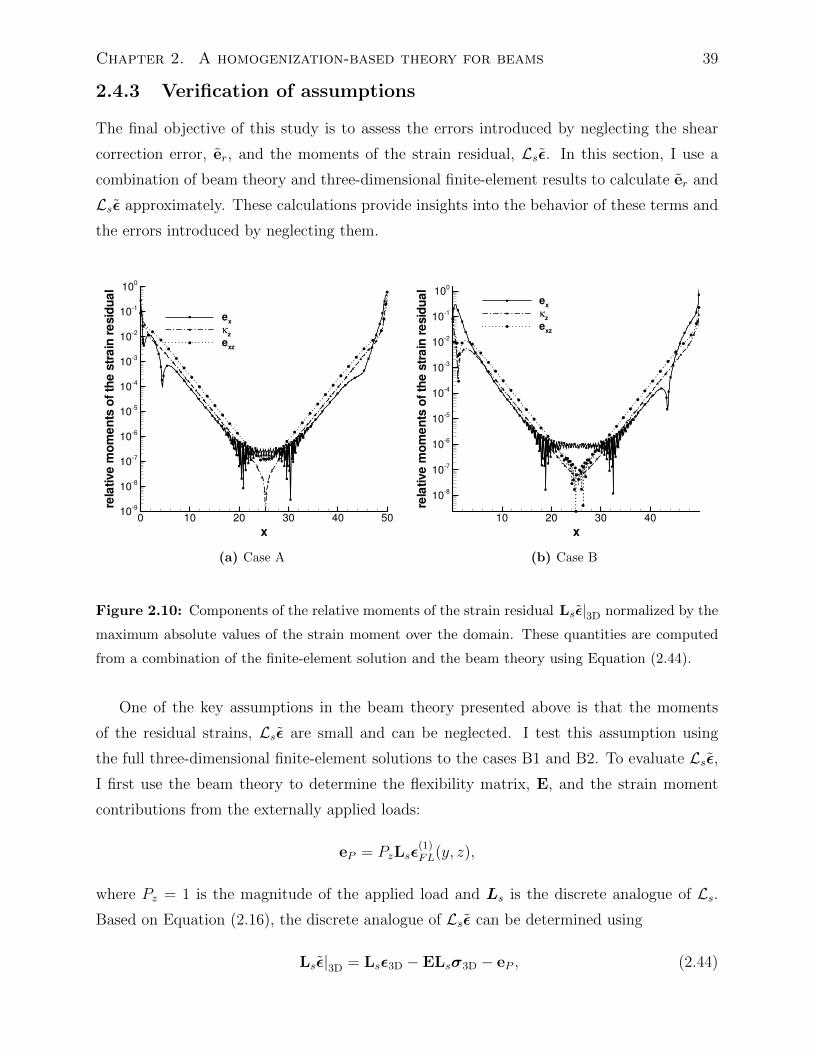
Chapter 2. A homogenization-based theory for beams 39
2.4.3 Verification of assumptions
The final objective of this study is to assess the errors introduced by neglecting the shear
correction error, er, and the moments of the strain residual, Lsε. In this section, I use a
combination of beam theory and three-dimensional finite-element results to calculate er and
Lsε approximately. These calculations provide insights into the behavior of these terms and
the errors introduced by neglecting them.
x
relativemoments
ofthestrain
residual
0 10 20 30 40 5010
9
108
107
106
105
104
103
102
101
100
ex
κz
exz
(a) Case A
x
relativemoments
ofthestrain
residual
10 20 30 40
108
107
106
105
104
103
102
101
100
ex
κz
exz
(b) Case B
Figure 2.10: Components of the relative moments of the strain residual Lsε|3D normalized by the
maximum absolute values of the strain moment over the domain. These quantities are computed
from a combination of the finite-element solution and the beam theory using Equation (2.44).
One of the key assumptions in the beam theory presented above is that the moments
of the residual strains, Lsε are small and can be neglected. I test this assumption using
the full three-dimensional finite-element solutions to the cases B1 and B2. To evaluate Lsε,I first use the beam theory to determine the flexibility matrix, E, and the strain moment
contributions from the externally applied loads:
eP = PzLsε(1)FL(y, z),
where Pz = 1 is the magnitude of the applied load and Ls is the discrete analogue of Ls.Based on Equation (2.16), the discrete analogue of Lsε can be determined using
Lsε|3D = Lsε3D − ELsσ3D − eP , (2.44)
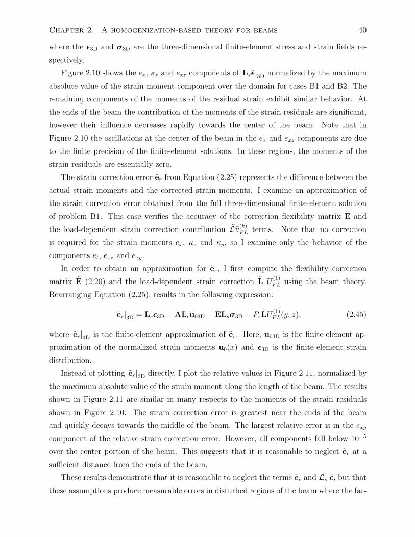
Chapter 2. A homogenization-based theory for beams 40
where the ε3D and σ3D are the three-dimensional finite-element stress and strain fields re-
spectively.
Figure 2.10 shows the ex, κz and exz components of Lsε|3D normalized by the maximum
absolute value of the strain moment component over the domain for cases B1 and B2. The
remaining components of the moments of the residual strain exhibit similar behavior. At
the ends of the beam the contribution of the moments of the strain residuals are significant,
however their influence decreases rapidly towards the center of the beam. Note that in
Figure 2.10 the oscillations at the center of the beam in the ex and exz components are due
to the finite precision of the finite-element solutions. In these regions, the moments of the
strain residuals are essentially zero.
The strain correction error er from Equation (2.25) represents the difference between the
actual strain moments and the corrected strain moments. I examine an approximation of
the strain correction error obtained from the full three-dimensional finite-element solution
of problem B1. This case verifies the accuracy of the correction flexibility matrix E and
the load-dependent strain correction contribution Lu(k)FL terms. Note that no correction
is required for the strain moments ex, κz and κy, so I examine only the behavior of the
components et, exz and exy.
In order to obtain an approximation for er, I first compute the flexibility correction
matrix E (2.20) and the load-dependent strain correction L U(1)FL using the beam theory.
Rearranging Equation (2.25), results in the following expression:
er|3D = Lsε3D −ALεu03D − ELsσ3D − PzLU (1)FL(y, z), (2.45)
where er|3D is the finite-element approximation of er. Here, u03D is the finite-element ap-
proximation of the normalized strain moments u0(x) and ε3D is the finite-element strain
distribution.
Instead of plotting er|3D directly, I plot the relative values in Figure 2.11, normalized by
the maximum absolute value of the strain moment along the length of the beam. The results
shown in Figure 2.11 are similar in many respects to the moments of the strain residuals
shown in Figure 2.10. The strain correction error is greatest near the ends of the beam
and quickly decays towards the middle of the beam. The largest relative error is in the exy
component of the relative strain correction error. However, all components fall below 10−5
over the center portion of the beam. This suggests that it is reasonable to neglect er at a
sufficient distance from the ends of the beam.
These results demonstrate that it is reasonable to neglect the terms er and Ls ε, but that
these assumptions produce measurable errors in disturbed regions of the beam where the far-
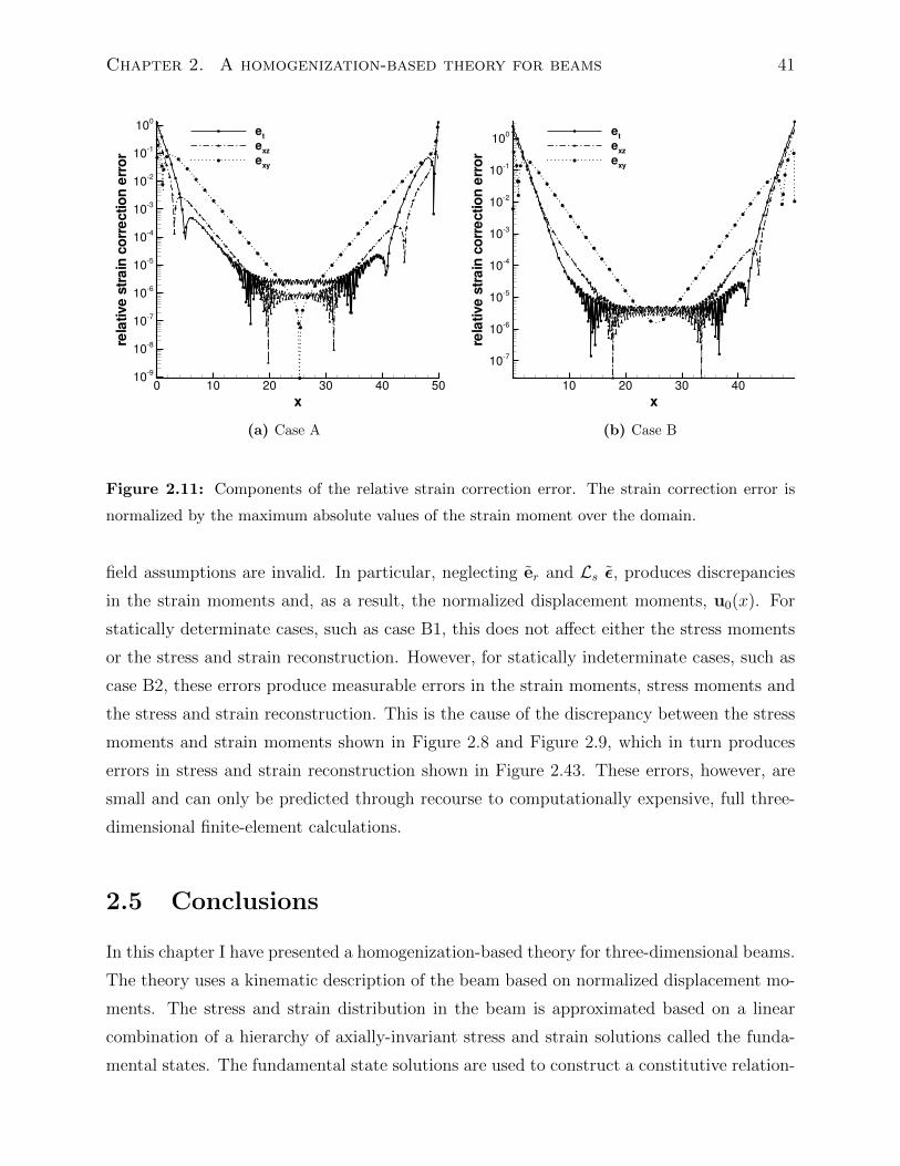
Chapter 2. A homogenization-based theory for beams 41
x
relativestrain
correctionerror
0 10 20 30 40 5010
9
108
107
106
105
104
103
102
101
100
et
exz
exy
(a) Case A
x
relativestrain
correctionerror
10 20 30 40
107
106
105
104
103
102
101
100 e
t
exz
exy
(b) Case B
Figure 2.11: Components of the relative strain correction error. The strain correction error is
normalized by the maximum absolute values of the strain moment over the domain.
field assumptions are invalid. In particular, neglecting er and Ls ε, produces discrepancies
in the strain moments and, as a result, the normalized displacement moments, u0(x). For
statically determinate cases, such as case B1, this does not affect either the stress moments
or the stress and strain reconstruction. However, for statically indeterminate cases, such as
case B2, these errors produce measurable errors in the strain moments, stress moments and
the stress and strain reconstruction. This is the cause of the discrepancy between the stress
moments and strain moments shown in Figure 2.8 and Figure 2.9, which in turn produces
errors in stress and strain reconstruction shown in Figure 2.43. These errors, however, are
small and can only be predicted through recourse to computationally expensive, full three-
dimensional finite-element calculations.
2.5 Conclusions
In this chapter I have presented a homogenization-based theory for three-dimensional beams.
The theory uses a kinematic description of the beam based on normalized displacement mo-
ments. The stress and strain distribution in the beam is approximated based on a linear
combination of a hierarchy of axially-invariant stress and strain solutions called the funda-
mental states. The fundamental state solutions are used to construct a constitutive relation-
Chapter 2. A homogenization-based theory for beams 42
ship between moments of stress and moments strain. The fundamental states are also used
to determine a strain correction matrix that modifies the strain moments predicted by the
normalized displacement moments. For isotropic beams with symmetric cross-sections, the
present beam theory takes the form of classical Timoshenko beam theory with additional
load-dependent stress and strain corrections. For arbitrary, anisotropic sections, the homog-
enized stiffness matrix becomes fully populated and all components of the stress resultants
are coupled.
In addition, I presented a finite-element based method for the calculation of the fun-
damental state solutions, and verified this approach with three-dimensional finite-element
calculations. I demonstrated excellent agreement between the stress and strain distributions
for statically determinate and statically indeterminate problems, achieving extremely high
accuracy away from the ends of the beam. For statically determinate problems, the relative
error of all strain moment components at the center of the beam was less than 10−6, while for
the statically indeterminate beam, the maximum relative error was 2%. The larger error for
the statically indeterminate case was attributed to the moments of the strain residuals and
the strain correction error. Despite this error, the stress and strain reconstruction remains
sufficiently accurate for engineering purposes. In addition, the finite-element based beam
theory calculations required three orders of magnitude less computational time compared to
three-dimensional finite-element computations. These characteristics make the beam the-
ory an attractive approach for accurate through-thickness stress and strain prediction in
composite beams.
Chapter 3
Parallel finite-element analysis of shell
structures
Thin, stiffened shell structures are frequently used in aerospace applications due to their
high stiffness-to-weight and strength-to-weight ratios. Stiffened structures, such as wings
and fuselages, are primarily designed to carry in-plane loads that produce a more uniform
distribution of stress and strain through the thickness than bending loads, resulting in a more
efficient use of material. As with any slender, compressively-loaded structure, structural
instability is often a critical design case and the sizing and placement of stiffeners is often
dictated by buckling considerations.
In this section, I present methods that may be used to efficiently analyze and design
stiffened shell structures appropriate for aerospace applications. In particular, I present
a higher-order shell element formulation for accurate stress and strain prediction, parallel
solution methods for the analysis of large structural models, and efficient and accurate sensi-
tivity analysis techniques for gradient-based optimization. The material in this chapter has
been developed into a unified computational framework called the Toolkit for the Analysis
of Composite Structures (TACS). TACS is written in C++, with a Python-level interface,
and has been built with multidisciplinary analysis and gradient evaluation in mind.
This chapter is organized as follows: in Section 3.1, I present a higher-order shell element
formulation used for the analysis of thin, composite structures. In Section 3.2, I present an
overview of the domain-decomposition-based parallel finite-element approach used in TACS.
In Section 3.3, I present methods to solve the sparse linear systems that arise from the finite-
element discretization of structural problems. Finally, in Section 3.4, I present efficient design
sensitivity methods for use in structural design optimization.
43
Chapter 3. Parallel finite-element analysis of shell structures 44
3.1 Finite-element analysis of shell structures
There are numerous issues that need to be addressed when developing general purpose shell
elements for use on a wide range of shell problems. These issues range from the method
used to formulate the shell element, to problems with the numerical behavior under certain
analysis conditions. I will address the most significant issues below and describe the methods
used to address them.
There are essentially two main approaches that may be used to formulate shell elements.
The first approach is to derive a shell theory, based on a set of kinematic assumptions about
the behavior of the shell, and then apply a finite-element discretization to the resulting shell
theory. There are several examples of this approach in the literature. Perhaps the most
extensive efforts in this area have been undertaken by Simo and Fox [1989], Simo et al.
[1989, 1990a,b] and Simo [1993]. One of the main difficulties with this approach is obtaining
an element that contains the necessary rigid-body rotation and translation modes [Hansen
and Heppler, 1985]. The second approach, first developed by Ahmad et al. [1970], is to
formulate a continuum-based shell element by reducing the full three-dimensional equations
of elasticity to the mid-surface using shell-theory-like assumptions about the distribution of
the displacements through the thickness. This approach is usually referred to as the degener-
ated solid approach. Bathe and Bolourchi [1980], Parisch [1978] and Hughes and Liu [1981]
also extended the degenerated solid approach to nonlinear geometric and nonlinear material
problems. Buechter and Ramm [1992] performed an extensive comparison of shell-element
formulations and showed that both the degenerated solid and shell-formulation approaches
can lead to a mathematically equivalent formulation if the same modeling assumptions are
used.
Another significant challenge associated with the analysis of thin shells, as well as plates
and beams, is a numerical issue known as locking [Babuska and Suri, 1992]. Shear and
membrane locking may occur when using a conforming low-order displacement-based shell
element that employs some form of shear deformation theory to account for the rotation of
the shell-normal during deformation. These types of shell elements do not allow a state of
pure bending and as a result, over-predict the shear strain energy within the shell [Chapelle
and Bathe, 2003]. This additional shear strain energy makes the element stiffer than it should
be, producing small-than-expected displacements. Membrane locking occurs in shells when
coupling exists between in-plane and shear loads. Like shear locking, membrane locking
produces stiffer-than-expected results, even for extremely fine meshes.
Shear and membrane locking are usually addressed by using one of three approaches:
Chapter 3. Parallel finite-element analysis of shell structures 45
higher-order displacement-based elements (typically at least fourth-order), reduced or se-
lective integration of the shear strain energy terms, or the use of mixed formulations. For
instance, Hughes et al. [1977, 1978] used selective, reduced-order integration of the shear
strain energy to alleviate shear locking for low-order elements. However, this approach can
suffer due to the introduction of spurious zero-energy modes, especially for higher-order
elements. Heppler and Hansen [1986] developed a locking-free shell element by using fourth-
order Lagrange interpolation functions for thick shells using Reissner–Mindlin kinematic
assumptions.
Various authors have presented mixed shell element formulations based on mixed energy
principles. In these approaches certain stress or strain components, or the entire stress or
strain field are also included in the finite-element discretization. One of the most successful
mixed-interpolation approaches for shell elements is the technique of using mixed interpola-
tion of tensorial components (MITC) originally developed by Dvorkin and Bathe [1984] and
Bathe and Dvorkin [1985]. In the MITC approach, shear and membrane strains are interpo-
lated based on an appropriate lower-order polynomial. The strain interpolation is forced to
match the displacement-based strain values at the strain interpolation points, called tying
points. While the element formulation is based on an a mixed-energy principle, the element
nodal variables remain the classical displacement and rotation variables. This approach can
also be extended to higher-order element formulations [Bathe and Dvorkin, 1986, Bucalem
and Bathe, 1993]. The MITC formulation was put on a rigorous mathematical foundation
by the analysis of Bathe et al. [2000] and Chapelle and Bathe [2003] using the framework of
Brezzi and Fortin [1991].
I have implemented both a displacement-based shell element and an MITC-based shell el-
ement using a degenerated solid approach. However, this formulation can also be interpreted
as a shell theory formulation based on the work of Buechter and Ramm [1992]. Following
Milford and Schnobrich [1986], the formulation uses an explicit integration of the strain en-
ergy through the thickness, enabling the direct use of the classical first-order deformation
theory (FSDT) constitutive relationships. This explicit integration approach, however, in-
troduces a modeling error on the order of the ratio of the thickness to radius of curvature. As
a result, the shell element is not appropriate for thick shells or shells with high-curvature. In
the present implementation, a small angle approximation is used to represent the rotations
and the drilling degree of freedom is included in the element formulation using the approach
outlined by Hughes and Brezzi [1989].
Chapter 3. Parallel finite-element analysis of shell structures 46
3.1.1 Shell formulation
In this section, I derive the finite-element formulation for a shell using a total Lagrangian
approach based on the degenerated solid technique. The starting point for the derivation is
the principle of virtual work, written here as follows:∫Ω
tr (δεS) dΩ = δW ext, (3.1)
where W ext is the work done by external forces, Ω is the volume of the shell, tr(·) is the
trace operator, S ∈ R3×3 are the components of the second Piola–Kirchhoff stress tensor,
and ε ∈ R3×3 are the components of the Green strain, also referred to as the Green–Lagrange
strain. The constitutive equations, in general, can be written in rate form S′ = C · ε′, where
C ∈ R3×3×3×3 is a fourth-order constitutive tensor that relates the rate of change of strain
ε′ to the rate of change of stress, S′ [Bathe, 1996]. At present, the analysis is limited to
a linear constitutive relationship such that C remains constant, regardless of the stress or
strain fields. As a result, the constitutive relationship is written as follows:
S = C · ε. (3.2)
Note that this is not a matrix-matrix product, but rather an inner product of a fourth and
second order tensors. The Green strain is written as follows:
ε =1
2
(U,x + UT
,x + UT,xU,x
), (3.3)
where U ∈ R3 are the Cartesian displacement components between the initial and deformed
geometry, and x ∈ R3 are the global Cartesian coordinates.
The initial, undeformed geometry of the shell may be described in terms of a reference
surface r(ξ) ∈ R3, the shell thickness h(ξ) ∈ R+ and the unit surface normal vector n(ξ) ∈R3. Here, ξ = [ξ1 ξ2]T is the parametric location on the reference surface. The thickness of
the shell is accounted for with a through-thickness coordinate ζ that is the distance along
the unit normal from the surface, ζ ∈ [−h/2, h/2]. With these definitions, the entire volume
of the shell has the following parametric description:
R(ξ, ζ) = r(ξ) + ζn(ξ), (3.4)
As a result of these definitions, r(ξ) is the mid-surface of the shell. At times it is also
convenient to group the shell parametrization into the vector η = [ξ1 ξ2 ζ]T . The initial and
the deformed geometry of a shell segment are illustrated in Figure 3.1.
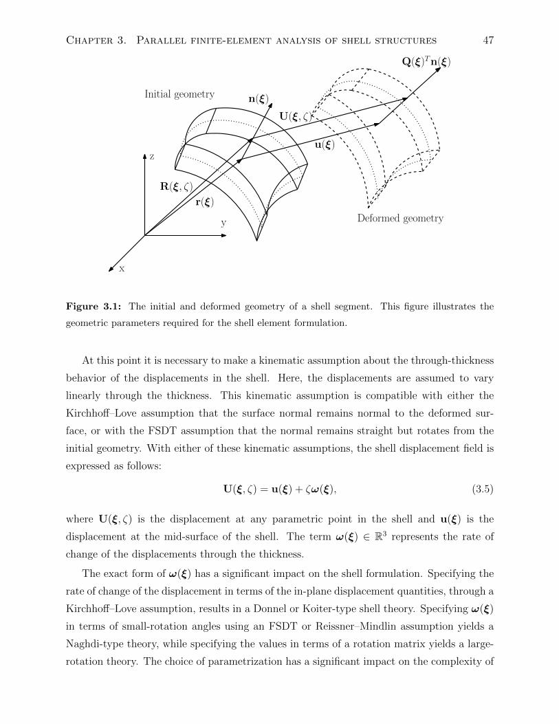
Chapter 3. Parallel finite-element analysis of shell structures 47
x
y
z
r(ξ)
R(ξ, ζ)
n(ξ)
u(ξ)
U(ξ, ζ)
Q(ξ)Tn(ξ)
Initial geometry
Deformed geometry
Figure 3.1: The initial and deformed geometry of a shell segment. This figure illustrates the
geometric parameters required for the shell element formulation.
At this point it is necessary to make a kinematic assumption about the through-thickness
behavior of the displacements in the shell. Here, the displacements are assumed to vary
linearly through the thickness. This kinematic assumption is compatible with either the
Kirchhoff–Love assumption that the surface normal remains normal to the deformed sur-
face, or with the FSDT assumption that the normal remains straight but rotates from the
initial geometry. With either of these kinematic assumptions, the shell displacement field is
expressed as follows:
U(ξ, ζ) = u(ξ) + ζω(ξ), (3.5)
where U(ξ, ζ) is the displacement at any parametric point in the shell and u(ξ) is the
displacement at the mid-surface of the shell. The term ω(ξ) ∈ R3 represents the rate of
change of the displacements through the thickness.
The exact form of ω(ξ) has a significant impact on the shell formulation. Specifying the
rate of change of the displacement in terms of the in-plane displacement quantities, through a
Kirchhoff–Love assumption, results in a Donnel or Koiter-type shell theory. Specifying ω(ξ)
in terms of small-rotation angles using an FSDT or Reissner–Mindlin assumption yields a
Naghdi-type theory, while specifying the values in terms of a rotation matrix yields a large-
rotation theory. The choice of parametrization has a significant impact on the complexity of
Chapter 3. Parallel finite-element analysis of shell structures 48
the strain expressions. In general, ω(ξ) can be expressed as
ω(ξ) =(Q(ξ)T − I
)n(ξ),
where Q(ξ) ∈ R3×3 is a rotation matrix or an approximation of a rotation matrix, I ∈ R3×3
is the identity and n(ξ) is the unit normal of the undeformed geometry. Here, a small-angle
approximation of the rotation matrix is employed, such that Q(ξ)T = I +φ(ξ)×, where (·)×
is the cross-product operator [Hughes, 2004]. The vector φ(ξ) ∈ R3 are small rotations in
the global Cartesian reference frame:
φ(ξ) =[φx φy φz
]T. (3.6)
As a result of this choice of parametrization, the rate of change of the displacements through
the thickness of the shell is
ω(ξ) = φ(ξ)×n(ξ). (3.7)
Throughout the remainder of this section, the variable ω(ξ) is retained in the formulation.
The next step in the derivation is to use the assumed displacement field (3.5) to arrive
at an expression for the strain in the shell. The approach taken here is to express the
displacements in the global Cartesian reference frame while working with the strains in a
local Cartesian reference frame attached to the shell surface. This technique avoids the use of
non-Cartesian tensors that must be employed when the shell displacements are expressed in a
local non-orthogonal reference frame constructed on the shell surface [Buechter and Ramm,
1992]. The transformation between the global and the shell-attached reference frames is
denoted T(ξ) ∈ R3×3, such that the Green strain (3.3) transforms as follows:
εs(η) = T(ξ)ε(η)T(ξ)T , (3.8)
where εs(η) is the Green strain in the shell-attached coordinate frame. The strain in the
locally-attached reference frame takes the form
εs(η) = ε(0)s (ξ) + ζε(1)
s (ξ) + ζ2ε(2)s (ξ), (3.9)
where quadratic coefficient ε(2)s is neglected in all further formula in order to retain consis-
tency with the FSDT assumptions.
Using the relationship for the through-thickness strain distribution (3.9), the strain energy
Chapter 3. Parallel finite-element analysis of shell structures 49
expression in the principle of virtual work (3.1) is written∫A
∫ h/2
−h/2tr((δε(0)
s + ζ δε(1)s
) [C ·(ε(0)s + ζε(1)
s
)])|R,η| dζ dA ≈∫
A
tr(δε(0)
s A · ε(0)s + δε(0)
s B · ε(1)s + δε(1)
s B · ε(0)s + δε(1)
s D · ε(1)s
)|R,η|ζ=0 dA = δW ext,
(3.10)
where A is the area of the shell. Note that the determinant of the Jacobian |R,η| varies
through the thickness of the shell. Instead of computing this integral exactly, the determi-
nant value is fixed to the value at the mid-surface such that |R,η| ≈ |R,η|ζ=0. This is a
reasonable assumption for thin shells, with moderate curvature and simplifies the integra-
tion considerably [Milford and Schnobrich, 1986]. The fourth order tensors A, B and D are
defined as follows:
A =
∫ h/2
−h/2C dζ, B =
∫ h/2
−h/2ζC dζ, D =
∫ h/2
−h/2ζ2C dζ. (3.11)
While all components of the constitutive tensor could be integrated through the thickness
of the shell, in practice conditions consistent with the FSDT assumptions are made when
calculating these integrals. In particular, a plane-stress assumption is imposed, such that
the through-thickness stress is zero, and only those constitutive terms that are associated
with the classical FSDT approach are retained: the in-plane normal and shear terms in A,
B and D, and the out-of-plane shear terms in A. In addition, a shear correction factor is
applied to the out-of-plane shear terms in A.
The main task now is to obtain the Green strain in the global reference frame (3.3), and
transform it to the local reference frame using Equation (3.8). In order to evaluate the strain,
the derivative of the displacements in the global reference frame U,x must be expressed in
terms of the shell parametrization variables η. This derivative is expressed as follows:
U,x = U,ηη,x = U,ηR,η(η)−1. (3.12)
This expression for U,x, is a complicated, nonlinear function of the through-thickness coor-
dinate ζ, due to the inverse Jacobian term R,η(η)−1. Belytschko et al. [1989] and Buechter
and Ramm [1992] found that a linearization of Equation (3.12) is sufficient to retain an
accuracy of order h/R in the strain expressions, where h is the shell thickness and R is the
smallest radius of curvature. Linearizing Equation (3.12) about the mid-surface of the shell
gives
U,x ≈ U(0),x + ζU(1)
,x , (3.13)
Chapter 3. Parallel finite-element analysis of shell structures 50
where U(0),x and U
(1),x are the first and second terms in a Taylor series expansion. These terms
are defined as follows:
U(0),x = U,ηη,x
∣∣ζ=0
= [u,ξ1 u,ξ2 ω]η(0),x ,
U(1),x =
U,ηζη,x + U,ηη,xζ
∣∣ζ=0
= ω,ηη(0),x + [u,ξ1 u,ξ2 ω]η
(0),xζ ,
(3.14)
with η(0),x = R,η(η)−1|ζ=0 and η
(0),xζ = −η(0)
,x n,ηη(0),x . Note that U
(0),x and U
(1),x are independent
of the through-thickness coordinate ζ. With these definitions, the terms in the expansion of
the strain through the thickness (3.9) can be written as follows:
ε(0)s =
1
2T(U(0),x + U(0)
,x
T+ U(0)
,x
TU(0),x
)TT ,
ε(1)s =
1
2T(U(1),x + U(1)
,x
T+ U(1)
,x
TU(0),x + U(0)
,x
TU(1),x
)TT ,
ε(2)s =
1
2TU(1)
,x
TU(1),x TT .
(3.15)
This completes the derivation of the strain and energy expressions required for a displacement-
based shell element. The principle of virtual work (3.10), in conjunction with the strain
expressions (3.14) and (3.15), and the integrated constitutive expressions (3.11) are used to
evaluate the element residuals and, with standard techniques, the geometric and tangent
stiffness matrices [Bathe, 1996, Zienkiewicz et al., 2005]. The assumptions made during the
derivation of the strain expressions are as follows:
1. The displacements vary linearly through the thickness of the shell (3.5)
2. The rate of change of displacements in the through-thickness direction obeys the
Reissner–Mindlin kinematic assumption (3.7)
3. The through-thickness variation of the determinant of the Jacobian |R,η| can be ne-
glected when computing the work integral (3.10)
4. The through-thickness stress is zero resulting in a state of plane-stress in for the inte-
grated constitutive relationship (3.11)
5. The higher-order strain terms ε(2)s from Equation (3.15) can be neglected in the work
integral (3.10)
6. The gradient of the displacement through the thickness can be linearized from Equa-
tion (3.13) with an order h/R error
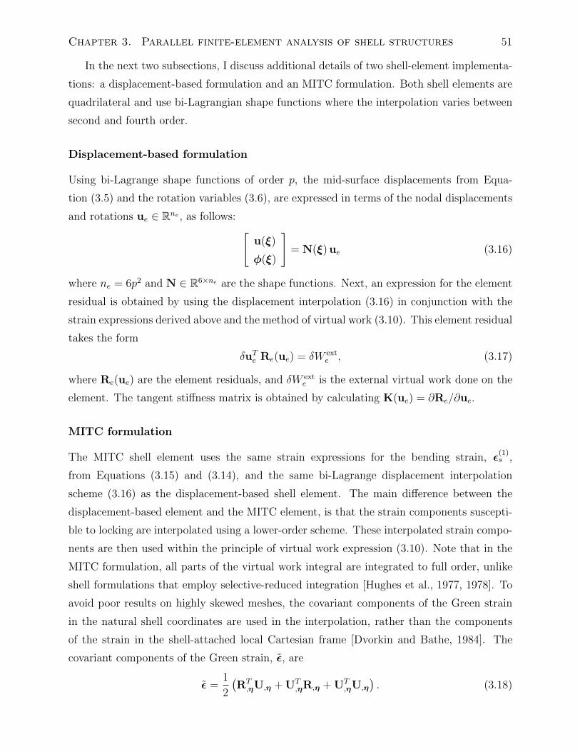
Chapter 3. Parallel finite-element analysis of shell structures 51
In the next two subsections, I discuss additional details of two shell-element implementa-
tions: a displacement-based formulation and an MITC formulation. Both shell elements are
quadrilateral and use bi-Lagrangian shape functions where the interpolation varies between
second and fourth order.
Displacement-based formulation
Using bi-Lagrange shape functions of order p, the mid-surface displacements from Equa-
tion (3.5) and the rotation variables (3.6), are expressed in terms of the nodal displacements
and rotations ue ∈ Rne , as follows: [u(ξ)
φ(ξ)
]= N(ξ) ue (3.16)
where ne = 6p2 and N ∈ R6×ne are the shape functions. Next, an expression for the element
residual is obtained by using the displacement interpolation (3.16) in conjunction with the
strain expressions derived above and the method of virtual work (3.10). This element residual
takes the form
δuTe Re(ue) = δW exte , (3.17)
where Re(ue) are the element residuals, and δW exte is the external virtual work done on the
element. The tangent stiffness matrix is obtained by calculating K(ue) = ∂Re/∂ue.
MITC formulation
The MITC shell element uses the same strain expressions for the bending strain, ε(1)s ,
from Equations (3.15) and (3.14), and the same bi-Lagrange displacement interpolation
scheme (3.16) as the displacement-based shell element. The main difference between the
displacement-based element and the MITC element, is that the strain components suscepti-
ble to locking are interpolated using a lower-order scheme. These interpolated strain compo-
nents are then used within the principle of virtual work expression (3.10). Note that in the
MITC formulation, all parts of the virtual work integral are integrated to full order, unlike
shell formulations that employ selective-reduced integration [Hughes et al., 1977, 1978]. To
avoid poor results on highly skewed meshes, the covariant components of the Green strain
in the natural shell coordinates are used in the interpolation, rather than the components
of the strain in the shell-attached local Cartesian frame [Dvorkin and Bathe, 1984]. The
covariant components of the Green strain, ε, are
ε =1
2
(RT,ηU,η + UT
,ηR,η + UT,ηU,η
). (3.18)
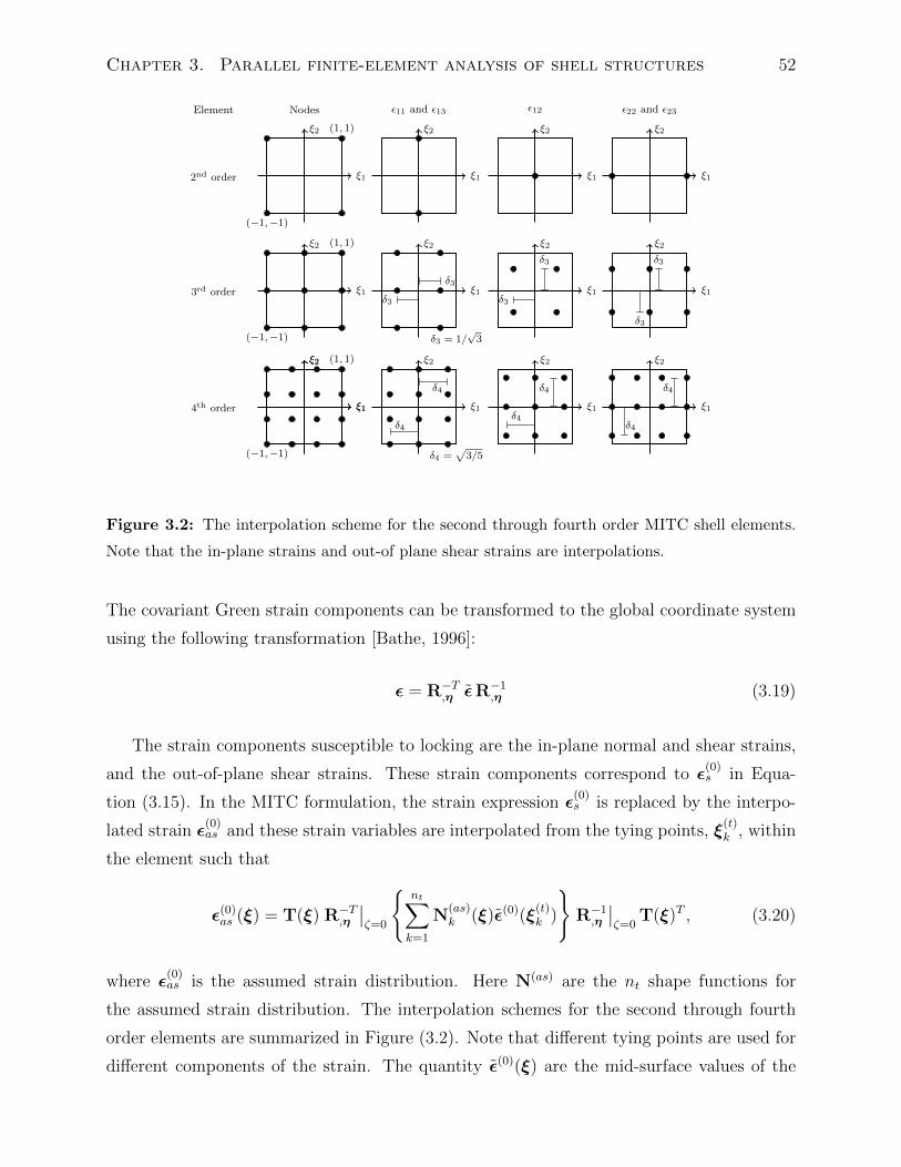
Chapter 3. Parallel finite-element analysis of shell structures 52
Element Nodes ε11 and ε13 ε12 ε22 and ε23
2nd order
ξ2
ξ1
(−1,−1)
(1, 1) ξ2
ξ1
ξ2
ξ1
ξ2
ξ1
3rd order
ξ2
ξ1
(−1,−1)
(1, 1) ξ2
ξ1
δ3 = 1/√3
δ3
δ3
ξ2
ξ1δ3
δ3
ξ2
ξ1
δ3
δ3
4th order
ξ2
ξ1
(−1,−1)
(1, 1)ξ2
ξ1
δ4
δ4
δ4 =√
3/5
ξ2
ξ1δ4
δ4
ξ2
ξ1
δ4
δ4
ξ2
ξ1
Figure 3.2: The interpolation scheme for the second through fourth order MITC shell elements.
Note that the in-plane strains and out-of plane shear strains are interpolations.
The covariant Green strain components can be transformed to the global coordinate system
using the following transformation [Bathe, 1996]:
ε = R−T,η εR−1,η (3.19)
The strain components susceptible to locking are the in-plane normal and shear strains,
and the out-of-plane shear strains. These strain components correspond to ε(0)s in Equa-
tion (3.15). In the MITC formulation, the strain expression ε(0)s is replaced by the interpo-
lated strain ε(0)as and these strain variables are interpolated from the tying points, ξ
(t)k , within
the element such that
ε(0)as (ξ) = T(ξ) R−T,η
∣∣ζ=0
nt∑k=1
N(as)k (ξ)ε(0)(ξ
(t)k )
R−1,η
∣∣ζ=0
T(ξ)T , (3.20)
where ε(0)as is the assumed strain distribution. Here N(as) are the nt shape functions for
the assumed strain distribution. The interpolation schemes for the second through fourth
order elements are summarized in Figure (3.2). Note that different tying points are used for
different components of the strain. The quantity ε(0)(ξ) are the mid-surface values of the
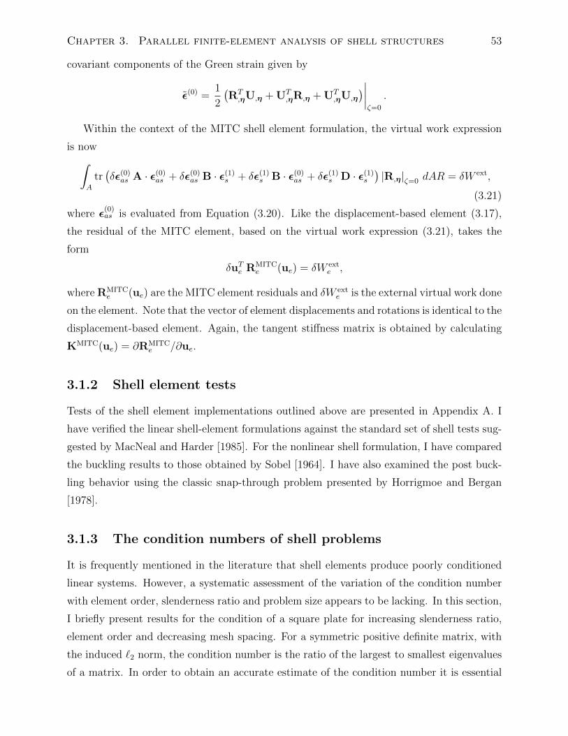
Chapter 3. Parallel finite-element analysis of shell structures 53
covariant components of the Green strain given by
ε(0) =1
2
(RT,ηU,η + UT
,ηR,η + UT,ηU,η
)∣∣∣∣ζ=0
.
Within the context of the MITC shell element formulation, the virtual work expression
is now∫A
tr(δε(0)
as A · ε(0)as + δε(0)
as B · ε(1)s + δε(1)
s B · ε(0)as + δε(1)
s D · ε(1)s
)|R,η|ζ=0 dAR = δW ext,
(3.21)
where ε(0)as is evaluated from Equation (3.20). Like the displacement-based element (3.17),
the residual of the MITC element, based on the virtual work expression (3.21), takes the
form
δuTe RMITCe (ue) = δW ext
e ,
where RMITCe (ue) are the MITC element residuals and δW ext
e is the external virtual work done
on the element. Note that the vector of element displacements and rotations is identical to the
displacement-based element. Again, the tangent stiffness matrix is obtained by calculating
KMITC(ue) = ∂RMITCe /∂ue.
3.1.2 Shell element tests
Tests of the shell element implementations outlined above are presented in Appendix A. I
have verified the linear shell-element formulations against the standard set of shell tests sug-
gested by MacNeal and Harder [1985]. For the nonlinear shell formulation, I have compared
the buckling results to those obtained by Sobel [1964]. I have also examined the post buck-
ling behavior using the classic snap-through problem presented by Horrigmoe and Bergan
[1978].
3.1.3 The condition numbers of shell problems
It is frequently mentioned in the literature that shell elements produce poorly conditioned
linear systems. However, a systematic assessment of the variation of the condition number
with element order, slenderness ratio and problem size appears to be lacking. In this section,
I briefly present results for the condition of a square plate for increasing slenderness ratio,
element order and decreasing mesh spacing. For a symmetric positive definite matrix, with
the induced `2 norm, the condition number is the ratio of the largest to smallest eigenvalues
of a matrix. In order to obtain an accurate estimate of the condition number it is essential
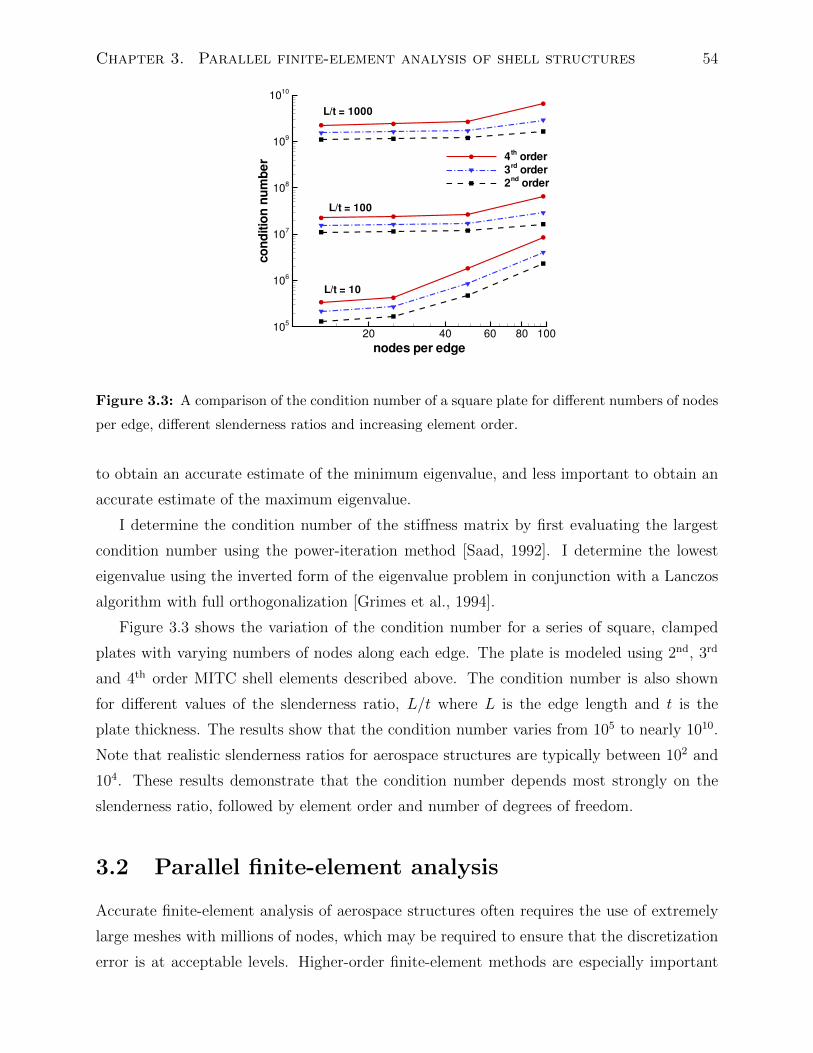
Chapter 3. Parallel finite-element analysis of shell structures 54
nodes per edge
conditionnumber
20 40 60 80 10010
5
106
107
108
109
1010
4thorder
3rdorder
2ndorder
L/t = 10
L/t = 100
L/t = 1000
Figure 3.3: A comparison of the condition number of a square plate for different numbers of nodes
per edge, different slenderness ratios and increasing element order.
to obtain an accurate estimate of the minimum eigenvalue, and less important to obtain an
accurate estimate of the maximum eigenvalue.
I determine the condition number of the stiffness matrix by first evaluating the largest
condition number using the power-iteration method [Saad, 1992]. I determine the lowest
eigenvalue using the inverted form of the eigenvalue problem in conjunction with a Lanczos
algorithm with full orthogonalization [Grimes et al., 1994].
Figure 3.3 shows the variation of the condition number for a series of square, clamped
plates with varying numbers of nodes along each edge. The plate is modeled using 2nd, 3rd
and 4th order MITC shell elements described above. The condition number is also shown
for different values of the slenderness ratio, L/t where L is the edge length and t is the
plate thickness. The results show that the condition number varies from 105 to nearly 1010.
Note that realistic slenderness ratios for aerospace structures are typically between 102 and
104. These results demonstrate that the condition number depends most strongly on the
slenderness ratio, followed by element order and number of degrees of freedom.
3.2 Parallel finite-element analysis
Accurate finite-element analysis of aerospace structures often requires the use of extremely
large meshes with millions of nodes, which may be required to ensure that the discretization
error is at acceptable levels. Higher-order finite-element methods are especially important
Chapter 3. Parallel finite-element analysis of shell structures 55
when accurate stress and strain prediction is required, due to the fact that for displacement-
based finite-element formulations, the stress and strain fields converge at a rate that is
one order lower than the convergence rate of the displacement field [Strang and Fix, 1973].
Large finite-element models require specialized solvers that can accurately and robustly
find a solution, even to very poorly conditioned problems. Finite-element problems with
millions of degrees of freedom can only be solved within a time frame that is practical for
optimization purposes using parallel solution methods. As a result, I only consider parallel
solution techniques.
To perform finite-element analysis and design optimization in a parallel computing envi-
ronment, it is necessary to perform the following three operations in parallel:
1. Assemble the global residual vector and global finite-element matrices,
2. Solve linear systems arising from the finite-element discretization,
3. Evaluate functions of interest, and their gradients.
In order to parallelize these three types of operations, I use an element-based partition of
the finite-element mesh. In this approach, each element is assigned to a unique processor.
The variables and nodes required by the elements on a processor are stored locally and as
a result, nodes and variables on domain boundaries are duplicated on multiple processors.
This duplication allows the element residual and element matrix computations to take place
concurrently without communication. Furthermore, functions of interest that require cal-
culations for each element in the mesh can be calculated in parallel. The disadvantage of
the element-based partition approach is that residual components must be communicated
to other processors during the final global residual assembly. However, typically the ratio of
non-local to local residual components is small, and the parallel performance is excellent.
I have carefully implemented the three types of operations outlined above in parallel. Of
these three operations, the parallel solution of linear systems is by far the most complex and
is the exclusive topic of Section 3.3. The evaluation of the gradients of functions of interest
in parallel is discussed in Section 3.4.
3.3 Parallel solution methods for sparse linear systems
Sparse linear systems of the form,
Ax = b, (3.22)
Chapter 3. Parallel finite-element analysis of shell structures 56
arise in the analysis of linear and nonlinear static finite-element problems 1. Furthermore, ac-
celeration techniques used in eigenvalue solvers for modal and buckling analysis, often require
the solution of sparse linear systems of the form (3.22) [Saad, 1992]. Therefore, depending on
the context, the matrix A ∈ Rn×n may be the stiffness matrix, tangent stiffness matrix, an
approximate Jacobian or some linear combination of matrices as required by an eigenvalue
solver or nonlinear solution algorithm. The vectors x, b ∈ Rn are the solution vector and
right hand side, respectively. The sparse matrices that are derived from the finite-element
analysis of structural problems are typically symmetric due to underlying energy principles.
However, follower forces, such as fluid pressure loads, are non-conservative and generate non-
symmetric terms in the structural Jacobian [Elishakoff, 2005]. Since aerostructural problems
are a primary focus of this thesis, I have exclusively implemented techniques that do not
assume that the matrix A is symmetric.
Solution methods for sparse linear systems may be divided into two categories: iterative
methods and direct methods. Direct methods use different variants of Gaussian elimination
to factor the matrix A into a lower-triangular matrix L and an upper-triangular matrix
U such that A = LU. Different variants of Gaussian elimination that employ pivoting
strategies for numerical stability use permutation matrices that modify this simple formula.
Iterative methods find an approximate solution to the linear system (3.22) using an iterative
algorithm [Saad, 2003]. Iterative methods have the advantage that they may satisfy a given
solution criterion in less computational time and typically require significantly less memory
than direct methods. However, direct methods have the advantage that they are robust and
can find a solution to Equation (3.22), even for very poorly conditioned linear systems.
In this work, I have investigated both iterative Krylov subspace methods and direct so-
lution methods for solving the linear system of equations (3.22). In order to unify these
different solution techniques, I always use an iterative Krylov subspace method, with either
a conventional preconditioning method, or a direct solver as a preconditioner. Direct solution
methods are not preconditioners in the classical sense since they are expensive to compute
and expensive to apply to a right-hand-side when compared to other preconditioning tech-
niques. However, Krylov subspace methods are frequently used for iterative refinement of
solutions obtained from direct solvers [Li and Demmel, 2003]. In these applications, the
direct solver is a preconditioner. This unified approach has two main advantages: First, it is
transparent to any multidisciplinary solver that may itself use an iterative technique. Sec-
ond, frequently it is necessary to solve a series of linear systems that are slightly perturbed
1Note that in this section I employ the standard notation for linear systems used in the literature whereA is the matrix, x are unknowns, and b is the right-hand-side.
Chapter 3. Parallel finite-element analysis of shell structures 57
from equation (3.22). In this case, it is often more efficient to solve the perturbed linear
system using a Krylov subspace method without performing an additional factorization.
The remainder of this section is structured as follows: first, I briefly outline relevant
work on direct solution algorithms. Next, I describe the implementation of two parallel
preconditioning methods: the additive Schwarz and approximate Schur preconditioners, and
the implementation of a direct solver: the direct Schur method. In the last section, I examine
the parallel performance of these methods on two large finite-element problems.
Direct solvers
Relatively recently, there has been a renewed interest in direct solution methods for sparse
linear systems, with a focus on parallel implementations. Amestoy et al. [2000], developed
MUMPS (MUltifrontal Massively Parallel Solver), that uses a multi-frontal matrix factor-
ization approach with a right-looking pivot strategy to ensure numerical stability. Once the
frontal matrices reach a certain size, they are factored across groups of processors using a
row-oriented storage format. Finally, the root frontal matrix is factored in parallel using
a 2D block-cyclic dense factorization algorithm. The direct solver SPOOLES (SParse Ob-
ject Oriented Linear Equations Solver) developed by Ashcraft and Grimes [1999] also uses a
multi-frontal factorization approach. SPOOLES achieves parallelism by performing a recur-
sive nested dissection algorithm on the original matrix graph, determining the parts of the
matrix that can be factored independently.
Demmel et al. [1999], Li and Demmel [2003] developed SuperLU and SuperLU DIST,
sequential and parallel distributed direct solvers, respectively, for both symmetric and non-
symmetric linear systems. SuperLU DIST uses a block-cyclic format where the size of the
blocks are determined based on a super-node analysis of the initial matrix. SuperLU DIST
does not perform pivoting for stability, but instead uses various pre-processing operations
to enhance the numerical properties of the matrix. Parallelism during the factorization is
achieved by distributing the trailing-matrix update and performing the update in a process
queue.
3.3.1 Additive Schwarz and approximate Schur preconditioners
The additive Schwarz and approximate Schur preconditioners both employ a row-oriented
matrix storage scheme. In this scheme, each processor is assigned a contiguous segment of
the rows from the linear system (3.22), while the unknowns are assigned to one of three
groups:
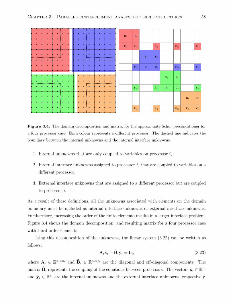
Chapter 3. Parallel finite-element analysis of shell structures 58
B1 E1
F1 C1 F12 F13 F14
B2 E2
F21 F2 C2 F23 F24
B3 E3
F31 F32 F3 C3 F34
B4 E4
F41 F42 F43 F4 C4
Figure 3.4: The domain decomposition and matrix for the approximate Schur preconditioner for
a four processor case. Each colour represents a different processor. The dashed line indicates the
boundary between the internal unknowns and the internal interface unknowns.
1. Internal unknowns that are only coupled to variables on processor i,
2. Internal interface unknowns assigned to processor i, that are coupled to variables on a
different processor,
3. External interface unknowns that are assigned to a different processor but are coupled
to processor i.
As a result of these definitions, all the unknowns associated with elements on the domain
boundary must be included as internal interface unknowns or external interface unknowns.
Furthermore, increasing the order of the finite-elements results in a larger interface problem.
Figure 3.4 shows the domain decomposition, and resulting matrix for a four processor case
with third-order elements.
Using this decomposition of the unknowns, the linear system (3.22) can be written as
follows:
Aixi + Biyi = bi, (3.23)
where Ai ∈ Rni×ni and Bi ∈ Rni×pi are the diagonal and off-diagonal components. The
matrix Bi represents the coupling of the equations between processors. The vectors xi ∈ Rni
and yi ∈ Rpi are the internal unknowns and the external interface unknowns, respectively.
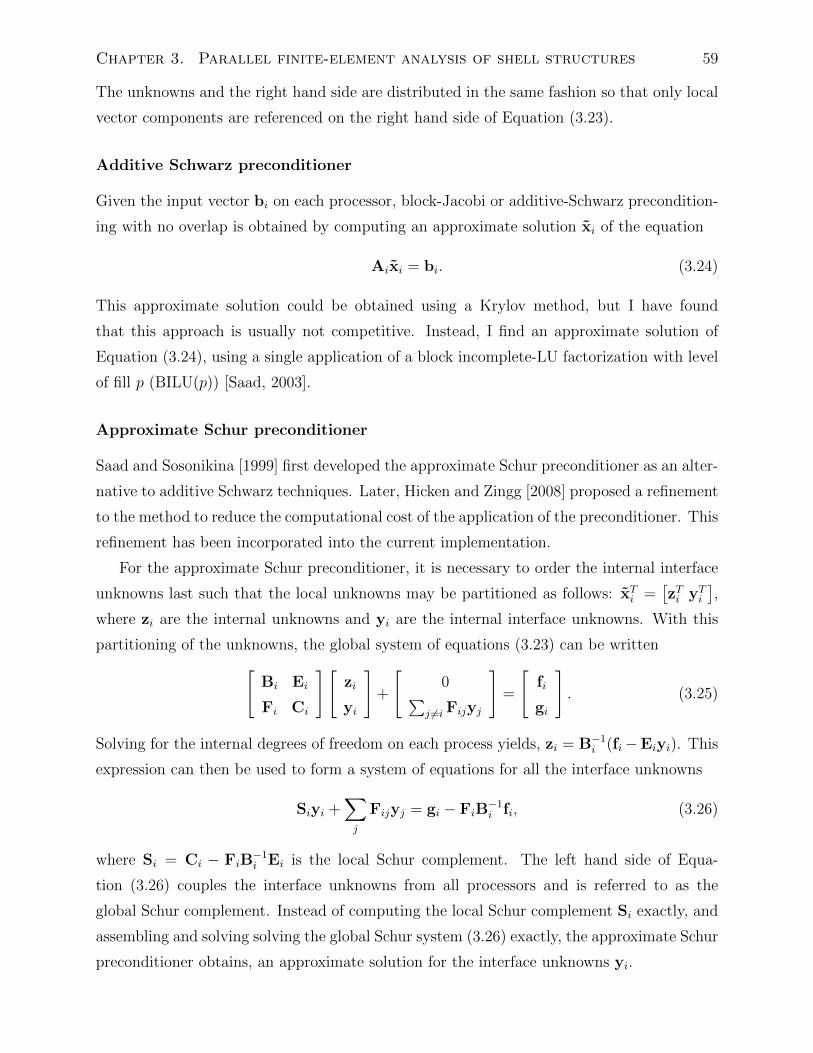
Chapter 3. Parallel finite-element analysis of shell structures 59
The unknowns and the right hand side are distributed in the same fashion so that only local
vector components are referenced on the right hand side of Equation (3.23).
Additive Schwarz preconditioner
Given the input vector bi on each processor, block-Jacobi or additive-Schwarz precondition-
ing with no overlap is obtained by computing an approximate solution xi of the equation
Aixi = bi. (3.24)
This approximate solution could be obtained using a Krylov method, but I have found
that this approach is usually not competitive. Instead, I find an approximate solution of
Equation (3.24), using a single application of a block incomplete-LU factorization with level
of fill p (BILU(p)) [Saad, 2003].
Approximate Schur preconditioner
Saad and Sosonikina [1999] first developed the approximate Schur preconditioner as an alter-
native to additive Schwarz techniques. Later, Hicken and Zingg [2008] proposed a refinement
to the method to reduce the computational cost of the application of the preconditioner. This
refinement has been incorporated into the current implementation.
For the approximate Schur preconditioner, it is necessary to order the internal interface
unknowns last such that the local unknowns may be partitioned as follows: xTi =[zTi yTi
],
where zi are the internal unknowns and yi are the internal interface unknowns. With this
partitioning of the unknowns, the global system of equations (3.23) can be written[Bi Ei
Fi Ci
][zi
yi
]+
[0∑
j 6=i Fijyj
]=
[fi
gi
]. (3.25)
Solving for the internal degrees of freedom on each process yields, zi = B−1i (fi−Eiyi). This
expression can then be used to form a system of equations for all the interface unknowns
Siyi +∑j
Fijyj = gi − FiB−1i fi, (3.26)
where Si = Ci − FiB−1i Ei is the local Schur complement. The left hand side of Equa-
tion (3.26) couples the interface unknowns from all processors and is referred to as the
global Schur complement. Instead of computing the local Schur complement Si exactly, and
assembling and solving solving the global Schur system (3.26) exactly, the approximate Schur
preconditioner obtains, an approximate solution for the interface unknowns yi.
Chapter 3. Parallel finite-element analysis of shell structures 60
An approximate global Schur complement system can be obtained by considering an
incomplete LU factorization of the local matrix Ai from Equation (3.25):[Bi Ei
Fi Ci
]=
[LBi 0
FiUB−1i LSi
][UBi LB
−1i Ei
0 USi
]+ R, (3.27)
where R is a matrix of residual entries. Here, I perform this approximate factorization using
BILU(p) [Saad, 2003]. The BILU(p) factorization produces an approximate factorization
of the local Schur complement Si ≈ LSiUSi as a by-product, when the internal interface
variables are ordered last [Saad and Sosonikina, 1999]. The approximate factorization of the
local Schur complement can be used to construct a system of equations closely approximating
Equation (3.26) as follows:
yi + US−1i LS
−1i
∑j
Fijyj = g′i = US−1i LS
−1i
(gi − FiB
−1i fi). (3.28)
In the approximate Schur preconditioner, this system is solved to a loose tolerance using
GMRES [Saad and Schultz, 1986]. Typically, I use GMRES(10) with no restart with a
relative solution tolerance of 10−3. After the interface unknowns yi have been obtained, the
internal unknowns zi are obtained by calculating zi = U−1Bi
L−1Bi
(fi − Eiyi).
The steps in the application of the approximate Schur preconditioner are:
1. Determine the right hand side of Equation (3.28), g′i = US−1i LS
−1i (gi − FiB
−1i fi)
2. Approximately solve Equation (3.28) for the interface unknowns yi using GMRES.
3. Determine the internal unknowns zi = UB−1i LB
−1i (fi − Eiyi)
Note that the cost of factoring the approximate Schur and additive Schwarz precondi-
tioners is the same if the same ordering of Ai is used in both cases.
3.3.2 The direct Schur method
In the following section, I describe the implementation of the direct Schur method. This
method is a domain-decomposition based approach that shares some similarities with multi-
frontal direct factorization methods such as MUMPS [Amestoy et al., 2000] and SPOOLES
[Ashcraft and Grimes, 1999]. In contrast to these methods, however, the global elimination
tree is constrained by the element-based decomposition. While this restricts the parallelism
within the algorithm, it enables better parallel performance of other operations required for
finite-element analysis. In addition, the direct Schur approach also uses a sparse block-cyclic
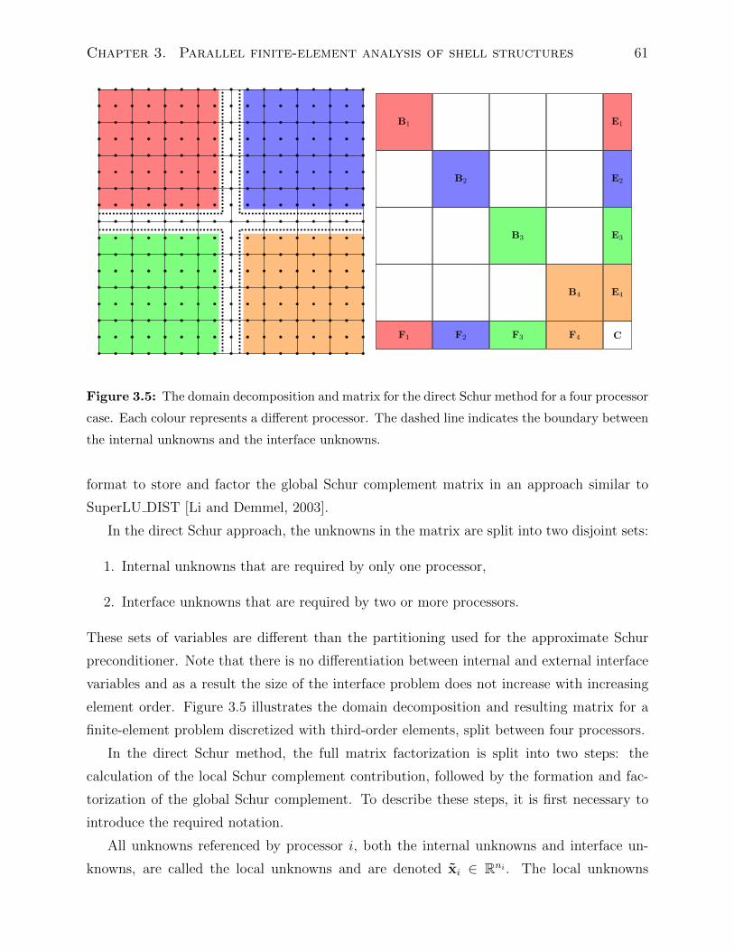
Chapter 3. Parallel finite-element analysis of shell structures 61
B1 E1
B2 E2
B3 E3
B4 E4
F1 F2 F3 F4 C
Figure 3.5: The domain decomposition and matrix for the direct Schur method for a four processor
case. Each colour represents a different processor. The dashed line indicates the boundary between
the internal unknowns and the interface unknowns.
format to store and factor the global Schur complement matrix in an approach similar to
SuperLU DIST [Li and Demmel, 2003].
In the direct Schur approach, the unknowns in the matrix are split into two disjoint sets:
1. Internal unknowns that are required by only one processor,
2. Interface unknowns that are required by two or more processors.
These sets of variables are different than the partitioning used for the approximate Schur
preconditioner. Note that there is no differentiation between internal and external interface
variables and as a result the size of the interface problem does not increase with increasing
element order. Figure 3.5 illustrates the domain decomposition and resulting matrix for a
finite-element problem discretized with third-order elements, split between four processors.
In the direct Schur method, the full matrix factorization is split into two steps: the
calculation of the local Schur complement contribution, followed by the formation and fac-
torization of the global Schur complement. To describe these steps, it is first necessary to
introduce the required notation.
All unknowns referenced by processor i, both the internal unknowns and interface un-
knowns, are called the local unknowns and are denoted xi ∈ Rni . The local unknowns
Chapter 3. Parallel finite-element analysis of shell structures 62
for processor i are be obtained from the global state vector x using a restriction operator
Ri ∈ Rni×n, such that xi = Rix. The local contributions to the matrix A are assembled
from the finite-elements assigned to each processor. These contributions form a local matrix,
Ai ∈ Rni×ni that is related to the global system of equations (3.22) in the following manner:
Ai = RiARTi . (3.29)
In practice, the matrix Ai is assembled on each processor from the local finite-elements
without any communication.
The internal unknowns, denoted zi ∈ Rmi , and the interface unknowns, denoted yi ∈ Rpi ,
are obtained from the local unknowns, xi, using the restriction operators Pi ∈ Rmi×ni and
Qi ∈ Rpi×ni , such that zi = Pixi and yi = Qixi. Instead of forming Ai in an arbitrary
order, the local matrix Ai is split into four block matrices in the following manner:[Bi Ei
Fi Ci
]=
[Pi
Qi
]Ai
[PTi QT
i
], (3.30)
where the dimensions of the matrices Bi, Ei, Fi and Ci can be inferred from the sizes of the
vectors of internal and interface unknowns.
The permutation matrices Pi and Qi are determined to reduce the fill-in during factor-
ization. I have tested three different ordering algorithms: the approximate minimum degree
(AMD) algorithm of Amestoy et al. [1996], and the nested dissection (ND) algorithm in
METIS of Karypis and Kumar [1998]. I have also implemented my own variant of AMD,
based on the work of Amestoy et al. [1996], that takes into account the off-diagonal fill-
ins not considered by the AMD and ND algorithms. I refer to this alternative scheme as
AMD-OD. The AMD and ND orderings determine the permutation matrices Pi and Qi
independently by working only with the diagonal matrices Bi and Ci, respectively. In the
AMD-OD method, Pi and Qi are computed concurrently and the fill-ins produced in the
off-diagonal matrices Ei and Fi are taken into account. This non-standard modification
results in a lower overall fill-in during the factorization process than independently ordering
the internal and interface unknowns.
Using the LU-factorization of the block matrix Bi = LBiUBi
, the local Schur complement
Si can be formed as follows:
Si = Ci − FiU−1Bi
L−1Bi
Ei. (3.31)
Note that both the LU-factorization of the block matrix Bi, and the computation of the local
Schur complement (3.31) can be computed independently, without communication between
processors.
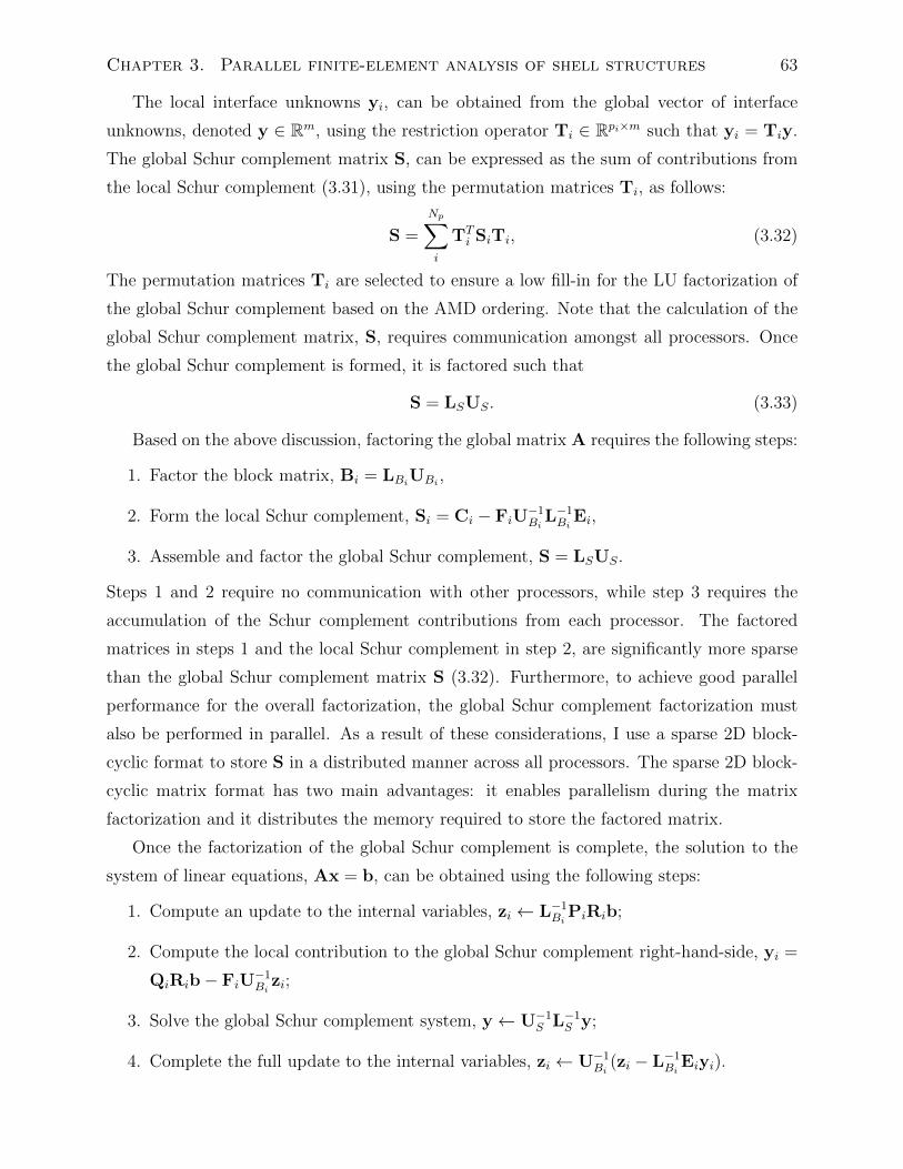
Chapter 3. Parallel finite-element analysis of shell structures 63
The local interface unknowns yi, can be obtained from the global vector of interface
unknowns, denoted y ∈ Rm, using the restriction operator Ti ∈ Rpi×m such that yi = Tiy.
The global Schur complement matrix S, can be expressed as the sum of contributions from
the local Schur complement (3.31), using the permutation matrices Ti, as follows:
S =
Np∑i
TTi SiTi, (3.32)
The permutation matrices Ti are selected to ensure a low fill-in for the LU factorization of
the global Schur complement based on the AMD ordering. Note that the calculation of the
global Schur complement matrix, S, requires communication amongst all processors. Once
the global Schur complement is formed, it is factored such that
S = LSUS. (3.33)
Based on the above discussion, factoring the global matrix A requires the following steps:
1. Factor the block matrix, Bi = LBiUBi
,
2. Form the local Schur complement, Si = Ci − FiU−1Bi
L−1Bi
Ei,
3. Assemble and factor the global Schur complement, S = LSUS.
Steps 1 and 2 require no communication with other processors, while step 3 requires the
accumulation of the Schur complement contributions from each processor. The factored
matrices in steps 1 and the local Schur complement in step 2, are significantly more sparse
than the global Schur complement matrix S (3.32). Furthermore, to achieve good parallel
performance for the overall factorization, the global Schur complement factorization must
also be performed in parallel. As a result of these considerations, I use a sparse 2D block-
cyclic format to store S in a distributed manner across all processors. The sparse 2D block-
cyclic matrix format has two main advantages: it enables parallelism during the matrix
factorization and it distributes the memory required to store the factored matrix.
Once the factorization of the global Schur complement is complete, the solution to the
system of linear equations, Ax = b, can be obtained using the following steps:
1. Compute an update to the internal variables, zi ← L−1Bi
PiRib;
2. Compute the local contribution to the global Schur complement right-hand-side, yi =
QiRib− FiU−1Bi
zi;
3. Solve the global Schur complement system, y← U−1S L−1
S y;
4. Complete the full update to the internal variables, zi ← U−1Bi
(zi − L−1Bi
Eiyi).
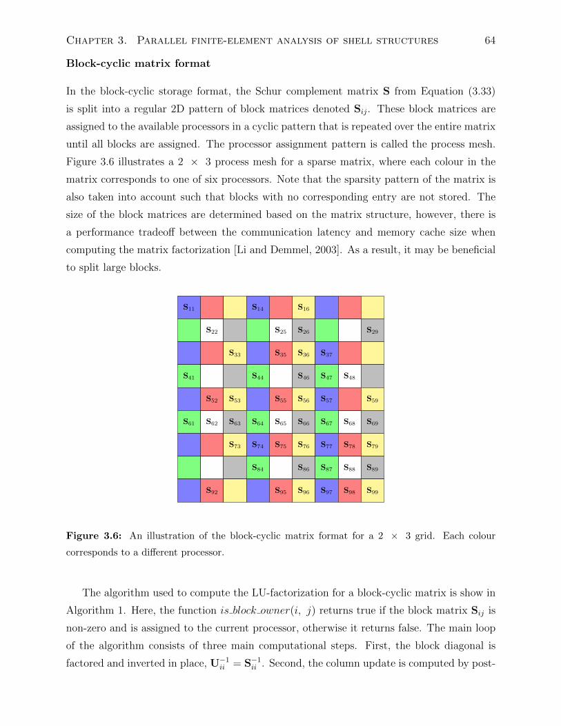
Chapter 3. Parallel finite-element analysis of shell structures 64
Block-cyclic matrix format
In the block-cyclic storage format, the Schur complement matrix S from Equation (3.33)
is split into a regular 2D pattern of block matrices denoted Sij. These block matrices are
assigned to the available processors in a cyclic pattern that is repeated over the entire matrix
until all blocks are assigned. The processor assignment pattern is called the process mesh.
Figure 3.6 illustrates a 2 × 3 process mesh for a sparse matrix, where each colour in the
matrix corresponds to one of six processors. Note that the sparsity pattern of the matrix is
also taken into account such that blocks with no corresponding entry are not stored. The
size of the block matrices are determined based on the matrix structure, however, there is
a performance tradeoff between the communication latency and memory cache size when
computing the matrix factorization [Li and Demmel, 2003]. As a result, it may be beneficial
to split large blocks.
S11 S14 S16
S22 S25 S26 S29
S33 S35 S36 S37
S41 S44 S46 S47 S48
S52 S53 S55 S56 S57 S59
S61 S62 S63 S64 S65 S66 S67 S68 S69
S73 S74 S75 S76 S77 S78 S79
S84 S86 S87 S88 S89
S92 S95 S96 S97 S98 S99
Figure 3.6: An illustration of the block-cyclic matrix format for a 2 × 3 grid. Each colour
corresponds to a different processor.
The algorithm used to compute the LU-factorization for a block-cyclic matrix is show in
Algorithm 1. Here, the function is block owner(i, j) returns true if the block matrix Sij is
non-zero and is assigned to the current processor, otherwise it returns false. The main loop
of the algorithm consists of three main computational steps. First, the block diagonal is
factored and inverted in place, U−1ii = S−1
ii . Second, the column update is computed by post-
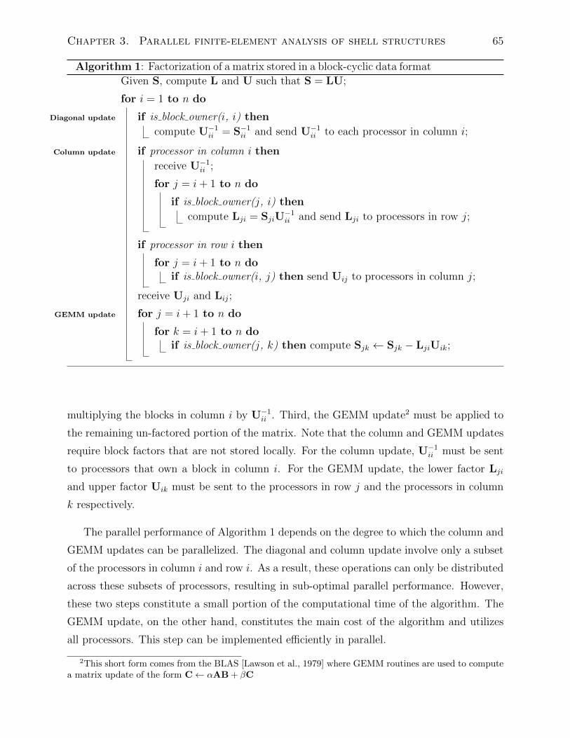
Chapter 3. Parallel finite-element analysis of shell structures 65
Algorithm 1: Factorization of a matrix stored in a block-cyclic data format
Given S, compute L and U such that S = LU;
for i = 1 to n do
Diagonal update if is block owner(i, i) then
compute U−1ii = S−1
ii and send U−1ii to each processor in column i;
Column update if processor in column i then
receive U−1ii ;
for j = i+ 1 to n do
if is block owner(j, i) then
compute Lji = SjiU−1ii and send Lji to processors in row j;
if processor in row i then
for j = i+ 1 to n doif is block owner(i, j) then send Uij to processors in column j;
receive Uji and Lij;
GEMM update for j = i+ 1 to n do
for k = i+ 1 to n doif is block owner(j, k) then compute Sjk ← Sjk − LjiUik;
multiplying the blocks in column i by U−1ii . Third, the GEMM update2 must be applied to
the remaining un-factored portion of the matrix. Note that the column and GEMM updates
require block factors that are not stored locally. For the column update, U−1ii must be sent
to processors that own a block in column i. For the GEMM update, the lower factor Lji
and upper factor Uik must be sent to the processors in row j and the processors in column
k respectively.
The parallel performance of Algorithm 1 depends on the degree to which the column and
GEMM updates can be parallelized. The diagonal and column update involve only a subset
of the processors in column i and row i. As a result, these operations can only be distributed
across these subsets of processors, resulting in sub-optimal parallel performance. However,
these two steps constitute a small portion of the computational time of the algorithm. The
GEMM update, on the other hand, constitutes the main cost of the algorithm and utilizes
all processors. This step can be implemented efficiently in parallel.
2This short form comes from the BLAS [Lawson et al., 1979] where GEMM routines are used to computea matrix update of the form C← αAB + βC
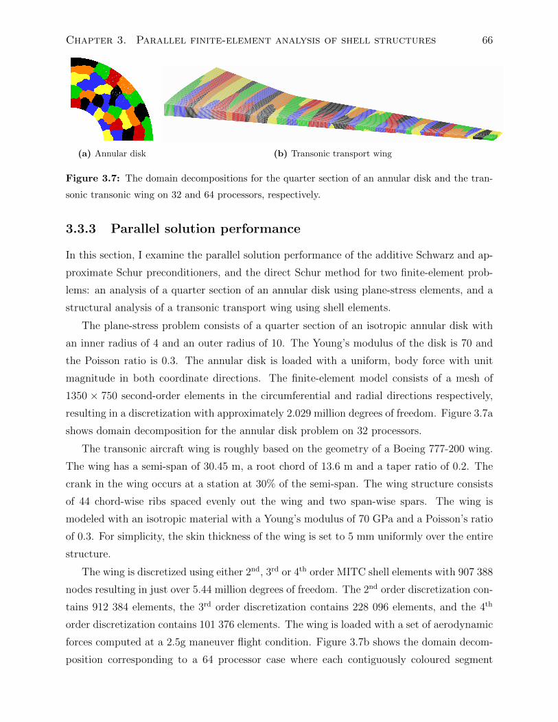
Chapter 3. Parallel finite-element analysis of shell structures 66
(a) Annular disk (b) Transonic transport wing
Figure 3.7: The domain decompositions for the quarter section of an annular disk and the tran-
sonic transonic wing on 32 and 64 processors, respectively.
3.3.3 Parallel solution performance
In this section, I examine the parallel solution performance of the additive Schwarz and ap-
proximate Schur preconditioners, and the direct Schur method for two finite-element prob-
lems: an analysis of a quarter section of an annular disk using plane-stress elements, and a
structural analysis of a transonic transport wing using shell elements.
The plane-stress problem consists of a quarter section of an isotropic annular disk with
an inner radius of 4 and an outer radius of 10. The Young’s modulus of the disk is 70 and
the Poisson ratio is 0.3. The annular disk is loaded with a uniform, body force with unit
magnitude in both coordinate directions. The finite-element model consists of a mesh of
1350 × 750 second-order elements in the circumferential and radial directions respectively,
resulting in a discretization with approximately 2.029 million degrees of freedom. Figure 3.7a
shows domain decomposition for the annular disk problem on 32 processors.
The transonic aircraft wing is roughly based on the geometry of a Boeing 777-200 wing.
The wing has a semi-span of 30.45 m, a root chord of 13.6 m and a taper ratio of 0.2. The
crank in the wing occurs at a station at 30% of the semi-span. The wing structure consists
of 44 chord-wise ribs spaced evenly out the wing and two span-wise spars. The wing is
modeled with an isotropic material with a Young’s modulus of 70 GPa and a Poisson’s ratio
of 0.3. For simplicity, the skin thickness of the wing is set to 5 mm uniformly over the entire
structure.
The wing is discretized using either 2nd, 3rd or 4th order MITC shell elements with 907 388
nodes resulting in just over 5.44 million degrees of freedom. The 2nd order discretization con-
tains 912 384 elements, the 3rd order discretization contains 228 096 elements, and the 4th
order discretization contains 101 376 elements. The wing is loaded with a set of aerodynamic
forces computed at a 2.5g maneuver flight condition. Figure 3.7b shows the domain decom-
position corresponding to a 64 processor case where each contiguously coloured segment
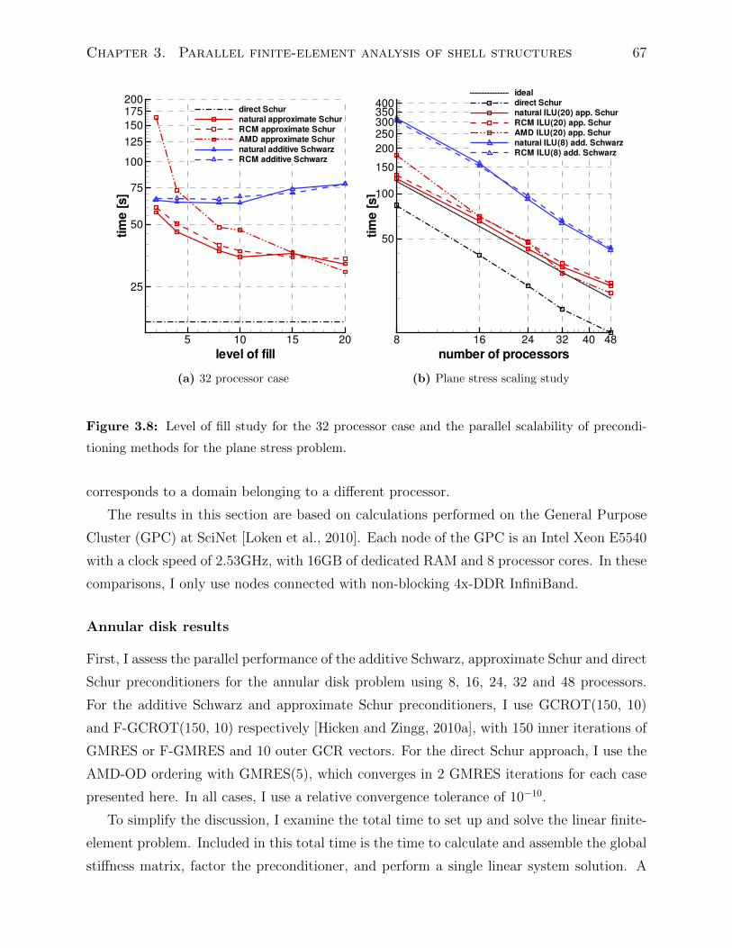
Chapter 3. Parallel finite-element analysis of shell structures 67
level of fill
time[s]
5 10 15 20
25
50
75
100
125
150
175
200direct Schur
natural approximate Schur
RCM approximate Schur
AMD approximate Schur
natural additive Schwarz
RCM additive Schwarz
(a) 32 processor case
number of processors
time[s]
8 16 24 32 40 48
50
100
150
200
250
300350400
ideal
direct Schur
natural ILU(20) app. Schur
RCM ILU(20) app. Schur
AMD ILU(20) app. Schur
natural ILU(8) add. Schwarz
RCM ILU(8) add. Schwarz
(b) Plane stress scaling study
Figure 3.8: Level of fill study for the 32 processor case and the parallel scalability of precondi-
tioning methods for the plane stress problem.
corresponds to a domain belonging to a different processor.
The results in this section are based on calculations performed on the General Purpose
Cluster (GPC) at SciNet [Loken et al., 2010]. Each node of the GPC is an Intel Xeon E5540
with a clock speed of 2.53GHz, with 16GB of dedicated RAM and 8 processor cores. In these
comparisons, I only use nodes connected with non-blocking 4x-DDR InfiniBand.
Annular disk results
First, I assess the parallel performance of the additive Schwarz, approximate Schur and direct
Schur preconditioners for the annular disk problem using 8, 16, 24, 32 and 48 processors.
For the additive Schwarz and approximate Schur preconditioners, I use GCROT(150, 10)
and F-GCROT(150, 10) respectively [Hicken and Zingg, 2010a], with 150 inner iterations of
GMRES or F-GMRES and 10 outer GCR vectors. For the direct Schur approach, I use the
AMD-OD ordering with GMRES(5), which converges in 2 GMRES iterations for each case
presented here. In all cases, I use a relative convergence tolerance of 10−10.
To simplify the discussion, I examine the total time to set up and solve the linear finite-
element problem. Included in this total time is the time to calculate and assemble the global
stiffness matrix, factor the preconditioner, and perform a single linear system solution. A
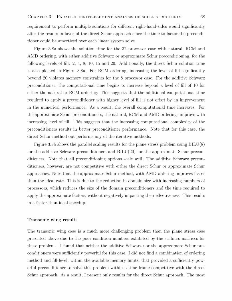
Chapter 3. Parallel finite-element analysis of shell structures 68
requirement to perform multiple solutions for different right-hand-sides would significantly
alter the results in favor of the direct Schur approach since the time to factor the precondi-
tioner could be amortized over each linear system solve.
Figure 3.8a shows the solution time for the 32 processor case with natural, RCM and
AMD ordering, with either additive Schwarz or approximate Schur preconditioning, for the
following levels of fill: 2, 4, 8, 10, 15 and 20. Additionally, the direct Schur solution time
is also plotted in Figure 3.8a. For RCM ordering, increasing the level of fill significantly
beyond 20 violates memory constraints for the 8 processor case. For the additive Schwarz
preconditioner, the computational time begins to increase beyond a level of fill of 10 for
either the natural or RCM ordering. This suggests that the additional computational time
required to apply a preconditioner with higher level of fill is not offset by an improvement
in the numerical performance. As a result, the overall computational time increases. For
the approximate Schur preconditioners, the natural, RCM and AMD orderings improve with
increasing level of fill. This suggests that the increasing computational complexity of the
preconditioners results in better preconditioner performance. Note that for this case, the
direct Schur method out-performs any of the iterative methods.
Figure 3.8b shows the parallel scaling results for the plane stress problem using BILU(8)
for the additive Schwarz preconditioners and BILU(20) for the approximate Schur precon-
ditioners. Note that all preconditioning options scale well. The additive Schwarz precon-
ditioners, however, are not competitive with either the direct Schur or approximate Schur
approaches. Note that the approximate Schur method, with AMD ordering improves faster
than the ideal rate. This is due to the reduction in domain size with increasing numbers of
processors, which reduces the size of the domain preconditioners and the time required to
apply the approximate factors, without negatively impacting their effectiveness. This results
in a faster-than-ideal speedup.
Transonic wing results
The transonic wing case is a much more challenging problem than the plane stress case
presented above due to the poor condition numbers exhibited by the stiffness matrices for
these problems. I found that neither the additive Schwarz nor the approximate Schur pre-
conditioners were sufficiently powerful for this case. I did not find a combination of ordering
method and fill-level, within the available memory limits, that provided a sufficiently pow-
erful preconditioner to solve this problem within a time frame competitive with the direct
Schur approach. As a result, I present only results for the direct Schur approach. The most
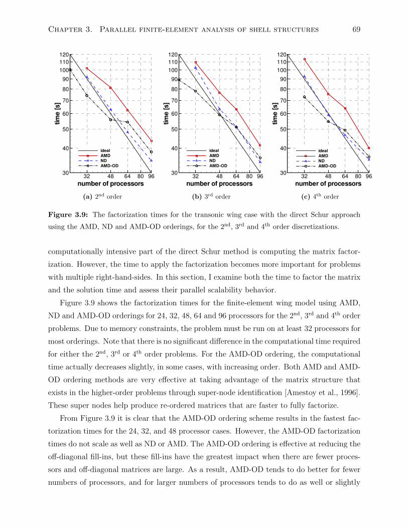
Chapter 3. Parallel finite-element analysis of shell structures 69
number of processors
time[s]
32 48 64 80 9630
40
50
60
70
80
90
100
110
120
ideal
AMD
ND
AMDOD
(a) 2nd order
number of processors
time[s]
32 48 64 80 9630
40
50
60
70
80
90
100
110
120
ideal
AMD
ND
AMDOD
(b) 3rd order
number of processors
time[s]
32 48 64 80 9630
40
50
60
70
80
90
100
110
120
ideal
AMD
ND
AMDOD
(c) 4th order
Figure 3.9: The factorization times for the transonic wing case with the direct Schur approach
using the AMD, ND and AMD-OD orderings, for the 2nd, 3rd and 4th order discretizations.
computationally intensive part of the direct Schur method is computing the matrix factor-
ization. However, the time to apply the factorization becomes more important for problems
with multiple right-hand-sides. In this section, I examine both the time to factor the matrix
and the solution time and assess their parallel scalability behavior.
Figure 3.9 shows the factorization times for the finite-element wing model using AMD,
ND and AMD-OD orderings for 24, 32, 48, 64 and 96 processors for the 2nd, 3rd and 4th order
problems. Due to memory constraints, the problem must be run on at least 32 processors for
most orderings. Note that there is no significant difference in the computational time required
for either the 2nd, 3rd or 4th order problems. For the AMD-OD ordering, the computational
time actually decreases slightly, in some cases, with increasing order. Both AMD and AMD-
OD ordering methods are very effective at taking advantage of the matrix structure that
exists in the higher-order problems through super-node identification [Amestoy et al., 1996].
These super nodes help produce re-ordered matrices that are faster to fully factorize.
From Figure 3.9 it is clear that the AMD-OD ordering scheme results in the fastest fac-
torization times for the 24, 32, and 48 processor cases. However, the AMD-OD factorization
times do not scale as well as ND or AMD. The AMD-OD ordering is effective at reducing the
off-diagonal fill-ins, but these fill-ins have the greatest impact when there are fewer proces-
sors and off-diagonal matrices are large. As a result, AMD-OD tends to do better for fewer
numbers of processors, and for larger numbers of processors tends to do as well or slightly
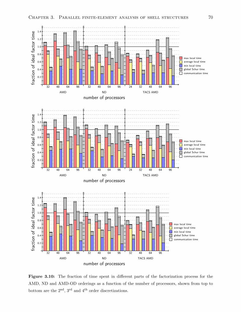
Chapter 3. Parallel finite-element analysis of shell structures 70
0.2
0.4
0.6
0.8
1.0
1.2
1.4
32 48 64 96 32 48 64 96 24 32 48 64 96
AMD ND TACS AMD
number of processors
fraction
ofidealfactor
time
max local time
average local time
min local time
global Schur time
communication time
0.2
0.4
0.6
0.8
1.0
1.2
1.4
32 48 64 96 32 48 64 96 24 32 48 64 96
AMD ND TACS AMD
number of processors
fraction
ofidealfactor
time
max local time
average local time
min local time
global Schur time
communication time
0.2
0.4
0.6
0.8
1.0
1.2
1.4
32 48 64 96 32 48 64 96 32 48 64 96
AMD ND TACS AMD
number of processors
fraction
ofidealfactor
time
max local time
average local time
min local time
global Schur time
communication time
Figure 3.10: The fraction of time spent in different parts of the factorization process for the
AMD, ND and AMD-OD orderings as a function of the number of processors, shown from top to
bottom are the 2nd, 3rd and 4th order discretizations.
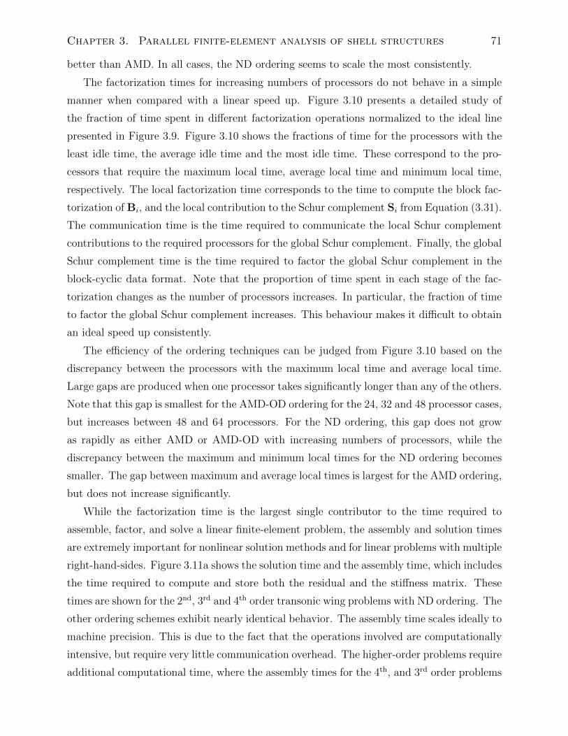
Chapter 3. Parallel finite-element analysis of shell structures 71
better than AMD. In all cases, the ND ordering seems to scale the most consistently.
The factorization times for increasing numbers of processors do not behave in a simple
manner when compared with a linear speed up. Figure 3.10 presents a detailed study of
the fraction of time spent in different factorization operations normalized to the ideal line
presented in Figure 3.9. Figure 3.10 shows the fractions of time for the processors with the
least idle time, the average idle time and the most idle time. These correspond to the pro-
cessors that require the maximum local time, average local time and minimum local time,
respectively. The local factorization time corresponds to the time to compute the block fac-
torization of Bi, and the local contribution to the Schur complement Si from Equation (3.31).
The communication time is the time required to communicate the local Schur complement
contributions to the required processors for the global Schur complement. Finally, the global
Schur complement time is the time required to factor the global Schur complement in the
block-cyclic data format. Note that the proportion of time spent in each stage of the fac-
torization changes as the number of processors increases. In particular, the fraction of time
to factor the global Schur complement increases. This behaviour makes it difficult to obtain
an ideal speed up consistently.
The efficiency of the ordering techniques can be judged from Figure 3.10 based on the
discrepancy between the processors with the maximum local time and average local time.
Large gaps are produced when one processor takes significantly longer than any of the others.
Note that this gap is smallest for the AMD-OD ordering for the 24, 32 and 48 processor cases,
but increases between 48 and 64 processors. For the ND ordering, this gap does not grow
as rapidly as either AMD or AMD-OD with increasing numbers of processors, while the
discrepancy between the maximum and minimum local times for the ND ordering becomes
smaller. The gap between maximum and average local times is largest for the AMD ordering,
but does not increase significantly.
While the factorization time is the largest single contributor to the time required to
assemble, factor, and solve a linear finite-element problem, the assembly and solution times
are extremely important for nonlinear solution methods and for linear problems with multiple
right-hand-sides. Figure 3.11a shows the solution time and the assembly time, which includes
the time required to compute and store both the residual and the stiffness matrix. These
times are shown for the 2nd, 3rd and 4th order transonic wing problems with ND ordering. The
other ordering schemes exhibit nearly identical behavior. The assembly time scales ideally to
machine precision. This is due to the fact that the operations involved are computationally
intensive, but require very little communication overhead. The higher-order problems require
additional computational time, where the assembly times for the 4th, and 3rd order problems
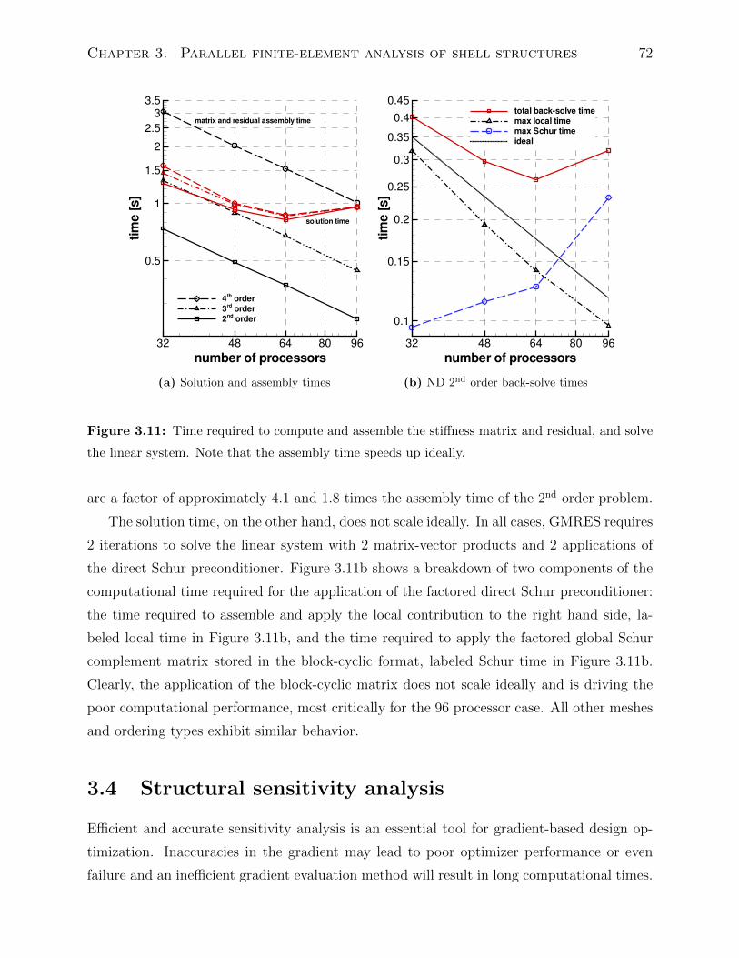
Chapter 3. Parallel finite-element analysis of shell structures 72
number of processors
time[s]
32 48 64 80 96
0.5
1
1.5
2
2.5
3
3.5
4thorder
3rdorder
2ndorder
solution time
matrix and residual assembly time
(a) Solution and assembly times
number of processors
time[s]
32 48 64 80 96
0.1
0.15
0.2
0.25
0.3
0.35
0.4
0.45total backsolve time
max local time
max Schur time
ideal
(b) ND 2nd order back-solve times
Figure 3.11: Time required to compute and assemble the stiffness matrix and residual, and solve
the linear system. Note that the assembly time speeds up ideally.
are a factor of approximately 4.1 and 1.8 times the assembly time of the 2nd order problem.
The solution time, on the other hand, does not scale ideally. In all cases, GMRES requires
2 iterations to solve the linear system with 2 matrix-vector products and 2 applications of
the direct Schur preconditioner. Figure 3.11b shows a breakdown of two components of the
computational time required for the application of the factored direct Schur preconditioner:
the time required to assemble and apply the local contribution to the right hand side, la-
beled local time in Figure 3.11b, and the time required to apply the factored global Schur
complement matrix stored in the block-cyclic format, labeled Schur time in Figure 3.11b.
Clearly, the application of the block-cyclic matrix does not scale ideally and is driving the
poor computational performance, most critically for the 96 processor case. All other meshes
and ordering types exhibit similar behavior.
3.4 Structural sensitivity analysis
Efficient and accurate sensitivity analysis is an essential tool for gradient-based design op-
timization. Inaccuracies in the gradient may lead to poor optimizer performance or even
failure and an inefficient gradient evaluation method will result in long computational times.
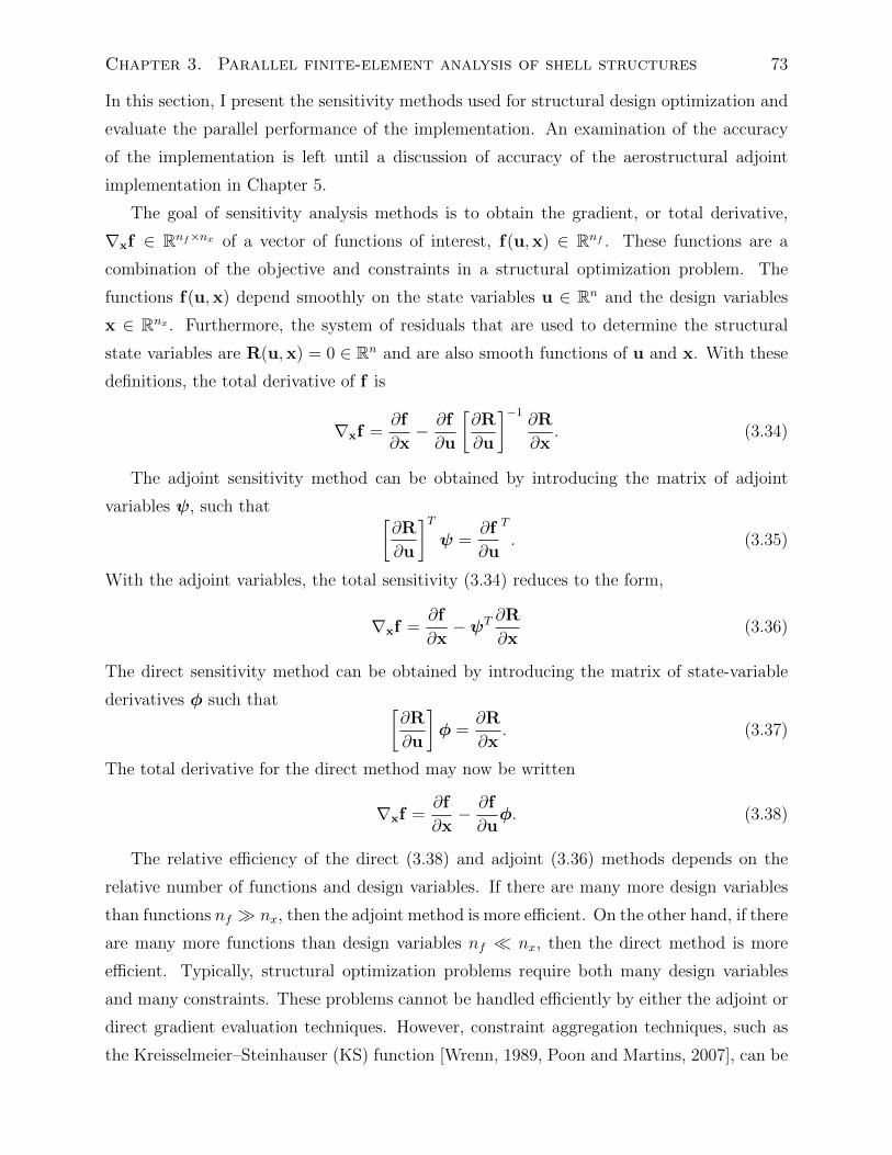
Chapter 3. Parallel finite-element analysis of shell structures 73
In this section, I present the sensitivity methods used for structural design optimization and
evaluate the parallel performance of the implementation. An examination of the accuracy
of the implementation is left until a discussion of accuracy of the aerostructural adjoint
implementation in Chapter 5.
The goal of sensitivity analysis methods is to obtain the gradient, or total derivative,
∇xf ∈ Rnf×nx of a vector of functions of interest, f(u,x) ∈ Rnf . These functions are a
combination of the objective and constraints in a structural optimization problem. The
functions f(u,x) depend smoothly on the state variables u ∈ Rn and the design variables
x ∈ Rnx . Furthermore, the system of residuals that are used to determine the structural
state variables are R(u,x) = 0 ∈ Rn and are also smooth functions of u and x. With these
definitions, the total derivative of f is
∇xf =∂f
∂x− ∂f
∂u
[∂R
∂u
]−1∂R
∂x. (3.34)
The adjoint sensitivity method can be obtained by introducing the matrix of adjoint
variables ψ, such that [∂R
∂u
]Tψ =
∂f
∂u
T
. (3.35)
With the adjoint variables, the total sensitivity (3.34) reduces to the form,
∇xf =∂f
∂x−ψT ∂R
∂x(3.36)
The direct sensitivity method can be obtained by introducing the matrix of state-variable
derivatives φ such that [∂R
∂u
]φ =
∂R
∂x. (3.37)
The total derivative for the direct method may now be written
∇xf =∂f
∂x− ∂f
∂uφ. (3.38)
The relative efficiency of the direct (3.38) and adjoint (3.36) methods depends on the
relative number of functions and design variables. If there are many more design variables
than functions nf nx, then the adjoint method is more efficient. On the other hand, if there
are many more functions than design variables nf nx, then the direct method is more
efficient. Typically, structural optimization problems require both many design variables
and many constraints. These problems cannot be handled efficiently by either the adjoint or
direct gradient evaluation techniques. However, constraint aggregation techniques, such as
the Kreisselmeier–Steinhauser (KS) function [Wrenn, 1989, Poon and Martins, 2007], can be
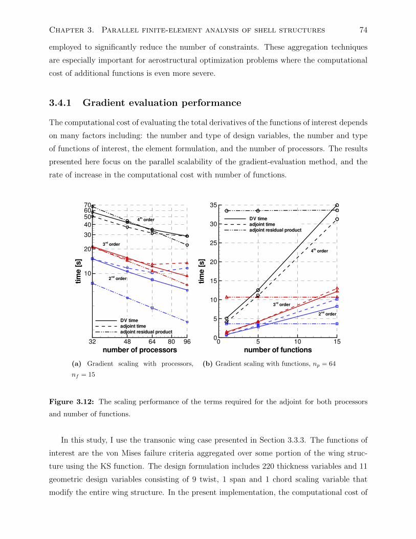
Chapter 3. Parallel finite-element analysis of shell structures 74
employed to significantly reduce the number of constraints. These aggregation techniques
are especially important for aerostructural optimization problems where the computational
cost of additional functions is even more severe.
3.4.1 Gradient evaluation performance
The computational cost of evaluating the total derivatives of the functions of interest depends
on many factors including: the number and type of design variables, the number and type
of functions of interest, the element formulation, and the number of processors. The results
presented here focus on the parallel scalability of the gradient-evaluation method, and the
rate of increase in the computational cost with number of functions.
number of processors
time[s]
32 48 64 80 96
10
20
30
40
50
6070
DV time
adjoint time
adjoint residual product
4thorder
3rdorder
2ndorder
(a) Gradient scaling with processors,
nf = 15
number of functions
time[s]
0 5 10 150
5
10
15
20
25
30
35
DV time
adjoint time
adjoint residual product
4thorder
3rdorder
2ndorder
(b) Gradient scaling with functions, np = 64
Figure 3.12: The scaling performance of the terms required for the adjoint for both processors
and number of functions.
In this study, I use the transonic wing case presented in Section 3.3.3. The functions of
interest are the von Mises failure criteria aggregated over some portion of the wing struc-
ture using the KS function. The design formulation includes 220 thickness variables and 11
geometric design variables consisting of 9 twist, 1 span and 1 chord scaling variable that
modify the entire wing structure. In the present implementation, the computational cost of
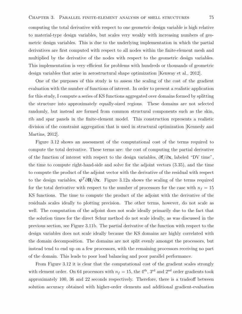
Chapter 3. Parallel finite-element analysis of shell structures 75
computing the total derivative with respect to one geometric design variable is high relative
to material-type design variables, but scales very weakly with increasing numbers of geo-
metric design variables. This is due to the underlying implementation in which the partial
derivatives are first computed with respect to all nodes within the finite-element mesh and
multiplied by the derivative of the nodes with respect to the geometric design variables.
This implementation is very efficient for problems with hundreds or thousands of geometric
design variables that arise in aerostructural shape optimization [Kenway et al., 2012].
One of the purposes of this study is to assess the scaling of the cost of the gradient
evaluation with the number of functions of interest. In order to present a realistic application
for this study, I compute a series of KS functions aggregated over domains formed by splitting
the structure into approximately equally-sized regions. These domains are not selected
randomly, but instead are formed from common structural components such as the skin,
rib and spar panels in the finite-element model. This construction represents a realistic
division of the constraint aggregation that is used in structural optimization [Kennedy and
Martins, 2012].
Figure 3.12 shows an assessment of the computational cost of the terms required to
compute the total derivative. These terms are: the cost of computing the partial derivative
of the function of interest with respect to the design variables, ∂f/∂x, labeled “DV time”,
the time to compute right-hand-side and solve for the adjoint vectors (3.35), and the time
to compute the product of the adjoint vector with the derivative of the residual with respect
to the design variables, ψT∂R/∂x. Figure 3.12a shows the scaling of the terms required
for the total derivative with respect to the number of processors for the case with nf = 15
KS functions. The time to compute the product of the adjoint with the derivative of the
residuals scales ideally to plotting precision. The other terms, however, do not scale as
well. The computation of the adjoint does not scale ideally primarily due to the fact that
the solution times for the direct Schur method do not scale ideally, as was discussed in the
previous section, see Figure 3.11b. The partial derivative of the function with respect to the
design variables does not scale ideally because the KS domains are highly correlated with
the domain decomposition. The domains are not split evenly amongst the processors, but
instead tend to end up on a few processors, with the remaining processors receiving no part
of the domain. This leads to poor load balancing and poor parallel performance.
From Figure 3.12 it is clear that the computational cost of the gradient scales strongly
with element order. On 64 processors with nf = 15, the 4th, 3rd and 2nd order gradients took
approximately 100, 36 and 22 seconds respectively. Therefore, there is a tradeoff between
solution accuracy obtained with higher-order elements and additional gradient-evaluation
Chapter 3. Parallel finite-element analysis of shell structures 76
costs for design optimization. Based on this analysis, and the frequent appearance of stress
concentrations in practical shell design problems that limit the asymptotic convergence rate,
I usually use 3rd order elements, which provide better stress resolution capability at no
additional analysis cost, with a slightly higher computation cost for the gradient-evaluation
compared to 2nd order elements.
3.5 Conclusions
In this chapter, I have presented the components of a framework for the parallel analysis and
gradient-based design optimization of thin shell structures. These components have been im-
plemented in a unified framework, called the Toolkit for the Analysis of Composite Structures
(TACS). In particular, I have presented a higher-order shell element formulation that enables
the accurate determination of the stress and strain distribution in thin shell structures. In
order to solve the linear systems resulting from the finite-element discretization, I presented
the additive Schwarz preconditioner, approximate Schur preconditioner and the direct Schur
method and I demonstrated that each of these methods exhibit good parallel scalability for
a plane stress problem, when used in conjunction with GCROT, F-GCROT or GMRES. Of
these methods, I demonstrated that the direct Schur approach required the least computa-
tional time to solve the resulting linear system. I also applied these solvers to a structural
model of a transonic wing case. For this case, the inexact preconditioners were inadequate
and only the direct Schur method provided a sufficiently powerful preconditioner. For the
transonic transport wing, I compared three ordering algorithms: AMD, ND and AMD-OD.
I demonstrated that the AMD-OD ordering was the fastest for problems with 24, 32, or 48
processors, while the ND ordering was fastest for the 64 or 96 processor cases. Furthermore,
I demonstrated that the solution times do not vary significantly with increasing element
order. Finally, I presented the implementation of a parallel gradient-evaluation technique
for the determination of derivatives of functions of interest. I examined the scalability of
the adjoint gradient-evaluation method with increasing processor count, increasing numbers
of functions and increasing element order. I demonstrated that the gradient computational
times increase significantly for higher-order elements. Therefore, there is a tradeoff between
higher-accuracy solutions obtained by increasing the element order, and computational time
for gradient-based optimization. When combined, the methods presented in this chapter en-
able efficient, parallel design optimization of complex thin shell structures used for aerospace
applications.
Chapter 4
Laminate parametrization
The parametrization of composite structures for design optimization is a challenging prob-
lem. Realistic structural design optimization problems require numerous manufacturing
constraints, which often include a restriction to select amongst a discrete set of available
ply angles. This discrete problem is not, in its most natural form, amenable to gradient-
based optimization. However, methods for nonlinear mixed-integer programming are almost
inevitably computationally expensive, especially for large numbers of design variables or
large design spaces. In this chapter, I present a laminate parametrization technique that
takes into account the discrete nature of some of the ply angle variables. In order to avoid
solving a large, nonlinear, mixed-integer program, I use a relaxation approach where the
original discrete problem is transformed into a continuous analogue of the original problem.
Gradient-based optimization can then be used to obtain solutions to the modified prob-
lem. To illustrate the effectiveness of the proposed laminate parametrization technique, I
present results from a series of structural optimization problems including design for min-
imum compliance, design for maximum critical end shortening and design problems with
strength criteria.
This chapter is structured as follows. In Section 4.1, I review the relevant literature
on laminate parametrization techniques. In Section 4.2, I describe the proposed laminate
parametrization technique and present a method for predicting material failure within the
context of the laminate parametrization. In Section 4.3, I describe additional manufacturing
constraints that may be required for certain laminate design problems. In Section 4.4, I
present a series of optimization results, including a compliance minimization study and a
stiffened panel buckling optimization. Finally, in Section 4.5, I present an application of
the proposed laminate parametrization technique to the lamination sequence design of a
composite wing-box. Most of the material in this chapter was published in Kennedy and
77
Chapter 4. Laminate parametrization 78
Martins [2012].
4.1 Literature review
Laminate parametrization techniques generally fall into two categories: direct parametriza-
tions that provide an explicit description of the physical laminate, and indirect parametriza-
tions in which intermediate variables are employed and the lamination sequence is only
available in a post-processing calculation. There are difficulties with using either of these
approaches. Direct techniques often introduce many local minima in the design space, while
indirect methods make it difficult to impose manufacturing constraints on the physical con-
struction of the laminate.
The use of ply angle variables and the integer number of plies is the most direct parametriza-
tion of a lamination sequence. However, this type of parametrization suffers from several
drawbacks. First, the combination of the ply-angle variables and the integral number of plies
necessitates mixed-integer programming techniques [Haftka and Gurdal, 1992]. Second, it
is well known that the parametrization using ply-angle variables, for fixed number of plies,
introduces many local minima [Stegmann and Lund, 2005]. Nevertheless, researchers have
developed various techniques to address these issues. For instance, Bruyneel and Fleury
[2002] and Bruyneel [2006] developed an effective, gradient-base optimization approach for
composite structures parametrized with ply angles, for stiffness, strength and weight design
criteria. However, these parametrizations still do not address manufacturing constraints that
limit available ply angles to a discrete set.
The constitutive matrices in classical lamination theory (CLT) and in first-order shear
deformation theory (FSDT) can be expressed in terms of the material invariants and 12
integrals of trigonometric functions of the ply-angle distribution through the thickness of the
laminate. When these integrals are treated as variables, rather than explicit functions of the
lamination sequence, they are referred to as the lamination parameters [Tsai and Pagano,
1968]. Due to the relationship between these integrals, not all combinations of the lamina-
tion parameters represent physically realizable laminates. As a result, constraints must be
imposed to restrict the values of the parameters to a physically-realizable domain [Hammer
et al., 1997]. An expression for the full feasible space of lamination parameters is not known
explicitly, so often a subset of the variables are used for design.
Lamination parameters have often been used as a parametrization for stiffness and buck-
ling design. Fukunaga and Vanderplaats [1991] performed buckling optimization of cylindri-
cal shells with symmetric, orthotropic laminates using two in-plane and two flexural lami-
Chapter 4. Laminate parametrization 79
nation parameters. Fukunaga and Vanderplaats also solved the inverse problem to obtain
the explicit lamination sequences. Later, Fukunaga and Sekine [1992] performed stiffness
design of laminates and obtained explicit expressions for the feasible space of symmetric
laminates. Miki and Sugiyama [1993] used lamination parameters for the compliance and
buckling design of symmetric, orthotropic laminates. Hammer et al. [1997] presented an
extensive theoretical development of the mathematical properties of lamination parameters
and used them for compliance design of symmetric laminates subject to single and multiple
loading conditions. Liu et al. [2004] designed simply supported symmetric plates for buckling
using lamination parameters. They imposed a constraint on the number of plies at 0o, ±45o
and 90o and mapped these constraints into a hexagonal region in the lamination parameter
space.
Other authors have extended the use of the lamination parameters beyond stiffness and
buckling design applications. Foldager et al. [1998], used lamination parameters to avoid
local minima while performing compliance minimization using ply angle design variables.
IJsselmuiden et al. [2008] performed strength-based design studies using lamination parame-
ters by incorporating the Tsai–Wu failure criteria [Jones, 1996] into the lamination parameter
space to obtain a conservative failure envelope.
While lamination parameter based parametrizations have been used effectively in many
applications, one of the primary disadvantages of this approach is that it does not provide a
direct description of the laminate construction. This makes it difficult to impose constraints
on ply angles that may be required due to manufacturing considerations. Furthermore,
lamination parameters, by themselves, do not provide a lamination sequence and therefore
can only be viewed as an intermediate design result.
Often, for manufacturing reasons, the ply angles available to the designer are restricted to
a discrete set of options such as 0o, ±45o and 90o. With this restriction, the laminate sequence
design problem becomes a mixed-integer programming problem. Various authors have used
either mixed-integer programming techniques or genetic algorithms (GAs) to solve laminate
stacking sequence problems poised with a discrete set of ply angles. Haftka and Walsh [1992]
formulated the buckling-load maximization of a simply supported plate, with and without
ply contiguity constraints, as a linear integer programming problem and obtained global
optimum designs using a branch and bound algorithm. Le Riche and Haftka [1993] performed
buckling-load maximization of a simply-supported plate with strength and ply contiguity
constraints using a GA. Later, Liu et al. [2000b] performed buckling-load maximization for a
simply supported plate with a constraint on the number of plies at each available angle using
a permutation GA. More recently, Adams et al. [2004] used a GA for a realistic composite
Chapter 4. Laminate parametrization 80
wing-box design problem with a thick guide laminate and blended plies.
The main advantage of using GAs for laminate design problems, is that they have the
ability to work with integer variables directly. Furthermore, GAs are more likely to get close
to the global optimum, regardless of whether the underlying design space is multi-modal
or discontinuous. However, GAs often require several orders of magnitude more function
evaluations than gradient-based approaches, especially for large design spaces. This property
of GAs is especially problematic when employing high-fidelity computational methods that
require significant computational time for a single analysis.
Discrete material optimization (DMO) approaches can be used as either multi-material
or laminate sequence parametrizations. DMO was first proposed by Stegmann and Lund
[2005] based on the work of Sigmund and Torquato [1997]. In the DMO approach, applied
to laminate design, the stiffness contribution from every discrete ply-angle, in each layer
is multiplied by a weighting function. Instead of using a linear interpolant, a SIMP-type
penalization is employed such that the stiffness-to-weight ratio of intermediate designs are
less favorable. Stegmann and Lund [2005] and later Lund [2009] applied the DMO approach
to the compliance and buckling optimization of composite shells.
Other authors have extended SIMP and DMO-type approaches. Bruyneel [2011] de-
veloped an approach, similar to DMO, for selection amongst a discrete set of four plies
using bilinear shape function weights. This approach, called the shape function with penal-
ization (SFP) parametrization, reduces the number of design variables compared to DMO
approaches. Bruyneel et al. [2011] extended the SFP approach to material selection amongst
different numbers of plies by using different interpolation functions. Using a different ap-
proach, Hvejsel et al. [2011] developed a technique for laminate parametrization that, in a
similar manner to DMO, uses a weighted sum of contributions to the stiffness. In a depar-
ture from the DMO approach, they employed an exact, quadratic concave penalty constraint
function, first used by Borrvall and Petersson [2001], to force the design towards a discrete
solution. They demonstrated their approach on a series of compliance minimization prob-
lems.
One of the main advantages of DMO and DMO-type parametrizations, is that they can be
used with gradient-based optimization techniques. As a result, DMO parametrizations can
be used on very large design problems for which gradient-free methods, such as GAs, would
be ineffective. However, DMO and SIMP-type approaches may only produce a local optimum
solution [Stolpe and Svanberg, 2001b,a]. Furthermore, DMO and DMO-type approaches may
fail to converge to a fully discrete design, especially for objectives other than compliance and
it may be difficult to assess the merits of an intermediate solution.
Chapter 4. Laminate parametrization 81
The laminate parametrization I present below is a direct parametrization that provides
an explicit description of the lamination sequence. The proposed approach is a continuous
regularization of a discrete mixed-integer laminate formulation. Similar to the DMO ap-
proach of Hvejsel et al. [2011], I interpolate between a discrete set of possible angles using
a linear combination of material stiffnesses. In a departure from previous work, I add an
exact `1 penalty function to the objective function to force the design towards a discrete
solution. The `1 penalty function is not differentiable, so I propose an elastic programming
approach that produces the effect of the `1 penalty function in a differentiable manner within
the optimization problem. Simplifications to the penalization can be made if certain linear
constraints are satisfied exactly at all optimization iterations. Compared to DMO-type ap-
proaches, the present approach is more effective at obtaining fully converged designs due to
the exact `1 peanlization. In a departure from previous papers on DMO-type methods, I
also introduce additional complementarity constraints on the ply angles that may arise due
to manufacturing considerations. These complementarity constraints are handled through
a regularization technique proposed by Scholtes [2001]. I apply the proposed approach to
several structural optimization problems of increasing complexity, including a compliance
minimization problem, a stiffened-panel design for buckling and a wing-box sizing and lam-
ination sequence design study.
4.2 The proposed laminate parametrization
In the following laminate parametrization technique, I consider a structure that is split into
a series of M design segments. Each design segment is composed of a single laminate with N
layers, where in each layer, the ply angles must be selected from a discrete set of K allowable
angles, Θ = θ1, θ2, . . . , θK. For ease of presentation, the number of layers and number of
allowable ply angles is fixed to N and K for all segments. This restriction, however, is not
required, and in general, the number of plies and number of available ply angles may vary
between design segments.
Each design segment of the structure is modeled using first-order shear deformation
theory (FSDT), where the in-plane, bending-stretching coupling, bending and transverse
shear constitutive matrices are: A(i), B(i), D(i), A(i)s . Note that the superscript i indexes
the ith design segment, where i = 1, . . . ,M .
In the following description, I first outline the proposed laminate parametrization using
a mixed-integer formulation and then proceed to relax the discrete problem to a continuous
formulation. In the proposed parametrization technique, the constitutive matrices, A(i), B(i),
Chapter 4. Laminate parametrization 82
D(i), A(i)s , are expressed in terms of a series of discrete ply-identity variables ξijk ∈ 0, 1:
A(i) =N∑j=1
(hij+1 − hij)K∑k=1
ξijkQ(θk), B(i) =N∑j=1
1
2(h2
ij+1 − h2ij)
K∑k=1
ξijkQ(θk),
D(i) =N∑j=1
1
3(h3
ij+1 − h3ij)
K∑k=1
ξijkQ(θk), As(i) = κ
N∑j=1
(hij+1 − hij)K∑k=1
ξijkQs(θk),
(4.1)
where there are N plies in the laminate, Q(θ) and Qs(θ) are the laminae in-plane and shear
stiffnesses in the global coordinate system [Jones, 1996], and hij are the through-thickness
coordinate of the jth layer-interface in the ith design segment.
An active ply-identity variable, ξijk = 1, indicates that the kth ply angle, θk, in the jth
layer of the ith design segment has been selected. To avoid selecting multiple ply angles in
the same layer, it is necessary to impose the following constraint:
K∑k=1
ξijk = 1, i = 1, . . . , N, j = 1, . . . ,M. (4.2)
Note that this discrete formulation is identical to the mixed-integer approach of Haftka and
Walsh [1992]. Equation (4.2) ensures that one and only one ply is active in each layer, thus
ξijp = 1 for some p, while ξijk = 0 for k 6= p.
The number of possible designs increases rapidly as the number of ply angles, layers and
design segments increase. Evaluating all possible designs quickly becomes computationally
intractable as there are KMN possible combinations.
Instead of using the discrete variables ξijk ∈ 0, 1, I relax the mixed-integer problem
and use continuous variables, written as: xijk ∈ [0, 1]. The continuous design variables, xijk,
are called the ply selection variables, and continuous designs that satisfy xijk ∈ 0, 1 are
called 0-1 points. The stiffness can now be expressed in terms of the continuous ply selection
variables as follows:
A(i) =N∑j=1
(hij+1 − hij)K∑k=1
xPijkQ(θk), B(i) =N∑j=1
1
2(h2
ij+1 − h2ij)
K∑k=1
xPijkQ(θk),
D(i) =N∑j=1
1
3(h3
ij+1 − h3ij)
K∑k=1
xPijkQ(θk), As(i) = κ
N∑j=1
(hij+1 − hij)K∑k=1
xPijkQs(θk),
(4.3)
where xijk are continuous over the interval [0, 1]. Note that the SIMP parameter P has
been introduced as an exponent on the continuous ply identity variables. The purpose of
the parameter P is to penalize the stiffness of intermediate designs such that 0-1 points have
more favorable stiffness-to-weight ratios. Often, a continuation approach is employed where
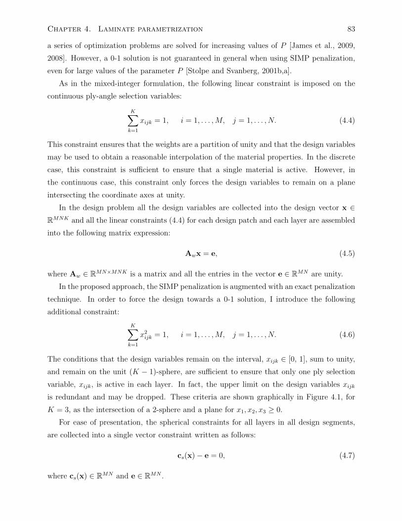
Chapter 4. Laminate parametrization 83
a series of optimization problems are solved for increasing values of P [James et al., 2009,
2008]. However, a 0-1 solution is not guaranteed in general when using SIMP penalization,
even for large values of the parameter P [Stolpe and Svanberg, 2001b,a].
As in the mixed-integer formulation, the following linear constraint is imposed on the
continuous ply-angle selection variables:
K∑k=1
xijk = 1, i = 1, . . . ,M, j = 1, . . . , N. (4.4)
This constraint ensures that the weights are a partition of unity and that the design variables
may be used to obtain a reasonable interpolation of the material properties. In the discrete
case, this constraint is sufficient to ensure that a single material is active. However, in
the continuous case, this constraint only forces the design variables to remain on a plane
intersecting the coordinate axes at unity.
In the design problem all the design variables are collected into the design vector x ∈RMNK and all the linear constraints (4.4) for each design patch and each layer are assembled
into the following matrix expression:
Awx = e, (4.5)
where Aw ∈ RMN×MNK is a matrix and all the entries in the vector e ∈ RMN are unity.
In the proposed approach, the SIMP penalization is augmented with an exact penalization
technique. In order to force the design towards a 0-1 solution, I introduce the following
additional constraint:
K∑k=1
x2ijk = 1, i = 1, . . . ,M, j = 1, . . . , N. (4.6)
The conditions that the design variables remain on the interval, xijk ∈ [0, 1], sum to unity,
and remain on the unit (K − 1)-sphere, are sufficient to ensure that only one ply selection
variable, xijk, is active in each layer. In fact, the upper limit on the design variables xijk
is redundant and may be dropped. These criteria are shown graphically in Figure 4.1, for
K = 3, as the intersection of a 2-sphere and a plane for x1, x2, x3 ≥ 0.
For ease of presentation, the spherical constraints for all layers in all design segments,
are collected into a single vector constraint written as follows:
cs(x)− e = 0, (4.7)
where cs(x) ∈ RMN and e ∈ RMN .
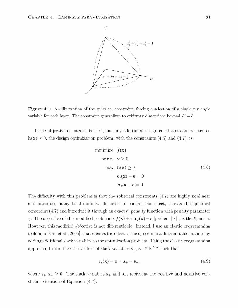
Chapter 4. Laminate parametrization 84
x1
x2
x3
x21 + x22 + x23 = 1
x1 + x2 + x3 = 1
Figure 4.1: An illustration of the spherical constraint, forcing a selection of a single ply angle
variable for each layer. The constraint generalizes to arbitrary dimensions beyond K = 3.
If the objective of interest is f(x), and any additional design constraints are written as
h(x) ≥ 0, the design optimization problem, with the constraints (4.5) and (4.7), is:
minimize f(x)
w.r.t. x ≥ 0
s.t. h(x) ≥ 0
cs(x)− e = 0
Awx− e = 0
(4.8)
The difficulty with this problem is that the spherical constraints (4.7) are highly nonlinear
and introduce many local minima. In order to control this effect, I relax the spherical
constraint (4.7) and introduce it through an exact `1 penalty function with penalty parameter
γ. The objective of this modified problem is f(x)+γ||cs(x)−e||1 where || · ||1 is the `1 norm.
However, this modified objective is not differentiable. Instead, I use an elastic programming
technique [Gill et al., 2005], that creates the effect of the `1 norm in a differentiable manner by
adding additional slack variables to the optimization problem. Using the elastic programming
approach, I introduce the vectors of slack variables s+, s− ∈ RMN such that
cs(x)− e = s+ − s−, (4.9)
where s+, s− ≥ 0. The slack variables s+ and s−, represent the positive and negative con-
straint violation of Equation (4.7).
Chapter 4. Laminate parametrization 85
The modified optimization problem then becomes:
minimize f(x) + γeT (s+ + s−)
w.r.t. x, s+, s− ≥ 0
s.t. h(x) ≥ 0
cs(x)− e = s+ − s−
Awx− e = 0
(4.10)
where the parameter γ > 0 is a penalty parameter. For a feasible problem, with a sufficiently
large, but finite value of γ, Problem (4.10) admits solutions, x∗, s∗+ = s∗− = 0, that are also
solutions to Problem (4.8). However, as γ → 0, Problem (4.10) admits solutions that are not
solutions to Problem (4.8) and do not satisfy the 0-1 criteria. To address this problem, I solve
the `1 penalized optimization problem (4.10) for increasing values of penalty parameter. For
small γ, this will allow greater freedom in exploring the design space, but with increasing γ,
the infeasibility measure ||cs(x)− e||1 will decrease.
A further simplification of Problem (4.10) can be achieved when the summation con-
straints (4.5) are satisfied exactly at every iteration. Starting from Equation (4.5), the sum
of the squared design variables must be less than one, i.e.
1 =
(K∑k=1
xijk
)2
≥K∑k=1
x2ijk.
As a result, when the linear constraint (4.5) is satisfied exactly, the constraint violation of
Equation (4.7) is negative, i.e. cs(x) − e ≤ 0. Therefore, the values of the slacks at the
solution are:
s∗+ = 0,
s∗− = e− cs(x∗).
This result can also be observed geometrically. Whenever the design lies on the plane, the
distance from the plane to the sphere is strictly positive, unless it is at a 0-1 point when the
normal distance is precisely zero, see Figure 4.1. Using this result, the optimization problem
Opt(γ), can now be written as follows:
minimize f(x) + γeT (e− cs(x))
w.r.t. x ≥ 0
s.t. h(x) ≥ 0
Awx ≡ e
(4.11)
Chapter 4. Laminate parametrization 86
where the final constraint is written as Awx ≡ e to indicate that it is satisfied at every
iteration.
I use a continuation approach and solve Opt(γn) for a sequence of increasing γn, starting
each subsequent optimization problem from the previous solution. In this work, I use the
sequential quadratic optimization code SNOPT [Gill et al., 2005], through the Python-based
wrapper in the optimization package pyOpt [Perez et al., 2012]. SNOPT is designed to
satisfy all the linear constraints exactly at every iteration.
4.2.1 Failure prediction
The prediction of structural failure is a critical aspect of preliminary structural design. In
this work, I employ a single conservative failure envelope that can be used to ensure that no
material occurs within the laminate. Note that it is also possible to construct a layer-wise
failure envelope within the context of this parametrization [Kennedy and Martins, 2012].
In this work, I use the Tsai–Wu failure criterion [Jones, 1996] to test if the lamina stresses
are within the failure envelope, written as
F (σ) ≤ 1. (4.12)
In practice, any failure criterion that takes the form of Equation (4.12) could be used.
To construct the overall laminate failure envelope, I apply the failure criteria at all
angles θk ∈ Θ, at the upper and lower surfaces of the laminate. Instead of applying each of
these criteria independently, I aggregate them into a single function using a Kreisselmeier–
Steinhauser (KS) aggregation technique [Wrenn, 1989]. This provides a conservative failure
envelope, but does not account for the variation of ply angles within the laminate. This
conservative failure envelope can be written as follows:
F(i)KS = KS(F (σ(p)), ρ) ≤ 1, (4.13)
where the aggregation takes place over the range p = 1, . . . , 2K. Here, σ(2k−1) and σ(2k)
are the laminae stresses at the angle θk on the top and bottom surfaces respectively. The
function KS( · , ρ) is the KS aggregation function with parameter ρ. Equation (4.13) pro-
vides a conservative failure envelope in the sense that when the laminate stresses are within
the envelope, all laminae within the layup are within the failure envelope represented by
Equation (4.12).
Chapter 4. Laminate parametrization 87
4.3 Adjacency constraints
In this section, I introduce a new constraint formulation that is designed to enforce additional
manufacturing requirements on the stacking sequence. This constraint restricts the allowable
ply angles in one layer, based on which ply angle is active in an adjacent layer. Since these
constraints are always imposed between adjacent layers, I call them adjacency constraints.
It may be necessary to impose adjacency constraints on a lamination sequence to prevent
large changes in the ply angles between layers, or to prevent repeated layers at the same ply
angle. The implementation of this type of adjacency constraint is described below.
Without loss of generality, consider first layer, j = 1, of the design segments, i = 1 and
i = 2, with design variables x11k and x21p respectively. If the design variable x11k is active
at the solution, then the purpose of the adjacency constraint is to restrict available choices
in the next design segment to some reduced set of options. Given that the kth-ply is active,
the set of design options that cannot be used in the adjacent segment is given by the set of
design variable indices Ik. Using the set Ik, this type of adjacency constraint can be imposed
as follows:
x11kx21p ≤ 0, k = 1, . . . , K,
p ∈ Ik.(4.14)
This type of constraint, in combination with the condition xijk ≥ 0, is known as a comple-
mentarity constraint [Scheel and Scholtes, 2000, Coulibaly and Orban, 2012]. The less-than
condition is used to conform to a standard complementarity constraint formulation. Un-
fortunately, complementarity constraints violate conventional constraint qualifications such
as the Mangasarian–Fromovitz constraint qualification (MFCQ) or the linear independence
constraint qualification (LICQ) [Nocedal and Wright, 1999, chap. 12]. As a result, these
types of constraints do not admit Lagrange multipliers at the solution and gradient-based
optimizers may encounter difficulties [Scheel and Scholtes, 2000, Scholtes, 2001, Coulibaly
and Orban, 2012].
Instead of using the complementarity constraint (4.14) directly, I use a regularization of
the constraint due to Scholtes [2001]. In this regularization technique, the original comple-
mentarity constraint is perturbed in the following manner:
x11kx21p ≤ τ, k = 1, . . . , K,
p ∈ Ik,(4.15)
for τ > 0. In the approach of Scholtes [2001], a series of optimization problems are then solved
for decreasing values of τ using a conventional SQP optimizer, starting each new problem
Chapter 4. Laminate parametrization 88
from the previous solution. This series of perturbed problems converges to a solution of the
original problem with some conditions on the linear independence of the constraint gradients
excluding the complementarity constraints [Scholtes, 2001].
In this work, I consider three options for the set of indices Ik. In the first case, the index
set Ik is constructed so that the plies may only shift L selections between adjacent layers.
In this case, the index set, Ik, is defined as follows:
Ik = 1, 2, . . . , K \ k − L, . . . , k + L. (4.16)
In the second case, the design selections are allowed to wrap around. For instance, if the
ply selection variable x111 is active, then x211 through x21L, as well as, x21N through x21(N−L)
could be active as well. In this case the index set is defined as:
Ik =
k ≤ L k + L+ 1, . . . , K + k − L− 1k ≥ K − L k −K + L+ 1, . . . , k − L− 1otherwise 1, 2, . . . , K \ k − L, . . . , k + L
. (4.17)
The final option is that once a design is active in one layer, it may not be active in the
second layer. In this case, the index set is defined as follows:
Ik = k. (4.18)
The total number of adjacency constraints can be reduced by combining groups of the
constraints (4.15) into a single equivalent constraint. In this work, I use the equivalent
constraint:
x11k
∑p∈Ik
x21p ≤ τ, k = 1, . . . , K. (4.19)
For ease of presentation, all of the grouped adjacency constraints (4.19) are written in the
following form:
d(x) ≤ τ, (4.20)
where d ∈ Rna , where na is the number of adjacency constraints in the form of Equa-
tion (4.19).
The original optimization problem (4.11) with the additional adjacency constraints as
Opt′(γ, τ), can be written as follows:
min f(x) + γeT (e− cs(x))
w.r.t. x ≥ 0
s.t. h(x) ≥ 0
d(x) ≤ τ
Awx ≡ e
(4.21)
Chapter 4. Laminate parametrization 89
The optimization problem Opt′(γn, τn) must be solved for a sequence γn, τn, with non-
decreasing γn and non-increasing τn.
4.3.1 Avoiding intermediate designs
The penalization approach presented in Section 4.2 ensures that for sufficiently large γ,
solutions to the optimization problem with the full set of spherical constraints (4.8), are also
solutions to the optimization problem (4.11). However, the converse is not true. That is,
local optima of the modified `1 penalty problem (4.11) may not be solutions to the original
problem (4.8), even for large values of γ. For optimization problems with certain constraints,
the sequence of solutions to Opt(γn) may converge to a solution for which ||cs(x∗n)−e||1 6= 0
even for large γn. This is a local minima since any feasible, 0-1 point, xf , with ||cs(xf )−e||1 =
0, has an objective value, f(xf ), lower than the penalized objective, f(x∗n)+γn||cs(x∗n)−e||1,
for a sufficiently large value of γn, even if f(x∗n) < f(xf ).
In practice, I have found that Opt(γn) may fail to converge to a 0-1 solution for problems
in which additional constraints are imposed on the ply selection variables. These additional
constraints impose conditions such that any feasible path away from the local solution yields
a higher value of the penalized objective. As a result, the continuation sequence does not
move away from the local minima and the solution does not proceed to a 0-1 point. To obtain
a 0-1 solution, in these cases, I impose an additional constraint which forces the optimum
away from the local minima. For each ply, I add the following complementarity constraint:
K−1∑k=1
xijk
K∑p=k+1
xijp ≤ τ, i = 1, . . . ,M, j = 1, . . . , N.
Note that this constraint is only imposed after a local minima has been detected. This
constraint ensures that as τ decreases, only a single ply selection variable will be non-zero
in each layer. However, by itself, this constraint does not force the design towards a 0-1
solution. For ease of presentation, I collect these constraints for each ply, in every design
segment, into the following vector of constraints:
g(x) ≤ τ, (4.22)
where g(x) ∈ RMN . As τ → 0, points at which more than one ply selection variable is
non-zero will become infeasible. While it would be possible to include this constraint for all
optimization problems, I have found that optimization problems with the constraint (4.22)
tend to require more function and gradient evaluations. As a result, I only include this
complementarity constraint once a local minima with ||cs(x∗n)− e||1 6= 0 is detected.
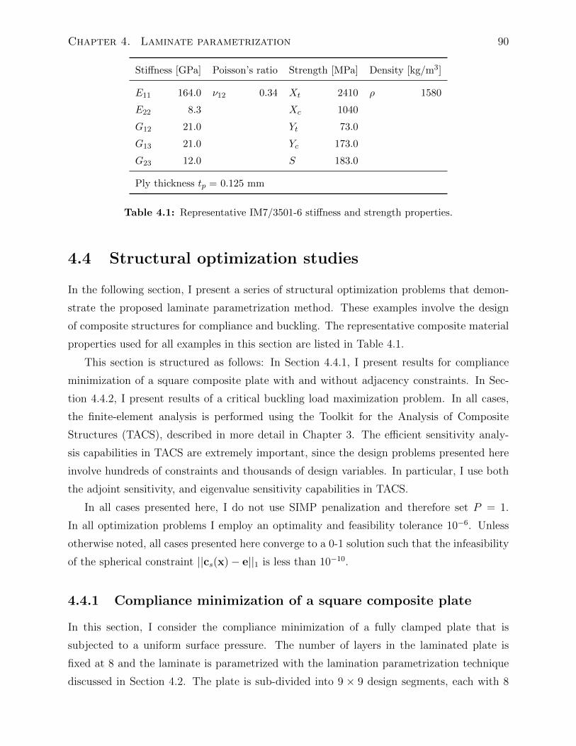
Chapter 4. Laminate parametrization 90
Stiffness [GPa] Poisson’s ratio Strength [MPa] Density [kg/m3]
E11 164.0 ν12 0.34 Xt 2410 ρ 1580
E22 8.3 Xc 1040
G12 21.0 Yt 73.0
G13 21.0 Yc 173.0
G23 12.0 S 183.0
Ply thickness tp = 0.125 mm
Table 4.1: Representative IM7/3501-6 stiffness and strength properties.
4.4 Structural optimization studies
In the following section, I present a series of structural optimization problems that demon-
strate the proposed laminate parametrization method. These examples involve the design
of composite structures for compliance and buckling. The representative composite material
properties used for all examples in this section are listed in Table 4.1.
This section is structured as follows: In Section 4.4.1, I present results for compliance
minimization of a square composite plate with and without adjacency constraints. In Sec-
tion 4.4.2, I present results of a critical buckling load maximization problem. In all cases,
the finite-element analysis is performed using the Toolkit for the Analysis of Composite
Structures (TACS), described in more detail in Chapter 3. The efficient sensitivity analy-
sis capabilities in TACS are extremely important, since the design problems presented here
involve hundreds of constraints and thousands of design variables. In particular, I use both
the adjoint sensitivity, and eigenvalue sensitivity capabilities in TACS.
In all cases presented here, I do not use SIMP penalization and therefore set P = 1.
In all optimization problems I employ an optimality and feasibility tolerance 10−6. Unless
otherwise noted, all cases presented here converge to a 0-1 solution such that the infeasibility
of the spherical constraint ||cs(x)− e||1 is less than 10−10.
4.4.1 Compliance minimization of a square composite plate
In this section, I consider the compliance minimization of a fully clamped plate that is
subjected to a uniform surface pressure. The number of layers in the laminated plate is
fixed at 8 and the laminate is parametrized with the lamination parametrization technique
discussed in Section 4.2. The plate is sub-divided into 9 × 9 design segments, each with 8
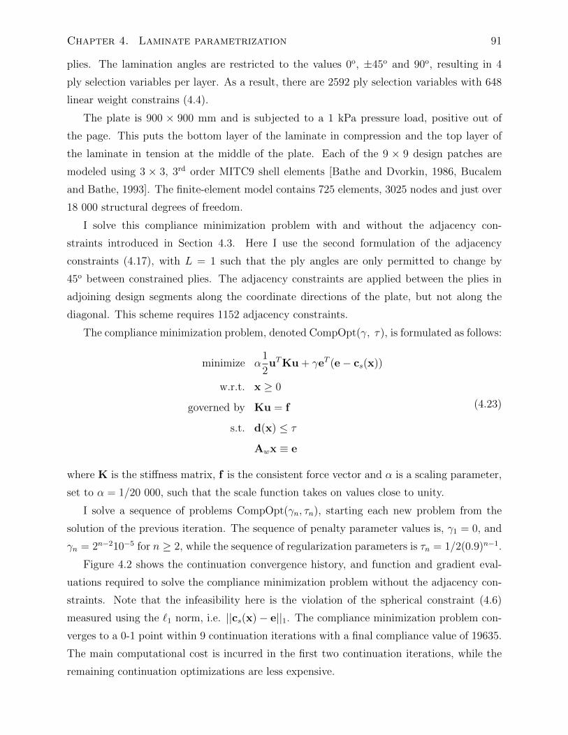
Chapter 4. Laminate parametrization 91
plies. The lamination angles are restricted to the values 0o, ±45o and 90o, resulting in 4
ply selection variables per layer. As a result, there are 2592 ply selection variables with 648
linear weight constrains (4.4).
The plate is 900 × 900 mm and is subjected to a 1 kPa pressure load, positive out of
the page. This puts the bottom layer of the laminate in compression and the top layer of
the laminate in tension at the middle of the plate. Each of the 9 × 9 design patches are
modeled using 3 × 3, 3rd order MITC9 shell elements [Bathe and Dvorkin, 1986, Bucalem
and Bathe, 1993]. The finite-element model contains 725 elements, 3025 nodes and just over
18 000 structural degrees of freedom.
I solve this compliance minimization problem with and without the adjacency con-
straints introduced in Section 4.3. Here I use the second formulation of the adjacency
constraints (4.17), with L = 1 such that the ply angles are only permitted to change by
45o between constrained plies. The adjacency constraints are applied between the plies in
adjoining design segments along the coordinate directions of the plate, but not along the
diagonal. This scheme requires 1152 adjacency constraints.
The compliance minimization problem, denoted CompOpt(γ, τ), is formulated as follows:
minimize α1
2uTKu + γeT (e− cs(x))
w.r.t. x ≥ 0
governed by Ku = f
s.t. d(x) ≤ τ
Awx ≡ e
(4.23)
where K is the stiffness matrix, f is the consistent force vector and α is a scaling parameter,
set to α = 1/20 000, such that the scale function takes on values close to unity.
I solve a sequence of problems CompOpt(γn, τn), starting each new problem from the
solution of the previous iteration. The sequence of penalty parameter values is, γ1 = 0, and
γn = 2n−210−5 for n ≥ 2, while the sequence of regularization parameters is τn = 1/2(0.9)n−1.
Figure 4.2 shows the continuation convergence history, and function and gradient eval-
uations required to solve the compliance minimization problem without the adjacency con-
straints. Note that the infeasibility here is the violation of the spherical constraint (4.6)
measured using the `1 norm, i.e. ||cs(x)− e||1. The compliance minimization problem con-
verges to a 0-1 point within 9 continuation iterations with a final compliance value of 19635.
The main computational cost is incurred in the first two continuation iterations, while the
remaining continuation optimizations are less expensive.
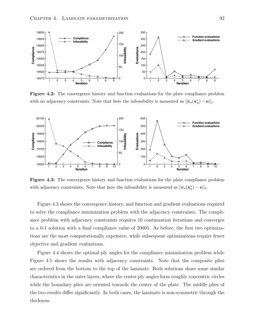
Chapter 4. Laminate parametrization 92
Iteration
Compliance
Infeasibility
1 2 3 4 5 6 7 8 919475
19500
19525
19550
19575
19600
19625
19650
0
50
100
150
200
Compliance
Infeasibility
Iteration
Evaluations
1 2 3 4 5 6 7 8 90
50
100
150
200
250
300
350
Function evaluations
Gradient evaluations
Figure 4.2: The convergence history and function evaluations for the plate compliance problem
with no adjacency constraints. Note that here the infeasibility is measured as ||cs(x∗n)− e||1.
Iteration
Compliance
Infeasibility
1 2 3 4 5 6 7 8 9 1019500
19600
19700
19800
19900
20000
20100
0
50
100
150
200
Compliance
Infeasibility
Iteration
Evaluations
1 2 3 4 5 6 7 8 9 100
100
200
300
400
500
600
Function evaluations
Gradient evaluations
Figure 4.3: The convergence history and function evaluations for the plate compliance problem
with adjacency constraints. Note that here the infeasibility is measured as ||cs(x∗n)− e||1.
Figure 4.3 shows the convergence history, and function and gradient evaluations required
to solve the compliance minimization problem with the adjacency constraints. The compli-
ance problem with adjacency constraints requires 10 continuation iterations and converges
to a 0-1 solution with a final compliance value of 20005. As before, the first two optimiza-
tions are the most computationally expensive, while subsequent optimizations require fewer
objective and gradient evaluations.
Figure 4.4 shows the optimal ply angles for the compliance minimization problem while
Figure 4.5 shows the results with adjacency constraints. Note that the composite plies
are ordered from the bottom to the top of the laminate. Both solutions share some similar
characteristics in the outer layers, where the center ply angles form roughly concentric circles
while the boundary plies are oriented towards the center of the plate. The middle plies of
the two results differ significantly. In both cases, the laminate is non-symmetric through the
thickness.
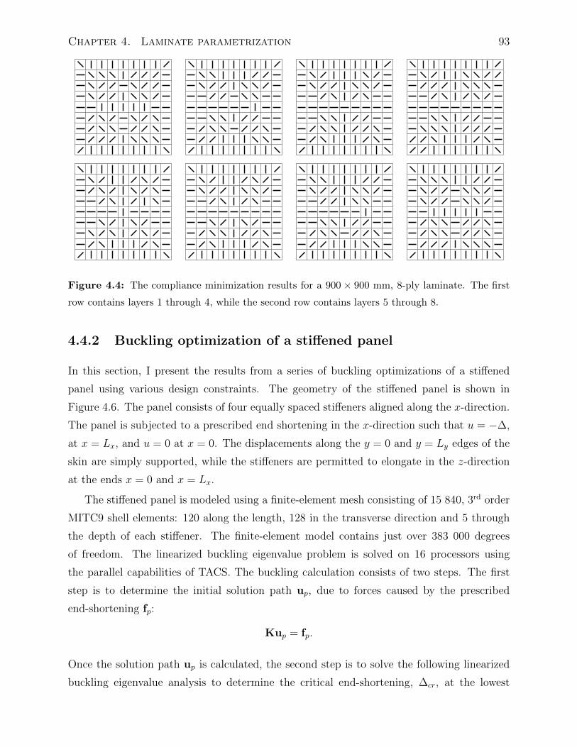
Chapter 4. Laminate parametrization 93
Figure 4.4: The compliance minimization results for a 900 × 900 mm, 8-ply laminate. The first
row contains layers 1 through 4, while the second row contains layers 5 through 8.
4.4.2 Buckling optimization of a stiffened panel
In this section, I present the results from a series of buckling optimizations of a stiffened
panel using various design constraints. The geometry of the stiffened panel is shown in
Figure 4.6. The panel consists of four equally spaced stiffeners aligned along the x-direction.
The panel is subjected to a prescribed end shortening in the x-direction such that u = −∆,
at x = Lx, and u = 0 at x = 0. The displacements along the y = 0 and y = Ly edges of the
skin are simply supported, while the stiffeners are permitted to elongate in the z-direction
at the ends x = 0 and x = Lx.
The stiffened panel is modeled using a finite-element mesh consisting of 15 840, 3rd order
MITC9 shell elements: 120 along the length, 128 in the transverse direction and 5 through
the depth of each stiffener. The finite-element model contains just over 383 000 degrees
of freedom. The linearized buckling eigenvalue problem is solved on 16 processors using
the parallel capabilities of TACS. The buckling calculation consists of two steps. The first
step is to determine the initial solution path up, due to forces caused by the prescribed
end-shortening fp:
Kup = fp.
Once the solution path up is calculated, the second step is to solve the following linearized
buckling eigenvalue analysis to determine the critical end-shortening, ∆cr, at the lowest
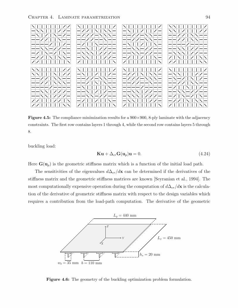
Chapter 4. Laminate parametrization 94
Figure 4.5: The compliance minimization results for a 900×900, 8-ply laminate with the adjacency
constraints. The first row contains layers 1 through 4, while the second row contains layers 5 through
8.
buckling load:
Ku + ∆crG(up)u = 0. (4.24)
Here G(up) is the geometric stiffness matrix which is a function of the initial load path.
The sensitivities of the eigenvalues d∆cr/dx can be determined if the derivatives of the
stiffness matrix and the geometric stiffness matrices are known [Seyranian et al., 1994]. The
most computationally expensive operation during the computation of d∆cr/dx is the calcula-
tion of the derivative of geometric stiffness matrix with respect to the design variables which
requires a contribution from the load-path computation. The derivative of the geometric
X
Y
Z
Ly = 440 mm
Lx = 450 mm
hs = 20 mm
b = 110 mmwb = 35 mm
Figure 4.6: The geometry of the buckling optimization problem formulation.
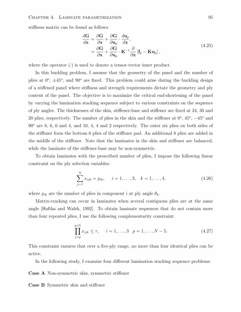
Chapter 4. Laminate parametrization 95
stiffness matrix can be found as follows:
dG
dx=∂G
∂x+∂G
∂up· dupdx
,
=∂G
∂x+∂G
∂up·K−1 ∂
∂x[fp −Kup] ,
(4.25)
where the operator (·) is used to denote a tensor-vector inner product.
In this buckling problem, I assume that the geometry of the panel and the number of
plies at 0o, ±45o, and 90o are fixed. This problem could arise during the buckling design
of a stiffened panel where stiffness and strength requirements dictate the geometry and ply
content of the panel. The objective is to maximize the critical end-shortening of the panel
by varying the lamination stacking sequence subject to various constraints on the sequence
of ply angles. The thicknesses of the skin, stiffener-base and stiffener are fixed at 24, 30 and
20 plies, respectively. The number of plies in the skin and the stiffener at 0o, 45o, −45o and
90o are 8, 6, 6 and 4, and 10, 4, 4 and 2 respectively. The outer six plies on both sides of
the stiffener form the bottom 6 plies of the stiffener pad. An additional 8 plies are added in
the middle of the stiffener. Note that the laminates in the skin and stiffener are balanced,
while the laminate of the stiffener-base may be non-symmetric.
To obtain laminates with the prescribed number of plies, I impose the following linear
constraint on the ply selection variables:
N∑j=1
xijk = pik, i = 1, . . . , 3, k = 1, . . . , 4, (4.26)
where pik are the number of plies in component i at ply angle θk.
Matrix-cracking can occur in laminates when several contiguous plies are at the same
angle [Haftka and Walsh, 1992]. To obtain laminate sequences that do not contain more
than four repeated plies, I use the following complementarity constraint:
p+5∏j=p
xijk ≤ τ, i = 1, . . . , 3 p = 1, . . . , N − 5. (4.27)
This constraint ensures that over a five-ply range, no more than four identical plies can be
active.
In the following study, I examine four different lamination stacking sequence problems:
Case A Non-symmetric skin, symmetric stiffener
Case B Symmetric skin and stiffener
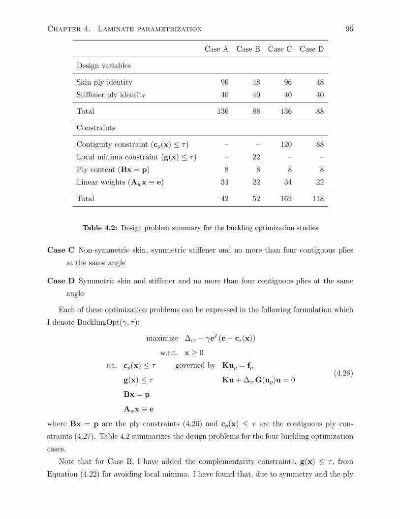
Chapter 4. Laminate parametrization 96
Case A Case B Case C Case D
Design variables
Skin ply identity 96 48 96 48
Stiffener ply identity 40 40 40 40
Total 136 88 136 88
Constraints
Contiguity constraint (cp(x) ≤ τ) – – 120 88
Local minima constraint (g(x) ≤ τ) – 22 – –
Ply content (Bx = p) 8 8 8 8
Linear weights (Awx ≡ e) 34 22 34 22
Total 42 52 162 118
Table 4.2: Design problem summary for the buckling optimization studies
Case C Non-symmetric skin, symmetric stiffener and no more than four contiguous plies
at the same angle
Case D Symmetric skin and stiffener and no more than four contiguous plies at the same
angle
Each of these optimization problems can be expressed in the following formulation which
I denote BucklingOpt(γ, τ):
maximize ∆cr − γeT (e− cs(x))
w.r.t. x ≥ 0
s.t. cp(x) ≤ τ governed by Kup = fp
g(x) ≤ τ Ku + ∆crG(up)u = 0
Bx = p
Awx ≡ e
(4.28)
where Bx = p are the ply constraints (4.26) and cp(x) ≤ τ are the contiguous ply con-
straints (4.27). Table 4.2 summarizes the design problems for the four buckling optimization
cases.
Note that for Case B, I have added the complementarity constraints, g(x) ≤ τ , from
Equation (4.22) for avoiding local minima. I have found that, due to symmetry and the ply
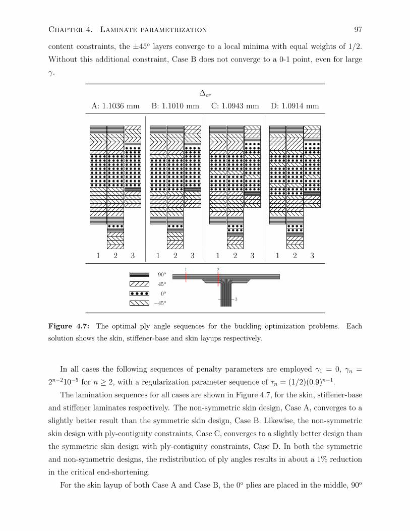
Chapter 4. Laminate parametrization 97
content constraints, the ±45o layers converge to a local minima with equal weights of 1/2.
Without this additional constraint, Case B does not converge to a 0-1 point, even for large
γ.
∆cr
A: 1.1036 mm B: 1.1010 mm C: 1.0943 mm D: 1.0914 mm
1 2 3 1 2 3 1 2 3 1 2 3
−45o0o
45o
90o1 2
3
Figure 4.7: The optimal ply angle sequences for the buckling optimization problems. Each
solution shows the skin, stiffener-base and skin layups respectively.
In all cases the following sequences of penalty parameters are employed γ1 = 0, γn =
2n−210−5 for n ≥ 2, with a regularization parameter sequence of τn = (1/2)(0.9)n−1.
The lamination sequences for all cases are shown in Figure 4.7, for the skin, stiffener-base
and stiffener laminates respectively. The non-symmetric skin design, Case A, converges to a
slightly better result than the symmetric skin design, Case B. Likewise, the non-symmetric
skin design with ply-contiguity constraints, Case C, converges to a slightly better design than
the symmetric skin design with ply-contiguity constraints, Case D. In both the symmetric
and non-symmetric designs, the redistribution of ply angles results in about a 1% reduction
in the critical end-shortening.
For the skin layup of both Case A and Case B, the 0o plies are placed in the middle, 90o
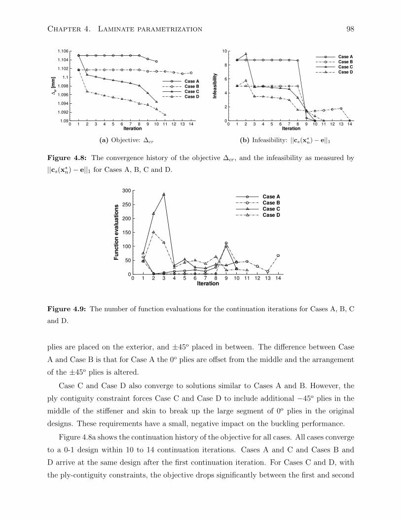
Chapter 4. Laminate parametrization 98
Iteration
∆cr[m
m]
0 1 2 3 4 5 6 7 8 9 10 11 12 13 141.09
1.092
1.094
1.096
1.098
1.1
1.102
1.104
1.106
Case A
Case B
Case C
Case D
(a) Objective: ∆cr
Iteration
Infeasibility
0 1 2 3 4 5 6 7 8 9 10 11 12 13 140
2
4
6
8
10
Case A
Case B
Case C
Case D
(b) Infeasibility: ||cs(x∗n)− e||1
Figure 4.8: The convergence history of the objective ∆cr, and the infeasibility as measured by
||cs(x∗n)− e||1 for Cases A, B, C and D.
Iteration
Functionevaluations
0 1 2 3 4 5 6 7 8 9 10 11 12 13 140
50
100
150
200
250
300
Case A
Case B
Case C
Case D
Figure 4.9: The number of function evaluations for the continuation iterations for Cases A, B, C
and D.
plies are placed on the exterior, and ±45o placed in between. The difference between Case
A and Case B is that for Case A the 0o plies are offset from the middle and the arrangement
of the ±45o plies is altered.
Case C and Case D also converge to solutions similar to Cases A and B. However, the
ply contiguity constraint forces Case C and Case D to include additional −45o plies in the
middle of the stiffener and skin to break up the large segment of 0o plies in the original
designs. These requirements have a small, negative impact on the buckling performance.
Figure 4.8a shows the continuation history of the objective for all cases. All cases converge
to a 0-1 design within 10 to 14 continuation iterations. Cases A and C and Cases B and
D arrive at the same design after the first continuation iteration. For Cases C and D, with
the ply-contiguity constraints, the objective drops significantly between the first and second
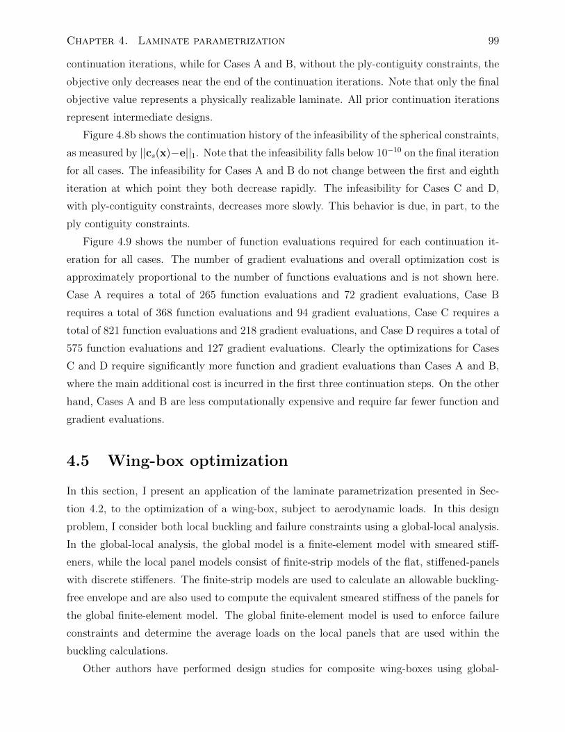
Chapter 4. Laminate parametrization 99
continuation iterations, while for Cases A and B, without the ply-contiguity constraints, the
objective only decreases near the end of the continuation iterations. Note that only the final
objective value represents a physically realizable laminate. All prior continuation iterations
represent intermediate designs.
Figure 4.8b shows the continuation history of the infeasibility of the spherical constraints,
as measured by ||cs(x)−e||1. Note that the infeasibility falls below 10−10 on the final iteration
for all cases. The infeasibility for Cases A and B do not change between the first and eighth
iteration at which point they both decrease rapidly. The infeasibility for Cases C and D,
with ply-contiguity constraints, decreases more slowly. This behavior is due, in part, to the
ply contiguity constraints.
Figure 4.9 shows the number of function evaluations required for each continuation it-
eration for all cases. The number of gradient evaluations and overall optimization cost is
approximately proportional to the number of functions evaluations and is not shown here.
Case A requires a total of 265 function evaluations and 72 gradient evaluations, Case B
requires a total of 368 function evaluations and 94 gradient evaluations, Case C requires a
total of 821 function evaluations and 218 gradient evaluations, and Case D requires a total of
575 function evaluations and 127 gradient evaluations. Clearly the optimizations for Cases
C and D require significantly more function and gradient evaluations than Cases A and B,
where the main additional cost is incurred in the first three continuation steps. On the other
hand, Cases A and B are less computationally expensive and require far fewer function and
gradient evaluations.
4.5 Wing-box optimization
In this section, I present an application of the laminate parametrization presented in Sec-
tion 4.2, to the optimization of a wing-box, subject to aerodynamic loads. In this design
problem, I consider both local buckling and failure constraints using a global-local analysis.
In the global-local analysis, the global model is a finite-element model with smeared stiff-
eners, while the local panel models consist of finite-strip models of the flat, stiffened-panels
with discrete stiffeners. The finite-strip models are used to calculate an allowable buckling-
free envelope and are also used to compute the equivalent smeared stiffness of the panels for
the global finite-element model. The global finite-element model is used to enforce failure
constraints and determine the average loads on the local panels that are used within the
buckling calculations.
Other authors have performed design studies for composite wing-boxes using global-
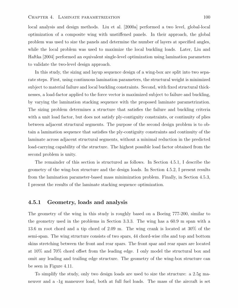
Chapter 4. Laminate parametrization 100
local analysis and design methods. Liu et al. [2000a] performed a two level, global-local
optimization of a composite wing with unstiffened panels. In their approach, the global
problem was used to size the panels and determine the number of layers at specified angles,
while the local problem was used to maximize the local buckling loads. Later, Liu and
Haftka [2004] performed an equivalent single-level optimization using lamination parameters
to validate the two-level design approach.
In this study, the sizing and layup sequence design of a wing-box are split into two sepa-
rate steps. First, using continuous lamination parameters, the structural weight is minimized
subject to material failure and local buckling constraints. Second, with fixed structural thick-
nesses, a load-factor applied to the force vector is maximized subject to failure and buckling,
by varying the lamination stacking sequence with the proposed laminate parametrization.
The sizing problem determines a structure that satisfies the failure and buckling criteria
with a unit load factor, but does not satisfy ply-contiguity constraints, or continuity of plies
between adjacent structural segments. The purpose of the second design problem is to ob-
tain a lamination sequence that satisfies the ply-contiguity constraints and continuity of the
laminate across adjacent structural segments, without a minimal reduction in the predicted
load-carrying capability of the structure. The highest possible load factor obtained from the
second problem is unity.
The remainder of this section is structured as follows. In Section 4.5.1, I describe the
geometry of the wing-box structure and the design loads. In Section 4.5.2, I present results
from the lamination parameter-based mass minimization problem. Finally, in Section 4.5.3,
I present the results of the laminate stacking sequence optimization.
4.5.1 Geometry, loads and analysis
The geometry of the wing in this study is roughly based on a Boeing 777-200, similar to
the geometry used in the problems in Section 3.3.3. The wing has a 60.9 m span with a
13.6 m root chord and a tip chord of 2.09 m. The wing crank is located at 30% of the
semi-span. The wing structure consists of two spars, 44 chord-wise ribs and top and bottom
skins stretching between the front and rear spars. The front spar and rear spars are located
at 10% and 70% chord offset from the leading edge. I only model the structural box and
omit any leading and trailing edge structure. The geometry of the wing-box structure can
be seen in Figure 4.11.
To simplify the study, only two design loads are used to size the structure: a 2.5g ma-
neuver and a -1g maneuver load, both at full fuel loads. The mass of the aircraft is set
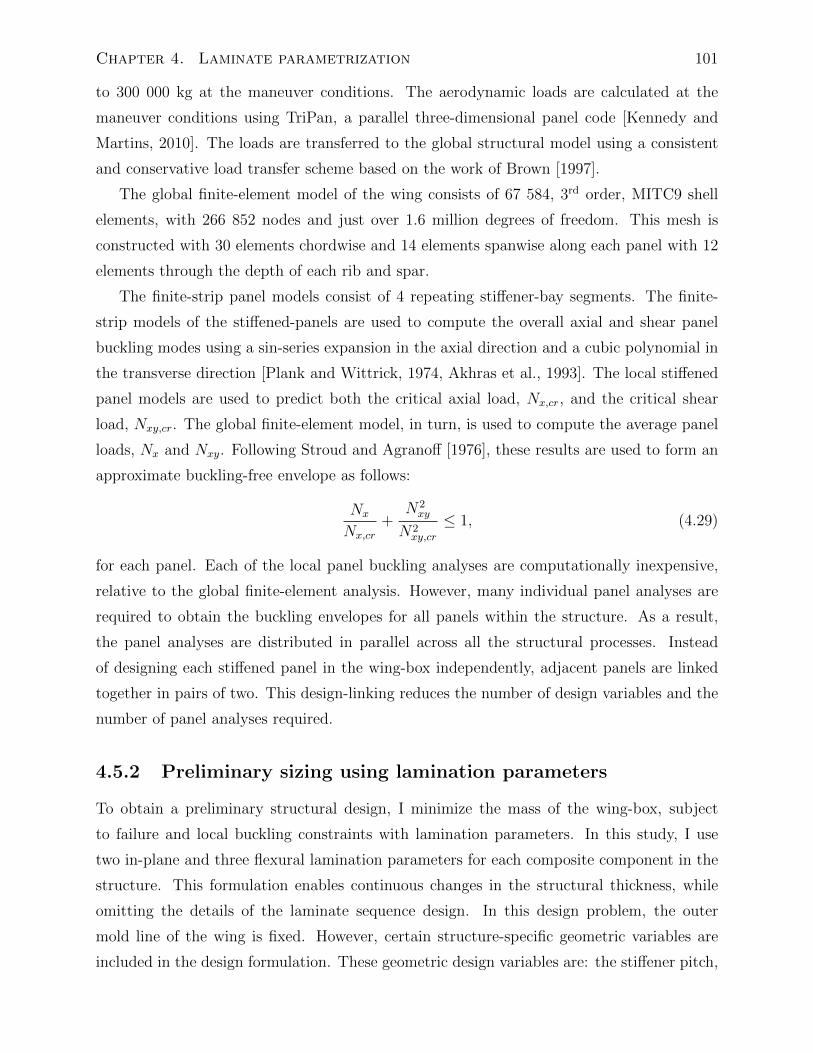
Chapter 4. Laminate parametrization 101
to 300 000 kg at the maneuver conditions. The aerodynamic loads are calculated at the
maneuver conditions using TriPan, a parallel three-dimensional panel code [Kennedy and
Martins, 2010]. The loads are transferred to the global structural model using a consistent
and conservative load transfer scheme based on the work of Brown [1997].
The global finite-element model of the wing consists of 67 584, 3rd order, MITC9 shell
elements, with 266 852 nodes and just over 1.6 million degrees of freedom. This mesh is
constructed with 30 elements chordwise and 14 elements spanwise along each panel with 12
elements through the depth of each rib and spar.
The finite-strip panel models consist of 4 repeating stiffener-bay segments. The finite-
strip models of the stiffened-panels are used to compute the overall axial and shear panel
buckling modes using a sin-series expansion in the axial direction and a cubic polynomial in
the transverse direction [Plank and Wittrick, 1974, Akhras et al., 1993]. The local stiffened
panel models are used to predict both the critical axial load, Nx,cr, and the critical shear
load, Nxy,cr. The global finite-element model, in turn, is used to compute the average panel
loads, Nx and Nxy. Following Stroud and Agranoff [1976], these results are used to form an
approximate buckling-free envelope as follows:
Nx
Nx,cr
+N2xy
N2xy,cr
≤ 1, (4.29)
for each panel. Each of the local panel buckling analyses are computationally inexpensive,
relative to the global finite-element analysis. However, many individual panel analyses are
required to obtain the buckling envelopes for all panels within the structure. As a result,
the panel analyses are distributed in parallel across all the structural processes. Instead
of designing each stiffened panel in the wing-box independently, adjacent panels are linked
together in pairs of two. This design-linking reduces the number of design variables and the
number of panel analyses required.
4.5.2 Preliminary sizing using lamination parameters
To obtain a preliminary structural design, I minimize the mass of the wing-box, subject
to failure and local buckling constraints with lamination parameters. In this study, I use
two in-plane and three flexural lamination parameters for each composite component in the
structure. This formulation enables continuous changes in the structural thickness, while
omitting the details of the laminate sequence design. In this design problem, the outer
mold line of the wing is fixed. However, certain structure-specific geometric variables are
included in the design formulation. These geometric design variables are: the stiffener pitch,
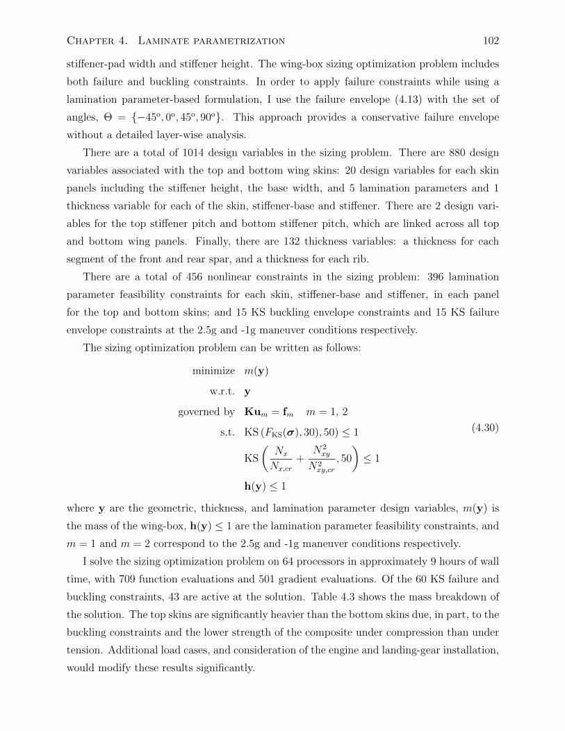
Chapter 4. Laminate parametrization 102
stiffener-pad width and stiffener height. The wing-box sizing optimization problem includes
both failure and buckling constraints. In order to apply failure constraints while using a
lamination parameter-based formulation, I use the failure envelope (4.13) with the set of
angles, Θ = −45o, 0o, 45o, 90o. This approach provides a conservative failure envelope
without a detailed layer-wise analysis.
There are a total of 1014 design variables in the sizing problem. There are 880 design
variables associated with the top and bottom wing skins: 20 design variables for each skin
panels including the stiffener height, the base width, and 5 lamination parameters and 1
thickness variable for each of the skin, stiffener-base and stiffener. There are 2 design vari-
ables for the top stiffener pitch and bottom stiffener pitch, which are linked across all top
and bottom wing panels. Finally, there are 132 thickness variables: a thickness for each
segment of the front and rear spar, and a thickness for each rib.
There are a total of 456 nonlinear constraints in the sizing problem: 396 lamination
parameter feasibility constraints for each skin, stiffener-base and stiffener, in each panel
for the top and bottom skins; and 15 KS buckling envelope constraints and 15 KS failure
envelope constraints at the 2.5g and -1g maneuver conditions respectively.
The sizing optimization problem can be written as follows:
minimize m(y)
w.r.t. y
governed by Kum = fm m = 1, 2
s.t. KS (FKS(σ), 30), 50) ≤ 1
KS
(Nx
Nx,cr
+N2xy
N2xy,cr
, 50
)≤ 1
h(y) ≤ 1
(4.30)
where y are the geometric, thickness, and lamination parameter design variables, m(y) is
the mass of the wing-box, h(y) ≤ 1 are the lamination parameter feasibility constraints, and
m = 1 and m = 2 correspond to the 2.5g and -1g maneuver conditions respectively.
I solve the sizing optimization problem on 64 processors in approximately 9 hours of wall
time, with 709 function evaluations and 501 gradient evaluations. Of the 60 KS failure and
buckling constraints, 43 are active at the solution. Table 4.3 shows the mass breakdown of
the solution. The top skins are significantly heavier than the bottom skins due, in part, to the
buckling constraints and the lower strength of the composite under compression than under
tension. Additional load cases, and consideration of the engine and landing-gear installation,
would modify these results significantly.
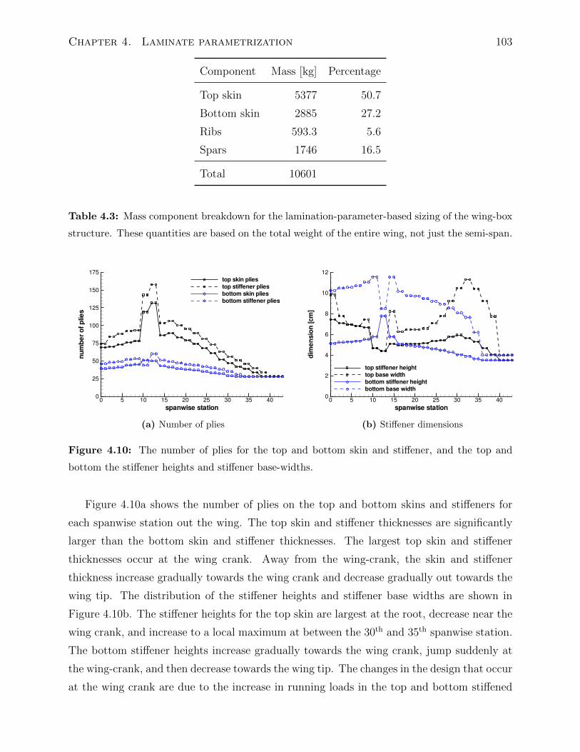
Chapter 4. Laminate parametrization 103
Component Mass [kg] Percentage
Top skin 5377 50.7
Bottom skin 2885 27.2
Ribs 593.3 5.6
Spars 1746 16.5
Total 10601
Table 4.3: Mass component breakdown for the lamination-parameter-based sizing of the wing-box
structure. These quantities are based on the total weight of the entire wing, not just the semi-span.
spanwise station
numberofplies
0 5 10 15 20 25 30 35 400
25
50
75
100
125
150
175
top skin plies
top stiffener plies
bottom skin plies
bottom stiffener plies
(a) Number of plies
spanwise station
dim
ension[cm]
0 5 10 15 20 25 30 35 400
2
4
6
8
10
12
top stiffener height
top base width
bottom stiffener height
bottom base width
(b) Stiffener dimensions
Figure 4.10: The number of plies for the top and bottom skin and stiffener, and the top and
bottom the stiffener heights and stiffener base-widths.
Figure 4.10a shows the number of plies on the top and bottom skins and stiffeners for
each spanwise station out the wing. The top skin and stiffener thicknesses are significantly
larger than the bottom skin and stiffener thicknesses. The largest top skin and stiffener
thicknesses occur at the wing crank. Away from the wing-crank, the skin and stiffener
thickness increase gradually towards the wing crank and decrease gradually out towards the
wing tip. The distribution of the stiffener heights and stiffener base widths are shown in
Figure 4.10b. The stiffener heights for the top skin are largest at the root, decrease near the
wing crank, and increase to a local maximum at between the 30th and 35th spanwise station.
The bottom stiffener heights increase gradually towards the wing crank, jump suddenly at
the wing-crank, and then decrease towards the wing tip. The changes in the design that occur
at the wing crank are due to the increase in running loads in the top and bottom stiffened
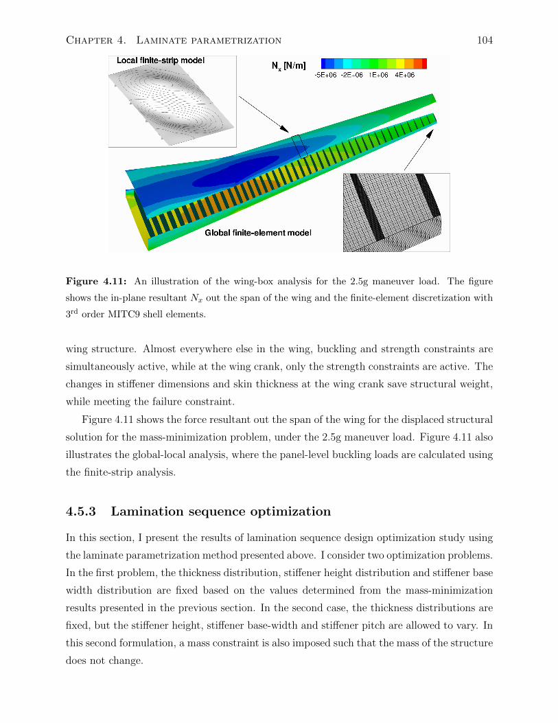
Chapter 4. Laminate parametrization 104
Figure 4.11: An illustration of the wing-box analysis for the 2.5g maneuver load. The figure
shows the in-plane resultant Nx out the span of the wing and the finite-element discretization with
3rd order MITC9 shell elements.
wing structure. Almost everywhere else in the wing, buckling and strength constraints are
simultaneously active, while at the wing crank, only the strength constraints are active. The
changes in stiffener dimensions and skin thickness at the wing crank save structural weight,
while meeting the failure constraint.
Figure 4.11 shows the force resultant out the span of the wing for the displaced structural
solution for the mass-minimization problem, under the 2.5g maneuver load. Figure 4.11 also
illustrates the global-local analysis, where the panel-level buckling loads are calculated using
the finite-strip analysis.
4.5.3 Lamination sequence optimization
In this section, I present the results of lamination sequence design optimization study using
the laminate parametrization method presented above. I consider two optimization problems.
In the first problem, the thickness distribution, stiffener height distribution and stiffener base
width distribution are fixed based on the values determined from the mass-minimization
results presented in the previous section. In the second case, the thickness distributions are
fixed, but the stiffener height, stiffener base-width and stiffener pitch are allowed to vary. In
this second formulation, a mass constraint is also imposed such that the mass of the structure
does not change.
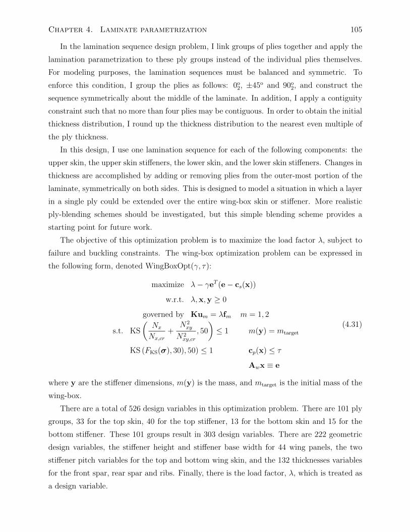
Chapter 4. Laminate parametrization 105
In the lamination sequence design problem, I link groups of plies together and apply the
lamination parametrization to these ply groups instead of the individual plies themselves.
For modeling purposes, the lamination sequences must be balanced and symmetric. To
enforce this condition, I group the plies as follows: 0o2, ±45o and 90o
2, and construct the
sequence symmetrically about the middle of the laminate. In addition, I apply a contiguity
constraint such that no more than four plies may be contiguous. In order to obtain the initial
thickness distribution, I round up the thickness distribution to the nearest even multiple of
the ply thickness.
In this design, I use one lamination sequence for each of the following components: the
upper skin, the upper skin stiffeners, the lower skin, and the lower skin stiffeners. Changes in
thickness are accomplished by adding or removing plies from the outer-most portion of the
laminate, symmetrically on both sides. This is designed to model a situation in which a layer
in a single ply could be extended over the entire wing-box skin or stiffener. More realistic
ply-blending schemes should be investigated, but this simple blending scheme provides a
starting point for future work.
The objective of this optimization problem is to maximize the load factor λ, subject to
failure and buckling constraints. The wing-box optimization problem can be expressed in
the following form, denoted WingBoxOpt(γ, τ):
maximize λ− γeT (e− cs(x))
w.r.t. λ,x,y ≥ 0
governed by Kum = λfm m = 1, 2
s.t. KS
(Nx
Nx,cr
+N2xy
N2xy,cr
, 50
)≤ 1 m(y) = mtarget
KS (FKS(σ), 30), 50) ≤ 1 cp(x) ≤ τ
Awx ≡ e
(4.31)
where y are the stiffener dimensions, m(y) is the mass, and mtarget is the initial mass of the
wing-box.
There are a total of 526 design variables in this optimization problem. There are 101 ply
groups, 33 for the top skin, 40 for the top stiffener, 13 for the bottom skin and 15 for the
bottom stiffener. These 101 groups result in 303 design variables. There are 222 geometric
design variables, the stiffener height and stiffener base width for 44 wing panels, the two
stiffener pitch variables for the top and bottom wing skin, and the 132 thicknesses variables
for the front spar, rear spar and ribs. Finally, there is the load factor, λ, which is treated as
a design variable.
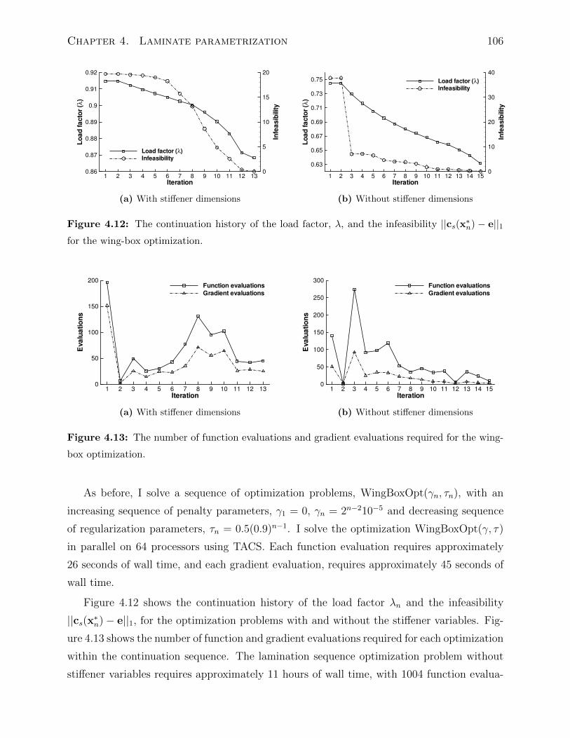
Chapter 4. Laminate parametrization 106
Iteration
Loadfactor(λ)
Infeasibility
1 2 3 4 5 6 7 8 9 10 11 12 130.86
0.87
0.88
0.89
0.9
0.91
0.92
0
5
10
15
20
Load factor (λ)
Infeasibility
(a) With stiffener dimensions
Iteration
Loadfactor(λ)
Infeasibility
1 2 3 4 5 6 7 8 9 10 11 12 13 14 15
0.63
0.65
0.67
0.69
0.71
0.73
0.75
0
10
20
30
40
Load factor (λ)
Infeasibility
(b) Without stiffener dimensions
Figure 4.12: The continuation history of the load factor, λ, and the infeasibility ||cs(x∗n) − e||1for the wing-box optimization.
Iteration
Evaluations
1 2 3 4 5 6 7 8 9 10 11 12 130
50
100
150
200Function evaluations
Gradient evaluations
(a) With stiffener dimensions
Iteration
Evaluations
1 2 3 4 5 6 7 8 9 10 11 12 13 14 150
50
100
150
200
250
300Function evaluations
Gradient evaluations
(b) Without stiffener dimensions
Figure 4.13: The number of function evaluations and gradient evaluations required for the wing-
box optimization.
As before, I solve a sequence of optimization problems, WingBoxOpt(γn, τn), with an
increasing sequence of penalty parameters, γ1 = 0, γn = 2n−210−5 and decreasing sequence
of regularization parameters, τn = 0.5(0.9)n−1. I solve the optimization WingBoxOpt(γ, τ)
in parallel on 64 processors using TACS. Each function evaluation requires approximately
26 seconds of wall time, and each gradient evaluation, requires approximately 45 seconds of
wall time.
Figure 4.12 shows the continuation history of the load factor λn and the infeasibility
||cs(x∗n)− e||1, for the optimization problems with and without the stiffener variables. Fig-
ure 4.13 shows the number of function and gradient evaluations required for each optimization
within the continuation sequence. The lamination sequence optimization problem without
stiffener variables requires approximately 11 hours of wall time, with 1004 function evalua-
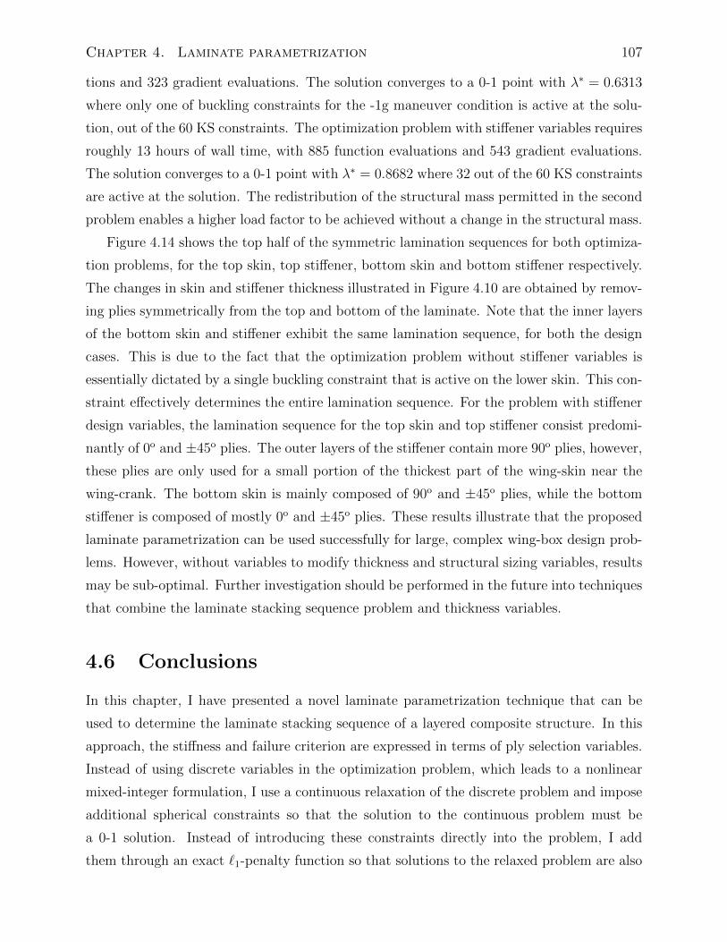
Chapter 4. Laminate parametrization 107
tions and 323 gradient evaluations. The solution converges to a 0-1 point with λ∗ = 0.6313
where only one of buckling constraints for the -1g maneuver condition is active at the solu-
tion, out of the 60 KS constraints. The optimization problem with stiffener variables requires
roughly 13 hours of wall time, with 885 function evaluations and 543 gradient evaluations.
The solution converges to a 0-1 point with λ∗ = 0.8682 where 32 out of the 60 KS constraints
are active at the solution. The redistribution of the structural mass permitted in the second
problem enables a higher load factor to be achieved without a change in the structural mass.
Figure 4.14 shows the top half of the symmetric lamination sequences for both optimiza-
tion problems, for the top skin, top stiffener, bottom skin and bottom stiffener respectively.
The changes in skin and stiffener thickness illustrated in Figure 4.10 are obtained by remov-
ing plies symmetrically from the top and bottom of the laminate. Note that the inner layers
of the bottom skin and stiffener exhibit the same lamination sequence, for both the design
cases. This is due to the fact that the optimization problem without stiffener variables is
essentially dictated by a single buckling constraint that is active on the lower skin. This con-
straint effectively determines the entire lamination sequence. For the problem with stiffener
design variables, the lamination sequence for the top skin and top stiffener consist predomi-
nantly of 0o and ±45o plies. The outer layers of the stiffener contain more 90o plies, however,
these plies are only used for a small portion of the thickest part of the wing-skin near the
wing-crank. The bottom skin is mainly composed of 90o and ±45o plies, while the bottom
stiffener is composed of mostly 0o and ±45o plies. These results illustrate that the proposed
laminate parametrization can be used successfully for large, complex wing-box design prob-
lems. However, without variables to modify thickness and structural sizing variables, results
may be sub-optimal. Further investigation should be performed in the future into techniques
that combine the laminate stacking sequence problem and thickness variables.
4.6 Conclusions
In this chapter, I have presented a novel laminate parametrization technique that can be
used to determine the laminate stacking sequence of a layered composite structure. In this
approach, the stiffness and failure criterion are expressed in terms of ply selection variables.
Instead of using discrete variables in the optimization problem, which leads to a nonlinear
mixed-integer formulation, I use a continuous relaxation of the discrete problem and impose
additional spherical constraints so that the solution to the continuous problem must be
a 0-1 solution. Instead of introducing these constraints directly into the problem, I add
them through an exact `1-penalty function so that solutions to the relaxed problem are also
Chapter 4. Laminate parametrization 108
solutions to the penalized problem, for sufficiently large values of the penalty parameter
γ. Additional simplifications can be achieved if the set of linear constraints on the ply-
identity variables are satisfied exactly at every iteration in the optimization problem. This
approach can be used as an independent penalization, or as an additional penalization to
discrete material optimization (DMO) parametrizations that use a SIMP-approach. I applied
the proposed parametrization technique to a series of structural optimization problems of
increasing complexity, including a wing-box lamination sequence optimization. These results
demonstrate that the proposed parametrization method is an effective approach to obtain
0-1 designs for large, complex lamination sequence design problems.
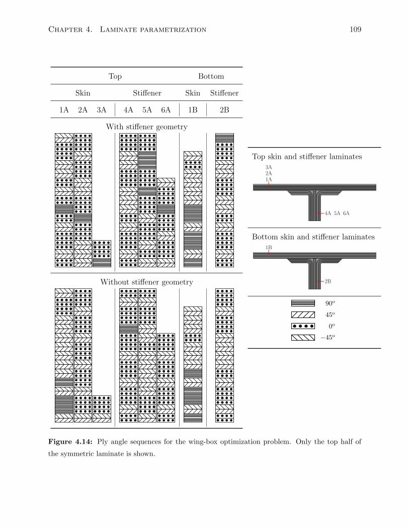
Chapter 4. Laminate parametrization 109
Top Bottom
Skin Stiffener Skin Stiffener
1A 2A 3A 4A 5A 6A 1B 2B
With stiffener geometry
Without stiffener geometry
Top skin and stiffener laminates
1A2A3A
4A 5A 6A
Bottom skin and stiffener laminates1B
2B
−45o0o
45o
90o
Figure 4.14: Ply angle sequences for the wing-box optimization problem. Only the top half of
the symmetric laminate is shown.

Chapter 5
Aerostructural analysis and design
optimization
Aerostructural design optimization using high-fidelity models is a computationally intensive
multidisciplinary design optimization problem. Many authors have focused on using high-
fidelity aerodynamic analysis in the aerostructural problem, while using considerably smaller
finite-element models. This discrepancy is often justified since the primary area of interest in
these studies is the aerodynamic performance of the aerostructural system. Several authors
have devised optimization techniques specifically designed to take advantage of this imbal-
ance [Chittick and Martins, 2008, 2009, Kennedy et al., 2008]. However, it is also important
to examine the consequences of larger and more sophisticated structural analyses, and the
implications these more costly structural models have on both aerostructural solution algo-
rithms and the aerostructural optimization problem. Examining these consequences is an
important research problem, as unconventional aircraft design concepts and the increasing
use of composites and advanced composite systems place additional computational demands
on both the structural and aerodynamic analyses.
In this chapter, I present an aerostructural analysis and design optimization framework
that is designed to be efficient when both the aerodynamic and structural disciplines require
significant computational resources and time. This situation leads to aerostructural solution
and sensitivity methods that separate the computational resources of the disciplines. In the
present work, the aerodynamic analysis uses a parallel, three-dimensional panel code, Tri-
Pan, coupled to the finite-element code TACS, described in greater detail in Chapter 3. The
inter-disciplinary coupling is handled using a parallel implementation of a consistent and
conservative load and displacement transfer technique. While TriPan is a medium fidelity
aerodynamic analysis tool, it does provide accurate induced drag, lift, and pressure distri-
110
Chapter 5. Aerostructural analysis and design optimization 111
bution results at low to moderate Mach numbers. Furthermore, TriPan requires significant
computational time and resources for large aerodynamic meshes. The framework presented
here has been successfully extended and integrated with a high-fidelity aerodynamic anal-
ysis tool, the Stanford University multi-block (SUmb) solver [Kenway et al., 2012]. The
work presented here should be regarded as a first step towards fully integrated high-fidelity
multidisciplinary analysis and optimization, with special attention paid to the structural
problem.
The remainder of this chapter is organized as follows: In Section 5.1, I present a re-
view of significant contributions to the literature in the areas of aerostructural analysis and
design optimization. In Section 5.2, I outline the components of the present aerostruc-
tural design optimization framework, including the aerodynamic analysis performed using
the three-dimensional panel code TriPan, the structural analysis performed using TACS,
the load and displacement transfer approach, and the geometric parametrization technique.
In Section 5.3, I describe the aerostructural solution methods that are used to solve the
coupled aerostructural system. In Section 5.4, I present the coupled aerostructural adjoint
sensitivity method. Finally, I present results for various aerostructural optimization studies
in Section 5.5.
5.1 Review of aerostructural optimization
Many authors have developed methods for aerostructural analysis and design optimization.
Reuther et al. [1999] developed an aerostructural analysis and optimization framework that
coupled a linear finite-element structural model to a finite-volume Euler CFD solver. They
obtained a coupled solution to the aerostructural system using a pseudo-time marching
scheme with periodic updates of the displaced shape. Their structural model consisted of
either solid, three-dimensional elements, to represent a wind tunnel wing model, or shell and
beam elements to represent a stiffened aircraft wing. Following the work of Brown [1997],
they developed a systematic scheme to pass loads and displacements across the aircraft outer
mould line (OML). Martins et al. [2005] developed both an adjoint and direct sensitivity
formulation for the coupled aerostructural system, and implemented a solution method for
the coupled adjoint system based on a block Gauss–Seidel technique. Martins et al. [2004]
applied this framework to the optimization of a supersonic business jet.
Maute et al. [2001] performed an aerostructural analysis that coupled the an Euler CFD
solver to a linear finite-element structural model. They employed a mesh movement strategy
based on a spring analogy and a load and displacement transfer technique following the
Chapter 5. Aerostructural analysis and design optimization 112
earlier work of Maman and Farhat [1995] and Farhat et al. [1996]. Maute et al. used a
nonlinear block Gauss–Seidel method with relaxation for the solution of the coupled nonlinear
equations. Furthermore, they presented formulations of both the adjoint and direct methods
for computing the sensitivities of the coupled aerostructural system. These linear equations
were solved using a block Gauss–Seidel method that mirrors the method of solution for the
coupled system. Two types of structural models were employed: an equivalent flat plate
composed of either a single isotropic material or multiple composite layers and a full shell
and stiffener model composed of shell and beam elements.
Later, Maute and Allen [2004], using a similar aerostructural solution and sensitivity
techniques as Maute et al. [2001], developed an aerostructural optimization problem in which
the internal structure of the wing box was parametrized using a single isotropic material with
penalization (SIMP) approach. Maute and Allen used the SIMP method to determine the
topology of the optimal structure.
In order to improve the robustness and efficiency of the methods developed by Maute
et al. [2001], Barcelos et al. [2006] developed a class of Newton–Krylov–Schur methods for
solving the coupled nonlinear fluid-structure-mesh movement problem. In their approach,
a globalized Newton’s method is used to solve the coupled system. At each iteration, the
linearized system is solved using a Schur complement approach. They found that their
technique is more robust and efficient than the original Gauss–Seidel method presented by
Maute et al. [2001]. More recently, Barcelos and Maute [2008] presented an aerostructural
solution technique coupling a Navier–Stokes solver, including a turbulence model, to a lin-
ear finite-element structural analysis and a mesh movement strategy using a linear spring
analogy.
Aerostructural analysis techniques are a specialization of more general fluid-structure
interaction solution methods. A significant amount of research has focused on this field.
For instance, Felippa et al. [2001] performed an extensive review of solution techniques for
coupled nonlinear problems using partitioned solvers. Kim et al. [2003] developed a solution
procedure for coupled multi-physics problems using a multi-level Newton’s method. They
applied their approach to a coupled fluid-structure interaction problem, noting the impor-
tance of using an accurate linearization of the coupling terms. In two papers, Biros and
Ghattas [2005a,b] presented a Lagrange–Newton–Krylov–Schur approach to the simultane-
ous solution of PDE-constrained optimization problems. They applied their approach to a
design problem using the incompressible Navier–Stokes equations. Heil et al. [2008] solved
a time-dependent fluid-structure interaction problem by applying Newton’s method to a
second-order backward difference discretization of the coupled system. The resulting equa-
Chapter 5. Aerostructural analysis and design optimization 113
tions were solved using a fully-coupled approach, without neglecting coupling terms in the
linearization, with both direct and iterative solvers. They demonstrated that fully-coupled
methods are competitive with loosely-coupled methods that do not use coupling terms in
the linearization, even in cases of relatively weak coupling.
5.1.1 Load and displacement transfer schemes
One of the primary tasks in aerostructural analysis is to develop a scheme to couple the
aerodynamic and structural disciplines into a single analysis. Many authors have devised load
and displacement transfer techniques and a brief overview of some important contributions
is covered below.
Maman and Farhat [1995] developed a method for the direct transfer of loads and displace-
ments between fluid and structural meshes where the boundaries of the two domains may
not be coincident everywhere. In their scheme, pressure from the fluid mesh is transferred
to a projected point on the structural mesh, where a local normal is defined. For displace-
ment transfer, structural displacements are projected back onto the fluid mesh. From the
projected points, local interpolations are used to determine the values of the quantities of
interest. In a second paper, Farhat et al. [1996] devised two methods for load and displace-
ment transfer for transient problems: a method based on consistent interpolation between
coincident surfaces, and a second, more general method based on displacement and load
transfer between discrete surfaces.
Brown [1997] focused on the development of load and displacement transfer schemes
where the structural and fluid model are non-conforming. Brown used displacement interpo-
lation functions that are either a continuous extension of the finite-element shape functions,
or a rigid attachment to the nodal degrees of freedom. Brown constructed the load transfer
from the fluid to structural model using the principle of virtual work. This technique is
consistent (i.e. the sum of the forces on the fluid model is equal to the sum of the nodal
forces on the structure), and is also conservative (i.e. the work done on the fluid model in
moving through the displacements defined by the structure, is equal to the work performed
on the structure).
In two recent papers, Allen and Rendall [2007] and Rendall and Allen [2008] developed
interpolation and mesh movement schemes that employ radial basis functions (RBFs). In
these methods, the structural and aerodynamic models are embedded in an RBF volume.
Structural displacements are transferred through the volume using RBF displacement in-
terpolation. Load transfer is performed using the principle of virtual work. Consistency is
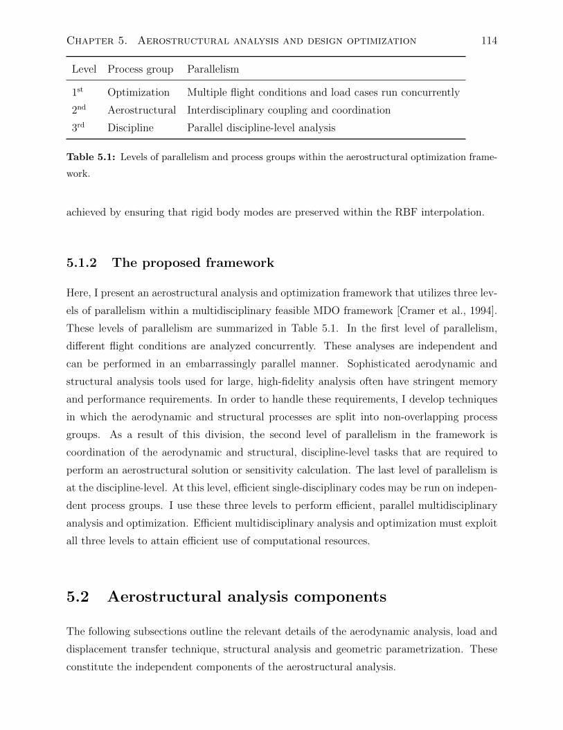
Chapter 5. Aerostructural analysis and design optimization 114
Level Process group Parallelism
1st Optimization Multiple flight conditions and load cases run concurrently
2nd Aerostructural Interdisciplinary coupling and coordination
3rd Discipline Parallel discipline-level analysis
Table 5.1: Levels of parallelism and process groups within the aerostructural optimization frame-
work.
achieved by ensuring that rigid body modes are preserved within the RBF interpolation.
5.1.2 The proposed framework
Here, I present an aerostructural analysis and optimization framework that utilizes three lev-
els of parallelism within a multidisciplinary feasible MDO framework [Cramer et al., 1994].
These levels of parallelism are summarized in Table 5.1. In the first level of parallelism,
different flight conditions are analyzed concurrently. These analyses are independent and
can be performed in an embarrassingly parallel manner. Sophisticated aerodynamic and
structural analysis tools used for large, high-fidelity analysis often have stringent memory
and performance requirements. In order to handle these requirements, I develop techniques
in which the aerodynamic and structural processes are split into non-overlapping process
groups. As a result of this division, the second level of parallelism in the framework is
coordination of the aerodynamic and structural, discipline-level tasks that are required to
perform an aerostructural solution or sensitivity calculation. The last level of parallelism is
at the discipline-level. At this level, efficient single-disciplinary codes may be run on indepen-
dent process groups. I use these three levels to perform efficient, parallel multidisciplinary
analysis and optimization. Efficient multidisciplinary analysis and optimization must exploit
all three levels to attain efficient use of computational resources.
5.2 Aerostructural analysis components
The following subsections outline the relevant details of the aerodynamic analysis, load and
displacement transfer technique, structural analysis and geometric parametrization. These
constitute the independent components of the aerostructural analysis.
Chapter 5. Aerostructural analysis and design optimization 115
5.2.1 TriPan: An aerodynamic panel code
Within the present aerostructural framework, the aerodynamic analysis is performed using
TriPan, an unstructured three-dimensional panel code for calculating the aerodynamic char-
acteristics of inviscid, external lifting flows governed by the Prandtl–Glauert equation [Katz
and Plotkin, 1991]. TriPan uses constant source and doublet singularity elements distributed
over the surface of a body discretized with quadrilateral and triangular panels [Katz and
Plotkin, 1991, Hess and Smith, 1967]. Aerodynamic forces and moments are calculated
using surface pressure integration. The induced drag is calculated using a far-field wake
integration scheme that provides a more accurate drag estimate than surface pressure in-
tegration [Smith, 1996]. The discretized set of boundary conditions governing the doublet
strengths are represented by the vector of aerodynamic residuals,
RA(w,u) = 0, (5.1)
where w is a vector of doublet strengths and u is a vector of the structural displacements.
I solve the linear system represented by Equation (5.1) using the parallel linear algebra
routines in PETSc [Balay et al., 2004, 1997]. A dense matrix storage format is used to
store the aerodynamic influence coefficients for each panel. The matrix is split between
processors such that the rows of the matrix are stored in contiguous segments on different
processors. The ownership range of each segment is determined by performing a domain
decomposition of the surface mesh using METIS [Karypis and Kumar, 1998] to determine
the surface-panel processor assignment. For efficiency reasons, each processor has a local
copy of the entire mesh. The surface mesh is relatively small, so copying the entire mesh
is not too costly in terms of memory when compared to the dense aerodynamic influence
coefficient matrix. I have also implemented an adjoint sensitivity method within TriPan that
may be used to compute the sensitivities of common functions of interest for gradient-based
design optimization.
I solve the linear system of equations represented by Equation (5.1) or the correspond-
ing adjoint system using GMRES(30) [Saad and Schultz, 1986] with a block-Jacobi ILU(0)
preconditioner. The preconditioner is assembled by considering only those panels that are
within a predetermined physical radius of the current panel centroid. The rationale for this
construction is that the closest panels have the strongest effect on a given panel. The effect
of a higher ILU preconditioner level of fill can be achieved by selecting a larger radius.
Figure 5.1 shows the timing results for both an aerodynamic analysis and sensitivity
evaluation for a TriPan model of a straight wing with aspect ratio 10, composed of NACA0012
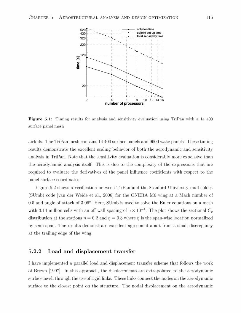
Chapter 5. Aerostructural analysis and design optimization 116
number of processors
time[s]
2 4 6 8 10 12 14 16
20
120
220
320
420
520 solution time
adjoint set up time
total sensitivity time
Figure 5.1: Timing results for analysis and sensitivity evaluation using TriPan with a 14 400
surface panel mesh
airfoils. The TriPan mesh contains 14 400 surface panels and 9600 wake panels. These timing
results demonstrate the excellent scaling behavior of both the aerodynamic and sensitivity
analysis in TriPan. Note that the sensitivity evaluation is considerably more expensive than
the aerodynamic analysis itself. This is due to the complexity of the expressions that are
required to evaluate the derivatives of the panel influence coefficients with respect to the
panel surface coordinates.
Figure 5.2 shows a verification between TriPan and the Stanford University multi-block
(SUmb) code [van der Weide et al., 2006] for the ONERA M6 wing at a Mach number of
0.5 and angle of attack of 3.06o. Here, SUmb is used to solve the Euler equations on a mesh
with 3.14 million cells with an off wall spacing of 5× 10⁻⁴. The plot shows the sectional Cp
distribution at the stations η = 0.2 and η = 0.8 where η is the span-wise location normalized
by semi-span. The results demonstrate excellent agreement apart from a small discrepancy
at the trailing edge of the wing.
5.2.2 Load and displacement transfer
I have implemented a parallel load and displacement transfer scheme that follows the work
of Brown [1997]. In this approach, the displacements are extrapolated to the aerodynamic
surface mesh through the use of rigid links. These links connect the nodes on the aerodynamic
surface to the closest point on the structure. The nodal displacement on the aerodynamic
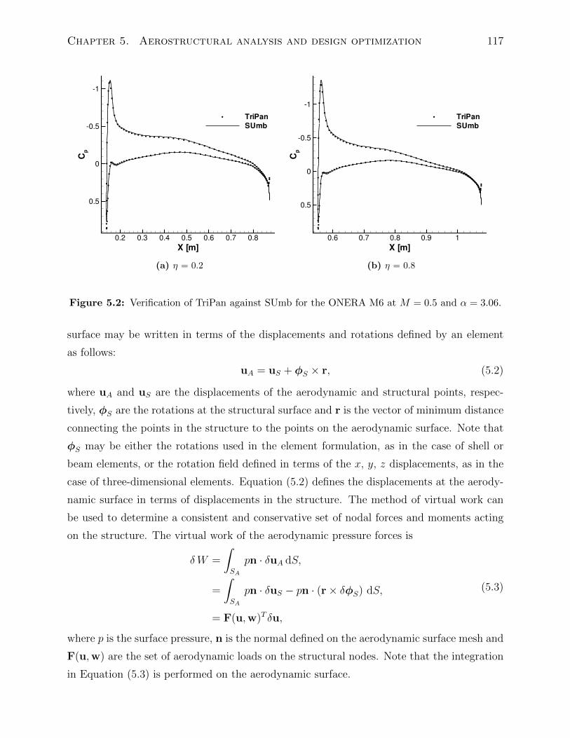
Chapter 5. Aerostructural analysis and design optimization 117
X [m]
Cp
0.2 0.3 0.4 0.5 0.6 0.7 0.8
1
0.5
0
0.5
TriPan
SUmb
(a) η = 0.2
X [m]
Cp
0.6 0.7 0.8 0.9 1
1
0.5
0
0.5
TriPan
SUmb
(b) η = 0.8
Figure 5.2: Verification of TriPan against SUmb for the ONERA M6 at M = 0.5 and α = 3.06.
surface may be written in terms of the displacements and rotations defined by an element
as follows:
uA = uS + φS × r, (5.2)
where uA and uS are the displacements of the aerodynamic and structural points, respec-
tively, φS are the rotations at the structural surface and r is the vector of minimum distance
connecting the points in the structure to the points on the aerodynamic surface. Note that
φS may be either the rotations used in the element formulation, as in the case of shell or
beam elements, or the rotation field defined in terms of the x, y, z displacements, as in the
case of three-dimensional elements. Equation (5.2) defines the displacements at the aerody-
namic surface in terms of displacements in the structure. The method of virtual work can
be used to determine a consistent and conservative set of nodal forces and moments acting
on the structure. The virtual work of the aerodynamic pressure forces is
δ W =
∫SA
pn · δuA dS,
=
∫SA
pn · δuS − pn · (r× δφS) dS,
= F(u,w)T δu,
(5.3)
where p is the surface pressure, n is the normal defined on the aerodynamic surface mesh and
F(u,w) are the set of aerodynamic loads on the structural nodes. Note that the integration
in Equation (5.3) is performed on the aerodynamic surface.
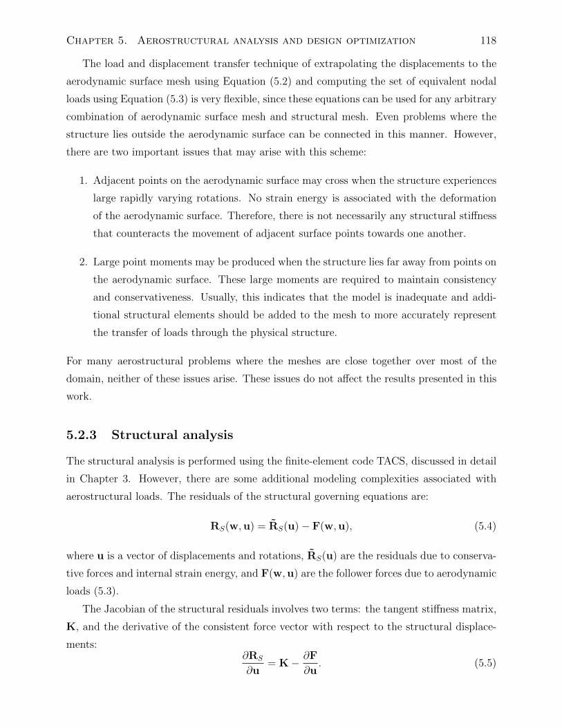
Chapter 5. Aerostructural analysis and design optimization 118
The load and displacement transfer technique of extrapolating the displacements to the
aerodynamic surface mesh using Equation (5.2) and computing the set of equivalent nodal
loads using Equation (5.3) is very flexible, since these equations can be used for any arbitrary
combination of aerodynamic surface mesh and structural mesh. Even problems where the
structure lies outside the aerodynamic surface can be connected in this manner. However,
there are two important issues that may arise with this scheme:
1. Adjacent points on the aerodynamic surface may cross when the structure experiences
large rapidly varying rotations. No strain energy is associated with the deformation
of the aerodynamic surface. Therefore, there is not necessarily any structural stiffness
that counteracts the movement of adjacent surface points towards one another.
2. Large point moments may be produced when the structure lies far away from points on
the aerodynamic surface. These large moments are required to maintain consistency
and conservativeness. Usually, this indicates that the model is inadequate and addi-
tional structural elements should be added to the mesh to more accurately represent
the transfer of loads through the physical structure.
For many aerostructural problems where the meshes are close together over most of the
domain, neither of these issues arise. These issues do not affect the results presented in this
work.
5.2.3 Structural analysis
The structural analysis is performed using the finite-element code TACS, discussed in detail
in Chapter 3. However, there are some additional modeling complexities associated with
aerostructural loads. The residuals of the structural governing equations are:
RS(w,u) = RS(u)− F(w,u), (5.4)
where u is a vector of displacements and rotations, RS(u) are the residuals due to conserva-
tive forces and internal strain energy, and F(w,u) are the follower forces due to aerodynamic
loads (5.3).
The Jacobian of the structural residuals involves two terms: the tangent stiffness matrix,
K, and the derivative of the consistent force vector with respect to the structural displace-
ments:∂RS
∂u= K− ∂F
∂u. (5.5)
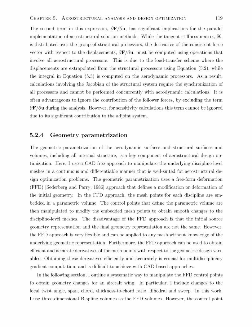
Chapter 5. Aerostructural analysis and design optimization 119
The second term in this expression, ∂F/∂u, has significant implications for the parallel
implementation of aerostructural solution methods. While the tangent stiffness matrix, K,
is distributed over the group of structural processors, the derivative of the consistent force
vector with respect to the displacements, ∂F/∂u, must be computed using operations that
involve all aerostructural processors. This is due to the load-transfer scheme where the
displacements are extrapolated from the structural processors using Equation (5.2), while
the integral in Equation (5.3) is computed on the aerodynamic processors. As a result,
calculations involving the Jacobian of the structural system require the synchronization of
all processors and cannot be performed concurrently with aerodynamic calculations. It is
often advantageous to ignore the contribution of the follower forces, by excluding the term
∂F/∂u during the analysis. However, for sensitivity calculations this term cannot be ignored
due to its significant contribution to the adjoint system.
5.2.4 Geometry parametrization
The geometric parametrization of the aerodynamic surfaces and structural surfaces and
volumes, including all internal structure, is a key component of aerostructural design op-
timization. Here, I use a CAD-free approach to manipulate the underlying discipline-level
meshes in a continuous and differentiable manner that is well-suited for aerostructural de-
sign optimization problems. The geometric parametrization uses a free-form deformation
(FFD) [Sederberg and Parry, 1986] approach that defines a modification or deformation of
the initial geometry. In the FFD approach, the mesh points for each discipline are em-
bedded in a parametric volume. The control points that define the parametric volume are
then manipulated to modify the embedded mesh points to obtain smooth changes to the
discipline-level meshes. The disadvantage of the FFD approach is that the initial source
geometry representation and the final geometry representation are not the same. However,
the FFD approach is very flexible and can be applied to any mesh without knowledge of the
underlying geometric representation. Furthermore, the FFD approach can be used to obtain
efficient and accurate derivatives of the mesh points with respect to the geometric design vari-
ables. Obtaining these derivatives efficiently and accurately is crucial for multidisciplinary
gradient computation, and is difficult to achieve with CAD-based approaches.
In the following section, I outline a systematic way to manipulate the FFD control points
to obtain geometry changes for an aircraft wing. In particular, I include changes to the
local twist angle, span, chord, thickness-to-chord ratio, dihedral and sweep. In this work,
I use three-dimensional B-spline volumes as the FFD volumes. However, the control point
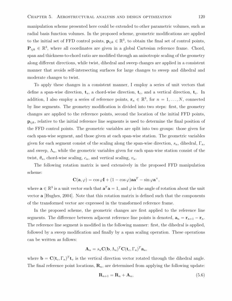
Chapter 5. Aerostructural analysis and design optimization 120
manipulation scheme presented here could be extended to other parametric volumes, such as
radial basis function volumes. In the proposed scheme, geometric modifications are applied
to the initial set of FFD control points, pijk ∈ R3, to obtain the final set of control points,
Pijk ∈ R3, where all coordinates are given in a global Cartesian reference frame. Chord,
span and thickness-to-chord ratio are modified through an anisotropic scaling of the geometry
along different directions, while twist, dihedral and sweep changes are applied in a consistent
manner that avoids self-intersecting surfaces for large changes to sweep and dihedral and
moderate changes to twist.
To apply these changes in a consistent manner, I employ a series of unit vectors that
define a span-wise direction, ts, a chord-wise direction, tc, and a vertical direction, tv. In
addition, I also employ a series of reference points, rn ∈ R3, for n = 1, . . . , N , connected
by line segments. The geometry modification is divided into two steps: first, the geometry
changes are applied to the reference points, second the location of the initial FFD points,
pijk, relative to the initial reference line segments is used to determine the final position of
the FFD control points. The geometric variables are split into two groups: those given for
each span-wise segment, and those given at each span-wise station. The geometric variables
given for each segment consist of the scaling along the span-wise direction, sn, dihedral, Γn,
and sweep, Λn, while the geometric variables given for each span-wise station consist of the
twist, θn, chord-wise scaling, cn, and vertical scaling, vn.
The following rotation matrix is used extensively in the proposed FFD manipulation
scheme:
C(a, ϕ) = cosϕI + (1− cosϕ)aaT − sinϕa×,
where a ∈ R3 is a unit vector such that aTa = 1, and ϕ is the angle of rotation about the unit
vector a [Hughes, 2004]. Note that this rotation matrix is defined such that the components
of the transformed vector are expressed in the transformed reference frame.
In the proposed scheme, the geometric changes are first applied to the reference line
segments. The difference between adjacent reference line points is denoted, an = rn+1 − rn.
The reference line segment is modified in the following manner: first, the dihedral is applied,
followed by a sweep modification and finally by a span scaling operation. These operations
can be written as follows:
An = snC(b,Λn)TC(tc,Γn)Tan,
where b = C(tc,Γn)T tv is the vertical direction vector rotated through the dihedral angle.
The final reference point locations, Rn, are determined from applying the following update:
Rn+1 = Rn + An, (5.6)
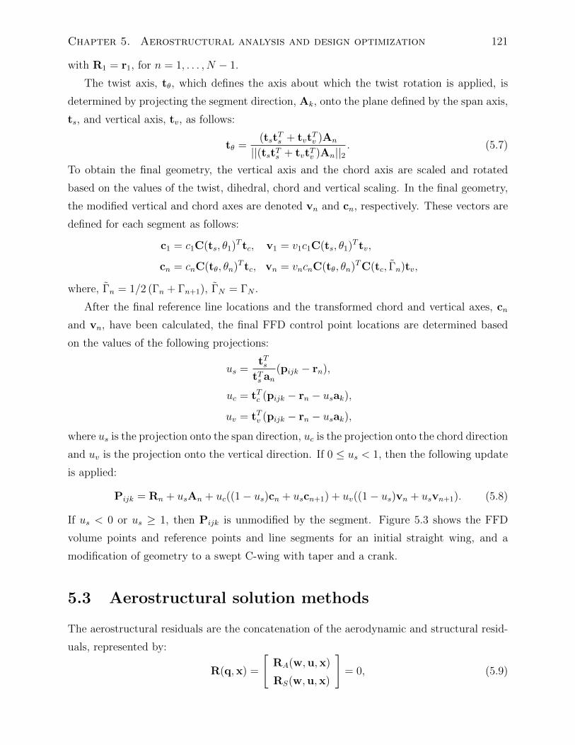
Chapter 5. Aerostructural analysis and design optimization 121
with R1 = r1, for n = 1, . . . , N − 1.
The twist axis, tθ, which defines the axis about which the twist rotation is applied, is
determined by projecting the segment direction, Ak, onto the plane defined by the span axis,
ts, and vertical axis, tv, as follows:
tθ =(tst
Ts + tvt
Tv )An
||(tstTs + tvtTv )An||2. (5.7)
To obtain the final geometry, the vertical axis and the chord axis are scaled and rotated
based on the values of the twist, dihedral, chord and vertical scaling. In the final geometry,
the modified vertical and chord axes are denoted vn and cn, respectively. These vectors are
defined for each segment as follows:
c1 = c1C(ts, θ1)T tc, v1 = v1c1C(ts, θ1)T tv,
cn = cnC(tθ, θn)T tc, vn = vncnC(tθ, θn)TC(tc, Γn)tv,
where, Γn = 1/2 (Γn + Γn+1), ΓN = ΓN .
After the final reference line locations and the transformed chord and vertical axes, cn
and vn, have been calculated, the final FFD control point locations are determined based
on the values of the following projections:
us =tTs
tTs an(pijk − rn),
uc = tTc (pijk − rn − usak),uv = tTv (pijk − rn − usak),
where us is the projection onto the span direction, uc is the projection onto the chord direction
and uv is the projection onto the vertical direction. If 0 ≤ us < 1, then the following update
is applied:
Pijk = Rn + usAn + uc((1− us)cn + uscn+1) + uv((1− us)vn + usvn+1). (5.8)
If us < 0 or us ≥ 1, then Pijk is unmodified by the segment. Figure 5.3 shows the FFD
volume points and reference points and line segments for an initial straight wing, and a
modification of geometry to a swept C-wing with taper and a crank.
5.3 Aerostructural solution methods
The aerostructural residuals are the concatenation of the aerodynamic and structural resid-
uals, represented by:
R(q,x) =
[RA(w,u,x)
RS(w,u,x)
]= 0, (5.9)
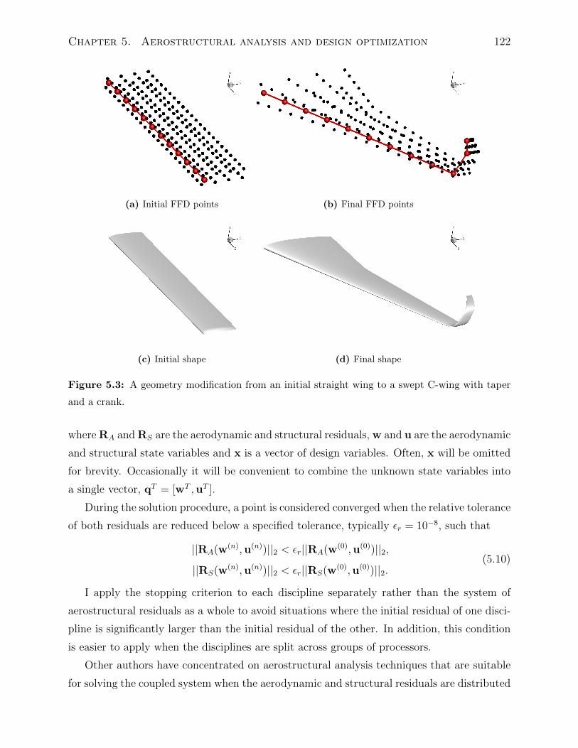
Chapter 5. Aerostructural analysis and design optimization 122
(a) Initial FFD points (b) Final FFD points
(c) Initial shape (d) Final shape
Figure 5.3: A geometry modification from an initial straight wing to a swept C-wing with taper
and a crank.
where RA and RS are the aerodynamic and structural residuals, w and u are the aerodynamic
and structural state variables and x is a vector of design variables. Often, x will be omitted
for brevity. Occasionally it will be convenient to combine the unknown state variables into
a single vector, qT = [wT ,uT ].
During the solution procedure, a point is considered converged when the relative tolerance
of both residuals are reduced below a specified tolerance, typically εr = 10−8, such that
||RA(w(n),u(n))||2 < εr||RA(w(0),u(0))||2,||RS(w(n),u(n))||2 < εr||RS(w(0),u(0))||2.
(5.10)
I apply the stopping criterion to each discipline separately rather than the system of
aerostructural residuals as a whole to avoid situations where the initial residual of one disci-
pline is significantly larger than the initial residual of the other. In addition, this condition
is easier to apply when the disciplines are split across groups of processors.
Other authors have concentrated on aerostructural analysis techniques that are suitable
for solving the coupled system when the aerodynamic and structural residuals are distributed
Chapter 5. Aerostructural analysis and design optimization 123
across the same set of processors, or the structural residuals are on every processor [Martins
et al., 2004, Barcelos and Maute, 2008]. Here, I focus on the situation where either memory
or performance requirements dictate that the aerodynamic and structural solvers be split
between groups of processors. This requires an additional level of parallelism reflected in the
solution algorithm.
In the following sections I present two variants of an approximate Newton–Krylov solution
algorithm. A more thorough investigation of other aerostructural solution algorithms is
presented in Kennedy and Martins [2010] where it is demonstrated that the approximate
Newton–Krylov approach is faster and more robust than either the block-Jacobi or Gauss–
Seidel methods.
5.3.1 Approximate Newton–Krylov methods
Newton’s method applied to Equation (5.9) results in the following linear system of equations
for the update ∆q(n),∂R
∂q∆q(n) = −R(q(n)). (5.11)
Newton’s method converges quadratically provided the starting point is sufficiently close to
the solution and the Jacobian remains non-singular. In order to achieve convergence from
points far from the solution, Newton’s method is often globalized with some strategy to
ensure progress is made towards the solution until a suitable starting point is found. I have
found, however, that globalization is not necessary for the aerostructural system (5.9).
In the Newton–Krylov approach, the linearized system (5.11) is solved inexactly using
a Krylov subspace method. The advantage of Krylov subspace methods is that they can
be constructed using only vector operations, matrix-vector products and a preconditioner
operator. In order to obtain an aerostructural solution method that is independent of the
details of the discipline-level solvers, I use a preconditioner based on generic discipline-level
preconditioners. Furthermore, I have implemented the off-diagonal matrix-vector products
and transpose matrix-vector products using a product-rule implementation [Kennedy and
Martins, 2010].
Many authors have used Jacobian-free Newton–Krylov methods where the matrix-vector
products are calculated using a finite-difference calculation. These techniques have been
applied successfully to many nonlinear problems [Knoll and Keyes, 2004]. However, for this
analysis, the formation of the aerodynamic residuals in TriPan is almost as costly as calcu-
lating the exact aerodynamic Jacobian, therefore, I have employed an exact computation of
the block-diagonal components of the aerostructural Jacobian.
Chapter 5. Aerostructural analysis and design optimization 124
Solving Equation (5.11) inexactly is typically more computationally efficient than finding
an accurate solution. Here, I solve the Newton update to a tolerance of εnk = 10−3, and
apply the stopping criterion:
||R(q(n)) +∂R
∂q∆q(n)||2 < εnk||R(q(n))||2, (5.12)
with the update q(n+1) = q(n)+∆q(n). I use the following stopping criterion, for the Newton–
Krylov methods:
||R(q(n))||2 < εrmin(||RA(q(0))||2, ||RS(q(0))||2). (5.13)
The treatment of the off-diagonal blocks requires a more detailed discussion. Since, a
Krylov approach is used to solve the linearized system of equations, only matrix-vector prod-
ucts are required for the linearization of the coupling terms. In the present implementation,
I compute the matrix-vector product [∂RA/∂u] v as the product of two terms:
∂RA
∂uv =
∂RA
∂Xs
∂Xs
∂uv, (5.14)
where Xs are the aerodynamic nodal locations, and v is an arbitrary vector. Note that the
first term, ∂RA/∂Xs, is computed on the aerodynamic processors, while the second term
∂Xs/∂u is computed on the structural processors.
The first term in Equation (5.14), ∂RA/∂Xs, is a dense matrix that is fully populated
due to the nature of the panel method. This term is also required for the adjoint system of
equations. The formation of ∂RA/∂Xs is a time consuming operation, typically requiring
20 to 50 times the computational time of forming the aerodynamic residuals. As a result,
I do not recalculate this term at every iteration. Instead, I recompute ∂RA/∂Xs when
mod(n,m) = 0 for m = 10. This high value of m is chosen since I have found that the
Newton updates computed in this manner are effective, and that for the best computational
performance, ∂RA/∂Xs should be updated only if the aerostructural problem is difficult to
solve. This modification renders this algorithm an approximate Newton method since the
exact Jacobian is formed only every mth iteration. I label this variant of the approximate
Newton–Krylov method ANK 1.
I have found that the ANK 1 method is robust, but that the high-cost of forming
∂RA/∂Xs makes ANK 1 significantly slower than the nonlinear block Gauss–Seidel ap-
proach. In order to achieve better computational performance, I have implemented a method
to approximate the term ∂RA/∂Xs within the aerodynamic code. This approximation is
constructed by computing the contributions from panels only within a given radius of one
Chapter 5. Aerostructural analysis and design optimization 125
another, in a manner analogous to the technique used to form the aerodynamic precondi-
tioner. This reduces the computational cost of this term significantly. I label this second
variant of the approximate Newton–Krylov method ANK 2.
The matrix-vector products with the other off-diagonal block [∂RS/∂w] s, are calculated
using the following series of operations:
∂RS
∂ws =
∂RS
∂fA
∂fA∂w
s = − ∂F
∂fA
∂fA∂w
s, (5.15)
where fA is a vector of the integrated forces over the aerodynamic surface. Note that the
term ∂fA/∂w is formed on the aerodynamic processors, while the term ∂RS/∂fA is computed
on the structural processors. The product of these terms is implemented using a matrix-
free approach in which the matrix components are computed and discarded each time a
matrix-vector product is computed.
At each iteration, I approximately solve the Newton update (5.11), using preconditioned
F-GMRES(60) [Saad, 1993]. The preconditioner is based on a single application of block
Jacobi. In this approach, each discipline applies a block-preconditioner to its own set of
equations. I have found that an effective approach is to use GMRES(5) for the aerodynamic
processors, and one application of the structural preconditioner — usually the direct Schur
method discussed in Section 3.3.2. This set of preconditioning options is set to approximately
balance the time required for the aerodynamic and structural preconditioning operations for
typical problem sizes.
5.3.2 Aerostructural analysis performance
In this section, I examine the parallel performance of the aerostructural solution algorithms
described in the previous section. The results presented here are based on calculations
performed on the GPC at SciNet [Loken et al., 2010] (see Section 3.3.3 for a more detailed
description of SciNet’s configuration.)
I assess the parallel solution performance of the ANK 1 and ANK 2 algorithms for an
aerostructural system consisting of a finite-element structural model that contains 1.6 million
degrees of freedom, and an aerodynamic model that contains 14 440 surface panels and 18 000
wake panels. Figure 5.4 shows the solution times for test cases run with 16, 24, 32, 48, and 64
processors for a stiff structure with a span of b = 60.9 m, and a flexible structure with a span
of b = 81.0 m. For all cases the processors were divided evenly amongst the structural and
aerodynamic process groups. Both the ANK 1 and ANK 2 algorithms exhibit good parallel
scalability. The ANK 2 method performs roughly 1.5 times faster than the ANK 1 method for
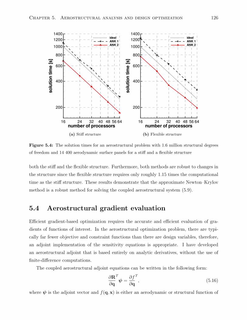
Chapter 5. Aerostructural analysis and design optimization 126
number of processors
solutiontime[s]
16 24 32 40 48 56 64
200
400
600
800
1000
1200
1400ideal
ANK 1
ANK 2
(a) Stiff structure
number of processorssolutiontime[s]
16 24 32 40 48 56 64
200
400
600
800
1000
1200
1400ideal
ANK 1
ANK 2
(b) Flexible structure
Figure 5.4: The solution times for an aerostructural problem with 1.6 million structural degrees
of freedom and 14 400 aerodynamic surface panels for a stiff and a flexible structure
both the stiff and the flexible structure. Furthermore, both methods are robust to changes in
the structure since the flexible structure requires only roughly 1.15 times the computational
time as the stiff structure. These results demonstrate that the approximate Newton–Krylov
method is a robust method for solving the coupled aerostructural system (5.9).
5.4 Aerostructural gradient evaluation
Efficient gradient-based optimization requires the accurate and efficient evaluation of gra-
dients of functions of interest. In the aerostructural optimization problem, there are typi-
cally far fewer objective and constraint functions than there are design variables, therefore,
an adjoint implementation of the sensitivity equations is appropriate. I have developed
an aerostructural adjoint that is based entirely on analytic derivatives, without the use of
finite-difference computations.
The coupled aerostructural adjoint equations can be written in the following form:
∂R
∂q
T
ψ =∂f
∂q
T
, (5.16)
where ψ is the adjoint vector and f(q,x) is either an aerodynamic or structural function of
Chapter 5. Aerostructural analysis and design optimization 127
interest. The total derivative is determined using the additional computation:
∇xf =∂f
∂x−ψT ∂R
∂x. (5.17)
I have implemented the adjoint sensitivity method for aerodynamic lift, drag and moments,
as well as the Kreisselmeier–Steinhauser (KS) function of the structural failure criteria and
buckling envelope.
I use a Krylov method to solve the linear coupled aerostructural adjoint equations (5.16).
In the Krylov approach, the matrix-vector products are computed using the exact Jacobian-
transpose of the coupled aerostructural system. One iteration of a transpose block Jacobi
iteration is used as the preconditioner, with similar settings to those used in the Newton–
Krylov solution method. The adjoint equations are solved to a relative tolerance of εrA =
10−10.
Once the adjoint vector ψ has been determined, the total sensitivities must be computed
using Equation (5.17). This calculation requires the partial derivative of the residuals with
respect to the design variables. I have implemented the aerostructural adjoint equations with
geometric, structural and angle of attack design variables. The geometric design variables
are the most costly to compute, requiring the following calculations:
ψTA
∂RA
∂x= ψT
A
∂RA
∂Xs
∂Xs
∂x, (5.18)
ψTS
∂RS
∂x= ψT
S
∂RS
∂x−ψT
S
∂F
∂fA
∂fA∂Xs
∂Xs
∂x. (5.19)
These computations must again take into consideration the distribution of the disciplines
across multiple process groups. Equation (5.18) involves terms only on the aerodynamic pro-
cesses, while Equation (5.19) involves terms on both structural and aerodynamic processes.
As a result, this operation requires significantly more communication.
5.4.1 Sensitivity performance study
Figure 5.5 shows the results of a sensitivity parallel scalability test run on 16, 24, 32, 48,
and 64 processors. The aerostructural model is the same as that described in Section 5.3.2.
The timing results are shown for both the Trefftz plane drag function and the KS failure
function, and the time required to compute ∂RA/∂Xs and other terms required for the
adjoint sensitivity computations labeled “adjoint set up” time. Note that these adjoint terms
can be reused for each gradient evaluation at the given values of the state variables. Thus,
the adjoint set up time can be amortized over the different gradient evaluations. Figure 5.5
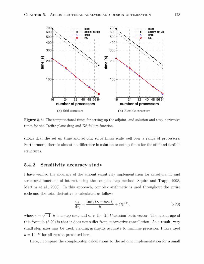
Chapter 5. Aerostructural analysis and design optimization 128
number of processors
time[s]
16 24 32 40 48 56 64
100
200
300
400
500
600
700 ideal
adjoint set up
drag
KS
(a) Stiff structure
number of processorstime[s]
16 24 32 40 48 56 64
100
200
300
400
500
600
700 ideal
adjoint set up
drag
KS
(b) Flexible structure
Figure 5.5: The computational times for setting up the adjoint, and solution and total derivative
times for the Trefftz plane drag and KS failure function.
shows that the set up time and adjoint solve times scale well over a range of processors.
Furthermore, there is almost no difference in solution or set up times for the stiff and flexible
structures.
5.4.2 Sensitivity accuracy study
I have verified the accuracy of the adjoint sensitivity implementation for aerodynamic and
structural functions of interest using the complex-step method [Squire and Trapp, 1998,
Martins et al., 2003]. In this approach, complex arithmetic is used throughout the entire
code and the total derivative is calculated as follows:
df
dxi=
Im(f(x + ihei))
h+O(h2), (5.20)
where i =√−1, h is a step size, and ei is the ith Cartesian basis vector. The advantage of
this formula (5.20) is that it does not suffer from subtractive cancellation. As a result, very
small step sizes may be used, yielding gradients accurate to machine precision. I have used
h = 10−30 for all results presented here.
Here, I compare the complex-step calculations to the adjoint implementation for a small
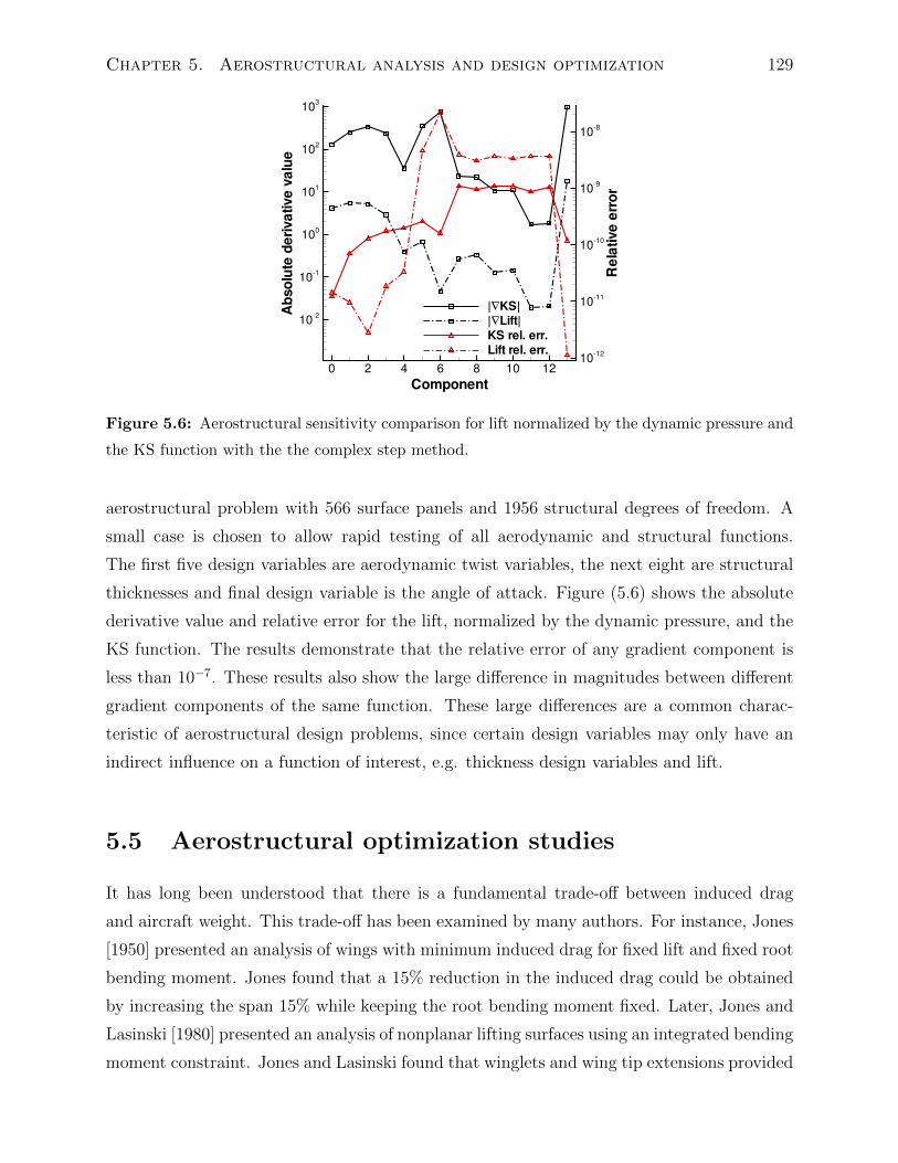
Chapter 5. Aerostructural analysis and design optimization 129
Component
Absolute
derivativevalue
Relativeerror
0 2 4 6 8 10 12
102
101
100
101
102
103
1012
1011
1010
109
108
|∇KS|
|∇Lift|
KS rel. err.
Lift rel. err.
Figure 5.6: Aerostructural sensitivity comparison for lift normalized by the dynamic pressure and
the KS function with the the complex step method.
aerostructural problem with 566 surface panels and 1956 structural degrees of freedom. A
small case is chosen to allow rapid testing of all aerodynamic and structural functions.
The first five design variables are aerodynamic twist variables, the next eight are structural
thicknesses and final design variable is the angle of attack. Figure (5.6) shows the absolute
derivative value and relative error for the lift, normalized by the dynamic pressure, and the
KS function. The results demonstrate that the relative error of any gradient component is
less than 10−7. These results also show the large difference in magnitudes between different
gradient components of the same function. These large differences are a common charac-
teristic of aerostructural design problems, since certain design variables may only have an
indirect influence on a function of interest, e.g. thickness design variables and lift.
5.5 Aerostructural optimization studies
It has long been understood that there is a fundamental trade-off between induced drag
and aircraft weight. This trade-off has been examined by many authors. For instance, Jones
[1950] presented an analysis of wings with minimum induced drag for fixed lift and fixed root
bending moment. Jones found that a 15% reduction in the induced drag could be obtained
by increasing the span 15% while keeping the root bending moment fixed. Later, Jones and
Lasinski [1980] presented an analysis of nonplanar lifting surfaces using an integrated bending
moment constraint. Jones and Lasinski found that winglets and wing tip extensions provided
Chapter 5. Aerostructural analysis and design optimization 130
approximately equal reduction in the induced drag for a given integrated bending moment
constraint. More recently, Ning and Kroo [2010] performed an analysis and optimization
of wings with various wing tip devices. They used a calibrated weight model that included
an integrated bending moment calculation and a historical weight correlation to predict the
relative changes in weight of different designs from a baseline configuration.
Other studies have used structural analysis techniques to obtain the flying shape of the
wing, and to size a portion of the aircraft structure and thus predict a partial wing-weight. In
one of the earliest examples of aerostructural optimization, Haftka [1977] compared the trade-
off between structural weight and induced drag for both composite and isotropic wings of a
fighter aircraft. Haftka obtained the displaced shape through an iterative procedure and used
stress constraints to size the aircraft wing skins. More recently, Jansen et al. [2010] presented
optimizations of various nonplanar configurations using a gradient-free optimization method.
They used a calibrated lifting line method to predict both induced and viscous drag, and
analyzed all configurations in the displaced, flying shape.
In this work, I examine aerostructural induced drag minimization of a transonic transport
wing. Induced drag, or drag due to lift, is a portion of the drag that can be attributed to the
generation of lift [Kroo, 2000]. The induced drag, Di, can be computed using the following
formula:
Di =L2
πqb2e, (5.21)
where L is the lift, q is the dynamic pressure, b is the span, and e is the span efficiency
factor. In a steady, level flight condition the lift generated by the aircraft is equal to the
total aircraft weight, L = W . As a result, there is a trade-off between decreasing the induced
drag by increasing the span, b, leading to higher overall structural weight, and decreasing
the structural weight of the wing leading to overall lower aircraft weight. Based on a simple
analysis presented by Kroo [2000], this trade-off occurs when the wing-weight is roughly 1/3
of the aircraft weight. Typical transport aircraft wings constitute closer to 10% of maximum
takeoff weight (MTOW), and are far from the region where this trade-off becomes active.
Instead, more practical aircraft design objectives, such as fuel burn, place a larger emphasis
on structural weight than an analysis of Equation (5.21) would suggest.
In order to focus on the trade-off between induced drag and wing weight, and obtain
designs that have a reasonable span, I include a target mass constraint within the aerostruc-
tural optimization problem. The target mass is set as a fraction of the structural mass of a
wing obtained from a structural optimization under fixed aerodynamic loads. The results of
aerostructural optimizations for different target masses are examined below. In addition, in
Chapter 5. Aerostructural analysis and design optimization 131
order to constrain the viscous drag, I impose a wetted area constraint such that the initial
and final wetted areas must be equal. This constraint does not account for higher-order vis-
cous drag effects due to variation in slenderness ratio or Reynolds number, but does provide
a useful starting point for comparison purposes.
The geometry for all cases presented below is based on a Boeing 777-200 aircraft wing
with an initial span of 60.9 m, a taper ratio of 0.2, and a root chord of 13.2 m. The wing
crank is set at 30% of the semi-span. The initial wing is a linear loft of RAE2822 airfoil
sections, without twist or dihedral. The wetted surface area of the wing is 837.47 m2. The
wing structure consists of 44 equally spaced chord-wise ribs, with front and rear spars located
at 10% and 70% chord offset from the leading edge, respectively. The leading and trailing
edge structure is not modeled. The aerodynamic mesh consists of 4200 surface mesh panels:
60 span-wise panels and 70 chord-wise panels, with 100 stream-wise wake panels for each
trailing edge panel. The structural model consists of 29 216 3rd order, MITC9 shell elements
with a total of 114 556 nodes and just over 687 000 degrees of freedom.
The aerostructural optimization problem consists of an on-design cruise flight condition,
and two maneuver conditions used to size the wing-box: a 2.5g maneuver condition and a
-1g maneuver condition. The cruise condition is calculated at a Mach number of 0.84 at an
altitude of 10 688 m, or 35 000 ft. The maneuver conditions are calculated at an altitude
of 4000 m or approximately 13 100 ft, at a Mach number of 0.9 in order to represent a dive
condition at low altitude. Standard atmospheric conditions are used at these altitudes. The
maneuver flight conditions at this low altitude and high Mach number are possible without
stalling the wing. Within the context of the optimization problem, the angles of attack at
these flight conditions are considered design variables. In all cases, the MTOW of the aircraft
is 297 550 kg. The cruise condition is calculated at mcruise = MTOW − 1/2mfuel, where
mfuel = 171 175 kg, while the maneuver conditions are calculated at MTOW. No inertial
relief from the fuel or self-weight of the structure is included in the calculations presented
here, but should be considered in future work. Note that the Mach numbers at the cruise and
maneuver flight conditions are beyond the range of validity of the Prandlt–Glauert equation,
and future work should consider the use of at least Euler CFD methods. However, using
lower Mach numbers, within a range suitable for the panel method, would lead to high
cruise and maneuver CL values, which would result in unrealistically large sectional pitching
moments at the maneuver conditions.
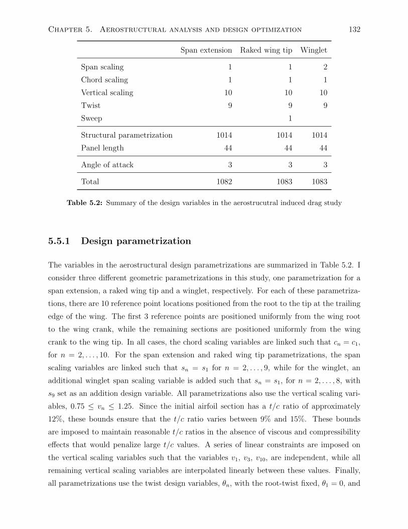
Chapter 5. Aerostructural analysis and design optimization 132
Span extension Raked wing tip Winglet
Span scaling 1 1 2
Chord scaling 1 1 1
Vertical scaling 10 10 10
Twist 9 9 9
Sweep 1
Structural parametrization 1014 1014 1014
Panel length 44 44 44
Angle of attack 3 3 3
Total 1082 1083 1083
Table 5.2: Summary of the design variables in the aerostrucutral induced drag study
5.5.1 Design parametrization
The variables in the aerostructural design parametrizations are summarized in Table 5.2. I
consider three different geometric parametrizations in this study, one parametrization for a
span extension, a raked wing tip and a winglet, respectively. For each of these parametriza-
tions, there are 10 reference point locations positioned from the root to the tip at the trailing
edge of the wing. The first 3 reference points are positioned uniformly from the wing root
to the wing crank, while the remaining sections are positioned uniformly from the wing
crank to the wing tip. In all cases, the chord scaling variables are linked such that cn = c1,
for n = 2, . . . , 10. For the span extension and raked wing tip parametrizations, the span
scaling variables are linked such that sn = s1 for n = 2, . . . , 9, while for the winglet, an
additional winglet span scaling variable is added such that sn = s1, for n = 2, . . . , 8, with
s9 set as an addition design variable. All parametrizations also use the vertical scaling vari-
ables, 0.75 ≤ vn ≤ 1.25. Since the initial airfoil section has a t/c ratio of approximately
12%, these bounds ensure that the t/c ratio varies between 9% and 15%. These bounds
are imposed to maintain reasonable t/c ratios in the absence of viscous and compressibility
effects that would penalize large t/c values. A series of linear constraints are imposed on
the vertical scaling variables such that the variables v1, v3, v10, are independent, while all
remaining vertical scaling variables are interpolated linearly between these values. Finally,
all parametrizations use the twist design variables, θn, with the root-twist fixed, θ1 = 0, and
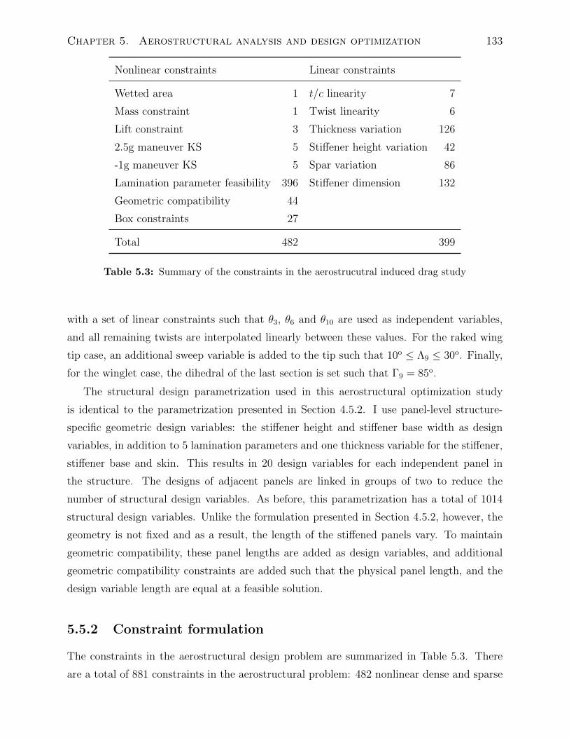
Chapter 5. Aerostructural analysis and design optimization 133
Nonlinear constraints Linear constraints
Wetted area 1 t/c linearity 7
Mass constraint 1 Twist linearity 6
Lift constraint 3 Thickness variation 126
2.5g maneuver KS 5 Stiffener height variation 42
-1g maneuver KS 5 Spar variation 86
Lamination parameter feasibility 396 Stiffener dimension 132
Geometric compatibility 44
Box constraints 27
Total 482 399
Table 5.3: Summary of the constraints in the aerostrucutral induced drag study
with a set of linear constraints such that θ3, θ6 and θ10 are used as independent variables,
and all remaining twists are interpolated linearly between these values. For the raked wing
tip case, an additional sweep variable is added to the tip such that 10o ≤ Λ9 ≤ 30o. Finally,
for the winglet case, the dihedral of the last section is set such that Γ9 = 85o.
The structural design parametrization used in this aerostructural optimization study
is identical to the parametrization presented in Section 4.5.2. I use panel-level structure-
specific geometric design variables: the stiffener height and stiffener base width as design
variables, in addition to 5 lamination parameters and one thickness variable for the stiffener,
stiffener base and skin. This results in 20 design variables for each independent panel in
the structure. The designs of adjacent panels are linked in groups of two to reduce the
number of structural design variables. As before, this parametrization has a total of 1014
structural design variables. Unlike the formulation presented in Section 4.5.2, however, the
geometry is not fixed and as a result, the length of the stiffened panels vary. To maintain
geometric compatibility, these panel lengths are added as design variables, and additional
geometric compatibility constraints are added such that the physical panel length, and the
design variable length are equal at a feasible solution.
5.5.2 Constraint formulation
The constraints in the aerostructural design problem are summarized in Table 5.3. There
are a total of 881 constraints in the aerostructural problem: 482 nonlinear dense and sparse
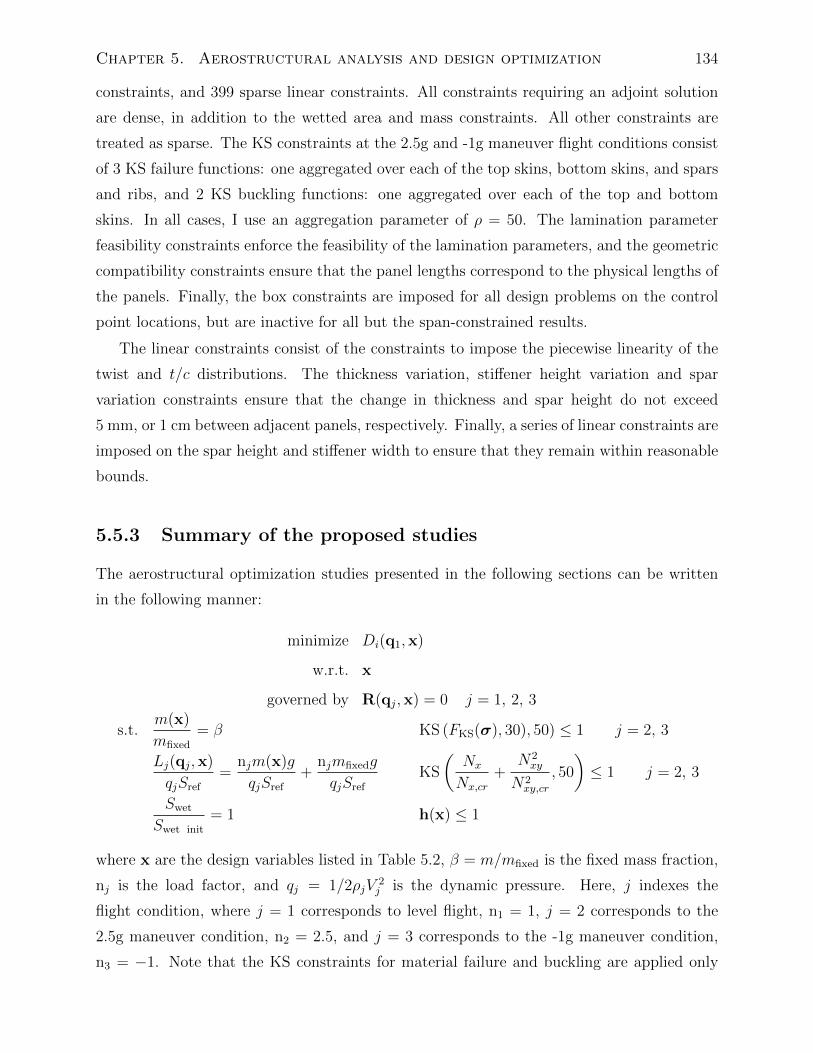
Chapter 5. Aerostructural analysis and design optimization 134
constraints, and 399 sparse linear constraints. All constraints requiring an adjoint solution
are dense, in addition to the wetted area and mass constraints. All other constraints are
treated as sparse. The KS constraints at the 2.5g and -1g maneuver flight conditions consist
of 3 KS failure functions: one aggregated over each of the top skins, bottom skins, and spars
and ribs, and 2 KS buckling functions: one aggregated over each of the top and bottom
skins. In all cases, I use an aggregation parameter of ρ = 50. The lamination parameter
feasibility constraints enforce the feasibility of the lamination parameters, and the geometric
compatibility constraints ensure that the panel lengths correspond to the physical lengths of
the panels. Finally, the box constraints are imposed for all design problems on the control
point locations, but are inactive for all but the span-constrained results.
The linear constraints consist of the constraints to impose the piecewise linearity of the
twist and t/c distributions. The thickness variation, stiffener height variation and spar
variation constraints ensure that the change in thickness and spar height do not exceed
5 mm, or 1 cm between adjacent panels, respectively. Finally, a series of linear constraints are
imposed on the spar height and stiffener width to ensure that they remain within reasonable
bounds.
5.5.3 Summary of the proposed studies
The aerostructural optimization studies presented in the following sections can be written
in the following manner:
minimize Di(q1,x)
w.r.t. x
governed by R(qj,x) = 0 j = 1, 2, 3
s.t.m(x)
mfixed
= β KS (FKS(σ), 30), 50) ≤ 1 j = 2, 3
Lj(qj,x)
qjSref
=njm(x)g
qjSref
+njmfixedg
qjSref
KS
(Nx
Nx,cr
+N2xy
N2xy,cr
, 50
)≤ 1 j = 2, 3
Swet
Swet init
= 1 h(x) ≤ 1
where x are the design variables listed in Table 5.2, β = m/mfixed is the fixed mass fraction,
nj is the load factor, and qj = 1/2ρjV2j is the dynamic pressure. Here, j indexes the
flight condition, where j = 1 corresponds to level flight, n1 = 1, j = 2 corresponds to the
2.5g maneuver condition, n2 = 2.5, and j = 3 corresponds to the -1g maneuver condition,
n3 = −1. Note that the KS constraints for material failure and buckling are applied only
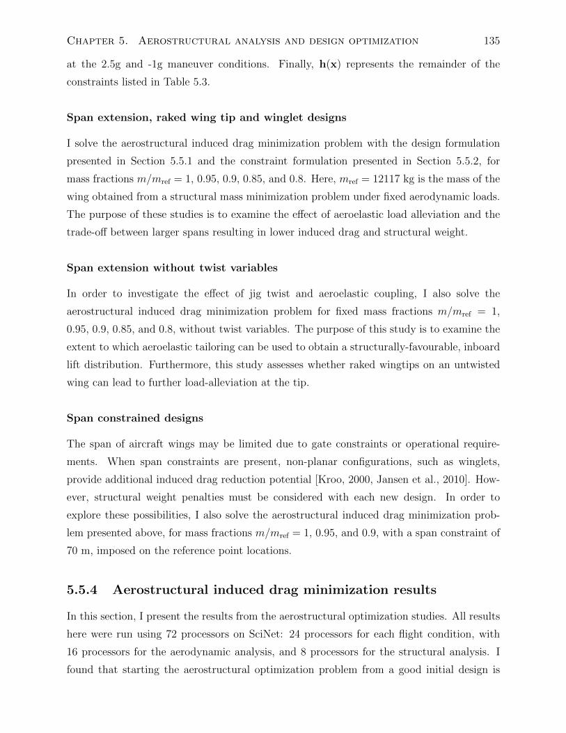
Chapter 5. Aerostructural analysis and design optimization 135
at the 2.5g and -1g maneuver conditions. Finally, h(x) represents the remainder of the
constraints listed in Table 5.3.
Span extension, raked wing tip and winglet designs
I solve the aerostructural induced drag minimization problem with the design formulation
presented in Section 5.5.1 and the constraint formulation presented in Section 5.5.2, for
mass fractions m/mref = 1, 0.95, 0.9, 0.85, and 0.8. Here, mref = 12117 kg is the mass of the
wing obtained from a structural mass minimization problem under fixed aerodynamic loads.
The purpose of these studies is to examine the effect of aeroelastic load alleviation and the
trade-off between larger spans resulting in lower induced drag and structural weight.
Span extension without twist variables
In order to investigate the effect of jig twist and aeroelastic coupling, I also solve the
aerostructural induced drag minimization problem for fixed mass fractions m/mref = 1,
0.95, 0.9, 0.85, and 0.8, without twist variables. The purpose of this study is to examine the
extent to which aeroelastic tailoring can be used to obtain a structurally-favourable, inboard
lift distribution. Furthermore, this study assesses whether raked wingtips on an untwisted
wing can lead to further load-alleviation at the tip.
Span constrained designs
The span of aircraft wings may be limited due to gate constraints or operational require-
ments. When span constraints are present, non-planar configurations, such as winglets,
provide additional induced drag reduction potential [Kroo, 2000, Jansen et al., 2010]. How-
ever, structural weight penalties must be considered with each new design. In order to
explore these possibilities, I also solve the aerostructural induced drag minimization prob-
lem presented above, for mass fractions m/mref = 1, 0.95, and 0.9, with a span constraint of
70 m, imposed on the reference point locations.
5.5.4 Aerostructural induced drag minimization results
In this section, I present the results from the aerostructural optimization studies. All results
here were run using 72 processors on SciNet: 24 processors for each flight condition, with
16 processors for the aerodynamic analysis, and 8 processors for the structural analysis. I
found that starting the aerostructural optimization problem from a good initial design is
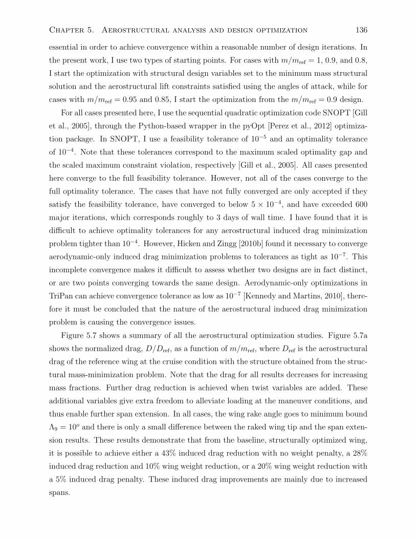
Chapter 5. Aerostructural analysis and design optimization 136
essential in order to achieve convergence within a reasonable number of design iterations. In
the present work, I use two types of starting points. For cases with m/mref = 1, 0.9, and 0.8,
I start the optimization with structural design variables set to the minimum mass structural
solution and the aerostructural lift constraints satisfied using the angles of attack, while for
cases with m/mref = 0.95 and 0.85, I start the optimization from the m/mref = 0.9 design.
For all cases presented here, I use the sequential quadratic optimization code SNOPT [Gill
et al., 2005], through the Python-based wrapper in the pyOpt [Perez et al., 2012] optimiza-
tion package. In SNOPT, I use a feasibility tolerance of 10−5 and an optimality tolerance
of 10−4. Note that these tolerances correspond to the maximum scaled optimality gap and
the scaled maximum constraint violation, respectively [Gill et al., 2005]. All cases presented
here converge to the full feasibility tolerance. However, not all of the cases converge to the
full optimality tolerance. The cases that have not fully converged are only accepted if they
satisfy the feasibility tolerance, have converged to below 5 × 10⁻⁴, and have exceeded 600
major iterations, which corresponds roughly to 3 days of wall time. I have found that it is
difficult to achieve optimality tolerances for any aerostructural induced drag minimization
problem tighter than 10−4. However, Hicken and Zingg [2010b] found it necessary to converge
aerodynamic-only induced drag minimization problems to tolerances as tight as 10−7. This
incomplete convergence makes it difficult to assess whether two designs are in fact distinct,
or are two points converging towards the same design. Aerodynamic-only optimizations in
TriPan can achieve convergence tolerance as low as 10−7 [Kennedy and Martins, 2010], there-
fore it must be concluded that the nature of the aerostructural induced drag minimization
problem is causing the convergence issues.
Figure 5.7 shows a summary of all the aerostructural optimization studies. Figure 5.7a
shows the normalized drag, D/Dref, as a function of m/mref, where Dref is the aerostructural
drag of the reference wing at the cruise condition with the structure obtained from the struc-
tural mass-minimization problem. Note that the drag for all results decreases for increasing
mass fractions. Further drag reduction is achieved when twist variables are added. These
additional variables give extra freedom to alleviate loading at the maneuver conditions, and
thus enable further span extension. In all cases, the wing rake angle goes to minimum bound
Λ9 = 10o and there is only a small difference between the raked wing tip and the span exten-
sion results. These results demonstrate that from the baseline, structurally optimized wing,
it is possible to achieve either a 43% induced drag reduction with no weight penalty, a 28%
induced drag reduction and 10% wing weight reduction, or a 20% wing weight reduction with
a 5% induced drag penalty. These induced drag improvements are mainly due to increased
spans.
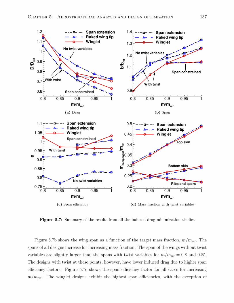
Chapter 5. Aerostructural analysis and design optimization 137
m/mref
D/D
ref
0.8 0.85 0.9 0.95 1
0.6
0.7
0.8
0.9
1
1.1
1.2 Span extension
Raked wing tip
Winglet
No twist variables
With twist
Span constrained
(a) Drag
m/mref
b/b
ref
0.8 0.85 0.9 0.95 1
0.9
1
1.1
1.2
1.3
1.4 Span extension
Raked wing tip
Winglet
No twist variables
Span constrained
With twist
(b) Span
m/mref
e
0.8 0.85 0.9 0.95 1
0.75
0.8
0.85
0.9
0.95
1
1.05
1.1 Span extension
Raked wing tip
Winglet
No twist variables
With twist
Span constrained
(c) Span efficiency
m/mref
mcomponent/m
ref
0.8 0.85 0.9 0.95 1
0.2
0.25
0.3
0.35
0.4
0.45
0.5 Span extension
Raked wing tip
Winglet
Top skin
Bottom skin
Ribs and spars
(d) Mass fraction with twist variables
Figure 5.7: Summary of the results from all the induced drag minimization studies
Figure 5.7b shows the wing span as a function of the target mass fraction, m/mref. The
spans of all designs increase for increasing mass fraction. The span of the wings without twist
variables are slightly larger than the spans with twist variables for m/mref = 0.8 and 0.85.
The designs with twist at these points, however, have lower induced drag due to higher span
efficiency factors. Figure 5.7c shows the span efficiency factor for all cases for increasing
m/mref. The winglet designs exhibit the highest span efficiencies, with the exception of
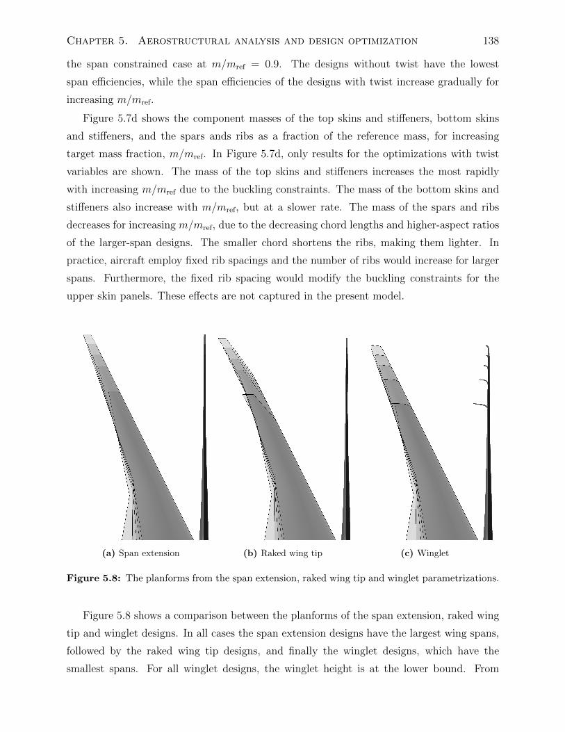
Chapter 5. Aerostructural analysis and design optimization 138
the span constrained case at m/mref = 0.9. The designs without twist have the lowest
span efficiencies, while the span efficiencies of the designs with twist increase gradually for
increasing m/mref.
Figure 5.7d shows the component masses of the top skins and stiffeners, bottom skins
and stiffeners, and the spars ands ribs as a fraction of the reference mass, for increasing
target mass fraction, m/mref. In Figure 5.7d, only results for the optimizations with twist
variables are shown. The mass of the top skins and stiffeners increases the most rapidly
with increasing m/mref due to the buckling constraints. The mass of the bottom skins and
stiffeners also increase with m/mref, but at a slower rate. The mass of the spars and ribs
decreases for increasing m/mref, due to the decreasing chord lengths and higher-aspect ratios
of the larger-span designs. The smaller chord shortens the ribs, making them lighter. In
practice, aircraft employ fixed rib spacings and the number of ribs would increase for larger
spans. Furthermore, the fixed rib spacing would modify the buckling constraints for the
upper skin panels. These effects are not captured in the present model.
(a) Span extension (b) Raked wing tip (c) Winglet
Figure 5.8: The planforms from the span extension, raked wing tip and winglet parametrizations.
Figure 5.8 shows a comparison between the planforms of the span extension, raked wing
tip and winglet designs. In all cases the span extension designs have the largest wing spans,
followed by the raked wing tip designs, and finally the winglet designs, which have the
smallest spans. For all winglet designs, the winglet height is at the lower bound. From
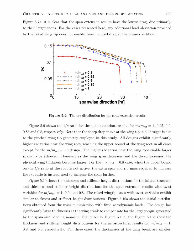
Chapter 5. Aerostructural analysis and design optimization 139
Figure 5.7a, it is clear that the span extension results have the lowest drag, due primarily
to their larger spans. For the cases presented here, any additional load aleviation provided
by the raked wing tip does not enable lower induced drag at the cruise condition.
spanwise direction [m]
t/c
0 10 20 30 400
0.05
0.1
0.15
m/mref
= 0.8
m/mref
= 0.85
m/mref
= 0.9
m/mref
= 0.95
m/mref
= 1
Figure 5.9: The t/c distribution for the span extension results
Figure 5.9 shows the t/c ratio for the span extensions results for m/mref = 1, 0.95, 0.9,
0.85 and 0.8, respectively. Note that the sharp drop in t/c at the wing tip in all designs is due
to the pinched wing tip geometry employed in this study. All designs exhibit significantly
higher t/c ratios near the wing root, reaching the upper bound at the wing root in all cases
except for the m/mref = 0.8 design. The higher t/c ratios near the wing root enable larger
spans to be achieved. However, as the wing span decreases and the chord increases, the
physical wing thickness becomes larger. For the m/mref = 0.8 case, when the upper bound
on the t/c ratio at the root is not active, the extra spar and rib mass required to increase
the t/c ratio is instead used to increase the span further.
Figure 5.10 shows the thickness and stiffener height distributions for the initial structure,
and thickness and stiffener height distributions for the span extension results with twist
variables for m/mref = 1, 0.9, and 0.8. The raked wingtip cases with twist variables exhibit
similar thickness and stiffener height distributions. Figure 5.10a shows the initial distribu-
tions obtained from the mass minimization with fixed aerodynamic loads. The design has
significantly large thicknesses at the wing crank to compensate for the large torque generated
by the span-wise bending moment. Figure 5.10b, Figure 5.10c, and Figure 5.10d show the
thickness and stiffener height distributions for the aerostructural results for m/mref = 1,
0.9, and 0.8, respectively. For these cases, the thicknesses at the wing break are smaller,
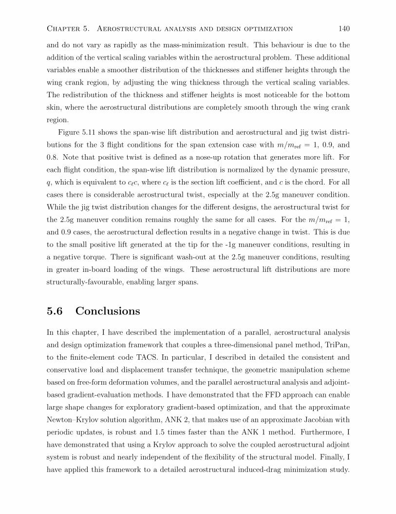
Chapter 5. Aerostructural analysis and design optimization 140
and do not vary as rapidly as the mass-minimization result. This behaviour is due to the
addition of the vertical scaling variables within the aerostructural problem. These additional
variables enable a smoother distribution of the thicknesses and stiffener heights through the
wing crank region, by adjusting the wing thickness through the vertical scaling variables.
The redistribution of the thickness and stiffener heights is most noticeable for the bottom
skin, where the aerostructural distributions are completely smooth through the wing crank
region.
Figure 5.11 shows the span-wise lift distribution and aerostructural and jig twist distri-
butions for the 3 flight conditions for the span extension case with m/mref = 1, 0.9, and
0.8. Note that positive twist is defined as a nose-up rotation that generates more lift. For
each flight condition, the span-wise lift distribution is normalized by the dynamic pressure,
q, which is equivalent to c`c, where c` is the section lift coefficient, and c is the chord. For all
cases there is considerable aerostructural twist, especially at the 2.5g maneuver condition.
While the jig twist distribution changes for the different designs, the aerostructural twist for
the 2.5g maneuver condition remains roughly the same for all cases. For the m/mref = 1,
and 0.9 cases, the aerostructural deflection results in a negative change in twist. This is due
to the small positive lift generated at the tip for the -1g maneuver conditions, resulting in
a negative torque. There is significant wash-out at the 2.5g maneuver conditions, resulting
in greater in-board loading of the wings. These aerostructural lift distributions are more
structurally-favourable, enabling larger spans.
5.6 Conclusions
In this chapter, I have described the implementation of a parallel, aerostructural analysis
and design optimization framework that couples a three-dimensional panel method, TriPan,
to the finite-element code TACS. In particular, I described in detailed the consistent and
conservative load and displacement transfer technique, the geometric manipulation scheme
based on free-form deformation volumes, and the parallel aerostructural analysis and adjoint-
based gradient-evaluation methods. I have demonstrated that the FFD approach can enable
large shape changes for exploratory gradient-based optimization, and that the approximate
Newton–Krylov solution algorithm, ANK 2, that makes use of an approximate Jacobian with
periodic updates, is robust and 1.5 times faster than the ANK 1 method. Furthermore, I
have demonstrated that using a Krylov approach to solve the coupled aerostructural adjoint
system is robust and nearly independent of the flexibility of the structural model. Finally, I
have applied this framework to a detailed aerostructural induced-drag minimization study.

Chapter 5. Aerostructural analysis and design optimization 141
Within the context of this study, I have demonstrated that it is possible to achieve either a
43% induced drag reduction with no weight penalty, a 28% induced drag reduction and 10%
wing weight reduction, or a 20% wing weight reduction with a 5% induced drag penalty from a
baseline wing obtained from a structural mass-minimization problem with fixed aerodynamic
loads.
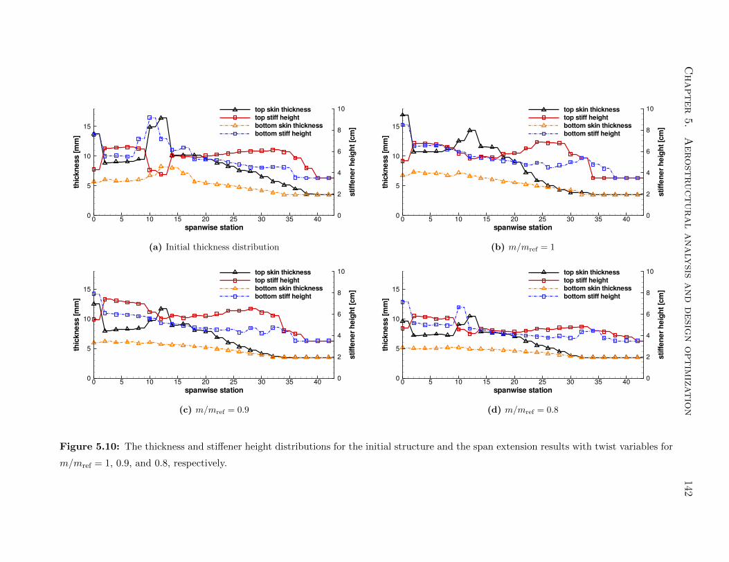
Chapter5.
Aerost
ructuralanaly
sisand
desig
noptim
ization
142
spanwise station
thickness[m
m]
stiffenerheight[cm]
0 5 10 15 20 25 30 35 400
5
10
15
0
2
4
6
8
10top skin thickness
top stiff height
bottom skin thickness
bottom stiff height
(a) Initial thickness distribution
spanwise station
thickness[m
m]
stiffenerheight[cm]
0 5 10 15 20 25 30 35 400
5
10
15
0
2
4
6
8
10top skin thickness
top stiff height
bottom skin thickness
bottom stiff height
(b) m/mref = 1
spanwise station
thickness[m
m]
stiffenerheight[cm]
0 5 10 15 20 25 30 35 400
5
10
15
0
2
4
6
8
10top skin thickness
top stiff height
bottom skin thickness
bottom stiff height
(c) m/mref = 0.9
spanwise stationthickness[m
m]
stiffenerheight[cm]
0 5 10 15 20 25 30 35 400
5
10
15
0
2
4
6
8
10top skin thickness
top stiff height
bottom skin thickness
bottom stiff height
(d) m/mref = 0.8
Figure 5.10: The thickness and stiffener height distributions for the initial structure and the span extension results with twist variables for
m/mref = 1, 0.9, and 0.8, respectively.
Chapter5.
Aerost
ructuralanaly
sisand
desig
noptim
ization
143
η
twist[degrees]
0 0.2 0.4 0.6 0.8 1
5
0
5
10
15jig
cruise
2.5g
1g
η
clc
0 0.2 0.4 0.6 0.8 1
2
0
2
4
6 cruise
2.5g
1g
(a) m/mref = 1
η
twist[degrees]
0 0.2 0.4 0.6 0.8 1
5
0
5
10
15jig
cruise
2.5g
1g
η
clc
0 0.2 0.4 0.6 0.8 1
2
0
2
4
6 cruise
2.5g
1g
(b) m/mref = 0.9
η
twist[degrees]
0 0.2 0.4 0.6 0.8 1
5
0
5
10
15jig
cruise
2.5g
1g
η
clc
0 0.2 0.4 0.6 0.8 1
2
0
2
4
6 cruise
2.5g
1g
(c) m/mref = 0.8
Figure 5.11: The twist and clc distributions for the span extension parametrization, for m/mref = 1, 0.9, and 0.8, respectively. Note that
these spans correspond to b/bref = 1.33, 1.20, and 0.993, respectively.
Chapter 6
Contributions, conclusions and future
work
In this chapter, I outline the main contributions from my thesis, summarize the main con-
clusions from each chapter and discuss future extensions of the work presented herein.
6.1 Contributions and conclusions
6.1.1 Homogenization-based beam theory
In Chapter 2, I presented a novel beam theory designed to accurately determine the through-
thickness stress and strain distribution in isotropic and composite beams. The proposed
beam theory includes several novel aspects, including the stress and strain representation
in the beam as a linear combination of the fundamental state solutions, and the use of ho-
mogenized stress, strain, and displacement quantities. This homogenization-based approach
enables a rigorous mathematical treatment with assumptions that can be tested against
three-dimensional solutions. The proposed beam theory contains a self-consistent proce-
dure to determine the shear strain correction matrix, and pressure corrections based on the
fundamental states. While some fundamental state solutions can be obtained for simple
geometries, it is difficult to obtain these solutions for realistic cross-sections with complex
geometries. To address this issue, I developed a finite-element approach to determine the fun-
damental state solutions for arbitrary cross-sections. I demonstrated that this approach can
be used to obtain highly accurate, three-dimensional stress and strain distributions in up to
three orders of magnitude less computational time when compared to full three-dimensional
calculations. The accuracy of the stress and strain distributions as well as the computational
144
Chapter 6. Contributions, conclusions and future work 145
efficiency, make this theory a powerful tool for analysis and design.
6.1.2 Structural analysis and design optimization
In Chapter 3, I presented a detailed description of the analysis of thin composite shell
structures. I presented high-order shell element formulations using both a displacement-
based approach and a mixed interpolation of tensorial component (MITC) formulation that
is not susceptible to shear and membrane locking [Dvorkin and Bathe, 1984, Bathe et al.,
2000]. Next, I presented parallel solution methods used to solve the large, sparse, linear
systems resulting from the finite-element discretization of thin shell structures. I outlined
the implementation of the direct Schur method and demonstrated its parallel scalability on
a series of extremely large finite-element problems. I demonstrated that the factorization
time for the direct Schur method is nearly independent of element order. I also discussed
the implementation of a new matrix ordering scheme, which I called AMD-OD. While ND
exhibited the most consistent parallel scalability, the AMD-OD scheme outperformed both
AMD and ND for the 24, 32 and 48 processor cases. Finally, I presented the sensitivity
analysis methods used to compute the derivatives of objectives of interest. The high-order
elements prove to be effective for analysis, yielding the most accurate solutions for a fixed
computational cost. On the other hand, the computational cost of computing the derivatives
of these higher-order elements increases dramatically with element order. Therefore, there
is a trade-off between accuracy of the solution and the computational cost of the gradients
for design problems.
6.1.3 Laminate parametrization
In Chapter 4, I presented a laminate parametrization technique for laminated composite
structures. This parametrization takes into account the discrete nature of the ply-angle vari-
ables that often arise due to manufacturing constraints. Frequently, these ply parametriza-
tion problems are solved with gradient-free approaches [Haftka and Walsh, 1992, Le Riche
and Haftka, 1993, Adams et al., 2004], however, this parametrization results in a continuous
formulation that is amenable to gradient-based design optimization. The parametrization
I developed, uses an exact penalty function to ensure that there are no intermediate plies
in the final design. I also present additional constraints that can be imposed to enforce
other manufacturing requirements such as a restriction on the number of contiguous plies
at the same angle [Haftka and Walsh, 1992], or that adjacent ply angles be restricted to a
reduced set of values. I demonstrated this ply parametrization on a series of problems: the
Chapter 6. Contributions, conclusions and future work 146
compliance minimization of a plate, the critical end-shortening maximization of a stiffened
panel, and a layup determination study of a composite wing.
6.1.4 Aerostructural analysis and design optimization
In Chapter 5, I presented an aerostructural optimization framework. This framework in-
cluded a consistent conservative load and displacement transfer scheme, a geometric parametriza-
tion based on free-form deformation volumes, an approximate Newton–Krylov solution al-
gorithm and a gradient-evaluation technique based on the adjoint method. I demonstrated
that an approximate Newton–Krylov method with periodic approximate Jacobian updates,
is fast, robust and exhibits good parallel scalability. In addition, I demonstrated that the
coupled adjoint system can be solved effectively using a Krylov subspace method. I applied
the aerostructural optimization framework to an aerostructural induced-drag minimization
study. I demonstrated the trade-offs between structural wing weight and induced drag. In
particular, the results show that it is possible to achieve a 43% induced drag reduction with
no weight penalty, a 28% induced drag reduction with a 10% wing weight reduction, or a
20% wing weight reduction with a 5% induced drag penalty from a baseline wing obtained
from a structural mass-minimization problem with fixed aerodynamic loads.
6.2 Future work
Dynamic analysis of beams The homogenization-based beam theory should be extended
to include dynamics. The extension to non-uniform through-thickness density distri-
butions would be particularly challenging, but may be important for the analysis of
sandwich structures.
Beam section design optimization The homogenization-based beam theory, in conjunc-
tion with the finite-element sectional analysis, provides a powerful tool for stress and
strain prediction. These analysis tools should be used to perform design optimization
of composite and isotropic cross-sections.
Extensions to curved beams The entire beam theory rests on the assumption that the
fundamental states are far-field solutions. Introducing curvature violates this assump-
tion. An extension of the beam theory to curved beams should be developed to account
for curvature, or to assess the errors in the analysis of curved beams.

Chapter 6. Contributions, conclusions and future work 147
Extension to nonlinear analysis The homogenization-based beam theory also relies on
the assumption that there are no material nonlinearities within the beam. For deep
beams, where large strains may occur, modeling material nonlinearity could be of
practical value.
Investigation of iso-geometric analysis for design The iso-geometric technique applied
to shell analysis has been a rapidly developing area of research [Hughes et al., 2005]. A
detailed assessment of the application of this analysis technique for structural design
optimization should be performed.
Simultaneous thickness and sequence design The laminate parametrization presented
in this thesis focused on laminate sequence design with a fixed-thickness distribution.
Better results could be obtained if the thickness-distribution and laminate sequence
design were performed simultaneously. The proposed laminate parametrization should
be extended to enable thickness changes.
Blended laminate designs The proposed laminate parametrization scheme should also
be extended to include a simultaneous sequence and blending design. In this combined
problem, the lamination sequence and the order of ply-additions and ply-removals could
be performed simultaneously.
Geometric parametrization While the free-form deformation approach presented in this
thesis was effective for the aerostructural optimization problems addressed herein, fur-
ther investigation of geometric parametrizations is warranted. In particular, the geo-
metric parametrization of the displaced shape should be considered, and methods for
moving the internal structure should be investigated.
Panel post-buckling analysis The analysis in this thesis has relied on a global-local ap-
proach to buckling analysis, where the local panels are examined for buckling using a
linearized buckling analysis with the local loads from a linear global analysis. These
local analyses should be extended to include possible post-buckling behaviour. This
will be important for the blended-wing-body (BWB) center fuselage sections where
large in-plane loads from wing bending, and pressure loads will act simultaneously.
The correct sizing of these structures will require post-buckling analysis and design.
Nonlinear structural kinematics Nonlinear structural kinematics should be used to ob-
tain the displaced shape of the wing. This will have important effects for large displace-
Chapter 6. Contributions, conclusions and future work 148
ments where a linear analysis will over-predict the displaced area due to the linearized
rotations.
Additional load conditions Additional load conditions must be considered within the
aerostructural design optimization framework to obtain realistic structural sizing re-
sults. These additional load cases include, but are not limited to, gust loads, landing
loads and inertial loads.
6.3 Epilogue
In the coming years, new aircraft designs will continue to employ increasing amounts of com-
posites and other advanced materials. Optimization techniques will play an ever-increasing
role in determining how best to use these materials. In this thesis I have endeavored to
develop tools and techniques that will facilitate the optimal usage of composite materials in
future aircraft. I have developed a novel beam theory to enable better analysis of thick com-
posite beams. I have examined parallel solution strategies for large finite-element problems
that may be used to better understand the behaviour of stresses in composite and isotropic
structures. I have developed a parametrization method that incorporates many manufac-
turing constraints that conventional methods do not include. Finally, in an integration of
these contributions, I have developed a parallel aerostructural analysis and optimization
framework that considers the multidisciplinary nature of aircraft design.

References
D. B. Adams, L. T. Watson, Z. Gurdal, and C. M. Anderson-Cook. Genetic algorithm optimizationand blending of composite laminates by locally reducing laminate thickness. Advances in Engi-neering Software, 35(1):35 – 43, 2004. ISSN 0965-9978. doi: 10.1016/j.advengsoft.2003.09.001.
S. Ahmad, B. M. Irons, and O. C. Zienkiewicz. Analysis of thick and thin shell structures by curvedfinite elements. International Journal for Numerical Methods in Engineering, 2:419–451, 1970.ISSN 1097-0207. doi: 10.1002/nme.1620020310.
G. Akhras, M. Cheung, and W. Li. Static and vibration analysis of anisotropic composite laminatesby finite strip method. International Journal of Solids and Structures, 30(22):3129 – 3137, 1993.ISSN 0020-7683. doi: 10.1016/0020-7683(93)90143-U.
C. Allen and T. Rendall. Unified approach to CFD-CSD interpolation and mesh motion using radialbasis functions. In 25th AIAA Applied Aerodynamics Conference, number 2007-3804, 2007.
P. R. Amestoy, T. A. Davis, and I. S. Duff. An approximate minimum degree ordering algorithm.SIAM Journal on Matrix Analysis and Applications, 17(4):886–905, 1996. ISSN 08954798. doi:10.1137/S0895479894278952.
P. R. Amestoy, I. S. Duff, and J. Y. L’Excellent. Multifrontal parallel distributed symmetric andunsymmetric solvers. Computer Methods in Applied Mechanics and Engineering, 184(2-4):501 –520, 2000. ISSN 0045-7825. doi: 10.1016/S0045-7825(99)00242-X.
C. Ashcraft and R. Grimes. SPOOLES: An object-oriented sparse matrix library. In Proceedingsof the 1999 SIAM Conference on Parallel Processing for Scientific Computing, March 1999.
I. Babuska and M. Suri. On locking and robustness in the finite element method. SIAM Journalon Numerical Analysis, 29(5):1261–1293, 1992. doi: 10.1137/0729075.
A. A. Baker, S. Dutton, and D. W. Kelly. Composite Materials for Aircraft Structures. AIAA Edu-cation Series. American Institute of Aeronautics and Astronautics, 2004. ISBN 9781563475405.
S. Balay, W. D. Gropp, L. C. McInnes, and B. F. Smith. Efficient management of parallelism inobject oriented numerical software libraries. In E. Arge, A. M. Bruaset, and H. P. Langtangen,editors, Modern Software Tools in Scientific Computing, pages 163–202. Birkhauser Press, 1997.
S. Balay, K. Buschelman, V. Eijkhout, W. D. Gropp, D. Kaushik, M. G. Knepley, L. C. McInnes,B. F. Smith, and H. Zhang. PETSc users manual. Technical Report ANL-95/11 - Revision 2.1.5,Argonne National Laboratory, 2004.
L. C. Bank. Shear coefficients for thin-walled composite beams. Composite Structures, 8(1):47 –61, 1987. ISSN 0263-8223. doi: 10.1016/0263-8223(87)90015-8.
149
REFERENCES 150
L. C. Bank and T. P. Melehan. Shear coefficients for multicelled thin-walled composite beams.Composite Structures, 11(4):259 – 276, 1989. ISSN 0263-8223. doi: 10.1016/0263-8223(89)90091-3.
M. Barcelos and K. Maute. Aeroelastic design optimization for laminar and turbulent flows. Com-puter Methods in Applied Mechanics and Engineering, 197(19-20):1813 – 1832, 2008. ISSN 0045-7825. doi: 10.1016/j.cma.2007.03.009.
M. Barcelos, H. Bavestrello, and K. Maute. A Schur-Newton-Krylov solver for steady-state aeroe-lastic analysis and design sensitivity analysis. Computer Methods in Applied Mechanics andEngineering, 195(17-18):2050 – 2069, 2006. ISSN 0045-7825. doi: 10.1016/j.cma.2004.09.013.
K.-J. Bathe. Finite element procedures. Prentice Hall, 2nd edition, 1996.
K.-J. Bathe and S. Bolourchi. A geometric and material nonlinear plate and shell element. Com-puters & Structures, 11(1-2):23 – 48, 1980. ISSN 0045-7949. doi: 10.1016/0045-7949(80)90144-3.
K.-J. Bathe and E. N. Dvorkin. A four-node plate bending element based on Mindlin/Reissner platetheory and a mixed interpolation. International Journal for Numerical Methods in Engineering,21:367–383, 1985. ISSN 1097-0207. doi: 10.1002/nme.1620210213.
K.-J. Bathe and E. N. Dvorkin. A formulation of general shell elements the use of mixed inter-polation of tensorial components. International Journal for Numerical Methods in Engineering,22:697–722, 1986. ISSN 1097-0207. doi: 10.1002/nme.1620220312.
K.-J. Bathe, A. Iosilevich, and D. Chapelle. An inf-sup test for shell finite elements. Computers &Structures, 75(5):439 – 456, 2000. ISSN 0045-7949. doi: 10.1016/S0045-7949(99)00213-8.
T. Belytschko, B. L. Wong, and H. Stolarski. Assumed strain stabilization procedure for the 9-node Lagrange shell element. International Journal for Numerical Methods in Engineering, 28(2):385–414, 1989. ISSN 1097-0207. doi: 10.1002/nme.1620280210.
V. L. Berdichevskii. Variational-asymptotic method of constructing a theory of shells. Journal ofApplied Mathematics and Mechanics, 43(4):711 – 736, 1979. ISSN 0021-8928. doi: 10.1016/0021-8928(79)90157-6.
G. Biros and O. Ghattas. Parallel Lagrange–Newton–Krylov–Schur methods for PDE-constrainedoptimization. Part I: The Krylov–Schur solver. SIAM Journal on Scientific Computing, 27(2):687–713, 2005a. doi: 10.1137/S106482750241565X.
G. Biros and O. Ghattas. Parallel Lagrange–Newton–Krylov–Schur methods for PDE-constrainedoptimization. Part II: The Lagrange–Newton solver and its application to optimal control ofsteady viscous flows. SIAM Journal on Scientific Computing, 27(2):714–739, 2005b. doi:10.1137/S1064827502415661.
T. Borrvall and J. Petersson. Topology optimization using regularized intermediate density control.Computer Methods in Applied Mechanics and Engineering, 190(3738):4911 – 4928, 2001. ISSN0045-7825. doi: 10.1016/S0045-7825(00)00356-X.
F. Brezzi and M. Fortin. Mixed and Hybrid Finite Element Methods. Springer-Verlag, 1991.
S. Brown. Displacement extrapolation for CFD+CSM aeroelastic analysis. AIAA Paper 97-1090,1997.
REFERENCES 151
M. Bruyneel. A general and effective approach for the optimal design of fiber reinforced compositestructures. Composites Science and Technology, 66(10):1303 – 1314, 2006. ISSN 0266-3538. doi:10.1016/j.compscitech.2005.10.011.
M. Bruyneel. SFP - A new parameterization based on shape functions for optimal material selection:application to conventional composite plies. Structural and Multidisciplinary Optimization, 43:17–27, 2011. ISSN 1615-147X. doi: 10.1007/s00158-010-0548-0.
M. Bruyneel and C. Fleury. Composite structures optimization using sequential convex program-ming. Advances in Engineering Software, 33(7-10):697 – 711, 2002. ISSN 0965-9978. doi:10.1016/S0965-9978(02)00053-4.
M. Bruyneel, P. Duysinx, C. Fleury, and T. Gao. Extensions of the shape functions with penaliza-tion parametrization for composite-ply optimization. AIAA Journal, 49(10):2325–2329, October2011. doi: 10.2514/1.J051225.
M. L. Bucalem and K.-J. Bathe. Higher-order MITC general shell elements. InternationalJournal for Numerical Methods in Engineering, 36:3729–3754, 1993. ISSN 1097-0207. doi:10.1002/nme.1620362109.
N. Buechter and E. Ramm. Shell theory versus degeneration a comparison in large rotation finiteelement analysis. International Journal for Numerical Methods in Engineering, 34:39–59, 1992.ISSN 1097-0207. doi: 10.1002/nme.1620340105.
E. Carrera. Historical review of zig-zag theories for multilayered plates and shells. Applied Me-chanics Reviews, 56(3):287–308, 2003. doi: 10.1115/1.1557614.
E. Carrera and G. Giunta. Refined beam theories based on a unified formulation. InternationalJournal of Applied Mechanics, 2:117–143, 2010. doi: 10.1142/S1758825110000500.
E. Carrera and M. Petrolo. On the effectiveness of higher-order terms in refined beam theories.Journal of Applied Mechanics, 78(2):021013, 2011. doi: 10.1115/1.4002207.
E. Carrera, G. Giunta, P. Nali, and M. Petrolo. Refined beam elements with arbitrary cross-section geometries. Computers & Structures, 88(5-6):283 – 293, 2010a. ISSN 0045-7949. doi:10.1016/j.compstruc.2009.11.002.
E. Carrera, G. Giunta, and M. Petrolo. Beam Structures: Classical and Advanced Theories. JohnWiley & Sons, 2010b. ISBN 978-0-470-97200-7.
E. Carrera, M. Petrolo, and P. Nali. Unified formulation applied to free vibrations finite ele-ment analysis of beams with arbitrary section. Shock and Vibration, 18(3):285–502, 2011. doi:10.3233/SAV-2010-0528.
C. E. S. Cesnik and D. H. Hodges. VABS: A new concept for composite rotor blade cross-sectionalmodeling. Journal of the American Helicopter Society, 42(1):27–38, 1997. ISSN 00028711. doi:10.4050/JAHS.42.27.
D. Chapelle and K.-J. Bathe. The Finite Element Analysis of Shells – Fundamentals. Springer,2003.
I. Chittick and J. R. R. A. Martins. Aero-structural optimization using adjoint coupled post-optimality sensitivities. Structural and Multidisciplinary Optimization, 36:59–70, 2008. ISSN1615-147X. doi: 10.1007/s00158-007-0200-9.
REFERENCES 152
I. Chittick and J. R. R. A. Martins. An asymmetric suboptimization approach to aerostructuraloptimization. Optimization and Engineering, 10(1):133–152, March 2009.
Z. Coulibaly and D. Orban. An `1 elastic interior-point method for mathematical programswith complementarity constraints. SIAM Journal on Optimization, 22(1):187–211, 2012. doi:10.1137/090777232.
G. Cowper. The shear coefficient in Timoshenko’s beam theory. Journal of Applied Mechanics, 33(5):335–340, 1966.
E. Cramer, J. Dennis, P. Frank, R. Lewis, and G. Shubin. Problem formulation for multidisciplinaryoptimization. SIAM Journal on Optimization, 4(4):754–776, 1994.
J. W. Demmel, S. C. Eisenstat, J. R. Gilbert, X. S. Li, and J. W. H. Liu. A supernodal approachto sparse partial pivoting. SIAM J. Matrix Analysis and Applications, 20(3):720–755, 1999.
S. Dharmarajan and H. McCutchen. Shear coefficients for orthotropic beams. Journal of CompositeMaterials, 7(4):530–535, 1973. doi: 10.1177/002199837300700411.
S. Dong, C. Alpdogan, and E. Taciroglu. Much ado about shear correction factors in Timoshenkobeam theory. International Journal of Solids and Structures, 47(13):1651 – 1665, 2010. ISSN0020-7683. doi: 10.1016/j.ijsolstr.2010.02.018.
S. B. Dong, J. B. Kosmatka, and H. C. Lin. On Saint–Venant’s problem for an inhomogeneous,anisotropic cylinder—Part I: Methodology for Saint–Venant solutions. Journal of Applied Me-chanics, 68(3):376–381, 2001. doi: 10.1115/1.1363598.
E. N. Dvorkin and K.-J. Bathe. A continuum mechanics based four-node shell element for generalnonlinear analysis. Engineering Computations, 1:77–88, 1984.
R. El Fatmi. Non-uniform warping including the effects of torsion and shear forces. Part I: A generalbeam theory. International Journal of Solids and Structures, 44(18-19):5912 – 5929, 2007a. ISSN0020-7683. doi: 10.1016/j.ijsolstr.2007.02.006.
R. El Fatmi. Non-uniform warping including the effects of torsion and shear forces. Part II: An-alytical and numerical applications. International Journal of Solids and Structures, 44(18-19):5930 – 5952, 2007b. ISSN 0020-7683. doi: 10.1016/j.ijsolstr.2007.02.005.
R. El Fatmi and H. Zenzri. On the structural behavior and the Saint–Venant solution in the exactbeam theory: Application to laminated composite beams. Computers & Structures, 80(16-17):1441 – 1456, 2002. ISSN 0045-7949. doi: 10.1016/S0045-7949(02)00090-1.
R. El Fatmi and H. Zenzri. A numerical method for the exact elastic beam theory. Applicationsto homogeneous and composite beams. International Journal of Solids and Structures, 41(9-10):2521 – 2537, 2004. ISSN 0020-7683. doi: 10.1016/j.ijsolstr.2003.12.011.
I. Elishakoff. Controversy associated with the so-called “follower forces”: Critical overview. AppliedMechanics Reviews, 58:117–142, 2005.
C. Farhat, M. Lesoinnea, and P. LeTallec. Load and motion transfer algorithms for fluid/structureinteraction problems with non–matching discrete interfaces: Momentum and energy conservation,optimal discretization and application to aeroelasticity. Computer methods in applied mechanicsand engineering, pages 95–115, 1996.
REFERENCES 153
C. A. Felippa, K. C. Park, and C. Farhat. Partitioned analysis of coupled mechanical systems.Computer Methods in Applied Mechanics and Engineering, 190(24-25):3247 – 3270, 2001. ISSN0045-7825. doi: 10.1016/S0045-7825(00)00391-1.
J. Foldager, J. S. Hansen, and N. Olhoff. A general approach forcing convexity of ply angleoptimization in composite laminates. Structural and Multidisciplinary Optimization, 16:201–211,1998. ISSN 1615-147X. doi: 10.1007/BF01202831.
H. Fukunaga and H. Sekine. Stiffness design method of symmetric laminates using laminationparameters. AIAA Journal, 30(11):2791–2793, 1992.
H. Fukunaga and G. N. Vanderplaats. Stiffness optimization of othrotropic laminated compositesusing lamination parameters. AIAA Journal, 29(4):641–646, 1991.
P. E. Gill, W. Murray, and M. A. Saunders. SNOPT: An SQP algorithm for large-scale constrainedoptimization. SIAM Review, 47(1):pp. 99–131, 2005. ISSN 00361445.
R. G. Grimes, J. G. Lewis, and H. D. Simon. A shifted block Lanczos algorithm for solving sparsesymmetric generalized eigenproblems. SIAM Journal on Matrix Analysis and Applications, 15(1):228–272, 1994. doi: 10.1137/S0895479888151111.
F. Gruttmann and W. Wagner. Shear correction factors in Timoshenko’s beam theory for arbi-trary shaped cross-sections. Computational Mechanics, 27:199–207, 2001. ISSN 0178-7675. doi:10.1007/s004660100239.
I. Guiamatsia. A new approach to plate theory based on through-thickness homogenization. Inter-national Journal for Numerical Methods in Engineering, 2010. doi: 10.1002/nme.2934.
I. Guiamatsia and J. S. Hansen. A homogenization-based laminated plate theory. ASME ConferenceProceedings, 2004(47004):421–436, 2004. doi: 10.1115/IMECE2004-61763.
R. Haftka and Z. Gurdal. Elements of Structural Optimization. Solid mechanics and its applications.Kluwer Academic Publishers, 1992. ISBN 9780792315049.
R. T. Haftka. Optimization of flexible wing structures subject to strength and induced drag con-straints. AIAA Journal, 15(8):1101–1106, August 1977.
R. T. Haftka and J. L. Walsh. Stacking-sequence optimization for buckling of laminated plates byinteger programming. AIAA Journal, 30(3):814–819, March 1992.
V. B. Hammer, M. P. Bendse, R. Lipton, and P. Pedersen. Parametrization in laminate design foroptimal compliance. International Journal of Solids and Structures, 34(4):415 – 434, 1997. ISSN0020-7683. doi: 10.1016/S0020-7683(96)00023-6.
J. S. Hansen and S. d. Almeida. A theory for laminated composite beams. Technical report,Instituto Tecnologico de Aeronautica, April 2001.
J. S. Hansen and G. R. Heppler. A Mindlin shell element that satisfies rigid-body requirements.AIAA Journal, 23(2):288–295, 1985. doi: 10.2514/3.8908.
J. S. Hansen, G. J. Kennedy, and S. F. M. de Almeida. A homogenization-based theory for laminatedand sandwich beams. In 7th International Conference on Sandwich Structures, pages 221–230,Aalborg University, Aalborg, Denmark, 2005.
REFERENCES 154
L. Hansen, W. Heinze, and P. Horst. Blended wing body structures in multidisciplinary pre-design. Structural and Multidisciplinary Optimization, 36:93–106, 2008. ISSN 1615-147X. doi:10.1007/s00158-007-0161-z.
M. Heil, A. Hazel, and J. Boyle. Solvers for large-displacement fluidstructure interaction problems:segregated versus monolithic approaches. Computational Mechanics, 43:91–101, 2008. ISSN0178-7675. doi: 10.1007/s00466-008-0270-6.
G. R. Heppler and J. S. Hansen. A Mindlin element for thick and deep shells. Computer methodsin applied mechanics and engineering, 54:21–47, 1986.
J. Hess and A. Smith. Calculation of potential flow about arbitrary bodies. Progress in AerospaceSciences, 8:1–138, 1967.
J. E. Hicken and D. W. Zingg. Parallel Newton–Krylov solver for the Euler equations discretizedusing simultaneous-approximation terms. AIAA Journal, 46:2773–2786, November 2008. doi:10.2514/1.34810.
J. E. Hicken and D. W. Zingg. A simplified and flexible variant of GCROT for solving nonsym-metric linear systems. SIAM Journal on Scientific Computing, 32(3):1672–1694, 2010a. doi:10.1137/090754674.
J. E. Hicken and D. W. Zingg. Induced drag minimization of nonplanar geometries based on theEuler equations. AIAA Journal, 48(11):2564–2575, November 2010b. doi: 10.2514/1.J050379.
G. Horrigmoe and P. G. Bergan. Nonlinear analysis of free-form shells by flat finite elements.Computer Methods in Applied Mechanics and Engineering, 16(1):11 – 35, 1978. ISSN 0045-7825.doi: 10.1016/0045-7825(78)90030-0.
P. C. Hughes. Spacecraft attitude dynamics. Dover books on engineering. Dover Publications, 2004.ISBN 9780486439259.
T. Hughes, J. Cottrell, and Y. Bazilevs. Isogeometric analysis: CAD, finite elements, NURBS, exactgeometry and mesh refinement. Computer Methods in Applied Mechanics and Engineering, 194(39-41):4135 – 4195, 2005. ISSN 0045-7825. doi: 10.1016/j.cma.2004.10.008.
T. J. R. Hughes and F. Brezzi. On drilling degrees of freedom. Computer Methods in AppliedMechanics and Engineering, 72:105–121, 1989.
T. J. R. Hughes and W. K. Liu. Nonlinear finite element analysis of shells: Part I. Three-dimensionalshells. Computer Methods in Applied Mechanics and Engineering, 26(3):331 – 362, 1981. ISSN0045-7825. doi: 10.1016/0045-7825(81)90121-3.
T. J. R. Hughes, R. L. Taylor, and W. Kanoknukulchai. A simple and efficient finite element forplate bending. International Journal for Numerical Methods in Engineering, 11:1529–1543, 1977.ISSN 1097-0207. doi: 10.1002/nme.1620111005.
T. J. R. Hughes, M. Cohen, and M. Haroun. Reduced and selective integration techniques in thefinite element analysis of plates. Nuclear Engineering and Design, 46(1):203 – 222, 1978. ISSN0029-5493. doi: 10.1016/0029-5493(78)90184-X. Special Issue Structural Mechanics in ReactorTechnology-Smirt-4.
REFERENCES 155
J. R. Hutchinson. Shear coefficients for Timoshenko beam theory. Journal of Applied Mechanics,68(1):87–92, 2001. doi: 10.1115/1.1349417.
C. Hvejsel, E. Lund, and M. Stolpe. Optimization strategies for discrete multi-material stiffnessoptimization. Structural and Multidisciplinary Optimization, 44:149–163, 2011. ISSN 1615-147X.doi: 10.1007/s00158-011-0648-5.
D. Iesan. On Saint–Venant’s problem. Archive for Rational Mechanics and Analysis, 91:363–373,1986a. ISSN 0003-9527. doi: 10.1007/BF00282340.
D. Iesan. On the theory of uniformly loaded cylinders. Journal of Elasticity, 16:375–382, 1986b.ISSN 0374-3535. doi: 10.1007/BF00041762.
S. T. IJsselmuiden, M. M. Abdalla, and Z. Gurdal. Implementation of strength-based failurecriteria in the lamination parameter design space. AIAA Journal, 46(7):1826–1834, July 2008.doi: 10.2514/1.35565.
K. A. James, J. S. Hansen, and J. R. R. A. Martins. Structural topology optimization for multipleload cases while avoiding local minima. April 2008. AIAA 2008-2287.
K. A. James, J. S. Hansen, and J. R. R. A. Martins. Structural topology optimization for multipleload cases using a dynamic aggregation technique. Engineering Optimization, 41(12):1103–1118,December 2009. doi: 10.1080/03052150902926827.
P. Jansen, R. E. Perez, and J. R. R. A. Martins. Aerostructural optimization of nonplanar liftingsurfaces. Journal of Aircraft, 47(5):1491–1503, 2010. doi: 10.2514/1.44727.
D. C. Jegley, A. Velicki, and D. A. Hansen. Structural efficiency of stitched rod-stiffened com-posite panels with stiffener crippling. In 43rd AIAA/ASME/ASCE/AHS Structures, StructuralDynamics and Materials Conference, Denver CO, United States, number 2002-1728, 2002.
R. M. Jones. Mechanics of Composite Materials. Technomic Publishing Co., 1996.
R. T. Jones. The spanwise distribution of lift for minimum induced drag of wings having a givenlift and a given bending moment. Technical Report TN-2249, NASA, December 1950.
R. T. Jones and T. A. Lasinski. Effect of winglets on the induced drag of ideal wing shapes.Technical Report TM-81230, NASA, September 1980.
G. Karypis and V. Kumar. A fast and high quality multilevel scheme for partitioning irregulargraphs. SIAM Journal on Scientific Computing, 20(1):359–392, 1998.
J. Katz and A. Plotkin. Low–Speed Aerodynamics. McGraw–Hill Inc., 1991.
G. J. Kennedy and J. R. R. A. Martins. Parallel solution methods for aerostructural analysisand design optimization. In Proceedings of the 13th AIAA/ISSMO Multidisciplinary AnalysisOptimization Conference, Fort Worth, TX, September 2010. AIAA 2010-9308.
G. J. Kennedy and J. R. R. A. Martins. A homogenization-based theory for anisotropic beamswith accurate through-section stress and strain prediction. International Journal of Solids andStructures, 2011. doi: 10.1016/j.ijsolstr.2011.09.012.

REFERENCES 156
G. J. Kennedy and J. R. R. A. Martins. A regularized discrete laminate parametrization techniquewith applications to wing-box design optimization. In 53rd AIAA/ASME/ASCE/AHS/ASCStructures, Structural Dynamics, and Materials Conference, Honolulu, HI, April 2012. AIAA-2012-1519.
G. J. Kennedy, J. R. R. A. Martins, and J. S. Hansen. Aerostructural optimization of aircraftstructures using asymmetric subspace optimization. In 12th AIAA/ISSMO MultidisciplinaryAnalysis and Optimization Conference, Victoria, BC. AIAA, 2008. AIAA-2008-5847.
G. J. Kennedy, J. S. Hansen, and J. R. R. A. Martins. A Timoshenko beam theory with pressurecorrections for layered orthotropic beams. International Journal of Solids and Structures, 48(16-17):2373 – 2382, 2011. ISSN 0020-7683. doi: 10.1016/j.ijsolstr.2011.04.009.
G. K. W. Kenway, G. J. Kennedy, and J. R. R. A. Martins. A scalable parallel approach forhigh-fidelity aerostructural analysis and optimization. In 53rd AIAA/ASME/ASCE/AHS/ASCStructures, Structural Dynamics, and Materials Conference, Honolulu, HI, April 2012. AIAA-2012-1922.
J. Kim, N. Aluru, and D. Tortorelli. Improved multi-level Newton solvers for fully coupled multi-physics problems. International Journal for Numerical Methods in Engineering, 58:463–480,2003. ISSN 1097-0207. doi: 10.1002/nme.751.
D. Knoll and D. Keyes. Jacobian–free Newton-Krylov methods: a survey of approaches and appli-cations. Journal of Computational Physics, 193(2):357–397, 2004.
J. B. Kosmatka, H. C. Lin, and S. B. Dong. On Saint–Venant’s problem for an inhomogeneous,anisotropic cylinder—Part II: Cross-sectional properties. Journal of Applied Mechanics, 68(3):382–391, 2001. doi: 10.1115/1.1365152.
I. M. Kroo. Drag due to lift: Concepts for prediction and reduction. Annual Review of FluidMechanics, 33:587–617, November 2000.
P. Ladeveze and J. Simmonds. New concepts for linear beam theory with arbitrary geometry andloading. European Journal of Mechanics - A/Solids, 17(3):377 – 402, 1998. ISSN 0997-7538. doi:10.1016/S0997-7538(98)80051-X.
P. Ladeveze, P. Sanchez, and J. G. Simmonds. On application of the exact theory of elasticbeams. In D. Durban, D. Givoli, J. G. Simmonds, and G. M. L. Gladwell, editors, Advances inthe Mechanics of Plates and Shells, volume 88 of Solid Mechanics and Its Applications, pages181–196. Springer Netherlands, 2002. ISBN 978-0-306-46954-1. doi: 10.1007/0-306-46954-5-12.
C. L. Lawson, R. J. Hanson, D. R. Kincaid, and F. T. Krogh. Basic linear algebra subprogramsfor fortran usage. ACM Trans. Math. Softw., 5:308–323, September 1979. ISSN 0098-3500. doi:10.1145/355841.355847.
R. Le Riche and R. T. Haftka. Optimization of laminate stacking sequence for buckling loadmaximization by genetic algorithm. AIAA Journal, 31(5):951–956, May 1993.
S. Lekhnitskii. Strength calculation of composite beams. Vestnik inzhen i tekhnikov, (9), 1935.
V. Li and A. Velicki. Advanced PRSEUS structural concept design and optimization. In 12thAIAA/ISSMO Multidisciplinary Analysis and Optimization Conference, Victoria BC, Canada,number 2008-5840, 2008.
REFERENCES 157
X. S. Li and J. W. Demmel. SuperLU DIST: A scalable distributed-memory sparse direct solverfor unsymmetric linear systems. ACM Trans. Mathematical Software, 29(2):110–140, June 2003.
L. Librescu and O. Song. Thin-walled composite beams: Theory and application. Solid mechanicsand its applications. Springer, 2006. ISBN 9781402034572.
R. H. Liebeck. Design of the blended wing body subsonic transport. Journal of Aircraft, 41(1):10–25, 2004. doi: 10.2514/1.9084.
B. Liu and R. T. Haftka. Single-level composite wing optimization based on flexural laminationparameters. Structural and Multidisciplinary Optimization, 26:111–120, 2004. ISSN 1615-147X.doi: 10.1007/s00158-003-0315-6.
B. Liu, R. T. Haftka, and M. A. Akgun. Two-level composite wing structural optimization usingresponse surfaces. Structural and Multidisciplinary Optimization, 20:87–96, 2000a. ISSN 1615-147X. doi: 10.1007/s001580050140.
B. Liu, R. T. Haftka, M. A. Akgn, and A. Todoroki. Permutation genetic algorithm for stacking se-quence design of composite laminates. Computer Methods in Applied Mechanics and Engineering,186(24):357 – 372, 2000b. ISSN 0045-7825. doi: 10.1016/S0045-7825(99)90391-2.
B. Liu, R. T. Haftka, and P. Trompette. Maximization of buckling loads of composite panels usingflexural lamination parameters. Structural and Multidisciplinary Optimization, 26:28–36, 2004.ISSN 1615-147X. doi: 10.1007/s00158-003-0314-7.
K. H. Lo, R. M. Christensen, and E. M. Wu. A high-order theory of plate deformation—part 1: Ho-mogeneous plates. Journal of Applied Mechanics, 44(4):663–668, 1977a. doi: 10.1115/1.3424154.
K. H. Lo, R. M. Christensen, and E. M. Wu. A high-order theory of plate deformation—part 2:Laminated plates. Journal of Applied Mechanics, 44(4):669–676, 1977b. doi: 10.1115/1.3424155.
C. Loken, D. Gruner, L. Groer, R. Peltier, N. Bunn, M. Craig, T. Henriques, J. Dempsey, C.-H.Yu, J. Chen, L. J. Dursi, J. Chong, S. Northrup, J. Pinto, N. Knecht, and R. V. Zon. SciNet:Lessons learned from building a power-efficient top-20 system and data centre. Journal of Physics:Conference Series, 256(1):012026, 2010.
A. E. H. Love. A Treatise on the Mathematical Theory of Elasticity. Cambridge University Press,3rd edition, 1920.
E. Lund. Buckling topology optimization of laminated multi-material composite shellstructures. Composite Structures, 91(2):158 – 167, 2009. ISSN 0263-8223. doi:10.1016/j.compstruct.2009.04.046.
R. H. MacNeal and R. L. Harder. A proposed standard set of problems to test finite elementaccuracy. Finite Elements in Analysis and Design, 1:3–20, 1985.
N. Maman and C. Farhat. Matching fluid and structure meshes for aeroelastic computations: aparallel approach. Computers and Structures, 54(4):779–785, 1995.
J. R. R. A. Martins and A. B. Lambe. Multidisciplinary design optimization: Survey of architec-tures. AIAA Journal, 2012. Submitted.
J. R. R. A. Martins, P. Sturdza, and J. J. Alonso. The complex-step derivative approximation. ACMTransactions on Mathematical Software, 29(3):245–262, Sept. 2003. doi: 10.1145/838250.838251.
REFERENCES 158
J. R. R. A. Martins, J. J. Alonso, and J. J. Reuther. High-fidelity aerostructural design optimizationof a supersonic business jet. Journal of Aircraft, 41(3):523–530, 2004. doi: 10.2514/1.11478.
J. R. R. A. Martins, J. J. Alonso, and J. J. Reuther. A coupled–adjoint sensitivity analysis methodfor high–fidelity aero–structural design. Optimization and Engineering, 6:33–62, 2005. doi:10.1023/B:OPTE.0000048536.47956.62.
W. Mason and L. Herrmann. Elastic shear analysis of general prismatic beams. Journal EngineeringMechanics Division ASCE, 94:965–983, 1968.
K. Maute and M. Allen. Conceptual design of aeroelastic structures by topology optimization.Structural and Multidisciplinary Optimization, 27:27–42, 2004.
K. Maute, M. Nikbay, and C. Farhat. Coupled analytical sensitivity analysis and optimization ofthree-dimensional nonlinear aeroelastic systems. AIAA Journal, 39(11):2051–2061, 2001.
M. Miki and Y. Sugiyama. Optimum design of laminated composites plates using laminationparameters. AIAA Journal, 31(5):921–922, 1993.
R. V. Milford and W. C. Schnobrich. Degenerated isoparametric finite elements using explicitintegration. International Journal for Numerical Methods in Engineering, 23:133–154, 1986.ISSN 1097-0207. doi: 10.1002/nme.1620230111.
S. A. Ning and I. Kroo. Multidisciplinary considerations in the design of wings and wing tip devices.Journal of Aircraft, 47(2):534–543, 2010. doi: 10.2514/1.41833.
J. Nocedal and S. J. Wright. Numerical Optimization. Springer, 1999.
N. J. Pagano and R. B. Pipes. The influence of stacking sequence on laminate strength. Journalof Composite Materials, 5(1):50–57, 1971.
H. Parisch. Geometrical nonlinear analysis of shells. Computer Methods in Applied Mechanics andEngineering, 14(2):159 – 178, 1978. ISSN 0045-7825. doi: 10.1016/0045-7825(78)90091-9.
R. E. Perez, P. W. Jansen, and J. R. R. A. Martins. pyOpt: a Python-based object-orientedframework for nonlinear constrained optimization. Structural and Multidisciplinary Optimization,45(1):101–118, 2012. doi: 10.1007/s00158-011-0666-3.
R. B. Pipes and N. Pagano. Interlaminar stresses in composite laminates under uniform axial ex-tension. Journal of Composite Materials, 4(4):538–548, 1970. doi: 10.1177/002199837000400409.
R. J. Plank and W. H. Wittrick. Buckling under combined loading of thin, flat-walled structuresby a complex finite strip method. International Journal for Numerical Methods in Engineering,8(2):323–339, 1974. ISSN 1097-0207. doi: 10.1002/nme.1620080211.
N. Poon and J. R. R. A. Martins. An adaptive approach to constraint aggregation using adjointsensitivity analysis. Structural and Multidisciplinary Optimization, 34:61–73, 2007. ISSN 1615-147X. doi: 10.1007/s00158-006-0061-7.
B. Popescu and D. H. Hodges. On asymptotically correct Timoshenko-like anisotropic beam theory.International Journal of Solids and Structures, 37(3):535 – 558, 2000. ISSN 0020-7683. doi:10.1016/S0020-7683(99)00020-7.
REFERENCES 159
J. Prescott. Elastic waves and vibrations of thin rods. Philosophical Magazine, 33:703–754, 1942.doi: 10.1080/14786444208521261.
J. N. Reddy. A generalization of two-dimensional theories of laminated composite plates.Communications in Applied Numerical Methods, 3(3):173–180, 1987. ISSN 1555-2047. doi:10.1002/cnm.1630030303.
T. Rendall and C. Allen. Unified fluid–structure interpolation and mesh motion using radial basisfunctions. International journal for numerical methods in engineering, 74:1519–1559, 2008.
J. J. Reuther, J. J. Alonso, J. R. R. A. Martins, and S. C. Smith. A coupled aero-structuraloptimization method for complete aircraft configurations. AIAA paper 99-0187, 1999.
Y. Saad. Numerical methods for large eigenvalue problems. Algorithms and architectures foradvanced scientific computing. Manchester University Press, 1992. ISBN 9780719033865.
Y. Saad. A fexible inner-outer preconditioned GMRES algorithm. SIAM Journal on ScientificComputing, 14(2):461–469, 1993. doi: 10.1137/0914028.
Y. Saad. Iterative Methods for Sparse Linear Systems. PWS Pub. Co., 2nd edition, 2003.
Y. Saad and M. H. Schultz. GMRES: A generalized minimal residual algorithm for solving non-symmetric linear systems. SIAM Journal on Scientific and Statistical Computing, 7(3):856–869,1986. doi: 10.1137/0907058.
Y. Saad and M. Sosonikina. Distributed Schur complement techniques for general sparse linearsystems. SIAM Journal of Scientific Computing, 21(4):1337–1356, 1999.
H. Scheel and S. Scholtes. Mathematical programs with complementarity constraints: Stationarity,optimality, and sensitivity. Mathematics of Operations Research, 25(1):pp. 1–22, 2000. ISSN0364765X.
S. Scholtes. Convergence properties of a regularization scheme for mathematical programs with com-plementarity constraints. SIAM Journal on Optimization, 11(4):918–936, 2001. ISSN 10526234.doi: 10.1137/S1052623499361233.
U. Schramm, L. Kitis, W. Kang, and W. D. Pilkey. On the shear deformation coefficient in beamtheory. Finite Elements in Analysis and Design, 16(2):141 – 162, 1994. ISSN 0168-874X. doi:10.1016/0168-874X(94)00008-5.
T. W. Sederberg and S. R. Parry. Free-form deformation of solid geometric mod-els. SIGGRAPH Comput. Graph., 20(4):151–160, 1986. ISSN 0097-8930. doi:http://doi.acm.org/10.1145/15886.15903.
A. P. Seyranian, E. Lund, and N. Olhoff. Multiple eigenvalues in structural optimization prob-lems. Structural and Multidisciplinary Optimization, 8:207–227, 1994. ISSN 1615-147X. doi:10.1007/BF01742705.
O. Sigmund and S. Torquato. Design of materials with extreme thermal expansion using a three-phase topology optimization method. Journal of the Mechanics and Physics of Solids, 45(6):1037 – 1067, 1997. ISSN 0022-5096. doi: 10.1016/S0022-5096(96)00114-7.
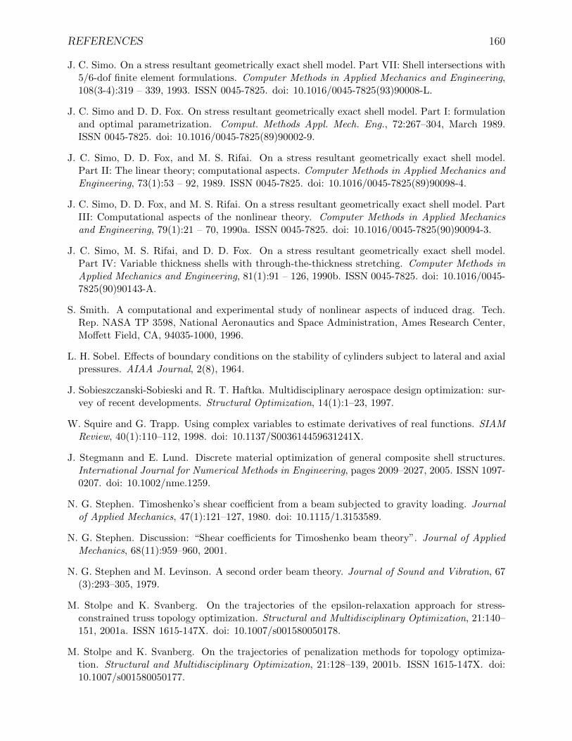
REFERENCES 160
J. C. Simo. On a stress resultant geometrically exact shell model. Part VII: Shell intersections with5/6-dof finite element formulations. Computer Methods in Applied Mechanics and Engineering,108(3-4):319 – 339, 1993. ISSN 0045-7825. doi: 10.1016/0045-7825(93)90008-L.
J. C. Simo and D. D. Fox. On stress resultant geometrically exact shell model. Part I: formulationand optimal parametrization. Comput. Methods Appl. Mech. Eng., 72:267–304, March 1989.ISSN 0045-7825. doi: 10.1016/0045-7825(89)90002-9.
J. C. Simo, D. D. Fox, and M. S. Rifai. On a stress resultant geometrically exact shell model.Part II: The linear theory; computational aspects. Computer Methods in Applied Mechanics andEngineering, 73(1):53 – 92, 1989. ISSN 0045-7825. doi: 10.1016/0045-7825(89)90098-4.
J. C. Simo, D. D. Fox, and M. S. Rifai. On a stress resultant geometrically exact shell model. PartIII: Computational aspects of the nonlinear theory. Computer Methods in Applied Mechanicsand Engineering, 79(1):21 – 70, 1990a. ISSN 0045-7825. doi: 10.1016/0045-7825(90)90094-3.
J. C. Simo, M. S. Rifai, and D. D. Fox. On a stress resultant geometrically exact shell model.Part IV: Variable thickness shells with through-the-thickness stretching. Computer Methods inApplied Mechanics and Engineering, 81(1):91 – 126, 1990b. ISSN 0045-7825. doi: 10.1016/0045-7825(90)90143-A.
S. Smith. A computational and experimental study of nonlinear aspects of induced drag. Tech.Rep. NASA TP 3598, National Aeronautics and Space Administration, Ames Research Center,Moffett Field, CA, 94035-1000, 1996.
L. H. Sobel. Effects of boundary conditions on the stability of cylinders subject to lateral and axialpressures. AIAA Journal, 2(8), 1964.
J. Sobieszczanski-Sobieski and R. T. Haftka. Multidisciplinary aerospace design optimization: sur-vey of recent developments. Structural Optimization, 14(1):1–23, 1997.
W. Squire and G. Trapp. Using complex variables to estimate derivatives of real functions. SIAMReview, 40(1):110–112, 1998. doi: 10.1137/S003614459631241X.
J. Stegmann and E. Lund. Discrete material optimization of general composite shell structures.International Journal for Numerical Methods in Engineering, pages 2009–2027, 2005. ISSN 1097-0207. doi: 10.1002/nme.1259.
N. G. Stephen. Timoshenko’s shear coefficient from a beam subjected to gravity loading. Journalof Applied Mechanics, 47(1):121–127, 1980. doi: 10.1115/1.3153589.
N. G. Stephen. Discussion: “Shear coefficients for Timoshenko beam theory”. Journal of AppliedMechanics, 68(11):959–960, 2001.
N. G. Stephen and M. Levinson. A second order beam theory. Journal of Sound and Vibration, 67(3):293–305, 1979.
M. Stolpe and K. Svanberg. On the trajectories of the epsilon-relaxation approach for stress-constrained truss topology optimization. Structural and Multidisciplinary Optimization, 21:140–151, 2001a. ISSN 1615-147X. doi: 10.1007/s001580050178.
M. Stolpe and K. Svanberg. On the trajectories of penalization methods for topology optimiza-tion. Structural and Multidisciplinary Optimization, 21:128–139, 2001b. ISSN 1615-147X. doi:10.1007/s001580050177.
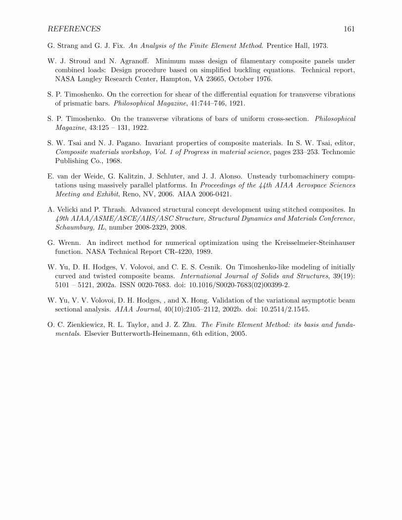
REFERENCES 161
G. Strang and G. J. Fix. An Analysis of the Finite Element Method. Prentice Hall, 1973.
W. J. Stroud and N. Agranoff. Minimum mass design of filamentary composite panels undercombined loads: Design procedure based on simplified buckling equations. Technical report,NASA Langley Research Center, Hampton, VA 23665, October 1976.
S. P. Timoshenko. On the correction for shear of the differential equation for transverse vibrationsof prismatic bars. Philosophical Magazine, 41:744–746, 1921.
S. P. Timoshenko. On the transverse vibrations of bars of uniform cross-section. PhilosophicalMagazine, 43:125 – 131, 1922.
S. W. Tsai and N. J. Pagano. Invariant properties of composite materials. In S. W. Tsai, editor,Composite materials workshop, Vol. 1 of Progress in material science, pages 233–253. TechnomicPublishing Co., 1968.
E. van der Weide, G. Kalitzin, J. Schluter, and J. J. Alonso. Unsteady turbomachinery compu-tations using massively parallel platforms. In Proceedings of the 44th AIAA Aerospace SciencesMeeting and Exhibit, Reno, NV, 2006. AIAA 2006-0421.
A. Velicki and P. Thrash. Advanced structural concept development using stitched composites. In49th AIAA/ASME/ASCE/AHS/ASC Structure, Structural Dynamics and Materials Conference,Schaumburg, IL, number 2008-2329, 2008.
G. Wrenn. An indirect method for numerical optimization using the Kreisselmeier-Steinhauserfunction. NASA Technical Report CR-4220, 1989.
W. Yu, D. H. Hodges, V. Volovoi, and C. E. S. Cesnik. On Timoshenko-like modeling of initiallycurved and twisted composite beams. International Journal of Solids and Structures, 39(19):5101 – 5121, 2002a. ISSN 0020-7683. doi: 10.1016/S0020-7683(02)00399-2.
W. Yu, V. V. Volovoi, D. H. Hodges, , and X. Hong. Validation of the variational asymptotic beamsectional analysis. AIAA Journal, 40(10):2105–2112, 2002b. doi: 10.2514/2.1545.
O. C. Zienkiewicz, R. L. Taylor, and J. Z. Zhu. The Finite Element Method: its basis and funda-mentals. Elsevier Butterworth-Heinemann, 6th edition, 2005.
Appendix A
Shell element tests
In this appendix, I present a series of examples of the displacement-based and MITC-based
shell element formulations presented in Section 3.1. Figure A.1 and Figure A.2 show accu-
racy studies for the displacement and MITC-based shell elements for a fully clamped plate
subject to a uniform pressure load, and a cylinder subject to a sinusoidally varying pressure
distribution, p(x, θ) = p0 sin(x/L) sin(θ), respectively. In both test cases, the computations
are performed on distorted finite-element meshes that are not aligned with the coordinate
lines of the natural shell parametrizations. These distorted meshes make for a more diffi-
cult accuracy test. The MITC-based shell elements of all orders perform better than their
displacement-based counterparts. In particular, the low-order MITC shell elements exhibit
far better behaviour than the low-order displacement-based elements.
Figure A.3a shows a comparison of the prediction of the snap-through behaviour of a
partial cylinder subject to a central point load. Note that Horrigmoe and Bergan [1978]
used a coarse mesh due to the limited memory available on computers at the time. I have
run results with the original mesh and a mesh with nine-times as many degrees of freedom
with 4th order MITC shell elements. The original and more refined snap-through behaviour
exhibit similar trends, with the more-refined mesh predicting a smaller snap-through load.
Figure A.3b shows a comparison of the critical pressure loads obtained from the 4th order
MITC shell elements and those calculations performed by Sobel [1964] using the Donnell
equations. The relative difference between the two predictions is also plotted in Figure A.3b.
These results demonstrate that the discrepancy between the two models is between 2% and
4%.
162
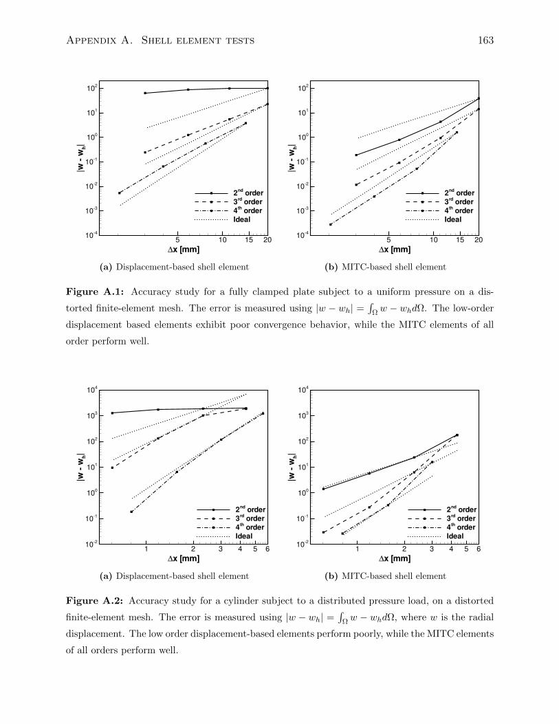
Appendix A. Shell element tests 163
∆x [mm]
|ww
h|
5 10 15 2010
4
103
102
101
100
101
102
2ndorder
3rdorder
4thorder
Ideal
(a) Displacement-based shell element
∆x [mm]
|ww
h|
5 10 15 2010
4
103
102
101
100
101
102
2ndorder
3rdorder
4thorder
Ideal
(b) MITC-based shell element
Figure A.1: Accuracy study for a fully clamped plate subject to a uniform pressure on a dis-
torted finite-element mesh. The error is measured using |w − wh| =∫
Ωw − whdΩ. The low-order
displacement based elements exhibit poor convergence behavior, while the MITC elements of all
order perform well.
∆x [mm]
|ww
h|
1 2 3 4 5 610
2
101
100
101
102
103
104
2ndorder
3rdorder
4thorder
Ideal
(a) Displacement-based shell element
∆x [mm]
|ww
h|
1 2 3 4 5 610
2
101
100
101
102
103
104
2ndorder
3rdorder
4thorder
Ideal
(b) MITC-based shell element
Figure A.2: Accuracy study for a cylinder subject to a distributed pressure load, on a distorted
finite-element mesh. The error is measured using |w − wh| =∫
Ωw − whdΩ, where w is the radial
displacement. The low order displacement-based elements perform poorly, while the MITC elements
of all orders perform well.
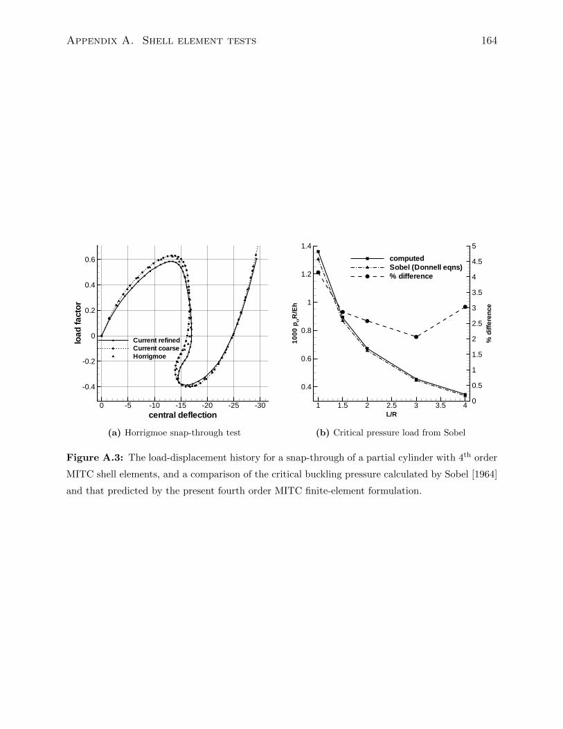
Appendix A. Shell element tests 164
central deflection
load
fact
or
-30-25-20-15-10-50
-0.4
-0.2
0
0.2
0.4
0.6
Current refinedCurrent coarseHorrigmoe
(a) Horrigmoe snap-through test
L/R
1000
p crR
/Eh
%di
ffer
ence
1 1.5 2 2.5 3 3.5 4
0.4
0.6
0.8
1
1.2
1.4
0
0.5
1
1.5
2
2.5
3
3.5
4
4.5
5
computedSobel (Donnell eqns)% difference
(b) Critical pressure load from Sobel
Figure A.3: The load-displacement history for a snap-through of a partial cylinder with 4th order
MITC shell elements, and a comparison of the critical buckling pressure calculated by Sobel [1964]
and that predicted by the present fourth order MITC finite-element formulation.


![A parallel aerostructural optimization framework for ...gkennedy.gatech.edu/wp-content/uploads/2014/12/... · Kenway et al.[2014] developed a more scalable coupled adjoint for high-fidelity](https://img.pdfslide.us/doc/110x75/60861d0cf4cbbc490c47d545/a-parallel-aerostructural-optimization-framework-for-kenway-et-al2014-developed.jpg)