Aero-Optics of Supersonic Boundary Layers

49th AIAA Aerospace Sciences Meeting and Exhibit AIAA-2011-1325 4-7 January 2011, Orlando, FL

American Institute of Aeronautics and Astronautics

Aero-Optics of Supersonic Boundary Layers.

Stanislav Gordeyev*, Eric Jumper†

Department of Aerospace and Mechanical Engineering, ,

University of Notre Dame, Notre Dame, IN 46556

and

Tim E. Hayden‡

Department of Aeronautics,

US Air Force Academy, Colorado Springs. , CO 80840

Aero-optical measurements of a zero-pressure-gradient, supersonic boundary layer along the test section wall at M=2.0 were performed using a Malley probe. The Malley probe captured both the amplitude of optical distortions and the convective speed. The convective speed of the optically-active structures inside the supersonic boundary layer was found to be 0.84 of the freestream speed. The deflection-angle spectra were found to collapse with the local displacement thickness. The streamwise correlation function for the supersonic boundary layer revealed the presence of a pseudo-periodic structure with the typical size of 1.5 of the local boundary-layer thickness. A new model was developed to describe aero-optical effects of both the subsonic and the supersonic boundary layers. Finally, this new model and several other theoretical scalings were tested in the attempt to collapse both subsonic and supersonic boundary layer aero-optical results.

I. Background ASER-based free-space communication systems offer high transmission rates through the atmosphere, on the order of Terabytes per second. Once link is established, high-speed, secure communication link between a

ground stations, aircrafts or satellites becomes possible; however, when the link involves aircraft, turbulent flow around the aircraft introduces density fluctuations, which can distort the emerging laser beam and significantly reduce laser intensity on a target [1,2]. These aero-optical effects increase significantly with Mach number and may force the airborne free-space communication systems to be inoperable at transonic and supersonic speeds. Large-scale vortical structures inside shear layers and wakes behind bluff bodies introduce significant turbulent fluctuations and can impose large aero-optical distortions on the laser beam even at moderate subsonic speeds [3,4]. Attached turbulent boundary layers, while producing less density fluctuations compared to shear layers and wakes, have also shown to potentially create significant aero-optical distortions at high transonic and supersonic speeds [5,6]. Aero-optical distortions produced by subsonic boundary layers were extensively experimentally studied in the last forty years [3,5-8]. Supersonic and hypersonic boundary layers, on the other hand, have been given significantly less-attention, partially because of experimental difficulties in making reliable optical measurements at high speeds. Stine and Winovich [9] in 1956 experimentally investigated the optical transmission characteristics of compressible turbulent boundary layers for Mach number range from 0.4 to 2.5 by measuring the time-average intensity of light for flow-on cases compared to a flow-off case. They compared their experimental finding to the theoretical predictions of Liepmann [10] and found reasonably-good agreement. Later these experimental results were further analyzed by Sutton [11], where he calculated length scales and provided simple scaling for optical MTF (Modulation Transfer Function) to compute the level of optical degradation caused by compressible boundary layers for different flight regimes. Yanta, et. al. [12], reported measurements of aero-optical distortions by a flat-plate laminar boundary layer in a hypersonic facility at M = 7. They reported both near-field wavefront measurements and * Associate Research Professor, Department of Aerospace and Mech. Eng., Senior AIAA member. † Professor, Department of Aerospace and Mech. Eng., Fellow AIAA. ‡ Aerospace Engineer, Department of Aeronautics, USAFA, Senior Member AIAA.

L

Gordeyev, Jumper and Hayden AIAA-2011-1325


2

far-field intensities. Recently, Wycknam and Smits [8] reported results for hypersonic, M=7.8, boundary layer measurements with and without gas injection and reported estimates of correlation lengths. This paper describes experimental measurements of optical distortions caused by supersonic boundary layers formed on the supersonic-wind-tunnel walls. The experimental set-up is described in Section II. Experimental results are presented and in Section III. Several scaling predictions for levels of optical distortions caused by the boundary layers are compared and discussed. Finally, conclusions drawn from this work are summarized in Section IV.

II. Experimental Set-Up All aero-optical measurements were performed in the Trisonic Wind Tunnel at the US Air Force Academy in

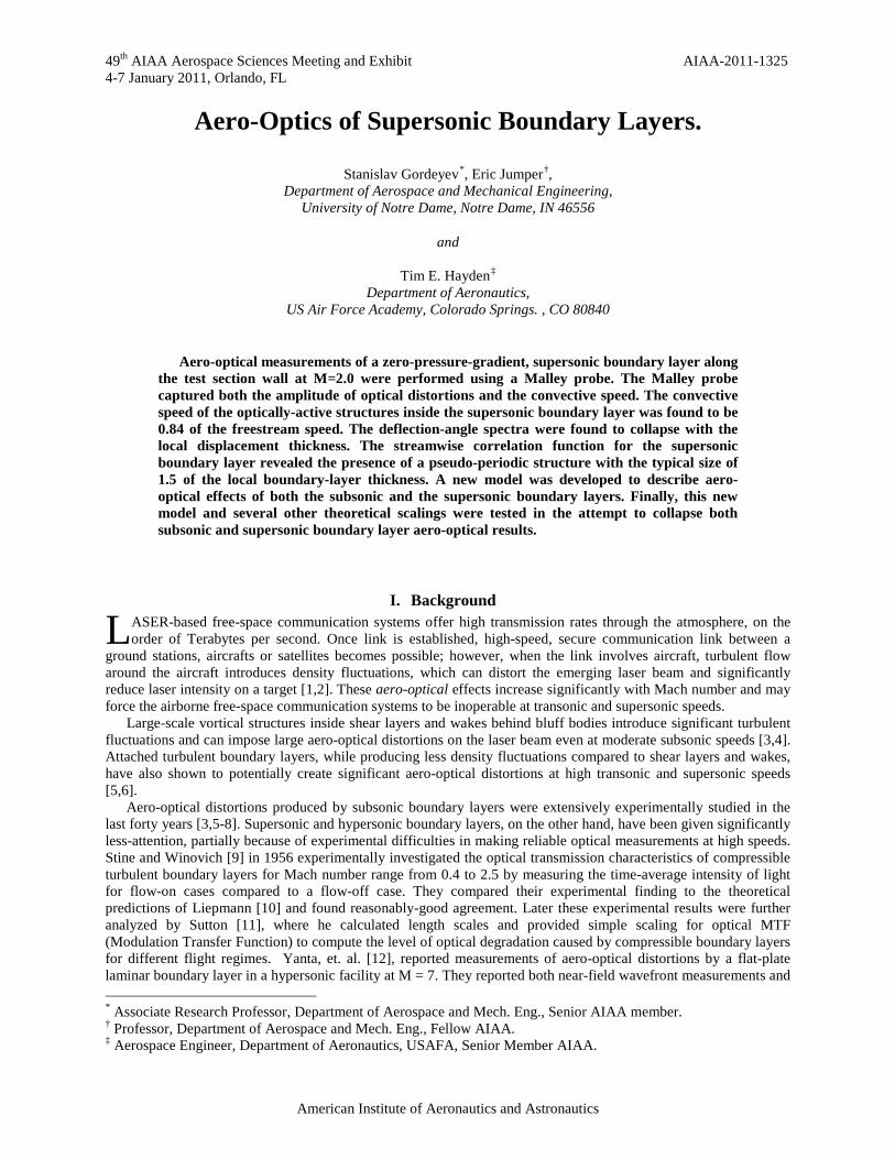
Colorado Springs. The tunnel is an open circuit, blow-down-type facility, with a range of Mach numbers between 0.24 - 4.5. The tunnel is shown schematically in Figure 1, top. Tunnel is passed through several stages of filters and dryers, and is compressed by two rotary screw compressors, 350 hp each to six 900-cubic-foot storage tanks at pressures up to 600 psi. The stored air is heated to approximately 100 deg F to prevent complications due to water condensation and ice formation during high-Mach-number tests. The tunnel has a 1ft x 1 ft cross-section test section with two 12” round optical windows on both sides of the test section, see Figure 1, bottom.

Figure 1. Top: Schematic of the US Air Force Academy Trisonic Wind Tunnel. Bottom: The test section with 1-ft-diameter optical windows.



3

For all tests the freestream Mach number was 2.0; to change the test section static density the plenum pressure was varied between 50 and 100 psi, so the test section static pressure was varied between 6 and 12 psia. The results presented in this paper were obtained with a plenum pressure of 80 psia. The static temperature was estimated to be between -165 F and -160 F for different runs using the total temperature measurements and the isentropic relation.

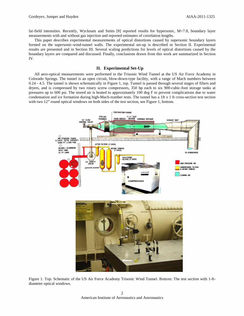
Figure 2. Schematics of Double Boundary Layer (DBL) experimental set-up. All optical measurements were performed using a Malley Probe [13]; the schematic of the experimental set-up are shown in Figure 2 and the optical bench can be seen in the foreground of Figure 1, bottom. The laser beam, after passing through the spatial filter, was re-collimated and split into two small (about a millimeter in diameter) parallel beams, separated in the streamwise direction by a known distance. Beam separation was varied between 6 and 11 mm for different runs. The beams were then forwarded into the test section normal to the optical window. The return mirror on the other side of the test section reflected beams back to the optical bench along the same optical path. The returning beams were split off using a cube beam splitter and, after passing through focusing lens, each beam was focused onto Position Sensing Devices (PDS), capable of measuring instantaneous beam deflections. The sampling frequency was 200 kHz and the sampling time was 10 seconds. During the first test, the laser beams were passed into the empty test section, so they encountered two supersonic boundary layers, one on each sides of the test section. This test is referred to as the double boundary-layer or DBL test. The beams’ streamwise location was varied to investigate the effect of the boundary layer growth along the optical window.

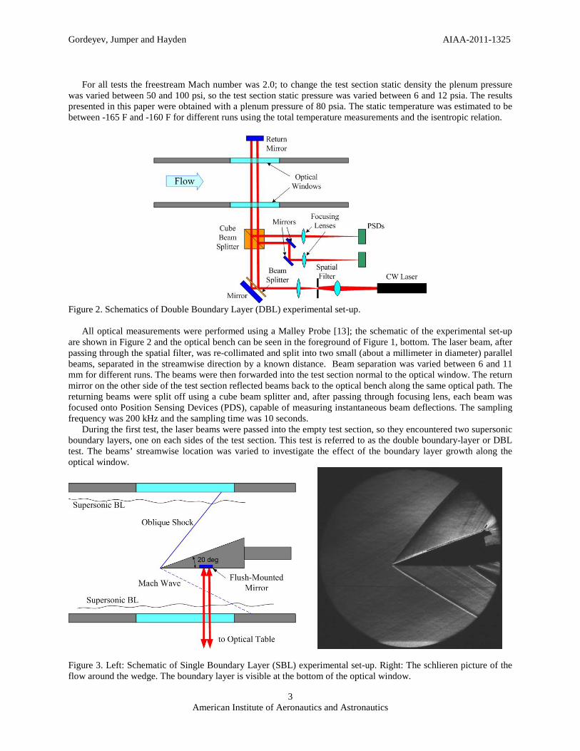
Figure 3. Left: Schematic of Single Boundary Layer (SBL) experimental set-up. Right: The schlieren picture of the flow around the wedge. The boundary layer is visible at the bottom of the optical window.



4

During the second test, a wedge model was placed into the flow, with a mirror mounted flush on the zero-angle

side of the wedge, see Figure 3, left. Both beams were reflected from the small mirror back to the optical table exactly along the same optical path, then split to the PSD’s as before. In this test the beams were traversed through only one boundary layer (and a weak Mach wave generated by the wedge); this test is referred to as the single boundary–layer or SBL test.

In addition to aero-optical tests, schlieren images of the wedge model (rotated 90 degrees) in the test section were taken to visualize the flow pattern around it, see Figure 3, right, and also to estimate the local boundary layer thickness on the test section wall, visible at the bottom of the schlieren image in Figure 2, right. The boundary layer at the center of the test section window was found to be approximately 12 mm thick. The Malley probe measures the instantaneous deflection angle, θ(t), which, assuming the frozen flow hypothesis, is related to the level of optical distortions, OPD(x), as,

dtdOPDU

dtdOPD

dtdx

dxdOPDt c−===)(θ , where Uc is the convective speed of the moving

optical structures. Knowing the beam separation, the convective speed as a function of the frequency is also directly measured by the Malley Probe by spectrally cross-correlating the deflection angles of the two beams [13]. Finally, one-dimensional slices of OPD(t) can be calculated by integrating the deflection angles in time [13],

∫−=−=t

occ dttUtUxOPD )()( θ . (1)

III. Results An example of a deflection-angle spectrum of the

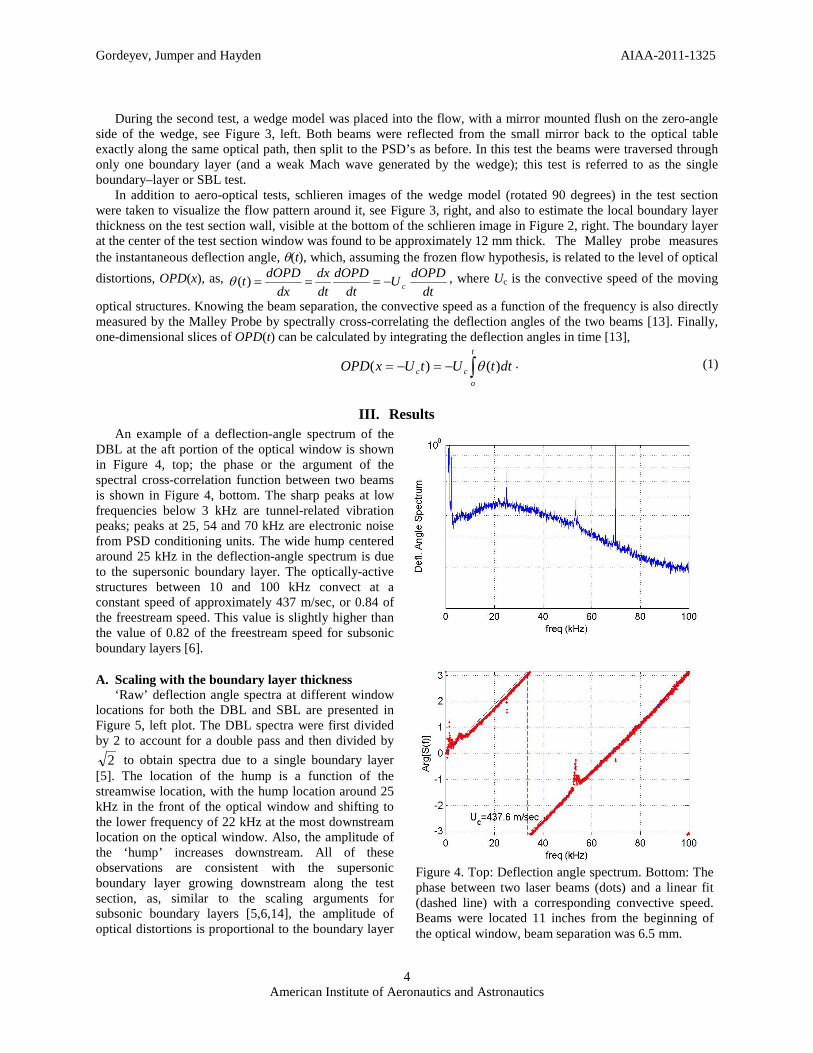
DBL at the aft portion of the optical window is shown in Figure 4, top; the phase or the argument of the spectral cross-correlation function between two beams is shown in Figure 4, bottom. The sharp peaks at low frequencies below 3 kHz are tunnel-related vibration peaks; peaks at 25, 54 and 70 kHz are electronic noise from PSD conditioning units. The wide hump centered around 25 kHz in the deflection-angle spectrum is due to the supersonic boundary layer. The optically-active structures between 10 and 100 kHz convect at a constant speed of approximately 437 m/sec, or 0.84 of the freestream speed. This value is slightly higher than the value of 0.82 of the freestream speed for subsonic boundary layers [6].

A. Scaling with the boundary layer thickness ‘Raw’ deflection angle spectra at different window

locations for both the DBL and SBL are presented in Figure 5, left plot. The DBL spectra were first divided by 2 to account for a double pass and then divided by

2 to obtain spectra due to a single boundary layer [5]. The location of the hump is a function of the streamwise location, with the hump location around 25 kHz in the front of the optical window and shifting to the lower frequency of 22 kHz at the most downstream location on the optical window. Also, the amplitude of the ‘hump’ increases downstream. All of these observations are consistent with the supersonic boundary layer growing downstream along the test section, as, similar to the scaling arguments for subsonic boundary layers [5,6,14], the amplitude of optical distortions is proportional to the boundary layer

Figure 4. Top: Deflection angle spectrum. Bottom: The phase between two laser beams (dots) and a linear fit (dashed line) with a corresponding convective speed. Beams were located 11 inches from the beginning of the optical window, beam separation was 6.5 mm.



5

thickness and the location of the ‘hump’ is inversely proportional to the boundary layer thickness. In [14] it was shown that subsonic boundary layer deflection angle spectra, )(ˆ fθ , scale with the freestream

conditions and the local boundary layer displacement thickness as,

)/(ˆ1)(~)(ˆ **∞

∞ = UfStU

MFf normcSL

δθδρρ

θ , (2)

where ∞ρ and ∞U are the freestream density and the speed, respectively, SLρ = 1.225 kg/m3 is the sea-level

density, dyU

yUy∫∞

∞∞

−=

0

* )()(1ρ

ρδ is the compressible displacement thickness and ∞= UU C 84.0 is the convective

speed of the optical distortions. For subsonic speeds the Mach-dependent function, F(M), was found to be F(M) = M2 ; the Mach-scaling for supersonic speeds will be discussed later in this paper.

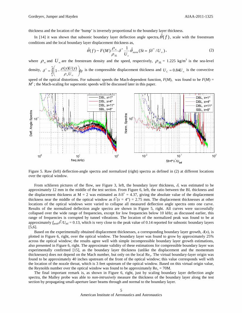
Figure 5. Raw (left) deflection-angle spectra and normalized (right) spectra as defined in (2) at different locations over the optical window.

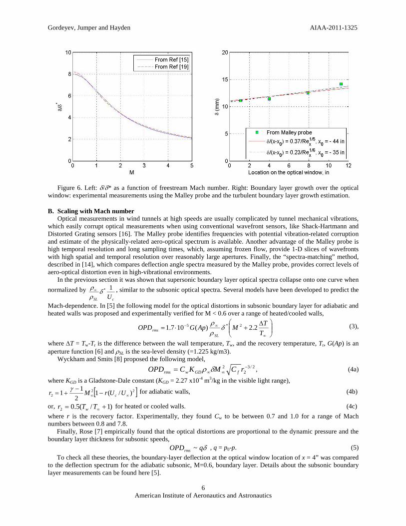
From schlieren pictures of the flow, see Figure 3, left, the boundary layer thickness, δ, was estimated to be approximately 12 mm in the middle of the test section. From Figure 6, left, the ratio between the BL thickness and the displacement thickness at M = 2 was estimated as δ/δ∗ = 4.37, giving the absolute value of the displacement thickness near the middle of the optical window as δ*(x = 4”) = 2.75 mm. The displacement thicknesses at other locations of the optical windows were varied to collapse all measured deflection angle spectra onto one curve. Results of the normalized deflection angle spectra are shown in Figure 5, right. All curves were successfully collapsed over the wide range of frequencies, except for low frequencies below 10 kHz; as discussed earlier, this range of frequencies is corrupted by tunnel vibrations. The location of the normalized peak was found to be at approximately fpeakδ*/Uinf = 0.13, which is very close to the peak value of 0.14 reported for subsonic boundary layers [5,6].

Based on the experimentally obtained displacement thicknesses, a corresponding boundary layer growth, δ(x), is plotted in Figure 6, right, over the optical window. The boundary layer was found to grow by approximately 25% across the optical window; the results agree well with simple incompressible boundary layer growth estimations, also presented in Figure 6, right. The approximate validity of these estimations for compressible boundary layer was experimentally confirmed [15], as the boundary layer thickness (unlike the displacement and the momentum thicknesses) does not depend on the Mach number, but only on the local Rex. The virtual boundary-layer origin was found to be approximately 40 inches upstream of the front of the optical window; this value corresponds well with the location of the nozzle throat, which is 3 feet upstream of the optical window. Based on this virtual origin value, the Reynolds number over the optical window was found to be approximately Rex = 70M.

The final important remark is, as shown in Figure 6, right, just by scaling boundary layer deflection angle spectra, the Malley probe was able to non-intrusively measure the thickness of the boundary layer along the test section by propagating small-aperture laser beams through and normal to the boundary layer.



6

Figure 6. Left: δ/δ* as a function of freestream Mach number. Right: Boundary layer growth over the optical window: experimental measurements using the Malley probe and the turbulent boundary layer growth estimation.

B. Scaling with Mach number Optical measurements in wind tunnels at high speeds are usually complicated by tunnel mechanical vibrations,

which easily corrupt optical measurements when using conventional wavefront sensors, like Shack-Hartmann and Distorted Grating sensors [16]. The Malley probe identifies frequencies with potential vibration-related corruption and estimate of the physically-related aero-optical spectrum is available. Another advantage of the Malley probe is high temporal resolution and long sampling times, which, assuming frozen flow, provide 1-D slices of wavefronts with high spatial and temporal resolution over reasonably large apertures. Finally, the “spectra-matching” method, described in [14], which compares deflection angle spectra measured by the Malley probe, provides correct levels of aero-optical distortion even in high-vibrational environments.

In the previous section it was shown that supersonic boundary layer optical spectra collapse onto one curve when normalized by

cSL U1*δ

ρρ∞ , similar to the subsonic optical spectra. Several models have been developed to predict the

Mach-dependence. In [5] the following model for the optical distortions in subsonic boundary layer for adiabatic and heated walls was proposed and experimentally verified for M < 0.6 over a range of heated/cooled walls,

∆+⋅=

∞

∞−

TTMApGOPD

SLrms 2.2)(107.1 2*5 δ

ρρ (3),

where ∆T = Tw-Tr is the difference between the wall temperature, Tw, and the recovery temperature, Tr, G(Ap) is an aperture function [6] and ρSL is the sea-level density (=1.225 kg/m3).

Wyckham and Smits [8] proposed the following model, 2/3

22 −∞∞= rCMKCOPD fGDwrms δρ , (4a)

where KGD is a Gladstone-Dale constant (KGD = 2.27 x10-4 m3/kg in the visible light range),

[ ]222 )/(1

211 ∞∞ −

−+= UUrMr c

γ for adiabatic walls, (4b)

or, )1/(5.02 += ∞TTr w for heated or cooled walls. (4c) where r is the recovery factor. Experimentally, they found Cw to be between 0.7 and 1.0 for a range of Mach numbers between 0.8 and 7.8.

Finally, Rose [7] empirically found that the optical distortions are proportional to the dynamic pressure and the boundary layer thickness for subsonic speeds,

δqOPDrms ~ , q = p0-p. (5) To check all these theories, the boundary-layer deflection at the optical window location of x = 4” was compared

to the deflection spectrum for the adiabatic subsonic, M=0.6, boundary layer. Details about the subsonic boundary layer measurements can be found here [5].



7

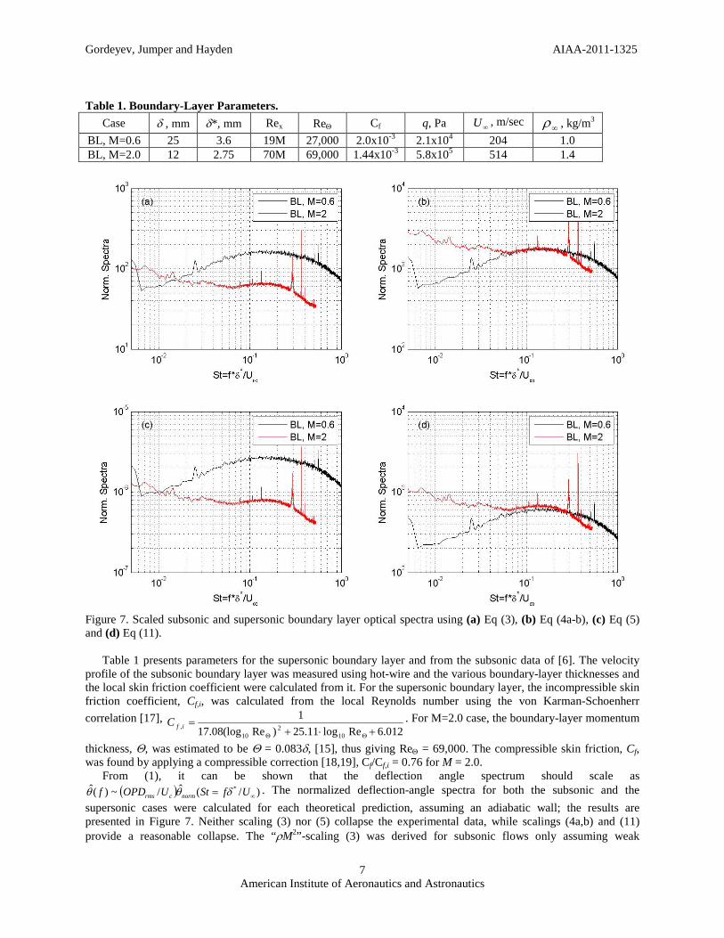
Table 1. Boundary-Layer Parameters.

Case δ , mm δ*, mm Rex ReΘ Cf q, Pa ∞U , m/sec ∞ρ , kg/m3

BL, M=0.6 25 3.6 19M 27,000 2.0x10-3 2.1x104 204 1.0 BL, M=2.0 12 2.75 70M 69,000 1.44x10-3 5.8x105 514 1.4

Figure 7. Scaled subsonic and supersonic boundary layer optical spectra using (a) Eq (3), (b) Eq (4a-b), (c) Eq (5) and (d) Eq (11).

Table 1 presents parameters for the supersonic boundary layer and from the subsonic data of [6]. The velocity

profile of the subsonic boundary layer was measured using hot-wire and the various boundary-layer thicknesses and the local skin friction coefficient were calculated from it. For the supersonic boundary layer, the incompressible skin friction coefficient, Cf,i, was calculated from the local Reynolds number using the von Karman-Schoenherr correlation [17],

012.6Relog11.25)Re(log08.171

102

10, +⋅+

=ΘΘ

ifC . For M=2.0 case, the boundary-layer momentum

thickness, Θ, was estimated to be Θ = 0.083δ, [15], thus giving ReΘ = 69,000. The compressible skin friction, Cf, was found by applying a compressible correction [18,19], Cf/Cf,i = 0.76 for M = 2.0.

From (1), it can be shown that the deflection angle spectrum should scale as ( ) )/(ˆ/~)(ˆ *

∞= UfStUOPDf normcrms δθθ . The normalized deflection-angle spectra for both the subsonic and the supersonic cases were calculated for each theoretical prediction, assuming an adiabatic wall; the results are presented in Figure 7. Neither scaling (3) nor (5) collapse the experimental data, while scalings (4a,b) and (11) provide a reasonable collapse. The “ρM2”-scaling (3) was derived for subsonic flows only assuming weak



8

compressibility and therefore was not expected to work at supersonic speeds. This model was modified to include strong compressibility effects at high Mach numbers, see Eq (11). The full model derivation is presented later in this paper. The “dynamic-pressure” scaling (5) also failed to properly scale the data because the OPD should be proportional to the freestream density, while the dynamic pressure is proportional to the freestream pressure, which is the product of freestream density and temperature. Therefore, OPD cannot be just proportional to q due to dimensional requirements. The test section walls were at approximately Tw = 70F = 294K, while the freestream flow was ∞T = -160F = 166K. Since the running tunnel times were shorter than 30 seconds, it was not long enough to bring the test section walls to thermal equilibrium with the flow; thus the boundary layer for the supersonic-flow case developed over a slightly-heated wall. To estimate the possible heating effect on the aero-optical boundary layer performance, a subsonic approximation for a heated-wall boundary layer was used (3), ( )./)(2.2~ 2

∞∞ −⋅+ TTTMOPD rwrms The

recovery temperature can be estimated as Tr = (1 + r(γ - 1)/2M2) ∞T = 288 K, giving ∞−⋅ TTT rw /)(2.2 ~ 0.08. This term is much smaller than the M2-term, so wall-temperature effects can be ignored for this supersonic boundary layer.

C. Aero-Optical Boundary-Layer Structure From Figure 7(b), it can be observed that the normalized subsonic and supersonic spectra are nearly identical in

the range of normalized frequencies, ∞Uf /*δ , between 0.06 and 0.3. For frequencies ∞Uf /*δ < 0.06, or, in dimensional units, f < 11 kHz, the aero-optical spectrum of the supersonic boundary layer is most probably corrupted by tunnel vibrations, as the phase in this range deviates from the expected straight line, see Figure 4, bottom curve. For high frequencies above, ∞Uf /*δ > 0.3, the supersonic boundary layer aero-optical spectrum is consistently below the subsonic boundary layer spectrum. This frequency range correspond to aero-optical structures with wavelengths, Λ, smaller than ** 8.23.0/)/( δδ ==Λ ∞UU chigh = 7.7 mm. Thus, these small-scale structures are less optically-active than the similar small-scale structures in the subsonic boundary layer.

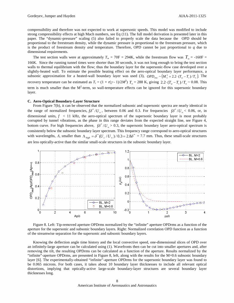
Figure 8. Left: Tip-removed aperture OPDrms normalized by the “infinite” aperture OPDrms as a function of the aperture for the supersonic and subsonic boundary layers. Right: Normalized correlation OPD function as a function of the streamwise separation for the supersonic and subsonic boundary layers.

Knowing the deflection angle time history and the local convective speed, one-dimensional slices of OPD over

an infinitely-large aperture can be calculated using (1). Wavefronts then can be cut into smaller apertures and, after removing the tilt, the resulting OPDrms can be calculated as a function of the aperture. Results normalized by the “infinite”-aperture OPDrms, are presented in Figure 8, left, along with the results for the M=0.6 subsonic boundary layer [6]. The experimentally-obtained “infinite”-aperture OPDrms for the supersonic boundary layer was found to be 0.065 microns. For both cases, it takes about 10 boundary layer thicknesses to include all relevant optical distortions, implying that optically-active large-scale boundary-layer structures are several boundary layer thicknesses long.



9

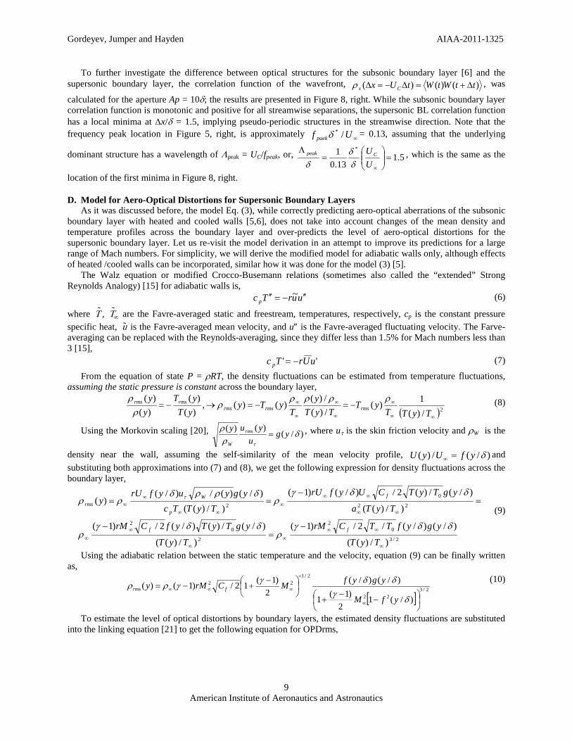
To further investigate the difference between optical structures for the subsonic boundary layer [6] and the supersonic boundary layer, the correlation function of the wavefront, )()()( ttWtWtUx Cx ∆+=∆−=∆ρ , was

calculated for the aperture Ap = 10δ; the results are presented in Figure 8, right. While the subsonic boundary layer correlation function is monotonic and positive for all streamwise separations, the supersonic BL correlation function has a local minima at ∆x/δ = 1.5, implying pseudo-periodic structures in the streamwise direction. Note that the frequency peak location in Figure 5, right, is approximately ∞Uf paek /*δ = 0.13, assuming that the underlying

dominant structure has a wavelength of Λpeak = UC/fpeak, or, 5.113.01 *

=

=

Λ

∞UU Cpeak

δδ

δ, which is the same as the

location of the first minima in Figure 8, right.

D. Model for Aero-Optical Distortions for Supersonic Boundary Layers As it was discussed before, the model Eq. (3), while correctly predicting aero-optical aberrations of the subsonic

boundary layer with heated and cooled walls [5,6], does not take into account changes of the mean density and temperature profiles across the boundary layer and over-predicts the level of aero-optical distortions for the supersonic boundary layer. Let us re-visit the model derivation in an attempt to improve its predictions for a large range of Mach numbers. For simplicity, we will derive the modified model for adiabatic walls only, although effects of heated /cooled walls can be incorporated, similar how it was done for the model (3) [5].

The Walz equation or modified Crocco-Busemann relations (sometimes also called the “extended” Strong Reynolds Analogy) [15] for adiabatic walls is,

uurTc p ′′−=′′ ~ (6)

where

˜ T ,

˜ T ∞ are the Favre-averaged static and freestream, temperatures, respectively, cp is the constant pressure specific heat,

˜ u is the Favre-averaged mean velocity, and u″ is the Favre-averaged fluctuating velocity. The Farve-averaging can be replaced with the Reynolds-averaging, since they differ less than 1.5% for Mach numbers less than 3 [15],

'' uUrTc p −= (7)

From the equation of state P = ρRT, the density fluctuations can be estimated from temperature fluctuations, assuming the static pressure is constant across the boundary layer,

( )2/)(1)(

/)(/)(

)()(,)()(

)()(

∞∞

∞

∞

∞

∞

∞ −=−=→−=TyTT

yTTyT

yT

yTyyTyT

yy

rmsrmsrmsrmsrms ρρρρ

ρρ

ρ (8)

Using the Morkovin scaling [20], )/()()( δ

ρρ

τ

ygu

yuy rms

W

= , where uτ is the skin friction velocity and ρW is the

density near the wall, assuming the self-similarity of the mean velocity profile, )/(/)( δyfUyU =∞ and substituting both approximations into (7) and (8), we get the following expression for density fluctuations across the boundary layer,

2/3

02

2

02

22

0

2

)/)((

)/()/(/2/)1(

)/)((

)/(/)()/(2/)1(

)/)((

)/(/)(2/)/()1(

)/)(()/()(/)/(

)(

∞

∞∞

∞∞

∞

∞

∞∞

∞∞

∞∞∞

∞∞

−=

−

=−

==

TyT

ygyfTTCrM

TyT

ygTyTyfCrM

TyTa

ygTyTCUyfrU

TyTTcygyuyfrU

y

ff

f

p

Wrms

δδγρ

δδγρ

δδγρ

δρρδρρ τ

(9)

Using the adiabatic relation between the static temperature and the velocity, equation (9) can be finally written as,

[ ]2/3

22

2/122

)/(12

)1(1

)/()/(2

)1(12/)1()(

−

−+

−

+−=

∞

=

∞∞∞

δγδδγγρρyfM

ygyfMCrMy frms

(10)

To estimate the level of optical distortions by boundary layers, the estimated density fluctuations are substituted into the linking equation [21] to get the following equation for OPDrms,



10

[ ]

)()0()()0(

)/()/()/(1

2)1(1

)/()/(2

)1(12/)1(2

12

2/1

0

2

2/322

2/122

∞∞∞

∞∞

∞

∞

=

∞∞∞

==

Λ

−

−+

−

+−= ∫

MFCBKC

MCCMKCOPD

ydyyfM

ygyfMCrMKOPD

fGDfGDrms

yfGDrms

δρδρ

δδδ

δγδδγγδρ ,(11)

where

[ ]

Λ

−

−+

−

+−= ∫∞

∞

=

∞∞0

2

2/322

2/12 )/()/(

)/(12

)1(1

)/()/(2

)1(1)1()( δδδ

δγδδγγ ydyyfM

ygyfMrMC y , (12)

B = C(0), )0(/)()( 21 CMCMMF ∞∞∞ = and )/()1( δyyΛ and )/()2( δyyΛ two different wall-normal density

correlations lengths, )/()1( δyyΛ is provided by Gilbert [22] and )/()2( δyyΛ is measured by Rose and Johnson [23].

Note, that both the model (11) and the model (4a,b) have the same functional form, fGDrms CKOPD δρ∞~ ,

but a different Mach-number-dependent function, )(1 ∞MF for the modified model Eq. (11) and

[ ]2/3

2222 )/(1

211)(

−

∞∞∞∞

−

−+= UUrMMMF c

γ for the model Eq. (4a,b). To calculate )(1 ∞MF from (12),

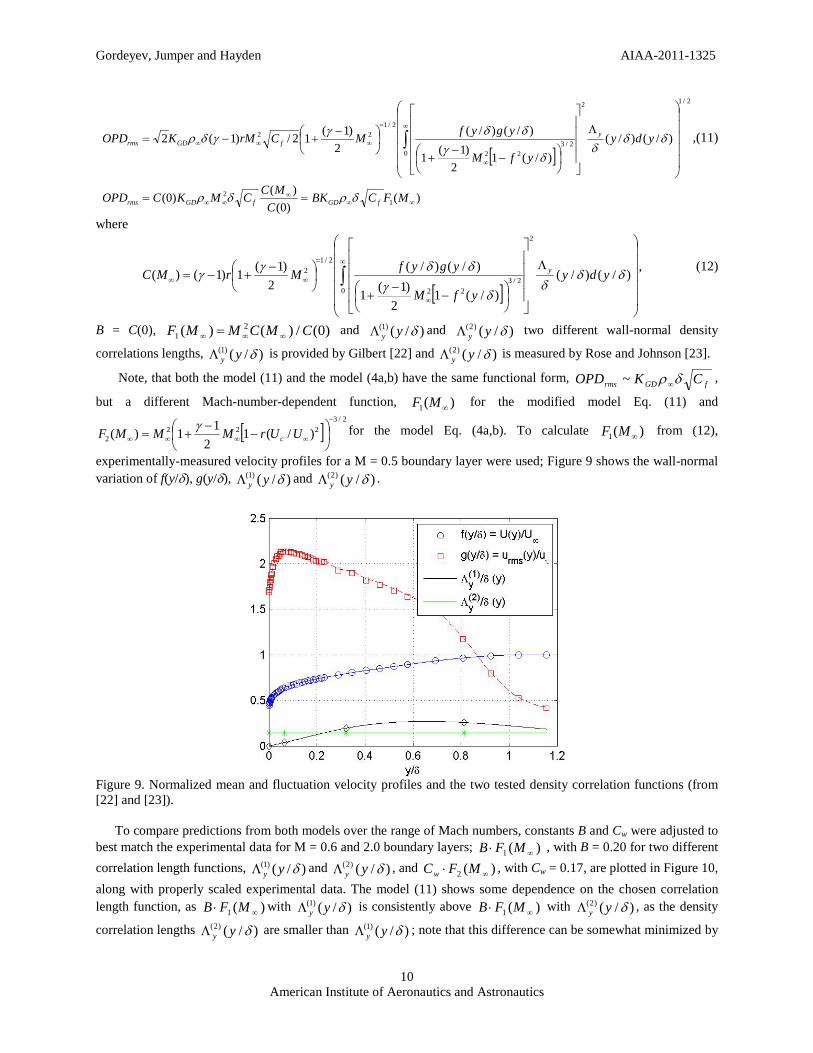
experimentally-measured velocity profiles for a M = 0.5 boundary layer were used; Figure 9 shows the wall-normal variation of f(y/δ), g(y/δ), )/()1( δyyΛ and )/()2( δyyΛ .

Figure 9. Normalized mean and fluctuation velocity profiles and the two tested density correlation functions (from [22] and [23]). To compare predictions from both models over the range of Mach numbers, constants B and Cw were adjusted to best match the experimental data for M = 0.6 and 2.0 boundary layers; )(1 ∞⋅ MFB , with B = 0.20 for two different correlation length functions, )/()1( δyyΛ and )/()2( δyyΛ , and )(2 ∞⋅ MFCw , with Cw = 0.17, are plotted in Figure 10, along with properly scaled experimental data. The model (11) shows some dependence on the chosen correlation length function, as )(1 ∞⋅ MFB with )/()1( δyyΛ is consistently above )(1 ∞⋅ MFB with )/()2( δyyΛ , as the density

correlation lengths )/()2( δyyΛ are smaller than )/()1( δyyΛ ; note that this difference can be somewhat minimized by



11

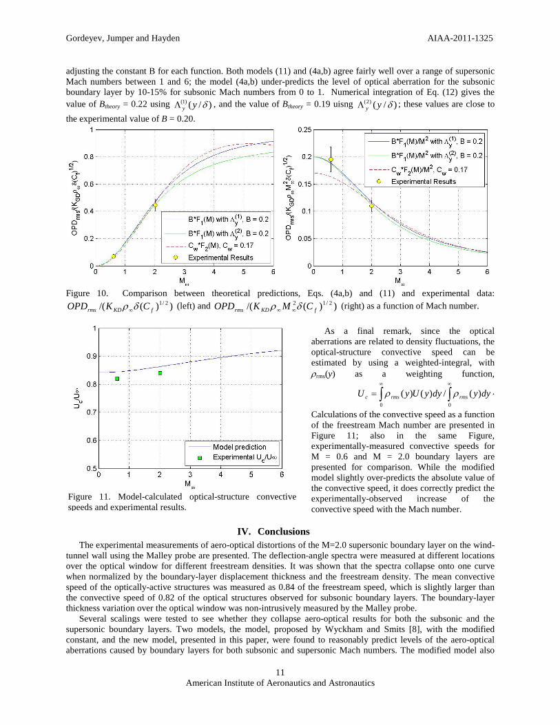
adjusting the constant B for each function. Both models (11) and (4a,b) agree fairly well over a range of supersonic Mach numbers between 1 and 6; the model (4a,b) under-predicts the level of optical aberration for the subsonic boundary layer by 10-15% for subsonic Mach numbers from 0 to 1. Numerical integration of Eq. (12) gives the value of Btheory = 0.22 using )/()1( δyyΛ , and the value of Btheory = 0.19 uisng )/()2( δyyΛ ; these values are close to the experimental value of B = 0.20.

Figure 10. Comparison between theoretical predictions, Eqs. (4a,b) and (11) and experimental data:

))(/( 2/1fKDrms CKOPD δρ∞ (left) and ))(/( 2/12

fKDrms CMKOPD δρ ∞∞ (right) as a function of Mach number. As a final remark, since the optical aberrations are related to density fluctuations, the optical-structure convective speed can be estimated by using a weighted-integral, with ρrms(y) as a weighting function,

∫∫∞∞

=00

)(/)()( dyydyyUyU rmsrmsc ρρ .

Calculations of the convective speed as a function of the freestream Mach number are presented in Figure 11; also in the same Figure, experimentally-measured convective speeds for M = 0.6 and M = 2.0 boundary layers are presented for comparison. While the modified model slightly over-predicts the absolute value of the convective speed, it does correctly predict the experimentally-observed increase of the convective speed with the Mach number.

IV. Conclusions The experimental measurements of aero-optical distortions of the M=2.0 supersonic boundary layer on the wind-tunnel wall using the Malley probe are presented. The deflection-angle spectra were measured at different locations over the optical window for different freestream densities. It was shown that the spectra collapse onto one curve when normalized by the boundary-layer displacement thickness and the freestream density. The mean convective speed of the optically-active structures was measured as 0.84 of the freestream speed, which is slightly larger than the convective speed of 0.82 of the optical structures observed for subsonic boundary layers. The boundary-layer thickness variation over the optical window was non-intrusively measured by the Malley probe. Several scalings were tested to see whether they collapse aero-optical results for both the subsonic and the supersonic boundary layers. Two models, the model, proposed by Wyckham and Smits [8], with the modified constant, and the new model, presented in this paper, were found to reasonably predict levels of the aero-optical aberrations caused by boundary layers for both subsonic and supersonic Mach numbers. The modified model also

Figure 11. Model-calculated optical-structure convective speeds and experimental results.



12

correctly predicted the experimentally-observed increase of the normalized convective speeds with the increasing Mach number. Other models, while correctly predicting the ‘ρM2’-dependence of the aero-optical distortions at subsonic speeds, did not correctly include high-Mach-number compressibility effects and therefore failed at supersonic speeds. The small-scale structures in the M = 2.0 supersonic boundary layer were found to be less-optically-active, compared to the subsonic boundary layer. From the streamwise correlation measurements it was found that the dominant optical structure in the supersonic boundary layer is weakly-periodic, with the typical length of 1.5 of the boundary layer thickness. The minimum aperture size was found to be at least 10 boundary-layer thicknesses to include all aero-optical effects from the boundary layer; a similar aperture size was observed for the subsonic boundary layer. Smaller apertures will undoubtedly decrease the observed level of aero-optical distortions and will change the apparent correlation length of the underlying optical structure. All these conclusions are based on experimental data taken at one supersonic Mach number only, so all high-Mach-number trends presented in this paper should be treated as preliminary. More measurements at different supersonic Mach numbers should be taken to better understand the optical degradation caused by supersonic boundary layers.

Acknowledgments The authors would like to thank SSgt Danny Washburn for providing assistance in the Trisonic Tunnel measurements, especially schlieren set-up. They also thank Director for Aeronautics Research Center, USAFA, Thomas McLaughlin for providing opportunity to conduct reported measurements.

This work was partially funded by AFOSR, Grant FA9550-09-1-0449. The U.S. Government is authorized to reproduce and distribute reprints for government purposes notwithstanding any copyright notation thereon.

References [1] Gilbert, J. and Otten, L.J. (eds), Aero-Optical Phenomena, Progress in Astronautics and Aeronautics, Vol, 80,

AIAA, New York, 1982. [2] Jumper, E.J. and Fitzgerald, E.J., “Recent advances in aero-optics,” Progress in Aerospace Sciences, Vol. 37,

No. 3, 2001, pp. 299-339. [3] Sutton, G.W., “Aero-Optical Foundations and Applications, AIAA Journal, Vol. 23, pp. 1525-1537, 1985. [4] S. Gordeyev and E. Jumper, “Fluid Dynamics and Aero-Optics of Turrets”, Progress in Aerospace Sciences, 46,

(2010), pp. 388-400. [5] J. Cress, S. Gordeyev and E. Jumper "Aero-Optical Measurements in a Heated, Subsonic, Turbulent Boundary

Layer" , 48th Aerospace Science Meeting and Exhibit, Orlando, Florida, 4-7 Jan, 2010, AIAA Paper 2010-0434. [6] J. A. Cress, Optical Distortions Caused by Coherent Structures in a Subsonic Compressible, Turbulent

Boundary Layer, Ph.D Thesis, University of Notre Dame, 2010. [7] Rose, W.C., “Measurements of Aerodynamic Parameters Affecting Optical Performance,” Air Force Weapons

Laboratory Final Report, AFWL-TR-78-191, May 1979. [8] C. Wyckham, and A. Smits, “Aero-Optic Distortion in Transonic and Hypersonic Turbulent Boundary Layers“,

AIAA Journal, 47(9), pp. 2158-2168, 2009. [9] Stine HA, Winovich W. Light diffusion through high-speed turbulent boundary layers. Research Memorandum

A56B21, NACA, Washington, May 1956. [10] H. W. Liepmann, Deflection and diffusion of a light ray passing through a boundary layer, Technical Report

SM-14397, Douglas Aircraft Company, Santa Monica Division, 16 May 1952. [11] Sutton, G.W. “Optical Imaging Through Aircraft Turbulent Boundary Layers”, Progress in Astronautics and

Aeronautics: Aero-Optical Phenomena, Vol. 80, edited by K. Gilbert and L.J. Otten, AIAA, New York, pp. 15-39, 1982.

[12] Yanta, W.J., Spring, W.C.III, Lafferty, J.F., Collier, A.S., Bell, R.L., Neal, D.R., Hamrick, D.R., Copland, R.J., Pezzaniti, L., Banish, M. and Shaw, R., “Near- and Farfield Measurements of Aero-Optical Effects Due To Propagation Through Hypersonic Flows”, 31st AIAA Plasmadynamics and Lasers Conference, Denver, CO, 19-22 June, 2000, AIAA Paper 2000-2357.

[13] S. Gordeyev, T. Hayden and E. Jumper, "Aero-Optical and Flow Measurements Over a Flat-Windowed Turret”, AIAA Journal, vol. 45, No. 2, pp. 347-357, 2007.

[14] D. Wittich, S. Gordeyev and E. Jumper, “Revised Scaling of Optical Distortions Caused by Compressible, Subsonic Turbulent Boundary Layers”, 38th AIAA Plasmadynamics and Lasers Conference, Miami, Florida, 25-28 June, 2007, AIAA Paper 2007-4009.



13

[15] Smits, A.J and Dussauge, J.-P., Turbulent Shear Layers in Supersonic Flow, American Institute of Physics, Woodbury, New York, 1996.

[16] S. Gordeyev, E. Jumper, B. Vukasinovic, A. Glezer and V. Kibens "Hybrid Flow Control of a Turret Wake, Part II: Aero-Optical Effects" , 48th Aerospace Science Meeting and Exhibit, Orlando, Florida, 4-7 Jan, 2010, AIAA Paper 2010-0438.

[17] Bardina, J. E., Huang, P. G. and Coakley, T. J., Turbulence Modeling Validation, Testing, and Development, NASA Tech. Mem. 110446, 1980.

[18] Eckett, E.R.G., “Engineering Relations for Friction and Heat Transfer to Surfaces in High Velocity Flow”, Journal of the Aeronautical Sciences, 22(8), pp. 585-587, 1955.

[19] Stratford, B.S. and Beaver, G.S., The Calculation of the Compressible Turbulent Boundary layer in an Arbitrary Pressure Gradient – A Correlation of Certain Previous Methods, Reports and Memoranda No. 3207, Ministry of Aviation, Aeronautical Research Council, London, 1961.

[20] Morkovin, M.V., Effects of compressibility on turbulent flows, Mechanique de la Turbulence, edited by Favre, A.J., pp. 367-380, 1962.

[21] Sutton, G.W., “Effect of Turbulent Fluctuations in an Optically Active Fluid Medium,” AIAA Journal, Vol. 7, No. 9, September 1969, pp. 1737-1743.

[22] Gilbert, K.G., “KC-135 Aero-Optical Boundary-Layer/Shear-Layer Experiments,” Aero-Optical Phenomena, Eds. K.G. Gilbert and L.J. Otten, Vol. 80, Progress in Astronautics and Aeronautics, AIAA, New York, 1982, pp. 306-324.

[23] Rose, W.C. and Johnson, E.A., “Unsteady Density and Velocity Measurements in the 6 x 6 ft Wind Tunnel”, Progress in Astronautics and Aeronautics: Aero-Optical Phenomena, Vol. 80, edited by K. Gilbert and L.J. Otten, AIAA, New York, pp. 218-232, 1982.

Documents

Aero-Optics of Supersonic Boundary Layers