Embed Size (px)
Citation preview
AER1301: Kinetic Theory of Gases
Supplementary Notes
Instructor:
Prof. Clinton P. T. Groth†
University of Toronto Institute for Aerospace Studies
4925 Dufferin Street, Toronto, Ontario, Canada M3H 5T6
January 8, 2007
1 Course Summary
The course is intended to provide an introduction to the kinetic theory of gases. Material coveredin the course includes
• discussion of significant length dimensions;
• different flow regimes, continuum, transition, collision-free;
• a brief history of gas kinetic theory;
• equilibrium kinetic theory, the particle distribution function, Maxwell-Boltzmann distribu-tion.
• collision dynamics, collision frequency and mean free path;
• elementary transport theory, transport coefficients, mean free path method
• Boltzmann equation, derivation, Boltzmann H-theorem, collision operators;
• Generalized transport theory, Maxwell’s equations of change, approximate solution tech-niques, Chapman-Enskog perturbative and Grad series expansion methods, moment closures;
• derivation of the Euler and Navier-Stokes equations, higher-order closures;
• free molecular aerodynamics;
• shock waves.
The textbook for the course is Gaskinetic Theory, by Tamas Gombosi [1]. These notes are intendedto supplement the material covered in the textbook.
†E-mail: [email protected]
1
2 Course Outline
2.1 Outline of Textbook
The material covered in the textbook by Gombosi [1] can be summarized as follows:
• CHAPTER 1: INTRODUCTION
+ Chapter 1 provides a brief history of gaskinetic theory and discusses the evolution fromhydrostatics, to fluid dynamics (hydrodynamics), on through to kinetic theory.
+ Basic assumptions and limitations of kinetic theory:
∗ Molecular Hypothesis: i) matter is composed discrete molecules (particles); ii) allmolecules for a given substance are alike and are the smallest quantity of the sub-stance that retains its unique chemical properties.
∗ Ideal (Perfect) Gases: i) molecules are point-like structures with no internal struc-ture or internal degrees of freedom (monatomic gas assumption); ii) molecules onlyexert forces on one another within the sphere of influence; iii) outside the sphereof influence, motion of molecules described by classical mechanics (non-relativisticequations of motion).
∗ Statistical Nature of Theory: i) individual motion of each molecule is not tracked; ii)particle phase space velocity distribution function, f or F , describes the probabilityof or number of particles having a velocity, v, at position x.
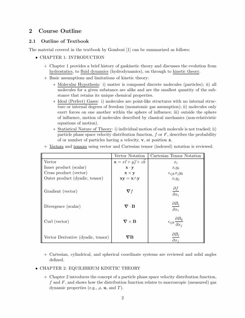
+ Vectors and tensors using vector and Cartesian tensor (indexed) notation is reviewed.
Vector Notation Cartesian Tensor Notation
Vector x = x~ı + y~ + z~k xi
Inner product (scalar) x · y xiyi
Cross product (vector) x × y ǫijkxjyk
Outer product (dyadic, tensor) xy = x∧y xiyj
Gradient (vector) ∇f∂f
∂xi
Divergence (scalar) ∇ ·B ∂Bi
∂xi
Curl (vector) ∇ × B ǫijk∂Bk
∂xj
Vector Derivative (dyadic, tensor) ∇B∂Bi
∂xj
+ Cartesian, cylindrical, and spherical coordinate systems are reviewed and solid anglesdefined.
• CHAPTER 2: EQUILIBRIUM KINETIC THEORY
+ Chapter 2 introduces the concept of a particle phase space velocity distribution function,f and F , and shows how the distribution function relates to macroscopic (measured) gasdynamic properties (e.g., ρ, u, and T ).
2
+ Maxwell-Boltzmann Distribution Function:
F◦ = M =ρ
m (2πp/ρ)3/2exp
(
−1
2
ρc2
p
)
=ρ
m (2πθ)3/2exp
(
−1
2
c2
θ
)
∗ Maxwell’s original derivation of the velocity distribution function under conditions ofthermodynamic equilibrium is reviewed. Notion of drifting Maxwellians is discussedwith c = v− u and where the average (bulk) velocity is
u =m
ρ< vF >=< vf >
∗ Distribution of Molecular Speeds:
f∗(v) = 4πv2(
m
2πkT
)3/2
exp
(
−1
2
mv2
kT
)
∗ Most Probable and Average Speeds:
vm =
(
2kT
m
)1/2
v =
(
8kT
πm
)1/2
+ Specific heats and equipartition of translational energy for a monatomic gas.
- Equilibrium distribution function for a mixture and Dalton’s law.
- Specific heats for a diatomic gas.
• CHAPTER 3: BINARY COLLISIONS
+ Collisional processes are responsible for establishing thermodynamic equilibrium. Theyare also the microscopic processes governing all macroscopic transport phenomena.Chapter 3 provides a thorough description of binary collision process (i.e., the collisionsof two particles).
+ Kinematics of Two-Particle Collisions: center of mass, particle motion in a central forcefield, angle of deflection, inverse power inter-particle potentials.
+ Statistical Description of Collisions: collision frequency, mean free time, mean free path,collision cross section.
ν =√
2nσv τ =1
νλ = vτ =
v
ν=
1√2nσ
- Collision rates for gas mixtures.
- Chemical reactions.
• CHAPTER 4: ELEMENTARY TRANSPORT THEORY
+ Elementary theories for describing non-equilibrium transport are reviewed in Chapter 4.
+ Molecular Effusion: escape from a container through a small orifice.
∗ Hydrodynamic escape.
∗ Kinetic effusion.
jkin =1
4nv
3
+ Fluid Dynamic (Macroscopic) Transport:
∗ Diffusion (Mass Diffusion): Fick’s Law
ji = −D∂n
∂xi
∗ Viscous Drag (Diffusion of Momentum): Viscosity and Fluid Stresses
τij = µ
[(
∂ui
∂xj+
∂uj
∂xi
)
− 2
3δij
∂uα
∂xα
]
∗ Heat Flow (Thermal Diffusion): Fourier’s Law
qi = −κ∂T
∂xi
+ Mean Free Path Method: Assumption that the characteristic length scales are muchlarger than the mean free path, λ. Provides expressions for the fluid dynamic transportcoefficients (i.e., diffusion coefficient, D, viscosity, µ, and thermal conductivity, κ).
+ Flow in a Tube:
∗ Knudsen Number:
Kn =λ
ℓ
∗ Poiseuille Flow (Kn < 0.01).
∗ Slip Flow (0.01 < Kn < 0.1).
∗ Free Molecular Flow (Kn > 10 − 100).
• CHAPTER 5: THE BOLTZMANN EQUATION
+ Chapter 5 provides a derivation of the Boltzmann equation and discusses some of itsmathematical properties.
+ Derivation of the Boltzmann Equation:
∗ Underlying Assumptions: i) the effective range of the inter-molecular forces are muchsmaller than the mean free path; and ii) molecular chaos (colliding particles areuncorrelated and undergo many collisions with other particles before re-colliding).The latter leads to irreversibility in solutions of the Boltzmann equation.
∂F
∂t+ vi
∂F
∂xi+ ai
∂F
∂vi=
δF
δt
+ Boltzmann’s H-Theorem:dH
dt≤ 0
+ Equilibrium distribution and five summation invariant quantities (mass, momentum,energy).
+ Relaxation Time Approximation for the Collision Operator (BGK Model):
δF
δt= −F −M
τ
4
- Relaxation Time Approximation for the Collision Operator (multi-species).
- Fokker-Planck Approximation for the Collision Operator.
• CHAPTER 6: GENERALIZED TRANSPORT EQUATIONS
+ Approximate techniques for constructing general non-equilibrium solutions to the Boltz-mann equation invariably give rise to generalized transport equations. Chapter 6 pro-vides a description of Grad-type moment closure methods and the resulting transportequations which arise. The latter must be solved in place of directly solving the Boltz-mann equation. It is important to note that moment closure methods provide a meansfor constructing approximate non-equilibrium solutions to the Boltzmann equation.
+ Moments of the Boltzmann Equation and Maxwell’s Equations of Change:
∗ Conserved and non-conserved forms of Maxwell’s equations of change.
+ Grad-Type Moment Closures:
∗ 20-Moment Closure (ρ, ui, Pij , Qijk).
Rijkl =1
ρ{PijPkl}(3)
[ijkl] −1
ρ{(pδij − Pij) (pδkl − Pkl)}(3)
[ijkl]
∗ 13-Moment Closure (ρ, ui, Pij , qi).
Qijk =2
5(δijqk + δikqj + δjkqi )
∗ 10-Moment Closure (ρ, ui, Pij).Qijk = 0
∗ 8-Moment Closure (ρ, ui, p, qi).
Pij = δijp Qijk =2
5(δijqk + δikqj + δjkqi )
∗ 5-Moment Closure (ρ, ui, p): Euler equations and assumption of local thermody-namics equilibrium (LTE).
Pij = δijp Qijk = 0
+ BGK Collision Terms for 13-Moment Closure (single species):
δρ
δt=
δui
δt=
δp
δt= 0
δPij
δt= −1
τ(Pij − pδij)
δτij
δt= −τij
τ
δqi
δt= −qi
τ
+ Recovery of Navier-Stokes Equations: 20- and 13-moment closures contain Navier-Stokes equations.
- Collision Terms for Multi-Species Gases.
• CHAPTER 7: FREE MOLECULAR AERODYNAMICS
5
+ For free molecular flows, it is assumed that the mean free path is much larger than thelargest characteristic scale of the flow geometry. Under this assumption, the interactionof the gas molecules can be completely neglected and only the interaction of the gaswith solid surfaces must be taken into account. Free molecular flow theory is reviewedin Chapter 7.
+ Flux of Mass, Momentum, and Translational Energy at a Solid Body:
∗ Reflection Coefficients.
∗ Mass Transfer.
∗ Perpendicular Momentum Transfer.
∗ Tangential Momentum Transfer.
∗ Translational Energy Transfer.
+ Free Molecular Heat Transfer:
∗ Heat transfer between two plates.
+ Free Molecular Aerodynamic Forces:
∗ Pressure and shearing forces.
- Free Molecular Heat Transfer to Specific Bodies.
∗ Stanton number and thermal recovery factor.
- Free Molecular Aerodynamic Forces for Specific Bodies.
∗ Lift and drag forces.
• CHAPTER 8: SHOCK WAVES
+ The structure of steady one-dimensional planar shocks are studied using fluid dynamicand simple kinetic descriptions in Chapter 8.
+ Shock-Wave Solutions:
∗ Fluid dynamics: Euler equations.
∗ Fluid dynamics: Navier-Stokes equations.
∗ Kinetic theory: Mott-Smith model.
Subjects denoted with a “+” sign are core material that you will be responsible for in the final examand subjects denoted with a “-” sign are additional course material that you will not be examinedon.
2.2 Some Additional References
A list of additional references dealing with the subject matter covered in this course are givenbelow. Students are encouraged to consult these references to supplement the material covered inthe course textbook.
• Textbook: Gaskinetic Theory, by T. I. Gombosi, Cambridge University Press, 1994.
• An Introduction to Thermodynamics, the Kinetic Theory of Gases, and Statistical Mechanics,by F. W. Sears, Addison-Wesley, 1950.
• Molecular Flow of Gases, by G. N. Paterson, John Wiley and Sons, 1956.
6
• The Mathematical Theory of Non-Uniform Gases, by S. Chapman and T. G. Cowling, Cam-bridge University Press, 1960.
• An Introduction to the Kinetic Theory of Gases, by J. H. Jeans, Cambridge University Press,1962.
• Introduction to Physical Gas Dynamics, by W. G. Vincenti and C. H. Kruger, John Wileyand Sons, 1965.
• Flow Equations for Composite Gases, by J. M. Burgers, Academic Press, 1969.
• Rarefied Gas Dynamics, by M. N. Kogan, Plenum Press, 1969.
• An Introduction to the Theory of the Boltzmann Equation, by S. Harris, Holt, Rinehart, andWinston, 1971.
• Fundamentals of Maxwell’s Kinetic Theory of a Simple Monatomic Gas, Treated as a Branch
of Rational Mechanics, by C. Truesdell and R. G. Muncaster, Academic Press, 1980.
• Molecular Nature of Aerodynamics, by G. N. Patterson, UTIAS, 1981.
• Extended Thermodynamics, by I. Muller and T. Ruggeri, Springer-Verlag, 1993.
• The Mathematical Theory of Dilute Gases, by C. Cercignani, R. Illner, M. Pulvirenti,Springer-Verlag, 1994.
• Molecular Gas Dynamics and the Direct Simulation of Gas Flows, by G. A. Bird, OxfordScience Publications, 1995.
• Ionospheres: Physics, Plasma Physics, and Chemistry, by R. W. Schunk and A. F. Nagy,Cambridge University Press, 2000.
3 Flow Regimes for a Monatomic Gas
3.1 Knudsen Number
The Knudsen number, Kn, is a measure of a gas’ potential to maintain conditions of thermodynamicequilibrium. It is defined as the ratio of the mean free path (the average distance traveled by a gasparticle between collisions, λ) to an appropriate reference length scale, ℓ, characterizing the flow:
Kn =λ
ℓ. (1)
When the mean free path is small compared with the characteristic length scale or dimension ofinterest (i.e., for Kn ≪ 1), the gas will undergo a large number of collisions over typical lengthscales of interest and assumptions of near thermal equilibrium apply. For such flows the continuumhypothesis is valid and conventional fluid dynamic (macroscopic) descriptions for the fluid behaviour(i.e., the Navier-Stokes equations) are appropriate. Note that on average gas particles must undergoonly about 3 to 4 binary collisions to equilibriate the translational energy modes. When themean free path becomes comparable to or larger than the characteristic length scale (i.e., forKn ≈ 1 and Kn > 1), the gas is unable to maintain conditions of thermal equilibrium and thecontinuum hypothesis fails. As a consequence, fluid dynamic descriptions based on assumptions ofnear equilibrium break down. For such flows, a microscopic description for the fluid behaviour isrequired as may be provided by gas kinetic theory and the Boltzmann equation.
7
3.2 Continuum, Slip, Transition, and Free-Molecular Flow Regimes
Depending on inter-particle collision rate, and hence the flow Knudsen number, four flow regimesmay be identified for a monatomic gas. These four flow regimes and the ranges in the Knudsennumber which define each regime are listed below.
• Continuum Regime
– Kn ≤ 0.01
– collision-dominated flow
– conventional fluid-dynamic equations (i.e., the Navier-Stokes Equations) are valid
• Slip-Flow Regime
– 0.01 < Kn ≤ 0.1
– fluid dynamic equations can be augmented with slip boundary conditions for the flowvelocity and temperature
– Knudsen layer analyses are generally used to formulate appropriate boundary conditions
• Transition Regime
– 0.1 < Kn ≤ 10–100
– collisions are less frequent but cannot be neglected
– very difficult regime to model
• Free-Molecular Flow Regime
– Kn > 10–100
– collisionless flow
– inter-particle collisions negligible, must only consider particle interactions with flow fieldboundaries
Note that values for the Knudsen numbers defining the boundaries between the four regimes givenabove are not sharp and the values listed are typical values that can be used as guides for deter-mining when non-equilibrium rarefied flow effects are important.
In general, the mean free path is related to the fluid viscosity, µ. For hard sphere collisions(described in the course textbook), the mean free path is given by
λ =16µ
5ρ
1√2πRT
, (2)
where ρ, T , and R are the density, temperature, and gas constant. This expression can be used toevaluate the flow Knudsen number given a characteristic length scale. ℓ.
Some simple analysis can be used to relate the Knudsen number, Kn, to the Reynolds numberRe = ρuℓ/µ and Mach number M = u/a, where a =
√γRT is the sound speed for the gas and γ
is the specific heat ratio. For flows for which the Reynolds number is in the range 0 < Re < 100such that inertial terms are relatively small compared with viscous forces, one can write
M =u
a=
u
a
Reµ
ρuℓ=
µ
ρaℓRe ≈ ρaλ
ρaℓRe = KnRe , (3)
8
10−2 0.1 1 10 102 104 105 106 10810−4
10−2
0.1
1
10
102
104
Newtonian flow (M = ∞)
incompressible flow (M = 0)
visc
ous,
ine
rtia
lles
s fl
ow (
Re
= 0
)
invi
scid
flo
w (
Re
= ∞
)
CONTINUUM
FLOW
TRAN
SITIO
NA
L FLO
W
TRANSITIONAL FLOW
FREE-MOLECULAR
FLOW
spaceflight
aeronautics
meteorologymicrometerology
M =
1Re l
M = 1Re x1/2
M =
1 3−1Re x
4/5
M =
0.0
1Re l
M = 0.01Re x1/2
M =
1 3−0.01Re x
4/5
Kn = 1boundary
Kn = 0.01boundary
M
subs
onic
flo
wsu
pers
onic
flo
w
tran
soni
cfl
owco
mpr
essi
bili
tyne
glig
ible
hype
rson
icfl
ow
Re
Stokes flow(inertia negligible)
Oseen flow(viscous fluid)
laminarboundary layer
turbulentboundary layer
symmetric flow asymmetric flow
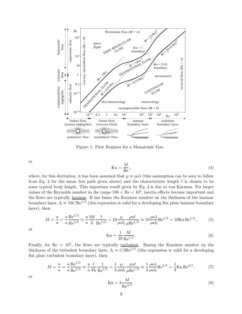
Figure 1: Flow Regimes for a Monatomic Gas.
or
Kn =M
Re, (4)
where, for this derivation, it has been assumed that µ ≈ ρaλ (this assumption can be seen to followfrom Eq. 2 for the mean free path given above) and the characteristic length ℓ is chosen to besome typical body length. This important result given by Eq. 4 is due to von Karman. For largervalues of the Reynolds number in the range 100 < Re < 105, inertia effects become important andthe flows are typically laminar. If one bases the Knudsen number on the thickness of the laminarboundary layer, δl ≈ 10ℓ/Re1/2 (this expression is valid for a developing flat plate laminar boundarylayer), then
M =u
a=
u
a
Re1/2
Re1/2≈ u
a
10ℓ
δl
1
Re1/2= 10
µ
ρaδl
ρuℓ
µRe1/2≈ 10
ρaλ
ρaδlRe1/2 = 10Kn Re1/2 , (5)
or
Kn =1
10
M
Re1/2. (6)
Finally, for Re > 105, the flows are typically turbulent. Basing the Knudsen number on thethickness of the turbulent boundary layer, δt ≈ ℓ/3Re1/5 (this expression is valid for a developingflat plate turbulent boundary layer), then
M =u
a=
u
a
Re1/5
Re1/5≈ u
a
ℓ
3δt
1
Re1/5=
1
3
µ
ρaδt
ρuℓ
µRe1/5≈ 1
3
ρaλ
ρaδtRe4/5 =
1
3Kn Re4/5 , (7)
or
Kn = 3M
Re4/5. (8)
9
Summarizing, the Knudsen number can be related to the Reynolds and Mach numbers as follows:
Kn =
M
Re0 < Re < 100 ,
1
10
M
Re1/2100 < Re < 105 ,
3M
Re4/5Re > 105 .
(9)
The preceding expression for the Knudsen number can be used to explore the boundariesbetween the flow regimes of a monatomic gas as identified above in (M,Re) phase space. ForKn = 0.01 and Kn = 1, two graphs of M = M(Re) corresponding to the continuum-flow/slip-flowand transition-flow/free-molecular-flow boundaries can be determined as shown in Fig. 1 above. Theresulting figure clearly illustrates the domains of the continuum, slip, transition, and free-molecularflow regimes for a monatomic over the full range of Mach number and Reynolds number.
3.3 Some Numbers for Perspective
For air under conditions of STP (standard temperature and pressure, T = 273 K, p = 101.325 kPa,and µ = 1.719(10)−5 kg/m-s), the density is relatively large and the mean free path assuming ahard sphere collision model is
λ ≈ 0.6 µm . (10)
This means for flows with characteristic lengths, ℓ, in the range 0.01 m < ℓ < 1 m the Knudsennumber will be very small with Kn < 10−5. The assumption of thermal equilibrium is certainlyvalid in these circumstances and non-equilibrium effects would be insignificant. However, giventhese same flow conditions, if the spatial scale of interest is now on the order ℓ ∼ 0.5 µm, then theKnudsen number will be Kn ∼ 0.12 and the flow would be expected to lie within the transitionregime. This illustrates that even under conditions of STP, non-equilibrium rarefied flow effects areimportant for micron-scale flows of air (i.e., for air flows with length scale on the order of 1 µm).
4 Chapman-Enskog Solution of the BGK Equation
The Chapman-Enskog perturbative expansion technique is used to determine a hierarchy of ap-proximate solutions to the BGK kinetic equation.
4.1 BGK Kinetic Equation
Assuming that there are no external forces (i.e., ai = 0) and adopting a relaxation time approx-imation for the collision operator of the type first proposed by Bhatnagar et al. [2], the kineticequation describing the time-evolution of the particle phase space distribution function, F , can bewritten as
∂F
∂t+ vi
∂F
∂xi=
δF
δt= −F −M
τ, (11)
where M is the Maxwell-Boltzmann distribution function and τ is the characteristic relaxationtime for collision processes. The Maxwellian particle phase-space distribution function is given by
M =ρ
m (2πp/ρ)3/2exp
(
−1
2
ρc2
p
)
=ρ
m (2πθ)3/2exp
(
−1
2
c2
θ
)
, (12)
where θ = p/ρ.
10
4.2 Chapman-Enskog Perturbative Expansion Technique
In the Chapman-Enskog perturbative expansion technique [3–5], approximate solutions to a scaledversion of the kinetic equation
∂F
∂t+ vi
∂F
∂xi= −F −M
ǫτ, (13)
are sought which have the following form:
F = M(
f (0) + ǫf (1) + ǫ2f (2) + ǫ3f (3) + . . .)
, (14)
where ǫ is a scaling parameter introduced for the purposes of the perturbative solution analysiswith the understanding that ǫ ≪ 1. In general, ǫ ∝ Kn. This implies that the relaxation time, τ , issmall and that we are interested in perturbative solutions from local thermodynamic equilibrium.The corresponding solution to the unscaled kinetic equation (i.e., Eq. (11) given above) is thengiven by
F = M(
f (0) + f (1) + f (2) + f (3) + . . .)
, (15)
with the assumptions that
f (0) = O(1) , f (1) = O(ǫ) , f (2) = O(ǫ2) , f (3) = O(ǫ3) , etc. (16)
Substituting the scaled expansion into the scaled kinetic equation yields
M
(
f (0) − 1)
τ+ ǫ
[
∂
∂t
(
f (0)M)
+ vi∂
∂xi
(
f (0)M)
+f (1)M
τ
]
ǫ2
[
∂
∂t
(
f (1)M)
+ vi∂
∂xi
(
f (1)M)
+f (2)M
τ
]
ǫ3
[
∂
∂t
(
f (2)M)
+ vi∂
∂xi
(
f (2)M)
+f (3)M
τ
]
+ · · · = 0 . (17)
For non-trivial solutions, require each term of this expansion for the kinetic equation in powers ofǫ to vanish. At this point, it is very important to notice the distinctions between the Chapman-Enskog and Grad-type (moment closure) expansion techniques! The Chapman-Enskog approachis formally a perturbative expansion in a small parameter, with each term adding only the nexthigher-order correction to the solution. The Grad approach is a truncated power series expansionand each term in the expansion can contain solution content of all orders.
4.3 Zeroth-Order Solution: The Euler Equations
To zeroth order in the small parameter, ǫ, the solution of the kinetic equation must satisfy
M
(
f (0) − 1)
τ= 0 . (18)
This condition yieldsf (0) = 1 , (19)
andF ≈ M , (20)
11
whereM = M(ρ, ui, p) = M(ρ, ui, θ) . (21)
Thus to zeroth-order in ǫ, the particle phase space distribution function is approximated by alocal Maxwellian which depends on the local values of ρ, ui, and p (or θ). This is the so-calledlocal thermal equilibrium (LTE) approximation. In this case, the unscaled kinetic equation can bewritten as
∂M∂t
+ vi∂M∂xi
= 0 , (22)
or∂M∂t
+ (ui + ci)∂M∂xi
−[
∂ui
∂t+ (uj + cj)
∂ui
∂xj
]
∂M∂ci
= 0 . (23)
The latter is the non-conservative form of the kinetic equation expressed in terms of the randomparticle velocity, ci. Note that the value of the BGK collision operator is zero at this level ofapproximation. Moment equations describing the transport of ρ, ui, and p (or θ) can be obtainedtaking the velocity moments m, mci, and mc2/2 of the approximate kinetic equation. Thesetransport equations can be written as
∂ρ
∂t+
∂
∂xi(ρui) = 0 , (24)
∂ui
∂t+ uj
∂ui
∂xj+
1
ρ
∂p
∂xi= 0 , (25)
∂p
∂t+ ui
∂p
∂xi+
5
3p∂ui
∂xi= 0 . (26)
These moment equations are referred to as the Euler equations and complete the specification ofthe zeroth-order solution.
4.4 First-Order Solution: The Navier-Stokes Equations
The first-order correction, f (1), to the zeroth-order result given above must satisfy
∂M∂t
+ vi∂M∂xi
+f (1)M
τ= 0 . (27)
This condition yields
f (1) = − τ
M
[
∂M∂t
+ vi∂M∂xi
]
, (28)
where the phase space distribution function is now approximated by
F ≈ M(
1 + f (1))
. (29)
Substituting this first-order approximation for the distribution function into the unscaled kineticequation yields the following approximate kinetic equations:
∂
∂t
[
(1 + f (1))M]
+ vi∂
∂xi
[
(1 + f (1))M]
= −f (1)Mτ
, (30)
12
or
∂
∂t
[
(1 + f (1))M]
+ (ui + ci)∂
∂xi
[
(1 + f (1))M]
−[
∂ui
∂t+ (uj + cj)
∂ui
∂xj
]
∂
∂ci
[
(1 + f (1))M]
= −f (1)Mτ
. (31)
For consistency with the zeroth-order solution, it is required that
m < f (1)M >= 0 , (32)
m < vif(1)M >= 0 , m < cif
(1)M >= 0 , (33)m
2< v2f (1)M >= 0 ,
m
2< c2f (1)M >= 0 . (34)
These consistency conditions follow from the definition of the Maxwellian, M, for which
m < M >= ρ , (35)
m < viM >= ui , m < ciM >= 0 , (36)
m
2< v2M >=
3
2p +
1
2ρu2 ,
m
2< c2M >=
3
2p , (37)
m < vivjM >= ρuiuj + δijp , m < cicjM >= δijp , (38)
and the definitions of the velocity moments of any phase space distribution function, for which werequire that
m < (1 + f (1))M >= ρ , (39)
m < vi(1 + f (1))M >= ui , m < ci(1 + f (1))M >= 0 , (40)
m
2< v2(1 + f (1))M >=
3
2p +
1
2ρu2 ,
m
2< c2(1 + f (1))M >=
3
2p , (41)
in the case that F = M(1 + f (1)).As with the zeroth-order approximation, if we now take velocity moments m, mci, and mc2/2
of the non-conservative form of the approximate kinetic equation, the moment equations for thefirst-order solution can be obtained. For the continuity equation one can write
< m∂
∂t
[
(1 + f (1))M]
> + < m (ui + ci)∂
∂xi
[
(1 + f (1))M]
>
− < m
[
∂ui
∂t+ (uj + cj)
∂ui
∂xj
]
∂
∂ci
[
(1 + f (1))M]
>
= − < mf (1)M
τ> ,
which can then be evaluated in stages as follows:
∂
∂t< m(1 + f (1))M > + ui
∂
∂xi< m(1 + f (1))M > +
∂
∂xi< mci(1 + f (1))M >
−(
∂ui
∂t+ uj
∂ui
∂xj
)
< m∂
∂ci
[
(1 + f (1))M]
>
− ∂ui
∂xj< mcj
∂
∂ci
[
(1 + f (1))M]
>
= −1
τ< mf (1)M > ,
13
∂ρ
∂t+ ui
∂ρ
∂xi− ∂ui
∂xj< m
∂
∂ci
[
cj(1 + f (1))M]
> +∂ui
∂xj< m
∂cj
∂ci(1 + f (1))M >= 0 ,
∂ρ
∂t+ ui
∂ρ
∂xi+ ρ δij
∂ui
∂xj= 0 ,
∂ρ
∂t+
∂
∂xi(ρui) = 0 . (42)
For the momentum equation one can write
< mcα∂
∂t
[
(1 + f (1))M]
> + < mcα (ui + ci)∂
∂xi
[
(1 + f (1))M]
>
− < mcα
[
∂ui
∂t+ (uj + cj)
∂ui
∂xj
]
∂
∂ci
[
(1 + f (1))M]
>
= − < mcαf (1)M
τ> ,
which can then be evaluated in stages as follows:
∂
∂t< mcα(1 + f (1))M > + ui
∂
∂xi< mcα(1 + f (1))M > +
∂
∂xi< mcαci(1 + f (1))M >
−(
∂ui
∂t+ uj
∂ui
∂xj
)
< mcα∂
∂ci
[
(1 + f (1))M]
>
− ∂ui
∂xj< mcαcj
∂
∂ci
[
(1 + f (1))M]
>
= −1
τ< mcαf (1)M > ,
∂
∂xi< mcαciM > +
∂
∂xi< mcαcif
(1)M >
−(
∂ui
∂t+ uj
∂ui
∂xj
)
(
< m∂
∂ci
[
cα(1 + f (1))M]
> − < m∂cα
∂ci(1 + f (1))M >
)
− ∂ui
∂xj
(
< m∂
∂ci
[
cαcj(1 + f (1))M]
> − < m∂
∂ci[cαcj ] (1 + f (1))M >
)
= 0 ,
δiα∂p
∂xi+
∂
∂xi< mcαcif
(1)M > +δiα
(
∂ui
∂t+ uj
∂ui
∂xj
)
ρ = 0 ,
∂ui
∂t+ uj
∂ui
∂xj+
1
ρ
∂p
∂xi+
1
ρ
∂
∂xj
(
m < cicjf(1)M >
)
= 0 . (43)
And finally, for the energy equation one can write
<m
2c2 ∂
∂t
[
(1 + f (1))M]
> + <m
2c2 (ui + ci)
∂
∂xi
[
(1 + f (1))M]
>
− <m
2c2
[
∂ui
∂t+ (uj + cj)
∂ui
∂xj
]
∂
∂ci
[
(1 + f (1))M]
>
= − <m
2c2 f (1)M
τ> ,
14
which can then be evaluated in stages as follows:
∂
∂t<
m
2c2(1 + f (1))M > + ui
∂
∂xi<
m
2c2(1 + f (1))M > +
∂
∂xi<
m
2cic
2(1 + f (1))M >
−(
∂ui
∂t+ uj
∂ui
∂xj
)
<m
2c2 ∂
∂ci
[
(1 + f (1))M]
>
− ∂ui
∂xj<
m
2cjc
2 ∂
∂ci
[
(1 + f (1))M]
>
= −1
τ<
m
2c2f (1)M > ,
3
2
∂p
∂t+
3
2ui
∂p
∂xi+
∂
∂xi<
m
2cic
2M > +∂
∂xi<
m
2cic
2f (1)M >
−(
∂ui
∂t+ uj
∂ui
∂xj
)
(
<m
2
∂
∂ci
[
c2(1 + f (1))M]
> − <m
2
∂
∂ci
[
c2]
(1 + f (1))M >
)
− ∂ui
∂xj
(
<m
2
∂
∂ci
[
cjc2(1 + f (1))M
]
> − <m
2
∂
∂ci
[
cjc2]
(1 + f (1))M >
)
= 0 ,
∂p
∂t+ ui
∂p
∂xi+
2
3
∂
∂xi<
m
2cic
2f (1)M >
+2
3
(
∂ui
∂t+ uj
∂ui
∂xj
)
< mci(1 + f (1))M >
+2
3δij
∂ui
∂xj<
m
2c2(1 + f (1))M >
+2
3
∂ui
∂xj< mcicj(1 + f (1))M >
= 0 ,
∂p
∂t+ ui
∂p
∂xi+
2
3
∂
∂xi<
m
2cic
2f (1)M > +p∂ui
∂xi+
2
3δijp
∂ui
∂xj+
2
3< mcicjf
(1)M >∂ui
∂xj= 0 ,
∂p
∂t+ ui
∂p
∂xi+
5
3p∂ui
∂xi+
2
3
∂
∂xi<
m
2cic
2f (1)M > +2
3< mcicjf
(1)M >∂ui
∂xj= 0 . (44)
Defining the fluid stresses, τij, and heat flux, hi, to be
m < cicjf(1)M >= −τij , (45)
m
2< cic
2f (1)M >= hi , (46)
the continuity, momentum, and energy equations for the first-order solution can be summarized asfollows:
∂ρ
∂t+
∂
∂xi(ρui) = 0 , (47)
∂ui
∂t+ uj
∂ui
∂xj+
1
ρ
∂p
∂xi− 1
ρ
∂τij
∂xj= 0 , (48)
15
∂p
∂t+ ui
∂p
∂xi+
5
3p∂ui
∂xi+
2
3
∂hi
∂xi− 2
3τij
∂ui
∂xj= 0 . (49)
These are the Navier-Stokes equations, which describe the time evolution of the velocity momentsρ, ui, and p.
In order to complete the description of the first-order solution, all that remains is to determinef (1) and calculate expressions for the fluid stresses and heat flux. From Eq. (28) and using the factthat M = M(ρ, ui, θ), can write
f (1) = − τ
M
[
∂M∂ρ
(
∂ρ
∂t+ vi
∂ρ
∂xi
)
+∂M∂uα
(
∂uα
∂t+ vi
∂uα
∂xi
)
+∂M∂θ
(
∂θ
∂t+ vi
∂θ
∂xi
)]
,
= − τ
M
[
∂M∂ρ
(
∂ρ
∂t+ [ui + ci]
∂ρ
∂xi
)
+∂M∂uα
(
∂uα
∂t+ [ui + ci]
∂uα
∂xi
)
+∂M∂θ
(
∂θ
∂t+ [ui + ci]
∂θ
∂xi
)]
,
= − τ
M
[
∂M∂ρ
(
∂ρ
∂t+ [ui + ci]
∂ρ
∂xi
)
+∂M∂uα
(
∂uα
∂t+ [ui + ci]
∂uα
∂xi
)
+1
ρ
∂M∂θ
(
∂p
∂t+ [ui + ci]
∂p
∂xi
)
− p
ρ2
∂M∂θ
(
∂ρ
∂t+ [ui + ci]
∂ρ
∂xi
)]
,
= − τ
M
[(
∂M∂ρ
− p
ρ2
∂M∂θ
)(
∂ρ
∂t+ [ui + ci]
∂ρ
∂xi
)
+∂M∂uα
(
∂uα
∂t+ [ui + ci]
∂uα
∂xi
)
+1
ρ
∂M∂θ
(
∂p
∂t+ [ui + ci]
∂p
∂xi
)]
, (50)
The next step is to use the zeroth-order moment equations (i.e., the Euler equations) to evaluate theconvective derivatives of ρ, ui, and p. This is an important approximation in the Chapman-Enskogtechnique. One can then rewrite the expression for f (1) given above as
f (1) = − τ
M
[(
∂M∂ρ
− p
ρ2
∂M∂θ
)(
−ρ∂ui
∂xi+ ci
∂ρ
∂xi
)
+∂M∂uα
(
−1
ρ
∂p
∂xα+ ci
∂uα
∂xi
)
+1
ρ
∂M∂θ
(
−5
3p∂ui
∂xi+ ci
∂p
∂xi
)]
. (51)
Now, the derivatives of the Maxwellian must be evaluated. From Eq. (12) it follows that
lnM = ln ρ − 3
2ln θ − 1
2
c2
θ− ln
[
m (2π)3/2]
, (52)
and hence1
M∂M∂ρ
=1
ρ, (53)
1
M∂M∂ui
= −ci
θ
∂ci
∂ui=
ci
θ=
ρci
p, (54)
1
M∂M∂θ
= − 3
2θ+
c2
2θ2= −3ρ
2p+
ρ2c2
2p2. (55)
Substituting these expression into the preceding equation for f (1) can write
f (1) = −τ
[
1
ρ
(
5
2− ρc2
2p
)
(
−ρ∂ui
∂xi+ ci
∂ρ
∂xi
)
+ρcα
p
(
−1
ρ
∂p
∂xα+ ci
∂uα
∂xi
)
16
+1
ρ
(
−3ρ
2p+
ρ2c2
2p2
)
(
−5
3p∂ui
∂xi+ ci
∂p
∂xi
)
]
= −τ
[(
ρ2
2p2cic
2 − 5ρ
2pci
)
∂
∂xi
(
p
ρ
)
+ρ
pcicj
∂uj
∂xi− ρ
3pc2 ∂ui
∂xi
]
. (56)
Noting thatρ
pcicj
∂uj
∂xi=
ρ
2pcicj
(
∂uj
∂xi+
∂ui
∂xj
)
,
the final expression for f (1) can be obtained and written as
f (1) = −τ
[(
ρ2
2p2cαc2 − 5ρ
2pcα
)
∂
∂xα
(
p
ρ
)
+ρ
2pcαcβ
(
∂uβ
∂xα+
∂uα
∂xβ
)
− ρ
3pc2 ∂uα
∂xα
]
. (57)
Note the change of indices. Finally, using the definitions of the fluid stresses and heat flux givenby Eqs. (45) and (46), can write
τij = −m < cicjf(1)M >
= mτ < cicj
[
ρ
2pcαcβ
(
∂uβ
∂xα+
∂uα
∂xβ
)
− ρ
3pc2 ∂uα
∂xα
]
M >
=ρτ
2pm < cicjcαcβM >
(
∂uβ
∂xα+
∂uα
∂xβ
)
− ρτ
3pm < cicjc
2M >∂uα
∂xα
=ρτ
2p
p2
ρ[δijδαβ + δiαδjβ + δiβδαj ]
(
∂uβ
∂xα+
∂uα
∂xβ
)
− ρτ
3p
p2
ρ[δijδββ + 2δiβδjβ]
∂uα
∂xα
= τp
(
∂ui
∂xj+
∂uj
∂xi
)
− 2
3τp δij
∂uα
∂xα
= µ
[(
∂ui
∂xj+
∂uj
∂xi
)
− 2
3δij
∂uα
∂xα
]
(58)
hi =m
2< cic
2f (1)M >
= −m
2τ < cic
2
(
ρ2
2p2cαc2 − 5ρ
2pcα
)
∂
∂xα
(
p
ρ
)
M >
= −ρ2τ
4p2m < cicαc4M >
∂
∂xα
(
p
ρ
)
+5ρτ
4pm < cicαc2M >
∂
∂xα
(
p
ρ
)
= −ρ2τ
4p2
p3
ρ2[35δiα]
∂
∂xα
(
p
ρ
)
+5ρτ
4p
p2
ρ[δiαδββ + 2δiβδαβ ]
∂
∂xα
(
p
ρ
)
= −35τp
4
∂
∂xi
(
p
ρ
)
+5τp
4[3δiα + 2δiα]
∂
∂xα
(
p
ρ
)
= −5τp
2
∂
∂xi
(
p
ρ
)
= −κ∂T
∂xi, (59)
where µ = τp is the dynamic viscosity and κ = 5kτp/(2m) is the thermal conductivity. Theseexpressions for the fluid stresses and heat fluxes are identical to those given in the textbook of
17
����������������������������������������������������������������������������������������������������
����������������������������������������������������������������������������������������������������
u
−u
x
y
y = d/2
y=−d/2
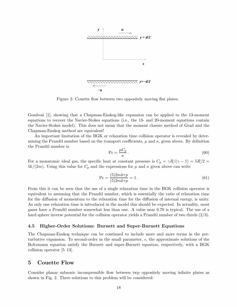
Figure 2: Couette flow between two oppositely moving flat plates.
Gombosi [1], showing that a Chapman-Enskog-like expansion can be applied to the 13-momentequations to recover the Navier-Stokes equations (i.e., the 13- and 20-moment equations containthe Navier-Stokes model). This does not mean that the moment closure method of Grad and theChapman-Enskog method are equivalent!
An important limitation of the BGK or relaxation time collision operator is revealed by deter-mining the Prandtl number based on the transport coefficients, µ and κ, given above. By definitionthe Prandtl number is
Pr =µCp
κ. (60)
For a monatomic ideal gas, the specific heat at constant pressure is Cp = γR/(γ − 1) = 5R/2 =5k/(2m). Using this value for Cp and the expressions for µ and κ given above can write
Pr =(5)2mkτp
(5)2mkτp= 1 . (61)
From this it can be seen that the use of a single relaxation time in the BGK collision operator isequivalent to assuming that the Prandtl number, which is essentially the ratio of relaxation timefor the diffusion of momentum to the relaxation time for the diffusion of internal energy, is unity.As only one relaxation time is introduced in the model this should be expected. In actuality, mostgases have a Prandtl number somewhat less than one. A value near 0.70 is typical. The use of ahard sphere inverse potential for the collision operator yields a Prandtl number of two thirds (2/3).
4.5 Higher-Order Solutions: Burnett and Super-Burnett Equations
The Chapman-Enskog technique can be continued to include more and more terms in the per-turbative expansion. To second-order in the small parameter, ǫ, the approximate solutions of theBoltzmann equation satisfy the Burnett and super-Burnett equation, respectively, with a BGKcollision operator [5–13].
5 Couette Flow
Consider planar subsonic incompressible flow between twp oppositely moving infinite plates asshown in Fig. 2. Three solutions to this problem will be considered:
18
i) the Navier-Stokes (continuum flow) solution,
ii) a kinetic (free-molecular flow) solution,
iii) and a slip flow solution based on the mean free path method.
The solution due to Lees [14] is also considered. A summary of the couette flow solution in eachcase now follows:
5.1 Navier-Stokes (Continuum Flow) Solution
u(y) = u◦
y
d, (62)
τxy = τwall = µu◦
d, (63)
and
2u(y = d/2)
u◦
= 1 , (64)
τwall
12ρu◦
√
2kT◦
πm
= 2Kn , (65)
where Kn = λ/d and µ = 12ρλv = 1
2ρλ√
(8kT◦)/(πm).
5.2 Kinetic (Free-Molecular Flow) Solution
Assuming full a accommodation:u(y) = 0 , (66)
τxy = τwall =1
2ρu◦
√
2kT◦
πm, (67)
and
2u(y = d/2)
u◦
= 0 , (68)
τwall
12ρu◦
√
2kT◦
πm
= 1 , (69)
5.3 Slip Flow Solution
Assuming full a accommodation (σ′ = 1):
u(y) = u◦
y
d
(
1
1 + 43
λd
)
, (70)
τxy = τwall = µu◦
d
(
1
1 + 43
λd
)
, (71)
and
2u(y = d/2)
u◦
=1
1 + 43Kn
, (72)
τwall
12ρu◦
√
2kT◦
πm
=2Kn
1 + 43Kn
, (73)
19
0.01
0.1
1
0.001 0.01 0.1 1 10 100
2 u
(y=
d/2)
/ u0
Kn = l/d
Navier-StokesFree-molecular flow
Slip flow (Mean Free Path)Lees solution (1959)
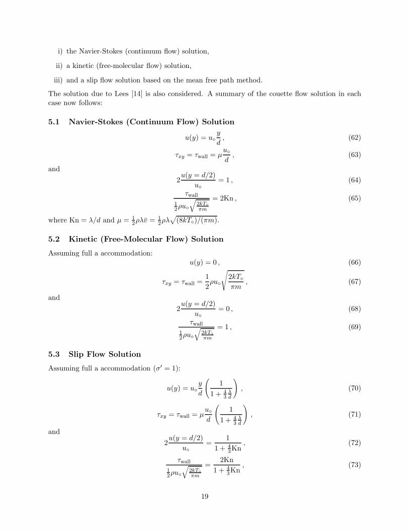
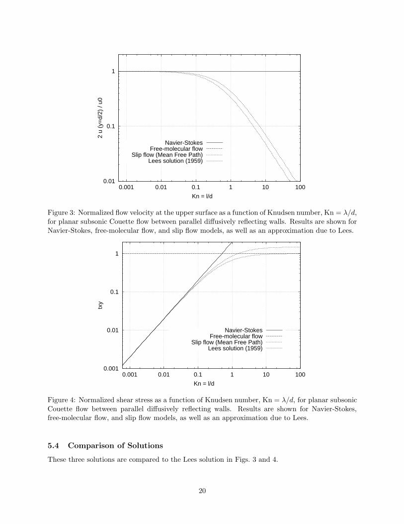
Figure 3: Normalized flow velocity at the upper surface as a function of Knudsen number, Kn = λ/d,for planar subsonic Couette flow between parallel diffusively reflecting walls. Results are shown forNavier-Stokes, free-molecular flow, and slip flow models, as well as an approximation due to Lees.
0.001
0.01
0.1
1
0.001 0.01 0.1 1 10 100
txy
Kn = l/d
Navier-StokesFree-molecular flow
Slip flow (Mean Free Path)Lees solution (1959)
Figure 4: Normalized shear stress as a function of Knudsen number, Kn = λ/d, for planar subsonicCouette flow between parallel diffusively reflecting walls. Results are shown for Navier-Stokes,free-molecular flow, and slip flow models, as well as an approximation due to Lees.
5.4 Comparison of Solutions
These three solutions are compared to the Lees solution in Figs. 3 and 4.
20
6 Shock-Wave Structure
6.1 Background
The application of several moment closures to the prediction of planar shock structure for amonatomic gas is considered. Shock profile prediction is a challenging problem that features sig-nificant departures from LTE, yet it is unencumbered with difficulties associated with complexgeometries and/or boundary condition prescription. For these reasons it is useful for evaluatingthe capabilities of moment methods. Included in the investigation are results for the 13- and 20-moment closures of Grad [15], which are based on expansions about a local Maxwellian, the 20-and 35-moment Gaussian-based closures recently proposed by Groth et al. [16, 17], and the 10-moment Gaussian closure considered in other recent studies by Brown et al. [18] and Levermoreand Morokoff [19], theoretical descriptions for all of which are provided for the case of planar one-dimensional flow. A higher-order point-implicit upwind finite-volume scheme, based on a MUSCL-type solution reconstruction procedure is used to solve the hyperbolic equation sets resulting fromthe closures and the predicted shock structures of the moment models are compared to those ofthe Navier-Stokes and Burnett equation, as well as DSMC calculations.
6.2 Moment Closures for One-Dimensional Planar Flows
In classical kinetic theory, the state of a dilute gas is prescribed by a distribution function for theparticle velocities, F , whose time evolution in phase space is governed by the Boltzmann equation.Neglecting external forces, the Boltzmann equation for a simple monatomic gas can be formulatedin terms of the components of the particle velocity vi, position coordinates xi, and time t andwritten as
∂F
∂t+ vi
∂F
∂xi=
δF
δt, (74)
where δF/δt is the Boltzmann collision operator representing the time rate of change of the distribu-tion function produced by inter-particle collisions. Refer to the texts by Chapman and Cowling [20]and Gombosi [1] for further details. A recent mathematical treatment of kinetic theory and theBoltzmann equation is given by Cercignani et al. [21].
In standard perturbative moment closure techniques (the non-perturbative closures recentlyproposed by Levermore [22] will not be considered here), the complex problem of directly solvingthe Boltzmann equation in six-dimensional phase space is avoided and replaced with one of solvinga system of generalized transport equations for various fluid quantities. Such a simplification isachieved by assuming that the distribution function can be approximated by a series expansion ofthe form
F = W [ 1 + A + Bα cα + Cαβ cαcβ + Dαβγ cαcβcγ
+ Eαβγδ cαcβcγcδ + · · · ] , (75)
where W is the weight function for the expansion, ci = vi − ui is the random particle velocity, andui is the average or bulk velocity of the particles. The expansion coefficients A, Bα, Cαβ, Dαβγ ,and Eαβγδ, etc..., are in general taken to functions of the velocity moments of F having the form
σ =
∫
∞
−∞
mMF (cα, xα, t)d3c = m < MF > , (76)
where M = M(c) and m is the particle mass. For M = 1, σ = ρ, where ρ is the mass density.Other higher-order velocity moments up to 5th-order can be defined as follows:
Pij = m < cicjF > , (77)
21
Qijk = m < cicjckF > , (78)
Kijkl = m < cicjckclF >
−1
ρ[PijPkl + PikPjl + PilPjk] , (79)
Sijklm = m < cicjckclcmF > , (80)
where Pij is the symmetric generalized pressure tensor, Qijk is the generalized heat flow tensor,and the fourth- and fifth-order tensors Rijkl and Sijklm represent the deviatoric components of thefourth- and fifth-order velocity moments, respectively. The hydrodynamic pressure, p, is related tothe pressure tensor by the expression p = Pii/3 and the usual fluid-dynamic or deviatoric stresstensor, τij , is given by τij = pδij − Pij . The heat flux vector, hi, is related to a simple contractionof the heat flow tensor and given by hi = Qijj/2. The infinte series of Eq. (75) is truncated byadopting an appropriate closing approximation and the time evolution of the resulting finite setof velocity moments, and hence expansion coefficients, are determined by solving a set of momentequations. Non-equilibrium solutions to the Boltzmann equation can then be constructed from thesolutions of the moment equations using the truncated series expansion relating the approximatedistribution function to the predicted velocity moments.
As noted in the introduction, the system of partial-differential equations (PDEs) describingthe transport of various velocity moments that results from the application of a moment closureare quasi-linear and hyperbolic. They also contain source terms representing inter-particle colli-sional (relaxation) processes. These hyperbolic systems may be expressed in the following weakconservation form:
∂U(N)
∂t+ ∇x ·F(N)
= S(N) , (81)
where U(N) is the solution vector of conserved velocity moments, F(N)
is a tensor representing themoment fluxes, and S(N) is the source vector describing the time rate of change of the velocitymoments produced by collisional processes. The integer N has been introduced to indicate thenumber of dependent variables associated with the full three-dimensional form of the closure model.
The specification of the source terms, S(N), necessitates the mathematical modeling of thecollision operator δF/δt. In the present numerical study, a two-scale relaxation-time approximationis adopted, as suggested by Levermore [22] and considered by Groth and Levermore [23]. In thissimplified model, complicated integral expressions for the collision operator are replaced by
δF
δt= −F −M
τ− (Pr − 1)
F − Gτ
, (82)
where τ is a characteristic relaxation time for the collision processes, Pr is the Prandtl number,and M and G are local Maxwellian and Gaussian distribution functions, respectively, given by
M =ρ
m (2πp/ρ)3/2exp
(
−1
2
ρc2
p
)
, (83)
G =ρ
m(2π)3/2∆1/2exp
(
−1
2Θ−1
αβcαcβ
)
. (84)
The characteristic relaxation time, which is the inverse of the collision frequency, ν = 1/τ , canbe related to the dynamic viscosity, µ, by means of the relationship τ = µ/p. The symmetrictensor, Θij, is related to the pressure tensor by the expression Θij = Pij/ρ and ∆ = detΘ. The
22
Maxwellian, M, corresponds to the form for solutions of the Boltzmann equation under conditionsof LTE (i.e., δF/δt = 0). The Gaussian distribution, G, is a form for non-equilibrium solutionsof the Boltzmann equation first deduced by Maxwell [24] and then re-discovered, or at least re-considered, many years later by Schluter [25] and then again by Holway [26]. It is a generalizationof the Maxwellian that accounts for the influences of non-zero fluid stresses in a non-perturbativemanner. Mathematical properties of the Gaussian are discussed by Levermore [22] and Groth et
al. [16].The collision operator of Eq. (82) is a two-time-scale extension of the BGK collision operator [2]
that preserves the usual collisional invariants and, under equilibrium conditions, δF/δt = 0 andF = M as required. The model also permits the formal recovery of a physically correct Navier-Stokes limit for Prandtl numbers different from unity, provided the functional dependence of theviscosity coefficient is adequately modeled. For a monatomic gas, Pr = 2/3 and, in many cases,the viscosity can be taken to have a power-law dependence on the temperture, T , of the form
µ = µo(T/To)ω , (85)
where µo and To are reference values and the exponent ω depends on the form for the forcesgoverning inter-particle collisional processes (ω = 1 for Maxwell molecules). Although there areinaccuracies associated with relaxation-time approximations of this type, the model is thought tobe sufficient for the applications considered herein.
The remainder of this section will provide a brief summary of the moment closures consideredin the present study, for the particular case of planar one-dimensional flows in the x-direction of aCartesian coordinate system (x, y, z). Included in the summary are the Maxwellian and Gaussianclosures, Maxwellian-based 13- and 20-moment closures of Grad [15], and Gaussian-based 20- and35-moment models described by Groth et al. [16, 17]. In each case the approximate form for thedistribution function, moment equations, and closing relationship are discussed. Note that for theone-dimensional case, the moment equations of Eq. (81) reduce to
∂U(N)
∂t+
∂F(N)
∂x= S(N) , (86)
where F(N) is the conservative flux vector.
6.2.1 5-Moment Maxwellian Closure
The most elementary moment closure is the 5-moment Maxwellian model for which N = 5. In thisapproximation, it is assumed that the gas is everywhere in LTE and that the phase-space velocitydistribution function is given by the Maxwellian, M, which for one-dimensional planar flows hasthe form
M =ρ
m (2πp/ρ)3/2exp
[
−1
2
ρ(c2x + 2c2
y)
p
]
. (87)
The closing relationships implied by these assumptions are
τxx = 0 , hx = 0 , (88)
and the resulting hyperbolic set of moment equations are the well-known Euler equations of com-pressible gas dynamics that describe the evolution of ρ, u, and p. The solution vector, U(5), andsource vector, S(5), of the Euler equations for a monatomic non-reacting gas can be expressed as
U(5) =
ρρu
1
2ρu2 +
3
2p
, S(5) =
000
. (89)
23
According to this inviscid model, the propagation speed of acoustical disturbances is a =√
5p/3ρand strict hyperbolicity of the Euler equations is ensured for ρ > 0 and p > 0. Note that thediscontinuous solutions of shock wave structure provided by the Maxwellian closure are fully un-derstood and will not be considered herein. However, the Euler equations are used in the shockprofile computations for the the higher-order moment closures to prescribe initial and boundarydata and have therefore been briefly reviewed.
6.2.2 13-Moment Maxwellian-Based Closure
The 13- and 20-moment closures of Grad [15] offer estimates of non-equilibrium solutions to theBoltzmann equation that are implicitly based on perturbations to the equilibrium Maxwelliansolution. Both closures are based on a series expansion for F of the form given by Eq. (75) wherethe weight function is taken to be the Maxwellian (i.e., W = M). In the one-dimensional case, theapproximated form for the velocity distribution of the 13-moment model can be written as
F (13) = M[
1 − hx
ρa3x
cx
ax
+(Pxx − Pyy)
3ρa2x
(
c2x
a2x
−c2y
a2x
)
+hx
5ρa3x
cx
ax
(
c2x
a2x
+ 2c2y
a2x
)]
, (90)
where M is given by Eq. (87), ax =√
p/ρ, p = (Pxx + 2Pyy)/3, and closure has been achieved byassuming that
Qxxx =6
5hx , Qxyy =
2
5hx , (91)
Kxxxx = −3τ2xx
ρ, Kxxyy =
1
2
τ2xx
ρ, (92)
Kyyyy = −3
4
τ2xx
ρ, (93)
with τxx = −2(Pxx − Pyy)/3. For planar one-dimensional flows, there are five dependent variablesassociated with the 13-moment closure. The solution vector of the moment equations describingthe transport of ρ, u, Pxx, Pyy, and hx is
U(13) =
ρρu
ρu2 + Pxx
Pyy1
2ρu3 +
1
2u(3Pxx + 2Pyy) + hx
. (94)
24
The related source column vector, derived by evaluating the appropriate velocity moments of thetwo-scale relaxation-time model for the collision operator described above, is given by
S(13) =
0
0
− 2
3τ(Pxx − Pyy)
1
3τ(Pxx − Pyy)
− 2
3τu(Pxx − Pyy) −
Pr
τhx
. (95)
Note that, as with all moment closures, the 13-moment approximation has introduced additionaltransport equations beyond those appearing at the level of the Maxwellian for describing the higher-order velocity moments such as heat flux, hx. This is contrast to the Navier-Stokes and Burnettmodels which express these higher-order moment in terms of gradients of the lower-order quantities.
6.2.3 20-Moment Maxwellian-Based Closure
The primary difference between the 13- and 20-moment Grad closures is that, in the 20-momentmodel, the closing relationship for the heat flow tensor expressed in terms of the heat flux vector,which for the one-dimensional case is represented by the relations given in Eq. (91), are not utilizedand the full heat flow tensor is considered. The approximate form for the distribution function ofthe 20-moment closure is given by
F (20) = M[
1 −(
Qxxx
2ρa3x
+Qxyy
ρa3x
)
cx
ax
+(Pxx − Pyy)
3ρa2x
(
c2x
a2x
−c2y
a2x
)
+Qxxx
6ρa3x
c3x
a3x
+Qyyy
ρa3x
cx
ax
c2y
a2x
]
, (96)
and the solution and source vectors of the system of moment equations for the six dependentvariables ρ, u, Pxx, Pyy, Qxxx, and Qyyy may be written as
U(20) =
ρρu
ρu2 + Pxx
Pyy
ρu3 + 3uPxx + Qxxx
uPyy + Qxyy
, (97)
25
S(20) =
0
0
− 2
3τ(Pxx − Pyy)
1
3τ(Pxx − Pyy)
−2
τu(Pxx − Pyy) −
Pr
τQxxx
1
3τu(Pxx − Pyy) −
Pr
τQxyy
, (98)
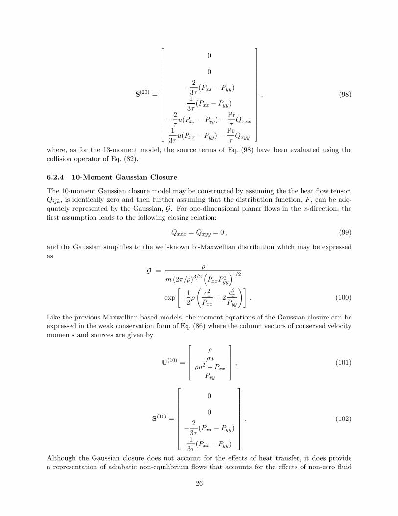
where, as for the 13-moment model, the source terms of Eq. (98) have been evaluated using thecollision operator of Eq. (82).
6.2.4 10-Moment Gaussian Closure
The 10-moment Gaussian closure model may be constructed by assuming the the heat flow tensor,Qijk, is identically zero and then further assuming that the distribution function, F , can be ade-quately represented by the Gaussian, G. For one-dimensional planar flows in the x-direction, thefirst assumption leads to the following closing relation:
Qxxx = Qxyy = 0 , (99)
and the Gaussian simplifies to the well-known bi-Maxwellian distribution which may be expressedas
G =ρ
m (2π/ρ)3/2(
PxxP 2yy
)1/2
exp
[
−1
2ρ
(
c2x
Pxx+ 2
c2y
Pyy
)]
. (100)
Like the previous Maxwellian-based models, the moment equations of the Gaussian closure can beexpressed in the weak conservation form of Eq. (86) where the column vectors of conserved velocitymoments and sources are given by
U(10) =
ρρu
ρu2 + Pxx
Pyy
, (101)
S(10) =
0
0
− 2
3τ(Pxx − Pyy)
1
3τ(Pxx − Pyy)
. (102)
Although the Gaussian closure does not account for the effects of heat transfer, it does providea representation of adiabatic non-equilibrium flows that accounts for the effects of non-zero fluid
26
stresses in a non-perturbative manner (i.e., unlike the expansions for the velocity distribution ofthe 13- and 20-moment closure, differences in the components of the pressure Pxx and Pyy areaccounted for directly in the argument of the exponential of Eq. (100) such that G remains positivefor all physically realistic values of Pij). It can also be shown that the one-dimensional form of themoment equations of the Gaussian model remain strictly hyperbolic for ρ > 0 and Pxx > 0. Theseand other more detailed mathematical and solution properties of the Gaussian closure have beenexplored in several recent studies [16,18,19,22]. Refer to these references for further details.
6.2.5 20-Moment Gaussian-Based Closure
An alternate hierarchy of higher-order closure models to the Maxwellian-based heirarchy consideredby Grad can be constructed by using the Gaussian as a weight function in place of the usualMaxwellian. Gassian-based closures of this type have been recently considered by Groth et al.
[16, 27]. At the 20-moment level, the one-dimensional form for the approximate particle velocitydistribution function is
F (20) = G[
1 −(
Qxxx
2ρa3x
+Qxyy
ρa3x
Pxx
Pyy
)
cx
ax
+Qxxx
6ρa3x
c3x
a3x
+Qxyy
ρa3x
P 2xx
P 2yy
cx
ax
c2y
a2x
]
, (103)
where ax =√
Pxx/ρ and closure is provided by assuming that the deviatoric components of thefourth-order velocity moments vanish. The latter implies that
Kxxxx = Kxxyy = Kyyyy = 0 , (104)
in the one-dimensional case. The solution and source column vectors for the system of momentequations that results from this 20-moment Gaussian-based approximation are identical to thoseof the 20-moment Maxwellian-based closure given in Eqs. (97) and (98); the differences in the twoquasi-linear equations sets appear in the moment flux vectors (not shown here). In comparison tothe Grad Maxwellian-based model, an important advantage of the Gaussian-based approximationis that the influences of the fluid stresses are incorporated directly in the weight function of theexpansion, W = G, and, as such, the approximate form for the distribution function should remainvalid for a larger range of flow conditions. It can also be shown that the eigenstructure of the 20-moment Gaussian-based model has a much simpler mathematical form than that of the Maxwellian-based model, making the Gaussian-based model more amenable to solution by numerical methods.It should also be mentioned that the Gaussian-based 20-moment model has similarities with thebi-Maxwellian-based 16-moment closure considered in the studies of Oraevskii et al. [25], Choduraand Pohl [28], Demars and Schunk [29], and Barakat and Schunk [30]. In fact, for planar one-dimensional flows, the two closures are identical in every respect.
6.2.6 35-Moment Gaussian-Based Closure
A Gaussian-based 35-moment closure that accounts for variations in the deviatoric componentsof the fourth-order velocity moments can be constructed by closing at the level of the fifth-ordervelocity moments. Such a model was recently proposed and investigated in considerable detail byGroth et al. [16] and has been shown to possess several desirable mathematical properties. Forone-dimensional planar flows, the closing relations relating the fifth-order velocity moments to the
27
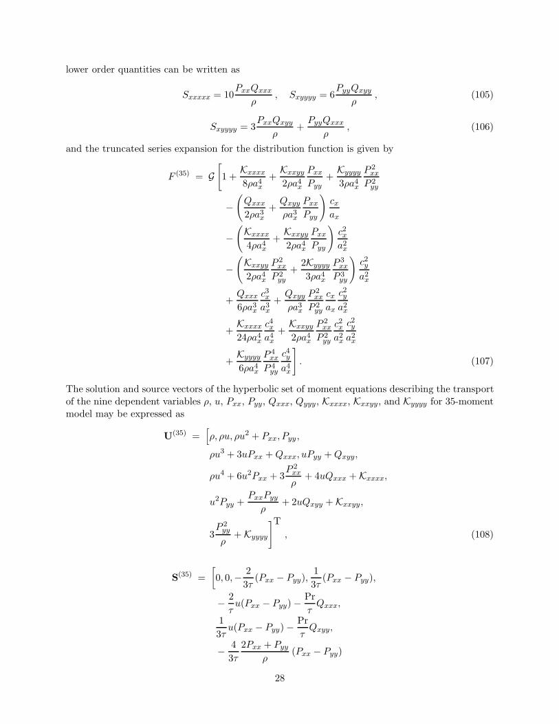
lower order quantities can be written as
Sxxxxx = 10PxxQxxx
ρ, Sxyyyy = 6
PyyQxyy
ρ, (105)
Sxyyyy = 3PxxQxyy
ρ+
PyyQxxx
ρ, (106)
and the truncated series expansion for the distribution function is given by
F (35) = G[
1 +Kxxxx
8ρa4x
+Kxxyy
2ρa4x
Pxx
Pyy+
Kyyyy
3ρa4x
P 2xx
P 2yy
−(
Qxxx
2ρa3x
+Qxyy
ρa3x
Pxx
Pyy
)
cx
ax
−(
Kxxxx
4ρa4x
+Kxxyy
2ρa4x
Pxx
Pyy
)
c2x
a2x
−(
Kxxyy
2ρa4x
P 2xx
P 2yy
+2Kyyyy
3ρa4x
P 3xx
P 3yy
)
c2y
a2x
+Qxxx
6ρa3x
c3x
a3x
+Qxyy
ρa3x
P 2xx
P 2yy
cx
ax
c2y
a2x
+Kxxxx
24ρa4x
c4x
a4x
+Kxxyy
2ρa4x
P 2xx
P 2yy
c2x
a2x
c2y
a2x
+Kyyyy
6ρa4x
P 4xx
P 4yy
c4y
a4x
]
. (107)
The solution and source vectors of the hyperbolic set of moment equations describing the transportof the nine dependent variables ρ, u, Pxx, Pyy, Qxxx, Qyyy, Kxxxx, Kxxyy, and Kyyyy for 35-momentmodel may be expressed as
U(35) =[
ρ, ρu, ρu2 + Pxx, Pyy ,
ρu3 + 3uPxx + Qxxx, uPyy + Qxyy,
ρu4 + 6u2Pxx + 3P 2
xx
ρ+ 4uQxxx + Kxxxx,
u2Pyy +PxxPyy
ρ+ 2uQxyy + Kxxyy,
3P 2
yy
ρ+ Kyyyy
]T
, (108)
S(35) =
[
0, 0,− 2
3τ(Pxx − Pyy),
1
3τ(Pxx − Pyy),
− 2
τu(Pxx − Pyy) −
Pr
τQxxx,
1
3τu(Pxx − Pyy) −
Pr
τQxyy,
− 4
3τ
2Pxx + Pyy
ρ(Pxx − Pyy)
28
− 4
τu2(Pxx − Pyy) −
4Pr
τuQxxx
− Pr
τKxxxx,
1
9τ
Pxx − 4Pyy
ρ(Pxx − Pyy)
+1
3τu2(Pxx − Pyy) −
2Pr
τuQxyy
− Pr
τKxxyy,
1
3τ
Pxx + 5Pyy
ρ(Pxx − Pyy)
− Pr
τKyyyy
]T. (109)
Refer to [16,17] for discussions of the hyperbolicity, eigenstructure, and dispersive-wave propertiesof the 35-moment equations.
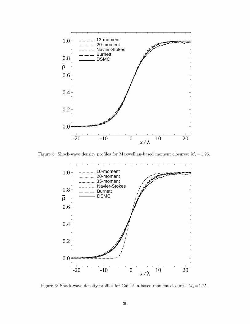
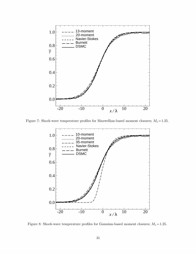
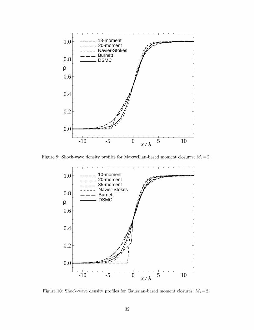
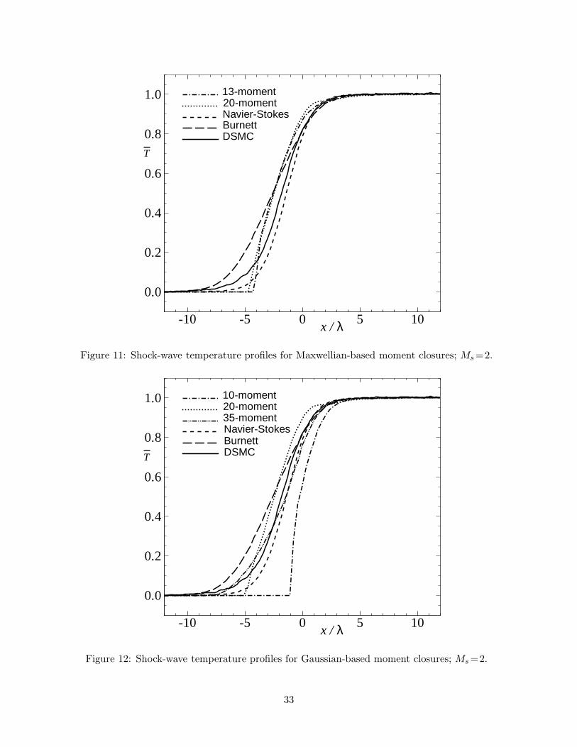
6.3 Predicted Shock Structure
The predicted shock structures of the various moment closures described in the preceding sectionsare now compared for a monatomic gas. In all cases considered, the gas is assumed to be a Maxwellgas with Pr = 2/3 and having a coefficient of viscosity, µ, that is linearly dependent on temperature(i.e., ω = 1).
29
-20 -10 0 10 20
0.0
0.2
0.4
0.6
0.8
1.0
−ρDSMCBurnettNavier-Stokes20-moment13-moment
x / λ
Figure 5: Shock-wave density profiles for Maxwellian-based moment closures; Ms =1.25.
-20 -10 0 10 20
0.0
0.2
0.4
0.6
0.8
1.0
−ρ DSMCBurnettNavier-Stokes
10-moment20-moment35-moment
x / λ
Figure 6: Shock-wave density profiles for Gaussian-based moment closures; Ms =1.25.
30
-20 -10 0 10 20
0.0
0.2
0.4
0.6
0.8
1.0
−DSMCBurnettNavier-Stokes20-moment13-moment
T
x / λ
Figure 7: Shock-wave temperature profiles for Maxwellian-based moment closures; Ms =1.25.
-20 -10 0 10 20
0.0
0.2
0.4
0.6
0.8
1.0
− DSMCBurnettNavier-Stokes
10-moment20-moment35-moment
T
x / λ
Figure 8: Shock-wave temperature profiles for Gaussian-based moment closures; Ms =1.25.
31
-10 -5 0 5 10
0.0
0.2
0.4
0.6
0.8
1.0
−ρ
x / λ
DSMCBurnettNavier-Stokes20-moment13-moment
Figure 9: Shock-wave density profiles for Maxwellian-based moment closures; Ms =2.
-10 -5 0 5 10
0.0
0.2
0.4
0.6
0.8
1.0
−ρ
x / λ
DSMCBurnettNavier-Stokes
10-moment20-moment35-moment
Figure 10: Shock-wave density profiles for Gaussian-based moment closures; Ms =2.
32
-10 -5 0 5 10
0.0
0.2
0.4
0.6
0.8
1.0
−
x / λ
DSMCBurnettNavier-Stokes20-moment13-moment
T
Figure 11: Shock-wave temperature profiles for Maxwellian-based moment closures; Ms =2.
-10 -5 0 5 10
0.0
0.2
0.4
0.6
0.8
1.0
−
x / λ
DSMCBurnettNavier-Stokes
10-moment20-moment35-moment
T
Figure 12: Shock-wave temperature profiles for Gaussian-based moment closures; Ms =2.
33
Appendices
A Velocity Moments of the Maxwellian Distribution Function
A.1 Random-Velocity Moments
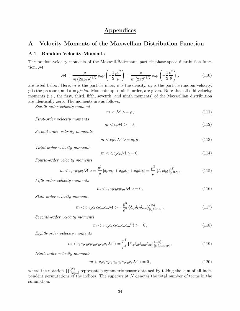
The random-velocity moments of the Maxwell-Boltzmann particle phase-space distribution func-tion, M,
M =ρ
m (2πp/ρ)3/2exp
(
−1
2
ρc2
p
)
=ρ
m (2πθ)3/2exp
(
−1
2
c2
θ
)
, (110)
are listed below. Here, m is the particle mass, ρ is the density, cα is the particle random velocity,p is the pressure, and θ = p/rho. Moments up to ninth order, are given. Note that all odd velocitymoments (i.e., the first, third, fifth, seventh, and ninth moments) of the Maxwellian distributionare identically zero. The moments are as follows:
Zeroth-order velocity moment
m < M >= ρ , (111)
First-order velocity moments
m < ciM >= 0 , (112)
Second-order velocity moments
m < cicjM >= δijp , (113)
Third-order velocity moments
m < cicjckM >= 0 , (114)
Fourth-order velocity moments
m < cicjckclM >=p2
ρ[δijδkl + δikδjl + δilδjk] =
p2
ρ{δijδkl}(3)
[ijkl] , (115)
Fifth-order velocity moments
m < cicjckclcmM >= 0 , (116)
Sixth-order velocity moments
m < cicjckclcmcnM >=p3
ρ2{δijδklδmn}(15)
[ijklmn] , (117)
Seventh-order velocity moments
m < cicjckclcmcncoM >= 0 , (118)
Eighth-order velocity moments
m < cicjckclcmcncocpM >=p4
ρ3{δijδklδmnδop}(105)
[ijklmnop] , (119)
Ninth-order velocity moments
m < cicjckclcmcncocpcqM >= 0 , (120)
where the notation {}(N)[ijk...] represents a symmetric tensor obtained by taking the sum of all inde-
pendent permutations of the indices. The superscript N denotes the total number of terms in thesummation.
34
A.2 Contracted Random-Velocity Moments
Simple index contraction of the preceding moments is possible. The following contracted quantitiesof the the Maxwellian distribution function are useful:
Contracted second-order velocity moments
m < c2M >= 3p , (121)
Contracted fourth-order velocity moments
m < cicjc2M >= 5
p2
ρδij , (122)
m < c4M >= 15p2
ρ, (123)
Contracted sixth-order velocity moments
m < cicjckclc2M >= 7
p3
ρ2[δijδkl + δikδjl + δilδjk] = 7
p3
ρ2{δijδkl}(3)
[ijkl] , (124)
m < cicjc4M >= 35
p3
ρ2δij , (125)
m < c6M >= 105p3
ρ2. (126)
References
[1] Gombosi, T. I., Gaskinetic Theory , Cambridge University Press, Cambridge, 1994.
[2] Bhatnagar, P. L., Gross, E. P., and Krook, M., “A Model for Collision Processes in Gases. I.Small Amplitude Processes in Charged and Neutral One-Component Systems,” Physical Rev.,Vol. 94, No. 3, 1954, pp. 511–525.
[3] Chapman, S., “On the Kinetic Theory of a Gas. Part II. – A Composite Monoatomic Gas:Diffusion, Viscosity, and Thermal Conduction,” Phil. Trans. Royal Soc. London A, Vol. 217,1916, pp. 115–116.
[4] Enskog, D., Kinetishe Theorie der Vorgange in Massing Verdumten Gasen, Ph.D. thesis, Uni-versity of Upsala, 1917.
[5] Burnett, D., “The Distribution of Velocities in a Slightly Non-Uniform Gas,” Proc. London
Math. Soc., Vol. 39, 1935, pp. 385–430.
[6] Burnett, D., “The Distribution of Molecular Velocities and the Mean Motion in a Non-UniformGas,” Proc. London Math. Soc., Vol. 40, 1935, pp. 382–435.
[7] Bobylev, A. V., “The Chapman-Enskog and Grad Methods for Solving the Boltzmann Equa-tion,” Sov. Phys. Dokl., Vol. 27, No. 1, 1982, pp. 29–31.
[8] Woods, L. C., “Frame-Indifferent Kinetic Theory,” J. Fluid Mech., Vol. 136, 1983, pp. 423–433.
35
[9] Zhong, X., MacCormack, R. W., and Chapman, D. R., “Evaluation of Slip Boundary Condi-tions for the Burnett Equations with Application to Hypersonic Leading Edge Flow,” Proceed-
ings of the Fourth International Symposium on Computational Fluid Dynamics, University of
California, Davis, California, September 9–12, 1991 , Vol. II, University of California, Davis,California, U.S.A., 1991, pp. 1360–1366.
[10] Zhong, X., MacCormack, R. W., and Chapman, D. R., “Stabilization of the Burnett Equationsand Application to Hypersonic Flows,” AIAA J., Vol. 31, No. 6, 1993, pp. 1036–1043.
[11] Reese, J. M., Woods, L. C., Thivet, F. J. P., and Candel, S. M., “A Second-Order Descriptionof Shock Structure,” J. Comput. Phys., Vol. 117, 1995, pp. 240–250.
[12] Comeaux, K. A., Chapman, D. R., and MacCormack, R. W., “An Analysis of the BurnettEquations Based on the Second Law of Thermodynamics,” Paper 95-0415, AIAA, January1995.
[13] Balakrishnan, R. and Agarwal, R. K., “A Kinetic Theory Based Scheme for the NumericalSolution of the BGK-Burnett Equations for Hypersonic Flows in the Continuum-TransitionRegime,” Paper 96-0602, AIAA, January 1996.
[14] Vincenti, W. G. and Kruger, C. H., Introduction to Physical Gas Dynamics, R. E. KriegerPublishing, Huntington, NY, 1975.
[15] Grad, H., “On the Kinetic Theory of Rarefied Gases,” Commun. Pure Appl. Math., Vol. 2,1949, pp. 331–407.
[16] Groth, C. P. T., Gombosi, T. I., Roe, P. L., and Brown, S. L., “A Gaussian-Based Closurefor Rarefied Gases: Derivation, Moment Equations, and Wave Structure,” submitted to theJournal of Fluid Mechanics, September 1998.
[17] Groth, C. P. T., Roe, P. L., Gombosi, T. I., and Brown, S. L., “On the Nonstationary WaveStructure of a 35-Moment Closure for Rarefied Gas Dynamics,” Paper 95-2312, AIAA, June1995.
[18] Brown, S. L., Roe, P. L., and Groth, C. P. T., “Numerical Solution of a 10-Moment Model forNonequilibrium Gasdynamics,” Paper 95-1677, AIAA, June 1995.
[19] Levermore, C. D. and Morokoff, W. J., “The Gaussian Moment Closure for Gas Dynamics,”submitted to the SIAM Journal on Applied Analysis, February 1996.
[20] Chapman, S. and Cowling, T. G., The Mathematical Theory of Non-Uniform Gases, Cam-bridge University Press, Cambridge, 1960.
[21] Cercignani, C., Illner, R., and Pulvirenti, M., The Mathematical Theory of Dilute Gases,Springer-Verlag, New York, 1994.
[22] Levermore, C. D., “Moment Closure Hierarchies for Kinetic Theories,” J. Stat. Phys., Vol. 83,1996, pp. 1021–1065.
[23] Groth, C. P. T. and Levermore, C. D., “Beyond the Navier-Stokes Approximation: TransportCorrections to the Gaussian Closure,” in preparation, May 1996.
[24] Maxwell, J. C., “On the Dynamical Theory of Gases,” Philosophical Transactions of the Royal
Society of London, Vol. 157, 1867, pp. 49–88.
36
[25] Oraevskii, V., Chodura, R., and Feneberg, W., “Hydrodynamic Equations for Plasmas inStrong Magnetic Fields — I Collisionless Approximation,” Plasma Phys., Vol. 10, 1968,pp. 819–828.
[26] Holway, L. H., Approximation Procedures for Kinetic Theory , Ph.D. thesis, Harvard University,1963.
[27] Groth, C. P. T., Gombosi, T. I., Roe, P. L., and Brown, S. L., “Gaussian-Based Moment-Method Closures for the Solution of the Boltzmann Equation,” Proceedings of the Fifth Inter-
national Conference on Hyperbolic Problems — Theory, Numerics, Applications, University
of New York at Stony Brook, Stony Brook, New York, U.S.A., June 13–17, 1994 , edited byJ. Glimm, M. J. Graham, J. W. Grove, and B. J. Plohr, World Scientific, New Jersey, 1996,pp. 339–346.
[28] Chodura, R. and Pohl, F., “Hydrodynamic Equations for Plasmas in Strong Magnetic Fields— II Transport Equations Including Collisions,” Plasma Phys., Vol. 13, 1971, pp. 645–658.
[29] Demars, H. G. and Schunk, R. W., “Transport Equations for Multispecies Plasmas Based onIndividual Bi-Maxwellian Distributions,” J. Phys. D: Appl. Phys., Vol. 12, 1979, pp. 1051–1077.
[30] Barakat, A. R. and Schunk, R. W., “Comparison of Transport Equations Based on Maxwellianand Bi-Maxwellian Distributions for Anisotropic Plasmas,” J. Phys. D: Appl. Phys., Vol. 15,1982, pp. 1195–1216.
37