Embed Size (px)
Citation preview
EXPERIMENT #2
Rectilinear Control System
Introduction:
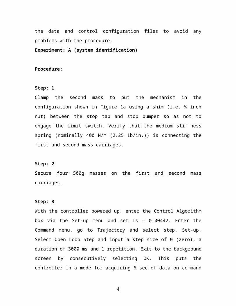
This classical plant is readily transformed into the variety of configuration shown below.
It serves to vividly demonstrate both lumped parameter dynamics and generic control
issues. This system appears commonly in dynamics and controls text books and serves as
a benchmark for control method evaluation. The mechanism features adjustable masses,
interchangeable springs and adjustable air damping. Its dynamic properties are generally
the rectilinear equivalent of those of the Torsional Apparatus with additional parameter
adjustment capability. As with Model 205, this system provides vivid demonstrations of
elementary topics such as rigid body PID control, lead/lag compensators, phase and gain
margin, trajectory tracking, and regulation-as well as advanced high order collocated and
noncollocated system control. The two apparatuses also clearly demonstrate salient
properties of flexible systems such as mode shapes, natural frequencies, and
characteristic transient and frequency responses. An optional secondary drive may be
positioned at any output (mass carriage) to create a MIMO plant and provide for the
study of disturbance rejection.
1
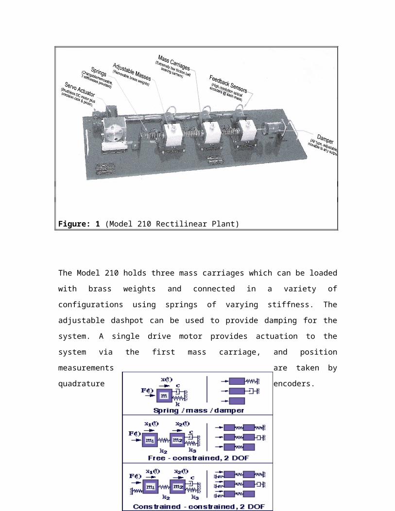
Figure: 1 (Model 210 Rectilinear Plant)
The Model 210 holds three mass carriages which can be loaded with brass weights and
connected in a variety of configurations using springs of varying stiffness. The adjustable
dashpot can be used to provide damping for the system. A single drive motor provides
actuation to the system via the first mass carriage, and position measurements are taken
by quadrature encoders.
This report was made with the help of other students and with the help of my supervisor
and it is basic of rectilinear control system plant identification (model 210). This report is
related to those of (Torsional system). The equations and the procedure are the same way
but now we have a mass than disk. The purpose of this report is to identify the plant
parameters, implement a variety of control schemes, and demonstrate many important
control principles. This report includes experiments, which will be executed, analyzed
and also mathematical equations. The user to be done this experiments must be familiar
with the (model 210), how is work and to read or remember from the last years about
2

control systems to have the ability to solve the equations. The model to be work needs
I/O electronic unit connected with a computer that is able to show the data and the
waveform from each encoder. Finally the user must save the data and control
configuration files to avoid any problems with the procedure.
Experiment: A (system identification)
Procedure:
Step: 1
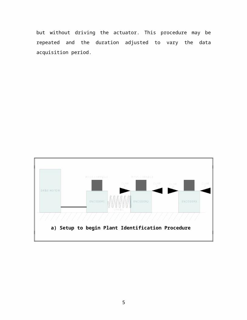
Clamp the second mass to put the mechanism in the configuration shown in Figure 1a
using a shim (i.e. ¼ inch nut) between the stop tab and stop bumper so as not to engage
the limit switch. Verify that the medium stiffness spring (nominally 400 N/m (2.25
1b/in.)) is connecting the first and second mass carriages.
Step: 2
Secure four 500g masses on the first and second mass carriages.
Step: 3
With the controller powered up, enter the Control Algorithm box via the Set-up menu and
set Ts = 0.00442. Enter the Command menu, go to Trajectory and select step, Set-up.
Select Open Loop Step and input a step size of 0 (zero), a duration of 3000 ms and 1
repetition. Exit to the background screen by consecutively selecting OK. This puts the
controller in a mode for acquiring 6 sec of data on command but without driving the
actuator. This procedure may be repeated and the duration adjusted to vary the data
acquisition period.
3
a) Setup to begin Plant Identification Procedure
b) Second Setup in Plant Identification Procedure
4
c) Third Setup in Plant Identification Procedure
Figure: 2 Configurations for Plant Identification
(model 210a. Four 500g weights on each active carriage.)
Step: 4
Go to Set up Data Acquisition in the Data menu and select Encoder # 1 and Encoder # 2
as data to acquire and specify data sampling every 2 (two) servo cycles (i.e. every 2 T s’s).
Select OK to exit. Select Zero Position from the Utility menu to zero the encoder
positions.
Step: 5
Select Execute from the Command menu. Prepare to manually displace the first mass
carriage approximately 2.5 cm. Exercise caution in displacing the carriage so as not to
engage the travel limit switch. With the first mass displaced approximately 2.5 cm in
either direction, select Run from the Execute box and release the mass approximately 1
second later. The mass will oscillate and attenuate while encoder data is collected to
record this response. Select OK after data is uploaded.
Step: 6
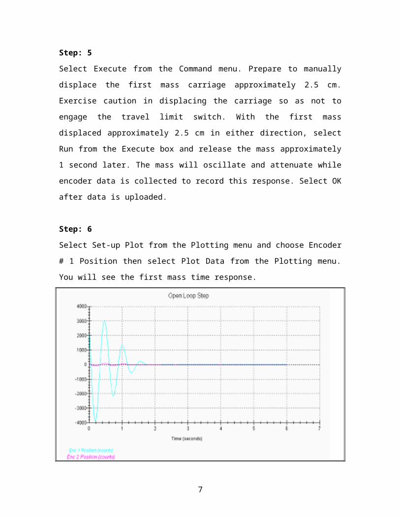
Select Set-up Plot from the Plotting menu and choose Encoder # 1 Position then select
Plot Data from the Plotting menu. You will see the first mass time response.
5
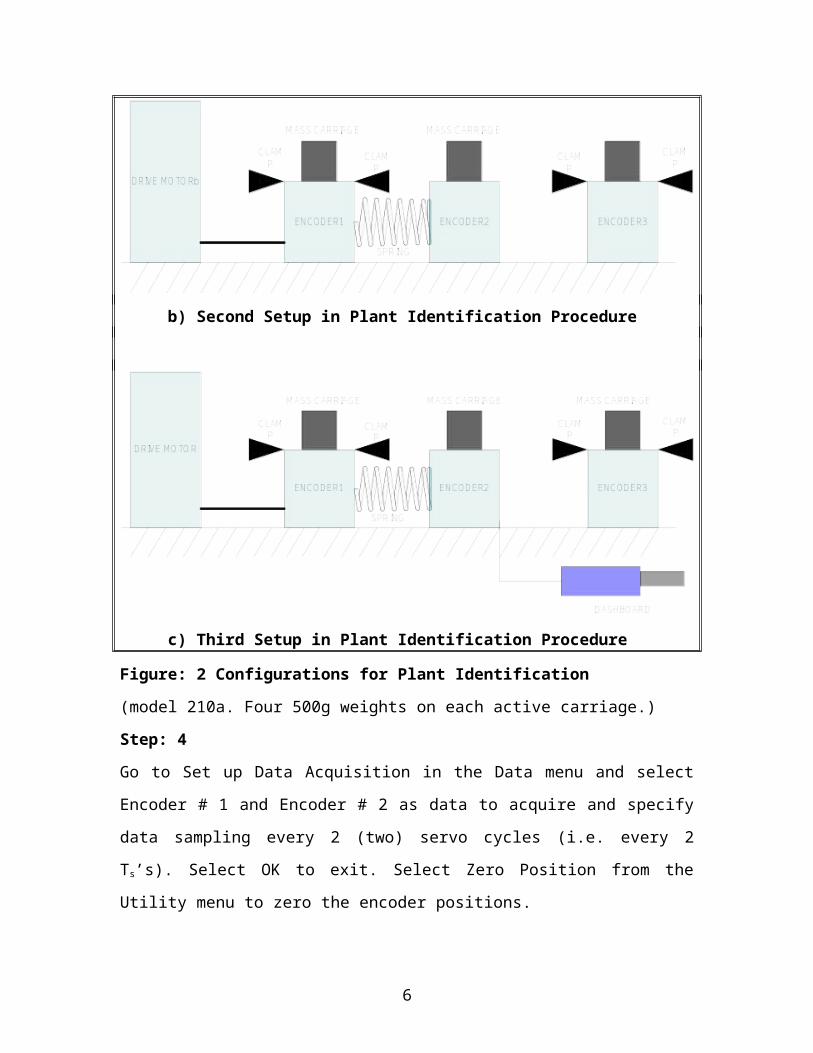
Figure: 3 (encoder # 1 & # 2 loaded)
Step: 7
Choose several consecutive cycles (say ~5) in the amplitude range between 5500 and
1000 counts (this is representative of oscillation amplitudes during later closed loop
control maneuvers. Much smaller amplitude responses become dominated by nonlinear
friction effects and do not reflect the salient system dynamics).
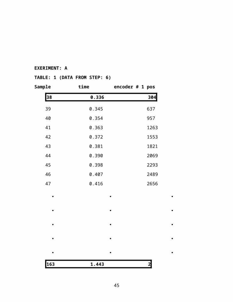
We choose,
t1 = 0.336 seconds 304 counts from TABLE 1
t2 = 1.443 seconds 2 counts from TABLE 1
so the number of the cycles between t1 and t2 is n = 2 cycles
Divide the number of cycles by the time taken to complete them being sure to take
beginning and end times from the same phase of the respective cycles.
f = n/(t2-t1) f =frequency (Hz)
6
f = 2/(1.443-0.336)
f = 1.806 Hz
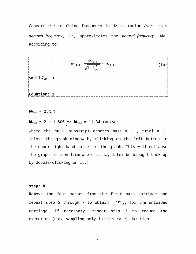
Convert the resulting frequency in Hz to radians/sec. this damped frequency, ωd,
approximates the natural frequency, ωn, according to:
(for small )
Equation: 1
ωnm11 = 2.π.f
ωnm11 = 2.π.1.806 => ωnm11 = 11.34 rad/sec
where the “m11” subscript denotes mass # 1 , trial # 1. (close the graph window by
clicking on the left button in the upper right hand corner of the graph. This will collapse
the graph to icon from where it may later be brought back up by double-clicking on it.)
step: 8
Remove the four masses from the first mass carriage and repeat step 5 through 7 to obtain
for the unloaded carriage. If necessary, repeat step 3 to reduce the execution (data
sampling only in this case) duration.
7
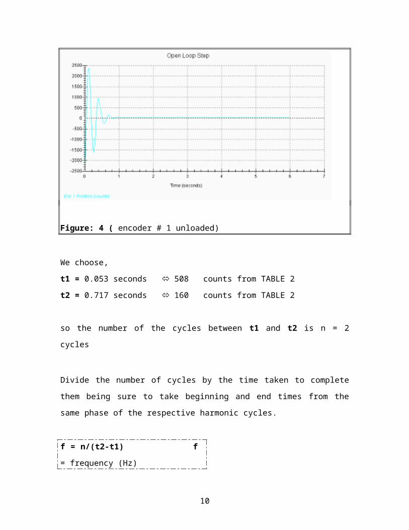
Figure: 4 ( encoder # 1 unloaded)
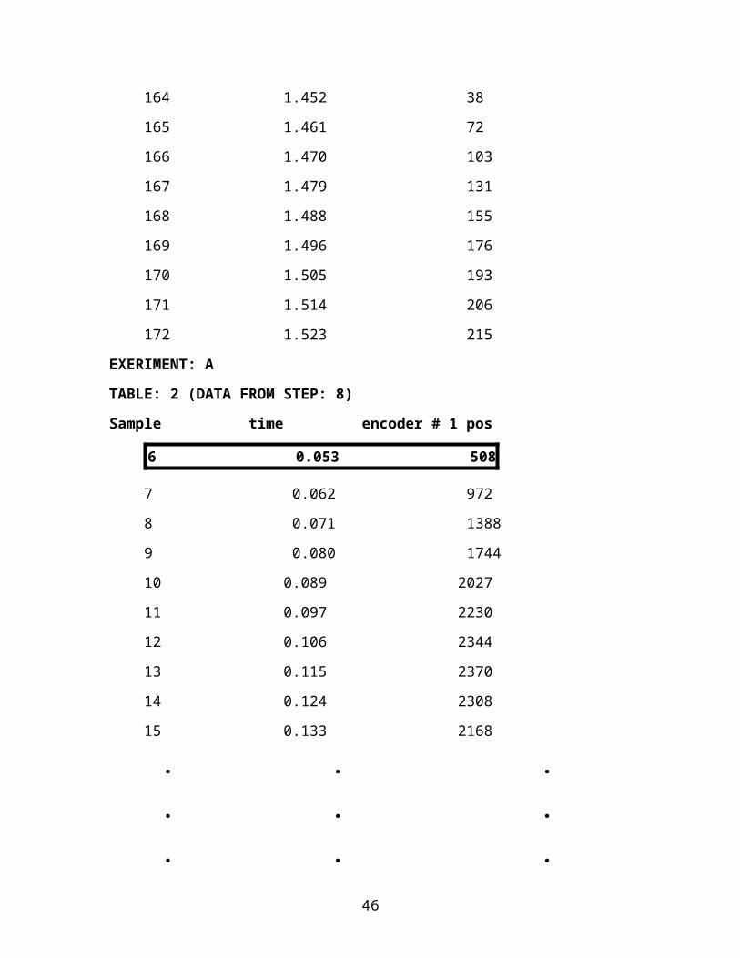
We choose,
t1 = 0.053 seconds 508 counts from TABLE 2
t2 = 0.717 seconds 160 counts from TABLE 2
so the number of the cycles between t1 and t2 is n = 2 cycles
Divide the number of cycles by the time taken to complete them being sure to take
beginning and end times from the same phase of the respective harmonic cycles.
f = n/(t2-t1) f = frequency (Hz)
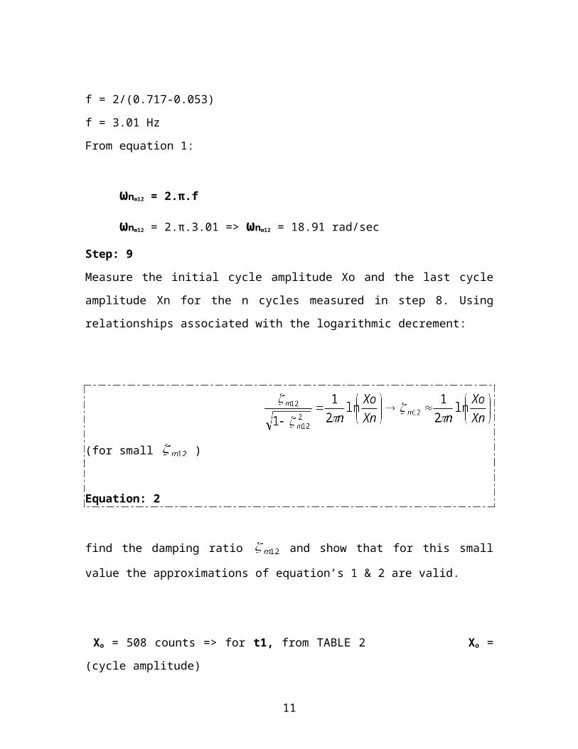
f = 2/(0.717-0.053)
f = 3.01 Hz
From equation 1:
ωnm12 = 2.π.f
ωnm12 = 2.π.3.01 => ωnm12 = 18.91 rad/sec
8
Step: 9
Measure the initial cycle amplitude Xo and the last cycle amplitude Xn for the n cycles
measured in step 8. Using relationships associated with the logarithmic decrement:
(for small )
Equation: 2
find the damping ratio and show that for this small value the approximations of
equation’s 1 & 2 are valid.
Xo = 508 counts => for t1, from TABLE 2 Xo = (cycle amplitude)
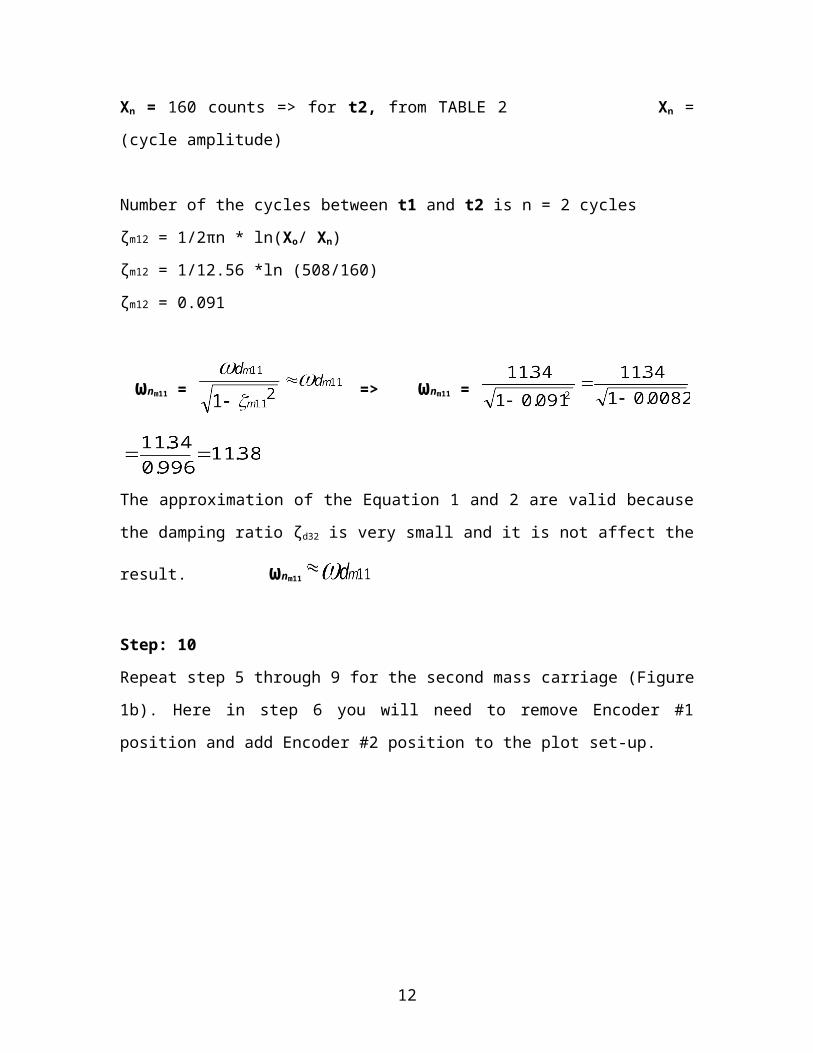
Xn = 160 counts => for t2, from TABLE 2 Xn = (cycle amplitude)
Number of the cycles between t1 and t2 is n = 2 cycles
ζm12 = 1/2πn * ln(Xo/ Xn)
ζm12 = 1/12.56 *ln (508/160)
ζm12 = 0.091
ωnm11 = => ωnm11 =
The approximation of the Equation 1 and 2 are valid because the damping ratio ζd32 is
very small and it is not affect the result. ωnm11
Step: 10
9
Repeat step 5 through 9 for the second mass carriage (Figure 1b). Here in step 6 you will
need to remove Encoder #1 position and add Encoder #2 position to the plot set-up.
Figure: 5 (load encoder # 2)
Hence obtain ωnm21, ωnm22, ζm22.
How does this damping ratio compare with that for the first mass?
This damping ratio is approximately 13 times lower than the damping ratio that we found
in step: 9
We choose,
t1 = 0.142 seconds 423 counts from TABLE 3
t2 = 1.213 seconds 388 counts from TABLE 3
so the number of the cycles between t1 and t2 is n = 2 cycles
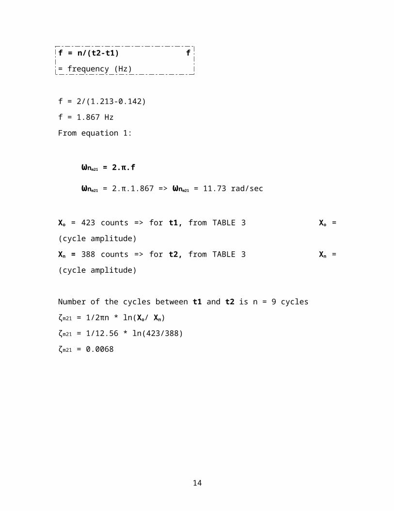
f = n/(t2-t1) f = frequency (Hz)
f = 2/(1.213-0.142)
10
f = 1.867 Hz
From equation 1:
ωnm21 = 2.π.f
ωnm21 = 2.π.1.867 => ωnm21 = 11.73 rad/sec
Xo = 423 counts => for t1, from TABLE 3 Xo = (cycle amplitude)
Xn = 388 counts => for t2, from TABLE 3 Xn = (cycle amplitude)
Number of the cycles between t1 and t2 is n = 9 cycles
ζm21 = 1/2πn * ln(Xo/ Xn)
ζm21 = 1/12.56 * ln(423/388)
ζm21 = 0.0068
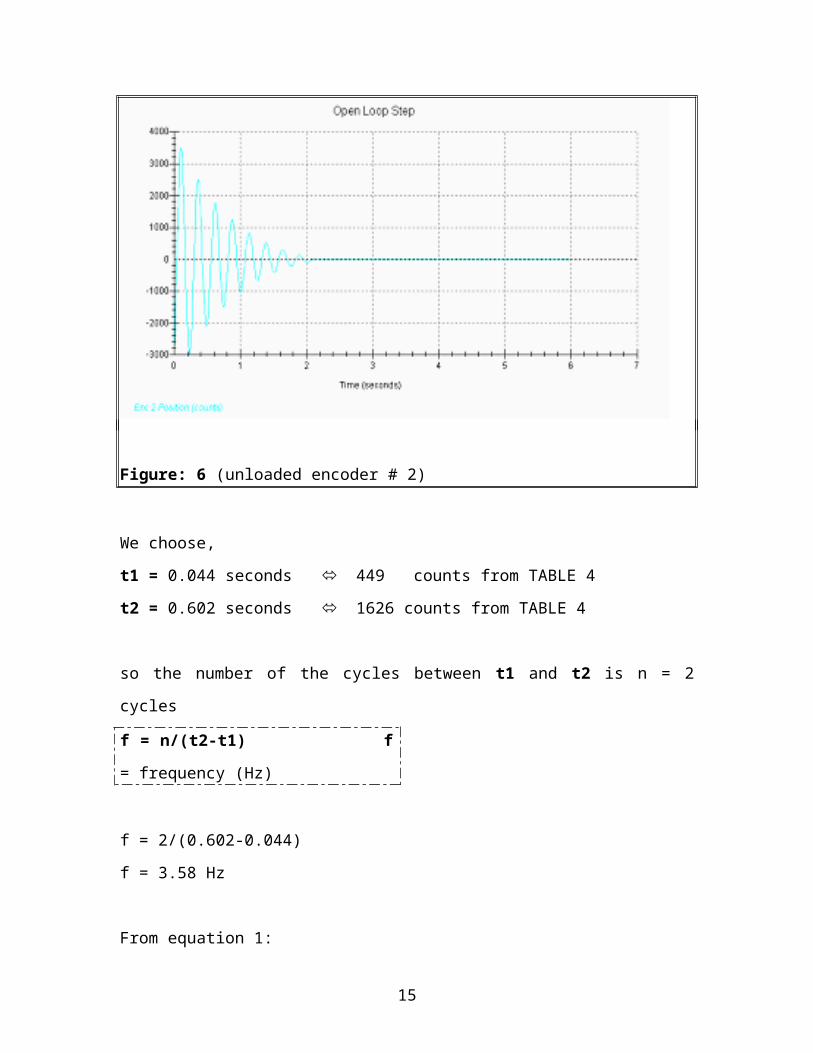
Figure: 6 (unloaded encoder # 2)
We choose,
t1 = 0.044 seconds 449 counts from TABLE 4
11
t2 = 0.602 seconds 1626 counts from TABLE 4
so the number of the cycles between t1 and t2 is n = 2 cycles
f = n/(t2-t1) f = frequency (Hz)
f = 2/(0.602-0.044)
f = 3.58 Hz
From equation 1:
ωnm22 = 2.π.f
ωnm22 = 2.π.3.58 => ωnm22 = 22.49 rad/sec
Xo = 1626 counts => for t1, from TABLE 4 Xo = (cycle amplitude)
Xn = 449 counts => for t2, from TABLE 4 Xn = (cycle amplitude)
Number of the cycles between t1 and t2 is n = 2 cycles
ζm22 = 1/2πn * ln(Xo/ Xn)
ζm22 = 1/12.56 * ln(1626/449)
ζm22 = 0.101
step: 11
Connect the mass carriage extension bracket and dashpot to the second mass as shown in
figure 1c. Open the damping (air flow) adjustment knob 2.0 turns from the fully closed
position. Repeat step 5, 6, and 9 with four 500g masses on the second carriage and using
only amplitudes 500 counts in your damping ratio calculation. Hence obtain ζd where
the “d” subscript denotes “dashpot”.
12
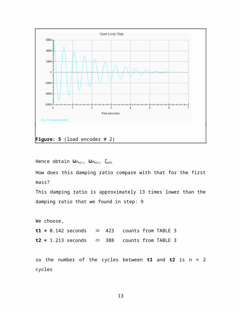
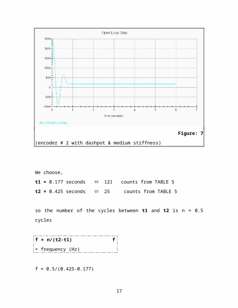
Figure: 7 (encoder # 2 with dashpot & medium stiffness)
We choose,
t1 = 0.177 seconds 121 counts from TABLE 5
t2 = 0.425 seconds 25 counts from TABLE 5
so the number of the cycles between t1 and t2 is n = 0.5 cycles
f = n/(t2-t1) f = frequency (Hz)
f = 0.5/(0.425-0.177)
f = 2.016 Hz
From equation 1:
ωd = 2.π.f
ωd = 2.π.2.016 => ωd = 12.66 rad/sec
13
Xo = 121 counts => for t1, from TABLE 5 Xo = (cycle amplitude)
Xn = 25 counts => for t2, from TABLE 5 Xn = (cycle amplitude)
Number of the cycles between t1 and t2 is n = 0.5 cycles
ζm21 = 1/2πn * ln(Xo/ Xn)
ζm21 = 1/3.14 * ln(121/25)
ζm21 = 0.50
Step: 12
Each brass weight has a mass of 500 10g. (you may weight the pieces if a more precise
value is desired). Calling the mass of the four weights combined mw, use the following
relationships to solve for the unloaded carriage mass mc2, and spring constant k.
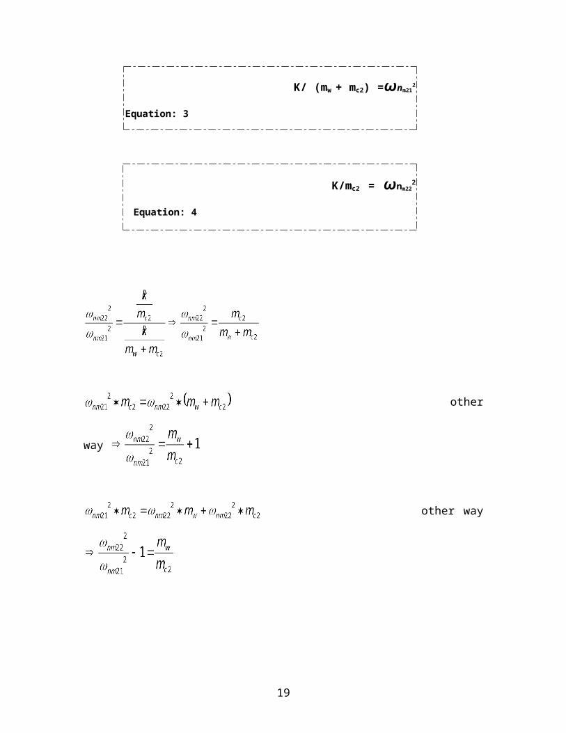
K/ (mw + mc2) =ωnm212 Equation: 3
K/mc2 = ωnm222 Equation: 4
other way
other way
14
other way
other way
other way
kg other way kg
we take the other way kg
rad/sec
N/m
find the damping coefficient cm2 by equating the first order terms in the equation form:
Equation: 5
from this equation,
N/Ms
repeat the above for the first mass carriage, spring and damping mc1, cm1 and k
respectively.
Calculate the damping coefficient of the dashpot, cd.
15
other way
other way
other way
other way
other way
kg other way kg
we take the other way kg
rad/sec
N/m
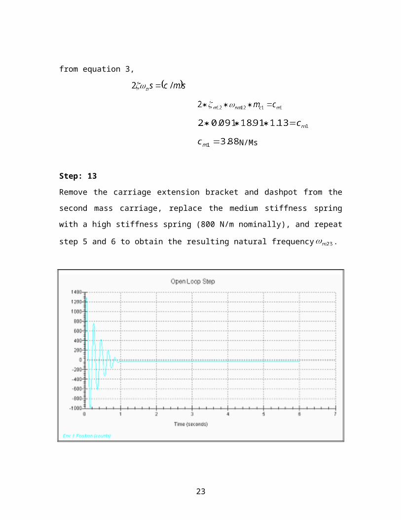
from equation 3,
16
N/Ms
Step: 13
Remove the carriage extension bracket and dashpot from the second mass carriage,
replace the medium stiffness spring with a high stiffness spring (800 N/m nominally), and
repeat step 5 and 6 to obtain the resulting natural frequency .
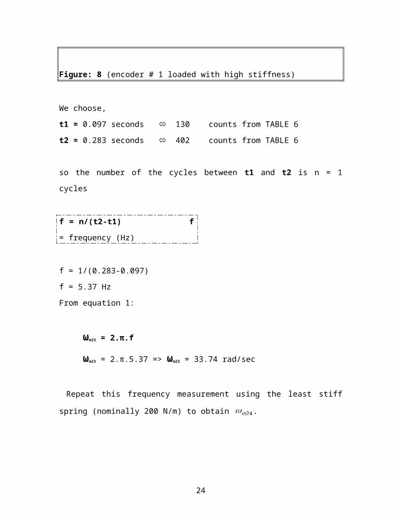
Figure: 8 (encoder # 1 loaded with high stiffness)
We choose,
t1 = 0.097 seconds 130 counts from TABLE 6
t2 = 0.283 seconds 402 counts from TABLE 6
so the number of the cycles between t1 and t2 is n = 1 cycles
f = n/(t2-t1) f = frequency (Hz)
f = 1/(0.283-0.097)
17
f = 5.37 Hz
From equation 1:
ωm23 = 2.π.f
ωm23 = 2.π.5.37 => ωm23 = 33.74 rad/sec
Repeat this frequency measurement using the least stiff spring (nominally 200 N/m) to
obtain .
Figure: 9 (encoder # 1 with low stiffness)
We choose,
t1 = 0.097 seconds 680 counts from TABLE 7
t2 = 0.390 seconds 299 counts from TABLE 7
so the number of the cycles between t1 and t2 is n = 1 cycles
f = n/(t2-t1) f = frequency (Hz)
18
f = 1/(0.390-0.097)
f = 3.41 Hz
From equation 1:
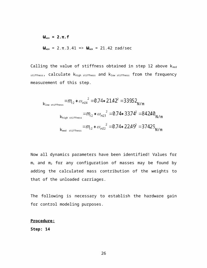
ωm24 = 2.π.f
ωm24 = 2.π.3.41 => ωm24 = 21.42 rad/sec
Calling the value of stiffness obtained in step 12 above kmed stiffness, calculate khigh stiffness and
klow stiffness from the frequency measurement of this step.
klow stiffness N/m
khigh stiffness N/m
kmed stiffness N/m
Now all dynamics parameters have been identified! Values for m1 and m2 for any
configuration of masses may be found by adding the calculated mass contribution of the
weights to that of the unloaded carriages.
The following is necessary to establish the hardware gain for control modeling purposes.
Procedure:
Step: 14
Remove the spring connecting the first and second masses and secure four 500g masses
on the first mass carriage. (you should libel this particular spring so that the identified
parameter k2 will be consistent when used in later experiments). Use the limit clamps to
secure the second mass clear from the first. Verify that the masses are secure and that the
carriage slides freely. Hook up the drive power to the mechanism. Position the first mass
approximately 3cm to the left (negative x1 position) of its center of travel.
19
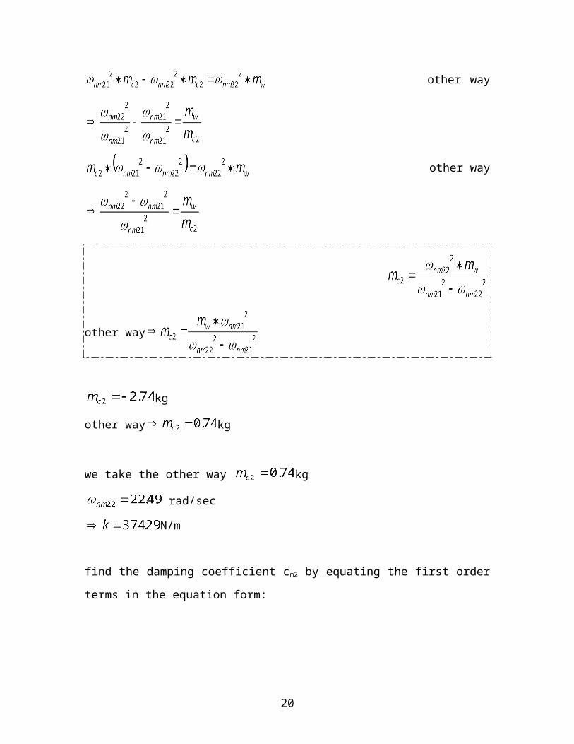
Figure: 10 (encoder # 1 loaded)
Step: 15
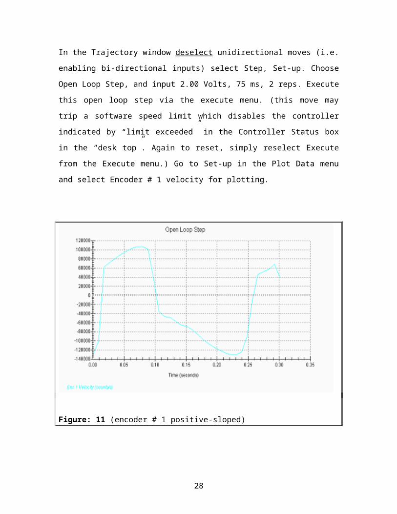
In the Trajectory window deselect unidirectional moves (i.e. enabling bi-directional
inputs) select Step, Set-up. Choose Open Loop Step, and input 2.00 Volts, 75 ms, 2 reps.
Execute this open loop step via the execute menu. (this move may trip a software speed
limit which disables the controller indicated by “limit exceeded” in the Controller Status
box in the “desk top”. Again to reset, simply reselect Execute from the Execute menu.)
Go to Set-up in the Plot Data menu and select Encoder # 1 velocity for plotting.
20
Figure: 11 (encoder # 1 positive-sloped)
Figure: 12 (encoder # 1 negative-sloped)
21
Step: 16
Plot this data and observe four velocity profile segments with nominal shapes of : linear
increase (constant acceleration), constant (zero acceleration), linear decrease
(deceleration), and constant. Obtain the acceleration, 1e, (counts/s2) by carefully
measuring the velocity difference and dividing by the time difference (75ms) through the
positive-sloped segment. Calculate the average magnitude of the positive and negative
accelerations for use in obtaining khw below.
The acceleration,
For positive linear segment = = 34666.66 counts/s2
For negative linear segment= = 546666.66 counts/s2
Therefore =
= 290666.66 counts/s2
Step: 17
Save any files or plots of interest. Exit the executive program and power down the
system.
Conclusion:
From the experiments that we have done we identified the plants parameters and
also there are some results between the damping frequency and the damping ratio. As we
can see in step 8 #3 and step 10 #2 (for the unloaded carriage the damping frequency are
almost the same) and in step 6 #3 and step 10 #2 the (damping frequency are almost the
same). The damping frequency for the first or second mass of unloaded cases is
approximately the double in the cases of loaded mass. The mechanical connection of
former with the motor causes frictional forces to act on it and therefore, the damping ratio
of the first mass is more than the second mass. In the cases where a dashpot is connected
22
the damping frequency is decreased because of the forces that acting on the mass
carriage.
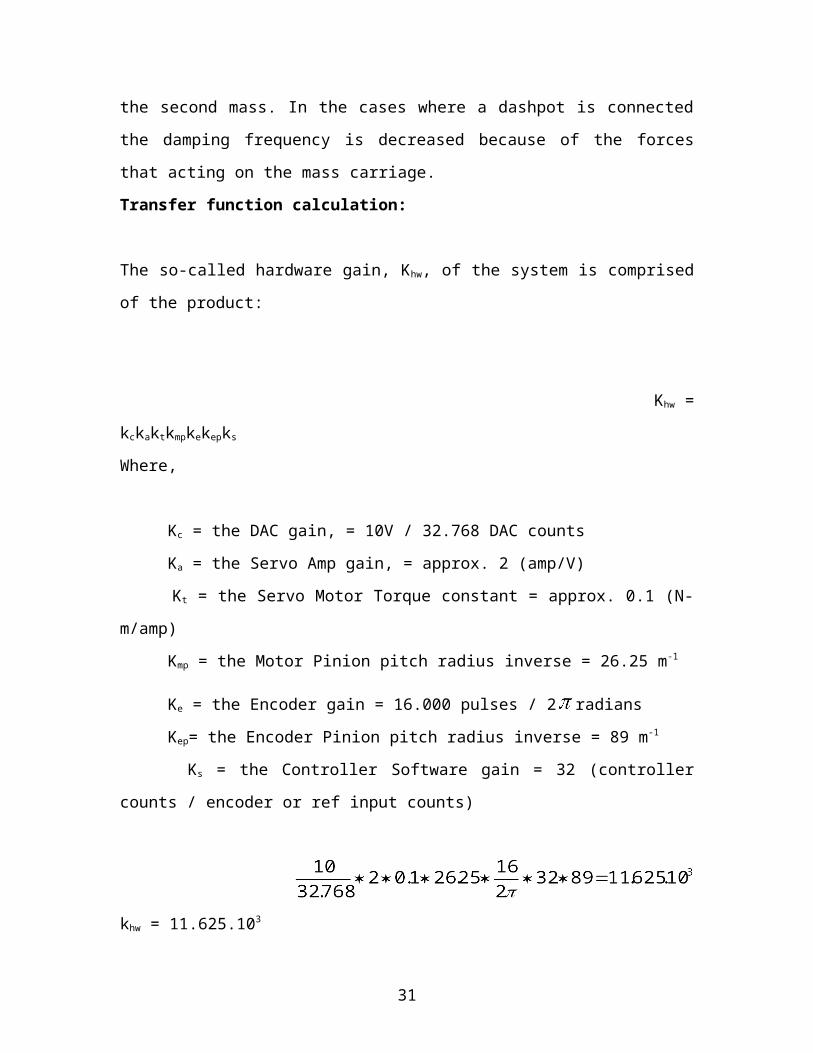
Transfer function calculation:
The so-called hardware gain, Khw, of the system is comprised of the product:
Khw = kckaktkmpkekepks
Where,
Kc = the DAC gain, = 10V / 32.768 DAC counts
Ka = the Servo Amp gain, = approx. 2 (amp/V)
Kt = the Servo Motor Torque constant = approx. 0.1 (N-m/amp)
Kmp = the Motor Pinion pitch radius inverse = 26.25 m-1
Ke = the Encoder gain = 16.000 pulses / 2 radians
Kep= the Encoder Pinion pitch radius inverse = 89 m-1
Ks = the Controller Software gain = 32 (controller counts / encoder or ref input counts)
khw = 11.625.103
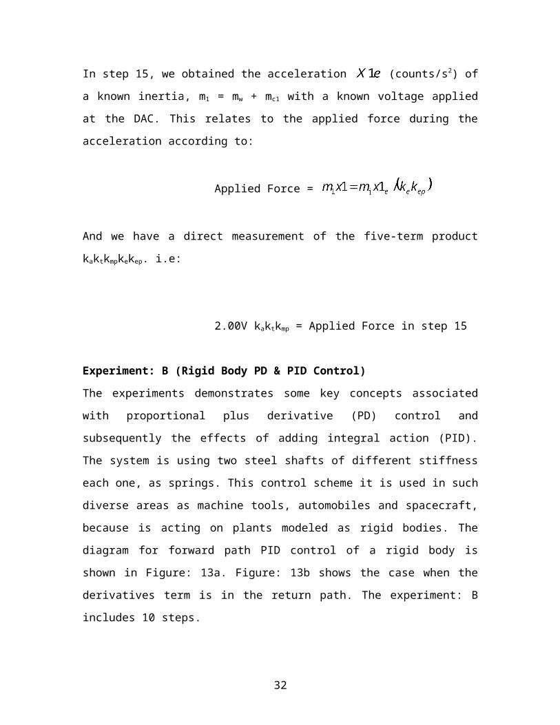
In step 15, we obtained the acceleration (counts/s2) of a known inertia, m1 = mw +
mc1 with a known voltage applied at the DAC. This relates to the applied force during the
acceleration according to:
Applied Force =
And we have a direct measurement of the five-term product kaktkmpkekep. i.e:
2.00V kaktkmp = Applied Force in step 15
23
Experiment: B (Rigid Body PD & PID Control)
The experiments demonstrates some key concepts associated with proportional plus
derivative (PD) control and subsequently the effects of adding integral action (PID). The
system is using two steel shafts of different stiffness each one, as springs. This control
scheme it is used in such diverse areas as machine tools, automobiles and spacecraft,
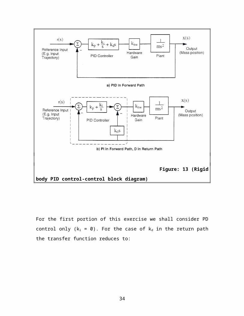
because is acting on plants modeled as rigid bodies. The diagram for forward path PID
control of a rigid body is shown in Figure: 13a. Figure: 13b shows the case when the
derivatives term is in the return path. The experiment: B includes 10 steps.
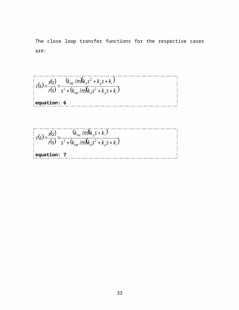
The close loop transfer functions for the respective cases are:
equation: 6
equation: 7
24
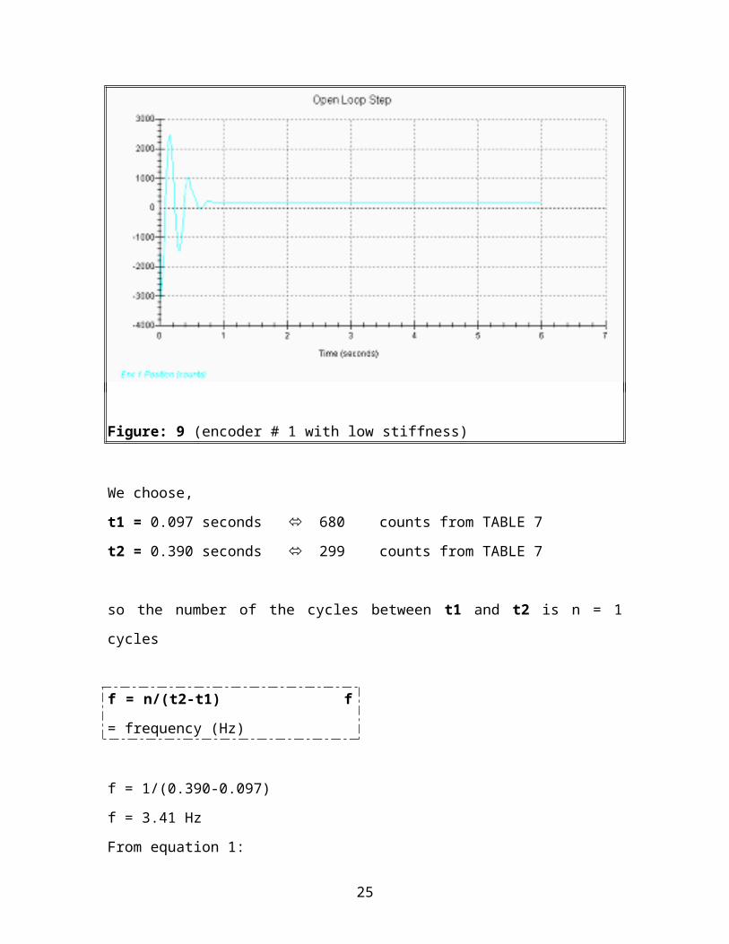
Figure: 13 (Rigid body PID control-control block diagram)
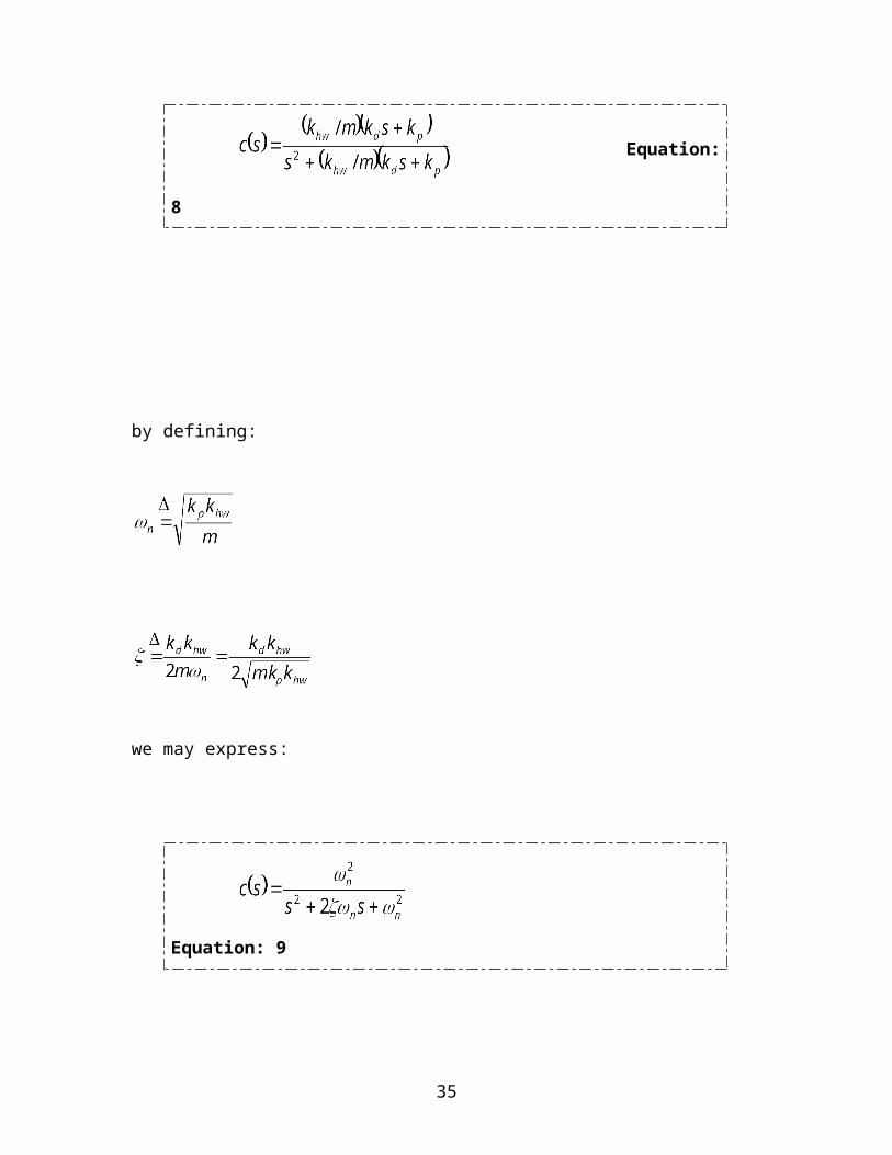
For the first portion of this exercise we shall consider PD control only (k i = 0). For the
case of kd in the return path the transfer function reduces to:
Equation: 8
25
by defining:
we may express:
Equation: 9
the effect of kp and kd on the roots of the denominator (damped second order oscillator) of
c(s) is studied in the work that follows.
Procedure: (Proportional & Derivative Control Actions)
Step: 1
Using the result of experiment A construct a model of the plant with four 500g mass
pieces on the first mass carriage with no springs or damper attached. You may neglect
friction.
Step: 2
Set-up the plant in the configuration described in Step 1. There should be no springs or
damper connected to the first carriage and the other carriages should be secured away
from the range of motion of the first carriage.
26

Step: 3
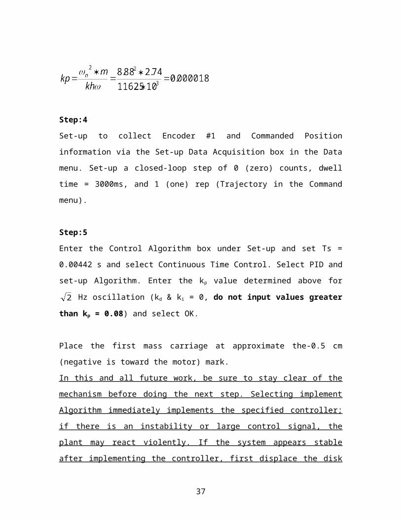
From Eq determine the value of kp (kd = 0) so that the system behaves like a Hz
spring-mass oscillator.
Step:4
Set-up to collect Encoder #1 and Commanded Position information via the Set-up Data
Acquisition box in the Data menu. Set-up a closed-loop step of 0 (zero) counts, dwell
time = 3000ms, and 1 (one) rep (Trajectory in the Command menu).
Step:5
Enter the Control Algorithm box under Set-up and set Ts = 0.00442 s and select
Continuous Time Control. Select PID and set-up Algorithm. Enter the kp value
determined above for Hz oscillation (kd & ki = 0, do not input values greater than
kp = 0.08) and select OK.
Place the first mass carriage at approximate the-0.5 cm (negative is toward the motor)
mark.
In this and all future work, be sure to stay clear of the mechanism before doing the next
step. Selecting implement Algorithm immediately implements the specified controller; if
there is an instability or large control signal, the plant may react violently. If the system
appears stable after implementing the controller, first displace the disk with a light, non
sharp object (e.g. a plastic ruler) to verify stability prior to touching plant
Select Implement Algorithm, then OK.
27
Step:6
Select Execute under Command. Prepare to manually displace the mass carriage roughly
2 cm. Select Run, displace the mass approximately 3 cm and release it. Do not hold the
mass position for longer than about 1 second as this may cause the motor drive thermal
protection to open the control loop.
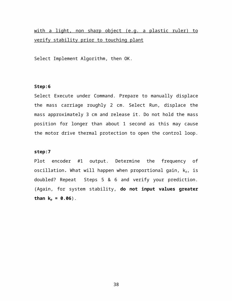
step:7
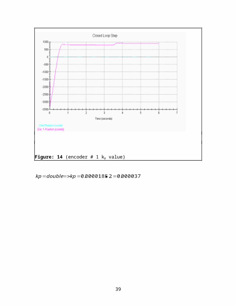
Plot encoder #1 output. Determine the frequency of oscillation. What will happen when
proportional gain, kp, is doubled? Repeat Steps 5 & 6 and verify your prediction. (Again,
for system stability, do not input values greater than kp = 0.06).
Figure: 14 (encoder # 1 kp value)
28
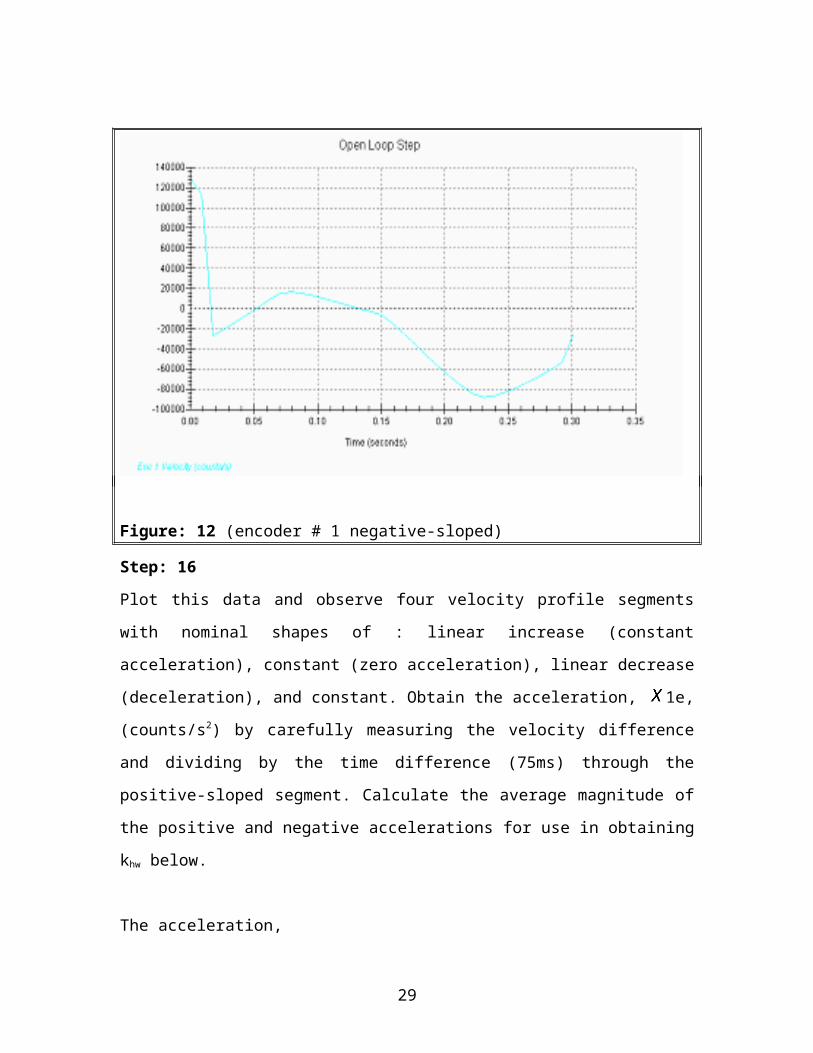
Figure: 15 (encoder # 1 kp double value)
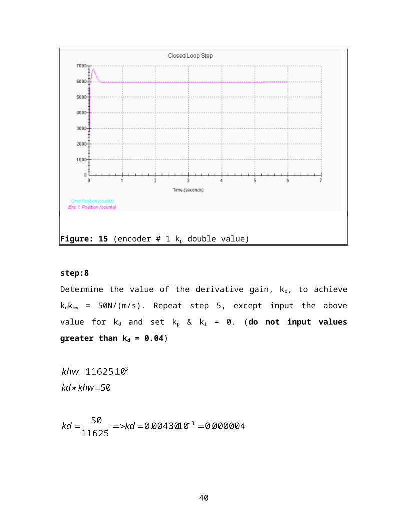
step:8
Determine the value of the derivative gain, kd, to achieve kdkhw = 50N/(m/s). Repeat step
5, except input the above value for kd and set kp & ki = 0. (do not input values greater
than kd = 0.04)
29
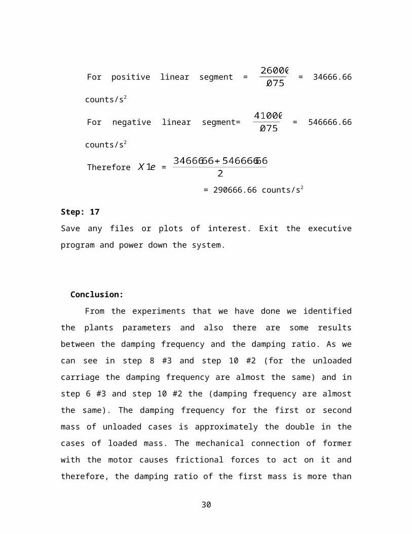
Figure: 16 (encoder # 1 kd value)
step:9
After checking the system for stability by displacing it with a ruler, manually move the
mass back and forth to feel the effect of viscous damping provided by kd. Do not
excessively coerce the mass as this will again cause the motor drive thermal protection to
open the control loop.
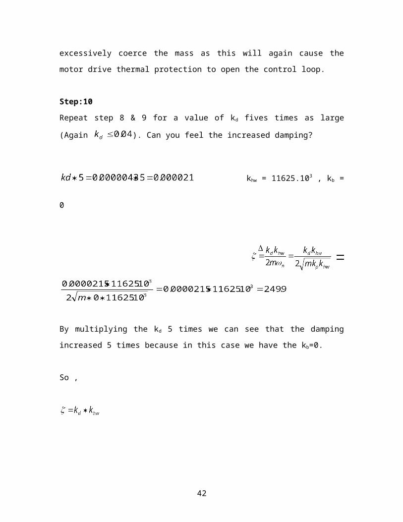
Step:10
Repeat step 8 & 9 for a value of kd fives times as large (Again ). Can you feel
the increased damping?
khw = 11625.103 , kb = 0
30
By multiplying the kd 5 times we can see that the damping increased 5 times because in
this case we have the kb=0.
So ,
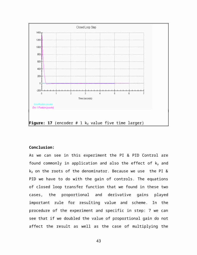
Figure: 17 (encoder # 1 kd value five time larger)
Conclusion:
As we can see in this experiment the PI & PID Control are found commonly in
application and also the effect of kp and kd on the roots of the denominator. Because we
use the PI & PID we have to do with the gain of controls. The equations of closed loop
transfer function that we found in these two cases, the proportional and derivative gains
played important rule for resulting value and scheme. In the procedure of the experiment
31
and specific in step: 7 we can see that if we doubled the value of proportional gain do not
affect the result as well as the case of multiplying the derivative gain five times as large
in step: 10. Finally in this experiment we can see the behavior of the second order-
system.
32
EXERIMENT: A
TABLE: 1 (DATA FROM STEP: 6)
Sample time encoder # 1 pos
38 0.336 304
39 0.345 637
40 0.354 957
41 0.363 1263
42 0.372 1553
43 0.381 1821
44 0.390 2069
45 0.398 2293
46 0.407 2489
47 0.416 2656
. . .
. . .
. . .
. . .
. . .
163 1.443 2
164 1.452 38
165 1.461 72
166 1.470 103
167 1.479 131
168 1.488 155
169 1.496 176
170 1.505 193
171 1.514 206
172 1.523 215
33
EXERIMENT: A
TABLE: 2 (DATA FROM STEP: 8)
Sample time encoder # 1 pos
6 0.053 508
7 0.062 972
8 0.071 1388
9 0.080 1744
10 0.089 2027
11 0.097 2230
12 0.106 2344
13 0.115 2370
14 0.124 2308
15 0.133 2168
. . .
. . .
. . .
. . .
. . .
76 0.673 125
77 0.682 146
78 0.691 159
79 0.699 165
80 0.708 166
81 0.717 160
82 0.726 148
83 0.735 133
84 0.744 116
85 0.753 98
34
EXERIMENT: A
TABLE: 3 (DATA FROM STEP: 10)
Sample time encoder # 2 pos
7 0.062 4882
8 0.071 4520
9 0.080 4112
10 0.089 3663
11 0.097 3179
12 0.106 2664
13 0.115 2125
14 0.124 1567
15 0.133 998
16 0.142 423
. . .
. . .
. . .
. . .
. . .
129 1.142 3008
130 1.151 2752
131 1.160 2469
132 1.169 2162
133 1.178 1834
134 1.186 1489
135 1.195 1130
136 1.204 762
137 1.213 388
138 1.222 13
35
EXERIMENT: A
TABLE: 4 (DATA FROM STEP: 10unload)
Sample time encoder # 2 pos
5 0.044 449
6 0.053 1228
7 0.062 1933
8 0.071 2534
9 0.080 3006
10 0.089 3328
11 0.097 3490
12 0.106 3490
13 0.115 3330
14 0.124 3023
. . .
. . .
. . .
. . .
. . .
63 0.558 57
64 0.567 463
65 0.576 839
66 0.584 1167
67 0.593 1433
68 0.602 1626
69 0.611 1738
70 0.620 1767
71 0.629 1715
72 0.638 1584
36
EXERIMENT: A
TABLE: 5 (DATA FROM STEP: 11)
Sample time encoder # 2 pos
11 0.097 1688
12 0.106 1525
13 0.115 1355
14 0.124 1179
15 0.133 999
16 0.142 818
17 0.151 637
18 0.159 459
19 0.168 287
20 0.177 121
. . .
. . .
. . .
. . .
. . .
48 0.425 25
49 0.434 101
50 0.443 174
51 0.452 244
52 0.460 310
53 0.469 372
54 0.478 429
55 0.487 481
56 0.496 527
57 0.505 567
37
EXERIMENT: A
TABLE: 6 (DATA FROM STEP: 13hi)
Sample time encoder # 1 pos
2 0.018 746
3 0.027 1024
4 0.035 1202
5 0.044 1290
6 0.053 1278
7 0.062 1160
8 0.071 956
9 0.080 712
10 0.089 431
11 0.097 130
. . .
. . .
. . .
. . .
. . .
25 0.221 404
26 0.230 578
27 0.239 701
28 0.248 760
29 0.257 745
30 0.266 672
31 0.274 554
32 0.283 402
33 0.292 227
34 0.301 41
38
EXERIMENT: A
TABLE: 7 (DATA FROM STEP: 13le)
Sample time encoder # 1 pos
10 0.089 166
11 0.097 680
12 0.106 1131
13 0.115 1536
14 0.124 1879
15 0.133 2149
16 0.142 2339
17 0.151 2441
18 0.159 2456
19 0.168 2385
. . .
. . .
. . .
. . .
. . .
43 0.381 39
44 0.390 299
45 0.398 544
46 0.407 722
47 0.416 844
48 0.425 935
49 0.434 991
50 0.443 1010
51 0.452 996
52 0.460 950
39
EXERIMENT: A
TABLE: 8 (DATA FROM STEP: 14)
Sample time encoder # 1 pos
1 0.009 5832
2 0.018 5615
3 0.027 5347
4 0.035 5032
5 0.044 4671
6 0.053 4269
7 0.062 3831
8 0.071 3360
9 0.080 2862
10 0.089 2343
. . .
. . .
. . .
. . .
. . .
46 0.407 265
47 0.416 700
48 0.425 1122
49 0.434 1529
50 0.443 1918
51 0.452 2283
52 0.460 2622
53 0.469 2930
54 0.478 3206
55 0.487 3445
40
EXERIMENT: A
TABLE: 9 (DATA FROM STEP: 15po)
Sample time encoder # 1 pos
5 0.044 229
6 0.053 1059
7 0.062 1951
8 0.071 2889
9 0.080 3858
10 0.089 4788
11 0.097 5662
12 0.106 5463
13 0.115 5035
14 0.124 4631
. . .
. . .
. . .
. . .
. . .
23 0.204 -2074
24 0.213 -3174
25 0.221 -4320
26 0.230 -5509
27 0.239 -6655
28 0.248 -7729
29 0.257 -8254
30 0.266 -7899
31 0.274 -7446
32 0.283 -6981
41
EXERIMENT: A
TABLE: 10 (DATA FROM STEP: 15ne)
Sample time encoder # 1 pos
0 0.000 2620
1 0.009 2297
2 0.018 2026
3 0.027 1813
4 0.035 1663
5 0.044 1578
6 0.053 1558
7 0.062 1600
8 0.071 1704
9 0.080 1861
. . .
. . .
. . .
. . .
. . .
23 0.204 360
24 0.213 -282
25 0.221 -1000
26 0.230 -1783
27 0.239 -2566
28 0.248 -3321
29 0.257 -4043
30 0.266 -4719
31 0.274 -5347
32 0.283 -5920
42
EXERIMENT: B
TABLE: 1 (DATA FROM STEP: 7)
Sample time encoder # 1 pos
0 0.000 -3377
1 0.009 -3293
2 0.018 -3212
3 0.027 -3134
4 0.035 -3061
5 0.044 -2992
6 0.053 -2927
7 0.062 -2866
8 0.071 -2810
9 0.080 -2756
. . .
. . .
. . .
. . .
. . .
51 0.452 28
52 0.460 80
53 0.469 129
54 0.478 176
55 0.487 221
56 0.496 265
57 0.505 308
58 0.514 351
59 0.522 392
60 0.531 433
43

EXERIMENT: B
TABLE: 2 (DATA FROM STEP: 7)
Sample time encoder # 1 pos
0 0.000 5463
1 0.009 5584
2 0.018 5702
3 0.027 5817
4 0.035 5931
5 0.044 6041
6 0.053 6150
7 0.062 6256
8 0.071 6359
9 0.080 6460
. . .
. . .
. . .
. . .
. . .
41 0.363 5962
42 0.372 5954
43 0.381 5947
44 0.390 5942
45 0.398 5937
46 0.407 5934
47 0.416 5931
48 0.425 5930
49 0.434 5929
50 0.443 5929
44
EXERIMENT: B
TABLE: 3 (DATA FROM STEP: 8)
Sample time encoder # 1 pos
0 0.000 -1062
1 0.009 -992
2 0.018 -924
3 0.027 -858
4 0.035 -794
5 0.044 -732
6 0.053 -671
7 0.062 -611
8 0.071 -554
9 0.080 -498
. . .
. . .
. . .
. . .
. . .
46 0.407 299
47 0.416 296
48 0.425 292
49 0.434 289
50 0.443 286
51 0.452 284
52 0.460 282
53 0.469 281
54 0.478 280
55 0.487 280
45
EXERIMENT: B
TABLE: 4 (DATA FROM STEP: 10)
Sample time encoder # 1 pos
0 0.000 1419
1 0.009 1336
2 0.018 1256
3 0.027 1179
4 0.035 1105
5 0.044 1035
6 0.053 968
7 0.062 903
8 0.071 840
9 0.080 779
. . .
. . .
. . .
. . .
. . .
45 0.398 -13
46 0.407 -13
47 0.416 -12
48 0.425 -11
49 0.434 -11
50 0.443 -10
51 0.452 -9
52 0.460 -9
53 0.469 -8
54 0.478 -8
46