Advertising Budget And Sales Paths Under The Dynamics Of

San Jose State University San Jose State University

SJSU ScholarWorks SJSU ScholarWorks

Faculty Publications Marketing and Decision Sciences

1-1-2012

Advertising Budget And Sales Paths Under The Dynamics Of The Advertising Budget And Sales Paths Under The Dynamics Of The

Student Work Control Problem And Regularity Requirements Student Work Control Problem And Regularity Requirements

Aharon Hibshoosh San Jose State University, [email protected]

Follow this and additional works at: https://scholarworks.sjsu.edu/mktds_pub

Part of the Marketing Commons

Recommended Citation Recommended Citation Aharon Hibshoosh. "Advertising Budget And Sales Paths Under The Dynamics Of The Student Work Control Problem And Regularity Requirements" Journal of Business & Economics Research (2012): 463-483.

This Article is brought to you for free and open access by the Marketing and Decision Sciences at SJSU ScholarWorks. It has been accepted for inclusion in Faculty Publications by an authorized administrator of SJSU ScholarWorks. For more information, please contact [email protected].

https://scholarworks.sjsu.edu/

https://scholarworks.sjsu.edu/mktds_pub

https://scholarworks.sjsu.edu/mktds

https://scholarworks.sjsu.edu/mktds_pub?utm_source=scholarworks.sjsu.edu%2Fmktds_pub%2F7&utm_medium=PDF&utm_campaign=PDFCoverPages

http://network.bepress.com/hgg/discipline/638?utm_source=scholarworks.sjsu.edu%2Fmktds_pub%2F7&utm_medium=PDF&utm_campaign=PDFCoverPages

mailto:[email protected]

Journal of Business & Economics Research – August 2012 Volume 10, Number 8

© 2012 The Clute Institute http://www.cluteinstitute.com/ 463

Advertising Budget And Sales Paths

Under The Dynamics Of The Student

Work Control Problem

And Regularity Requirements Aharon Hibshoosh, San Jose State University, USA

ABSTRACT

Consider a firm promoting a product in a fast expanding industry by using advertising as its

single promotional tool. The firm’s objective is to minimize the overall cost of advertising

necessary for reaching certain target sales of the product by the end of a given planning period.

We adopt the Student Work Control problem (SWC) framework for modeling this marketing

context, in general, and the advertising-sales response function, in particular. We compare the

SWC’s optimal control budgeting principle with the solutions of equally effective, alternative

advertising budgeting principles, which require strong regularity conditions on the path of either

the advertising outlays or sales. In contrast to the other principles, SWC’s optimal sales path is

highly convex to the point that the firm may deliberately accept decreasing sales at the earliest

periods. However, its optimal solution requires the firm to advertise in every period and to

continue to accelerate its advertising outlays. The resulting Advertising Sales Response function,

too, may therefore have a convex section with declining sales, a finding contributing to an

optimization-driven explanation of threshold in advertising effect on sales.

Keywords: Student Work Control Problem; Advertising Budgeting; Advertising-Sales Response; Regularity

Conditions

INTRODUCTION

onsider a firm marketing a product in a fast expanding industry in the introduction or the early growth

stage of a product life cycle. The firm’s objective is reaching a certain level of sales, within a pre-

specified planning window, in an efficient and regular manner. In general, a firm facing its sales growth

dynamics would apply its whole optimal marketing mix. However, in this paper, as is often common in marketing,

in modeling sales response to advertising, we treat advertising as the firm’s sole decision variable, assuming the role

of the rest of the decision variables implicitly. We follow Buratto and Viscolani (1994) in adopting and extending

the framework of the Student Work Control problem (SWC) (Raggett, Hempson and Jukes, 1981) for discreetly

modeling this marketing context. In particular, we rely on a straightforward extension of the SWC by Klamkin

(1985) in flexibly modeling advertising efficiency. For recent continuous extensions of the SWC, see Vornicescu

(2009).

Buratto and Viscolani assumed the marketing context of launching a new product where advertising is

building goodwill. In contrast, we deal with a product in the introduction or early growth stage, where advertising

builds sales, and thus consider different planning implications. Hence, unlike the focus of Buratto and Viscolani on

relaxing the assumption of a fixed planning window, our emphasis is on modification and extension of the SWC for

the case where the control is restricted not only by the problem’s dynamics, but also by regularity conditions on

either sales or advertising paths, brought about by abiding by alternative advertising budgeting principles.

C


464 http://www.cluteinstitute.com/ © 2012 The Clute Institute

In common with earlier classical approaches to modeling the sales response function to advertising of

Nerlove and Arrow (1962), Vidal and Wolfe (1957), the dynamics in the SWC are flexibly representing sales

momentum and a decaying of the effect of past sales. However, unlike Nerlove and Arrow, we do not model a case

where advertising builds an intervening variable (goodwill) without diminishing returns. In our modeling, the role

of intervening variables is subsumed and we assume diminishing return of sales as advertising increases. Neither

do we model the case where effectiveness of advertising depends on a market potential as it is modeled by Vidal and

Wolfe. When the product is in its growth stage in the product life cycle or is marketed in a fast expanding industry,

the evolving product potential is affected by strategic marketing decisions and its assessment is not stable. Hence, in

this expository paper, we also chose not to model strategic behavior and, in particular, the pursuit of market share,

though we share with Yoo and Mandhachitara (2003) and Miller and Pazgal (2007) the perspective that advertising

budgeting principles have material effect on the firm’s competitive performance. Instead, we model a credible, but

modeling-wise overlooked, objective for a firm in its introductory or early growth stage—a timely attainment of a

prescribed sales level. This attainment may be necessary, for example, in order to arrive at required capacity

utilization to reach some desired level of market presence or to secure some critical financial support.

In general, for coherent planning, firms are interested in resource employment and sales paths that possess

some degree of regularity. The efficiency of reaching any target sales using any advertising control depends on the

budgeting principle of the control. The classical list of advertising budgeting principles has been a short one. It

typically includes: 1) the Objective and Task principle, a universally tautologically effective and efficient optimal

method that is objective-specific, 2) the straight forward and regular, but not necessarily, optimal principles of the

Percentage of Sales methods and the Competitive Parity method, and 3) the Affordable Budget method. The

comparative parity method tends to be regular because industry practices tend to evolve gradually, but it is not

associated with a particular formal regularity condition on the advertising budget that is internal to the firm. The

affordable method satisfies feasibility, but not regularity or optimality of the path. With the exception of the

percentage of sales methods, the other “textbook” advertising budgeting principles are not inherently based on any

internal firm’s regularity.

In this paper, we also consider new additional reference principles that embody benchmark regularity in

advertising and sales. These regularity conditions require either constant or proportional increments from one

period to the next, in either the advertising budget or sales. They are equivalent to requiring a linear temporal path,

or alternatively, a geometrically progressing one. Those assumptions are made on either the advertising budget path

or on the sales path, but not on both, to avoid contradiction.

Our interest in the effects of regularity conditions is motivated, in part, by recognition that regularity

conditions, coupled with the dynamics of advertising-sales relationship, often uniquely determine the optimal

advertising control and its related sales path. An insightful result of our study is that requiring a constant rate of

growth on the advertising path uniquely (and easily) determines the optimal control of the SWC problem. It is thus

identical to the Objective and Task budgeting principle.

The main objective of the paper is to compare the consequences that alternative regularity conditions on the

sales path have on the advertising path and vice versa. Applying this inquiry to the characteristic marketing context

of this paper, as described by the SWC, would contribute to a sharper advertising budget planning. We are not aware

of any study that assumes this line of inquiry, though our study supplements a thorough research stream

investigating the role and effect of promotion budgeting by Wagner, Fischer, Albers and Frie in Wagner (2011).

In contrast to the instructive focus of their traditional classification, we view the key differences among the

budgeting principles as not primarily rooted in the effectiveness of the principle –“the Goal versus Non-goal

Attainment” - but rather in the efficiency of attaining the goal subject to its constraints, particularly ‘regularity

constraints’.

Actual media budgeting and planning practices motivate and support our perspective. In his UK-based

study of multinational firms, Mitchell (1993) has found great discrepancy between the classical list of advertising

budgeting principles and the actually applied principles. He reported that, in practice, firms are employing a large

number of varied principles which are closely aligned with the marketing purpose of the adverting.



Yet, in Low and Mohr’s (1999) study of the process of setting advertising budgets, the authors observed

that the budgeting principles are formed through complex negotiations, through traditional reference to historical

precedence of previously employed principles, and to the way of doing business. They concluded that these

practices often result in substantial inefficiencies.

Quite often a not-too-overly-complex-or-irregular budgeting principle would be agreed upon. In particular,

the finance and accounting parties in the negotiation, for whom regularity in budgeting is a common requirement,

are likely to push for budgets with easily decomposable components. Adjustments in accounting and finance are

typically comprised of components and procedures which are linear or reflecting constant rates of growth or

depreciation. We thus modeled our additional reference budgeting principles accordingly. Finding out whether or

how regularity requirements on an advertising path affect the regularity of the sales path or vice versa is clearly of

considerable interest.

Following these observations, we took two steps to provide insightful comparison of budgeting principles.

First, to facilitate a clearer efficiency comparison, we assume that the sales target is reached by all methods. This

requirement was sufficient for the unique determination of an optimal advertising path and a corresponding unique

optimal sales path for every budgeting principle compared. In the second step, for every budgeting principle, we

derived, where practical, analytical expressions of these optimal solutions. Obtaining explicit path solutions enabled

meaningful analytical inquiry of solution properties and eased comparisons and simulations. For instance, we prove

that the optimal advertising and sales paths of the Objective and Task principle are strongly convex. However,

counter intuitively, perhaps, the sales path need not be monotonic. While the firm is continually increasing its

advertising, it may let sales fall for a while before it begins to rise exponentially. In contrast, the optimal advertising

and sales paths, based on the Percentage of Sales principles, result in concave sales path pattern that is, as expected,

considerably more expensive than that obtained by the Objective and Task method.

The results of this study also supplement the arguments which explain why advertising elasticity is not

constant. Previous studies put the focus on the temporal variation of consumer awareness and involvement. Our

study complements by implying the joint role of the communicative effect of decaying habitual purchases, consumer

experimentation of new products, and the optimality principle of not allocating large advertising outlays when the

target is too distant and the profit margin is accelerating rapidly.

PROMOTION-ORIENTED ADAPTATION OF THE SWC

We model a firm marketing its product in the introduction stage or in the early part of the growth stage of

the product’s life cycle. As sales expand, the product may move from losses to profits and subsequently its profit

and profit margin are highly accelerating. Our base model is essentially a reinterpretation and further analysis of

one of several SWC’s extensions, proposed in the seminal paper of Raggett, Hempson and Jukes (1981).

We model Sales dynamics discretely. The index k, k= 1,…M, denotes the period (day, month, quarter),

where M is the length of the planning period. We denote the sales level at period k as kS and 0S is the initial sales

level. We assume one control variable, a planned advertisement spending in constant dollars, for period k, denoted

ask

U . The model dynamics is given as:

11 kkk bUaSS (1)

i.e., the sales level in any current period is a function of sales level in the preceding period and the advertising

budget for the current period. On the parameters values, we assume:

0 < a< 1 (2)

b >0 (3)



0< <1 (4)

These assumptions reflect common assumptions in the consumer behavior and promotion literature in

Marketing. Namely, there is imperfect sales inertia whose effect is gradually decaying over time. In addition, next

period sales are affected positively by the size of the next period advertising expenditures. This effect on sales

exhibits diminishing returns. The model implies that current period advertising has also an indirect positive carry-

over effect on future sales. However, this effect gradually decays over time.

The assumption of sales decay does not negate fast growth and sales momentum. However, it limits and

thus clarifies SWC’s range of application. It implies that the overall purchase of the current customer population

(rather than that of the individual) must decline from one period to the next when the product price is constant. This

is likely to be the case when the product is not frequently consumed. This is common in a wide array of marketing

contexts, for example, when the product is a durable good, a shopping good, a special experience, or a special

service. Consider, for example, the purchase of new sport exercise equipment, new consumer electronic devices,

new airline routes, new types of vacations, new types of financial services, etc. In contrast, if the product is

frequently purchased, the learning customer unit may increase rather than decrease its average consumption as its

use and satisfaction increase. In this case, our SWC’s version does not provide a valid representation of the

marketing context.

When the SWC applies, much of the sales momentum may come from the purchase by new customers

through product diffusion and adoption that may be directly and indirectly positively affected by the purchases by

old consumers via various communication modes. Hence, the expression, kaS , would not usually represent the

purchase by the old customers in the current period but rather a current purchase that is related to the size of the

quantity purchased by the old customers in the preceding period. It includes current purchases of new customers

and repeated purchases of old customers. Notice that over time, though, the future purchase of the population’s old

customers could be higher than their initial purchase through a multiplier effect. Our SWC model applies as long as

the current sales induced by past purchases would be smaller than past sales. There are common circumstances

where the effect of past purchases alone is so large that sales may accelerate without any advertising. In these cases,

our model is not valid.

The lack of universal application of the SWC model is a strength rather than a weakness. It qualifies the

effect of advertising and provides a balanced view of promotion. Much of the growth in the next period may be a

result of the effect of past purchases rather than due to current advertising. Furthermore, we do not assume that

advertising is responsible for the initial sales level. Many small enterprises cannot originally afford advertising

expense and their sales are initially built up by other promotional means. However, they often may turn to

advertising once some minimal sales level is reached in order to accelerate sales. Advertising is thus needed to

support sales expansion, though it may or may not be the main force behind this expansion. As a result of the

functioning of the advertising, it may be the increasing extent of customers’ experiences with the product that keeps

propelling the product’s sales higher.

The specific functional form of the dynamics has some attractive parsimonious conceptual and

measurement properties. The rate of decay, a, in the effect of current sales on next period’s sales is fixed. Thus,

Sales are conceptually conceived as the “depreciating capital” of the firm reflecting modern marketing focus on

customers’ equity and retention. The amount of the efficiency units of the advertising budget is U . The

parameter, b, provides a direct measure of the effect of an efficiency unit of the advertising budget (i.e., a unit of U ) on sales. The parameter , as a fraction, represents the diminishing return of advertising effect on current

sales. Specifically, we assume that the net current sales increment, not explained by past sales purchases, is a

constant elasticity function of current advertising budget outlay. This implies that advertising elasticity varies over

time with regularity as the product life cycle evolves and advertising expenditures change—a widely empirically

supported phenomena (see Sethuraman, Tellis, and Briesch, 2011).



We further assume that the marketer’s firm has the goal of achieving a target sales level M

M SS by the

end of the of the Mth period, with the obvious restriction of reaching higher sales, 0SS M . The planner’s

objective is to minimize the total advertising cost (in constant dollars) for the whole planning period, M

iUU1

.

Formally the problem can be summarized as

Min M

iUU1

subject to

11

kkkbUaSS

with 0<a<1, b >0 and 0< <1.

(5)

The key feature of our model adaptation is the assumption of sales as a state variable whose level is

ultimately affected by advertising. Planners commonly perceive the ultimate goal of advertising as sales increase.

Advertising usually affects an only partially observable complex communication process, with many interrelated

intervening variables, which eventually affects sales, although, on occasion, the mere act of advertising may directly

affect sales. Advertising is often used to increase levels of awareness, product familiarity, customer involvement,

favorable attitude, etc. The level of measurement of these intervening variables is at most ordinal and their

measurement requires dedicated study. We chose to subsume this complex and varied process in order to arrive at a

parsimonious model that focuses on the relationships between the observable variables of advertising budgets and

sales. Moreover, marketing scholars have had interest in the inverse direction, as well - that of sales affecting

advertising expenditures. Our interpretation of the SWC, as a sales-advertising model, allows straight forward

extension and convenient inquiry in this direction.

ANALYSIS AND SIMULATION OF ADVERTISING AND SALES PATHS

Optimal Solution of the Base SWC under the Objective and Task Budgeting Principle

In this section, we present optimal explicit parametric solutions of the advertising budget path, the

corresponding optimal sales path, and the corresponding expression for the optimal total advertising cost. We do it

first for the original problem (5) where no additional regularity constraints are added. This forms our base model.

We naturally refer to the optimal solution of this problem as the Objective and Task solution.

Without additional regularity constraints, the optimal solution for (5) is proven in Klamkin (1985) in

elementary fashion based on geometrical features and Holder’s inequalities. He focuses on the key feature of the

optimal solution; namely, that the control path (the advertising path in our case) is geometrically progressing and on

evaluation and comparison of the overall time cost with that obtained under uniform control. Klamkin was not

concerned with deriving explicit expression of the features of the optimal path of the objective in terms of the

parameters of the model. Focusing on identifying the distinguishing features of both the advertising and sale paths,

we have supplemented his work. We derive explicit, non-recursive solutions for both paths.

Klamkin derives the optimal control solution (our advertising budget), as follows:

,

)1(

ii

a

U where is a coefficient which is optimally computed. (6)

This form clearly demonstrates a geometric progression of the advertising path.



For simplification of exposition and derivation, we may write (6) as

i

i

ia

a

U2

2)1(2

1^

][

(7)

where

raa

1^ )1(2

1

(8)

Hence, we can express (7) as

ii

i

i

i rra

a

U )(^

][

22

2

2)1(2

1

(9)

The expression of kS , the sales function at period k, in terms of the parameters of the models and the

optimal advertising budget, is obtained recursively by considering the dynamics (1) and substituting the iU s, the

past advertising budgets values, as follows:

2

01 braSS

42

0

222

12 )( brabrSarbaSS

6422

0

322

23 )( brabrbraSarbaSS

(10)

In general,

k

i

ikikkkkk

k rabSarararabSaS1

2

0

20222121

0 )(])(...)()([ (11)

This expression is quite complex, yet its decomposition into two terms is insightful. The first term in (11) is

the decaying habitual effect of the initial sales on current sales. The second convolution-like expression represents

the effect of the advertising stream in the planning period, up to and including the one in the given current period.

Within this complex expression, the gradual transition in the effects of the initial parameters as k increases, indicates

a regular sales path.

To complete the explicit expression of kS in terms of the initial parameters of the model, we need to strictly

express in terms of those parameters. Notice that



11

1

1

1

1

1

1

1

1

1

1

12

1

12

210

]1[

]1[

])1

(1[

])1

(1[1

)1

...11

()...(

M

MM

MM

M

M

MM

aa

a

a

a

a

aaaa

U

a

U

a

U

ba

SaS

(12)

We thus obtain the expression

1

1

11

1

0

1

1

11

1

0 }

]1[

]1[{}

]1[

]1[{

M

M

MM

M

M

M

MM

a

aa

b

SaS

a

aa

ba

SaS

(13)

which can be substituted in (11 ) to obtain the explicit expression for kS .

Similarly, we can express the Advertising budget at period k, in terms of the initial parameters, as

1

1

11

1

0

11

}

]1[

]1[{

1

M

M

M

MM

kkk

a

aa

ba

SaS

aa

U

(14)

Hence, as shown by Kalamkin and interpreted by Buratto and Viscolani, the optimal iU s are forming a

geometric queue and the corresponding optimal total advertising budget, in terms of the initial parameters of the

model, is

1

1

)1(

)1(

1

0 }]

1

1[{

M

MM

Min

a

a

b

SaSU

(15)

In the rest of this section, we develop optimal solutions and compare efficiencies of alternative budgeting

principles. To make pure efficiency comparisons, we assume that the objective is reached by every principle in

every case.

Solutions for the Percentage of Sales principles

Advertising Budget Proportional To The Preceding Period Sale

In this case, we consider first the case where the advertising budget affecting the current period is set as

some fixed fraction of the preceding period. As will be shown below, applying the fixed fraction to the current

period sales leads to similar insights.

In contrast with the common treatment where this fixed proportion is handled as some exogenous variable

without regard to meeting the firm’s pre-specified objective, we are assuming here that the fixed percentage was

optimally chosen to attain the pre-specified sales level, MS , at the end of the planning period. Substituting

advertising in (1), as a percentage of preceding period sales, the dynamics become



)(1 kkk cSbaSS

kk SbcaS (16)

Using forward recursions, it is possible to develop explicit parametric solutions of kS as follows:

001 SbcaSS

)()( 0000112 SbcaSbcSbcaSaSbcaSS

= )( 0000

2 SbcaSbcSabcSa

])([)( 0000

2

000

2

0

3

223

SbcaSbcSabcSabcSbcaSabcSbcaSa

SbcaSS

(17)

Hence, it is possible to obtain a non-recursive expression of kS in terms of the initial parameters of the

model via forward recursion. Yet, it is easy to see that this expression of the sales in terms of the model’s

parameters is extremely complex, to the point that deriving a non-recursive expression for kS is not merited.

Instead, the simplest expression is the recursive relationship between kS and 1kS (16 ). This is further clarified by

the fact that working recursively backward from MS is hopeless because no general explicit algebraic solution for

1kS , in terms of a given kS , can be derived from the difference equation (16 ).

It should be noted that for 5.0 , it is possible to obtain some explicit solution for 1kS as (16 ) is

expressible, in this case, as a quadratic equation in 5.0

kS . While explicit solutions for every k can thus be obtained

recursively in this case, their expression clearly becomes too quickly too complex to be of value in further analysis.

Consequently, in the Percentage of Sales criteria, it is much easier to find the solution, even in the simplest

case, by direct numerical search for the suitable proportion coefficient that will bring sales from 0S to MS in M

periods. A higher parameter c means that a higher percentage of sales is allocated to advertising. This, in turn,

means that the sales level in every period is strictly higher, but both advertising and current sales are a continuous

function in c. Hence, the accumulated sales level at any period is continuous and monotonic in c as an additive

superposition of continuous monotonic functions in c. Hence, the optimal level of c can be found easily by a simple

search while simultaneously direct numerical and graphical representation of the sales path and the advertising path

are discovered.

Advertising Budget Proportional To Current Period Sales

In this case, denoting the ratio of advertising budget to sales as c, we can write (1) as

)( 11 kkk cSbaSS (18)

or

)(1

11

kkk SbcS

aS

(19)



We can thus obtain by backward recursion

M

M SS

)(1

1

MM

M SbcSa

S

])(1

)(1

[1

)(1

112

MMMM

MMM SbcSa

bcSbcSaa

SbcSa

S

(20)

and so on. As in the case where the proportion is a fraction of last period’s sale, the explicit formulae are derivable

but are too complex to be of value. Similarly, obtaining an expression by forward recursion is, in general, hopeless

as there is no general explicit solution for 1kS in the difference in equation (19). However, backward recursive

computation of sales is quite simple. Similarly, search-based numerical determination of the optimal percentage can

be employed and computing the corresponding sales and advertising budget paths is easy. Because of the similarity

of the two Percentage of Sales methods, we consider below only the one based on percentage of the preceding

period’s sales when making comparison with other principles.

In addition to the above two classical advertising budgeting principles, we are considering other methods

for determination of advertising budgets that manifest regularity of either the advertising path or the sales path.

In the case of regular advertising paths, we consider three patterns: 1) A constant advertising budget, 2) A

linear advertising budget initiating from the origin (or equivalently, a fixed periodical increment in the advertising

budget), and 3) A fixed proportional increase in the periodic advertising budget (or equivalently, an advertising

budget that exhibits a fixed periodic growth rate). As we have shown above, Case 3 turned out to be equivalent to

the Objective and Task method, as the latter results in a geometrically progressed solution. Hence, we need to

analyze only cases 1 and 2.

Similarly, in the case of regular sales paths, we consider two patterns: 1) A linear sales increase and 2) A

sales path with a fixed growth rate.

Solution for the Constant Advertising Budget Principle

The corresponding value for a uniform advertising policy with a constant U advertising budget in each

period is obtained as follows:

constUbaSS 01

constconstconstconstconst UbUabSaUbUbaSaUbaSS 0

2

012 )(

constconstconstconstconstconst

const

UbUabUbaSaUbUbUabSaa

UbaSS

2

0

3

0

2

23

)(

(21)

In general, an explicit solution for the Sales path is thus obtained as

a

aUbSaaUbSaUbUabUbaSaS

M

const

kk

i

i

const

k

constconstconst

kk

k

1

1... 0

1

0

0

1

0

(22)



Also, in particular for the Mth period, from (22) it follows that

M

M

const

M

constM

constconstconst

M

MM

aa

aU

aa

aUa

U

a

U

a

U

ba

SaS

)1(

1

)1

1(

])1

(1[

...2

0

(23)

Hence, every period’s advertising budget is

1

0 )1

1(

M

MM

consta

a

b

SaSU

(24)

and the total advertising budget for the whole planning horizon is

1

0 )1

1(

M

MM

consta

a

b

SaSMU

(25)

Solution for the Linear Advertising Budget Principle

In this case, we label incU as the constant periodic increment in the advertising budget. We obtain

incUbaSS 01

incincincincinc UbUabSaUbUbaSaUbaSS 22)()2 0

2

012

incincincincincincinc UbUabUbaSaUbUbUabSaaUbaSS 323)2( 2

0

3

0

2

23

(26)

In general,

1

0

0

1

0 )()1(...k

i

i

inc

k

incincinc

kk

k ikaUbSaUbkUkabUbaSaS

(27)

In particular, for M

M SS , we obtain

1

0

0 )(M

i

i

inc

MM iMaUbSaS (28)

and the optimal

1

1

0

0 ]

)(

[

M

i

i

MM

inc

iMab

SaSU . (29)

Next, we obtain the explicit expression of the sales at period k by substitution of (29) in (27). This formula

describes current sales as comprised of two additive components. The first element is the decaying habitual initial

sales. In the second element, we observe a sales gap that only sales generated by advertising in the planned period



could and must fill. This sales gap is getting gradually filled and the second component in the second expression is

the cumulative portion of the gap filled by the kth period.

1

0

1

000

)(

)(

)(M

i

i

k

i

i

MMk

k

iMa

ika

SaSSaS

(30)

The corresponding optimal advertising path is obtained simply as

1

1

0

0 ]

)(

[

M

i

i

MM

inci

iMab

SaSkUkU (31)

and the optimal advertising cost is

2

)1( MMUU incLinadv

(32)

Next, we analyze two new principles with regularity conditions on the sales path.

Solution for the Linear Sales Principle

We are considering linear sales path originating at 0S . Since the initial and final sales are parameters of the

SWC model, a linear sales path implies a constant sales increment in each period. Dividing the planning period’s

sales growth into identical periodical sales increments results in a periodic increment of

(M

SS M

0) (33)

An explicit representation of the sales level in terms of the model parameters is

M

SSkSS

M

k

)( 00

(34)

This period k sales increment has to be generated by the period k advertising budget and the preceding

period sales, according to model’s dynamics (1). Specifically,

1

00

00 )()1(

k

MM

bUM

SSkSa

M

SSkS (35)

We obtain, the optimal advertising path as

1

001 }})]1)1([()1{(

1{

M

SSakSa

bU

M

k

(36)



Hence, kU is linear in k-1 and thus in k. kU is a polynomial in k and it is clearly an increasing function

in k because a < 1 and 0 < <1.

The minimum total advertising cost is

1

1

00 }})]1)1)(1[()1{(

1{

k

i

M

SalesLinM

SSaiSa

bU (37)

Both the period’s advertising budget and the total cost thus have complex explicit solutions that are easily

computable.

Solution for the Proportional Sales Growth Principle

In this case, current sales are proportional to the preceding period sales with a proportion coefficient c.

Hence, substituting kk cSS 1 in (1)

we obtain

1 kkk bUaScS (38)

Hence,

1

1 ])(

[ kk Sb

acU

(39)

It follows that the current advertising budget is a constant elasticity function of the preceding period’s sales.

Under a proportional sales path, sales grow geometrically.

0ScS kk (40)

Since the firm’s objective is reaching the target sales level of MS by the end of the planning window, we

obtain, in particular:

0ScS MM (41)

Hence, we obtain the optimal proportion

MM

S

Sc

1

0

)( (42)

and the optimal rate of sales growth is

1)(1

1

0

MM

S

Sc (43)

Substitution of (42) in (40) provides us with the explicit optimal Sales level formula.

Similarly, by substituting the optimal value of c from (42) in (39), we obtain the explicit expression for the

optimal advertising quarterly budget in terms of the model’s parameter.



(44)

and the minimum total advertising cost is

M

k

kk

ropsalesPb

accSU

1

111

0 ][ (45)

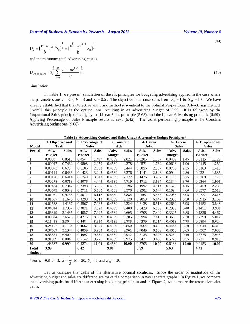
Simulation

In Table 1, we present simulation of the six principles for budgeting advertising applied in the case where

the parameters are a = 0.8, b = 3 and 5.0 . The objective is to raise sales from 10 S to 10MS . We have

already established that the Objective and Task method is identical to the optimal Proportional Advertising method.

Overall, this principle is the optimal one, resulting in an advertising budget of 3.99. It is followed by the

Proportional Sales principle (4.41), by the Linear Sales principle (5.63), and the Linear Advertising principle (5.99).

Applying Percentage of Sales Principle results is next (6.42). The worst performing principle is the Constant

Advertising budget one (9.08).

Table 1: Advertising Outlays and Sales Under Alternative Budget Principles*

Model

1. Objective and

Task

2. Percentage of

Sales

3. Constant

Adv.

4. Linear

Adv.

5. Linear

Sales

6. Proportional

Sales

Period Adv.

Budget

Sales Adv.

Budget

Sales Adv.

Budget

Sales Adv.

Budget

Sales Adv.

Budget

Sales Adv.

Budget

Sales

1 0.0003 0.8518 0.054 1.497 0.4539 2.821 0.0285 1.307 0.0469 1.45 0.0115 1.122

2 0.00047 0.7462 0.0808 2.050 0.4539 4.278 0.0571 1.762 0.0608 1.90 0.0145 1.259

3 0.00073 0.678 0.1106 2.638 0.4539 5.444 0.0856 2.287 0.0765 2.35 0.0183 1.413

4 0.00114 0.6436 0.1423 3.242 0.4539 6.376 0.1141 2.843 0.094 2.80 0.023 1.585

5 0.00178 0.6414 0.1749 3.848 0.4539 7.122 0.1426 3.407 0.1133 3.25 0.0289 1.778

6 0.00278 0.6713 0.2076 4.445 0.4539 7.719 0.1712 3.967 0.1344 3.70 0.0364 1.995

7 0.00434 0.7347 0.2398 5.025 0.4539 8.196 0.1997 4.514 0.1573 4.15 0.0459 2.239

8 0.00679 0.8349 0.2711 5.582 0.4539 8.578 0.2282 5.044 0.182 4.60 0.0577 2.512

9 0.0106 0.9768 0.3012 6.112 0.4539 8.884 0.2567 5.556 0.2085 5.05 0.0727 2.818

10 0.01657 1.1676 0.3298 6.613 0.4539 9.128 0.2853 6.047 0.2368 5.50 0.0915 3.162

11 0.02588 1.4167 0.3567 7.082 0.4539 9.324 0.3138 6.518 0.2669 5.95 0.1152 3.548

12 0.04044 1.7367 0.3821 7.520 0.4539 9.480 0.3423 6.969 0.2988 6.40 0.1451 3.981

13 0.06319 2.1435 0.4057 7.927 0.4539 9.605 0.3708 7.402 0.3325 6.85 0.1826 4.467

14 0.09874 2.6575 0.4276 8.303 0.4539 9.705 0.3994 7.818 0.368 7.30 0.2299 5.012

15 0.15428 3.3044 0.448 8.650 0.4539 9.785 0.4279 8.217 0.4053 7.75 0.2894 5.624

16 0.24107 4.1164 0.4667 8.970 0.4539 9.850 0.4564 8.600 0.4444 8.20 0.3644 6.310

17 0.37667 5.1344 0.4839 9.263 0.4539 9.901 0.4849 8.969 0.4853 8.65 0.4587 7.080

18 0.58854 6.409 0.4997 9.531 0.4539 9.942 0.5135 9.325 0.528 9.10 0.5775 7.943

19 0.91959 8.004 0.5142 9.776 0.4539 9.975 0.542 9.669 0.5725 9.55 0.727 8.913

20 1.43687 9.999 0.5274 10.00 0.4539 10.00 0.5705 10.00 0.6188 10.00 0.9153 10.00

Total

Budget

3.99 6.42 9.08 5.99 5.63 4.41

* For: a = 0.8, b = 3, 2

1 , M = 20, 10 S and 20MS

Let us compare the paths of the alternative optimal solutions. Since the order of magnitude of the

advertising budget and sales are different, we make the comparison in two separate graphs. In Figure 1, we compare

the advertising paths for different advertising budgeting principles and in Figure 2, we compare the respective sales

paths.

1

0

11

01 ][][ S

b

accSc

b

acU

kkk

k



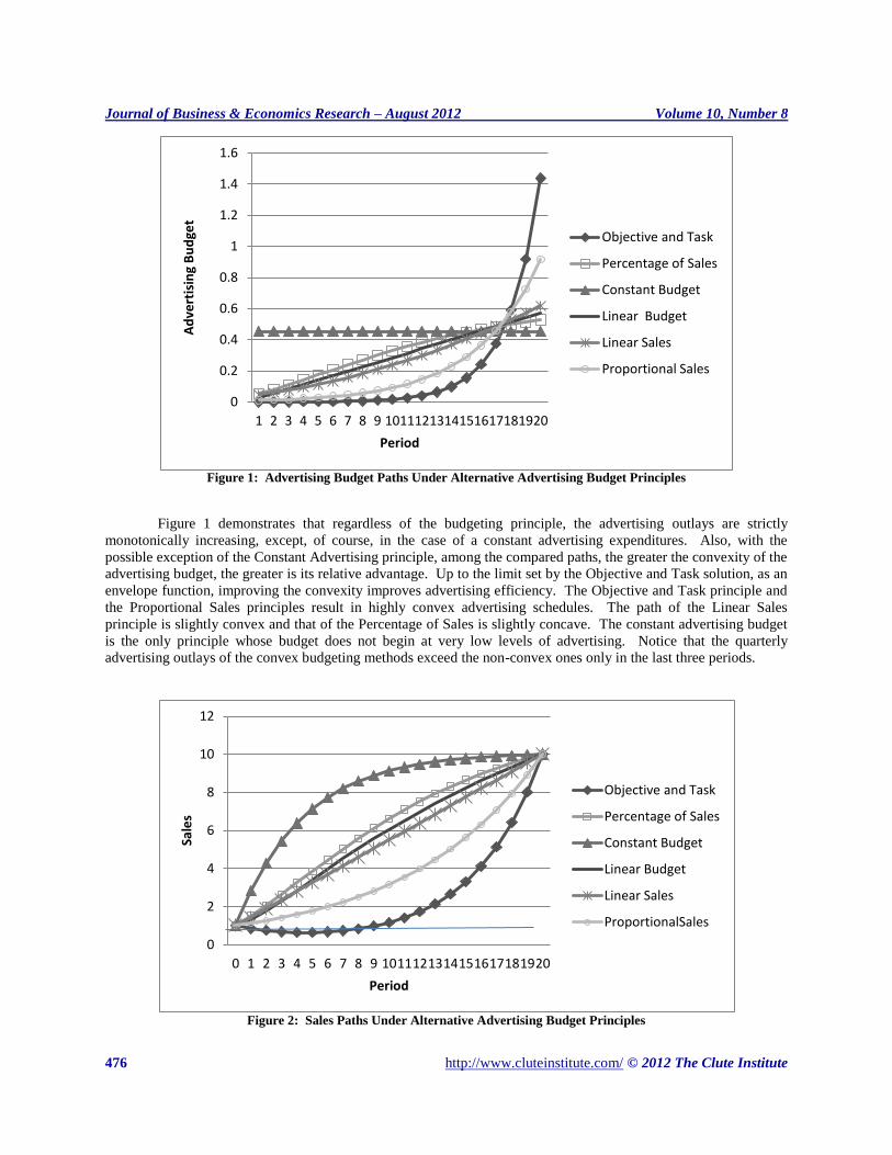
Figure 1: Advertising Budget Paths Under Alternative Advertising Budget Principles

Figure 1 demonstrates that regardless of the budgeting principle, the advertising outlays are strictly

monotonically increasing, except, of course, in the case of a constant advertising expenditures. Also, with the

possible exception of the Constant Advertising principle, among the compared paths, the greater the convexity of the

advertising budget, the greater is its relative advantage. Up to the limit set by the Objective and Task solution, as an

envelope function, improving the convexity improves advertising efficiency. The Objective and Task principle and

the Proportional Sales principles result in highly convex advertising schedules. The path of the Linear Sales

principle is slightly convex and that of the Percentage of Sales is slightly concave. The constant advertising budget

is the only principle whose budget does not begin at very low levels of advertising. Notice that the quarterly

advertising outlays of the convex budgeting methods exceed the non-convex ones only in the last three periods.

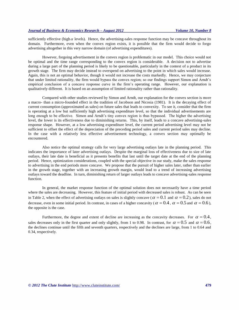
Figure 2: Sales Paths Under Alternative Advertising Budget Principles

0

2

4

6

8

10

12

0 1 2 3 4 5 6 7 8 9 10 11 12 13 14 15 16 17 18 19 20

Sale

s

Period

Objective and Task

Percentage of Sales

Constant Budget

Linear Budget

Linear Sales

ProportionalSales

0

0.2

0.4

0.6

0.8

1

1.2

1.4

1.6

1 2 3 4 5 6 7 8 9 10 11 12 13 14 15 16 17 18 19 20

Ad

vert

isin

g B

ud

get

Period

Objective and Task

Percentage of Sales

Constant Budget

Linear Budget

Linear Sales

Proportional Sales



Figure 2, presenting the sales paths, shows almost uniformly strict sales order that corresponds to the

optimality order of the principles. The only exception is that sales based on Linear Advertising are slightly lower

than those based on Linear Sales in the first three periods. Otherwise, the sales paths of every principle never

intersect and a principle whose sales path is more convex than another corresponds to a lesser total advertising

budget. We can conclude that a higher efficiency in reaching the target is obtained by greater postponement of the

advertising effort to the more distant period. Among the compared principles, the more accelerated the growth in

the sales path at the end of the planning period, the more efficient it is in attaining the target. Like in the case of

advertising path, the Objective and Task sets the limit on this convexity.

THE OPTIMAL OBJECTIVE AND TASK SOLUTION

A close examination of Figure 2 and Table 1 shows that unlike advertising outlays, sales are not necessarily

monotonically increasing, even in the broad sense. Moreover, this exception is important as it applies in the case of

the optimal Objective and Task method. In the first five quarters, its sales are declining and only then turn around

and increase. This indicates that the initial advertising outlays have important noticeable downside. Their impact,

as part of sales increment, is mostly eradicated over time. Their low level and the associated sales decrease is

justified by the need to maximize efficiency in reaching the ultimate sales goal. This need places the focus on

accelerating advertising in the end part of the planning period. Nonetheless, it remains optimal to advertise during

the whole planning period. So, under the objective of the SWC and its dynamics, some advertising is always

preferred over no advertising. In particular, advertising pulsing policies, not considered in this paper, must be

inferior to the Objective and Task solution in this market context.

Consequently, the optimal market response function, of the Objective and Task solution, is qualitatively

different than the traditional ones that exhibit either an S Shape or a convex shape, where sales are always increasing

as advertising budget increases. The Sales response function first increases and then decreases as advertisement

budgets are optimally increase. Figures 3 and 4 represent the market response function for this case.

Figure 3: Optimal (Objective And Task) Sales Response To Advertising For The Whole Planning Period

0

2

4

6

8

10

12

0 0.5 1 1.5 2

Sale

s

Advertising Budget

Sales



Figure 4: Optimal (Objective And Task) Sales Response To Advertising For The First Eight Periods

Based on these findings, we explain the phenomenon of thresholds in advertising effects on sales as a result

of planning and optimization. In contrast, in Hibshoosh (1987) we explain this threshold, alternatively, by the

stochastic character of the attitude and an attitude-behavior threshold. Our findings support two seemingly

contrasting studies. Vakratas, Feinberg, Bass and Kalyanaram (2004) revealed the existence of the advertising-sales

thresholds, that sales response to advertising need not be concave, and that thresholds are likely to be encountered in

the dynamic environment of the earlier stages in the product life cycle. Their study is closely linked with the

arguments for the S-shaped response function of Feinberg (2001) and with Mahajan and Muller’s (1986) treatment

of advertising pulsing strategies.

In contrast, Simon, and Arndt (1980) concluded that the advertising-sales response function, in its

empirically observed section, is concave due to diminishing return. Reviewing the support for concavity and

convexity in the advertising-sales response function, they conceded the existence of a convex region in the initial

region of the advertising sales response function. There was some limited empirical support for this hypothesis, e.g.,

Rao and Miller (1975). The range of the theoretical support for a convex region was wider. It was based primarily

on a functional link between the advertising and intervening psychological variables and, in turn, between those and

sales, which implies the existence of thresholds. Simon and Arndt chose to focus on the following argument for

convexity: At a very low advertising expenditure, the ads are too short to be considered effective. Hence, they

conclude that the convex region would be a very small one and firms would choose not to operate in this convex

region. A similar argument was given by Sasieni (1971) in his analytical qualification of the shape of advertising-

sales response function. However, this conclusion must be understood in its context to avoid logical fallacy. Very

limited advertising expenditure is sufficient for the existence of a convex section. However, it is not a necessary

condition for convexity. The convex region may be wide enough to allow different levels of advertising

expenditures. Hence, Simon and Arndt’s conclusion of a concave response function was ultimately based on the

weight of the empirical evidence.

Our simulation supports the shape conclusion of Simon and Arndt’s while providing a different explanation

for the convexity. In our discrete planning, the convex region does not always exist and when it does, its range is

very narrow and hardly noticeable in first order statistical estimates. It may exist only if the adverting is not

0

0.2

0.4

0.6

0.8

1

1.2

0 0.002 0.004 0.006 0.008

Sale

s

Advertising Budget

Sales



sufficiently effective (high levels). Hence, the advertising-sales response function may be concave throughout its

domain. Furthermore, even when the convex region exists, it is possible that the firm would decide to forgo

advertising altogether in this very narrow domain (of advertising expenditures).

However, forgoing advertisement in the convex region is problematic in our model. This choice would not

be optimal and the time range corresponding to the convex region is considerable. A decision not to advertise

during a large part of the planning period is likely to be questionable, particularly in the context of a product in its

growth stage. The firm may decide instead to overspend on advertising to the point in which sales would increase.

Again, this is not an optimal behavior, though it would not increase the costs markedly. Hence, we may conjecture

that under limited rationality, the firm would bypass the convex region; so our findings support Simon and Arndt’s

empirical conclusion of a concave response curve in the firm’s operating range. However, our explanation is

qualitatively different. It is based on an assumption of limited rationality rather than rationality.

Compared with other studies reviewed by Simon and Arndt, our explanation for the convex section is more

a macro- than a micro-founded effect in the tradition of Jacobson and Nicosia (1981). It is the decaying effect of

current consumption (approximated as sales) on future sales that leads to convexity. To see it, consider that the firm

is operating at a low but sufficiently high advertising expenditure level, so that the individual advertisements are

long enough to be effective. Simon and Arndt’s tiny convex region is thus bypassed. The higher the advertising

level, the lower is its effectiveness due to diminishing returns. This, by itself, leads to a concave advertising-sales

response shape. However, at a low advertising expenditure level, the current period advertising level may not be

sufficient to offset the effect of the depreciation of the preceding period sales and current period sales may decline.

In the case with a relatively less effective advertisement technology, a convex section may optimally be

encountered.

Also notice the optimal strategy calls for very large advertising outlays late in the planning period. This

indicates the importance of later advertising outlays. Despite the marginal loss of effectiveness due to size of late

outlays, their late date is beneficial as it presents benefits that last until the target date at the end of the planning

period. Hence, optimization considerations, coupled with the special objective in our study, make the sales response

to advertising in the end periods more concave. We propose that the pursuit of higher sales later, rather than earlier

in the growth stage, together with an increasing growth margin, would lead to a trend of increasing advertising

outlays toward the deadline. In turn, diminishing return of larger outlays leads to concave advertising-sales response

function.

In general, the market response function of the optimal solution does not necessarily have a time period

where the sales are decreasing. However, this feature of initial period with decreased sales is robust. As can be seen

in Table 2, when the effect of advertising outlays on sales is slightly concave ( 1.0 and 2.0 ), sales do not

decrease, even in some initial period. In contrast, in cases of a higher concavity ( 4.0 , 5.0 and 6.0 ),

the opposite is the case.

Furthermore, the degree and extent of decline are increasing as the concavity decreases. For 4.0 ,

sales decreases only in the first quarter and only slightly, from 1 to 0.98. In contrast, for 5.0 and 6.0 ,

the declines continue until the fifth and seventh quarters, respectively and the declines are large, from 1 to 0.64 and

0.34, respectively.



Table 2: The Effect Of Sales’ Response Concavity On The Optimal Solution*

Alpha Period

0.1

Sales Adv

0.2

Sales Adv

0.4

Sales Adv

0.5

Sales Adv

0.6

Sales Adv

1 1 1 1 1

1 0.00042 2.179 0.00178 1.646 0.00093 0.984 0.00030 0.852 0.00004 0.807

2 0.00054 3.157 0.00235 2.211 0.00135 1.000 0.00047 0.746 0.00008 0.656

3 0.00069 3.975 0.00311 2.714 0.00196 1.048 0.00073 0.678 0.00014 0.539

4 0.00089 4.665 0.00411 3.171 0.00284 1.125 0.00114 0.644 0.00024 0.452

5 0.00114 5.255 0.00543 3.594 0.00411 1.234 0.00178 0.641 0.00042 0.390

6 0.00146 5.765 0.00718 3.992 0.00597 1.374 0.00278 0.671 0.00073 0.351

7 0.00187 6.212 0.00948 4.376 0.00866 1.548 0.00434 0.735 0.00128 0.336

8 0.00239 6.610 0.01253 4.750 0.01256 1.759 0.00679 0.835 0.00223 0.346

9 0.00306 6.970 0.01657 5.121 0.01821 2.011 0.01060 0.977 0.00390 0.384

10 0.00392 7.300 0.02190 5.494 0.02642 2.310 0.01657 1.168 0.00681 0.457

11 0.00503 7.607 0.02894 5.872 0.03832 2.662 0.02589 1.417 0.01189 0.576

12 0.00644 7.897 0.03825 6.260 0.05558 3.074 0.04045 1.737 0.02077 0.754

13 0.00826 8.175 0.05056 6.659 0.08061 3.555 0.06320 2.144 0.03628 1.014

14 0.01058 8.443 0.06683 7.074 0.11693 4.115 0.09875 2.658 0.06339 1.384

15 0.01356 8.706 0.08832 7.505 0.16960 4.768 0.15430 3.305 0.11073 1.908

16 0.01737 8.965 0.11674 7.957 0.24601 5.526 0.24110 4.117 0.19344 2.646

17 0.02226 9.223 0.15430 8.430 0.35684 6.407 0.37672 5.135 0.33793 3.682

18 0.02852 9.480 0.20394 8.927 0.51759 7.431 0.58862 6.409 0.59033 5.132

19 0.03655 9.739 0.26955 9.449 0.75076 8.620 0.91972 8.005 1.03127 7.162

20 0.04683 10.000 0.35626 10.000 1.08898 10.000 1.43707 10.000 1.80155 10.000

Total Adv. 0.21176 1.45812 3.50421 3.99132 4.21344

Total Sales 140.323 115.201 70.551 52.872 38.976

* For: a = 0.8, b = 3, 5.0 , M = 20, 10 S and 20MS .

In our comparison of the optimal solution, we chose to take the case where 5.0 for two reasons. One

reason is that this case, in contrast with others, enables the derivation of explicit analytical solutions using quadratic

terms and equations. It therefore eases exposition. The second, and more important, reason is that results of this

model are both insightful and realistic in the case of products in the growth stage of the product life cycle. Meta

analysis-based study of Sethuraman, Tellis and R. Briesch (2011) suggests a mean elasticity - roughly between 0.1

to 0.2 (.16 for the growth stage) and an elasticity range between 0 and 0.5. However, these estimates are naturally

estimates of the average elasticity of a market response function, and the study reconfirms that average elasticity

varies from one stage of the product life cycle to the next. Since the sales market response is a dynamic process that

depends on past sales and on past advertising outlays, a constant elasticity response, over time, is unlikely to be

realistic, even though it may be a parsimonious approximation of a limit response. In our case, let us emphasize that

concavity parameter is not the elasticity of sales with respect to advertising and the average elasticity varies as a

function of time in our model. Our model, with the parameter 5.0 , makes this point very clear. It has an

initial section of the planning period where advertising increases but sales decline. Hence, calculated elasticities,

using contemporaneous advertising and sales, would be negative in this initial section. On the other hand, at the last

section of a long planning period, we would expect the elasticities to increase toward the 5.0 value, as the size

of the more recent advertising outlay exponentially increase and the effects of the initial sales virtually completely

disappear. In Table 3, we demonstrate that the elasticities are monotonically increasing. They range from -0.220 in

the second period to 0.444 in the final twentieth period. The average elasticity is 0.270 (or 0.259, if estimated by the

ratio of average relative sales change divided by the relative advertising change.). Hence, the average elasticity

described by the reference example of our model, with 5.0 , is not unrealistic, particularly for products in the

growth stage of the product life cycle in fast expanding industries.



Table 3: Contemporaneous Sales Advertising Elasticities*

Period Adv. Dadv./Adv Sales Dsales/Sales Elasticity

1 0.00030 0.85183 -0.14817

2 0.00047 0.56250 0.74625 -0.12395 -0.22035

3 0.00073 0.56250 0.67798 -0.09148 -0.16263

4 0.00114 0.56250 0.64361 -0.05069 -0.09012

5 0.00178 0.56250 0.64142 -0.00340 -0.00604

6 0.00278 0.56250 0.67131 0.04659 0.08283

7 0.00434 0.56250 0.73476 0.09452 0.16803

8 0.00679 0.56250 0.83494 0.13635 0.24241

9 0.01060 0.56250 0.97688 0.16999 0.30221

10 0.01657 0.56250 1.16766 0.19529 0.34719

11 0.02589 0.56250 1.41682 0.21339 0.37935

12 0.04045 0.56250 1.73682 0.22586 0.40153

13 0.06320 0.56250 2.14366 0.23425 0.41644

14 0.09875 0.56250 2.65768 0.23979 0.42629

15 0.15430 0.56250 3.30459 0.24341 0.43273

16 0.24110 0.56250 4.11673 0.24576 0.43691

17 0.37672 0.56250 5.13471 0.24728 0.43960

18 0.58862 0.56250 6.40942 0.24825 0.44134

19 0.91972 0.56250 8.00460 0.24888 0.44245

20 1.43707 0.56250 10.00001 0.24928 0.44317

Average 0.56250 0.14576 0.27072

* For: a = 0.8, b = 3, 5.0 , M = 20, 10 S and 20MS .

CONCLUDING REMARKS AND DIRECTIONS FOR FUTURE RESEARCH

In this paper, we characterized sales response to advertising for a firm that is effectively marketing its

product in a fast-growing industry in the introduction or early growth stage. The firm’s objective is to efficiently

attain a minimal sales level within a pre-specified planning period. We modeled the problem as a SWC problem

augmented with some alternative basic regularity conditions placed either on the sales path or on the advertising

budget path.

Advertising may not be the preferred mode of promotion in many circumstances in the introductory and

growth stages and its specific nature and purpose usually change as the product sales grow. However, many firms

keep allocating marketing resources to advertising for the ultimate purpose of sales increase, and advertising budgets

are, in practice, strongly linked with the firm’s sales level and regularity conditions

We found that regardless of whether the regularity requirements are initially placed on the sales or on

advertising, both corresponding paths, and thus also the sales response to advertising, exhibit regularity. We showed

that the regularity conditions uniquely determine the paths and derived explicit optimal path solutions.

Our derivation of parametric explicit solutions and recursive functional relationship for optimal advertising

and sales under different regularity conditions facilitate both insight into the advertising and sales processes as well

as easy computation and simulation of their optimal paths.

We found that a path’s regularity conditions create a mechanism that induces a degree of convexity (or

concavity) on the corresponding paths and thus shapes them. In particular, the degree of this convexity for the

advertising path determines the relative efficiency of its budgeting principle. The optimal advertising and sales

paths of the SWC turned out to be highly convex and sets the limit on the optimal convexity.

Our finding helps explain the inconsistency in reported values of advertising elasticities and the

phenomenon of thresholds in the effectiveness of advertising. We demonstrated that when the “technology” of sales

production by advertising is relatively inefficient, employing the optimal advertising plan may require acceptance of

sales decrease and thus negative elasticities while advertising outlays are accelerated.



Our inquiry can be advanced in several directions. First, modeling based on combining extant

mathematical extensions of the SWC, with observations drawn from marketing and business practices, would

increase the range of validity of SWC-based modeling. For example, marketing adaptation of the ideas in Chen

(1991) and Lee and Leitmann (1991) would enable analysis of advertising decisions for old products in their

maturity stage. Likewise, incorporating various boundary conditions, commonly offered by scholars extending the

SWC, would help modeling advertising budgeting under capital budgeting conditions. Second, incorporating

additional selective elements of the marketing mix and their relationship would result in more comprehensive

models for the introduction and growth stages of the product life cycle. These elements would include availability,

price, strategic product modifications, and their relationships. Third, considering market structure effects, through

embedding the SWC dynamics within a game theoretical framework, would clarify options in competitive strategy

and facilitate welfare comparisons.

These extension efforts would help improve our advertising budgeting process, in particular, and advance

our knowledge of the functioning of promotion as a tool of dynamic demand management in business and

economics.

AUTHOR INFORMATION

Aharon Hibshoosh is a professor in the department of Marketing and Decision Sciences at the College of Business

at San Jose State University. He received his PhD from the School of Business at UC Berkeley in 1974. His area

of research is modeling the intersection of Marketing with Economics, Statistics and Mathematics. He also taught at

UC Berkeley, CUNY’s Baruch College, and The Hebrew University. He served as a consultant for major public

institutions and private firms. He published in the Journal of Marketing Research, Mathematical Modeling,

Decision Sciences, the International Journal of the Economics of Business, and others. E-mail:

[email protected]

REFERENCES

1. Buratto, A., & Viscolani, B. (1994). An Optimal Control Student Work Problem and a Marketing

Counterpart. Mathematical and Computer Modelling, 20 (6), 19-33.

2. Chen Y.H. (1991). A Revisit to the Student Learning Problem. Optimal Control Applications and Methods,

12 (4), 263-272.

3. Feinberg F.M. (2001). On Continuous-Time Optimal Advertising under S-Shaped Response. Management

Science, 47 (11), 1476-1487.

4. Hibshoosh, A. (1987). Attitude Distribution Change as a Marketing Approach to Action/Sales

Maximization. Mathematical Modeling, 8, 670-673.

5. Jacobson R. & Nicosia F. M. (1981). Advertising and Public Policy: The Macro Economics Effects of

Advertising. Journal of Marketing Research, 18, 29-38.

6. Klamkin, M.S. (1985). Mathematical Modeling: a Student Optimal Control Problem and Extensions.

Mathematical Modeling, 6 (1), 49-64.

7. Lee C.S. & Leitmann G.L. (1991). Some Stabilizing Study Strategies for a Student-Related Problem under

Uncetainty. Dynamics and Stability of Systems, 6 (1), 63-78.

8. Low, G. S. & Mohr, J. J. (1999). Setting Advertising and Promotion Budgets in Multi-Brand Companies.

Journal of Advertising Research, 39 (1), 67-78.

9. Mahajan,V.E. & Muller.E. (1986). Advertising Pulsing Policies for Generating awareness for New

Products, Marketing Science, 52 (2), 89-106.

10. Miller, N. & Pazgal, A.(2007). Advertising Budget in Competitive Environment. Quantitative Marketing

and Economics, 5 (2), 131-161.

11. Mitchell, L. A. (1993). An Examination of Methods of Setting Advertising Budgets: Practice and the

Literature., European Journal of Marketing, 27 (5) , 5-22.

12. Nerlove, M. & Arrow, K.J. (1962). Optimal Advertising Policy under Dynamic Conditions. Economica,

29, 129-42.

13. Raggett, G.F., Hempson, P.W. & Jukes, K.A. (1981). A student related optimal control problem. Bulletin

of The Institute of Mathematics and its Applications, 17, 133-136 (1981).

http://search.proquest.com.libaccess.sjlibrary.org/docview.lateralsearchlink:lateralsearch/author/Mitchell,+Lionel+A/$N?site=abicomplete&t:ac=237007821/12D8D21478E4A55B3BA/6&t:cp=maintain/resultcitationblocks

http://search.proquest.com.libaccess.sjlibrary.org/docview.lateralsearchlink_1:lateralsearch/pubtitle/European+Journal+of+Marketing/$N/3659?site=abicomplete&t:ac=237007821/12D8D21478E4A55B3BA/6&t:cp=maintain/resultcitationblocks

http://search.proquest.com.libaccess.sjlibrary.org/docview.issuebrowselink:searchpublicationissue/3659/European+Journal+of+Marketing/01993Y01Y01$231993$3b++Vol.+27+$285$29/27/5?site=abicomplete&t:ac=237007821/12D8D21478E4A55B3BA/6&t:cp=maintain/resultcitationblocks



14. Rao, A.G., and Miller, P.B. (1975). Advertising/Sales Response Functions. Journal of Advertising

Research, 15 (2), 1-15.

15. Sasieni, M.W. (1971). Optimal Advertising expenditures. Management Science, (18), 64-72.

16. Simon J. L. & Arndt. J. (1980). The Shape of the Advertising Response Function. Journal of Advertising

Research, 20 (4), 11-28.

17. Sethuraman, R., Tellis, G.J. & Briesch R. (2011). How Well Does Advertising Work? Generalization from

a Meta-Analysis of Brand Advertising Elasticity. Forthcoming Journal of Marketing Research,

Forthcoming.

18. Vakratas, D., Feinberg, F. M., Bass F. M. &, Kalyanaram G. (2004). The Shape of Advertising Response

Functions Revisited: A Model of Dynamic Probabilistic Thresholds. Marketing Science, 23 (-1), 109-119.

19. Vidalle, M. L. & Wolfe H.B. (1957). An Operations Research Study of Sales Response to Advertising.

Operations research, 5 (3), 370-381.

20. Vornicescu N. (2009). A Problem in Non Linear Optimization. Journal of Science and Art, 9 (1), 71-75.

21. Wagner, N. (2011). A Descriptive and Normative Analysis of Marketing Budgeting (Unpublished Doctoral

Dissertation), University of Cologne, Germany.

22. Yoo, B. & Mandhachitara, R. (2003). Estimating Advertising Effects of Sales in a Competitive Setting.

Journal of Advertising Research, 43 (3), 310- 321.

http://search.proquest.com.libaccess.sjlibrary.org/abicomplete/docview/212240745/136C38A4CA815B680A7/3?accountid=10361

http://search.proquest.com.libaccess.sjlibrary.org/abicomplete/docview/212240745/136C38A4CA815B680A7/3?accountid=10361



NOTES

Documents

Advertising Budget And Sales Paths Under The Dynamics Of