ADVERTISING, BRAND LOYALTY AND PRICING*

Ioana Chioveanu**

WP-AD 2005-32 Editor: Instituto Valenciano de Investigaciones Económicas, S.A. Primera Edición Noviembre 2005 Depósito Legal: V-4678-2005 IVIE working papers offer in advance the results of economic research under way in order to encourage a discussion process before sending them to scientific journals for their final publication.

* I would like to thank Xavier Vives, as well as Ugur Akgun, Ramon Caminal, Xavier Martinez, Pierre Regibeau, and an anonymous IVIE referee for very helpful comments. The paper benefited from comments of participants to UAB Micro Workshop, EEA, EARIE, ASSET and SAE Meetings (2003). Any remaining errors are mine. ** I. Chioveanu: Economics Dept., University of Alicante, Campus San Vicente, E-03071, Alicante, Spain, email: ioana@merlin.fae.ua.es.

2

ADVERTISING, BRAND LOYALTY AND PRICING

Ioana Chioveanu

ABSTRACT

I construct a model in which an oligopoly first invests in persuasive advertising in order

to induce brand loyalty to consumers who would otherwise buy the cheapest alternative on

the market, and then competes in prices. Despite ex-ante symmetry, at equilibrium, there is

one firm which chooses a lower advertising level, while the remaining ones choose the same

higher advertising. For the endogenous profile of advertising expenditure, there are a family

of pricing equilibria with at least two firms randomizing on prices. The setting offers a way

of modelling homogenous product markets where persuasive advertising creates subjective

product differentiation and changes the nature of subsequent price competition. The pricing

stage of the model can be regarded as a variant of the Model of Sales by Varian (1980) and

the two stage game as a way to endogenize consumers heterogeneity raising a robustness

question to Varian’s symmetric setting.

Keywords: oligopoly, advertising, price dispersion, brand loyalty

JEL: D21, D43, L11, L13, M37

1 Introduction

The interest in the economic analysis of advertising is continuously resuscitated by the amazing

diversity of media1 and by the large amounts invested in advertising. The US 100 largest

advertisers spent a total of USD 90.31 billion on advertising in 2003, with amounts ranging

between USD 0.317-3.43 billions.2 The most advertised segments include many consumer goods:

Beer, cigarettes, cleaners, food products, personal care, and soft drinks. In many of these

markets the goods are nearly homogenous, and eventually advertising, rather than increasing

the demand, redistributes the buyers among sellers.

In the present paper, I study the strategic effect of persuasive advertising in homogenous

product markets. For this purpose, I construct a model of two-dimensional competition in

non-price advertising and prices. Firms first invest in advertising in order to induce brand

loyalty to consumers who would otherwise purchase the cheapest alternative on the market,

and then compete in prices for the remaining brand indifferent consumers. At equilibrium,

prices exhibit dispersion being random draws from asymmetric distributions. The variation in

the price distributions is reflected by the expected profits and, in consequence, the advertising

levels chosen by the firms are asymmetric. There is one firm choosing a lower advertising level,

while the remaining firms choose the same higher advertising. For this profile of advertising

expenditure, there are a family of pricing equilibria with at least two firms randomizing on

prices. One limiting equilibrium has all firms randomizing; the other one has only two firms

randomizing and the others choosing monopoly pricing with probability 1. As the number of

rivals increases, more firms prefer to price less aggressively, counting on their loyal bases rather

than undercutting in order to capture the indifferent market. In this model the low advertiser

1Magazines, newspapers, television, radio, internet or outdoor ads.2Advertising Age, June 28, 2004, 100 Leading National Advertisers.

3

prices more aggressively, while the heavy advertisers’ expected prices are higher. The firms are

counterbalacing their advertising and pricing decisions.

The setting proposes a way of modelling homogenous product markets where persuasive ad-

vertising creates subjective product differentiation and changes the nature of subsequent price

competition. It also offers a new perspective on the coexistence of advertising and price dis-

persion. The market outcome turns out to be asymmetric, despite a priori symmetry of the

firms.

The prediction of an asymmetric advertising expenditure profile may be more adequate for

small oligopolies. The results relate to the carbonated cola drinks market in the US, where

Coca Cola and Pepsico invest similar large amounts in advertising, while Cadbury-Schweppes

has lower advertising expenditure. Similarly, in the US sport drinks market, Pepsico highly

advertises its product Gatorade, while Coca Cola promotes less its product Powerade.

The persuasive view on advertising goes back to Kaldor (1950).3 More recently, Friedman

(1983) and Schmalensee (1972,1976) dealt with oligopoly competition in models where adver-

tising increases selective demand.4 Schmalensee (1972) explores the role played by promotional

competition in differentiated oligopoly markets where price changes are infrequent. This article

departs from his work assuming that competition takes place in both advertising and prices.

Much empirical work explored whether homogenous goods advertising is informative and

affects the primary (industry) demand, or is persuasive and affects only the selective (brand)

demand. The results are often contradictory, and they seem to vary across industries. The

3Robinson (1933), Braithwaite (1928), Galbraith (1958, 1967) and Packard (1957,1969) also contributed to

this view.4Von der Fehr and Stevik (1998) and Bloch and Manceau (1999) analyze the role of persuasive advertising

in differentiated duopoly markets, and Tremblay and Polasky (2002) show how persuasive advertising may affect

price competition in a duopoly with no real product differentiation.

4

persuasive view was supported by Baltagi and Levin (1986) in the US cigarette industry, and

by Kelton and Kelton (1982) for US brewery industry. Using inter-industry data, they report

a strong effect of advertising on selective demand.5 More recent studies, using disaggregated

data (at industry or brand level), show that advertising is meant to decrease consumers’ price

sensitivity. For instance, Krishnamurthi and Raj (1985) find that brand demand becomes more

inelastic once advertising increases.6

In a model where advertising creates vertical differentiation, Sutton (1991) points out to

the existence of two-tier markets as a result of differences in consumer tastes.7 In his study,

frozen-food industry illustrates the emergence of dual structures (where high-advertisers coexist

with nonadvertisers) in advertising-intensive markets. As in Sutton’s model post advertising

consumers tastes are heterogenous here.8 However in my model not all consumers rank the

advertised products the same (advertising induces subjective "horizontal differentiation"), and

the number of advertising-responsive consumers is endogenous. I show that a dual structure

emerges though the indifferent consumer and the loyal markets are not independent.

Although it takes a different view on advertising, this article shares a number of technical

features with part of the informative advertising literature dealing with price dispersion phe-

nomena. A seminal article by Stigler (1961) revealed the role of informative advertising in

5Lee and Tremblay (1992) find no evidence that advertising promotes beer consumption in the US. Nelson and

Moran (1995), in an inter-industry study of alcoholic beverages, conclude that advertising serves to reallocate

brand sales.6Pedrick and Zufryden (1991) report a strong direct effect of advertising exposure over brand choice in the

yogurt industry. However, some recent empirics point out towards the dominance of experience over advertising.

See Bagwell (2003) for a review.7He focuses on the concentration-market size relationship in industries where firms incur endogeneous sunk

costs, and contrasts these results with those in markets with exogeneous setup costs.8 In his setting, nonretail buyers do not respond to advertising, unlike retail customers.

5

homogenous product markets, and related it to price dispersion.9,10

The pricing stage of the game can be viewed as a modified version of the model of sales by

Varian (1980), in the sense that the total base of captured consumers is shared asymmetrically

instead of being evenly split among the firms. The two-stage game offers a way of endogeneizing

consumers’ heterogeneity: It turns out that the symmetric outcome does not obtain, raising a

robustness question to Varian’s (1980) symmetric model.

Baye, Kovenock and de Vrier (1992) present an alternative way of checking the robustness

of Varian’s symmetric setting. They construct a metagame where both firms and consumers are

players, and asymmetric price distributions cannot form part of a subgame perfect equilibrium.

In my model, only firms are making decisions and the subgame perfect equilibria of the game

are asymmetric.

Narasimhan (1988) derived the mixed pricing equilibrium in a price-promotions model where

two brands act as monopolists on loyal consumer markets and compete in a common market

of brand switchers. The pricing stage of my model extends his setting to oligopoly, when the

switchers are extremely price sensitive.

Section 2 describes the model, while section 3 derives the equilibrium in the pricing stage.

Section 4 presents the equilibrium emerging in the advertising stage, and defines the outcome of

the sequential game. Sections 5 and 6 discuss the setting and present some concluding remarks.

All the proofs missing from the text are relegated to an Appendix.

9Butters (1977), Grossman and Shapiro (1984), McAfee (1994), Robert and Stahl (1993), Roy (2000) construct

price dispersion models where oligopolists use targeted advertising to offer information about their products to

consumers who are completely uninformed or incur costly search to collect information.10Recently, clearinghouse models have been used to explain persistent price dispersion in internet markets,

see Baye and Morgan (2001). The present setting can be linked to virtual markets: in the presence of price-

comparison sites, firms have incentives to engage (prior to price competition) in costly search frustration activities

(obfuscation). See Ellison and Ellison (2001).

6

2 The Model

There are n firms selling a homogenous product. All firms have the same constant marginal cost.

In the first period, firms choose simultaneously and independently an advertising expenditure

and, in the second period, they compete in prices. Let αi be the advertising expenditure chosen

by firm i.

This model deals with non-price advertising. Each firm promotes its product to induce

subjective differentiation and generate brand loyalty.11 The fraction of consumers that are loyal

to firm i depends on the advertising expenditure profile. At the end of the first stage, the

advertising choices become common knowledge.

In the second stage, firm i chooses the set of prices that are assigned positive density in

equilibrium and the corresponding density function. Let Fi (p) be the cumulative distribution

function of firm i’s offered prices. The price charged by a firm is a draw from its price distribution.

I assume that there is a continuum of consumers, with total measure 1, who desire to

purchase one unit of the good whenever its price does not exceed a common reservation value

r. After advertising takes place, part of the consumers remain indifferent (possibly because no

advertising reached them or, alternatively, no advertising convinced them) and the remaining

ones become loyal to one brand or another. The indifferent consumers view the alternatives on

the market as perfect substitutes and all purchase from the lowest price firm. The size of each

group is determined by the total advertising investment in the market. The total number of

loyal consumers, U, is assumed to be a strictly increasing and concave function of the aggregate

advertising expenditure of the firms, U = U (Σiαi) , with limΣiαi→∞

U (Σiαi) = 1.12 Thus, with

11Advertising may carry some emotional content that potentially touches people and makes them develop loyalty

feelings for the product. Although there is no real differentiation among the products due to advertising they

elicit different associations. See Section 5 for a more detailed discussion on this view.12The empirical studies often present evidence that advertising is subject to diminishing returns to scale. See

7

higher advertising more consumers join the captured (loyal) group. One may think that more

advertising would be more convincing. The captured consumers are split amongst the firms

according to a market sharing function depending on the advertising expenditure of the firms.13

Let it be Si (αi, α−i) = Si ∈ [0, 1], satisfying the following properties:14

1.nPi=1

Si = 1;

2.∂Si∂αi≥ 0 with strict inequality if ∃j 6= i s.t. αj > 0 or if αj = 0, for all j;

3.∂Si∂αj

≤ 0 with strict inequality if αi > 0;

4. Si (αi, 0) = 1 if αi > 0;

5. Si (0, α−i) = 0 if ∃j 6= i s.t. αj > 0 and S (0, 0) = 0;

6. Si (αi, α−i) is homogeneous of degree 0;

7. Si (α, α−i) = Sj (α, α−j) , ∀i, j ∈ N, whenever α−j is obtained from α−i by permutation.

Conditions 1, 4 and 5 require that all loyal consumers be split amongst the firms with positive

advertising expenditure. Conditions 2 and 3 require that a higher own advertising increase the

market share of a firm, whenever it is below 1, and a higher rival advertising decrease the share

of a firm whenever it is above 0. Condition 6 requires that the share profile remain unchanged

to multiplications of the advertising by the same factor.15 Condition 7 states that the market

the reviews by Scherer and Ross (1990) and Bagwell (2003).13 I model captured consumers as a share of total loyals. Alternatively, one can directly define the loyal base

of firm i as Ui (αi, α−i) ≥ 0, satisfying the appropriate assumptions. (See Section 4 for more details.) Then,

U =Pi

Ui (αi, α−i) < 1 should hold.14This function is used by Schmalensee (1976). An example of loyal market share function satisfying these

conditions is S (αi, α−i) =αai

Σjαaj, a > 0.

15However, for instance, doubling the advertising expenditure leads to an increase in the size of the loyal market,

although the sharing rule does not change. Hence, escaladating advertising would increase the captured base of

8

share of a firm is determined by the rivals’ advertising levels and not by their identity. The

symmetry of the loyal market sharing function follows from the symmetry of the firms.

Finally, the remaining consumers form the base of indifferent consumers, denominated by

I. Hence, each firm faces an indifferent base I = 1 − U (Σiαi) and a particular captured or

locked-in base Ui = Si (αi, α−i)U (Σiαi) . Firms cannot price discriminate between these two

types of consumers.16

The timing of the game can be justified by the fact that I deal with non-price advertising.

Firms are building-up a brand identity through advertising expenditure. A change in the brand

advertising takes time, whereas firms can modify their prices almost continuously.

The subgame perfect Nash equilibrium is derived by solving backwards the two stage advertising-

pricing game.

3 The Pricing Stage

In the first stage, firms simultaneously choose the advertising investments. In the second stage,

knowing the whole profile of advertising expenditure, firms choose prices. In this section I solve

the pricing game for an arbitrary weakly ordered profile of advertising expenditure. Let Ui be

the loyal base of consumers captured by firm i, and let I = 1− U = 1−nPi=1

Ui be the group of

brand switchers who buy the lowest priced brand. Without loss of generality, assume Ui ≥ Uj

whenever i ≤ j with i, j ∈ N = {1, 2, ...n}.17

For any firm i ∈ N only the prices in the interval Ai = [c, r] are relevant, with c being the

each firm, all else equal.16Post advertising, some consumers face infinite costs of switching from their favorite brand to another, while

the others have no switching costs. Persuasive advertising induces a psychological switching cost.17Loyal consumers buy their favourite brand whenever its price does not exceed their reservation value. To

characterize the off-the-equilibrium path, assume that, in case their favourite is priced above the reservation value,

loyals purchase a random product whenever is priced below reservation value.

9

common constant marginal cost of production. Pricing at pi < c firms would make negative

profits and pricing at pi > r firms would make zero profits.

The profit function of firm i, i = 1, 2...n is given by:

πi (pi, p−i) =

(pi − c) (Ui + Iφ) if pi ≤ r and pi < pk,∀k ∈ NÂT

with T = {j ∈ N | pi = pj} and φ = 1|T | ;

(pi − c)Ui if pi ≤ r and ∃j 6= i s.t. pj < pi.

(1)

The firms choose the prices that maximize their payoffs taking as given the pricing strategies of

the rivals.

At this stage, firms count with a loyal group and at the same time they compete for the

remaining brand indifferent consumers. However, if all firms price above marginal costs, there

are incentives to undercut in order to win the switchers market. Pricing at marginal cost cannot

form part of an equilibrium as firms can always obtain monopoly profits on their loyal base. The

tension between the incentives to undercut in order to win the indifferent market and those to

extract surplus from the loyals lead to the following result.

Proposition 1 The game (Ai, πi; i ∈ N) has no pure strategy Bertrand-Nash equilibrium.

Existence of a mixed strategy equilibrium can be proven by construction.18 This approach

gives also the functional forms of the equilibrium pricing strategies of the firms.

A mixed strategy for firm i is defined by a function, fi : Ai → [0, 1] , which assigns a

probability density fi (p) ≥ 0 to each pure strategy p ∈ Ai such thatRAifi (p) dp = 1.

Let bSi be the support of the equilibrium price distribution of firm i and [Li,Hi] its convex

hull. This means that fi (p) > 0 for all p ∈ bSi. Denominate by Fi (p) the cumulative distribution18 It is guaranteed as the pricing game satisfies the conditions found by Dasgupta and Maskin (1986, p. 14,

Thm.5). The emergence of mixed-strategy equilibria when there is a mass of consumers with zero switching costs

and there are consumers with positive switching costs was also pointed out by Klemperer (1987).

10

function related to fi (p) . Let limε→0Fj (p)− Fj (p− ε) = PFj (p) .

At a price p, a firm sells to its loyal market and is the winner of the indifferent market

provided that p is the lowest price. Consequently, its expected demand is given by:

Di (p) = (1− ΣiUi)ϕi (p) + Ui where

ϕi (p) =n−1Xk=0

1

1 + k

XM⊆N−i|M |=k

[nQ

j=1j∈M

PFj (p)nQl=1l /∈M

(1− Fl (p))] with N−i = N\ {i} .

The following lemmas present a number of features of the price distributions. The lowest

bound of the price supports has to be shared by at least two firms. If only one firm puts

positive density on the minimal lower bound, this firm has incentives to move the density to the

second lowest bound. In-between the two prices, the firm faces no competition and its profits

are increasing. There exists a (low) price at which selling to its maximal market (loyal group

plus the switchers) a firm makes profits equal to monopoly profits on its loyal base. A firm does

not put positive density at prices below this specific level. At any price in its support a firm

faces a positive probability of loosing the switchers. Hence all firms put positive density on the

monopoly price. If all firms have an atom at the upper bound, there is a positive probability of

a tie and, therefore, (unilateral) incentives to undercut. An analogous reasoning indicates that

the distribution function should be continuos below the upper bound.

Lemma 1 Let L = Lk = mini {Li} . Then ∃ j 6= k, such that Lj = Lk = L. Moreover for each

firm

Li − c ≥ (r − c)Ui

Ui + I.

Proof. If Lk = mini∈N

{Li} and @ j, s.t. Lj = Lk, choosing a lower bound in the interval

(Lk, L0) , with L0 = min

i6=k{Li} , does not decrease firm k’s probability of being the winner of

the indifferent consumers, and strictly increases its expected profits. Then, ∃ j 6= k, such that

11

Lj = Lk. Suppose firm i chooses a price p such that p − c < (r − c) UiUi+I

. Then, the maximal

profits of firm i when pricing at p are (p− c) (I + Ui) < (r − c)Ui. The RHS represents the

guaranteed profit of firm i when it sells only to its loyal base at the monopoly price (its minmax

value). Then, Li − c ≥ (r − c) UiUi+I

for all i.

Lemma 2 Hi = r, ∀ i ∈ N.

Proof. At any price pi > r, πi (pi, p−i) = 0. This implies Hi ≤ r. Let Hm = mini∈N

{Hi}.

Suppose by contradiction that Hm < r.

I show first that (a) @j ∈ N such that Fj (r−) − Fj (Hm) > 0. Suppose such j existed. Since

Fm (p) = 1 and πj (p) = (p− c)Uj < (r − c)Uj for p ∈ (Hm, r), firm j would have a unilateral

profitable deviation choosing instead eFj such that eFj (p) = Fj (p) for p ≤ Hm and P eFj (r) =1− Fj (Hm) . The gain in profit is (r − c)UjP eFj (r)− R rHm

(p− c)UjdFj − (r − c)UjPFj (r) > 0.

To complete the proof I show that (b) A = {i ∈ N | Hi = Hm} = ∅. (By (a), Hj = r for

j ∈ N \A.)

(b1) Assume PFj (Hm) > 0 for ∀j ∈ A. If |A| > 1 or if |A| = 1 and PFk (Hm) > 0 for some

k ∈ NÂA, then there is positive probability of a tie and firm i ∈ A is better off moving PFi (Hm)

to Hm − δ for some δ > 0. If |A| = 1 (⇔ A = {m}) and PFj (Hm) = 0 for ∀j ∈ N−m, then

∃δ > 0 such that ∀p ∈ (Hm − δ,Hm) , (p− c) (Um + Iϕm (p)) < (r − c− ε) (Um + Iϕm (r − ε)),

and firm m would deviate to eFm such that eFm (p) = Fm (p) for p ≤ Hm − δ and P eFm (r − ε) =

Fj (Hm)− Fj (Hm − δ).

(b2) Assume PFj (Hm) = 0, ∀j ∈ N. Since ϕi (Hm) = ϕi (r − ε) = 0, it follows that ∃ε > 0 such

that (Hm − c)Ui < (r − ε− c)Ui for i ∈ A. As before firm i has incentives to deviate.

(b3) ∃j ∈ N, j 6= m such that PFj (Hm) = 0. The argument in (b2) applies.

It follows from (b1)-(b3) that A = ∅.

12

Lemma 3 There is at least one firm that does not have an atom at r.

Proof. Assume to the contrary that PFi (r) > 0 for all i. Consider firm k: ∃ε such that

(r − c) (Uk + Iϕi (r)) < (r − c− ε) (Uk + Iϕi (r − ε)) . Let eF εk be the sequence of unilateral de-

viations defined by eF εk (p) = Fk (p) for p < r − ε and eF ε

k (r − ε) = 1. Firm k has a unilateral

profitable deviation as limε→0+

[πk

³ eF εk , F−k

´− πk (Fk, F−k)] = (r − c) I (n− 1)ϕk (r)PFk (r) > 0.

Lemma 4 Fi (p) is continuous on [Li, r).

Proof. A heuristic proof follows, and a formal one is presented in the Appendix. If firm i

has a jump at p ∈ [Li, r), then ∃ε > 0 such that for j 6= i, Fj (p) = Fj (p+ ε) . Otherwise, firm j

would increase its expected profit by choosing p− δ, instead of pj ∈ (p, p+ ε). This contradicts

the optimality of p given that firm i would only increase its profits by moving the mass to p+ ε.

Notice that this argument fails at p = r because profits at r + ε are equal to zero.

Remark 1 In continuation I restrict attention to equilibria with convex supports. Notice that

Lemmas 1-4 do not rule out the existence of degenerate distributions for some firms.

I propose the following asymmetric pricing equilibrium, valid for any weakly ordered profile

of loyal bases.

Conjecture 1 For U1 ≥ ... ≥ Un−1 ≥ Un, there is an equilibrium with supports bSn = [L, r] ,

bSn−1 = [L, r] and bSk = {r} for k ≤ n − 2. The cdf’s Fn (p) and Fn−1 (p) are continuous on

[Li, r) and PFn−1 (r) > 0.

Note that by Lemma 1, Li − c ≥ (r − c) UiI+Ui

for all i and L− c ≥ (r − c) Un−1I+Un−1 .

Assuming convex supports, Lemma 4 implies that πn (p) = (p− c)

"IQi6=n(1− Fi (p)) + Un

#

and πn−1 (p) = (p− c)

"IQ

i 6=n−1(1− Fi (p)) + Un−1

#are constant on [L, r). Then, necessary

13

conditions for the equilibrium are

πn (L) = (L− c) (I + Un) = πn (r−) = (r − c)

ÃIQi6=n(1− Fi (r

−)) + Un

!;

πn−1 (L) = (L− c) (I + Un−1) = πn−1 (r−) = (r − c)

ÃIQ

i6=n−1(1− Fi (r

−)) + Un−1

!.

By Lemma 3, ∃j ∈ N such that PFj (r) = 0. Suppose n 6= j and PFn (r) 6= 0.

Then πn (r) = (r − c)Un. The first necessary condition implies that L − c = (r − c) UnI+Un

.

But L− c ≥ (r − c) Un−1I+Un−1 . This is only true if Un−1 = Un.

For Un−1 > Un I reached a contradiction. PFn (r) = 0 must hold. Hence the second necessary

condition implies that L− c = (r − c) Un−1I+Un−1 and PFn−1 (r) =

Un−1−UnUn−1+I .

If Un−1 = Un, there are two cases: a. PFn−1 (r) 6= 0. It can be shown that this cannot form

part of an equilibrium19; b. PFn−1 (r) = 0. But then it follows that PFn (r) =Un−Un−1Un+I

= 0. A

contradiction.

Therefore, PFn (r) = 0 and L = (r − c) Un−1I+Un−1 + c (also PFn−1 (r) =

Un−1−UnUn−1+I ).

At equilibrium a firm should be indifferent among all the strategies (prices) that form the

support of its distribution function. Firm n should be indifferent between any price p ∈ [L, r)

and pricing at the lower bound of its support, L. It follows that:

(p− c) [(1− Fn−1 (p)) I + Un] = (L− c) (I + Un)⇒

Fn−1 (p) =(p− L) (Un + I)

I (p− c).

Similarly, firm n− 1 should be indifferent between any price p ∈ [L, r) and pricing at the upper19Consider a simple example with n = 3 and c = 0. Let U1 ≥ U2 = U3. In this case we would have

PF3 (r) > 0, PF2 (r) > 0, and PF1 (r) = 0. Since Li = min bSi and L1 ≥ L2 = L3, F1 (L1) = 0. No-

tice that on [L3, L1) , 1 − F2 (p) = 1 − F3 (p) =(r−p)U3

pI. The constant profit conditions on [L1, r) and

Lemma 4 imply that (1− F2 (p))2 =

(L1−p)U1L1I+(r−L1)2U23pL1I2

. But this implies that (1− F2 (r))2 = (PF2 (r))

2 =

(L1−r)U1L1I+(r−L1)2U23rL1I2

=(L1−r)[U1L1I+(L1−r)U23 ]

rL1I2≤ (L1−r)rI(U21−U23)

rL1I2≤ 0. A contradiction.

14

bound of its support, r. This gives:

(p− c) [(1− Fn (p)) I + Un−1] = (r − c)Un−1 ⇒

Fn (p) =(p− c) (Un−1 + I)− (r − c)Un−1

I (p− c).

For the conjectured strategies to be an equilibrium: i) expected profit of any firm should be

constant at all prices in the support of its distribution, ii) distribution functions should be well

defined and, iii) no firm should have incentives to price outside its support.

i) Constant profit conditions.

The expected profits are:

πk (r) = (r − c)Uk ∀k ∈ NÂ {n− 1, n} ,

πn−1 (p) = (r − c)Un−1 ∀p ∈ bSn−1,πn (p) = (L− c) (Un + I) ∀p ∈ bSn.

Consider pricing in the interval [L, r). Only firms n and n − 1 choose these prices. Using the

distribution functions it can be easily shown that this requirement is fulfilled.

ii) Properties of the distribution functions.

The distribution functions are increasing¡F 0n−1 (p) > 0, F 0n (p) > 0

¢with Fn−1 (L) = Fn (L) = 0.

Firm n − 1 puts positive probability on pricing at r equal to Un−1−UnUn−1+I , while Fn is continuous

on [Ln−1, r]. For any firm k ≤ n− 2, the degenerate distribution functions are well defined.

iii) Deviation outside the support.

For firms n and n− 1, deviating outside the support means pricing above r or pricing below L.

But, all such prices are strictly dominated by pricing in the interval [L, r] .

15

Consider firm k ≤ n− 2. Deviating to price p < r, it makes profits:

(p− c) (Uk + I (1− Fn (p)) (1− Fn−1 (p))) =

(p− c)Uk + (r − p)Uk[(L− c) I − (p− L)Un]Un−1

I (p− c)Uk.

Its profit at r is (r − c)Uk = (r − p)Uk +(p− c)Uk. Let g (p) =[(L−c)I−(p−L)Un]Un−1

I(p−c)Uk and notice

that g0 (p) = − (L−c)Un−1(I+Un)p−c < 0 and g (L) = Un−1Uk≤ 1. It follows that deviation to prices in

the interval [L, r) is not profitable. Deviation to prices below L is trivially unprofitable. Hence,

no firm has incentives to price outside its support. This completes the proof of next result.

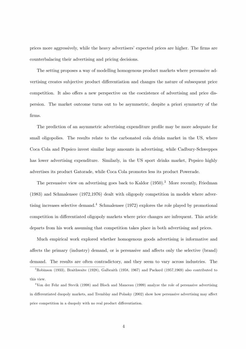
Proposition 2 The following distribution functions represent a mixed strategy Nash equilibrium

of the pricing subgame (Ai, πi; i ∈ N).

Fn (p) =

0 for p < L = (r − c)Un−1

I + Un−1+ c

(I + Un−1)I

− (r − c)Un−1I (p− c)

for L ≤ p ≤ r

1 for p ≥ r

,

Fn−1 (p) =

0 for p < L = (r − c)Un−1

I + Un−1+ c

(I + Un)

I− (r − c)Un−1 (I + Un)

I (p− c) (I + Un−1)for L ≤ p ≤ r

1 for p ≥ r

,

Fk (p) =

0 for p < r

1 for p ≥ r

for ∀k = 1, 2...n− 2.

16

r

1

0

F

p)

[

)

L

Un+I/ Un-1+I

Fn(p) Fn-1(p) Fk(p), k=1,...n-2

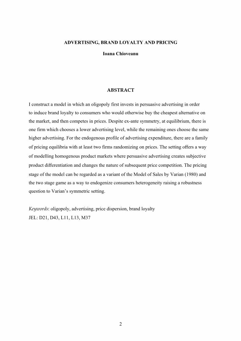
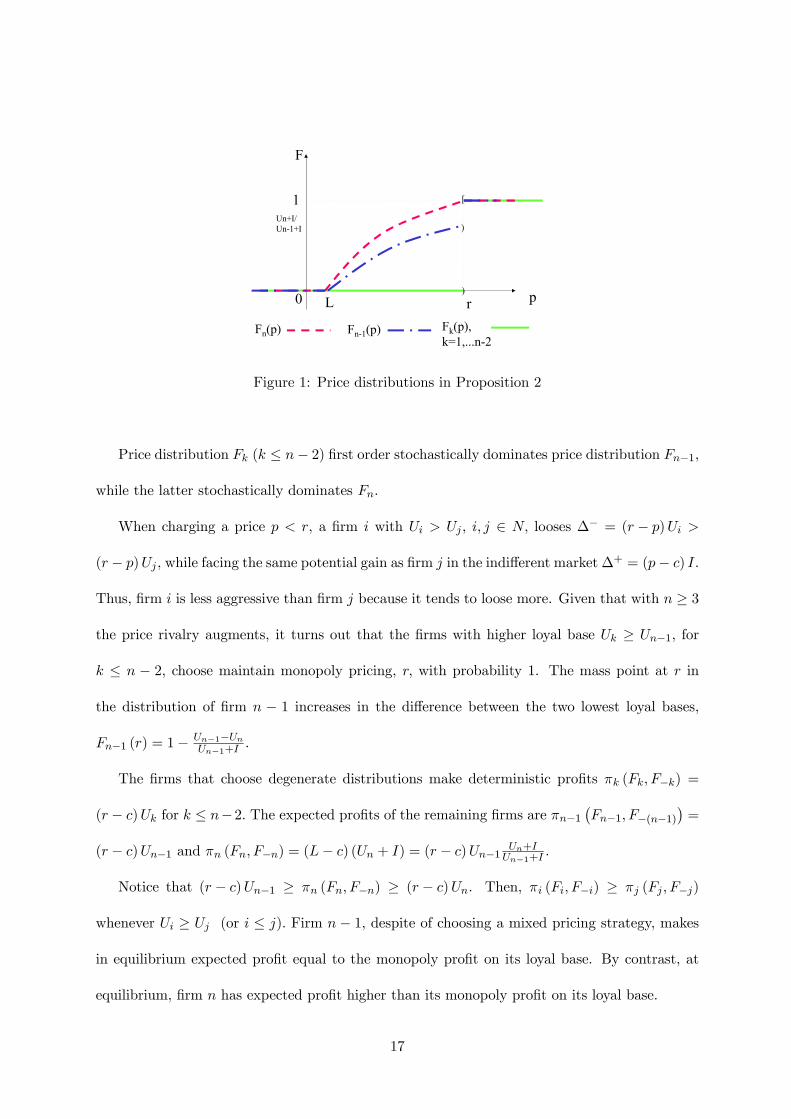
Figure 1: Price distributions in Proposition 2

Price distribution Fk (k ≤ n− 2) first order stochastically dominates price distribution Fn−1,

while the latter stochastically dominates Fn.

When charging a price p < r, a firm i with Ui > Uj , i, j ∈ N, looses ∆− = (r − p)Ui >

(r − p)Uj , while facing the same potential gain as firm j in the indifferent market∆+ = (p− c) I.

Thus, firm i is less aggressive than firm j because it tends to loose more. Given that with n ≥ 3

the price rivalry augments, it turns out that the firms with higher loyal base Uk ≥ Un−1, for

k ≤ n − 2, choose maintain monopoly pricing, r, with probability 1. The mass point at r in

the distribution of firm n − 1 increases in the difference between the two lowest loyal bases,

Fn−1 (r) = 1− Un−1−UnUn−1+I .

The firms that choose degenerate distributions make deterministic profits πk (Fk, F−k) =

(r − c)Uk for k ≤ n−2. The expected profits of the remaining firms are πn−1¡Fn−1, F−(n−1)

¢=

(r − c)Un−1 and πn (Fn, F−n) = (L− c) (Un + I) = (r − c)Un−1 Un+IUn−1+I .

Notice that (r − c)Un−1 ≥ πn (Fn, F−n) ≥ (r − c)Un. Then, πi (Fi, F−i) ≥ πj (Fj , F−j)

whenever Ui ≥ Uj (or i ≤ j). Firm n− 1, despite of choosing a mixed pricing strategy, makes

in equilibrium expected profit equal to the monopoly profit on its loyal base. By contrast, at

equilibrium, firm n has expected profit higher than its monopoly profit on its loyal base.

17

The equilibrium in Proposition 2 predicts price dispersion in relatively small markets. When

the number of firms increases, so does the number of firms that permanently choose monopoly

pricing, and the dispersion in prices tends to become insignificant. The higher the number of

competitors the lower the chances of an individual firm to win the indifferent market. When the

number of competitors is higher more firms prefer to rely on their locked-in markets and act as

monopolists rather than engage in aggressive pricing.

Narasimhan (1988) offers an explanation for price dispersion in competitive markets based

on consumer loyalty. He restricts attention to a duopoly. The present paper offers an extension

of his setting to oligopoly. With arbitrary weakly ordered profiles of loyal groups, only the two

lowest loyal base firms engage in price promotions20 and, for this reason, the potential of this

model to explain market wide price promotions is limited when the number of firms increases.

The next Proposition presents a special uniqueness result.

Proposition 3 If firms employ convex supports, the equilibrium stated in Proposition 2 is the

unique equilibrium that applies to any weakly ordered profile of loyal bases.

However, when n > 2, for particular profiles of loyal groups, there are other pricing equilibria,

as well. In all equilibria the firms make the same expected payoffs. This allows to solve the

reduced form game in the first stage. I present another equilibrium valid for the specific profile

Un < Un−1 = ... = U1, which turns out to be relevant for the present analysis. The proof is

similar to that of proposition 2.

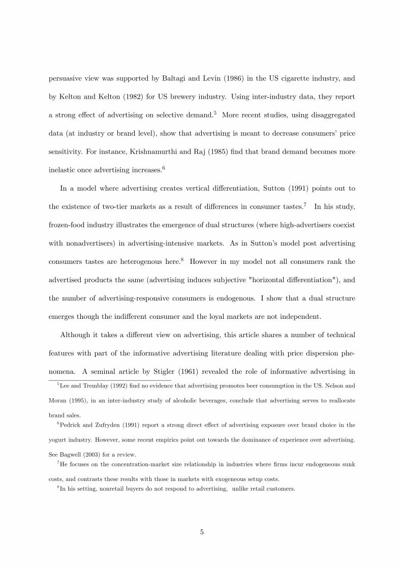
Proposition 4 If the loyal bases satisfy Ui = U for i ≤ n−1 and Un < U , there exists a pricing

equilibrium with all firms randomizing over the same convex support. The firms choose prices

20Pricing below the monopoly level with positive probability is interpreted as a price promotion.

18

according to the following distributions:

Fi (p) =

0 for p < L = (r − c)U

I + U+ c

1−·(L− c) (I + Un)

I (p− c)− Un

I

¸ 1n−1

for L ≤ p < r

1 for p ≥ r

for i = 1, 2...n− 1,

Fn (p) =

0 for p < L = (r − c)U

I + U+ c

1−·(r − p)U

I (p− c)

¸ ·L (I + Un)

I (p− c)− Un

I

¸2−nn−1

for L ≤ p ≤ r

1 for p ≥ r

.

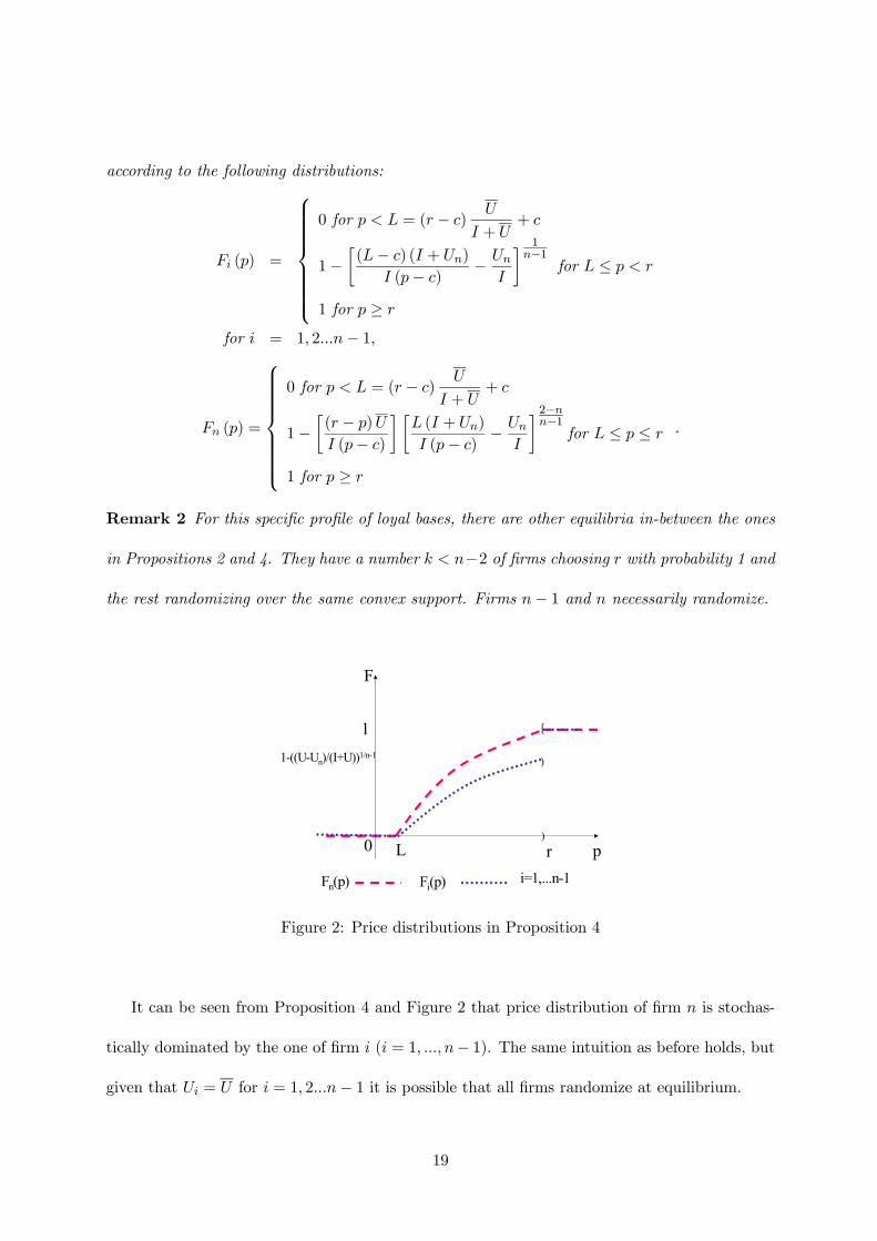
Remark 2 For this specific profile of loyal bases, there are other equilibria in-between the ones

in Propositions 2 and 4. They have a number k < n−2 of firms choosing r with probability 1 and

the rest randomizing over the same convex support. Firms n− 1 and n necessarily randomize.

r

1

0

F

p)

[

)

L

Fn(p) Fi(p) i=1,...n-1

1-((U-Un)/(I+U))1/n-1

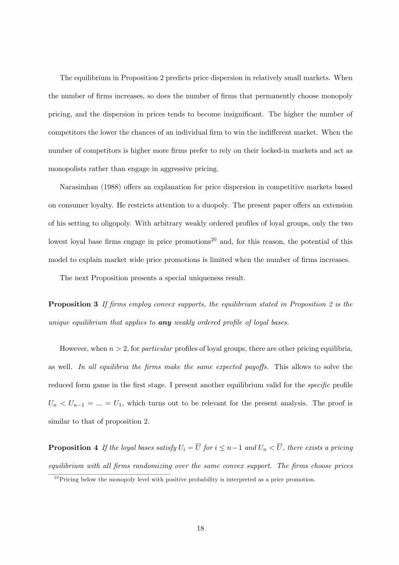
Figure 2: Price distributions in Proposition 4

It can be seen from Proposition 4 and Figure 2 that price distribution of firm n is stochas-

tically dominated by the one of firm i (i = 1, ..., n− 1). The same intuition as before holds, but

given that Ui = U for i = 1, 2...n− 1 it is possible that all firms randomize at equilibrium.

19

The pricing subgame maybe understood as a variant of Varian’s “Model of Sales”, with

asymmetric captured consumer bases. “A Model of Sales” is meant to describe markets which

exhibit price dispersion, despite the existence of at least some rational consumers.21 The model

interprets sales as a way to discriminate between consumers who are assumed to come in two

types, informed and uninformed. All consumers have a common reservation value and they

purchase a unit of the good whenever the price does not exceed the valuation, the uninformed

ones choose randomly a shop and the informed ones buy from the cheapest seller. The paper by

Varian restricts attention to the symmetric equilibrium of the symmetric game (with uninformed

consumers evenly split amongst the firms).22 However, there exists a family of asymmetric

equilibria of the symmetric game.23

The present setting offers a way of endogenizing the creation of locked-in consumers, and it

raises a robustness question to Varian’s symmetric setting because it turns out that at equilib-

rium the captured bases are asymmetric.

Extending Varian’s model, Baye, Kovenock and de Vries (1992) construct a metagame in

which consumers are also players. In the first stage, uninformed consumers and firms move

simultaneously. Firms choose a price distribution and the uninformed consumers decide from

which firms to purchase. In the second stage, the informed consumers choose the seller they will

buy from. Given that the asymmetric price distributions can be ranked by first-order stochastic

dominance, they show that the unique subgame perfect equilibrium of the extensive game is the

symmetric one. However, this follows from the equilibrium consistency requirement that a firm

21Varian is concerned with understanding “temporal price dispersion” rather than “spatial price dispersion”.

That is, intertemporal changes in the pricing of a given firm rather than cross-sectional price volatility.22 If the optimal pricing distributions are continuous and the supports are convex, then the equilibrium is

symmetric (Proposition 9 of Varian (1980), p.658). See the Appendix for a transcription of this Proposition.23A comprehensive analysis of all the asymmetric equilibria of the symmetric game is provided by Baye,

Kovenock and deVries (1992).

20

with higher expected price cannot have a larger uninformed consumer base.

4 Advertising Expenditure Choices

In this section, I derive the equilibrium of the reduced form game in the first stage where

oligopolists simultaneously choose an advertising expenditure. Their payoffs are the profits

emerging in the pricing stage less the chosen advertising expenditure. The gross of advertising

cost profits with loyal bases Un ≤ Un−1 ≤ ... ≤ U1 are:

Eπj = (r − c)Uj , ∀j ∈ N \ {n} ;

Eπn = (L− c) (Un + I) = (r − c)Vn

where Vn = Un−1(Un + I)

(Un−1 + I).24

The loyal consumer group of firm i (Ui) is given by

Ui (αi, α−i) = Si (αi, α−i)U (Σjαj) .

Each firm may invest in generating loyal consumers and the total number of brand loyals on

the market is determined by the aggregate expenditure. The advertising technology is imperfect

and there is always a fraction of consumers who are not persuaded (or reached) by advertising.

This fraction forms the brand indifferent group (I) which buys the cheapest product,

I = 1−nXi=1

Ui (αi, α−i) = 1− U (Σiαi) .

Under the assumptions made so far, the loyal group of a firm is increasing in own advertising. The

incremental consumers may proceed from the brand indifferent group (U 0 (Σiαi) > 0) or from

rival’s loyal groups³∂Si(αi,α−i)

∂αi≥ 0

´. The last source leaves open the possibility of reciprocal

cancellation across brands.25 An increase in rival advertising has two conflictive effects on the24Note that if Un = Un−1, Vn = Un.25Metwally (1975,1976) and Lambin (1976) find empirical evidence in this sense.

21

loyal base of a firm. There is a positive effect due to the increase in the total number of loyals

(U 0 (Σiαi) > 0) and a negative one due to a decrease in the share of the firm³∂Si(αi,α−i)

∂αj≤ 0

´.

I assume that the overall effect of rival advertising is negative.

A1: ∂2Ui∂α2i

< 0, ∂2Ui∂α2i≤ ∂2Ui

∂αi∂αjfor i, j < n and ∂2Vn

∂α2n< 0; ∂Ui

∂αi(0, α−i) > 1

r−c and∂Vn∂αn

(0, α−n) >

1r−c .

A2: ∂2Ui∂αi∂αj

≤ 0, ∂2Vn∂αn∂αj

≤ 0.

Assumptions A1 and A2 guarantee the existence of equilibrium.

With αn ≤ αn−1 ≤ ... ≤ α1, firm j 6= n maximizes net of advertising expenditure profit:

πj = (r − c)SjU (Σiαi)− αj = πH .

Firm n maximizes its expected profit net of advertising costs:

πn = (r − c)Sn−1U (Σiαi)(SnU (Σiαi) + I)

(Sn−1U (Σiαi) + I)− αn = πL.

Notice that πH = πL when αn = αn−1. The FOC of the maximization problems above implicitly

define α∗n (α−n) and α∗j (α−j) for j ∈ N \ {n} .

For a symmetric equilibrium α∗ to exist, firm n should not have incentives to decrease, and

the other firms should not have incentives to increase, when choosing α∗.

∂πn∂αn

¡α∗, α∗−n

¢ ≥ 0 and ∂πj∂αj

¡α∗, α∗−j

¢ ≤ 0 for all j ∈ N \ {n} .

In Appendix B it is shown that this requirement leads to a contradiction. Together with the

optimization problem above, this proves the following result.

Proposition 5 Under A1, in any pure strategy Nash equilibrium of the reduced form advertising

game, αn < αi = αj for ∀i, j ∈ NÂ {n} . The values of αn and αi (∀i ∈ NÂ {n}) are implicitly

defined by the FOCs.

22

The following example illustrates that a symmetric advertising profile cannot form part of

an equilibrium.26

Example 1 Let Si (αi, α−i) = αiΣjαj

for ∀i ∈ N, U (Σjαj) =Σjαj1+Σjαj

, n = 2 and c = 0.27 Then at

α1 = α2 = α, the symmetric payoffs are given by πS1 = πS2 = r α1+2α−α. For r <

¡1+2αα

¢2(1 + α) ,

firm 1 has incentives to deviate to αL1 = αq

r1+α − (1 + α) < α. For r ≥ ¡1+2αα

¢2(1 + α) , firm

1 has incentives to deviate to αH1 =pr (1 + α)− (1 + α) > α.28

A1 requires that ∂2Ui∂α2i≤ ∂2Ui

∂αi∂αj. This guarantees that given αn, firms i, j ∈ NÂ {n} choose

αi = αj at equilibrium and allows to fully define the equilibrium outcome. Without this restric-

tion more general asymmetries may arise at equilibrium. However, αn < αi for ∀i ∈ NÂ {n} in

any reduced form game equilibrium.

Proposition 6 Under A1 and A2, the advertising expenditure in Proposition 5, together with

any of the pricing strategy profiles in Proposition 2, Proposition 4, or Remark 2 give the subgame

perfect equilibria of the two stage game.

To see the role played by submodularity, consider a duopoly. Let (α1, α2) with α1 > α2

be a candidate equilibrium. As ∂πH∂αH

(α1, α2) = 0, if firm 2 deviates to α ≥ α1 its profits are

lower. For ∀α ≥ α1, its marginal profit is∂πH∂αH

(α, α1) < ∂πH∂αH

(α1, α1) ≤ ∂πH∂αH

(α1, α2) = 0.

The first inequality follows from strict concavity and the second from submodularity. Then

πH (α,α1) < πH (α1, α1) = πL (α1, α1) ≤ πL (α2, α1) . A symmetric of this argument can be26 I use this example for computational convenience. Though well defined, it satisfies A1, but not A2. An

example satisfying both A1 and A2 for n = 2 is Si (αi, α−i) =α1/6i

Σiα1/6i

for ∀i ∈ N, U (Σiαi) =Σiα

1/6i

1+Σiα1/6i

.

27The sharing rule in the example, Si (αi, α−i) = αiΣjαj

maybe interpreted as a probability that an arbitrary

loyal consumer chooses firm i. This probability is nonincreasing in i and thus a firm with higher advertising is

more likely to be chosen by a loyal consumer.

28π1¡αL1 , α

¢ − πS1 (α,α) = (1 + 2α)−1hαq

r1+α

− (1 + 2α)i2

> 0 and π1¡αH1 , α

¢ − πS1 (α,α) =

(1 + 2α)−1hαpr (1 + α)− (1 + 2α)

i2> 0.

23

used to show that firm 1 does not have incentives to deviate to α ≤ α2. A general proof for

arbitrary number of firms is provided in the appendix. However A2 is sufficient but not necessary

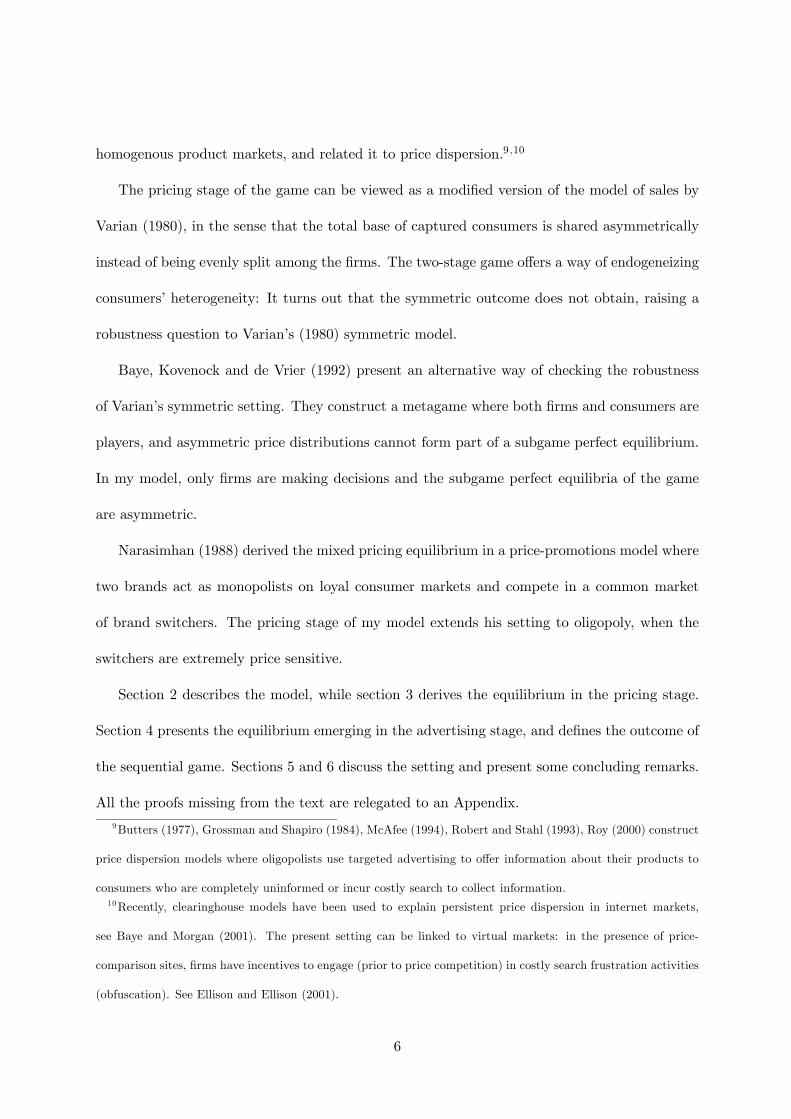
for an asymmetric equilibrium to exist. This can be easily seen in Example 1. For r−c = 16, the

candidate equilibrium is (α1, α2) = (3.94, 2.15). Firm 1 does not have incentives to leapfrog firm

2: Its profits on [0, 2.15] are maximized at 1.7, and π1 (1.7, 2.15) = 4.38 < π1 (3.94, 2.15) = 4.95.

Firm 2 does not have incentives to leapfrog firm 1: Its profits on [3.94,∞) are maximized at

3.95, and π2 (3.95, 3.94) = 3.15 < π2 (2.15, 3.94) = 3.52. The best response graph is presented in

Appendix B.

Other models that yield such asymmetric equilibria can be found in McAffee (1993) and Amir

and Wooders (2000). In these models (as in the present one) payoff functions are submodular

and best response functions jump down over the diagonal.

The asymmetric equilibrium follows from the fact that firms weigh their first and second

stage decisions. A larger first stage investment triggers less aggressive second stage pricing,

while a lower investment supposes a more aggressive pricing strategy.

Although they are identical, at equilibrium, firms choose asymmetric advertising expenditure.

This asymmetry follows from the choice of mixed pricing strategies. There is one firm with a

strictly lower advertising level (firm n in the example) and with the lowest loyal group. All other

firms choose the same higher level of advertising and have equal larger loyal consumer bases.

Although in Example 1 the low advertiser makes lower net of advertising cost profits than its

rival, this may not be true in general.

The lowest loyal group firm prices more aggressively, has higher probability of being the

winner of the indifferent market, and makes lower gross expected profits. All other firms price

less aggressive and make equal gross of advertising expenditure profits equal to monopoly profit

on their loyal market.

24

4.1 A Random Utility Interpretation

In this subsection I offer a possible microfoundation to the demand system considered in the

case of a duopoly. A random utility model can lead to the proportional market sharing function

Si =αi

Σjαjused in the examples, when consumers respond to advertising and prices, but are

short-sighted. With a duopoly there is a unique mixed pricing equilibrium where both firms

randomize, and E (pi | pi < r) = E (pj | pj < r) . In the marketing literature, price dispersion

models are used to explain price promotions. The expected price conditional on a brand being

being priced lower than r is thought of as the average discounted price, while 1−F (r) measures

the frequency of discounts. Considering that loyal consumers are myopic and care only about

the average discount and advertising, the proportional market sharing function, Si = αiΣjαj

, can

be derived from a random utility model.29

5 Discussion

While there is no doubt that advertising plays an important informative role in the economy, not

less numerous are the occasions in which it does not provide any relevant information on price

or product characteristics. In many homogenous product markets, advertising only operates

a redistribution of the consumers among the sellers. Many advertising campaigns and a great

deal of the TV spot advertising have rather an emotional content and try to attract consumers

associating the product with attitudes or feelings that have no relevant relation to the product

or its consumption.30

29Consumers have idiosyncratic preferences over the brands and each consumer chooses the one that has the

greatest brand advertising-average discount differential (see Anderson, De Palma and Thisse (1992)).30Explaining the content of Chevrolet TV ads for automobiles “Heartbeat of America”, broadcasted in 1988,

General Motors advertising executive Sean Fitzpatrick observed that they “may look disorganized, but every

detail is cold-heartedly calculated. People see the scenes they want to identify with.[...] It’s not verbal. It’s

25

Loewenstein (2001) remarks “[w]hile conventional models of decision making can make sense

of advertisements that provide information about products (whether informative or misleading),

much advertising- for example, depicting happy, attractive friends drinking Coca-Cola seem to

have little informational content. Instead such advertising seems to be intended to create mental

associations that operate in both directions, causing one to think that one should be drinking

Coca-Cola if one is with friend (by evoking a choice heuristic) and to infer one that one must

be having fun if one is drinking Coca-Cola (playing on the difficulty of evaluating one’s hedonic

state).”31 He points out to the importance of situational construals, people “often seem to behave

according to a two-stage process in which they first attempt to figure out what kind of situation

they are in and then adopt choice rules that seem appropriate for that situation”. Persuasive

advertising could be a way to influence such categorization through mental associations. As

an example of association, Pepsi’s 1997 GeneratioNext campaign defines itself as being “about

everything that is young and fresh, a celebration of the creative spirit. It is about the kind of

attitude that challenges the norm with new ideas, at every step of the way”.32 Similarly, Perrier

significantly strengthened its position in the French mineral water market with its advertising

campaign directed to the younger generation, under the slogan “Perrier c’est fou” (“Perrier is

not rational. It’s emotional, just the way people buy cars.” (see Scherer and Ross 1990 p.573, originally from

“On the Road again, with a Passion”, New York Times October 10th, 1988) Also, commenting on the new

trends in television advertising, James Twitchell Professor of advertising at the University of Florida noted that

“Advertising is becoming art. You don’t need it, but it’s fun to look at” (see Herald Tribune, January 10th, 2003

p.7).31 In the same spirit Camerer, Loewenstein and Prelec (forthcoming) notice "Prevailing models of advertising

assume that ads convey information or signal a product’s quality or, for "network" or "status" goods, a product’s

likely popularity. Many of these models seem like strained attempts to explain effects of advertising without

incorporating the obvious intuition that advertising taps the neural circuitry of reward and desire".32See www.pepsi.com. Coke relies on more traditional values in its “Coca Cola...Real” campaign. See also

Tremblay and Polasky (2002).

26

crazy”) making the product be perceived as very fashioned.33 These considerations support the

persuasive view on advertising and offer a justification for the stylized setting here.

The present analysis suggests that high advertisers tend to have higher prices. Often, blind

tests show that consumers perceive highly advertised brands as different.34 The model also

predicts the existence of a group of heavy advertisers and of a low advertiser. This is compliant

with the empirical evidence that markets with significant advertising have a two-tier structure.

The endogenous asymmetric advertising profile is more suitable for small oligopolies. In the

US sport drinks market, Coca Cola and Pepsico are the two major suppliers. In 2002, Pepsico

invested 125 millions to promote its product Gatorade, while Coca Cola invested 11 millions to

advertise its product Powerade.

Several extensions to this work are worth mentioning. A major limitation of the present

model is the extreme post-advertising heterogeneity of consumers: Loyal consumers are ex-

tremely advertising responsive, while the indifferent ones continue to be extremely price sensi-

tive. One may consider a smoother distribution of advertising-induced switching costs. Moreover

indifferent consumers are aware about existence of all products. Possibly it is more realistic to

assume that the indifferent consumers know only the prices of some sellers.

6 Conclusions

The present article proposes a way to model the effects of persuasive advertising on price compe-

tition in a homogenous product market. I solve a two stage game in which an oligopoly competes,

33See J. Sutton (1991), p.253. Even more relevant for the present discussion is the subsequent campaign of

Perrier under the (only literary) meaningless slogan “Ferrier c’est pou”, a partial toggle of its initial slogan.34“Double-blind experiments have repeatedly demonstrated that consumers cannot consistently distinguish

premium from popular-priced beer brands, but exhibit definite preferences for the premium brands when labels

are affixed-correctly or not.” (see Scherer and Ross 1990 p.582)

27

first, in persuasive advertising and, then, in prices. Advertising results in the creation of a loyal

group attached to the firm. The equilibrium outcome exhibits price dispersion, although it is

possible to have in equilibrium up to n − 2 firms choosing monopoly pricing with probability

1. The endogenous advertising choices of the firms reflect the asymmetry in the mixed pricing

strategies and, at equilibrium, there is one firm that chooses a lower level of advertising and the

remaining ones choose the same higher advertising. The model predicts an asymmetric mar-

ket outcome despite initial symmetry of firms, and suggests how persuasive advertising may be

successfully used to relax price competition.

7 Appendix

7.1 Appendix A

Proof of Proposition 1. Assume¡p∗i , p

∗−i¢is a pure strategy Nash equilibrium profile. Then,

by the definition of such equilibrium, @pi such that πi¡pi, p

∗−i¢> πi

¡p∗i , p

∗−i¢. Let i be such that

p∗i ≤ p∗k,∀k 6= i. Consider first the case where p∗i = p∗j 6= c, where p∗j = {min p∗k | k ∈ N \ {i}} .

Then πi¡p∗i , p

∗−i¢= (p∗i − c) (Ui + Iφ) < πi

¡p∗i − ε, p∗−i

¢= (p∗i − c− ε) (Ui + I) . Hence, ∃pi =

p∗i −ε, for 0 < ε <(p∗i−c)(1−φ)I

Ui+I, such that πi

¡pi, p

∗−i¢> πi

¡p∗i , p

∗−i¢. This argument fails at p∗i =

p∗j = c, but πi¡c, p∗−i

¢= 0 < πi

¡r, p∗−i

¢. Consider, finally, the case p∗i < p∗j , where p

∗j ={min p

∗k |

k ∈ N \ {i}}. Then πi¡p∗i , p

∗−i¢= (p∗i − c) (Ui + I) < πi

¡p∗i + ε, p∗−i

¢= (p∗i − c+ ε) (Ui + I)

whenever ε < p∗j−p∗i . Then, ∃pi = p∗i+ε, for 0 < ε < p∗j−p∗i , such that πi¡pi, p

∗−i¢> πi

¡p∗i , p

∗−i¢.

The cases presented above complete the proof of nonexistence of a pure strategy Bertrand-Nash

equilibrium in the game (Ai, πi; i ∈ N) .

Proof of Lemma 4. I prove that Fi (p) is continuous on [Li, r) by contradiction. Assume

PFi (p) > 0 for some p < r. For simplicity, let c = 0.

Case 1. Suppose ∃ j such that Fj (p+ ε)− Fj (p) > 0. Then, the variation in the profit of firm

28

j when pricing at p− ε instead of p+ ε is:

(p− ε)£Uj + Iϕj (p− ε)

¤− (p+ ε)£Uj + Iϕj (p+ ε)

¤ ≥(p− ε)

£Uj + Iϕj (p− ε)

¤− (p+ ε)£Uj + Iϕj (p− ε)

¤=

− 2εUj + IPn−1

k=011+k

PM⊆N−j|M |=k

[Qn

m=1m∈M

PFm (p− ε)Qn

l=1l/∈Ml 6=i

(1− Fl (p− ε))]

[(p− ε) (1− Fi (p− ε))− (p+ ε) (1− Fi (p+ ε))]

=

− 2εUj + IPn−1

k=011+k

PM⊆N−j|M |=k

[Qn

m=1m∈M

PFm (p− ε)Qn

l=1l/∈Ml 6=i

(1− Fl (p− ε))]

[(p+ ε) (Fi (p+ ε)− Fi (p− ε))− 2ε]

.

Let eF εj be the sequence of unilateral deviations defined by eFj (p0) = Fj (p

0) for p0 < p − ε

and P eFj (p− ε) = Fj (p+ ε) − Fj (p) for p0 > p + ε. Since limε→0πj (Fj , F−j) − πj

³ eFj , F−j´ =pIkϕj (p)PFi (p) > 0 firm j has incentives for unilateral deviation.

Case 2. Suppose @j such that Fj (p+ ε)− Fj (p) > 0, then

πi (p+ ε) = (p+ ε) (Ui + Iϕi (p+ ε)) > p (Ui + Iϕi (p)) = πi (p).

Then firm i has incentives to deviate.

It follows that for p < r, PFi (p) = 0 for all i. (QED)

Proof of Proposition 3. Suppose there exists a Nash equilibrium in prices different than

the one in Proposition 2. Let bS∗i be the associated supports of the price distributions. Forsimplicity, let c = 0.

By Lemma 2, {r} ⊆ bS∗i for all i. Let K =ni | {r} 6= bS∗i o .

By Proposition 1 and Lemma 1, |K| ≥ 2.

a) Assume, first, |K| > 2.

By Lemma 3, ∃l ∈ N, such that f∗l (r) = 0. Notice that for all i ∈ NÂK, f∗i (r) = 1. Hence,

l ∈ K.

By Lemma 1, ∃i, k ∈ N , s.t. Li = min bS∗i = Lk = min bS∗ka1) Suppose that l = i. Let k, h ∈ K, k 6= l 6= h and Ll = Lk.

29

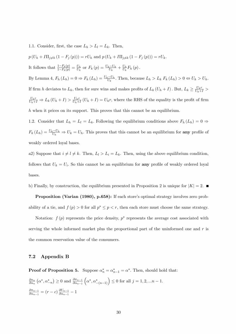
1.1. Consider, first, the case Lh > Ll = Lk. Then,

p (Uh + IΠj 6=h (1− Fj (p))) = rUh and p (Uk + IΠj 6=k (1− Fj (p))) = rUk.

It follows that 1−Fk(p)1−Fh(p) =UhUkor Fk (p) =

Uk−UhUk

+ UhUkFh (p) .

By Lemma 4, Fh (Lh) = 0⇒ Fk (Lh) =Uk−UhUk

. Then, because Lh > Lk Fk (Lh) > 0⇔ Uk > Uh.

If firm h deviates to Lk, then for sure wins and makes profits of Lk (Uh + I) . But, Lk ≥ UkrUk+I

>

UhrUh+I

⇒ Lk (Uh + I) > UhrUh+I

(Uh + I) = Uhr, where the RHS of the equality is the profit of firm

h when it prices on its support. This proves that this cannot be an equilibrium.

1.2. Consider that Lh = Ll = Lk. Following the equilibrium conditions above Fh (Lh) = 0 ⇒

Fk (Lh) =Uk−UhUk

⇒ Uk = Uh. This proves that this cannot be an equilibrium for any profile of

weakly ordered loyal bases.

a2) Suppose that i 6= l 6= k. Then, Ll > Li = Lk. Then, using the above equilibrium condition,

follows that Uk = Ui. So this cannot be an equilibrium for any profile of weakly ordered loyal

bases.

b) Finally, by construction, the equilibrium presented in Proposition 2 is unique for |K| = 2.

Proposition (Varian (1980), p.658): If each store’s optimal strategy involves zero prob-

ability of a tie, and f (p) > 0 for all p∗ ≤ p < r, then each store must choose the same strategy.

Notation: f (p) represents the price density, p∗ represents the average cost associated with

serving the whole informed market plus the proportional part of the uninformed one and r is

the common reservation value of the consumers.

7.2 Appendix B

Proof of Proposition 5. Suppose α∗n = α∗n−1 = α∗. Then, should hold that:

∂πn∂αn

¡α∗, α∗−n

¢ ≥ 0 and ∂πn−1∂αn−1

³α∗, α∗−(n−1)

´≤ 0 for all j = 1, 2, ...n− 1.

∂πn−1∂αn−1 = (r − c) ∂Un−1∂αn−1 − 1

30

∂πn∂αn

= (r − c) (Un−1 + I)−2

∂Un−1∂αn

(Un + I) (Un−1 + I)+

Un−1h³

∂Un∂αn− U

0´(Un−1 + I)−

³∂Un−1∂αn

− U0´(Un + I)

i− 1

The above inequalities imply the following one:

∂Un−1∂αn−1 ≤

∂Un−1∂αn

(Un + I) (Un−1 + I)−1+

Un−1h³

∂Un∂αn− U 0

´(Un−1 + I)−

³∂Un−1∂αn

− U 0´(Un + I)

i(Un−1 + I)−2

Notice that Sn¡α∗, α∗−n

¢= Sn−1

³α∗, α∗−(n−1)

´and ∂Sn

∂αn

¡α∗, α∗−n

¢= ∂Sn−1

∂αn−1

³α∗, α∗−(n−1)

´. In

effect, Un

¡α∗, α∗−n

¢= Un−1

³α∗, α∗−(n−1)

´and ∂Un

∂αn

¡α∗, α∗−n

¢= ∂Un−1

∂αn−1

³α∗, α∗−(n−1)

´for α∗n =

α∗n−1 = α∗, given that Un−1 = Sn−1U and ∂Un−1∂αn−1 =

∂Sn−1∂αn−1U + Sn−1U 0. Then, the last inequality

becomes: ∂Un−1∂αn−1 ≤

∂Un−1∂αn

+Un−1

h∂Un∂αn

−∂Un−1∂αn

i(Un−1+I) ⇔

∂Sn−1∂αn−1U + Sn−1U 0 ≤ ∂Sn−1

∂αnU + Sn−1U 0 + Sn−1U

∂Sn∂αn

U+SnU 0−∂Sn−1∂αn

U−Sn−1U 0Sn−1U+1−U ⇔

∂Sn−1∂αn−1U ≤

∂Sn−1∂αn

U + Sn−1U∂Sn∂αn

U−∂Sn−1∂αn

U

Sn−1U+1−U ⇔³∂Sn−1∂αn−1 −

∂Sn−1∂αn

´U (1− U) ≤ 0⇔

Since ∂Sn−1∂αn−1 > 0 and

∂Sn−1∂αn

< 0, the inequality holds only if U = 0 or U = 1. But,

U = 1 ⇒ Σiαi → ∞ and U > 0 as ∂Un−1∂αn−1

¡0, α−(n−1)

¢> 0. A contradiction. Then, αn < αn−1

at equilibrium.

Consider i < j < n, the FOC imply ∂Ui∂αi− 1

r−c = 0 and ∂Uj∂αj− 1

r−c = 0. By A1 αi > αj

implies ∂Ui∂αi

<∂Uj∂αj

. Since αi ≥ αj , it follows that αi = αj for i, j 6= n. This establishes that

αn < αn−1 = ... = α1.

Proof of Proposition 6. To make sure that the candidate maximum defines the first

stage strategies in a subgame perfect equilibrium, firm j = 1, ...n− 1 should not have incentives

to leapfrog firm n, and firm n should not have incentives to leapfrog its rivals.

Let α∗i be the equilibrium choice of firm i ∈ NÂ {n} , α∗n be the equilibrium choice of firm n and

α∗ ∈ Rn−2 be the vector of equilibrium choices if firms j ∈ NÂ {i, n} . πi,1 is the own partial

derivative of firm i’s profit function.

31

Consider firm n. Its profits are:

πn (α, α∗i , α

∗) =

(r − c)Vn (α,α

∗i , α

∗)− α = πLn (α,α∗i , α

∗) if α ≤ α∗i

(r − c)Un (α, α∗i , α

∗)− α = πHn (α, α∗i , α

∗) if α > α∗i

,

where α is the choice of firm n.

Consider the case α > α∗i , then the following is true:

0 = πHn,1 (α∗i , α

∗n, α

∗) > πHn,1 (α, α∗n, α

∗) ≥ πHn,1 (α, α∗i , α

∗) . The first inequality follows from strict

concavity (A1) and the second from submodularity of Un (A2). Then, firm n has incentives to

decrease.

When α ≤ α∗i , the profit function is concave and, hence, maximized at α = α∗n.

Consider firm j ∈ NÂ {n}. Its profits are:

πj (α, α∗n, α

∗) =

(r − c)Uj (α, α

∗n, α

∗)− α = πHj (α,α∗n, α

∗) if α ≥ α∗n

(r − c)Vj (α, α∗n, α

∗)− α = πLj (α, α∗n, α

∗) if α < α∗n

,

where Vj (α, α∗n, α∗) = Un (α∗n, α, α

∗) Uj(α,α∗n,α

∗)+IUn(α∗n,α,α∗)+I

and α is the choice of firm j.

Consider α < α∗n, then the following is true:

0 = πLj,1 (α∗n, α

∗i , α

∗) < πLj,1 (α, α∗i , α

∗) ≤ πLj,1 (α,α∗n, α

∗) .

The first inequality follows from strict concavity (A1) and the second from submodularity of

Vj (A2). Then, firm j has incentives to increase. When α ≥ α∗n, the profit function is strictly

concave and, hence, maximized at α = α∗j .

Example 1 Best response functions for r − c = 16.

Given rival’s choice α, firm i’s best response would be αHi (α) = 4 (1 + α)12 − (1 + α) if it

chose αi ≥ α and would be αLi (α) = 4α (1 + α)−12 − (1 + α) if it chose αi < α.

The corresponding profits are:

πi (α) =

πHi (α) = 16− 8 (1 + α)

12 + (1 + α) for αi ≥ α

πLi (α) = 16α (1 + α)−1 − 8α (1 + α)−12 + (1 + α) for αi < α

.

32

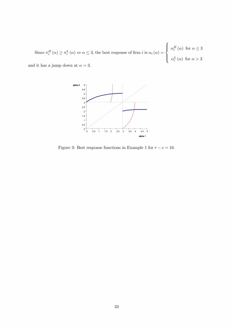
Since πHi (α) ≥ πLi (α)⇔ α ≤ 3, the best response of firm i is αi (α) =

αHi (α) for α ≤ 3

αLi (α) for α > 3

and it has a jump down at α = 3.

54.543.532.521.510.50

5

4.5

4

3.5

3

2.5

2

1.5

1

0.5

0

alpha 1

alpha 2

alpha 1

alpha 2

Figure 3: Best response functions in Example 1 for r − c = 16.

33

8 References

Advertising Age, June 28th, 2004. 100 Leading National Advertisers.

Anderson, S., De Palma, A., Thisse, J.-F., 1992. Discrete Choice Theory of Product Differ-

entiation. MIT Press.

Bagwell, K., 2002. The Economic Analysis of Advertising. Columbia University.

Baye, M., Kovenock, D., de Vries, C., 1992. It Takes Two to Tango: Equilibria in a Model

of Sales. Games and Economic Behavior 4, p.493.

Baye,M., Morgan, J., 2001. Information Gatekeepers on the Internet and the Competitive-

ness of Homogeneous Product Markets. American Economic Review 91, p.454

Brown, R.S., 1978. Estimating Advantages to Large Scale Advertising. Review of Economic

Studies 60, p.428.

Butters, G., 1977. Equilibrium Distributions of Sales and Advertising Prices. Review of

Economic Studies 44.3, p.465.

Camerer C., Loewenstein G., Prelec D., (forthcoming) Neuroeconomics: How Neuroscience

Can Inform Economics. Journal of Economic Literature

Dasgupta, P., Maskin, E., 1986. The Existence of Equilibrium in Discontinuous Economic

Games, I: Theory. Review of Economic Studies 53, p.1.

Friedman, J., 1983. Oligopoly Theory. Cambridge University Press.

Herald Tribune, January 10th, 2003. As viewers zap ads, TV hatches an old plan p.1/7.

Kahneman D., 2003. Maps of Bounded Rationality: Psychology for Behavioral Economics.

American Economic Review 93, p.1449.

Kaldor N.V., 1950. The Economic Aspects of Advertising. Review of Economic Studies 18,

p.1.

Klemperer P., 1987. Markets with Consumer Switching Costs. Quarterly Journal of Eco-

34

nomics 102, p.375.

Kaldor N.V., 1950. The Economic Aspects of Advertising. Review of Economic Studies 18,

p.1.

Krishnamurthi, L., Raj, S.P., 1985. The Effect of Advertising on Consumer Price Sensitivity.

Journal of Marketing Research 22, p.119.

Lambin, J.J., 1976. Advertising, Competition and Market Conduct in Oligopoly Over

Time. North Holland Publishing Co.

Lee, B., Tramblay V., 1992. Advertising and the US Demand for Beer. Applied Economics

24, p.69.

Loewenstein G., 2001. The Creative Destruction of Decision Research. Journal of Consumer

Research 28, p.499.

McAfee, P., 1994. Endogenous Availability, Cartels, and Merger in an Equilibrium Price

Dispersion. Journal of Economic Theory 62, p.24.

Metwally, M.M., 1975. Advertising and Competitive Behavior of Selected Australian Firms.

Review of Economics and Statistics 57, p.417.

Metwally, M.M., 1976. Profitability of Advertising in Australia: A Case Study. Journal of

Industrial Economics 24, p.221.

Narasimhan, C., 1988. Competitive Promotional Strategies. Journal of Business 61, p.427.

Nelson, J., Moran, J., 1995. Advertising and US Alcoholic Beverage Demand: System-wide

Estimates. Applied Economics 27, p.1225.

Pedrick, J., Zufryden, F.,1991. Evaluating the Impact of Advertising Media Plans: A Model

of Consumer Purchase Dynamics Using Single-Source Data. Marketing Science 10.2, p. 111.

Scherer, F.M., Ross, D., 1990. Industrial Market Structure and Economic Performance.

Houghton Mifflin Co. Boston.

35

Schmalensee, R., 1976. The Economics of Advertising. North Holland Publishing Co.

Schmalensee, R., 1976. A Model of Promotional Competition in Oligopoly. Review of

Economic Studies 43, p.493.

Stigler, G.L., 1961. The Economics of Information. Journal of Political Economy 69, p. 213.

Sutton, J., 1991. Sunk Costs and Market Structure, MIT Press.

Tremblay, V., Polasky, S., 2002. Advertising with Subjective Horizontal and Vertical Differ-

entiation. Review of Industrial Organization 20(3), p.253.

Varian, H., 1980. A Model of Sales. American Economic Review 70, p.651.

Vives, X., 1999. Oligopoly Pricing: Old Ideas and New tools. MIT Press.

36