Adverse Selection, Credit, and Efficiency:

the Case of the Missing Market∗†

Alberto Martin‡

December 2010

Abstract

We analyze a standard environment of adverse selection in credit markets. In our envi-

ronment, entrepreneurs who are privately informed about the quality of their projects need

to borrow in order to invest. Conventional wisdom says that, in this class of economies, the

competitive equilibrium is typically inefficient.

We show that this conventional wisdom rests on one implicit assumption: entrepreneurs

can only access monitored lending. If a new set of markets is added to provide entrepreneurs

with additional funds, efficiency can be attained in equilibrium. An important characteristic of

these additional markets is that lending in them must be unmonitored, in the sense that it does

not condition total borrowing or investment by entrepreneurs. This makes it possible to attain

efficiency by pooling all entrepreneurs in the new markets while separating them in the markets

for monitored loans.

Keywords: Adverse Selection, Credit Markets, Collateral, Monitored Lending, Screening

JEL Classification: D82, G20, D62

∗I am grateful to Paolo Siconolfi, Filippo Taddei, Jaume Ventura, Wouter Vergote seminar participants at CREI

and Univesitat Pompeu Fabra, and to participants at the 2008 Annual Meeting of the SED for their comments.

I acknowledge financial support from the Spanish Ministry of Education and Sciences (grants SEJ2005-00126 and

CONSOLIDER-INGENIO 2010 CSD2006-00016, and Juan de la Cierva Program), the Generalitat de Catalunya

(AGAUR, 2005SGR 00490), and from CREA-Barcelona Economics.†An early draft of this paper, circulated in 2006, was titled “On the Efficiency of Financial Markets under Adverse

Selection: the Role of Exclusivity”.‡CREI and Universitat Pompeu Fabra, amartin@crei.cat

1 Introduction

Imagine a setting in which entrepreneurs need to borrow resources to undertake an investment

project. Some entrepreneurs have good projects that succeed often, but others have bad projects

that succeed only seldom. Imagine also that the quality of each investment project is private

information, known to the corresponding entrepreneur but unobservable to outsiders. This is the

typical situation that gives rise to adverse selection in financial markets: if there is a single market

interest rate at which resources can be borrowed, entrepreneurs with bad projects — which are the

ones most likely to fail, and hence to default — will be over-represented in the pool of borrowers.

Of course, borrowing in the real world is subject to lending standards that extend beyond

the interest rate. And it has long been understood that, by providing borrowers with incentives

to self-select, these standards play a useful role in mitigating adverse selection. In our specific

setting, for example, lending standards might include the share of total investment that a borrower

must finance with his own resources. In a competitive equilibrium, entrepreneurs with good projects

(“good entrepreneurs”) might then choose to borrow at a low interest rate even if this requires them

to invest their own resources in the project. Entrepreneurs with bad projects (“bad entrepreneurs”),

which are more likely to fail, might instead choose to borrow at a high interest rate in order to avoid

such a requirement. Clearly, these lending standards are only meaningful if they can be enforced

by lenders, which in turn requires entrepreneurial borrowing and investment to be susceptible of

monitoring. Thus, models of adverse selection commonly assume some form of monitored lending.

Despite the useful role of monitored lending, conventional wisdom suggests that competitive

equilibria like the one just described are typically inefficient. The reason for this is intuitive.

Different types of borrowers will only self-select into different lending standards if the type of loan

chosen by good entrepreneurs is not attractive to bad entrepreneurs. This is similar to saying

that the latter impose an externality on the former by limiting, through an incentive compatibility

constraint, the types of loans that they can access in equilibrium.

Why can this externality not be internalized in a competitive equilibrium? After all, economists

have long known that externalities can be dealt with by trading in the appropriate markets. In

our economy, the government could be the one to create such a market. It could, for example,

create and distribute a stock of “borrowing rights” among entrepreneurs and require them to give

up these rights to borrow at a low interest rate. This would immediately provide entrepreneurs

with incentives to trade these rights. Good entrepreneurs — who have a higher return to investment

1

— would tend to demand these rights, whereas bad entrepreneurs would tend to supply them. If

optimally tailored, these trades would induce bad entrepreneurs to internalize the externality that

they impose, effectively solving the inefficiency associated to adverse selection. Of course, in order

for it to work effectively, this scheme requires the intervention of an informed government to create

the borrowing rights, instrument their use and distribute exactly the required amount throughout

the population.

Conventional wisdom suggests that, however difficult, such an intervention is necessary because

market participants are unable to attain efficiency on their own. To see this, consider that lenders

try to deal with the externality by modifying the terms of their loans. They could do so by collecting

fees from entrepreneurs that borrow through low-interest rate loans and distributing the proceeds

among entrepreneurs that borrow through high-interest rate loans. This would discourage bad

entrepreneurs from behaving like good ones, essentially leading them to internalize the externality

that they impose. Such an arrangement, however, cannot be part of a competitive equilibrium.

The reason is simple: it simultaneously requires different types of entrepreneurs to borrow at

different terms and good entrepreneurs to make transfers to bad ones. This implies that lenders

make positive expected profits on loans extended to good entrepreneurs and they make negative

expected profits on loans extended to bad entrepreneurs. But clearly no lender has an incentive

to extend loans that make losses in expectation, which makes it impossible to decentralize this

allocation as a competitive equilibrium. It is thus commonly thought that, when left to their own

devices, markets will lead to inefficient outcomes.

In this paper, we argue that the conventional wisdom for this class of environments rests on one

implicit assumption: entrepreneurs can only access monitored lending. If a new set of markets is

introduced, in which entrepreneurs can obtain additional funds, we show that the efficient allocation

is an equilibrium of the economy. Paradoxically, an important characteristic of these additional

markets is that — contrary to what is commonly assumed in environments of adverse selection — the

loans that they extend must be unmonitored, in the sense that they do not condition entrepreneurial

borrowing or investment in any way. We therefore refer to these markets as “unmonitored markets”,

and to the loans that they extend as “unmonitored loans”.

The intuition for our main result is the following: if good entrepreneurs can access monitored

loans at more favorable terms by investing their own resources in the project, it might be beneficial

for them to raise more resources through unmonitored loans. Of course, precisely because these

loans are unmonitored, doing so is costly. If good entrepreneurs borrow from them, bad entrepre-

2

neurs have an incentive to also do so in order to benefit from the ensuing cross-subsidization. Good

entrepreneurs, then, face a trade-off: borrowing from unmonitored markets is directly costly be-

cause it entails cross-subsidization of bad borrowers, but it is indirectly beneficial because it allows

them to raise resources that can be used to relax the incentive compatibility constraint in monitored

markets. We show that there is an equilibrium of our economy in which this trade-off is exploited

optimally to attain the efficient levels of investment. In such an equilibrium, there is pooling of all

entrepreneurs in the unmonitored markets and separation of different types of entrepreneurs in the

monitored markets.

How can this unmonitored lending be efficiency enhancing? A useful interpretation of the

role of unmonitored loans is that they allow good entrepreneurs to “buy” an efficient screening

technology. In our environment, good entrepreneurs can be screened by distorting their investment

or by investing more of their own resources in the project: of the two, the latter is costless whereas

the former is not. If the initial problem is one of scarcity of the resource that allows for efficient

screening, an additional set of markets thus helps by allowing good entrepreneurs to “purchase”

more of it. In order for it to be effective, however, this purchase must not condition entrepreneurial

investment. Otherwise, good entrepreneurs would always have an incentive to separate themselves

by purchasing these resources in markets that require them to be invested, effectively taking us

back to the original economy. In this sense, and contrary to common results in environments of

asymmetric information, welfare is enhanced by enabling entrepreneurs to engage in unmonitored

trades.

This paper is closely related to the literature that studies the efficiency properties of competitive

equilibria under adverse selection. In particular, Rustichini and Siconolfi (2003, 2004) and Bisin and

Gottardi (2006) have posed the problem generated by adverse selections in terms of consumption

externalities arising from the incentive compatibility constraint. Bisin and Gottardi have also

proposed a particular mechanism to deal with it, which mirrors the general prescription for a

government intervention that we described above. If the problem is one of externalities, they say,

it can be solved by introducing markets that allow agents to internalize them. Their mechanism

requires the introduction of consumption rights for each type of agent. In the context of our model,

this can be translated as follows: if an entrepreneur wants to borrow subject to the standards

available for good borrowers, he must provide a certain amount of “good” borrower rights. If these

rights are initially distributed among the population in the appropriate manner, and if markets

are created in which these rights can be traded, Bisin and Gottardi show that efficiency can be

3

attained in equilibrium. The present paper differs from their work in two dimensions. On the one

hand, our result is admittedly less general because the analysis is restricted to problems of adverse

selection in credit markets. On the other hand, though, we show how efficiency can be attained in

such a setting through the use of simple competitive markets, without the need of intervention by

a central planner to setup and manage a complicated mechanism.

In its modeling of perfect competition under adverse selection our paper draws heavily on Dubey

and Geanakoplos (2002), who recast the classic model of insurance of Rothschild and Stiglitz (1976)

in an environment of competitive pooling.1 In its modeling of the particular form of asymmetric

information in a production economy our paper draws mostly from Martin (2009), which is in turn

closely related to the work of Stiglitz and Weiss (1981) and Bester (1985, 1987). A key difference

between our setting and most of those analyzed by the previous literature is that we allow for a

concave investment function, so that the size of projects is determined endogenously in equilibrium.2

This feature is crucial since it allows entrepreneurs to be screened both through the total level of

investment that they undertake and the amount of their own resources that they invest in the

project.

The paper is structured as follows. Section 2 describes the baseline model of the credit market

with monitored lending and characterizes its equilibria. Section 3 introduces unmonitored lending

and studies how this affects the set of equilibria of the economy. Section 4 analyzes the constrained

optimal allocation that would be implemented by a central planner and compares it to the equilibria

attainable with unmonitored lending. Finally, Section 5 concludes.

2 The Basic Model

2.1 Setup

Assume an economy that is populated by a continuum of individuals with mass one, indexed by

∈ . A fraction 1 of the population is composed of entrepreneurs, while the remaining fraction

1− is composed of savers. We use and to respectively denote the set of entrepreneurs and

savers in the economy, so that ∪ = . There are two periods indexed by ∈ 0 1, that werefer to as Today and Tomorrow. Entrepreneurs and savers are respectively endowed with and

1More recently, Guerrieri et al. (2010) study existence and optimality of equilibria in economies of adverse selection

in the presence of search frictions.2 In this regard, our environment is closest to the one analyzed by Besanko and Thakor (1987).

4

units of the economy’s only consumption good Today, but they care only about their expected

consumption Tomorrow, i.e. if 1 denotes individual ’s consumption Tomorrow, his utility function

Today is given by 0 = 0 1. We assume throughout that · + (1− ) · = , so that the

economy’s total endowment is constant. The economic problem that we are considering, then, is

that of transforming this initial endowment into consumption Tomorrow in the most efficient way.

To do so, agents in our economy have two options. They may use a storage technology that

yields one unit of the consumption good Tomorrow for every unit stored Today. Alternatively, they

may use a productive technology that produces Tomorrow’s good by using Today’s good as an input.

We will make assumptions so that it is always beneficial for the economy to simultaneously use the

storage and production technologies. The latter, though, can be operated solely by entrepreneurs

and it may be subject to informational frictions. The reason, of course, is that entrepreneurs might

differ according to their productivity.

In particular, we assume that entrepreneurs may be either of type (“Bad”) or (“Good”)

depending on the productivity of their technology. Entrepreneurs of each type are distributed over

intervals of length , ∈ , where + = . We use to denote the set of type

entrepreneurs. An entrepreneur of type has a successful (unsuccessful) state Tomorrow with

probability (1−), where . If successful (unsuccessful), an entrepreneur of type that

invests units of the consumption good Today obtains a gross return of () (zero) Tomorrow. It is

assumed that (·) is increasing, concave, and satisfies Inada conditions. We use =X

∈

·

to denote the average probability of success among all entrepreneurs in the economy.

We focus on the case in which · 0() 1, so that the optimal investment of all entrepreneursexceeds their endowment and there is scope for all of them to borrow. Throughout, we use

∗∗to

denote the first-best level of investment of entrepreneurs of type ∈ when the gross-interestrate equals one, i.e. the level of investment that satisfies · 0(∗∗) = 1. We also assume that

· max , (1)

where max, which we will define precisely later on, denotes the maximum level of investment

undertaken by entrepreneurs in equilibrium when the gross interest rate equals one. Equation (1)

thus guarantees that storage is always used in equilibrium and it simplifies the analysis by fixing

the equilibrium interest rates in credit markets.3

3Clearly, Equation (1) can always be satisfied by making sufficiently small.

5

We assume throughout that entrepreneurial types are private information and thus unobservable

to lenders. This implies that the contracts used to intermediate credit can only be contingent on

whether a project is successful or not, but not on its probability of success.

2.2 Credit Markets

We assume throughout that all borrowing and lending takes place through competitive credit

markets in which entrepreneurs raise funds by issuing promises.4 As is standard in the adverse

selection literature, we put quite a bit of structure on these markets: in particular, we implicitly

assume that lenders are able to monitor entrepreneurial borrowing from these markets as well as

total entrepreneurial investment. We therefore refer to them throughout as “monitored” credit

markets, and to the loans that they extend as “monitored” loans.

Each monitored market is characterized by a pair () ∈ [0]×[0], for sufficiently large,

where (i) denotes the amount of promises that an entrepreneur borrowing from that market must

issue in it and (ii) denotes the amount of his own resources that — in addition to the borrowed

funds — an entrepreneur must invest in the project in order to access that market.5 The gross

(contractual) interest rate in each market is normalized to one so that, regardless of the market

in which it is issued, each promise represents an obligation to deliver one unit of the consumption

good Tomorrow. All promises are backed by the investment project so that, if an entrepreneur

fails to deliver the promised payments, creditors are entitled to seize the project and its proceeds.

We let () denote the price of promises issued in market (). An entrepreneur that issues

promises in market () therefore invests a total of () · + in the project. We use Ω to

denote the set of all monitored markets.

Monitored markets are clearly sophisticated. Any entrepreneur wishing to borrow from such

a market is forced to invest a certain amount. It is thus implicitly assumed that lenders in these

markets are able to monitor entrepreneurial investment.6 We also follow the adverse selection

literature in assuming that borrowing from monitored markets is exclusive, so that any given

entrepreneur is allowed to issue promises in only one market () ∈ Ω. This implicitly requires

4Our characterization of competitive credit markets under adverse selection builds on Dubey and Geanakoplos

(2002), who studied a related problem in the context of competitive insurance markets.5Technically speaking, we should restrict the set of markets () to a grid of finite values in order to avoid

measurability problems. Throughout the paper, we nonetheless treat and as continuous variables for simplicity.

We could always do so and then define a discrete grid to include the precise values of and that form part of our

equilibria. See Dubey and Geanakoplos (2002) for a detailed discussion on this point.6This assumption is standard in the adverse selection literature (see Bester (1985), Besanko and Thakor (1987),

and Martin (2009)).

6

entrepreneurial borrowing from these markets to be monitored by lenders.7 Jointly, these features

of monitored markets ensure that the informational problem is purely one of adverse selection

or hidden entrepreneurial types. Given the monitoring capabilities of these markets, no relevant

entrepreneurial actions are hidden from lenders and no entrepreneur has an incentive to default

on his promises, since doing so would cost him the project. Finally, note that not all monitored

markets are accessible to entrepreneurs, who face a feasibility constraint. In particular, if we use

to denote total entrepreneurial resources at the time of issuing promises, entrepreneurs can only

access markets () ∈ Ω for which ≤ .8

This way of modeling credit markets allows us to determine equilibrium borrowing and lending

under perfect competition. Markets are not run by managers that make strategic decisions. In-

stead, they are defined by their characteristics () and are open for business to all interested

borrowers and lenders. In each market, the price of promises () is determined by the forces of

demand and supply. Entrepreneurs wishing to borrow compare prices across markets with different

characteristics and choose in which one of them to issue promises. Likewise, individuals wishing to

lend resources compare prices across markets and, given the average quality of promises issued in

each one of them, choose where to do so. It is assumed that all promises issued in each market are

pooled, so that lenders participating in a given market are entitled to a pro rata share of that mar-

ket’s total revenues. Hence, if we use −()

to denote the number of promises issued by individual

∈ in market (), the (gross) revenues per unit lent in that market will be given by:

() =

⎡⎢⎢⎢⎣ ·

Z∈

−()

+ ·Z∈

−()

() ·Z∈

−()

⎤⎥⎥⎥⎦ , (2)

for () ∈ Ω.Credit markets in () ∈ Ω thus closely resemble the competitive pools that are common in

modern financial markets. Insurance pools, credit card pools and — more prominently given recent

events — mortgage pools provide real-world examples of similar financial arrangements. In our

model, each market pools promises made by different entrepreneurs. Although all of these promises

are formally identical and they stipulate the same payment in the event of success, it is understood

7Exclusivity is an ubiquitous assumpion in environments of adverse selection at least since Rothschild and Stiglitz

(1976).8 In our baseline model, entrepreneurs have only their endowment at the time of borrowing from markets () ∈ Ω

and, trivially, = . This will not necessarily be true later on.

7

that the actual return of promises issued by different entrepreneurs might differ, both in an ex-ante

and in an ex-post sense. Much like investors in mortgage backed securities, however, lenders in our

model are not concerned with the return of the specific promises issued by any one entrepreneur.

Instead, lenders buy a claim to a share of the pool’s proceeds, which depend on the average quality

of all promises being issued in it. Hence, they are only concerned with each market’s average return

as characterized by Equation (2).

We are now ready to define a competitive equilibrium of our baseline economy. Letting +()

denote the number of promises “purchased” by individual ∈ in market (), we can define:9

Definition 1 A competitive equilibrium is a set of individual portfolio decisionsn+()

−()

o∈()∈Ω

and prices©()

ª()∈Ω satisfying: (i) exclusivity, so that

−()

≥ 0 for all ∈ , () ∈ Ω,with at most one strict inequality; (ii) feasibility, so that the total investment financed with internal

funds does not exceed = for any entrepreneur; (iii) optimality, so that portfolio decisions

maximize expected consumption for given interest rates and returns to lenders as defined in Equation

(2) and; (iv) market-clearing, so that

Z∈

+()

=

Z∈

−()

for all () ∈ Ω. (3)

Whenever possible, we focus on symmetric equilibria in which all individuals in any subset of

the population — savers, good entrepreneurs and bad entrepreneurs — choose the same equilibrium

portfolios.

At first glance, this definition of equilibrium is fully standard. Equations (1) and (2) jointly

imply that, in any equilibrium, () = 1 in all active markets () ∈ Ω. Any market in which() 1 will not attract any lenders, and cannot be active in equilibrium. Any market in which

() 1 will imply that storage is not used by any lenders, violating Equation (1). This implies

that in active markets, in which promises are issued and traded in equilibrium, the price of promises

must adjust to reflect their underlying quality. From Equation (2), it must for example be true

in equilibrium that () = in those markets in which only bad entrepreneurs issue promises,

while it must also hold that () = in those markets in which only good entrepreneurs issue

promises.

9To say that +()

represents the number of shares purchased by individual is a slight abuse of terminology

since, as we have already mentioned, an individual lending through market () is not buying any specific promises

but is instead acquiring claims to a share of the market’s total revenues. We nonetheless preserve this terminology

to avoid introducing additional notation.

8

But what about markets that are inactive in equilibrium, so that

Z∈

−()

= 0? For these

markets, in which there are no promises issued, returns are unspecified. But the optimization

problem of individuals is not well defined without attributing some expected returns to borrowing

and lending in all markets. How should these expected returns be determined? This question

arises frequently in environments of adverse selection, in which there is usually a large number

of equilibria that rest on different expected returns for inactive markets. An example of this are

pessimistic equilibria in which markets are inactive simply because agents expect them to have

very low returns. In these cases, pessimistic expectations can be sustained in equilibrium precisely

because, since markets are inactive, they cannot be disproved.

In a related setting, Dubey and Geanakoplos (2002) dealt with this issue by drawing from

the use of trembles in game theory. Their approach basically consists in perturbing the return

of inactive markets to see if an equilibrium survives or not. Formally, this perturbation of the

economy is constructed by introducing an agent that issues promises in all markets that are inactive

in equilibrium, thereby making it possible to define their expected returns. Consider such an

“external agent” that issues · ()() promises in each inactive market () ∈ Ω and , likegood entrepreneurs, repays with probability . It is then assumed that ()()→ 0 as →∞for all () ∈ Ω, so that — as the perturbations converge to the original economy — this externalagent essentially anchors the expected returns of inactive markets for the first infinitesimal promises

traded. Although it constitutes a technical device to define expectations on inactive markets, the

external agent could be interpreted as the belief of market participants or as a government guarantee

on the first promises traded: whatever the interpretation, the reason for assuming that this external

agent “delivers” like a good entrepreneur is to eliminate equilibria sustained solely by pessimism.10

In fact, Dubey and Geanakoplos show that this type of perturbation selects only the most robust

equilibria of the economy.

Once the economy is perturbed through the introduction of the external agent, we can compute

its equilibrium for each value of , i.e. for each issue of promises undertaken by the external agent.

Let these equilibria be called -equilibria: in each of them, due to the presence of the external agent,

there is trade in all markets () ∈ Ω. The equilibrium of the original economy is then defined as

a set of individual portfolio decisionsn+()

−()

o∈()∈Ω

and prices©()

ª()∈Ω that

satisfy Definition 1 above and that obtain as the limit of a sequence of -equilibria. Thus, the

10 It is clearly easier to sustain a given allocation as an equilibriumn when the prices of promises in of inactive

markets, and hence the gain of deviating for entrepreneurs, are very low.

9

equilibrium price of promises in inactive markets must obtain as the limit of the sequence of prices

that result from the mix of entrepreneurial and external-agent portfolios in the -equilibria.11

The intuition behind this methodology is clear. By introducing an external agent that issues

a vanishingly small number of promises in each inactive market, it is possible to anchor expected

returns in these markets. By making the delivery of this external agent as good as the best

entrepreneurs in the economy, it is assumed that these expected returns are “optimistic”. In a

sense, then, markets that remain inactive in equilibrium do so despite their expected returns and

not because of them.12

2.3 Competitive Equilibria

In our baseline economy, competitive equilibria may be either separating or pooling depending on

whether good and bad entrepreneurs issue promises in different markets or whether all entrepreneurs

issue promises in the same market. Separating equilibria are characterized as follows:

Proposition 1 Consider the baseline economy with monitored markets () ∈ Ω and entrepre-neurial resources = . The separating equilibrium of this economy is characterized by a pair

of markets©(∗

∗) (∗

∗)ªsuch that:

1. For ∈ ,

−()

=

⎧⎪⎨⎪⎩

∗∗

for

¡∗

∗¢=

µ

∗∗

0

¶0 otherwise

, (4)

and ∗∗

0

= .

2. For ∈ ,

−()

=

⎧⎨⎩ ∗ for (∗ ∗) =

¡∗

¢0 otherwise

, (5)

11 In our model, this implies that the equilibrium prices of promises in all inactive markets that are feasible (i.e.

for which ≤ ) are such that bad entrepreneurs are indifferent between issuing in them or not.12The methodology to determine whether a certain allocation is an equilibrium or not boils down to checking

whether entrepreneurs find it profitable to deviate from it and issue promises in a different market (), where

possibly only the external agent is active. If there is such a market () to which — for a given price of promises

() ∈

— only good entrepreneurs want to deviate, then the original allocation cannot be an equilibrium.

If, on the contrary, any market that attracts good entrepreneurs attracts bad ones as well, then the original allocation

can be supported as an equilibrium of the economy. In this case, along the sequence of -equilibria, bad entrepreneurs

can be allocated to inactive markets until the prices of promises in these markets become low enough to make them

indifferent between issuing in these markets and sticking to the original allocation. At these prices, good entrepreneurs

(weakly) prefer the original allocation.

10

and (∗ ) = , where ∗ is implicitly defined by

· (∗∗)− ∗∗+ = · ( ·∗ + )− ·∗. (6)

Proof. See Appendix.

Condition (4) implies that, in the separating equilibrium, the investment of bad entrepreneurs

is not distorted relative to its first-best level. These entrepreneurs borrow ∗∗directly from

monitored markets, which they do by issuing

∗∗

promises in market

µ

∗∗

0

¶at a unit price

of .13 As for their endowment, they can deposit it in the storage technology or lend it to

other entrepreneurs. But why don’t they issue promises in market¡∗

¢, alongside good

entrepreneurs, in order to take advantage of the higher price of promises in that market? The

reason is that, by issuing promises in market¡∗

¢, good entrepreneurs are distorting their

portfolio decision so that it is incentive compatible. How is this achieved?

Suppose first that entrepreneurs have no endowment, so that their investment must be fully

financed through borrowing. In this case, incentive compatibility can only be achieved in our setting

by sufficiently distorting the investment of good entrepreneurs relative to its efficient level, i.e. by

sufficiently contracting or expanding the amount of promises issued by good entrepreneurs. Of

these two possibilities, we shall refer throughout to the one in which good entrepreneurs achieve

incentive compatibility by under-investing relative to their efficient level.14 Separation through

such a distortion of investment is clearly costly. Once entrepreneurs have some resources of their

own, it is therefore efficient for good ones to invest them fully in their project. Not only is this

directly profitable for them, it also benefits them indirectly by increasing the cost of imitation for

bad entrepreneurs whose project is most likely to fail.15 By enabling them to access markets with

higher values of , increases in thus relax the incentive compatibility constraint of Equation (6)

and enable good entrepreneurs to weakly expand their investment. Eventually, if entrepreneurial

endowment increases enough, it reaches a level ∗∗that enables good entrepreneurs to

13The equilibrium is not unique in a trivial way, since bad entrepreneurs could alternatively borrow (∗∗ − )

from financial markets and finance the rest from their own resources. This multiplicity is irrelevant in terms of the

equilibrium allocation and we thus ignore it.14This is completely inconsequential for our results, but it simplifies terminology by allowing us to refer throughout

to the under-investment of good entrepreneurs.15Note that the amount of resources commited to the project by an entrepreneur, i.e. , is akin to collateral.

Indeed, our contracts, in which an entrepreneur borrows () · and invests of his own resources in the project

are isomorphic to contracts in which the entrepreneur borrows () ·+ from financial markets while pledging

as collateral, which he loses in the event that the project fails. See Martin (2009) for this alternative interpretation.

11

achieve their first-best level of investment.

Besides the separating equilibrium of Proposition 1, this economy may also display pooling

equilibria in which all entrepreneurs issue promises in the same market. These equilibria are

characterized in the following Proposition:

Proposition 2 Consider the baseline economy with monitored markets () ∈ Ω and entrepre-neurial resources = . A pooling equilibrium of this economy is characterized by a market

(∗ ∗) such that

−()

=

⎧⎨⎩ ∗for (

∗ ∗) = (∗ )

0 otherwisefor all ∈ , (7)

and (∗)

= , where ∗must satisfy

· ( ·∗ + )− ·∗ ≥ · (∗∗)− ∗∗+ . (8)

Proof. See Appendix.

Although they are fairly standard, a formal proof of both Propositions is provided in the Ap-

pendix. Here, we provide some intuition behind their basic logic. In all of the equilibria outlined

above, good entrepreneurs invest their resources fully in the project. This is a direct consequence

of the introduction of the external agent since, without it, good entrepreneurs might decide to issue

in markets with because of pessimistic beliefs. In all of these equilibria, moreover, the

profits of bad entrepreneurs must weakly exceed ·(∗∗)−∗∗ +.16 The reason is that the

equilibrium price of promises in monitored markets can never fall below , which already reflects

the worst possible expectations that lenders can have regarding the quality of borrowers: hence,

bad entrepreneurs are always able to attain at least this level of profits. These two features jointly

restrict the set of separating equilibria to a single allocation, whereas they reduce the set of pooling

equilibria to those allocations satisfying both ∗ = and Equation (8).

It is interesting to note that both type of equilibria coexist for low values of . As entre-

preneurial resources increase, however, they eventually reach a level beyond which Equation (8)

can no longer be satisfied and all pooling equilibria cease to exist. The reason for this is that bad

entrepreneurs face a trade-off in any pooling allocation: while they benefit from issuing promises at

16That is, the maximum level of profits that bad entrepreneurs can attain when their expected cost of funds equals

the risk-free rate.

12

a price that exceeds their expected return, they are also forced to invest all of their own resources

in their (relatively unproductive) project. Increases in entrepreneurial wealth naturally strengthen

this latter effect at the expense of the former until, eventually, all pooling equilibria unravel.

The analysis thus far has assumed that Equation (1) holds, so that total entrepreneurial invest-

ment does not exceed the economy’s endowment and the equilibrium rate of interest equals the

return to storage. From Equations (6) and (8), we can now provide a formal definition of max:

max = max (9)

s.t. · ()−

· ≥ · (∗∗)−

∗∗

which denotes the maximum that can be invested by an entrepreneur in either a pooling or a

separating equilibrium as defined in Propositions (1) and (2). Equation (9) thus makes the condition

in Equation (1) precise and it completes the formal description of the baseline economy.

The results of this section are fairly standard in the adverse selection literature. If lending is

monitored as we have characterized it here, the equilibrium might entail either pooling or separation

of different types of entrepreneurs. In separating equilibria, good entrepreneurs restrict their total

investment in order to issue promises at a high price. In pooling equilibria, all entrepreneurs borrow

from the same market and the price of promises reflects their average productivity. Interestingly,

whether both type of equilibria are possible or not depends on the level of entrepreneurial resources.

As rises beyond a certain threshold, only the separating equilibrium remains; if rises even

further, this separating equilibrium eventually attains the first-best levels of investment and the

inefficiencies associated with adverse selection disappear. Note that these results are independent of

the actual source of entrepreneurial resources, which we have assumed so far to be an endowment,

i.e. = . We now assume instead that = 0 and allow for an alternative possibility: namely,

that entrepreneurs borrow these resources from other financial markets.

3 Modifying the economy: unmonitored lending

As is common in settings of adverse selection, we have so far assumed that entrepreneurs can only

borrow from monitored markets as characterized in Ω. What happens if we extend the set of

markets in the economy to allow for lending through unmonitored markets, which do not condition

entrepreneurial borrowing and investment in any way? Intuition suggests that, precisely because

13

they are unmonitored, these markets are particularly prone to adverse selection and this will keep

them inactive in equilibrium. This intuition, however, is incorrect. As we now argue, unmonitored

markets may not just be active in equilibrium, but — somewhat paradoxically — they may also allow

the economy to become more efficient.

3.1 Modified Setup

We modify the economy of Section 2 by introducing a new set of markets denoted by Ω . It is

assumed that borrowing from these markets does not impose any conditions on entrepreneurial in-

vestment or on additional borrowing. In particular, these markets are assumed to be non-exclusive,

so that entrepreneurs are free to issue promises in as many of them as they choose.17 We therefore

refer to them as “unmonitored” credit markets, and to the loans that they extend as “unmonitored”

loans. Each unmonitored market is fully characterized by a scalar ∈ [0], for sufficiently

large, which denotes the total number of promises that must be issued by any entrepreneur borrow-

ing from it.18 The gross (contractual) interest rate in all markets ∈ Ω Today is normalized

to one, while the equilibrium price of promises in each one of them is denoted by .

Exactly as their monitored counterparts, unmonitored markets operate like competitive pools.

All promises issued in a given market ∈ Ω are pooled together, and any individual lending

in that market acquires a claim to a share of the pool’s total return. In the modified economy,

then, monitored and unmonitored markets exist side by side and all individuals can freely choose

where to lend and/or borrow. The question that interests us, then, is how the introduction of

unmonitored markets affects the set of competitive equilibria of our economy.

To understand this, note two important features regarding these markets. The first is that there

can never be a separating equilibrium in which entrepreneurs of different types borrow from different

unmonitored markets ∈ Ω . The reason is that, since these markets are non-exclusive andtheir lending does not condition investment, bad entrepreneurs necessarily gain by issuing promises

in them whenever the price of promises exceeds . Doing so enables these entrepreneurs to obtain

a benefit without incurring in any costs. Since borrowing from these markets does not condition

investment, it does not require entrepreneurs to distort their investment decision; since it is not

17 Implicitly, it is thus assumed that total borrowing from markets in Ω cannot be monitored. This implies that

the set of entrepreneurial actions that can be monitored is unaffected by the introduction of these markets, so that

— even if they could — lenders would have no reason to modify the structure of monitored markets () ∈ Ω.18Once again, we should restrict the set of markets to a grid of finite values in order to avoid measurability

problems. We nonetheless treat throughout as a continuous variable (see Footnote 5).

14

exclusive and it does not condition borrowing, it does not require entrepreneurs to modify their

overall borrowing decision either.19 Hence, the only possible equilibrium in unmonitored markets

() ∈ Ω is a pooling equilibrium in which the price of promises in active markets never exceeds

.

A second feature of unmonitored markets ∈ Ω is that they allow for strategic default

in a way that is not possible when all borrowing is channeled through monitored markets. This

follows directly from the fact that unmonitored borrowing does not impose conditions on invest-

ment. Hence, entrepreneurs are in principle able to limit the repayment that they make to these

markets ex-post by restricting their total investment ex-ante. In particular, when an entrepreneur

raises resources by issuing promises in unmonitored markets, he can chose between: (i) using these

resources as intended and investing them in his project, or; (ii) depositing these resources in the

storage technology or lending them to other entrepreneurs, without investing them in his project.

If he chooses the second option, the entrepreneur will default on his unmonitored promises Tomor-

row as creditors will have nothing to seize from him. This is not an option when all borrowing is

undertaken through monitored markets () ∈ Ω, in which investment is monitored and tied toborrowing.

These features have important implications for the pricing of unmonitored promises in any

competitive equilibrium. First, the price of these promises in any inactive market ∈ Ωmust satisfy

≤ . If the price of promises exceeds in a given unmonitored market, bad

entrepreneurs have an incentive to issue promises in it and the market cannot be inactive. But

entrepreneurs might have an incentive to issue in markets ∈ Ω even when , as

long as they expect to default on these promises. Whether or not an entrepreneur finds it optimal

to do this depends on his investment options and on the market price of promises. To illustrate

this, consider the choice faced by an entrepreneur of type that is deciding (i) whether or not

to issue promises in market () ∈ Ω at a price of (), as well as (ii) which unmonitored

markets to borrow from. If he decides to invest nothing, such an entrepreneur is clearly better-off

by borrowing from all unmonitored markets and defaulting on all of these promises. If he decides

instead to borrow from the monitored market and invest in his project, such an entrepreneur can

only benefit from issuing unmonitored promises in those markets in which . Therefore,

19This is clearly different from what happens in monitored markets () ∈ Ω, in which the issue of promises in

any one market necessarily determines an entrepreneur’s total investment and it prevents him from accessing the

remaining markets.

15

this entrepreneur will choose to borrow from market () and invest if and only if

· £(() ·+ )−¤+

ZΩ

max©¡

− ¢ 0ª · − ≥

ZΩ

· , (10)

The right-hand side of Equation (10) denotes the entrepreneur’s profits if he borrows from all

unmonitored markets and deposits the proceeds in the storage technology.20 The left hand side

instead depicts the entrepreneur’s profits in the event that he borrows from the monitored market

and invests accordingly: in this case, he will only chose to borrow in those unmonitored markets in

which the price of promises exceeds his expected repayment, .21

Equation (10) can be used to introduce a definition that will prove useful later on,

= (

∗∗)−

∗∗

, (11)

which denotes the maximum number of unmonitored promises that an entrepreneur of type ∈ can issue in equilibrium before their expected cost of repayment necessarily exceeds the

net gains of investing the first-best amount ∗∗. Once the total number of unmonitored promises

issued by an entrepreneur of type ∈ exceeds this threshold, he is therefore better-off byinvesting nothing and defaulting than he would be by investing

∗∗. We allow for this possibility

in equilibrium by assuming that

ZΩ

.

We are now ready to define a competitive equilibrium of our modified economy. Let ∈

0 1 capture individual ’s rate of default on the promises he has issued in market ∈ Ω ,where

= 0 implies full repayment and = 1 implies full default.22 Using −

to denote

the amount of promises issued by individual ∈ in market ∈ Ω , the (gross) revenues perunit lent in that market will be given by:

20 In equilibrium, the return to depositing in the storage technology will equal the return of lending to other

entrepreneurs.21 It would seem possible that, by borrowing from unmonitored markets, entrepreneurs could “dilute” their promises

issued in monitored markets () ∈ Ω and default on them as well. Equation (10) shows that it is never optimal

for entrepreneurs to do so in our setting, since they prefer to avoid investment altogether before reaching this point.

In a more general setting, the introduction of unmonitored markets might generate incentives for debt dilution that

may require making monitored loans senior to unmonitored ones.22Note that these default rates are not decided ex-post but rather ex-ante at the time of investment: once an

entrepreneur has decided how much to invest, his ex-post repayment is effectively decided as well.

16

=

⎡⎢⎢⎢⎣ ·

Z∈

(1− ) · −

( )+ ·

Z∈

(1− ) · −

( )

·Z∈

−( )

⎤⎥⎥⎥⎦ . (12)

Exactly as in monitored markets, the price of unmonitored promises must adjust in all active

markets ∈ Ω to make = 1. Also as in monitored markets, Equation (12) illustrates that

it is important to specify the returns of those unmonitored markets that are inactive in equilibrium.

We do so once more by considering an external agent that issues · ∈Ω () promises in all

such markets ∈ Ω and — like good entrepreneurs that do not default — repays with probability.23 Our external agent thus issues promises in all of the economy’s inactive markets, both

monitored and unmonitored, which enables us to define a sequence of -equilibria in which there is

trade in all markets () ∈ Ω and ∈ Ω . It is then assumed that both ()∈Ω()→ 0 and

∈Ω ()→ 0 as →∞ for all inactive markets () ∈ Ω and ∈ Ω , so that the expectedreturns of all markets are specified for the first infinitesimal promises traded.

Letting +( )

denote the number of promises “purchased” by individual ∈ in market

∈ Ω , we can define:24

Definition 2 A competitive equilibrium of the modified economy is a set of individual portfo-

lio decisionsn+()

−()

+( )

−( )

o∈()∈Ω∈Ω

, entrepreneurial default decisions

∈ ∈Ω and prices

©() ( )

ª()∈Ω∈Ω satisfying: (i) exclusivity among mon-

itored markets () ∈ Ω; (ii) feasibility, so that when borrowing from monitored markets the total

investment financed with internal funds satisfies ≤ =

ZΩ

· −

for any entrepreneur

∈ ; (iii) optimality, so that portfolio (and default) decisions maximize the expected consumption

of entrepreneurs and lenders for given prices and returns as defined in Equations (2) and (12); (iv)

market-clearing, so that Equation (3) holds and the equivalent condition is satisfied for markets

∈ Ω , and; (v) individual portfolios and default decisions, as well as prices, obtain as the limitof a sequence of -equilibria.

Once a competitive equilibrium is defined in this manner, its characterization is relatively simple.

On the one hand, given trades in unmonitored markets ∈ Ω , our previous characterization of

23Since we do not want markets to remain artificially inactive due to pessimistic beliefs, we do not allow the external

agent to default on its promises.24Once again, this is a slight abuse of notation since individual lenders actually purchase the right to a share of

the market’s total return (see Footnote 9).

17

competitive equilibria in monitored markets () ∈ Ω is still valid.25 On the other hand, we havealready argued that all borrowing in unmonitored markets ∈ Ω must necessarily entail pooling.Hence, it can approximately be said that the equilibrium of the modified economy will be exactly

as before with one difference: when borrowing from monitored markets () ∈ Ω , the amountof internal funds that entrepreneurs can commit to the project is no longer exogenous. Instead, it

is endogenously determined in equilibrium because it includes any additional funds raised through

unmonitored loans, i.e. the resources of entrepreneur ∈ are given by

ZΩ

· −

. This

explains why, besides issuing promises in monitored markets, good entrepreneurs might also want

to issue promises in unmonitored ones despite their (weakly) lower price. Doing so enables them to

expand their investment both directly and also indirectly by relaxing their incentive compatibility

constraint in monitored markets.

This completes our extension of the economy to allow for unmonitored borrowing. Precisely

because it does not condition investment, we have argued that this type of borrowing may be

subject to strategic default. Despite this feature, however, the competitive equilibrium of the

modified economy turns out to have a relatively simple characterization. In monitored markets,

the equilibrium is as in Propositions 1 and 2, whereas in unmonitored markets it necessarily entails

pooling. We have also hinted at the possibility that issuing in unmonitored markets may be

beneficial for good entrepreneurs, even if the price of these promises is relatively low. Does this

mean that unmonitored markets may be efficiency-enhancing for the economy as a whole? We turn

to this question next.

3.2 Competitive Equilibria

Despite the potential benefits of unmonitored markets, they are not necessarily used in equilibrium.

Indeed, as the next proposition claims, the equilibria characterized in Propositions 1 and 2 are still

equilibria of the modified economy.

Proposition 3 Consider the economy with monitored markets () ∈ Ω and unmonitored mar-kets ∈ Ω when = 0. All of the equilibria characterized in Propositions 1 and 2 are

also equilibria of the modified economy for the case in which = 0. In any such equilibrium,

25Once again, precisely because borrowing from markets ∈ Ω is unmonitored, its introduction does not change

the set of entrepreneurial actions that can be monitored. Hence, even if they could, lenders would have no incentive

to modify the characteristics of monitored markets () ∈ Ω.

18

unmonitored markets remain inactive so that

+( )

= −( )

= 0,

∈ ¡

0 ¤,

for all ∈ Ω and ∈ , and bad entrepreneurs are indifferent between: (i) issuing promises in

all unmonitored markets and setting investment to zero in order to default on them, or; (ii) issuing

promises only in monitored markets and investing in their projects accordingly.

This result is very intuitive, so we do not provide a formal proof. Essentially, it says that there

are always equilibria of the modified economy in which the introduction of unmonitored markets

turns out to be inconsequential because they remain inactive. Naturally, it must be true that

prices satisfy ≤ in equilibrium if markets ∈ Ω are inactive. But prices cannot be

zero either, since the presence of the external agent rules this out. Hence, the only possibility is

the one depicted in Proposition 3, in which the price of promises in unmonitored markets is low

enough (although not zero) to make bad entrepreneurs are indifferent between (i) issuing promises

in all such markets and defaulting on them, and; (ii) borrowing only from monitored markets and

investing in their projects.26

But the modified economy has many other equilibria in which unmonitored markets are active.

Among these, the following proposition characterizes the one that is of particular interest to us,

which we refer to as the default-free efficient equilibrium:

Proposition 4 Consider the economy with monitored markets () ∈ Ω and unmonitored mar-kets ∈ Ω when = 0. The default-free efficient equilibrium of this economy is characterized

as follows:

26By applying Equation (11), we can illustrate such an equilibrium for the case in which there is separation in

monitored markets as in Proposition 1. It suffices to construct a sequence of -equilibria of the modified economy

along which the price of promises is constant in all unmonitored markets and equal to · (∗∗)−

∗∗Ω

.

At this price, bad entrepreneurs are indifferent between issuing promises in unmonitored markets and investing

nothing or not doing so and borrowing instead from monitored markets to invest ∗∗. This price is consistent

with equilibrium because, along the sequence of -equilibria, some bad entrepreneurs are actually issuing promises

in unmonitored markets along with the external agent and defaulting on them. Good entrepreneurs instead strictly

prefer to borrow from monitored markets.

19

1. In monitored markets ( ) ∈ Ω, the equilibrium corresponds to the separating equilibrium of

Proposition 1, with

∗ =

∗∗ −

, and,

= ·∗ .

2. In unmonitored markets ∈ Ω , there is a pooling equilibrium with

−=

⎧⎨⎩ ∗ for = ∗

0 otherwise, for ∈ , (13)

where ∗= ,

∗ =

µ · (∗∗)−

· ∗∗

¶− ¡ · (∗∗)−

∗∗¢ ·µ1−

¶ , (14)

and prices in inactive markets ∈ Ω , 6= ∗ , satisfy ∈ ¡0 ¤ and,

ZΩ\∗

· + ·∗ = · (∗∗)−

∗∗. (15)

This equilibrium entails no default, i.e. ∗= 0 for all ∈ , and it exists if and only if

∗ , where

is as in Equation (11).

Proof. See Appendix.

Let us provide an intuition for the equilibrium characterized in Proposition 4. In monitored

markets the equilibrium is separating and each type ∈ of entrepreneur issues promises ata price of , which accurately reflects his underlying productivity. At the same time, however,

the equilibrium in unmonitored markets entails pooling and all entrepreneurs issue ∗ promises

at a price of , which reflects the average productivity among all investment projects.27 Moreover,

Equation (14) illustrates that it is precisely these revenues raised in unmonitored markets, which

amount to ∗ · , that allow good entrepreneurs to separate themselves in monitored markets

27This equilibrium is not unique along a non-trivial dimension. Provided that entrepreneurs issue ∗ promises in

unmonitored markets, it is irrelevant whether they do so in one market (as characterized in Proposition 4) or whether

they spread these issues across many markets.

20

in order to borrow the difference¡

∗∗ −∗ · ¢. In this efficient no-default equilibrium, all

entrepreneurs attain their first-best level of investment (hence, the efficient) and none of them

default on their unmonitored promises (hence, the no-default).

There are two observations with respect to this equilibrium that will prove useful in the dis-

cussion that follows. The first is that, despite the presence of the external agent, all but one of

unmonitored markets remain inactive. The reason for this is that the prices of promises in all such

inactive markets lie below : they are so low, in fact, that bad entrepreneurs obtain the same

profits by issuing promises in all unmonitored markets and then defaulting on them than they do

by issuing only in market ∗ (and in monitored markets) and investing ∗∗.28 In this regard,

Equation (15) represents the equivalent of Equation (10) for this equilibrium. A second observa-

tion regarding the equilibrium is that good entrepreneurs issue promises in both types of markets,

even though the price of unmonitored promises is lower than the price at which they sell moni-

tored promises. This behavior might seem suboptimal. As we now argue, however, it is by issuing

unmonitored promises that good entrepreneurs are able to access better conditions in monitored

markets and — ultimately — to invest ∗∗. The reason, of course, is that these entrepreneurs are

eager to invest these additional funds in their own projects whereas bad entrepreneurs are reluctant

to do so.

3.3 Discussion

We want to argue that the allocation in Proposition 4 is a competitive equilibrium of the economy,

in which all agents optimize given the price of promises in different markets. Bad entrepreneurs

find it optimal to borrow from monitored markets to finance their efficient level of investment but

they also benefit by issuing ∗ promises in unmonitored markets, which they sell at a price of

even though their expected delivery equals . Moreover, given the prices of promises across all

unmonitored markets as characterized in Equation (15), these entrepreneurs are indifferent between

(i) issuing unmonitored promises only in market ∗ ∈ Ω and borrowing from monitored markets

to invest ∗∗in their project and (ii) issuing in all unmonitored markets ∈ Ω and defaulting

28Along the sequence of -equilibria, the prices of promises also maintain this indifference for bad entrepreneurs.

In these equilibria, some bad entrepreneurs borrow and invest as in Proposition 4 while the rest issue promises in all

unmonitored markets and then invest nothing in their project, depositing instead all of the proceeds in the storage

technology or lending them to others through financial markets. This last group of bad entrepreneurs, which clearly

defaults on all of its promises, vanishes in the limit along with the issues of the external agent (i.e. as ∈Ω ()→ 0).

The sequence of -equilibria thus converges to the equilibrium of Proposition 4.

21

fully on these promises.29 As for lenders, they have no reason to change their portfolios because

both monitored and unmonitored markets yield the same gross return as the storage technology.30

It remains to be shown that good entrepreneurs have no incentives to change their issuing strategy,

even though the price of promises in unmonitored markets is below the expected delivery by these

entrepreneurs, i.e. .

It is certainly costly for good entrepreneurs to issue promises in unmonitored markets. It also

indirectly beneficial for good entrepreneurs to do so, however, because it enables them to increase

and thus to access monitored markets that require higher levels of . Formally, and as long

as his total investment does not exceed ∗∗, the highest possible profits of a good entrepreneur

that issues ∗ promises in monitored markets at a price of and promises in unmonitored

markets at a price of can be expressed as

·h( ·∗( ) +

· )− (∗() +)i, (16)

where the notation∗() is meant to illustrate that∗ corresponds to the separating allocation

of Proposition 1, which effectively depends on through the incentive compatibility constraint

of Equation (6). By fully differentiating Equation (16) with respect to , it can be shown that

the profits of good entrepreneurs increase in at a constant rate of¡

− ¢ ·

. Thus,

when = , the best possible equilibrium for these entrepreneurs is one in which they borrow in

unmonitored markets until their total investment reaches the efficient level of ∗∗: this corresponds

exactly to the characterization of ∗ in Proposition 4. Relative to the equilibria of Propositions 1

and 2, the competitive equilibrium of Proposition 4 thus raises the welfare of good entrepreneurs.

Of course, the price of promises in market ∗ ∈ Ω equals only if no one is expected to defaulton them, which in turn requires that ∗

. Otherwise, Equation (15) is necessarily violated

and bad entrepreneurs prefer to issue promises in all unmonitored markets and then default. By

29By issuing promises in market ∗ ∈ Ω and investing in their projects, bad entrepreneurs obtain an expected

profit of

· (∗∗)−

∗∗+

∗ · ( −

),

whereas the alternative of borrowing from all unmonitored markets and then defaulting yields

Ω

· . Equalization

of these two expressions yields Equatrion (15), which must necessarily hold with equality in equilibrium. Otherwise,

the prices in inactive unmonitored markets could not obtain as the limit of a sequence of -equilibria in which both

the external agent and bad entrepreneurs issued promises in these markets.30This is also the case for inactive markets, in which prices reflect the mix of promises issued by the external agent

(who repays) and by bad entrepreneurs (who default) at the limit of the sequence of -equilibria.

22

combining Equations (11) and (14), the requirement that ∗ can in turn be expressed as

⎡⎢⎢⎣(∗∗)−

∗∗

(∗∗)−

∗∗

− 1

⎤⎥⎥⎦ ·µ1

− 1

¶, (17)

which determines a minimum value of beyond which bad entrepreneurs opt for investment and

repayment. Intuitively, if they are to invest ∗∗in an incentive-compatible manner, good entrepre-

neurs must raise a minimum amount of resources through unmonitored markets. It is, after all, the

reluctance of bad entrepreneurs to invest these resources in their own projects that enables good

entrepreneurs to attain the efficient level of investment. But the amount of promises ∗ required

to raise these resources is decreasing in their price, i.e. in . If the proportion of bad entrepreneurs

in the economy is sufficiently high, the price of promises is so low that ∗ surpasses the maximum

value compatible with repayment by these entrepreneurs. In this case, the allocation characterized

in Proposition 4 is no longer a competitive equilibrium of the economy.31

But let us assume that Equation (17) is satisfied and that the allocation of Proposition 4 is

indeed a competitive equilibrium of the modified economy. We have already argued that, in this

equilibrium, the use of unmonitored markets raises the welfare of good entrepreneurs. But why

exactly does this happen? In the absence of such markets, good entrepreneurs have to distort

their investment in order to separate themselves in monitored markets. True, they can reduce

this distortion by pooling themselves with bad entrepreneurs, thereby fully cross-subsidizing the

latter’s borrowing and investment. This is inefficient, however. Since investment and borrowing

are bundled in monitored markets, pooling forces bad entrepreneurs to distort their investment

if they want to receive this subsidy. If they were not forced to invest such subsidized funds in

31Even if ∗ , it might still be possible for good entrepreneurs to invest

∗∗ in equilibrium as long as the

ratio of those entrepreneurs in the economy is sufficiently high. If only good entrepreneurs are expected to deliver

on them, the equilibrium price of promises in unmonitored markets will equal

· : as we have argued, good

entrepreneurs might still benefit from issuing them at this price as long as it exceeds . To make sure that this is

an equilibrium of the economy, it would have to be verified that good entrepreneurs have no incentive to default on

these promises. Formally, this requires that,

(∗∗)−

∗∗

(∗∗)−

∗∗

≤ 1

1−

·

− 1

which is derived from comparing with the equivalent of ∗ for the case in which the price of unmonitored

promises equals

· .

23

their project, bad entrepreneurs would require less of these funds to attain the same level of profits.

Unmonitored markets, in which lenders do not impose any conditions on entrepreneurial investment

or borrowing, make such an optimal degree of cross-subsidization possible. Monitored markets

are of course useful, though, because by conditioning borrowing on investment they enable good

entrepreneurs to build on unmonitored funds in order to further expand their investment in an

incentive-compatible manner. Together, both types of markets therefore achieve more than either

one of them does separately.

Another way of interpreting the positive role of unmonitored markets is that they enable good

entrepreneurs to “buy” an efficient screening technology. In monitored markets, good entrepreneurs

can separate themselves either by distorting their total investment or by investing their own wealth

in the project: of the two, the former is costly whereas the latter is not. If the initial problem is

one of scarcity of entrepreneurial wealth, i.e. lack of the resource that allows for efficient screening,

unmonitored markets can help by allowing good entrepreneurs to purchase more of it. Although

directly costly because it is undertaken at a premium, this purchase is indirectly beneficial for good

entrepreneurs because it allows them to access better terms in monitored markets: the reason, once

again, is that bad entrepreneurs are reluctant to risk these resources by investing them in their

own projects. But this implies that this purchase can only be effective if it does not condition

entrepreneurial investment, i.e. if it is carried out in unmonitored markets. Otherwise, good

entrepreneurs would always have an incentive to purchase these resources in markets that require

them to be invested, effectively taking us back to the original economy.

We have thus shown how, contrary to common wisdom, welfare in our economy may be enhanced

through the introduction of unmonitored lending despite the presence of asymmetric information.

Relative to the competitive equilibria of Section 2, the competitive equilibrium of Proposition 4

unambiguously enhances the efficiency at which the economy operates: whereas good investment

expands, bad investment remains undistorted at its efficient level. It follows that, as is common in

environments of adverse selection, those competitive equilibria of the baseline economy must have

been inefficient. In our setting, this inefficiency depends on one implicit assumption: namely, that

all lending is monitored. As we now argue, in fact, the competitive equilibrium of Proposition 4

decentralizes the constrained optimal allocation.

24

4 Constrained optimality

Let us now return to the baseline economy of Section 2, with = 0. Imagine that, instead of using

markets to allocate credit, we leave the task to a benevolent central planner seeking to maximize

the economy’s total consumption Tomorrow. To minimize the departure from previous sections, we

can think of this planner as intermediating between savers and entrepreneurs, exactly as markets

do. Like markets, the planner; (i) lends to entrepreneurs and monitors their investment; (ii) does

not observe entrepreneurial types; (iii) must break even in the aggregate in order to compensate

savers for the resources that are lent to entrepreneurs. Unlike markets, however, the planner does

not need to break even on each type of loan that it makes, since there is no reason for which it

cannot engage in cross-subsidization between different types of loans.32 It is well known that doing

so can typically be welfare-enhancing, and we now explore this possibility.

Consider that a central planner offers different types of loans and that it uses transfers to cross-

subsidize between them. In particular, we can think of the planner as designing one loan for good

entrepreneurs (the “good loan”) and another one for bad entrepreneurs (the “bad loan”). The good

loan provides interested entrepreneurs with units to invest Today and it requires them to pay

units Tomorrow in the event of success. The bad loan instead provides applicants with

units to invest Today and it requires them to pay back

units Tomorrow in the event of success.

Besides these interest payments, the good loan requires applicants to pay a “transfer fee” of units

in the event of success. The proceeds from this fee are fully distributed among applicants to the

bad loan and are thus used for cross-subsidization. Formally, the planner’s problem can then be

written as

max

· £ · ()− − · ¤+ ·∙ · ()− +

· ·

¸+ ,

subject to,

· ()−

· − · ≤ · ()− +

· ·

, (18)

· ()− − · ≥ · ()−

+

· ·

, (19)

where Equations (18) and (19) respectively represent the incentive compatibility constraints of bad

and good entrepreneurs and we have already taken into account the zero-profit constraint for the

32Markets, of course, cannot do this because no lenders are willing to offer loans that yield losses in expectations.

25

planner in cross-subsidizing across loans. The solution to this problem, which is characterized in

the following Proposition, follows directly from the optimization and hence we omit the proof.33

Proposition 5 Consider our baseline economy when = 0. The optimal solution to the planner’s

problem entails:

= ∗∗for ∈ ,

=

·

⎡⎢⎢⎢⎣µ · (∗∗)−

· ∗∗

¶− ¡ · (∗∗)−

∗∗¢

⎤⎥⎥⎥⎦ . (20)

This allocation is identical to the competitive equilibrium of Proposition 4, both in terms of invest-

ment and welfare.

Proposition 5 captures a well-known result in the adverse selection literature. By resorting

to transfers, a central planner can improve upon allocations that entail either full separation or

full pooling. The intuition for this result is as follows: by engaging in cross-subsidization between

different types of loans, the planner directly increases the cost of loans for good entrepreneurs

but it also increases the cost of imitation for bad entrepreneurs. This cross-subsidization thus

enables good entrepreneurs to make a payment in order to “relax” their incentive constraint. In

our economy, the optimal size of this transfer is the one that allows good entrepreneurs to undertake

their efficient level of investment in an incentive-compatible manner. Clearly, this solution coincides

with the allocation of Proposition 4 and it outperforms the separating equilibrium of Proposition

1 and the pooling equilibria of Proposition 2.

This planner intervention lends itself to a very natural interpretation. We have already men-

tioned that the presence of adverse selection can be interpreted as a consumption externality.34 In

our setting, bad entrepreneurs constrain the choices of their good counterparts through the incen-

tive compatibility constraint. Since they do not internalize this effect, bad entrepreneurs impose an

externality that may lead to inefficiencies. The central planner, by implementing transfers among

different types of loans, effectively allows good entrepreneurs to pay bad ones so that they inter-

nalize the externality that they generate. This relaxes the incentive compatibility constraint and

allows good entrepreneurs to expand their investment in equilibrium.

33The result follows directly by solving the maximization problem assuming that only Equation (18) binds and

then verifying that, at the solution, Equation (19) is slack.34See Rustichini and Siconolfi (2004) and Bisin and Gottardi (2006) for a discussion along these lines.

26

In the presence of adverse selection in credit markets, the competitive equilibrium is typically

inefficient. This section has shown that there is a welfare-enhancing intervention by the planner

that consists in lending funds to entrepreneurs while cross-subsidizing among different types of

loans. But, as Proposition 4 had already argued, this constrained optimal allocation can also be

decentralized as a competitive equilibrium when the baseline economy is modified to allow for

unmonitored borrowing and lending. However, whereas the planner can always achieve constrained

optimality, markets can only do so under certain conditions. The reason is that unmonitored

lending, which is necessary to implement the optimal level of cross-subsidization without distorting

investment, opens the door to strategic default. In a sense, this type of lending has to perform a risky

balancing act: whereas it must be high enough to enable good entrepreneurs to “buy” the efficient

level of separation in monitored markets, it must not be so high as to generate widespread default

by bad entrepreneurs. Otherwise, this default might itself limit the extent to which unmonitored

markets can be effectively used in equilibrium.

5 Concluding Remarks

The present paper has analyzed a standard setting of adverse selection in credit markets. In

particular, we have studied an economy in which entrepreneurs are privately informed about the

quality of their investment opportunities and they need to borrow in order to invest. Conventional

wisdom suggests that, in such settings, competitive equilibria will typically be inefficient. The

reason for this is that adverse selection imposes an externality: through the incentive compatibility

constraint, the choices made by one type of entrepreneur constrain the choices available to others.

To attain efficiency, this externality needs to be internalized. This could be done, for example, by

allowing for transfers among types of entrepreneurs. Such a solution cannot be implemented by

market participants on their own, however, because it requires some loans to yield expected gains

and others to yield expected losses. Obviously, no lenders have an incentive to offer the latter in

equilibrium.

We have argued that the conventional wisdom for this class of environments rests on one implicit

assumption: entrepreneurs can only borrow from monitored markets. If additional unmonitored

markets are added, in which entrepreneurs can obtain additional funds that do not condition their

investment or borrowing in any way, we have shown that the constrained efficient allocation is an

equilibrium of the economy. We have provided an intuition for this result. If good entrepreneurs

27

can distinguish themselves in the eyes of monitored markets by investing their own resources in

the project, it might be beneficial for them to raise more resources through unmonitored markets.

Of course, doing so is costly. Whenever good entrepreneurs borrow from unmonitored markets,

bad entrepreneurs also have an incentive to do so in order to benefit from the ensuing cross-

subsidization. Good entrepreneurs, then, face a trade-off: borrowing from unmonitored markets is

directly costly because it entails cross-subsidization of bad borrowers, but it is indirectly beneficial

because it allows them to relax the incentive compatibility constraint in monitored markets. We

have shown that there is an equilibrium of our economy in which this trade-off is exploited optimally

to attain the efficient levels of investment. In such an equilibrium, there is pooling of all borrowers

in unmonitored markets and separation of borrowers with different types in monitored markets.

This result has important implications for how we think about the welfare costs of adverse

selection in financial markets. It implies that adverse selection can only lead to inefficiencies if un-

monitored markets shut down or if they fail to function properly. It is widely argued, in particular,

that adverse selection has played an important role during the recent financial crisis. Our model

suggests at least two mechanisms that may have made this possible by impairing the working of

unmonitored markets. The first and most direct possibility is that the economy switched to a “pes-

simistic” equilibrium, in which low expected returns led to the shutdown of unmonitored markets

and to the ensuing fall in investment. The second possibility is that the volume of unmonitored

lending became too large relative to the productivity of less reliable borrowers: as we have seen, this

would increase the incidence of default among these borrowers and it could also lead to the shut-

down of unmonitored markets. These two possibilities have very different implications in terms of

policy response. A bout of widespread pessimism requires the government to manipulate expecta-

tions and restore confidence, but not necessarily to orchestrate a large-scale intervention in markets;

a shock that renders unmonitored markets unable to attain efficiency, however, does require the

government to step in and substitute these markets directly. As this discussion illustrates, we are

only beginning to understand the relationship between market development and adverse selection,

and a thorough characterization of this relationship is crucial for the design of appropriate policies

and institutions.

28

References

[1] Besanko, D., Thakor, A., “Competitive Equilibrium in the Credit Market under Asymmetric

Information”, Journal of Economic Theory 42, 167-182 (1987).

[2] Bester, H., “Screening vs. Rationing in Credit Markets with Imperfect Information”, American

Economic Review 75, 850-855 (1985).

[3] Bester, H., “Collateral in Credit Markets with Imperfect Information”, European Economic

Review 31, 887-899 (1987).

[4] Bisin, A., and Gottardi, P., “Efficient Competitive Equilibria with Adverse Selection”, Journal

of Political Economy 114, 485-516 (2006).

[5] Bisin, A., and Guaitioli, D., “Moral Hazard and Non-Exclusive Contracts”, Rand Journal of

Economics 35, 306-328 (2004).

[6] Bisin, A. and Rampini, A., “Markets as Beneficial Constraints on the Government”, Journal

of Public Economics 90, 601-629 (2006).

[7] Boyd J., and Smith, B., “The Equilibrium Allocation of Investment Capital in the presence of

Adverse Selection and Costly State Verification”, Economic Theory 3, 427-451 (1993).

[8] Dubey, P. and Geanakoplos J., “Competitive Pooling: Rothschild Stiglitz Reconsidered”, The

Quarterly Journal of Economics 117, 1529-1570 (2002).

[9] Gale, D., “A Walrasian Theory of Markets with Adverse Selection”, The Review of Economic

Studies 59, 229-255 (1992).

[10] Guerrieri, V., Shimer, R. and Wright, R., “Adverse Selection in Competitive Search Equilib-

rium”, Econometrica, forthcoming (2010).

[11] Martin, A., “On Rothschild-Stiglitz as Competitive Pooling”, Economic Theory 31, 371-386

(2007).

[12] Martin, A., “A Model of Collateral, Investment, and Adverse Selection”, Journal of Economic

Theory 144, 1572-1588 (2009).

[13] Rothschild, M., Stiglitz, J., “Equilibrium in Competitive Insurance Markets: An Essay in the

Economics of Imperfect Information”, Quarterly Journal of Economics 90, 629-650 (1976).

29

[14] Rustichini, A., and Siconolfi, P., “Economies with Asymmetric Information and Individual

Risk”, mimeo, Columbia University (2003).

[15] Rustichini, A. and Siconolfi, P., “Efficient Equilibria in Economies with Adverse Selection”,

mimeo, Columbia University (2004).

[16] Stiglitz, J., Weiss, A., “Credit Rationing in Markets with Imperfect Information”, American

Economic Review 71, 393-410 (1981).

30

6 Appendix

6.1 Equilibria of the Baseline Economy

6.1.1 Separating Equilibrium (Proposition 1)

In order to show that the allocation of Proposition 1 is an equilibrium, we verify that; whenever

there is a market ( b b) ∈ Ω and a price ( ) ∈ £ ¤ such that it is (weakly) preferred

by good entrepreneurs to equilibrium allocation, it is also strictly preferred by bad entrepreneurs.

This means that, along the sequence of -equilibria, the presence of the external agent in inactive

markets can be counterbalanced by bad entrepreneurs up to the point at which these entrepreneurs

are indifferent between issuing in different markets with ≤ . In this case, as () → 0, the

presence of bad entrepreneurs in inactive markets can be made vanishingly small alongside that of

the external agent so that the sequence of -equilibria converges to the separating equilibrium of

Proposition 1. If instead the condition is not verified, so that there is a market and a price that

attracts only good entrepreneurs, then only these entrepreneurs deviate to that market and the

original allocation cannot be an equilibrium.

Starting from the separating allocation of Proposition 1, any market ( b b) ∈ Ω that attractsgood entrepreneurs must satisfy,

·h( ·∗ + )−∗

i ·

h(

( ) · b+ b)− bi+ ( − b), (21)

subject to the constraint that b ≤ . But Equation (21) can be rewritten as:

·h( ·∗ + )−∗

i ·

h(

( ) · b+ b)− bi+

( − b),

which implies,

·h( ·∗ + )−∗

i ·

h(

( ) · b+ b)− bi+ ( − b),so that bad entrepreneurs also prefer to deviate and issue promises in market ( b b) instead ofdoing so in market

µ

∗∗

0

¶. Hence, the separating allocation of Proposition 1 is an equilibrium

of the economy. That it is the unique separating equilibrium follows immediately from the fact

that — starting from any other feasible separating allocation — good entrepreneurs strictly prefer to

deviate and borrow from market¡∗

¢at a price of (∗ ) = .

31

6.1.2 Pooling Equilibria (Proposition 2)

To show that the allocations of Proposition 2 are competitive equilibria, we invoke the same rea-

soning used to prove Proposition 1, which we therefore do not reproduce. It is straightforward to

verify that any market ( b b) ∈ Ω in which the price of promises ( )attracts good entrepreneurs

away from a pooling equilibrium will attract bad entrepreneurs as well. Hence, the presence of the

external agent in any such market can always be counterbalanced by bad entrepreneurs along the

sequence of -equilibria.

It remains to be shown that pooling allocations () in which cannot be equilibria of

the economy. To do so, we argue that there always exists a combination of a market and a price

of promises that attracts only good entrepreneurs away from such allocations. Formally, consider

a market ( e) ∈ Ω in which the price of promises ( ) satisfies: · £( ·+ )−

¤+ ( − ) = ·

h(

( ) · e+ )− ei .Clearly, such a market always exists. But since , it follows that

· £( ·+ )−¤+ ( − ) ·

h(

( ) · e+ )− ei .These two conditions jointly imply that there is a price

( ) + , for small enough, at which

only good entrepreneurs choose to abandon the pooling allocation () in order to borrow from

market ( e).6.2 Proof of Proposition 4

We have already argued that any competitive equilibrium must entail pooling in all active unmon-

itored markets. Hence, the use of these markets can only be welfare-enhancing for good entrepre-

neurs if there is a separating equilibrium in monitored markets: otherwise, entrepreneurs would

be issuing promises in both sets of markets at the same price and nothing fundamental would be

changed by the presence of unmonitored borrowing.

If there is a separating equilibrium in monitored markets, the effect of unmonitored borrow-

ing is to increase entrepreneurial wealth thereby allowing good entrepreneurs to expand their

incentive-compatible level of investment. To see this, we can write the profits of good entrepreneurs

32

as

Π = ·h( ·∗() + · )− (∗ + )

i. (22)

The notation ∗( ) illustrates that the number of promises that good entrepreneurs can issue

in monitored markets depends on the promises that he issues in unmonitored markets through the

incentive compatibility constraint:

·h( ·∗ + ·)− (∗ +)

i= ·

h(

∗∗)−

∗∗i+ · ( − ). (23)

To see whether the profit of good entrepreneurs increases or not by expanding we can differen-

tiate Equation (22) to obtain:

Π

= · 0(·) ·

∙ ·

∗

¯

+

¸− ·

∙∗

¯

+ 1

¸, (24)

where∗

¯

denotes the change in ∗ that preserves the equality in the incentive compatibility

constraint of Equation (23) as changes. Equation (24) captures the effect of unmonitored

borrowing on the profits of good entrepreneurs: (i) on the one hand, the direct marginal effect

of unmonitored borrowing is given by · ( 0(·) · − 1), which is potentially negative; (ii) on theother hand, there is an additional indirect effect because this borrowing enables good entrepreneurs

to issue an additional∗

¯

promises in monitored markets at a price of . Taking this into

account, Equation (24) can be written as

Π

= · 0(·) ·

∙ −

0(·) · − 1 ·

¸−"¡

− ¢ · · 0(·) + ¡ −

¢ 0(·) · − 1 ·

#, (25)

=

· ¡ −

¢ 0, (26)

so that the marginal benefit of issuing promises in unmonitored markets is positive and constant

up to the point at which the total investment of good entrepreneurs reaches its efficient level of

∗∗.

Among the set of equilibria that entail separation in monitored markets and pooling in un-

monitored ones, the allocation characterized in the Proposition thus maximizes the welfare of good

entrepreneurs. In order to show that it is an equilibrium, consider the following set of prices in

33

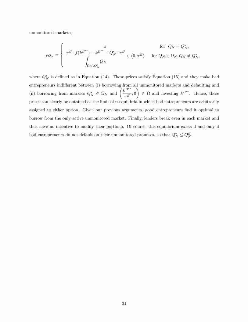
unmonitored markets,

=

⎧⎪⎪⎪⎨⎪⎪⎪⎩ for = ∗ ,

· (∗∗)− ∗∗ −∗ · Z

Ω\∗

∈ ¡0 ¢ for ∈ Ω 6= ∗ ,

where ∗ is defined as in Equation (14). These prices satisfy Equation (15) and they make bad

entrepreneurs indifferent between (i) borrowing from all unmonitored markets and defaulting and

(ii) borrowing from markets ∗ ∈ Ω and

µ

∗∗

0

¶∈ Ω and investing

∗∗. Hence, these

prices can clearly be obtained as the limit of -equilibria in which bad entrepreneurs are arbitrarily

assigned to either option. Given our previous arguments, good entrepreneurs find it optimal to

borrow from the only active unmonitored market. Finally, lenders break even in each market and

thus have no incentive to modify their portfolio. Of course, this equilibrium exists if and only if

bad entrepreneurs do not default on their unmonitored promises, so that ∗ ≤ .

34