Embed Size (px)
Citation preview
Communication Methods and Measures, 6:77–98, 2012Copyright © Taylor & Francis Group, LLCISSN: 1931-2458 print/1931-2466 onlineDOI: 10.1080/19312458.2012.679848
Advantages of Monte Carlo Confidence Intervalsfor Indirect Effects
Kristopher J. PreacherVanderbilt University
James P. SeligUniversity of New Mexico
Monte Carlo simulation is a useful but underutilized method of constructing confidence intervals forindirect effects in mediation analysis. The Monte Carlo confidence interval method has several dis-tinct advantages over rival methods. Its performance is comparable to other widely accepted methodsof interval construction, it can be used when only summary data are available, it can be used in situa-tions where rival methods (e.g., bootstrapping and distribution of the product methods) are difficult orimpossible, and it is not as computer-intensive as some other methods. In this study we discuss MonteCarlo confidence intervals for indirect effects, report the results of a simulation study comparing theirperformance to that of competing methods, demonstrate the method in applied examples, and discussseveral software options for implementation in applied settings.
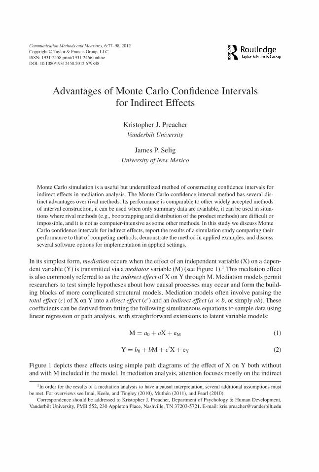
In its simplest form, mediation occurs when the effect of an independent variable (X) on a depen-dent variable (Y) is transmitted via a mediator variable (M) (see Figure 1).1 This mediation effectis also commonly referred to as the indirect effect of X on Y through M. Mediation models permitresearchers to test simple hypotheses about how causal processes may occur and form the build-ing blocks of more complicated structural models. Mediation models often involve parsing thetotal effect (c) of X on Y into a direct effect (c′) and an indirect effect (a × b, or simply ab). Thesecoefficients can be derived from fitting the following simultaneous equations to sample data usinglinear regression or path analysis, with straightforward extensions to latent variable models:
M = a0 + aX + eM (1)
Y = b0 + bM + c′X + eY (2)
Figure 1 depicts these effects using simple path diagrams of the effect of X on Y both withoutand with M included in the model. In mediation analysis, attention focuses mostly on the indirect
1In order for the results of a mediation analysis to have a causal interpretation, several additional assumptions mustbe met. For overviews see Imai, Keele, and Tingley (2010), Muthén (2011), and Pearl (2010).
Correspondence should be addressed to Kristopher J. Preacher, Department of Psychology & Human Development,Vanderbilt University, PMB 552, 230 Appleton Place, Nashville, TN 37203-5721. E-mail: [email protected]
Dow
nloa
ded
by [
VU
L V
ande
rbilt
Uni
vers
ity],
[K
rist
ophe
r Pr
each
er]
at 1
0:13
08
June
201
2
78 K. J. PREACHER AND J. P. SELIG
X Y
Ma b
c'
X Yc
FIGURE 1 A simple mediation model. X is the predictor, M the hypoth-esized mediator, and Y the outcome. Regression residuals are excludedfrom the diagram for simplicity.
effect ab, although many methodologists emphasize the need to also consider the coefficientsc and c′ in making this determination. In more complicated mediation models, such as modelswith multiple mediators, hierarchically clustered data, or longitudinal data, the indirect effectexpression will be correspondingly more complex.
In this article we discuss Monte Carlo (MC) confidence intervals for indirect effects. MCintervals capitalize on the fact that most statistics software packages provide the asymptoticcovariance matrix of the parameter estimates involved in indirect effects. A sampling distributionof the indirect effect can be simulated from this matrix, and percentiles of this distribution can beused to construct a confidence interval. We provide a small simulation study comparing the per-formance of MC confidence intervals to parametric, nonparametric, and residual-based bootstrapintervals, as well as intervals based on the delta method and distribution of products, demonstratethe method in two examples, and discuss several software options for implementation in appliedsettings.
METHODS FOR CONSTRUCTING CONFIDENCE INTERVALSFOR INDIRECT EFFECTS
Let θ be a generic population parameter whose value we wish to estimate. Chernick (2008)defines a 100(1 − α)% confidence interval (CI) for the value of θ in the following way:
“. . . if we construct a 95% confidence interval, we would expect that our procedure would produceintervals that contain the true parameter in 95% of the cases. Such is the definition of a confidenceinterval.” (p. 53)
Thus, a CI for θ may be defined in terms of the true (unknown) parameter value without referenceto any particular null hypothesis. A simple example of a confidence interval is a 95% CI for thepopulation mean of a normally distributed variable, expressed as CI.95 : {θ ± tcSEθ }, where tc isthe two-tailed critical value of the corresponding Student’s t distribution and SEθ is the standarderror of the estimate. With reference to the model in Figure 1, the indirect effect is most oftenquantified as the sample estimate ab. Various methods for constructing CIs for the parameter abdiffer only in how the sampling distribution of ab is obtained and used to gauge significance. Wenext describe the major methods of CI construction for indirect effects.
Delta Method
The delta method (DM) is a popular method for deriving the sampling variance of compoundstatistics like ab. This sampling variance, in turn, can be used in the construction of symmetric
Dow
nloa
ded
by [
VU
L V
ande
rbilt
Uni
vers
ity],
[K
rist
ophe
r Pr
each
er]
at 1
0:13
08
June
201
2
MONTE CARLO CONFIDENCE INTERVALS 79
confidence intervals. The method proceeds by first obtaining the asymptotic covariance matrix ofparameter estimates a and b, then pre- and post-multiplying by the vector-valued derivative (D)of the Taylor series expansion of ab with respect to each of these parameters evaluated at theirmeans. The result is a scalar approximation to the sampling variance of ab where s2
band s2
a are
the estimated sampling variances of a and b, respectively:
var[ab] ≈ a2s2b+ b2s2
a (3)
The square root of this sampling variance is often used as a standard error in significance tests forthe indirect effect (Sobel, 1982) or to construct a symmetric confidence interval for ab:
CI1−α = ab ± zα/2
√var[ab] (4)
Unfortunately, ab is not normally distributed, although it may approach normality in large sam-ples (Aroian, 1947; Craig, 1936). In most cases, the distribution of ab is skewed and leptokurtic(Bollen & Stine, 1990; MacKinnon, Lockwood, Hoffman, West, & Sheets, 2002; MacKinnon,Lockwood, & Williams, 2004). When the assumption of normality is not tenable, intervals basedon the delta method are not appropriate in the majority of cases. Nevertheless, the delta methodis the default method most commonly included in structural equation modeling (SEM) softwarefor obtaining tests and CIs for indirect effects.
Distribution of the Product Method
The distribution of the product (DP) strategy considers the correct distribution of ab rather thanassuming that it is normal or approximating it in some way. To use the DP method, researchersare obliged to convert a and b to z-scores, form the product zazb, and compare the result toa table of critical values (MacKinnon et al., 2004; Meeker, Cornwell, & Aroian, 1981). Thismethod performs well in simulation studies, but until recently required recourse to tables withlimited availability and knowledge of the population value of either a or b. The first of theselimitations has been overcome with the availability of PRODCLIN (available in Fortran, SAS,SPSS, and R formats; MacKinnon, Fritz, Williams, & Lockwood, 2007), a program that can beused to construct asymmetric confidence limits using the distribution of the product approach.The second limitation cannot be circumvented but becomes less relevant as N increases.
Nonparametric Percentile Bootstrap and Corrections
Bootstrapping (Efron, 1982; Efron & Tibshirani, 1993) is a nonparametric resampling methodthat involves generating an empirical sampling distribution of ab and using it as a basis for statis-tical estimation and inference. An arbitrarily large number (B) of resamples of size N are sampledindependently with replacement from the original sample. The product ab∗ is estimated for eachof these B resamples, resulting in an empirical sampling distribution of ab∗. Percentile-based(PC) confidence intervals (Efron, 1981) may be constructed for any degree of precision by iden-tifying the values of ab∗ corresponding to the lower and upper 50α% of the distribution. Thesevalues define the limits of a 100(1 − α)% asymmetric CI about the sample ab.
Dow
nloa
ded
by [
VU
L V
ande
rbilt
Uni
vers
ity],
[K
rist
ophe
r Pr
each
er]
at 1
0:13
08
June
201
2

80 K. J. PREACHER AND J. P. SELIG
Efron (1981, 1982, 1987) and Efron and Tibshirani (1986, 1993) suggest adjustments thatreduce bias in percentile bootstrap interval bounds. Whereas percentile bounds are taken directlyfrom the desired percentiles of the empirical sampling distribution of ab∗, bias-corrected (BC)bounds incorporate an adjustment. Letting z0 be the z-score corresponding to the proportion ofthe B bootstrap resamples with ab∗ less than the estimated sample ab, two z-scores are definedas:
z′lower = 2z0 + zα/2 (5)
z′upper = 2z0 + z1−α/2 (6)
The proportions under the standard normal distribution that correspond to z′lower and z′
upper are mul-tiplied by 100 to serve as the adjusted percentiles for selecting interval limits from the bootstrapdistribution of ab∗. The BC bootstrap has been found to perform well in terms of Type I errorrates and statistical power when testing indirect effects (MacKinnon et al., 2004). However, it hasbeen observed that BC limits do not always have good coverage (Schenker, 1985); that is, acrossrepeated sampling, BC intervals do not necessarily include the population parameter the desiredpercentage of times. This in part motivated the creation of bias-corrected and accelerated (BCa)confidence limits (Efron, 1987). BCa percentiles include further adjustment by an accelerationconstant a:
z′lower = z0 + z0 + zα/2
1 − a(z0 + zα/2
) (7)
z′upper = z0 + z0 + z1−α/2
1 − a(z0 + z1−α/2
) (8)
where a is approximately 1/6 of the skewness of the bootstrap distribution of ab∗. Thus, 2z0
is a correction for median bias and a is a correction for skewness (DiCiccio & Efron, 1996;Efron & Tibshirani, 1986, 1993). BCa confidence limits are second-order accurate in many caseswhere estimators can be expressed as functions of multivariate vector means (e.g., indirect effects)(DiCiccio & Romano, 1988; Efron, 1987, p. 176; Efron & Tibshirani, 1993; Hall, 1989), mean-ing that coverage rates approach the nominal value very quickly as N increases. In theory, BCaintervals offer an improvement over BC intervals, but in practice the superiority of one type ofinterval over the other can depend on the context.
The primary benefits of bootstrapping are that it involves no distributional assumptions andcan be used in small samples. Unlike DM intervals, bootstrap intervals for ab are asymmet-ric, resembling more closely the true distribution of products, which tends to be somewhatskewed away from zero (Bollen & Stine, 1990). The only apparent drawbacks to the boot-strap include slight inconsistency among replications of the same experiment with the samedata due to random resampling variability and the time commitment due to computer-intensiveresampling.
Bootstrapping has been found to perform well relative to other methods of CI construction forindirect effects (Bollen & Stine, 1990; Efron & Tibshirani, 1993; Lockwood & MacKinnon, 1998;
Dow
nloa
ded
by [
VU
L V
ande
rbilt
Uni
vers
ity],
[K
rist
ophe
r Pr
each
er]
at 1
0:13
08
June
201
2
MONTE CARLO CONFIDENCE INTERVALS 81
MacKinnon et al., 2004; Preacher & Hayes, 2004; Shrout & Bolger, 2002). Hypothesis tests basedon BC and BCa intervals have fairly accurate Type I error rates and higher power when comparedto competing methods used to test null hypotheses about indirect effects. Fritz and MacKinnon(2007) demonstrated that, of several competing methods, BC required the smallest N to achievecomparable levels of power. On the other hand, Fritz and MacKinnon (2007), Fritz, Taylor, andMacKinnon (2012), and MacKinnon et al. (2004) report that BC and BCa bootstrap CIs yieldtoo-high Type I error rates in some conditions when N is small, and Polansky (1999) reports poorCI coverage in very small samples. Biesanz, Falk, and Savalei (2010) found that BCa intervals didnot perform as well as PC intervals. Bootstrap methods are available for estimating indirect effectsin some SEM software applications and in macros for use in SPSS and SAS (Cheung, 2007;Lockwood & MacKinnon, 1998; Preacher & Hayes, 2004, 2008; Preacher, Rucker, & Hayes,2007; Shrout & Bolger, 2002).
Residual-Based Bootstrap
Residual-based bootstrapping (RB) is often used with regression models in which the designmatrix is considered fixed, which includes most applications of regression (Efron, 1979; Efron& Tibshirani, 1993; Freedman, 1981; Stine, 1989). It has been adapted for use in multilevelmodeling where there is no clearly superior way to employ more traditional bootstrap methods(van der Leeden, Meijer, & Busing, 2008; Wang, Carpenter, & Kepler, 2006). In the regression orSEM context, the first step in residual-based bootstrapping is to estimate the regression weightsor path coefficients and compute observed residuals (eM) according to, for example, Equation 1.The second step is to bootstrap the residuals. The resampled residuals are then added to the fittedequation a0 + aX to generate bootstrap values of the mediator M∗. These, in turn, are regressedonto the fixed X to produce a bootstrapped value of a∗. This process is repeated B times togenerate a bootstrapped distribution of a∗, where B is large (several thousand). In adapting themethod to the simple mediation context, there are two residuals to resample: those for the Mequation and those for the Y equation (Zhang & Wang, 2008). For simple mediation models, pairsof residuals (eM,eY) are obtained from Equations 1 and 2 fit to the observed data. Residual pairsare then bootstrapped from this joint distribution and added (respectively) to the fitted equationsa0 + aX and b0 + bM + c′X to yield bootstrapped values of both M∗ and Y∗. M∗ is regressedon the fixed X to yield a∗, whereas Y∗ is regressed on the fixed X and the random M∗ to yieldb∗. This process is repeated B times to generate a bootstrap distribution of ab∗. The empiricalsampling distribution of ab∗ can be used in the usual way to form PC, BC, or BCa CIs. Zhang andWang (2008) note that RB bootstrap requires errors to be independent and identically distributed(iid), an assumption not required for other bootstrapping methods. They found that RB bootstrapCIs have good coverage and power for medium to large effects when residuals are iid. Whenresiduals are heterogeneous, the RB bootstrap performed better with small effect size whereasthe PC bootstrap performed better with large effect sizes.
The RB bootstrap has been used to assess mediation in multilevel models (Pituch, Stapleton,& Kang, 2006) but has only recently been suggested for use in the more common single-levelmediation models (Zhang & Wang, 2008). The version of the RB bootstrap used in our simulationis identical to that of Zhang and Wang and similar to that of Pituch et al., except that residualswere obtained via bootstrapping rather than through Monte Carlo simulation. Zhang and Wangprovide software (MedCI) for computing confidence limits using the RB bootstrap.
Dow
nloa
ded
by [
VU
L V
ande
rbilt
Uni
vers
ity],
[K
rist
ophe
r Pr
each
er]
at 1
0:13
08
June
201
2

82 K. J. PREACHER AND J. P. SELIG
Parametric Bootstrap
The parametric bootstrap (PB) method can be traced to Efron (1980, 1982; Efron & Tibshirani,1986, 1993), and is sometimes called parametric simulation (Davison & Hinkley, 1997). ThePB method relies on the assumption that the parameters a and b have a known joint samplingdistribution, not necessarily normal, with parameters supplied by (often, but not necessarily)maximum likelihood estimates from the fitted parametric model. The model, with parame-ter estimates treated as parameters, is used to repeatedly generate bootstrap resamples. Forexample, the model-implied covariance matrix in a linear path model might be used as a pop-ulation matrix, from which sample data matrices could be generated (e.g., using the methodof Kaiser and Dickman [1962]). The statistic of interest (θ ), which may be a simple or com-plex function of other model statistics, is computed in each resample. Thus, in contrast to thenonparametric bootstrap, in which bootstrap data consist of resampled cases from the originalsample, in the parametric bootstrap the bootstrap data are generated parametrically from a fit-ted model. Percentiles of the sampling distribution of θ are identified to serve as limits for a100(1 − α)% asymmetric confidence interval about the sample θ , where θ = ab in mediationanalysis. Bias correction, with or without acceleration, may be used just as with the nonparametricbootstrap.
Generation of the parametrically simulated data can proceed in a number of ways, typically byemploying software-based pseudorandom number generation. Even though parametric assump-tions are invoked for a and b, no parametric assumptions are made about the distribution of ab.The advantages of the PB method include most of those associated with nonparametric bootstrapCIs—the intervals are properly asymmetric, and are useful in situations where obtaining CIs byanalytic means is difficult or impossible. An advantage over the nonparametric bootstrap is thatthe PB method is not limited to using case data that were actually observed in one’s empiricallyobtained sample; data are generated parametrically, which implies that the sampling distribu-tion of ab will be smoother. This becomes important especially when high confidence levels aredesired (e.g., 99%), the sample is small (Davison & Hinkley, 1997), and/or the sampling distri-bution is heavily skewed. Furthermore, the PB method can be used when only summary data areavailable, facilitating re-analysis or meta-analysis. A disadvantage is that it is necessary to makesome possibly unwarranted parametric distributional assumptions at the data simulation stage.The procedure will yield biased results to the extent that the original point estimates and theirasymptotic (co)variances are affected by model misspecification.
Accessible discussions of the PB method can be found in Chernick (2008, pp. 124–125),Davison and Hinkley (1997, pp. 15–21), Efron (1980, pp. 40–41; 1982, pp. 29–30; 1986,pp. 56–57), and Efron and Tibshirani (1993, pp. 53–56). The PB method is implemented in the Rcommand “boot” using sim=“parametric” (Davison & Hinkley, pp. 528–529).
The Monte Carlo Method
The Monte Carlo (MC) method involves generating a sampling distribution of a compound statis-tic by using point estimates of its component statistics, along with the asymptotic covariancematrix of these estimates and assumptions about how the component statistics are distributed.
Dow
nloa
ded
by [
VU
L V
ande
rbilt
Uni
vers
ity],
[K
rist
ophe
r Pr
each
er]
at 1
0:13
08
June
201
2

MONTE CARLO CONFIDENCE INTERVALS 83
For example, a sampling distribution for the ratio of two independent means could be gen-erated by first fitting a model to empirical data and obtaining point estimates and asymptoticvariances for the means. Because means are asymptotically normal according to the CentralLimit Theorem, a large number of random draws could be taken from a bivariate normal dis-tribution of the means, each time creating the ratio θ∗ = x∗
1/x∗2, yielding a sampling distribution
of the ratio. A CI can then be formed on the basis of this sampling distribution in the sameway as bootstrap intervals. However, in contrast to bootstrap methods, the MC method involvesdirectly generating sample statistics from their joint asymptotic distribution, not resampling orgenerating data.
The MC method was first applied to the mediation context by MacKinnon et al. (2004) and isclosely related to the empirical-M method (MacKinnon et al., 2002, 2004; Pituch & Stapleton,2008; Pituch et al., 2006; Pituch, Whittaker, & Stapleton, 2005), especially as generalized byWilliams and MacKinnon (2008) to cases beyond single-mediator models. The MC method relieson the assumption that the parameters a and b have a joint normal sampling distribution, withparameters supplied by (often, but not necessarily) maximum likelihood estimates from the fittedparametric model:
[a∗b∗
]∼ MVN
([ab
],
[σ 2
a σabσab σ 2
b
])(9)
In the traditional three-variable mediation model of Figure 1, σab is often replaced with 0 forsimplicity. Using the parametric assumption in (9), a sampling distribution of ab is formed byrepeatedly generating a∗ and b∗ and computing their product. Values for a and b can be gener-ated in a number of ways, most often using software-based pseudorandom number generation.Parametric assumptions are invoked for a and b, but no parametric assumptions are made aboutthe distribution of ab. Even though parametric assumptions are invoked for a and b, no paramet-ric assumptions are made about the distribution of ab. Percentiles of this sampling distributionare identified to serve as limits for a 100(1 − α)% asymmetric confidence interval about thesample ab.
Advantages of the MC method include most of those associated with nonparametric bootstrapCIs (e.g., asymmetry, usefulness in otherwise intractable situations). It also shares the advan-tage of the PB method in that the sampling distribution of ab can be made arbitrarily smoothas B increases, and it can be used when only summary data are available. The MC method hasa unique advantage over bootstrap methods in that it is very fast; the model is fit to data onlyonce. This can be a huge advantage when using models that take a long time to converge. TheMC method can be used in situations where bootstrapping is not feasible, such as multilevelmodeling, when samples are so small that bootstrapping may randomly generate a constant vari-able and stop, or when distinct values of a variable are limited and highly unbalanced (as inresearch on rare disorders). MacKinnon et al. (2004) found MC CIs to show performance sim-ilar to the PC bootstrap and inferior to BC bootstrap CIs. Thus, if the MC method is found toperform similarly to (or not significantly worse than) bootstrap methods and the DP method,we argue that researchers should give it serious consideration as a viable alternative to thesemethods.
Dow
nloa
ded
by [
VU
L V
ande
rbilt
Uni
vers
ity],
[K
rist
ophe
r Pr
each
er]
at 1
0:13
08
June
201
2
84 K. J. PREACHER AND J. P. SELIG
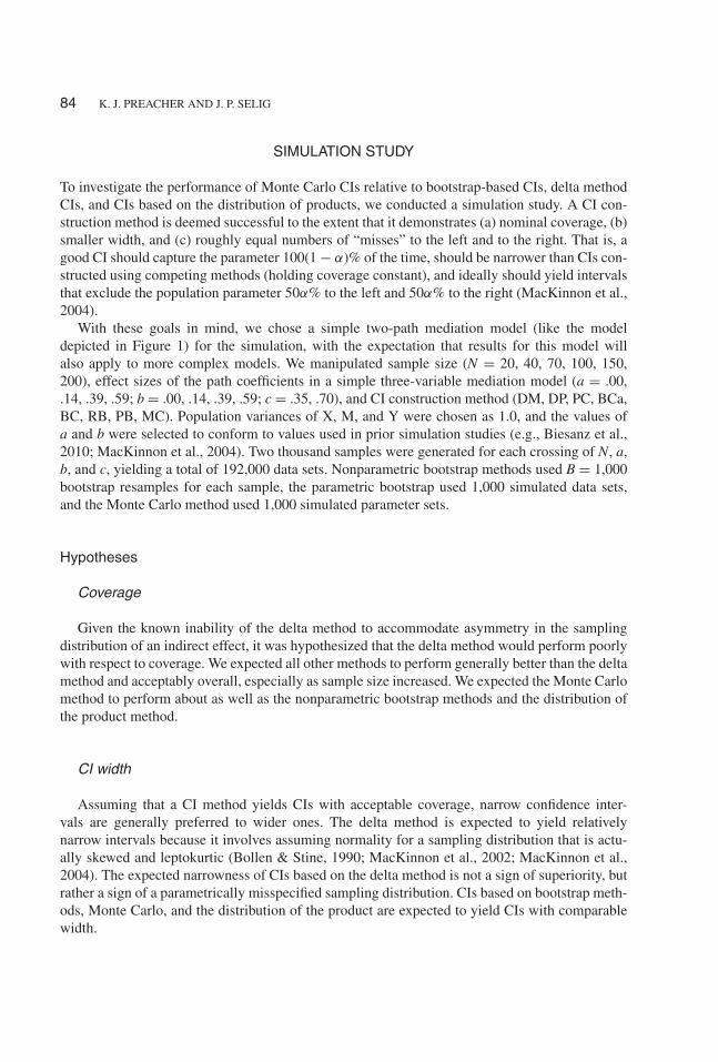
SIMULATION STUDY
To investigate the performance of Monte Carlo CIs relative to bootstrap-based CIs, delta methodCIs, and CIs based on the distribution of products, we conducted a simulation study. A CI con-struction method is deemed successful to the extent that it demonstrates (a) nominal coverage, (b)smaller width, and (c) roughly equal numbers of “misses” to the left and to the right. That is, agood CI should capture the parameter 100(1 − α)% of the time, should be narrower than CIs con-structed using competing methods (holding coverage constant), and ideally should yield intervalsthat exclude the population parameter 50α% to the left and 50α% to the right (MacKinnon et al.,2004).
With these goals in mind, we chose a simple two-path mediation model (like the modeldepicted in Figure 1) for the simulation, with the expectation that results for this model willalso apply to more complex models. We manipulated sample size (N = 20, 40, 70, 100, 150,200), effect sizes of the path coefficients in a simple three-variable mediation model (a = .00,.14, .39, .59; b = .00, .14, .39, .59; c = .35, .70), and CI construction method (DM, DP, PC, BCa,BC, RB, PB, MC). Population variances of X, M, and Y were chosen as 1.0, and the values ofa and b were selected to conform to values used in prior simulation studies (e.g., Biesanz et al.,2010; MacKinnon et al., 2004). Two thousand samples were generated for each crossing of N, a,b, and c, yielding a total of 192,000 data sets. Nonparametric bootstrap methods used B = 1,000bootstrap resamples for each sample, the parametric bootstrap used 1,000 simulated data sets,and the Monte Carlo method used 1,000 simulated parameter sets.
Hypotheses
Coverage
Given the known inability of the delta method to accommodate asymmetry in the samplingdistribution of an indirect effect, it was hypothesized that the delta method would perform poorlywith respect to coverage. We expected all other methods to perform generally better than the deltamethod and acceptably overall, especially as sample size increased. We expected the Monte Carlomethod to perform about as well as the nonparametric bootstrap methods and the distribution ofthe product method.
CI width
Assuming that a CI method yields CIs with acceptable coverage, narrow confidence inter-vals are generally preferred to wider ones. The delta method is expected to yield relativelynarrow intervals because it involves assuming normality for a sampling distribution that is actu-ally skewed and leptokurtic (Bollen & Stine, 1990; MacKinnon et al., 2002; MacKinnon et al.,2004). The expected narrowness of CIs based on the delta method is not a sign of superiority, butrather a sign of a parametrically misspecified sampling distribution. CIs based on bootstrap meth-ods, Monte Carlo, and the distribution of the product are expected to yield CIs with comparablewidth.
Dow
nloa
ded
by [
VU
L V
ande
rbilt
Uni
vers
ity],
[K
rist
ophe
r Pr
each
er]
at 1
0:13
08
June
201
2

MONTE CARLO CONFIDENCE INTERVALS 85
Misses
Ideally, a CI should exclude the parameter to an equal degree to the left and right; that is,it should be symmetric with respect to misses. To operationalize this symmetry, we computedthe ratio of right-side misses to left-side misses. A value of 1 indicates perfect symmetry withrespect to missing the population indirect effect, whereas departures from 1 indicate imbalance.We expected the delta method to yield unbalanced misses due to its artificially symmetric CIs. Weexpected Monte Carlo methods to perform on par with bootstrap and distribution of the productmethods.
Overall, it was our expectation that the Monte Carlo method would perform acceptably on allcounts when compared to bootstrap methods and the distribution of the product method. If theMonte Carlo method is comparable to (or not much worse than) existing methods for constructingasymmetric CIs, we argue that this method presents a useful alternative to these other methodswhen raw data are unavailable.
Results
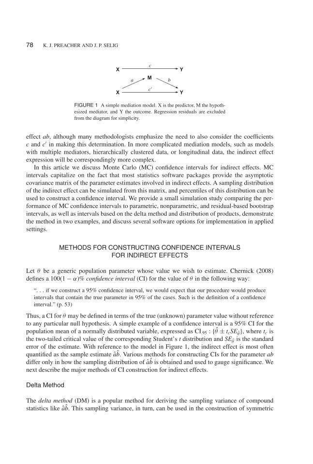
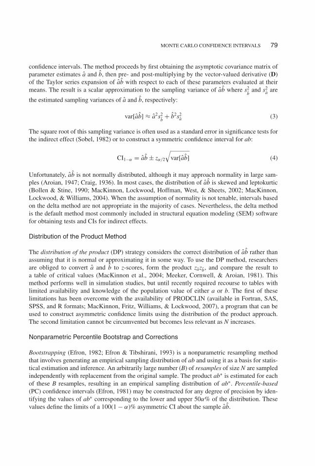
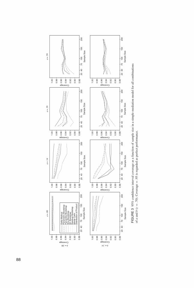
Coverage
Coverage is reported for all cells of the design in Figure 2 (for c = .35) and Figure 3 (forc = .70). Overall, results were comparable for c = .35 and c = .70, and results for the BC andBCa bootstrap methods were virtually indistinguishable. As predicted, the delta method tendedto have coverage that was too high in some conditions, mainly when either a or b was small.As a and b increased, and as sample size increased, most methods converged on .95. The MonteCarlo method appeared to perform comparably to the parametric, percentile, and residual-basedbootstrap methods. To better quantify coverage, we computed the average root mean squarederror (RMSE) of observed CI coverage (with respect to the nominal .95 level) across all a, b, andN conditions (but separately for c = .35 and c = .70). Results, reported in Table 1, demonstratethat the Monte Carlo method was among the best methods in terms of coverage—as good as,or slightly better than—the parametric, percentile, and residual-based bootstrap methods and thedistribution of the product method.
CI width
Summary results for interval width are reported in Table 1. Averaging across all conditions,the delta method showed the narrowest intervals (average width = .233), although this narrow-ness is of questionable worth given its relatively poor coverage. Among the remaining methodswith acceptable coverage, the distribution of the product method had the narrowest CIs (.236),followed by the Monte Carlo method (.249).
Misses
The ratio of average right-side misses to average left-side misses is reported for all methods inTable 1. All methods demonstrated more average misses to the right than to the left (keeping in
Dow
nloa
ded
by [
VU
L V
ande
rbilt
Uni
vers
ity],
[K
rist
ophe
r Pr
each
er]
at 1
0:13
08
June
201
2

Sam
ple
Siz
e
2040
7010
015
020
0
Sam
ple
Siz
e20
4070
100
150
200
Sam
ple
Siz
e20
4070
100
150
200
Sam
ple
Siz
e
2040
7010
015
020
0
Sam
ple
Siz
e
2040
7010
015
020
0
Sam
ple
Siz
e20
4070
100
150
200
Sam
ple
Siz
e
2040
7010
015
020
0
Coverage
0.88
0.90
0.92
0.94
0.96
0.98
1.00
Del
ta M
etho
dP
aram
etric
Boo
tstr
apP
erce
ntile
Boo
tstr
apB
Ca
Boo
tstr
apB
C B
oots
trap
Res
idua
l Boo
tstr
apM
onte
Car
loD
istr
ibut
ion
of P
rodu
ct
Coverage
0.88
0.90
0.92
0.94
0.96
0.98
1.00
Coverage
0.88
0.90
0.92
0.94
0.96
0.98
1.00
Coverage
0.88
0.90
0.92
0.94
0.96
0.98
1.00
Coverage
0.88
0.90
0.92
0.94
0.96
0.98
1.00
Coverage
0.88
0.90
0.92
0.94
0.96
0.98
1.00
Coverage
0.88
0.90
0.92
0.94
0.96
0.98
1.00
Coverage
0.88
0.90
0.92
0.94
0.96
0.98
1.00
b = .00
a =
.00
a =
.14
b = .14
a =
.39
a =
.59
Sam
ple
Siz
e
2040
7010
015
020
0
FIG
UR
E2
95%
confi
denc
ein
terv
alco
vera
geas
afu
nctio
nof
sam
ple
size
ina
sim
ple
med
iatio
nm
odel
for
allc
ombi
natio
nsof
aan
db
(c=
.35)
.Cov
erag
e=
.95
isre
gard
edas
perf
ectp
erfo
rman
ce.
86
Dow
nloa
ded
by [
VU
L V
ande
rbilt
Uni
vers
ity],
[K
rist
ophe
r Pr
each
er]
at 1
0:13
08
June
201
2

Coverage
0.88
0.90
0.92
0.94
0.96
0.98
1.00
Coverage
0.88
0.90
0.92
0.94
0.96
0.98
1.00
Coverage
0.88
0.90
0.92
0.94
0.96
0.98
1.00
Coverage
0.88
0.90
0.92
0.94
0.96
0.98
1.00
Coverage
0.88
0.90
0.92
0.94
0.96
0.98
1.00
Coverage
0.88
0.90
0.92
0.94
0.96
0.98
1.00
Coverage
0.88
0.90
0.92
0.94
0.96
0.98
1.00
Coverage
0.88
0.90
0.92
0.94
0.96
0.98
1.00
b = .59 b = .39
Sam
ple
Siz
e20
4070
100
150
200
Sam
ple
Siz
e20
4070
100
150
200
Sam
ple
Siz
e
2040
7010
015
020
0
Sam
ple
Siz
e
2040
7010
015
020
0
Sam
ple
Siz
e
2040
7010
015
020
0
Sam
ple
Siz
e
2040
7010
015
020
0
Sam
ple
Siz
e
2040
7010
015
020
0
Sam
ple
Siz
e20
4070
100
150
200
FIG
UR
E2
(Con
tinu
ed).
87
Dow
nloa
ded
by [
VU
L V
ande
rbilt
Uni
vers
ity],
[K
rist
ophe
r Pr
each
er]
at 1
0:13
08
June
201
2
Sam
ple
Siz
e20
4070
100
150
200
Sam
ple
Siz
e
2040
7010
015
020
0
Sam
ple
Siz
e20
4070
100
150
200
Sam
ple
Siz
e
2040
7010
015
020
0
Sam
ple
Siz
e20
4070
100
150
200
Sam
ple
Siz
e20
4070
100
150
200
Sam
ple
Siz
e20
4070
100
150
200
Sam
ple
Siz
e20
4070
100
150
200
Coverage
0.88
0.90
0.92
0.94
0.96
0.98
1.00
Del
ta M
etho
dP
aram
etric
Boo
tstr
apP
erce
ntile
Boo
tstr
apB
Ca
Boo
tstr
apB
C B
oots
trap
Res
idua
l Boo
tstr
apM
onte
Car
loD
istr
ibut
ion
of P
rodu
ct
Coverage
0.88
0.90
0.92
0.94
0.96
0.98
1.00
Coverage
0.88
0.90
0.92
0.94
0.96
0.98
1.00
Coverage
0.88
0.90
0.92
0.94
0.96
0.98
1.00
Coverage
0.88
0.90
0.92
0.94
0.96
0.98
1.00
Coverage
0.88
0.90
0.92
0.94
0.96
0.98
1.00
Coverage
0.88
0.90
0.92
0.94
0.96
0.98
1.00
Coverage
0.88
0.90
0.92
0.94
0.96
0.98
1.00
b = .00 b = .14
a =
.00
a =
.14
a =
.39
a =
.59
FIG
UR
E3
95%
confi
denc
ein
terv
alco
vera
geas
afu
nctio
nof
sam
ple
size
ina
sim
ple
med
iatio
nm
odel
for
allc
ombi
natio
nsof
aan
db
(c=
.70)
.Cov
erag
e=
.95
isre
gard
edas
perf
ectp
erfo
rman
ce.
88
Dow
nloa
ded
by [
VU
L V
ande
rbilt
Uni
vers
ity],
[K
rist
ophe
r Pr
each
er]
at 1
0:13
08
June
201
2

Coverage
0.88
0.90
0.92
0.94
0.96
0.98
1.00
Coverage
0.88
0.90
0.92
0.94
0.96
0.98
1.00
Coverage
0.88
0.90
0.92
0.94
0.96
0.98
1.00
Coverage
0.88
0.90
0.92
0.94
0.96
0.98
1.00
Coverage
0.88
0.90
0.92
0.94
0.96
0.98
1.00
Coverage
0.88
0.90
0.92
0.94
0.96
0.98
1.00
Coverage
0.88
0.90
0.92
0.94
0.96
0.98
1.00
Coverage
0.88
0.90
0.92
0.94
0.96
0.98
1.00
b = .39 b = .59
Sam
ple
Siz
e20
4070
100
150
200
Sam
ple
Siz
e20
4070
100
150
200
Sam
ple
Siz
e
2040
7010
015
020
0
Sam
ple
Siz
e
2040
7010
015
020
0
Sam
ple
Siz
e20
4070
100
150
200
Sam
ple
Siz
e20
4070
100
150
200
Sam
ple
Siz
e20
4070
100
150
200
Sam
ple
Siz
e20
4070
100
150
200
FIG
UR
E3
(Con
tinu
ed).
89
Dow
nloa
ded
by [
VU
L V
ande
rbilt
Uni
vers
ity],
[K
rist
ophe
r Pr
each
er]
at 1
0:13
08
June
201
2
90 K. J. PREACHER AND J. P. SELIG
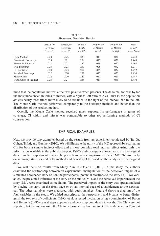
TABLE 1Abbreviated Simulation Results
RMSE for RMSE for Overall Proportion Proportion Right-Coverage Coverage Width of Misses of Misses to-Left(c = .35) (c = .70) for CIs to Left to Right Miss Ratio
Delta Method .028 .025 .233 .011 .030 2.743Parametric Bootstrap .023 .021 .259 .015 .022 1.449Percentile Bootstrap .021 .021 .252 .019 .027 1.467BCa Bootstrap .023 .023 .257 .025 .032 1.271BC Bootstrap .023 .023 .257 .025 .032 1.272Residual Bootstrap .022 .020 .252 .017 .025 1.450Monte Carlo .022 .020 .249 .017 .025 1.447Distribution of Product .023 .021 .236 .019 .031 1.670
mind that the population indirect effect was positive when present). The delta method was by farthe most unbalanced in terms of misses, with a right-to-left ratio of 2.743; that is, the populationab was nearly three times more likely to be excluded to the right of the interval than to the left.The Monte Carlo method performed comparably to the bootstrap methods and better than thedistribution of the product method.
Overall, the Monte Carlo method received much support. Its performance in terms ofcoverage, CI width, and misses was comparable to other top-performing methods of CIconstruction.
EMPIRICAL EXAMPLES
Next we provide two examples based on the results from an experiment conducted by Tal-Or,Cohen, Tsfati, and Gunther (2010). We will illustrate the utility of the MC approach by estimatingCIs for both a simple indirect effect and a more complex total indirect effect using only theinformation available in the published report. Tal-Or and colleagues allowed us to use the originaldata from their experiment so it will be possible to make comparisons between MC CIs based onlyon summary statistics and delta method and bootstrap CIs based on the analysis of the originaldata.
We will focus on results from Study 2 in Tal-Or et al. (2010). In this study, the authorsexamined the relationship between an experimental manipulation of the perceived impact of asimulated newspaper story (X) on the participants’ potential reactions to the story (Y). Two vari-ables, the presumed influence of the story on the public (M1), and the perceived importance of thestory (M2), were examined as mediators. The perceived impact of the story was operationalizedby placing the story on the front page or on an internal page of a supplement to the newspa-per. The other variables were measured with questionnaires. Figure 4 shows a diagram of thefour variables in the study. We added subscripts to the respective a and b paths to better distin-guish the two sets of coefficients. Tal-Or et al. assessed mediation using a combination of Baronand Kenny’s (1986) causal steps approach and bootstrap confidence intervals. The CIs were notreported, but the authors used the CIs to determine that both indirect effects depicted in Figure 4
Dow
nloa
ded
by [
VU
L V
ande
rbilt
Uni
vers
ity],
[K
rist
ophe
r Pr
each
er]
at 1
0:13
08
June
201
2

MONTE CARLO CONFIDENCE INTERVALS 91
(i.e., perceived impact→media influence→potential reactions and perceived impact→perceivedimportance→potential reactions) were statistically significant (p < .05).
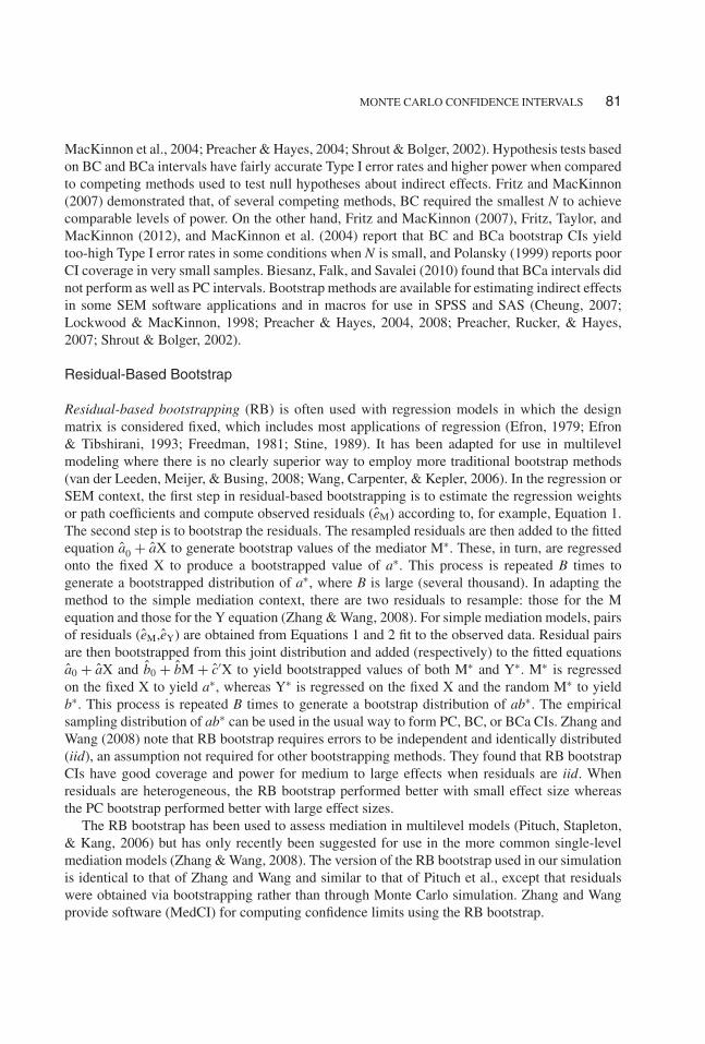
For the example of simple mediation, we will examine the effect of perceived impact on poten-tial reactions as mediated by presumed media influence. Tal-Or and colleagues report both thecoefficients and standard errors for this indirect effect (a1 = 0.48, SEa1 = 0.24; b1 = 0.40,SEb1 = 0.09). We entered these summary statistics into a web-based Monte Carlo calculator(Selig & Preacher, 2008) available at the website of the first author to compute a 95% CI basedon 20,000 simulated draws from the distributions for the a1 and b1 parameters. Figure 5 shows asimulated sampling distribution for the indirect effect (a1b1). This histogram is automatically gen-erated when computing MC CIs using the web-based calculator. The histogram shows a degree ofpositive skew consistent with the aforementioned nonnormal shape of distributions of products.
PotentialReactions
PerceivedImpact
MediaInfluence
PerceivedImportance
a2a2
a1 b1
b2
FIGURE 4 Diagram of the model from Tal-Or et al. (2010).
Distribution of Indirect Effect
95 % Confidence Interval LL 0.003838 UL 0.4225
Fre
quen
cy
–0.2 0.0 0.2 0.4 0.6 0.8
020
040
060
080
0
FIGURE 5 Simulated sampling distribution for the indirect effect (a1b1).
Dow
nloa
ded
by [
VU
L V
ande
rbilt
Uni
vers
ity],
[K
rist
ophe
r Pr
each
er]
at 1
0:13
08
June
201
2

92 K. J. PREACHER AND J. P. SELIG
TABLE 295% Confidence Intervals for the Indirect Effectof the Manipulation on Reactions as Mediated
by Media Influence
95% CIs for Indirect Effect(a1b1 = 0.189)
Method LL UL
Monte Carlo 0.004 0.423Delta Method −0.015 0.393Percentile Bootstrap 0.006 0.415Bias-Corrected Bootstrap 0.016 0.436
Next we used Mplus (Muthén & Muthén, 1998–2010) to conduct a path analysis of the vari-ables in Figure 4. For the path analysis we requested three different kinds of 95% CIs that Mpluscan produce. These three are based on: the delta method, the percentile bootstrap, and the biascorrected bootstrap. For this analysis we used 20,000 bootstrap resamples to compute the CIs.Table 2 shows the 95% CIs from all analyses. As can be seen from the 95% CIs in Table 2, allintervals except for the symmetric CI based on the delta method exclude zero. Therefore, theauthors’ conclusion regarding the evidence for mediation would be similar when using the MCapproach or either bootstrapping approach. The lower limit for the MC interval is lower than thatfor the two bootstrap CIs.
Next we used the same data to examine an indirect effect not considered by Tal-Or et al.(2010). This is the total indirect effect of perceived impact (X) on potential reactions (Y). Thetotal indirect effect describes all of the influence perceived impact had on potential reactions asmediated by both perceived media influence (M1) and perceived importance (M2). The estimate ofthe total indirect effect can be calculated as follows: (a1b1) + (a2b2). MacKinnon (2008) providesthe following delta method formula for the standard error for such a total indirect effect:
sa1b1+a2b2=
√s2
a1b2
1 + s2b1
a21 + s2
a2b2
2 + s2b2
a22 + 2a1a2sb1b2
+ 2b1b2sa1a2 (10)
Here sa1a2 and sb1b2describe the sample covariances between the two a parameter estimates and
the two b parameter estimates, respectively.Some SEM software packages such as Mplus allow the user to define new parameters that are
functions of other model parameters. The software can then provide both estimates and standarderrors for the new parameters. In this way, one could define the total indirect effect above as a newparameter and calculate a standard error and/or CI for the total indirect effect. In many situationsit is also possible to use the MC approach to estimate CIs for the total indirect effect. This is doneby simulating random draws from the distributions for the four parameters involved in the totalindirect effect (i.e., a1, b1, a2, b2).
When using path analysis, there is no assumption that the parameter covariances are equal tozero, so it is possible that the four parameters that constitute the total indirect effect may havenonzero covariances. As can be seen in Equation 10, these covariances are needed to compute thestandard error and are also important for the MC approach. In other words, it may be necessary
Dow
nloa
ded
by [
VU
L V
ande
rbilt
Uni
vers
ity],
[K
rist
ophe
r Pr
each
er]
at 1
0:13
08
June
201
2
MONTE CARLO CONFIDENCE INTERVALS 93
to sample values of the coefficients from a multivariate normal distribution using the covariancematrix of the parameters as a population covariance matrix.
When it is necessary to know about the covariances of the parameter estimates constituting anindirect effect, there are two options available in addition to access to raw data. The first optionrequires the authors to report the asymptotic covariance matrix (ACM) of the parameter estimates,which can be obtained in most regression and SEM packages. Given current reporting norms, webelieve this will be a rare occurrence. The second option requires the authors to report the covari-ance matrix for the variables used in the analysis. It is then possible to use the covariance matrixin an SEM software package to replicate the analyses in the report. Many software packages willthen give the user the option of outputting the ACM. This covariance matrix can then be used tosimulate random values from a multivariate normal distribution of the parameters.
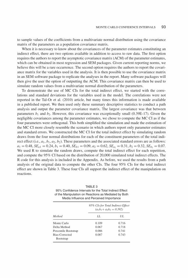
To demonstrate the use of MC CIs for the total indirect effect, we started with the corre-lations and standard deviations for the variables used in the model. The correlations were notreported in the Tal-Or et al. (2010) article, but many times this information is made availablein a published report. We then used only these summary descriptive statistics to conduct a pathanalysis and output the parameter covariance matrix. The largest covariance was that betweenparameters b1 and b2. However, this covariance was exceptionally small (0.39E-17). Given thenegligible covariances among the parameter estimates, we chose to compute the MC CI as if thefour parameters were orthogonal. This both simplified the simulation and made the estimation ofthe MC CI more closely resemble the scenario in which authors report only parameter estimatesand standard errors. We constructed the MC CI for the total indirect effect by simulating randomdraws from the four normal distributions for each of the constituent parameters of the total indi-rect effect (i.e., a1, b1, a2, b2). These parameters and the associated standard errors are as follows:a1 = 0.48, SEa1 = 0.24, b1 = 0.40, SEb1 = 0.09, a2 = 0.62, SEa2 = 0.31, b2 = 0.32, SEb2 = 0.07.We used R to simulate the random draws, compute the total indirect effect for each repetition,and compute the 95% CI based on the distribution of 20,000 simulated total indirect effects. TheR code for this analysis is included in the Appendix. As before, we used the results from a pathanalysis of the original data to compute the other CIs. The four 95% CIs for the total indirecteffect are shown in Table 3. These four CIs all support the indirect effect of the manipulation onreactions.
TABLE 395% Confidence Intervals for the Total Indirect Effect
of the Manipulation on Reactions as Mediated by BothMedia Influence and Perceived Importance
95% CIs for Total Indirect Effect(a1b1+ a2b2 = 0.392)
Method LL UL
Monte Carlo 0.109 0.716Delta Method 0.067 0.718Percentile Bootstrap 0.086 0.741Bias-Corrected
Bootstrap0.087 0.743
Dow
nloa
ded
by [
VU
L V
ande
rbilt
Uni
vers
ity],
[K
rist
ophe
r Pr
each
er]
at 1
0:13
08
June
201
2
94 K. J. PREACHER AND J. P. SELIG
DISCUSSION
In this article we focused on CI construction, with an emphasis on evaluating the utility of theMonte Carlo method. The relative success of different CI construction methods can be assessedin terms of coverage with respect to the nominal confidence level, symmetry (i.e., the populationparameter should be excluded equally on either side), and width (shorter intervals are preferred).The MC method performed on par with bootstrap and distribution of the product methods thathave been found to perform well in simulation studies. We applied the MC method of constructingCIs in two examples drawn from a study by Tal-Or et al. (2010)—one involving a one-mediatorindirect effect and a second involving a total indirect effect from a model with two mediators—along with delta method and bootstrap CIs for comparison. The MC CIs were comparable tobootstrap CIs and led to the same conclusions.
The advantages associated with the MC approach over other asymmetric CI methods includeenhanced precision due to smoothness of the sampling distribution and its usefulness when onlysummary data are available. Relative to other methods that require repeated model-fitting, theMC method is very fast. But when should the MC method be preferred to well-performing com-peting methods such as bootstrap and DP methods? We believe that if nonparametric bootstrapor DP methods are feasible options, then researchers should use them. However, there are manysituations in which these methods will not be feasible, in which case the MC method should beconsidered a viable and competitive method for constructing CIs for simple and complex indirecteffects. For example, there is no agreed-upon best way to employ bootstrapping in multilevelmodeling, although RB bootstrap seems to be a good option (van der Leeden et al., 2008; Wanget al., 2006). Even so, multilevel modeling software currently does not make it easy to estimateeven simple indirect effects. Until one bootstrap method emerges as best in the multilevel context,MC may be the only viable method (see Bauer, Preacher, & Gil, 2006, and Preacher, Zyphur, &Zhang, 2010 for uses of this method in the multilevel context). Models that involve large sam-ples and/or intensive numerical integration to obtain parameter estimates (e.g., mixture modelswith multiple binary outcomes) often make nonparametric and parametric bootstrapping—bothof which involve fitting the model B times—too time-consuming to be feasible in practice. Inthese situations, MC is a practical alternative because no further model-fitting is required. TheDP method currently has been implemented only for simple indirect effects consisting of prod-ucts of two coefficients, which may or may not covary. However, in many modeling contextsmore complex indirect effects are of interest. Examples include total indirect effects in multiplemediator models (MacKinnon, 2000; Preacher & Hayes, 2008) and virtually any indirect effectin panel mediation models (Cole & Maxwell, 2003). In these situations the DP method cannotcurrently be used, but the MC method can.
Several software options are available to researchers who wish to use the MC method ofconstructing CIs for simple and complex indirect effects. The MC method was used by Baueret al. (2006) when assessing mediation in multilevel modeling using SAS, and by Preacher etal. (2010) in the context of assessing mediation with multilevel SEM in Mplus. The authorshave made syntax for both applications available online.2 It is implemented in online R cal-culators for single-level and (some) multilevel models for mediation (Preacher & Selig, 2010;Selig & Preacher, 2008), and in the MEDIATE macro for SPSS and (soon) SAS by Hayes and
2See http://quantpsy.org/
Dow
nloa
ded
by [
VU
L V
ande
rbilt
Uni
vers
ity],
[K
rist
ophe
r Pr
each
er]
at 1
0:13
08
June
201
2

MONTE CARLO CONFIDENCE INTERVALS 95
Preacher (under review) for use in mediation models with continuous, binary, or multicategori-cal predictors.3 The MC method is employed in the context of causal mediation analysis usingthe R package mediation (Imai, Keele, Tingley, & Yamamoto, 2010; see also Imai, Keele, &Tingley, 2010, pp. 316–317) and in a similar package for Stata (Hicks & Tingley, 2011). Themethod is easy to implement in Microsoft Excel for simple mediation models, and use of Excelis feasible in larger models.
One limitation of the present study is that we considered only one confidence level (95%).Future studies should consider the performance of various CI construction methods with differ-ent confidence levels, especially in light of Efron’s (1988) warning that bootstrap CIs may notperform so well at more extreme coverage probabilities. Future studies also should use morethan 1,000 bootstrap resamples to determine empirical Type I error rates and power with greaterprecision, particularly for the bias-corrected bootstrap methods (Williams, 2004). Our findingsare also circumscribed by our particular choices of population parameters a, b, and c and sam-ple sizes N. Future research should consider other values. We also considered only the simplemediation model because of its simplicity. Future research should examine the performance ofthe various CI construction methods in more complex modeling contexts, where differences inperformance across CI methods may be even more pronounced. Finally, in this article we did notconsider Bayesian credible intervals for indirect effects, another promising method for obtainingasymmetric intervals for indirect effects (Biesanz et al., 2010; Yuan & MacKinnon, 2009).
We did not address significance testing in this article. CIs often are used to test null hypothe-ses in mediation analysis and other settings, but it is worth noting that the most widely acceptedmethods of constructing CIs for indirect effects are not necessarily the best methods for testingnull hypotheses. In fact, there are logical problems with using CIs based on sampling distribu-tions for testing null hypotheses, which are more properly tested using null distributions ratherthan sampling distributions (Biesanz et al., 2010). Tests based on null distributions and CIs fromsampling distributions will not always agree on what conclusion should be drawn about the nullhypothesis, so caution is warranted in using CIs for this purpose. Future research may addressthe use of MC methods to create null distributions, which are more suitable for testing point nullhypotheses in mediation analysis.
ACKNOWLEDGEMENTS
The authors wish to thank Nurit Tal-Or, Jonathan Cohen, Yariv Tsfati, and Albert C. Gunther foruse of their data in illustrative examples. We also thank Andrew Hayes for helpful comments.
REFERENCES
Aroian, L. A. (1947). The probability function of the product of two normally distributed variables. Annals ofMathematical Statistics, 18, 265–271.
Baron, R. M., & Kenny, D. A. (1986). The moderator-mediator variable distinction in social psychological research:Conceptual, strategic, and statistical considerations. Journal of Personality and Social Psychology, 51, 1173–1182.
3See http://afhayes.com/
Dow
nloa
ded
by [
VU
L V
ande
rbilt
Uni
vers
ity],
[K
rist
ophe
r Pr
each
er]
at 1
0:13
08
June
201
2
96 K. J. PREACHER AND J. P. SELIG
Bauer, D. J., Preacher, K. J., & Gil, K. M. (2006). Conceptualizing and testing random indirect effects and moderatedmediation in multilevel models: New procedures and recommendations. Psychological Methods, 11, 142–163.
Biesanz, J. C., Falk, C., & Savalei, V. (2010). Assessing mediational models: Testing and interval estimation for indirecteffects. Multivariate Behavioral Research, 45, 661–701. doi: 10.1080/00273171.2010.498292
Bollen, K. A., & Stine, R. (1990). Direct and indirect effects: Classical and bootstrap estimates of variability. SociologicalMethodology, 20, 115–140.
Chernick, M. R. (2008). Bootstrap methods: A guide for practitioners and researchers (2nd ed.). Hoboken, NJ: Wiley.Cheung, M. W. L. (2007). Comparison of approaches to constructing confidence intervals for mediating effects using
structural equation models. Structural Equation Modeling, 14, 227–246.Cole, D. A., & Maxwell, S. E. (2003). Testing mediational models with longitudinal data: Questions and tips in the use
of structural equation modeling. Journal of Abnormal Psychology, 112, 558–577.Craig, C. C. (1936). On the frequency function of xy. Annals of Mathematical Statistics, 7, 1–15.Davison, A. C., & Hinkley, D. V. (1997). Bootstrap methods and their application. Cambridge, UK: Cambridge University
Press.DiCiccio, T. J., & Efron, B. (1996). Bootstrap confidence intervals (with discussion). Statistical Science, 11, 189–228.DiCiccio, T. J., & Romano, J. P. (1989). The automatic percentile method: Accurate confidence limits in parametric
models. Canadian Journal of Statistics, 17, 155–169.Efron, B. (1979). Bootstrap methods. Annals of Statistics, 7, 1–26.Efron, B. (1980). The jackknife, the bootstrap, and other resampling plans (Technical Report No. 63). Stanford, CA:
Department of Statistics, Stanford University.Efron, B. (1981). Nonparametric estimates of standard error: the jackknife, the bootstrap, and other resampling methods.
Biometrika, 68, 589–599.Efron, B. (1982). The jackknife, the bootstrap and other resampling plans. Philadelphia, PA: Society of Industrial and
Applied Mathematics CBMS-NSF Monographs, 38.Efron, B. (1987). Better bootstrap confidence intervals (with discussion). Journal of the American Statistical Association,
82, 171–185.Efron, B. (1988). Bootstrap confidence intervals: Good or bad? Psychological Bulletin, 104, 293–296.Efron, B., & Tibshirani, R. (1986). Bootstrap methods for standard errors, confidence intervals, and other measures of
statistical accuracy. Statistical Science, 1, 54–75.Efron, B., & Tibshirani, R. J. (1993). An introduction to the bootstrap. New York, NY: Chapman & Hall.Freedman, D. (1981). Bootstrapping regression models. Annals of Statistics, 9, 1218–1228.Fritz, M. S., & MacKinnon, D. P. (2007). Required sample size to detect the mediated effect. Psychological Science, 18,
233–239.Fritz, M. S., Taylor, A. B., & MacKinnon, D. P. (2012). Explanation of two anomalous results in statistical mediation
analysis. Multivariate Behavioral Research, 47, 61–87.Hall, P. (1988). Theoretical comparison of bootstrap confidence intervals. Annals of Statistics, 16, 927–985.Hayes, A. F., & Preacher, K. J. (2011). Indirect and direct effects of a multicategorical causal agent in statistical mediation
analysis, (under review).Hicks, R., & Tingley, D. (2011). Causal mediation analysis. Stata Journal, 11, 609–615.Imai, K., Keele, L., & Tingley, D. (2010). A general approach to causal mediation analysis. Psychological Methods, 15,
309–334.Imai, K., Keele, L., Tingley, D., & Yamamoto, T. (2010). Causal mediation analysis using R. In H. D. Vinod (Ed.),
Advances in social science research using R (pp. 129–154). New York, NY: Springer.Kaiser, H. F., & Dickman, K. (1962). Sample and population score matrices and sample correlation matrices from an
arbitrary population correlation matrix. Psychometrika, 27, 179–182.Lockwood, C. M., & MacKinnon, D. P. (1998). Bootstrapping the standard error of the mediated effect. In Proceedings
of the 23rd Annual Meeting of SAS Users Group International (pp. 997–1002). Cary, NC: SAS Institute, Inc.MacKinnon, D. P. (2000). Contrasts in multiple mediator models. In J. Rose, L. Chassin, C. C. Presson, & S. J. Sherman
(Eds.), Multivariate applications in substance use research: New methods for new questions (pp. 141–160). Mahwah,NJ: Erlbaum.
MacKinnon, D. P. (2008). Introduction to statistical mediation analysis. New York, NY: Erlbaum.MacKinnon, D. P., Fritz, M. S., Williams, J., & Lockwood, C. M. (2007). Distribution of the product confidence limits
for the indirect effect: Program PRODCLIN. Behavior Research Methods, 39, 384–389.
Dow
nloa
ded
by [
VU
L V
ande
rbilt
Uni
vers
ity],
[K
rist
ophe
r Pr
each
er]
at 1
0:13
08
June
201
2

MONTE CARLO CONFIDENCE INTERVALS 97
MacKinnon, D. P., Lockwood, C. M., Hoffman, J. M., West, S. G., & Sheets, V. (2002). A comparison of methods to testmediation and other intervening variable effects. Psychological Methods, 7, 83–104.
MacKinnon, D. P., Lockwood, C. M., & Williams, J. (2004). Confidence limits for the indirect effect: Distribution of theproduct and resampling methods. Multivariate Behavioral Research, 39, 99–128.
Meeker, W. Q., Cornwell, L. W., & Aroian, L. A. (1981). Selected tables in mathematical statistics: The product of twonormally distributed random variables. Providence, RI: American Mathematical Society.
Muthén, B. O. (2011). Applications of causally defined direct and indirect effects in mediation analysis using SEM inMplus. Unpublished manuscript.
Muthén, L. K., & Muthén, B. O. (1998–2010). Mplus user’s guide (6th ed.). Los Angeles, CA: Muthén & Muthén.Pearl, J. (2010). The foundations of causal inference. Sociological Methodology, 40, 75–149.Pituch, K. A., & Stapleton, L. M. (2008). The performance of methods to test upper-level mediation in the presence of
nonnormal data. Multivariate Behavioral Research, 43, 237–267.Pituch, K. A., Stapleton, L. M., & Kang, J. Y. (2006). A comparison of single sample and bootstrap methods to assess
mediation in cluster randomized trials. Multivariate Behavioral Research, 41, 367–400.Pituch, K. A., Whittaker, T. A., & Stapleton, L. M. (2005). A comparison of methods to test for mediation in multisite
experiments. Multivariate Behavioral Research, 40, 1–23.Polansky, A. M. (1999). Upper bounds on the true coverage probability of bootstrap percentile type confidence intervals.
The American Statistician, 53, 362–369.Preacher, K. J., & Hayes, A. F. (2004). SPSS and SAS procedures for estimating indirect effects in simple mediation
models. Behavior Research Methods, Instruments, & Computers, 36, 717–731.Preacher, K. J., & Hayes, A. F. (2008). Asymptotic and resampling strategies for assessing and comparing indirect effects
in multiple mediator models. Behavior Research Methods, 40, 879–891.Preacher, K. J., Rucker, D. D., & Hayes, A. F. (2007). Assessing moderated mediation hypotheses: Theory, methods, and
prescriptions. Multivariate Behavioral Research, 42, 185–227.Preacher, K. J., & Selig, J. P. (2010, July). Monte Carlo method for assessing multilevel mediation: An interactive tool
for creating confidence intervals for indirect effects in 1-1-1 multilevel models [Computer software]. Available fromhttp://quantpsy.org/
Preacher, K. J., Zyphur, M. J., & Zhang, Z. (2010). A general multilevel SEM framework for assessing multilevelmediation. Psychological Methods, 15, 209–233.
Schenker, N. (1985). Qualms about bootstrap confidence intervals. Journal of the American Statistical Association, 80,360–361.
Selig, J. P., & Preacher, K. J. (2008, June). Monte Carlo method for assessing mediation: An interactive tool for creatingconfidence intervals for indirect effects [Computer software]. Available from http://quantpsy.org/
Shrout, P. E., & Bolger, N. (2002). Mediation in experimental and nonexperimental studies: New procedures andrecommendations. Psychological Methods, 7, 422–445.
Sobel, M. E. (1982). Asymptotic intervals for indirect effects in structural equations models. In S. Leinhart (Ed.),Sociological methodology 1982 (pp. 290–312.) San Francisco, CA: Jossey-Bass.
Stine, R. A. (1989). An introduction to bootstrap methods: Examples and ideas. Sociological Methods in Research, 16,243–291.
Tal-Or, N., Cohen, J., Tsfati, Y., & Gunther, A. C. (2010). Testing causal direction in the influence of presumed mediainfluence. Communication Research, 37, 801–824.
van der Leeden, R., Meijer, E., & Busing, F. M. T. A. (2008). Resampling multilevel models. In J. de Leeuw & E. Meijer(Eds.), Handbook of multilevel analysis (pp. 401–433). New York, NY: Springer.
Wang, J., Carpenter, J. R., & Kepler, M. A. (2006). Using SAS to conduct nonparametric residual bootstrap multilevelmodeling with a small number of groups. Computer Methods and Programs in Biomedicine, 82, 130–143.
Williams, J. (2004). Resampling and distribution of the product methods for testing indirect effects in complex models.(Unpublished doctoral dissertation). Tempe, Arizona: Arizona State University.
Williams, J., & MacKinnon, D. P. (2008). Resampling and distribution of the product methods for testing indirect effectsin complex models. Structural Equation Modeling, 15, 23–51. doi: 10.1080/10705510701758166
Yuan, Y., & MacKinnon, D. P. (2009). Bayesian mediation analysis. Psychological Methods, 14, 301–322.Zhang, Z., & Wang, L. (2008). Methods for evaluating mediation effects: Rationale and comparison. In K. Shigemasu,
A. Okada, T. Imaizumi, & T. Hoshino (Eds.), New trends in psychometrics (pp. 595–604). Tokyo, Japan: UniversalAcademy Press.
Dow
nloa
ded
by [
VU
L V
ande
rbilt
Uni
vers
ity],
[K
rist
ophe
r Pr
each
er]
at 1
0:13
08
June
201
2

98 K. J. PREACHER AND J. P. SELIG
APPENDIX A: R CODE FOR TOTAL INDIRECT EFFECT EXAMPLE
a1=0.48 #estimated coefficient a1a2=0.62 #estimated coefficient a2b1=0.40 #estimated coefficient b1b2=0.32 #estimated coefficient b2a1std=0.24 #SE of coefficient a1a2std=0.31 #SE of coefficient a2b1std=0.09 #SE of coefficient b1b2std=0.07 #SE of coefficient b2rep=20000 #number of simulated valuesconf=95 #confidence levela1vec=rnorm(rep)∗a1std+a1 #create vector of simulated a1 coefficientsa2vec=rnorm(rep)∗a2std+a2 #create vector of simulated a2 coefficientsb1vec=rnorm(rep)∗b1std+b1 #create vector of simulated b1 coefficientsb2vec=rnorm(rep)∗b2std+b2 #create vector of simulated b2 coefficientstotal=(a1vec∗b1vec)+(a2vec∗b2vec)# simulated total indirect effects
low=(1-conf/100)/2upp=((1-conf/100)/2)+(conf/100)LL=quantile(total,low) #lower limit of confidence intervalUL=quantile(total,upp) #upper quantile for confidence intervalLL4=format(LL,digits=4)UL4=format(UL,digits=4)hist(total,breaks = 'FD',col ='skyblue',xlab=paste(conf,'% Confidence Interval ',' LL',LL4,' UL',UL4),main ='Distribution of Total Indirect Effect')
Dow
nloa
ded
by [
VU
L V
ande
rbilt
Uni
vers
ity],
[K
rist
ophe
r Pr
each
er]
at 1
0:13
08
June
201
2