ABSTRACT Continuous monitoring of hourly PM2.5 component concentrations has been performed in Japan. The objective of this study was to evaluate the advantages of continuous monitoring to obtain data that can be useful for regional air quality simula-tions. Inclusion of transboundary transport in the simulations improved the correlation between the observed and simulated hourly concentrations of SO4

2-, NO3-, secondary

organic aerosols (SOA), and metals in PM2.5. Black carbon was an exception, suggesting the overestimation of emissions in upwind countries. Including volcanic and dust emis-sions also improved the correlations between the observed and simulated hourly con-centrations of SO4

2- and metals, respectively. However, despite the good correlation achieved by including transboundary transport, it also resulted in overestimated NO3

- and SOA concentrations in western Japan during the winter. Further improvements are necessary, such as balancing with SO4

2- and the dry deposition of gaseous HNO3 for NO3

-, and new treatment of the partitioning and aging of semivolatile organic aerosols, which have been incorporated into recent models for SOA. The differences in model per-formance with regard to simulating metal concentrations suggest imbalances in the spe-ciation profiles used for countries other than Japan. Further, comparing the observed and simulated hourly concentrations helped identify the key processes driving air quali-ty. This revealed evening peaks in black carbon concentrations, owing to the relatively stable atmosphere; and early morning peaks in NO3

- concentration, owing to the low temperature and high humidity through thermodynamic equilibrium. This study demon-strated that continuous monitoring of hourly variations in PM2.5 composition is valuable for understanding the roles of the emission sources and for improving future models, both of which contribute to deriving effective PM2.5 suppression strategies.

KEY WORDS PM2.5 composition, Regional air quality simulation, Continuous monitoring, Hourly variation, Source sensitivity

1. INTRODUCTION

Fine particulate matter smaller than 2.5 μm (PM2.5) adversely affects human health

(Kojima et al., 2020). The Environmental Quality Standard for PM2.5 was intro­duced in Japan in 2009. Despite various strategies that have been implemen ted,

Advantages of Continuous Monitoring of Hourly PM2.5 Component Concentrations in Japan for Model Validation and Source Sensitivity Analyses

Satoru Chatani*, Syuichi Itahashi1), Kazuyo Yamaji2)

National Institute for Environmental Studies, Tsukuba, Ibaraki 305-8506, Japan 1)Central Research Institute of Electric Power Industry, Abiko, Chiba 270-1194, Japan 2)Kobe University, Kobe, Hyogo 658-0022, Japan

*Corresponding author. Tel: +81-29-850-2740 E-mail: chatani.satoru@nies.go.jp

Received: 15 January 2021 Revised: 19 March 2021 Accepted: 28 April 2021

www.asianjae.org

Vol. 15, No. 2, 2021008, June 2021doi: https://doi.org/10.5572/ajae.2021.008

ISSN (Online) 2287-1160, ISSN (Print) 1976-6912

Research Article

Copyright © 2021 by Asian Association for Atmospheric EnvironmentThis is an open-access article distributed under the terms of the Creative Commons Attribution Non-Commercial License (http://creativecommons.org/licenses/by-nc/4.0/), which permits unrestricted non-commercial use, distribution, and reproduction in any medium, provided the original work is properly cited.

Open Access

Asian Journal of Atmospheric Environment, Vol. 15, No. 2, 2021008, 2021

2 www.asianjae.org

ambient PM2.5 concentrations still exceed this standard at some of the monitoring stations in Japan (Ministry of the Environment, 2020).

PM2.5 consists of multiple components: its primary components are emitted directly from the source as par­ticulates, while secondary components form in the atmo­sphere from gaseous precursors via photochemical reac­tions. There are many different emission sources of pri­mary components, and gaseous precursors of secondary components. Therefore, it is essential to clarify the PM2.5 composition to develop effective mitigation strategies for reducing emissions from key contributing sources.

In addition to the routine monitoring of PM2.5 mass concentrations at general monitoring stations, the Minis­try of the Environment of Japan (MOEJ) has initiated a PM2.5 composition monitoring campaign in cooperation with local governments. As part of this campaign, daily variations in the concentrations of PM2.5 components collected on filters are measured for two weeks in each sea son. During the 2018 fiscal year, monitoring was con­ducted at 179 locations throughout Japan (Ministry of the Environment, 2020). These measurement data have been utilized in various scientific studies, including vali­dation of regional air quality simulations (Itahashi et al., 2020b; Yamaji et al., 2020; Itahashi et al., 2018a; Uranishi et al., 2017). Such simulations are useful for investigating the relationships between emission sources and ambient PM2.5 concentration, taking photochemical reactions into account. However, one of the disadvantages of this moni­toring campaign is that it is restricted to only two weeks per season, with daily averaged samples. Therefore, the data may not reflect the typical air quality during the res­pective seasons. Moreover, the variations in the daily aver­ages may be insufficient to fully understand the dyna mic behavior of individual PM2.5 components.

To overcome these disadvantages, the MOEJ has begun automated continuous monitoring of hourly PM2.5 com­ponent concentrations. It has several advantages. Hourly variations obtained in this monitoring are helpful for understanding the dynamic behavior of PM2.5 compo­nents. Using a short sampling duration is effective at sup­pressing any loss of PM2.5 components caused by evapo­ration from the samples. Continuous monitoring does not miss elevated concentrations of PM2.5 components that may occur throughout the year. In addition, some of the components identified in this monitoring are not available in conventional monitoring data. Monitoring con ducted at multiple locations also enables the under­

standing of spatial variations in PM2.5 components. The objective of this study was to evaluate how these advanta­ges of the continuous monitoring of PM2.5 compositions are effective for regional air quality simulations. This data has previously been analyzed by only a few studies, and for limited time periods (Itahashi et al., 2020a). Herein, we conducted the first comprehensive analysis of this data for the entire year. We validated hourly PM2.5 com­ponent concentrations simulated by three different regio­nal chemical transport models in comparisons with those obtained in the monitoring. In addition, we investigated the influences of key emission sources on hourly varia­tions in the observed and simulated PM2.5 component concentrations. Through these investigations, we evaluat­ed the effectiveness of the continuous monitoring of PM2.5 compositions.

2. METHODOLOGY

2. 1 Model ConfigurationUncertainties are present in input data processing and

in model execution. In addition, different capabilities emb edded in models could produce large variations in simulated PM2.5 concentrations (Yamaji et al., 2020). Therefore, we used three different regional chemical trans port models, namely the Community Multiscale Air Quality (CMAQ) modeling system (Byun and Schere, 2006) v. 5.2.1 and 5.0.2 (hereafter CMAQv5.2.1 and CMAQv5.0.2), and the Comprehensive Air Quality Model with Extensions (CAMx) (Ramboll Environ, 2016) v. 6.40, to evaluate the influences of uncertainties and different capabilities embedded in the three models. The SAPRC07 (Carter, 2010) chemical mechanism is common to all three models. The AERO6 and coarse/fine

(CF) aerosol schemes were used in CMAQ and CAMx, respectively.

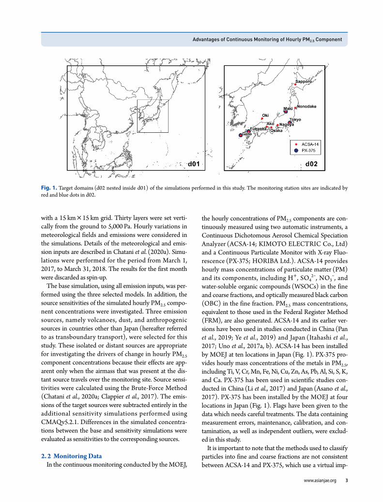
Figure 1 shows the target study domains, with d02 nested inside d01. These domains are commonly used in model comparisons in Japan’s Study for Reference Air Quality Modeling ( J­STREAM) project (Chatani et al., 2018). The larger domain (d01) covers Asian countries with a 45 km × 45 km grid and provides boundary con­centrations for d02. The boundary concentrations for d01 were derived from the chemical atmospheric general circulation model for the study of the atmospheric envi­ronment and radiative forcing (CHASER) (Sudo et al., 2002). The nested domain (d02) covers most of Japan

Advantages of Continuous Monitoring of Hourly PM2.5 Component

www.asianjae.org 3

with a 15 km × 15 km grid. Thirty layers were set verti­cally from the ground to 5,000 Pa. Hourly variations in meteorological fields and emissions were considered in the simulations. Details of the meteorological and emis­sion inputs are described in Chatani et al. (2020a). Simu­lations were performed for the period from March 1, 2017, to March 31, 2018. The results for the first month were discarded as spin­up.

The base simulation, using all emission inputs, was per­formed using the three selected models. In addition, the source sensitivities of the simulated hourly PM2.5 compo­nent concentrations were investigated. Three emission sources, namely volcanoes, dust, and anthropogenic sources in countries other than Japan (hereafter referred to as transboundary transport), were selected for this study. These isolated or distant sources are appropriate for investigating the drivers of change in hourly PM2.5 component concentrations because their effects are app­arent only when the airmass that was present at the dis­tant source travels over the monitoring site. Source sensi­tivities were calculated using the Brute­Force Method

(Chatani et al., 2020a; Clappier et al., 2017). The emis­sions of the target sources were subtracted entirely in the additional sensitivity simulations performed using CMAQv5.2.1. Differences in the simulated concentra­tions between the base and sensitivity simulations were evaluated as sensitivities to the corresponding sources.

2. 2 Monitoring DataIn the continuous monitoring conducted by the MOEJ,

the hourly concentrations of PM2.5 components are con­tinuously measured using two automatic instruments, a Continuous Dichotomous Aerosol Chemical Speciation Analyzer (ACSA­14; KIMOTO ELECTRIC Co., Ltd) and a Continuous Particulate Monitor with X­ray Fluo­rescence (PX­375; HORIBA Ltd.). ACSA­14 provides hourly mass concentrations of particulate matter (PM) and its components, including H+, SO4

2-, NO3-, and

water­soluble organic compounds (WSOCs) in the fine and coarse fractions, and optically measured black carbon

(OBC) in the fine fraction. PM2.5 mass concentrations, equivalent to those used in the Federal Register Method

(FRM), are also generated. ACSA­14 and its earlier ver­sions have been used in studies conducted in China (Pan et al., 2019; Ye et al., 2019) and Japan (Itahashi et al., 2017; Uno et al., 2017a, b). ACSA­14 has been installed by MOEJ at ten locations in Japan (Fig. 1). PX­375 pro­vides hourly mass concentrations of the metals in PM2.5, including Ti, V, Cr, Mn, Fe, Ni, Cu, Zn, As, Pb, Al, Si, S, K, and Ca. PX­375 has been used in scientific studies con­ducted in China (Li et al., 2017) and Japan (Asano et al., 2017). PX­375 has been installed by the MOEJ at four locations in Japan (Fig. 1). Flags have been given to the data which needs careful treatments. The data containing measurement errors, maintenance, calibration, and con­tamination, as well as independent outliers, were exclud­ed in this study.

It is important to note that the methods used to classify particles into fine and coarse fractions are not consistent between ACSA­14 and PX­375, which use a virtual imp­

Fig. 1. Target domains (d02 nested inside d01) of the simulations performed in this study. The monitoring station sites are indicated by red and blue dots in d02.

Asian Journal of Atmospheric Environment, Vol. 15, No. 2, 2021008, 2021

4 www.asianjae.org

actor and a FRM impactor, respectively. Although both are intended to classify PM2.5, Nakatsubo et al. (2018) reported differences between the PM2.5 mass concentra­tions classified by ACSA­14 and FRM. Further, the meth­ods used to represent particle size distributions are not consistent between CMAQ and CAMx. CMAQ uses three modal size distributions and PM2.5 is represented by the Aitken and accumulation modes (Binkowski and Ros­elle, 2003). CAMx uses two discrete bins for coarse and fine particles, and the latter represents PM2.5. These dif­ferent treatments and particle evolution may result in dif­ferences in PM2.5 concentrations simulated by them. It is difficult to maintain strict particle size consistency among the observed and simulated values. We compared the simulated values of the Aitken and accumulation modes of CMAQ and the “fine” bin of CAMx, with the observed PX­375 and ACSA­14 (fine fraction) values. CMAQ­sim­ulated values of the coarse mode were compared with the

observed ACSA­14 coarse­fraction values. Although using inconsistent size classifications might result in data gaps, our discussion focused mainly on the correlation between the observed and simulated concentrations.

3. RESULTS AND DISCUSSION

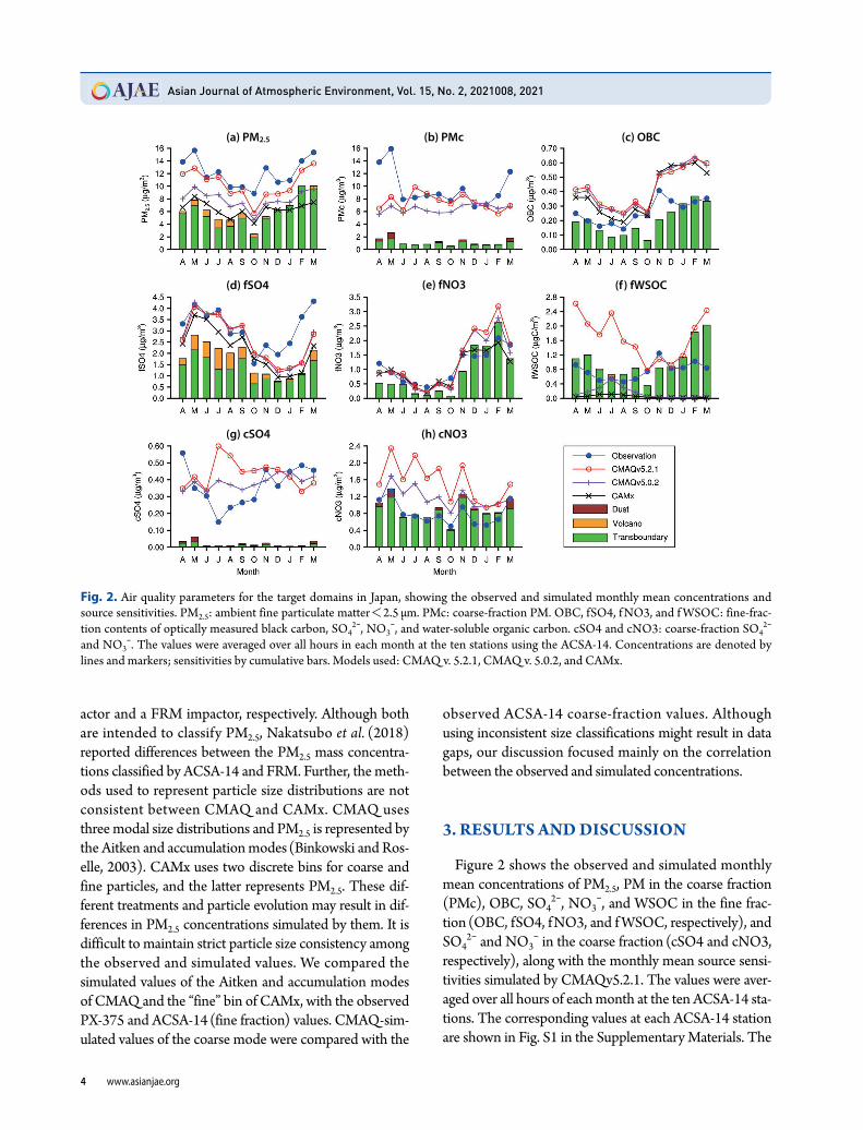
Figure 2 shows the observed and simulated monthly mean concentrations of PM2.5, PM in the coarse fraction

(PMc), OBC, SO42-, NO3

-, and WSOC in the fine frac­tion (OBC, fSO4, fNO3, and f WSOC, respectively), and SO4

2- and NO3- in the coarse fraction (cSO4 and cNO3,

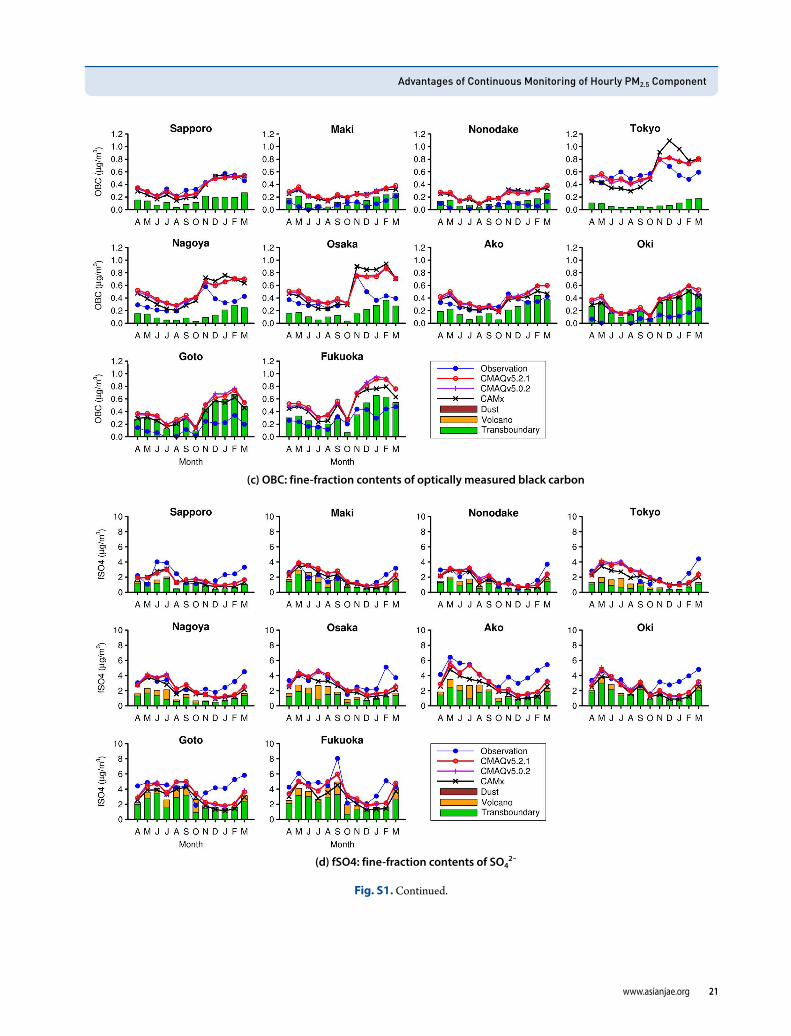
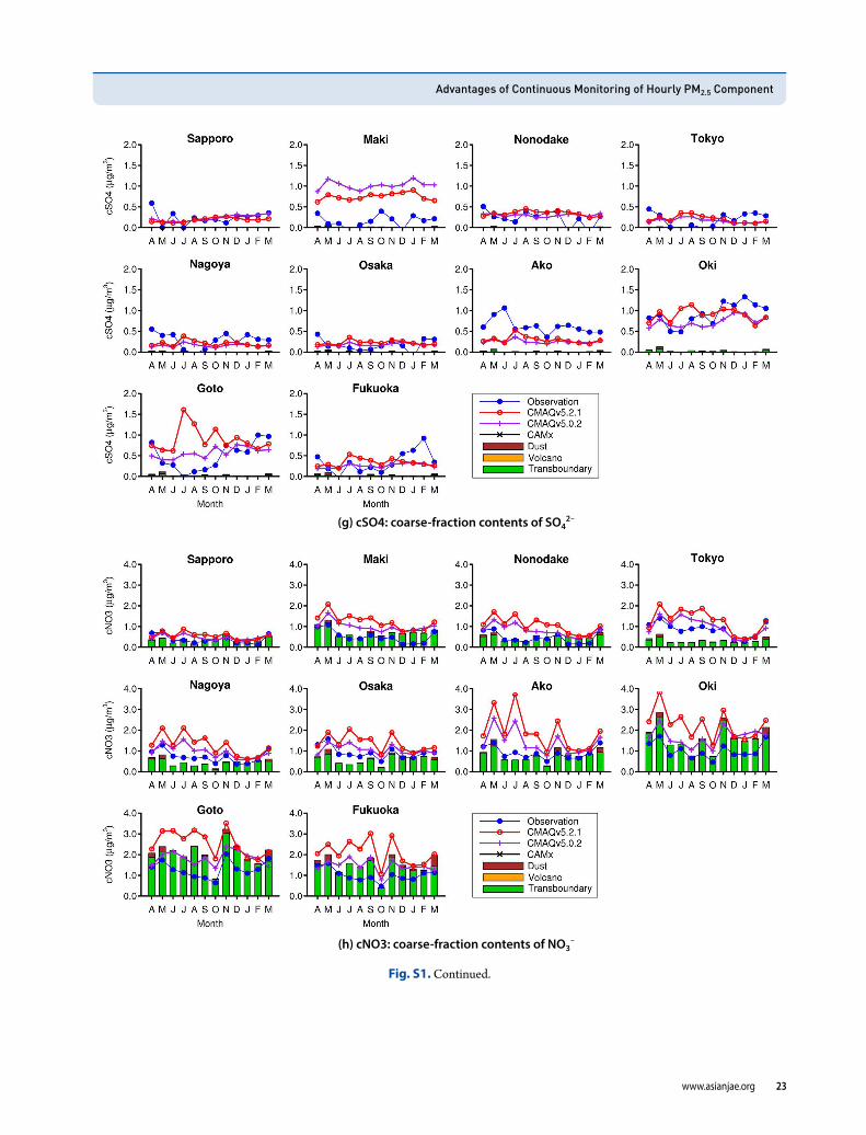
respectively), along with the monthly mean source sensi­tivities simulated by CMAQv5.2.1. The values were aver­aged over all hours of each month at the ten ACSA­14 sta­tions. The corresponding values at each ACSA­14 station are shown in Fig. S1 in the Supplementary Materials. The

(a) PM2.5

(d) fSO4

(g) cSO4

(e) fNO3 (f) fWSOC

(h) cNO3

(b) PMc (c) OBC

Fig. 2. Air quality parameters for the target domains in Japan, showing the observed and simulated monthly mean concentrations and source sensitivities. PM2.5: ambient fine particulate matter<2.5 μm. PMc: coarse­fraction PM. OBC, fSO4, f NO3, and f WSOC: fine­frac­tion contents of optically measured black carbon, SO4

2-, NO3-, and water­soluble organic carbon. cSO4 and cNO3: coarse­fraction SO4

2- and NO3

-. The values were averaged over all hours in each month at the ten stations using the ACSA­14. Concentrations are denoted by lines and markers; sensitivities by cumulative bars. Models used: CMAQ v. 5.2.1, CMAQ v. 5.0.2, and CAMx.

Advantages of Continuous Monitoring of Hourly PM2.5 Component

www.asianjae.org 5

simulated concentrations of elemental carbon (EC) were compared with the observed OBC concentrations. WSOC is a marker of secondary organic aerosols (SOAs)

(Kondo et al., 2007; Miyazaki et al., 2006). The simulated concentrations of secondary organic carbon (SOC) were compared with the observed WSOC concentrations.

Distinct seasonal variations in PM2.5 concentrations were observed (Fig. 2a), with higher concentrations in the spring and lower concentrations in the summer and early autumn. Although these seasonal variations were repro­duced well by the models, the absolute values were under ­ estimated. Among the three models, the CMAQv5.2.1­simulated values were the closest to the observed value. The underestimation was more evident in eastern Japan, as indicated by Chatani et al. (2020a). The PM2.5 concen­trations simulated by CMAQv5.2.1 were higher than the observed values at Fukuoka, which is located in western Japan (Fig. S1a). The simulated sensitivity to transboun­dary transport corresponded to 30­80% of the simulated PM2.5 concentrations.

The models performed well in terms of simulating PMc

concentrations, except in the spring, during which higher peaks were observed (Fig. 2b). The simulated sensitivities of PMc concentrations to volcanic emissions, dust, and transboundary transport were relatively small. The influ­ence of other emission sources, including sea salt, seemed to be larger, given that Na and Cl were the most influen­tial components in the simulated PMc concentrations

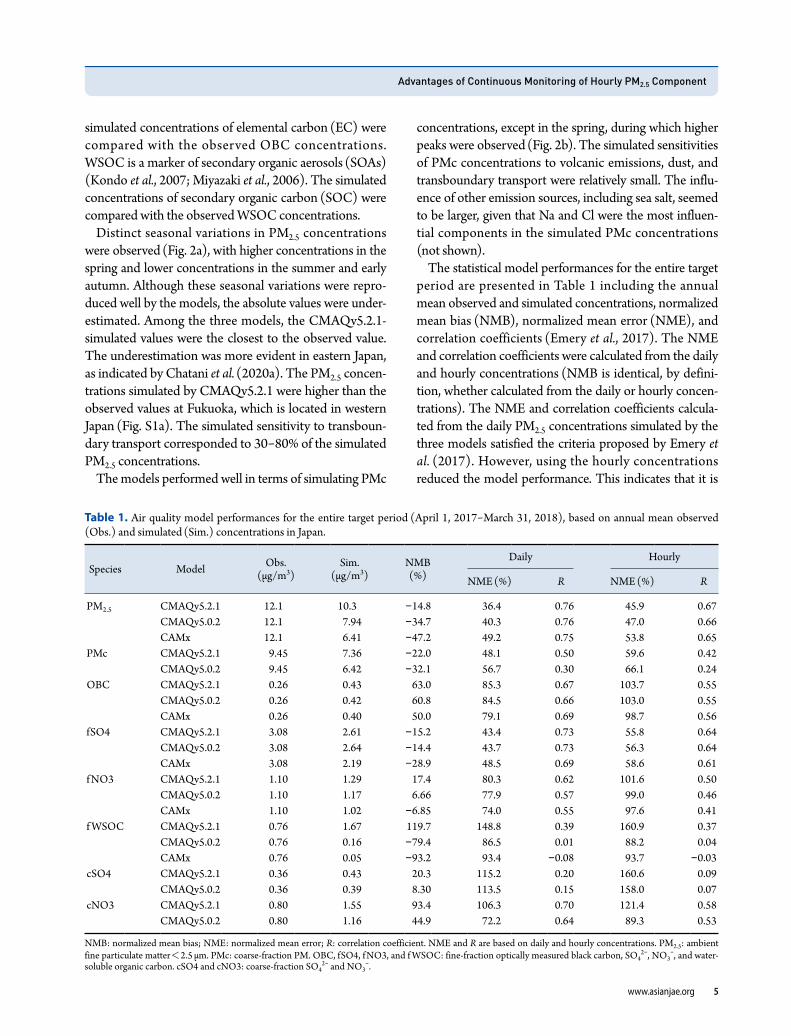
(not shown).The statistical model performances for the entire target

period are presented in Table 1 including the annual mean observed and simulated concentrations, normalized mean bias (NMB), normalized mean error (NME), and cor rela tion coefficients (Emery et al., 2017). The NME and correlation coefficients were calculated from the daily and hourly concentrations (NMB is identical, by defini­tion, whether calculated from the daily or hourly concen­trations). The NME and correlation coefficients calcula­ted from the daily PM2.5 concentrations simulated by the three models satisfied the criteria proposed by Emery et al. (2017). However, using the hourly concentrations reduced the model performance. This indicates that it is

Table 1. Air quality model performances for the entire target period (April 1, 2017­March 31, 2018), based on annual mean observed

(Obs.) and simulated (Sim.) concentrations in Japan.

Species Model Obs.(μg/m3)

Sim.(μg/m3)

NMB(%)

Daily Hourly

NME (%) R NME (%) R

PM2.5 CMAQv5.2.1 12.1 10.3 -14.8 36.4 0.76 45.9 0.67CMAQv5.0.2 12.1 7.94 -34.7 40.3 0.76 47.0 0.66CAMx 12.1 6.41 -47.2 49.2 0.75 53.8 0.65

PMc CMAQv5.2.1 9.45 7.36 -22.0 48.1 0.50 59.6 0.42CMAQv5.0.2 9.45 6.42 -32.1 56.7 0.30 66.1 0.24

OBC CMAQv5.2.1 0.26 0.43 63.0 85.3 0.67 103.7 0.55CMAQv5.0.2 0.26 0.42 60.8 84.5 0.66 103.0 0.55CAMx 0.26 0.40 50.0 79.1 0.69 98.7 0.56

fSO4 CMAQv5.2.1 3.08 2.61 -15.2 43.4 0.73 55.8 0.64CMAQv5.0.2 3.08 2.64 -14.4 43.7 0.73 56.3 0.64CAMx 3.08 2.19 -28.9 48.5 0.69 58.6 0.61

f NO3 CMAQv5.2.1 1.10 1.29 17.4 80.3 0.62 101.6 0.50CMAQv5.0.2 1.10 1.17 6.66 77.9 0.57 99.0 0.46CAMx 1.10 1.02 -6.85 74.0 0.55 97.6 0.41

f WSOC CMAQv5.2.1 0.76 1.67 119.7 148.8 0.39 160.9 0.37CMAQv5.0.2 0.76 0.16 -79.4 86.5 0.01 88.2 0.04CAMx 0.76 0.05 -93.2 93.4 -0.08 93.7 -0.03

cSO4 CMAQv5.2.1 0.36 0.43 20.3 115.2 0.20 160.6 0.09CMAQv5.0.2 0.36 0.39 8.30 113.5 0.15 158.0 0.07

cNO3 CMAQv5.2.1 0.80 1.55 93.4 106.3 0.70 121.4 0.58CMAQv5.0.2 0.80 1.16 44.9 72.2 0.64 89.3 0.53

NMB: normalized mean bias; NME: normalized mean error; R: correlation coefficient. NME and R are based on daily and hourly concentrations. PM2.5: ambient fine particulate matter<2.5 µm. PMc: coarse­fraction PM. OBC, fSO4, f NO3, and f WSOC: fine­fraction optically measured black carbon, SO4

2-, NO3-, and water­

soluble organic carbon. cSO4 and cNO3: coarse­fraction SO42- and NO3

-.

Asian Journal of Atmospheric Environment, Vol. 15, No. 2, 2021008, 2021

6 www.asianjae.org

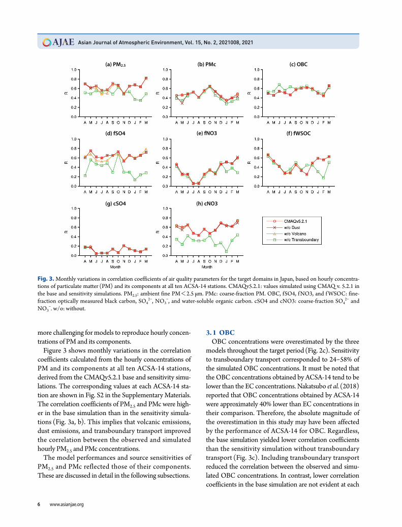
more challenging for models to reproduce hourly concen­trations of PM and its components.

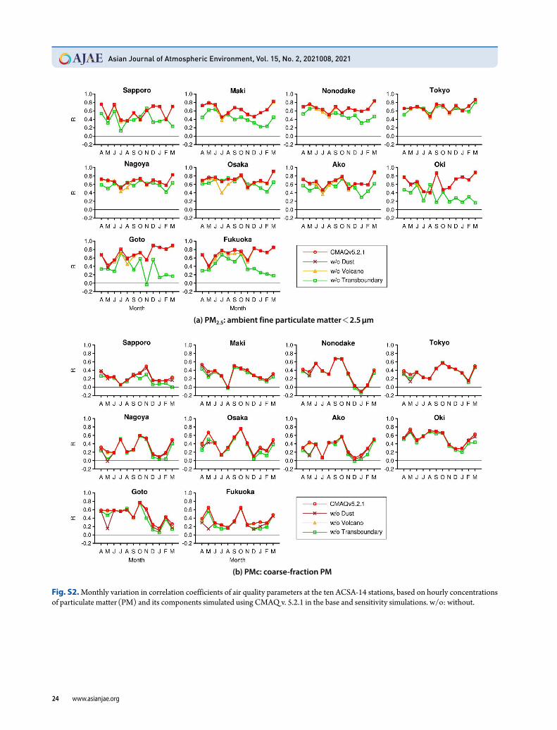
Figure 3 shows monthly variations in the correlation coefficients calculated from the hourly concentrations of PM and its components at all ten ACSA­14 stations, derived from the CMAQv5.2.1 base and sensitivity simu­lations. The corresponding values at each ACSA­14 sta­tion are shown in Fig. S2 in the Supplementary Materials. The correlation coefficients of PM2.5 and PMc were high­er in the base simulation than in the sensitivity simula­tions (Fig. 3a, b). This implies that volcanic emissions, dust emissions, and transboundary transport improved the correlation between the observed and simulated hourly PM2.5 and PMc concentrations.

The model performances and source sensitivities of PM2.5 and PMc reflected those of their components. These are discussed in detail in the following subsections.

3. 1 OBCOBC concentrations were overestimated by the three

models throughout the target period (Fig. 2c). Sensitivity to transboundary transport corresponded to 24­58% of the simulated OBC concentrations. It must be noted that the OBC concentrations obtained by ACSA­14 tend to be lower than the EC concentrations. Nakatsubo et al. (2018) reported that OBC concentrations obtained by ACSA­14 were approximately 40% lower than EC concentrations in their comparison. Therefore, the absolute magnitude of the overestimation in this study may have been affected by the performance of ACSA­14 for OBC. Regardless, the base simulation yielded lower correlation coefficients than the sensitivity simulation without transboundary transport (Fig. 3c). Including transboundary trans port reduced the correlation between the observed and simu­lated OBC concentrations. In contrast, lower correlation coeffic ients in the base simulation are not evident at each

(a) PM2.5

(d) fSO4

(g) cSO4

(e) fNO3 (f) fWSOC

Fig. 3. Monthly variations in correlation coefficients of air quality parameters for the target domains in Japan, based on hourly concentra­tions of particulate matter (PM) and its components at all ten ACSA­14 stations. CMAQv5.2.1: values simulated using CMAQ v. 5.2.1 in the base and sensitivity simulations. PM2.5: ambient fine PM<2.5 μm. PMc: coarse­fraction PM. OBC, fSO4, f NO3, and f WSOC: fine­fraction optically measured black carbon, SO4

2-, NO3-, and water­soluble organic carbon. cSO4 and cNO3: coarse­fraction SO4

2- and NO3

-. w/o: without.

(h) cNO3

(b) PMc (c) OBC

Advantages of Continuous Monitoring of Hourly PM2.5 Component

www.asianjae.org 7

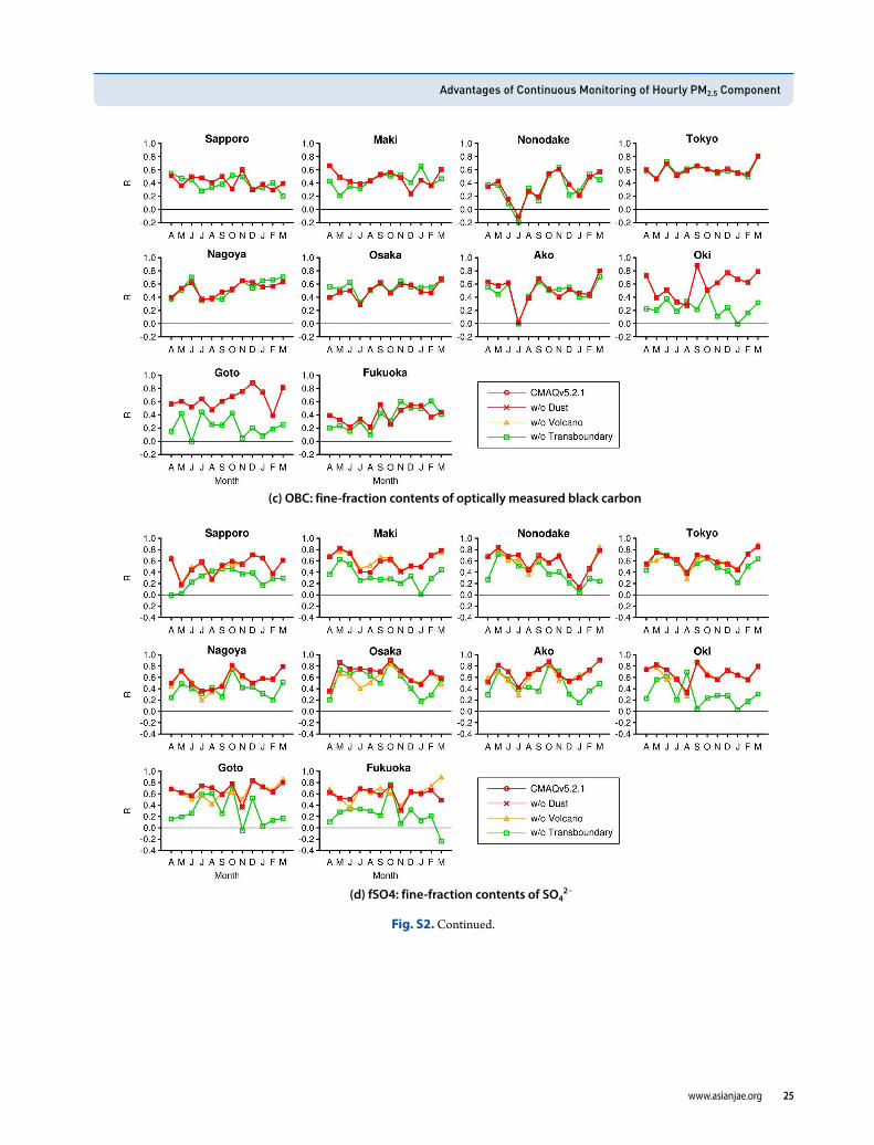
station(Fig. S2c). Thus, the inclusion of trans boundary transport redu ced the spatial correlations among the ten ACSA­14 stations, whereas it contributed to better tempo­ral correlations, particularly at stations located in remote areas of western Japan such as Oki and Goto. As shown in Fig. S1c, the base simulation had a better performance at the stations located in urban areas, including Sapporo, Tokyo, Nagoya, and Osaka. Overestimation mainly occu r­red in remote areas when influences of transboundary transport were large. The inclusion of transboundary trans­port resulted in spatial inconsistencies in model perfor­mance between urban and remote areas.

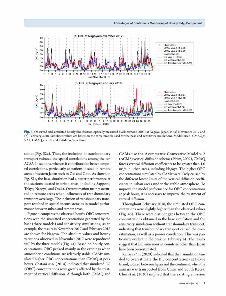
Figure 4 compares the observed hourly OBC concentra­tions with the simulated concentrations generated by the base (three models) and sensitivity simulations; as an example, the results in November 2017 and February 2018 are shown for Nagoya. The absolute values and hourly variations observed in November 2017 were reproduced well by the three models (Fig. 4a). Based on hourly con­centrations, OBC peaked mainly in the evenings when atmospheric conditions are relatively stable. CAMx sim­ulated higher OBC concentrations than CMAQ at peak hours. Chatani et al. (2014) indicated that simulated EC

(OBC) concentrations were greatly affected by the treat­ment of vertical diffusion. Although both CMAQ and

CAMx use the Asymmetric Convective Model v. 2

(ACM2) vertical diffusion scheme (Pleim, 2007), CMAQ forces vertical diffusion coefficients to be greater than 1.0

m2/s in urban areas, including Nagoya. The higher OBC concentrations simulated by CAMx were likely caused by the different lower limits of the vertical diffusion coeffi­cients in urban areas under the stable atmosphere. To improve the model performance for OBC concentrations at peak hours, it is necessary to improve the treatment of vertical diffusion.

Throughout February 2018, the simulated OBC con­centrations were slightly higher than the observed values

(Fig. 4b). There were distinct gaps between the OBC concentrations obtained in the base simulation and the sensitivity simulation without transboundary transport, indicating that transboundary transport caused the over­estimation, as well as a poorer correlation. This was par­ticularly evident in the peak on February 24. The results suggest that BC emissions in countries other than Japan have been overestimated.

Kanaya et al. (2020) indicated that their simulation ten­ded to overestimate the BC concentrations at Fukue Island, located between Japan and the continent, when the airmass was transported from China and South Korea. Choi et al. (2020) implied that the existing emission

(a) OBC at Nagoya (November 2017)

(b) OBC at Nagoya (February 2018)

Fig. 4. Observed and simulated hourly fine­fraction optically measured black carbon (OBC) at Nagoya, Japan, in (a) November 2017 and (b) February 2018. Simulated values are based on the three models used for the base and sensitivity simulations. Models used: CMAQ v. 5.2.1, CMAQ v. 5.0.2, and CAMx. w/o: without.

Asian Journal of Atmospheric Environment, Vol. 15, No. 2, 2021008, 2021

8 www.asianjae.org

inventories, including the Hemispheric Transport of Air Pollution (HTAP) emissions v. 2.2 ( Janssens­Maenhout et al., 2015), used in this study, overestimated the BC/CO ratios of the emissions in China and South Korea. The results obtained in this study were consistent with their findings. However, it must also be noted that Febru­ary 2018, which had larger discrepancies between the obser ved and simulated OBC concentrations (Fig. 2c), had the lowest correlation coefficients (0.48), even in the sensiti vity simulation without transboundary transport

(Fig. 3c). Both the decrease in OBC originating from transboundary transport and the increase in OBC origi­nating from local emissions are expected to improve spa­tial correlations.

3. 2 SO42-

The statistical model performance for fSO4 was com­parable to that for PM2.5

(Table 1), satisfying the criteria proposed by Emery et al. (2017). The observed fSO4 concentrations were higher during the first half of the tar­get period (spring and summer; Fig. 2d). Their absolute values and monthly variations were reproduced well by the three models. In contrast, during the second half of the target period (autumn and winter), these values were underestimated by the three models. Previous studies

(Itahashi et al., 2018b; Morino et al., 2015) also reported the underestimation of winter SO4

2- concentrations around Japan. The models may need to be updated by including additional aqueous­ and gaseous­phase oxida­tion pathways, to improve their performances for winter SO4

2- values (Itahashi et al., 2019, 2018a). Itahashi et al.

(2018b) indicated that differences between CAMx and CMAQv5.0.2 regarding how dry deposition is represen­ted resulted in CAMx simulating higher SO4

2- concen­trations. The opposite pattern that we obtained in this study may be due to another difference: we used CMAQ v5.0.2 calculating photolysis rates online, whereas CAMx picked them up from a lookup table. Differences in pho­tolysis rates could affect the secondary formation of rele­vant species in the atmosphere, including SO4

2- (Chatani et al., 2020b; Itahashi et al., 2020b).

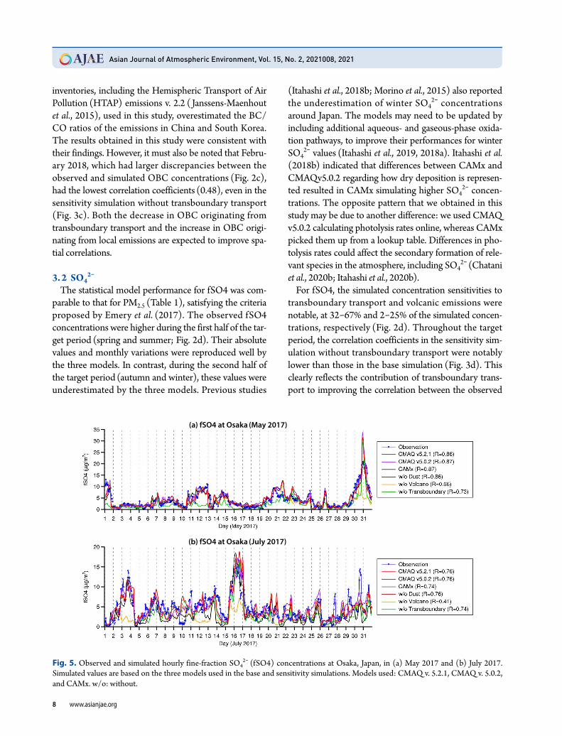
For fSO4, the simulated concentration sensitivities to transboundary transport and volcanic emissions were notable, at 32­67% and 2­25% of the simulated concen­trations, respectively (Fig. 2d). Throughout the target period, the correlation coefficients in the sensitivity sim­ulation without transboundary transport were notably lower than those in the base simulation (Fig. 3d). This clearly reflects the contribution of transboundary trans­port to improving the correlation between the observed

(a) fSO4 at Osaka (May 2017)

(b) fSO4 at Osaka (July 2017)

Fig. 5. Observed and simulated hourly fine­fraction SO42- (fSO4) concentrations at Osaka, Japan, in (a) May 2017 and (b) July 2017.

Simulated values are based on the three models used in the base and sensitivity simulations. Models used: CMAQ v. 5.2.1, CMAQ v. 5.0.2, and CAMx. w/o: without.

Advantages of Continuous Monitoring of Hourly PM2.5 Component

www.asianjae.org 9

and simulated fSO4 concentrations. The contribution of volcanic emissions was also evident from May to August.

Figure 5 compares the observed hourly fSO4 concen­trations with the simulated concentrations derived from the base (three models) and sensitivity simulations, using Osaka in May and July 2017 as an example. Hourly varia­tions in observed fSO4 concentrations were reproduced well by the three models. The fSO4 concentrations simu­lated in the sensitivity simulation without transboundary transport had distinctly lower peaks than those simul ­ ated in the base simulation on May 1, 12, 20, and 30 (Fig. 5a), clearly illustrating the influence of transboundary transport on these days. Likewise, the fSO4 concentra­tions simulated in the sensitivity simulation without vol­canic emissions had distinctly lower peaks on July 3, 12, and 16 (Fig. 5b), clearly illustrating influence of volcanic emissions on these days.

In contrast, the models performed worse in simulating cSO4 concentrations (Table 1). While the observed and simulated annual cSO4 concentrations were comparable, the NME was large and the correlation coefficients were quite low (Fig. 3g). The simulated sensitivities of cSO4 concentrations to the three emission sources were small

(Fig. 2g). This implies that the factors affecting cSO4 were entirely different from those affecting fSO4. Osada et al. (2016) reported low correlations between cSO4 con­cen trations measured using the ACSA and those mea su­red by collection on filters. These findings suggest that there are large uncertainties in both the observed and sim ­ ulated cSO4 concentrations.

3. 3 NO3

-

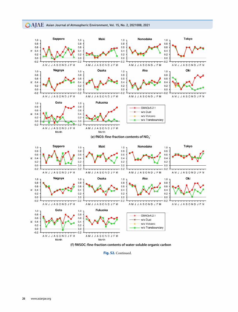
There were distinct seasonal variations in the f NO3 concentration (Fig. 2e). Observed f NO3 concentrations were much higher during the winter than the summer. This seasonal variation was reproduced well by the mod­els. However, the higher winter f NO3 concentrations were overestimated by the CMAQ models, particularly in western Japan, including Oki, Goto, and Fukuoka (Fig. S1e). Most of the overestimation was due to transboun­dary transport, even though it improved the correlation during the winter (Fig. 3e and Fig. S2e). The overestima­tion of summer NO3

- concentrations, which has been previously reported (Shimadera et al., 2014), was not evi­dent in this study. The observed cNO3 concentrations did not exhibit distinct seasonal variations (Fig. 2h). In contrast to fNO3, the models overestimated cNO3 thro­u ghout the target period. Transboundary transport imp­

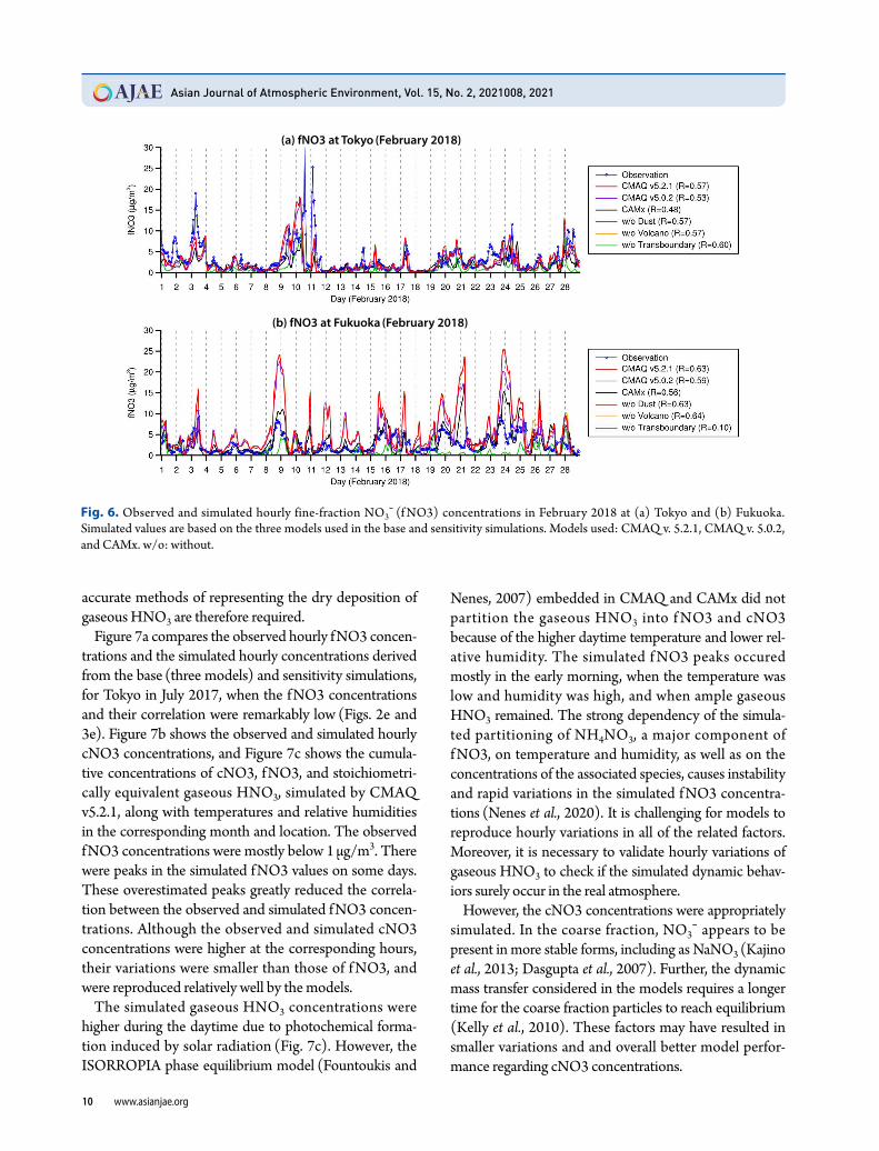
roved the cNO3 correlations (Fig. 3h).Figure 6 compares the observed hourly fNO3 concen­

trations with the simulated concentrations derived from the base (three models) and sensitivity simulations, using February 2018 in Tokyo (eastern Japan) and Fukuoka

(wes tern Japan), as examples. At Tokyo, while the obser­ved f NO3 concentrations were relatively low on most days, there were peaks on some days (Fig. 6a). The models did not satisfactorily reproduce some of these peaks

(those on February 3 and 11). Itahashi et al. (2020b) con ­ ducted a detailed analysis of the model performance for winter NO3

- concentrations in Tokyo, finding that NOX and NH3 emissions, heterogeneous reactions involving HONO, and photolysis rates were critical factors that affect model performance in terms of simulating NO3

- concentration peaks. Unlike Tokyo, at Fukuoka (western Japan) many of the peaks were higher, albeit flatter, and all were significantly overestimated by the CMAQ models

(Fig. 6b). The fNO3 concentrations and correlation coef­ficients based on the sensitivity simulation without trans­boundary transport were substantially lower than those in the base simulation, indicating that they were exclusively and excessively affected by transboundary transport. Uno et al. (2020) indicated that the recent reduction in SOX emissions realized by the stringent emission controls imp­l e mented in China caused a paradigm shift and inc reased NO3

- transport to western Japan, particularly during colder seasons (Itahashi et al., 2017). Although their find­ings are related to our simulated results, the influence of transboundary transport on the fNO3 concentration was too large. As mentioned, the winter fSO4 concentrations were underestimated by the models used in this study. When more fSO4 is available, the simulated fNO3 con­cen trations should decrease, according to the paradigm discussed by Uno et al. (2020). The possible impacts of imp roved model performance on winter fSO4 concen­trations (discussed in section 3.2), are also important for addressing the problem of overestimated fNO3 concen­trations. Further, the CAMx­simulated peak values were substantially lower than those simulated by CMAQ. It is known that the inaccurate estimation of gaseous HNO3 dry deposition velocity can cause the overestimation of NO3

- concentrations (Itahashi et al., 2017; Morino et al., 2015; Shimadera et al., 2014). CMAQ and CAMx use different dry deposition schemes, M3DRY (Otte and Pleim, 2010) and that of Zhang et al. (2003), respective­ly, which might have caused the differences in the fNO3 concentrations simulated by CMAQ and CAMx. More

Asian Journal of Atmospheric Environment, Vol. 15, No. 2, 2021008, 2021

10 www.asianjae.org

accurate methods of representing the dry deposition of gaseous HNO3 are therefore required.

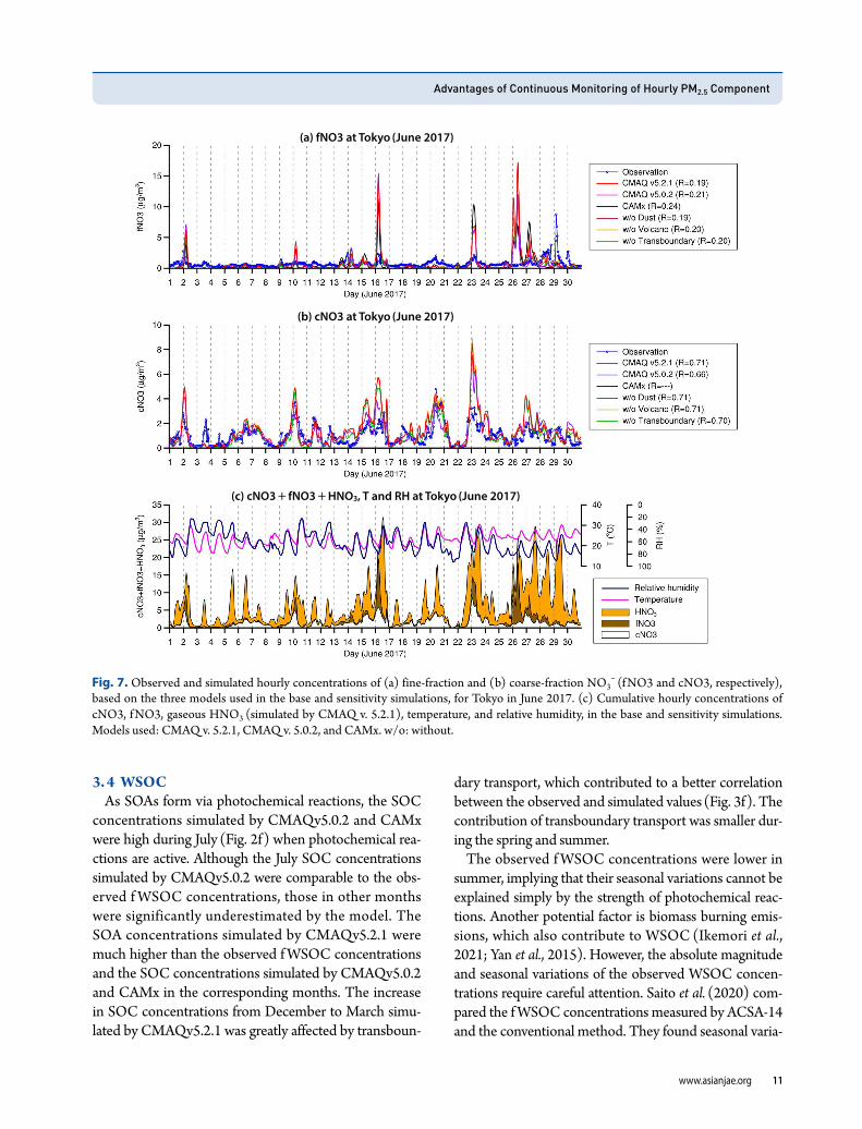
Figure 7a compares the observed hourly fNO3 concen ­ trations and the simulated hourly concentrations derived from the base (three models) and sensitivity simulations, for Tokyo in July 2017, when the f NO3 concentrations and their correlation were remarkably low (Figs. 2e and 3e). Figure 7b shows the observed and simulated hourly cNO3 concentrations, and Figure 7c shows the cumula­tive concentrations of cNO3, fNO3, and stoichiometri­cally equivalent gaseous HNO3, simulated by CMAQ v5.2.1, along with temperatures and relative humidities in the corresponding month and location. The observed fNO3 concentrations were mostly below 1 μg/m3. There were peaks in the simulated fNO3 values on some days. These overestimated peaks greatly reduced the correla­tion between the observed and simulated fNO3 concen­trations. Although the observed and simulated cNO3 con centrations were higher at the corresponding hours, their variations were smaller than those of f NO3, and were reproduced relatively well by the models.

The simulated gaseous HNO3 concentrations were higher during the daytime due to photochemical forma­tion induced by solar radiation (Fig. 7c). However, the ISORROPIA phase equilibrium model (Fountoukis and

Nenes, 2007) embedded in CMAQ and CAMx did not par tition the gaseous HNO3 into f NO3 and cNO3 becau se of the higher daytime temperature and lower rel­a tive humidity. The simulated f NO3 peaks occured mostly in the early morning, when the temperature was low and humidity was high, and when ample gaseous HNO3 remained. The strong dependency of the simula­ted partitioning of NH4NO3, a major component of f NO3, on temperature and humidity, as well as on the concentrations of the associated species, causes instability and rapid variations in the simulated f NO3 concentra­tions (Nenes et al., 2020). It is challenging for models to reproduce hourly variations in all of the related factors. Moreover, it is necessary to validate hourly variations of gaseous HNO3 to check if the simulated dynamic behav­iors surely occur in the real atmosphere.

However, the cNO3 concentrations were appropriately simulated. In the coarse fraction, NO3

- appears to be present in more stable forms, including as NaNO3

(Kajino et al., 2013; Dasgupta et al., 2007). Further, the dynamic mass transfer considered in the models requires a longer time for the coarse fraction particles to reach equilibrium

(Kelly et al., 2010). These factors may have resulted in smaller variations and and overall better model perfor­mance regarding cNO3 concentrations.

(a) fNO3 at Tokyo (February 2018)

(b) fNO3 at Fukuoka (February 2018)

Fig. 6. Observed and simulated hourly fine­fraction NO3- (f NO3) concentrations in February 2018 at (a) Tokyo and (b) Fukuoka.

Simulated values are based on the three models used in the base and sensitivity simulations. Models used: CMAQ v. 5.2.1, CMAQ v. 5.0.2, and CAMx. w/o: without.

Advantages of Continuous Monitoring of Hourly PM2.5 Component

www.asianjae.org 11

3. 4 WSOCAs SOAs form via photochemical reactions, the SOC

concentrations simulated by CMAQv5.0.2 and CAMx were high during July (Fig. 2f) when photochemical rea­c tions are active. Although the July SOC concentrations simulated by CMAQv5.0.2 were comparable to the obs­erved f WSOC concentrations, those in other months were significantly underestimated by the model. The SOA concentrations simulated by CMAQv5.2.1 were much higher than the observed f WSOC concentrations and the SOC concentrations simulated by CMAQv5.0.2 and CAMx in the corresponding months. The increase in SOC concentrations from December to March simu­lated by CMAQv5.2.1 was greatly affected by transboun­

dary transport, which contributed to a better correlation between the observed and simulated values (Fig. 3f). The contribution of transboundary transport was smaller dur­ing the spring and summer.

The observed f WSOC concentrations were lower in summer, implying that their seasonal variations cannot be explained simply by the strength of photochemical reac­tions. Another potential factor is biomass burning emis­sions, which also contribute to WSOC (Ikemori et al., 2021; Yan et al., 2015). However, the absolute magnitude and seasonal variations of the observed WSOC concen­trations require careful attention. Saito et al. (2020) com­pared the f WSOC concentrations measured by ACSA­14 and the conventional method. They found seasonal varia­

(a) fNO3 at Tokyo (June 2017)

(b) cNO3 at Tokyo (June 2017)

Fig. 7. Observed and simulated hourly concentrations of (a) fine­fraction and (b) coarse­fraction NO3- (f NO3 and cNO3, respectively),

based on the three models used in the base and sensitivity simulations, for Tokyo in June 2017. (c) Cumulative hourly concentrations of cNO3, f NO3, gaseous HNO3

(simulated by CMAQ v. 5.2.1), temperature, and relative humidity, in the base and sensitivity simulations. Models used: CMAQ v. 5.2.1, CMAQ v. 5.0.2, and CAMx. w/o: without.

(c) cNO3 + fNO3 + HNO3, T and RH at Tokyo (June 2017)

Asian Journal of Atmospheric Environment, Vol. 15, No. 2, 2021008, 2021

12 www.asianjae.org

tions in the slopes and intercepts of the regression lines between them. The discrepancies were larger in the sum­mer than the winter, possibly caused by seasonal varia­tions in the WSOC compositions. In addition, compo­nents including levoglucosan, which is a well known marker for biomass burning emissions, cannot be detected by ACSA­14 using ultraviolet spectrophotometry. Addi­tional research is necessary to clarify the relationships among f WSOC concentrations measured by ACSA­14 and by the conventional method, as well as SOA concen­trations simulated by the models.

CMAQ v. 5.2 and later versions have incorporated par­titioning and aging of semi­volatile organic aerosols

(Robinson et al., 2007; Donahue et al., 2006). Along with this treatment, they have introduced a new surrogate spe­cies, which is a potential SOA from combustion emis­sions (pcSOA). pcSOA represents the SOA that was missed in the preceding models for various reasons, including SOA formation from intermediate­volatility organic compound (IVOC) emissions, which are not included in current emission inventories (Murphy et al., 2017). In CMAQv5.2.1, an amount equivalent to 6.6 times the primary organic aerosol (POA) emissions is ingested as missing emissions of pcVOC (precursors of pcSOA), which are subsequently oxidized in the atmo­

sphere to form pcSOA. In our simulations, pcSOA occu­pied a large fraction of the simulated SOC concentra­tions (not shown), leading to overestimation and differ­ences in seasonal variations of the simulated SOC con­centrations (Fig. 2f).

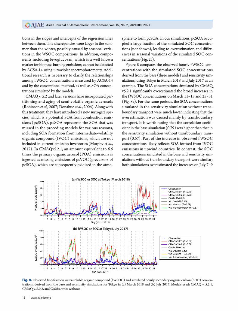
Figure 8 compares the observed hourly f WSOC con­centrations with the simulated SOC concentrations derived from the base (three models) and sensitivity sim­ulations, using Tokyo in March 2018 and July 2017 as an example. The SOA concentrations simulated by CMAQ v5.2.1 significantly overestimated the broad increases in the f WSOC concentrations on March 11­15 and 25­31

(Fig. 8a). For the same periods, the SOA concentrations simulated in the sensitivity simulation without trans­boundary transport were much lower, indicating that the overestimation was caused mainly by transboundary transport. It is worth noting that the correlation coeffi­cient in the base simulation (0.79) was higher than that in the sensitivity simulation without transboundary trans ­ port (0.67). Part of the increase in observed f WSOC concentrations likely reflects SOA formed from IVOC emissions in upwind countries. In contrast, the SOC concentrations simulated in the base and sensitivity sim­ulations without transboundary transport were similar; both simulations overestimated the increases on July 7­9

(a) fWSOC or SOC at Tokyo (March 2018)

(b) fWSOC or SOC at Tokyo (July 2017)

Fig. 8. Observed fine­fraction water­soluble organic compound (f WSOC) and simulated hourly secondary organic carbon (SOC) concen­trations, derived from the base and sensitivity simulations for Tokyo in (a) March 2018 and (b) July 2017. Models used: CMAQ v. 5.2.1, CMAQ v. 5.0.2, and CAMx. w/o: without.

Advantages of Continuous Monitoring of Hourly PM2.5 Component

www.asianjae.org 13

and 16­20 (Fig. 8b). The SOC concentrations simulated by CMAQv5.0.2 were closer to the observed values in the corresponding period. The later versions of CMAQ did not perform well for modeling summer pcSOA formed from IVOC emissions in Japan.

The emission ratio of pcVOC to POA is an uncertain parameter in the treatment incorporated in CMAQv5.2.1

(Murphy et al., 2017). While its value (6.6) has been vali­dated in comparisons with observations conducted in the United States, this value may not be suitable for Asia, where POA emissions are relatively high because there are fewer emission controls. Suitable values for the pcVOC/ POA ratio need to be examined based on the current con­ditions in Asia (Cai et al., 2019; Morino et al., 2018; Liu et al., 2017). In addition, it may not be appropriate to apply a single pcVOC/POA ratio value to emissions from all sources, including biomass burning (Murphy et al., 2017). However, in CMAQv5.2.1, only a single pcVOC/POA ratio can be used, because the model accepts only one emission input involving all emission sources. The subse­

quent CMAQ version (v. 5.3) has realized the incorpora­tion of multiple emission inputs and their respective pcVOC/POA ratios.

3. 5 Metals

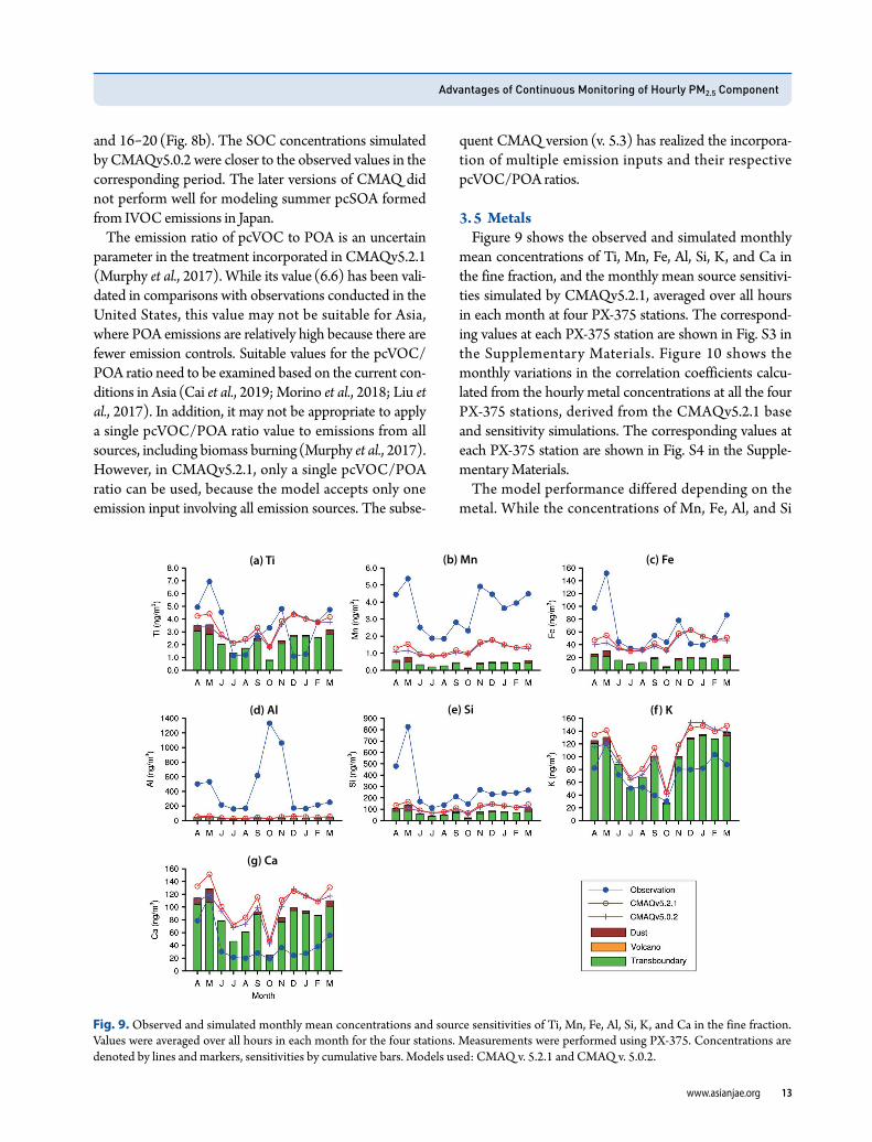
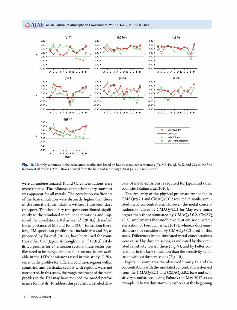
Figure 9 shows the observed and simulated monthly mean concentrations of Ti, Mn, Fe, Al, Si, K, and Ca in the fine fraction, and the monthly mean source sensitivi­ties simulated by CMAQv5.2.1, averaged over all hours in each month at four PX­375 stations. The correspond­ing values at each PX­375 station are shown in Fig. S3 in the Supplementary Materials. Figure 10 shows the monthly variations in the correlation coefficients calcu­lated from the hourly metal concentrations at all the four PX­375 stations, derived from the CMAQv5.2.1 base and sensitivity simulations. The corresponding values at each PX­375 station are shown in Fig. S4 in the Supple­mentary Materials.

The model performance differed depending on the metal. While the concentrations of Mn, Fe, Al, and Si

(a) Ti

(d) Al

(g) Ca

(b) Mn

(e) Si

(c) Fe

(f) K

Fig. 9. Observed and simulated monthly mean concentrations and source sensitivities of Ti, Mn, Fe, Al, Si, K, and Ca in the fine fraction. Values were averaged over all hours in each month for the four stations. Measurements were performed using PX­375. Concentrations are denoted by lines and markers, sensitivities by cumulative bars. Models used: CMAQ v. 5.2.1 and CMAQ v. 5.0.2.

Asian Journal of Atmospheric Environment, Vol. 15, No. 2, 2021008, 2021

14 www.asianjae.org

were all underestimated, K and Ca concentrations were overestimated. The influence of transboundary transport was apparent for all metals. The correlation coefficients of the base simulation were distinctly higher than those of the sensitivity simulation without transboundary transport. Transboundary transport contributed signifi­cantly to the simulated metal concentrations and imp­roved the correlations. Itahashi et al. (2018a) described the importance of Mn and Fe in SO4

2- formation; there­fore, PM speciation profiles that include Mn and Fe, as proposed by Fu et al. (2013), have been used for coun­tries other than Japan. Although Fu et al. (2013) estab­lished profiles for 24 emission sectors, these sector pro­files need to be merged into the four sectors that are avail ­ able in the HTAP emissions used in this study. Differ ­ en ces in the profiles for different countries, regions within countries, and particular sectors with regions, were not con sidered. In this study, the rough treatment of the metal profiles in the PM may have reduced the model per for ­ mance for metals. To address this problem, a detailed data ­

base of metal emissions is required for Japan and other countries (Kajino et al., 2020).

The similarity of the physical processes embedded in CMAQv5.2.1 and CMAQv5.0.2 resulted in similar simu­lated metal concentrations. However, the metal concen­trations simulated by CMAQv5.2.1 for May were much higher than those simulated by CMAQv5.0.2. CMAQ v5.2.1 implements the windblown dust emission param­eterization of Foroutan et al. (2017), whereas dust emis­sions are not considered by CMAQv5.0.2 used in this study. Differences in the simulated metal concentrations were caused by dust emissions, as indicated by the simu­lated sensitivity toward them (Fig. 9), and by better cor­relations in the base simulation than the sensitivity simu­lation without dust emissions (Fig. 10).

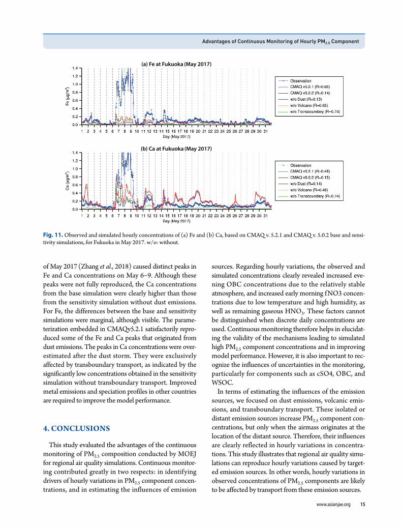
Figure 11 compares the observed hourly Fe and Ca con centrations with the simulated concentrations derived from the CMAQv5.2.1 and CMAQv5.0.2 base and sen­sitivity simulations, using Fukuoka in May 2017 as an exam ple. A heavy dust storm in east Asia at the beginning

Fig. 10. Monthly variations in the correlation coefficients based on hourly metal concentrations (Ti, Mn, Fe, Al, Si, K, and Ca) in the fine fraction at all four PX­375 stations derived from the base and sensitivity CMAQ v. 5.2.1 simulations.

(a) Ti

(d) Al

(g) Ca

(b) Mn

(e) Si

(c) Fe

(f) K

Advantages of Continuous Monitoring of Hourly PM2.5 Component

www.asianjae.org 15

of May 2017 (Zhang et al., 2018) caused distinct peaks in Fe and Ca concentrations on May 6­9. Although these peaks were not fully reproduced, the Ca concentrations from the base simulation were clearly higher than those from the sensitivity simulation without dust emissions. For Fe, the differences between the base and sensitivity simulations were marginal, although visible. The parame­terization embedded in CMAQv5.2.1 satisfactorily repro­duced some of the Fe and Ca peaks that originated from dust emissions. The peaks in Ca concentrations were over­ estimated after the dust storm. They were exclusively affected by transboundary transport, as indicated by the significantly low concentrations obtained in the sensitivity simulation without transboundary transport. Improved metal emissions and speciation profiles in other countries are required to improve the model performance.

4. CONCLUSIONS

This study evaluated the advantages of the continuous monitoring of PM2.5 composition conducted by MOEJ for regional air quality simulations. Continuous monitor­ing contributed greatly in two respects: in identifying drivers of hourly variations in PM2.5 component concen­trations, and in estimating the influences of emission

sources. Regarding hourly variations, the observed and simulated concentrations clearly revealed increased eve­ning OBC concentrations due to the relatively stable atmosphere, and increased early morning fNO3 concen­trations due to low temperature and high humidity, as well as remaining gaseous HNO3. These factors cannot be distinguished when discrete daily concentrations are used. Continuous monitoring therefore helps in elucidat­ing the validity of the mechanisms leading to simulated high PM2.5 component concentrations and in improving model performance. However, it is also important to rec­ognize the influences of uncertainties in the monitoring, particularly for components such as cSO4, OBC, and WSOC.

In terms of estimating the influences of the emission sources, we focused on dust emissions, volcanic emis­sions, and transboundary transport. These isolated or distant emission sources increase PM2.5 component con­centrations, but only when the airmass originates at the location of the distant source. Therefore, their influences are clearly reflected in hourly variations in concentra­tions. This study illustrates that regional air quality simu­lations can reproduce hourly variations caused by target­ed emission sources. In other words, hourly variations in observed concentrations of PM2.5 components are likely to be affected by transport from these emission sources.

Fig. 11. Observed and simulated hourly concentrations of (a) Fe and (b) Ca, based on CMAQ v. 5.2.1 and CMAQ v. 5.0.2 base and sensi­tivity simulations, for Fukuoka in May 2017. w/o: without.

(a) Fe at Fukuoka (May 2017)

(b) Ca at Fukuoka (May 2017)

Asian Journal of Atmospheric Environment, Vol. 15, No. 2, 2021008, 2021

16 www.asianjae.org

Using regional air quality simulations, this study rev­eals that continuous monitoring data is useful for identi­fying key processes and emission sources that increase PM2.5 component concentrations. Such data is likely to have various other purposes, including receptor model­ing. Continuous monitoring can contribute to the devel­opment of effective strategies for suppressing ambient PM2.5. It is therefore valuable to maintain and expand the continuous monitoring of PM2.5 compositions.

ACKNOWLEDGEMENT

This research was performed by the Environment Res­earch and Technology Development Fund ( JPMEERF 20165001 and JPMEERF20195003) of the Environmen ­ tal Restoration and Conservation Agency of Japan. The continuous monitoring data were obtained from the Mini ­ stry of the Environment of Japan (http://www.env.go.jp/air/%20osen/pm_resultmonitoring/post_25.html).

REFERENCES

Asano, H., Aoyama, T., Mizuno, Y., Shiraishi, Y. (2017) Highly Time­Resolved Atmospheric Observations Using a Continu­ous Fine Particulate Matter and Element Monitor. ACS Earth and Space Chemistry, 1(9), 580­590. https://doi.org/ 10.1021/acsearthspacechem.7b00090

Binkowski, F.S., Roselle, S.J. (2003) Models­3 Community Mul­tiscale Air Quality (CMAQ) Model Aerosol Component ­ 1. Model Description. Journal of Geophysical Research­Atmo­spheres, 108(D6), 4183. https://doi.org/10.1029/2001jd 001409

Byun, D., Schere, K.L. (2006) Review of the Governing Equa­tions, Computational Algorithms, and Other Components of the Models­3 Community Multiscale Air Quality (CMAQ) Modeling System. Applied Mechanics Reviews, 59(2), 51­ 77. https://doi.org/10.1115/1.2128636

Cai, S.Y., Zhu, L., Wang, S.X., Wisthaler, A., Li, Q., Jiang, J.K., Hao, J.M. (2019) Time­Resolved Intermediate­Volatility and Semivolatile Organic Compound Emissions from Household Coal Combustion in Northern China. Environmental Sci­ence & Technology, 53(15), 9269­9278. https://doi.org/ 10.1021/acs.est.9b00734

Carter, W.P.L. (2010) Development of the SAPRC­07 Chemi­cal Mechanism. Atmospheric Environment, 44(40), 5324­5335. https://doi.org/10.1016/j.atmosenv.2010.01.026

Chatani, S., Morino, Y., Shimadera, H., Hayami, H., Mori, Y., Sasaki, K., Kajino, M., Yokoi, T., Morikawa, T., Ohara, T. (2014) Multi­Model Analyses of Dominant Factors Influ­encing Elemental Carbon in Tokyo Metropolitan Area of Japan. Aerosol and Air Quality Research, 14(1), 396­405.

https://doi.org/10.4209/aaqr.2013.02.0035Chatani, S., Yamaji, K., Sakurai, T., Itahashi, S., Shimadera, H.,

Kitayama, K., Hayami, H. (2018) Overview of Model Inter­Comparison in Japan’s Study for Reference Air Quality Modeling ( J­STREAM). Atmosphere, 9(1), 19. https://doi.org/10.3390/atmos9010019

Chatani, S., Shimadera, H., Itahashi, S., Yamaji, K. (2020a) Com­prehensive Analyses of Source Sensitivities and Apportion­ments of PM2.5 and Ozone over Japan Via Multiple Numeri­cal Techniques. Atmospheric Chemistry and Physics, 20(17), 10311­10329. https://doi.org/10.5194/acp­20­10311­2020

Chatani, S., Yamaji, K., Itahashi, S., Saito, M., Takigawa, M., Mori­kawa, T., Kanda, I., Miya, Y., Komatsu, H., Sakurai, T., Morino, Y., Nagashima, T., Kitayama, K., Shimadera, H., Uranishi, K., Fujiwara, Y., Shintani, S., Hayami, H. (2020b) Identi fying Key Factors Influencing Model Performance on Ground­Level Ozone over Urban Areas in Japan through Model Inter­Com­parisons. Atmospheric Environment, 223, 117255. https://doi.org/10.1016/j.atmosenv.2019.117255

Choi, Y., Kanaya, Y., Park, S.M., Matsuki, A., Sadanaga, Y., Kim, S.W., Uno, I., Pan, X., Lee, M., Kim, H., Jung, D.H. (2020) Regional Variability in Black Carbon and Carbon Monoxide Ratio from Long­Term Observations over East Asia: Assess­ment of Representativeness for Black Carbon (BC) and Car­bon Monoxide (CO) Emission Inventories. Atmospheric Che mistry and Physics, 20(1), 83­98. https://doi.org/10. 5194/acp­20­83­2020

Clappier, A., Belis, C.A., Pernigotti, D., Thunis, P. (2017) Source Apportionment and Sensitivity Analysis: Two Method ­ ologies with Two Different Purposes. Geoscientific Model Development, 10(11), 4245­4256. https://doi.org/10. 5194/gmd­10­4245­2017

Dasgupta, P.K., Campbell, S.W., Al­Horr, R.S., Ullah, S.M.R., Li, J.Z., Amalfitano, C., Poor, N.D. (2007) Conversion of Sea Salt Aerosol to NaNO3 and the Production of HCl: Analysis of Temporal Behavior of Aerosol Chloride/Nitrate and Gas­eous HCl/HNO3 Concentrations with AIM. Atmospheric Environment, 41(20), 4242­4257. https://doi.org/10. 1016/j.atmosenv.2006.09.054

Donahue, N.M., Robinson, A.L., Stanier, C.O., Pandis, S.N. (2006) Coupled Partitioning, Dilution, and Chemical Aging of Semivolatile Organics. Environmental Science & Tech­nology, 40(8), 2635­2643. https://doi.org/10.1021/es052 297c

Emery, C., Liu, Z., Russell, A.G., Odman, M.T., Yarwood, G., Kumar, N. (2017) Recommendations on Statistics and Benchmarks to Assess Photochemical Model Performance. Journal of the Air & Waste Management Association, 67(5), 582­598. https://doi.org/10.1080/10962247.2016.1265027

Foroutan, H., Young, J., Napelenok, S., Ran, L., Appel, K.W., Gilliam, R.C., Pleim, J.E. (2017) Development and Evalua­tion of a Physics­Based Windblown Dust Emission Scheme Implemented in the CMAQ Modeling System. Journal of Advances in Modeling Earth Systems, 9(1), 585­608. https://doi.org/10.1002/2016ms000823

Fountoukis, C., Nenes, A. (2007) Isorropia Ii: A Computation­

Advantages of Continuous Monitoring of Hourly PM2.5 Component

www.asianjae.org 17

ally Efficient Thermodynamic Equilibrium Model for K+ ­ Ca2+ ­ Mg2+ ­ NH4

+ ­ Na+ ­ SO42- ­ NO3

- ­ Cl- ­ H2O Aero­sols. Atmospheric Chemistry and Physics, 7(17), 4639­4659. https://doi.org/10.5194/acp­7­4639­2007

Fu, X., Wang, S.X., Zhao, B., Xing, J., Cheng, Z., Liu, H., Hao, J.M. (2013) Emission Inventory of Primary Pollutants and Chemical Speciation in 2010 for the Yangtze River Delta Region, China. Atmospheric Environment, 70, 39­50. https://doi.org/10.1016/j.atmosenv.2012.12.034

Ikemori, F., Uranishi, K., Sato, T., Fujihara, M., Hasegawa, H., Sugata, S. (2021) Time­Resolved Characterization of Organic Compounds in PM2.5 Collected at Oki Island, Japan, Affected by Transboundary Pollution of Biomass and Non­Biomass Burning from Northeast China. Science of the Total Envi­ronment, 750, 142183. https://doi.org/10.1016/j.scitotenv. 2020.142183

Itahashi, S., Uno, I., Osada, K., Kamiguchi, Y., Yamamoto, S., Tamura, K., Wang, Z., Kurosaki, Y., Kanaya, Y. (2017) Nitrate Transboundary Heavy Pollution over East Asia in Winter. Atmospheric Chemistry and Physics, 17(6), 3823­3843. https://doi.org/10.5194/acp­17­3823­2017

Itahashi, S., Yamaji, K., Chatani, S., Hayami, H. (2018a) Refine­ment of Modeled Aqueous­Phase Sulfate Production Via the Fe­ and Mn­Catalyzed Oxidation Pathway. Atmosphere, 9(4), 132. https://doi.org/10.3390/atmos9040132

Itahashi, S., Yamaji, K., Chatani, S., Hisatsune, K., Saito, S., Hay­ami, H. (2018b) Model Performance Differences in Sulfate Aerosol in Winter over Japan Based on Regional Chemical Transport Models of CMAQ and CAMx. Atmosphere, 9(12), 488. https://doi.org/10.3390/atmos9120488

Itahashi, S., Yamaji, K., Chatani, S., Hayami, H. (2019) Differ­ences in Model Performance and Source Sensitivities for Sulfate Aerosol Resulting from Updates of the Aqueous­ and Gas­Phase Oxidation Pathways for a Winter Pollution Epi­sode in Tokyo, Japan. Atmosphere, 10(9), 544. https://doi.org/10.3390/atmos10090544

Itahashi, S., Wang, Z., Yumimoto, K., Uno, I. (2020a) Drastic Changes of PM2.5 Trans­Boundary Pollution over Japan Due to COVID­19 Lockdown in China. Journal of Japan Society for Atmospheric Environment/Taiki Kankyo Gakkaishi, 55(6), 239­247. https://doi.org/10.11298/taiki.55.239

Itahashi, S., Yamaji, K., Chatani, S., Kitayama, K., Morino, Y., Nagashima, T., Saito, M., Takigawa, M., Morikawa, T., Kanda, I., Miya, Y., Komatsu, H., Sakurai, T., Shimadera, H., Uranishi, K., Fujiwara, Y., Hashimoto, T., Hayami, H. (2020b) Model Performance Differences in Fine­Mode Nitrate Aerosol Dur­ing Wintertime over Japan in the J­STREAM Model Inter­Comparison Study. Atmosphere, 11(5), 511. https://doi.org/10.3390/atmos11050511

Janssens­Maenhout, G., Crippa, M., Guizzardi, D., Dentener, F., Muntean, M., Pouliot, G., Keating, T., Zhang, Q., Kurokawa, J., Wankmuller, R., van der Gon, H.D., Kuenen, J.J.P., Kli­mont, Z., Frost, G., Darras, S., Koffi, B., Li, M. (2015) HTAP_V2.2: A Mosaic of Regional and Global Emission Grid Maps for 2008 and 2010 to Study Hemispheric Trans­port of Air Pollution. Atmospheric Chemistry and Physics, 15(19), 11411­11432. https://doi.org/10.5194/acp­15­11411­2015

Kajino, M., Sato, K., Inomata, Y., Ueda, H. (2013) Source­Recep­tor Relationships of Nitrate in Northeast Asia and Influence of Sea Salt on the Long­Range Transport of Nitrate. Atmo­spheric Environment, 79, 67­78. https://doi.org/10.1016/j.atmosenv.2013.06.024

Kajino, M., Hagino, H., Fujitani, Y., Morikawa, T., Fukui, T., Onishi, K., Okuda, T., Kajikawa, T., Igarashi, Y. (2020) Mod­eling Transition Metals in East Asia and Japan and Its Emis­sion Sources. Geohealth, 4(9), e2020GH000259. https://doi.org/10.1029/2020gh000259

Kanaya, Y., Yamaji, K., Miyakawa, T., Taketani, F., Zhu, C., Choi, Y., Komazaki, Y., Ikeda, K., Kondo, Y., Klimont, Z. (2020) Rapid Reduction in Black Carbon Emissions from China: Evidence from 2009­2019 Observations on Fukue Island, Japan. Atmospheric Chemistry and Physics, 20(11), 6339­6356. https://doi.org/10.5194/acp­20­6339­2020

Kelly, J.T., Bhave, P.V., Nolte, C.G., Shankar, U., Foley, K.M. (2010) Simulating Emission and Chemical Evolution of Coarse Sea­Salt Particles in the Community Multiscale Air Quality (CMAQ) Model. Geoscientific Model Development, 3(1), 257­273. https://doi.org/10.5194/gmd­3­257­2010

Kojima, S., Michikawa, T., Matsui, K., Ogawa, H., Yamazaki, S., Nitta, H., Takami, A., Ueda, K., Tahara, Y., Yonemoto, N., Nonogi, H., Nagao, K., Ikeda, T., Sato, N., Tsutsui, H. (2020) Association of Fine Particulate Matter Exposure with Bystan ­ der­Witnessed out­of­Hospital Cardiac Arrest of Cardiac Ori­gin in Japan. JAMA Network Open, 3(4), e203043. https://doi.org/10.1001/jamanetworkopen.2020.3043

Kondo, Y., Miyazaki, Y., Takegawa, N., Miyakawa, T., Weber, R.J., Jimenez, J.L., Zhang, Q., Worsnop, D.R. (2007) Oxygenated and Water­Soluble Organic Aerosols in Tokyo. Journal of Geophysical Research­Atmospheres, 112(D1), D01203. https://doi.org/10.1029/2006jd007056

Li, Y.Y., Chang, M.A., Ding, S.S., Wang, S.W., Ni, D., Hu, H.T. (2017) Monitoring and Source Apportionment of Trace Ele­ments in PM2.5: Implications for Local Air Quality Manage­ment. Journal of Environmental Management, 196, 16­25. https://doi.org/10.1016/j.jenvman.2017.02.059

Liu, H., Man, H.Y., Cui, H.Y., Wang, Y.J., Deng, F.Y., Wang, Y., Yang, X.F., Xiao, Q., Zhang, Q., Ding, Y., He, K.B. (2017) An Updated Emission Inventory of Vehicular Vocs and Ivocs in China. Atmospheric Chemistry and Physics, 17(20), 12709­ 12724. https://doi.org/10.5194/acp­17­12709­2017

Ministry of the Environment (2020) https://www.env.go.jp/air/osen/index.html (Last access: December 3rd, 2020).

Miyazaki, Y., Kondo, Y., Takegawa, N., Komazaki, Y., Fukuda, M., Kawamura, K., Mochida, M., Okuzawa, K., Weber, R.J. (2006) Time­Resolved Measurements of Water­Soluble Org ­ anic Carbon in Tokyo. Journal of Geophysical Research­Atmo ­ s pheres, 111(D23), D23206. https://doi.org/10.1029/2006 jd007125

Morino, Y., Nagashima, T., Sugata, S., Sato, K., Tanabe, K., Nogu­chi, T., Takami, A., Tanimoto, H., Ohara, T. (2015) Verifica­tion of Chemical Transport Models for PM2.5 Chemi ­ cal Composition Using Simultaneous Measurement Data over Japan. Aerosol and Air Quality Research, 15(5), 2009­2023. https://doi.org/10.4209/aaqr.2015.02.0120

Morino, Y., Chatani, S., Tanabe, K., Fujitani, Y., Morikawa, T.,

Asian Journal of Atmospheric Environment, Vol. 15, No. 2, 2021008, 2021

18 www.asianjae.org

Takahashi, K., Sato, K., Sugata, S. (2018) Contributions of Condensable Particulate Matter to Atmospheric Organic Aero­sol over Japan. Environmental Science & Technology, 52(15), 8456­8466. https://doi.org/10.1021/acs.est.8b01285

Murphy, B.N., Woody, M.C., Jimenez, J.L., Carlton, A.M.G., Hayes, P.L., Liu, S., Ng, N.L., Russell, L.M., Setyan, A., Xu, L., Young, J., Zaveri, R.A., Zhang, Q., Pye, H.O.T. (2017) Semi­volatile POA and Parameterized Total Combustion SOA in Cmaqv5.2: Impacts on Source Strength and Partitioning. Atmospheric Chemistry and Physics, 17(18), 11107­ 11133. https://doi.org/10.5194/acp­17­11107­2017

Nakatsubo, R., Horie, Y., Takimoto, M., Matsumura, C., Hiraki, T. (2018) Analysis of Hourly Observation Data of PM2.5 Che ­ mical Components at a Coastal Area in Seto Inland Sea. Earo­zoru Kenkyu, 33(3), 175­182. https://doi.org/10.11203/jar.33.175

Nenes, A., Pandis, S.N., Weber, R.J., Russell, A. (2020) Aerosol Ph and Liquid Water Content Determine When Particulate Matter Is Sensitive to Ammonia and Nitrate Availability. Atmospheric Chemistry and Physics, 20(5), 3249­3258. https://doi.org/10.5194/acp­20­3249­2020

Osada, K., Kamiguchi, Y., Yamamoto, S., Kuwahara, S., Pan, X., Hara, Y., Uno, I. (2016) Comparison of Ionic Concentrations on Size­Segregated Atmospheric Aerosol Particles Based on a Denuder­Filter Method and a Continuous Dichotomous Aerosol Chemical Speciation Analyzer (ACSA­12). Earozoru Kenkyu, 31(3), 203­209. https://doi.org/10.11203/jar.31. 203

Otte, T.L., Pleim, J.E. (2010) The Meteorology­Chemistry Inter­face Processor (MCIP) for the CMAQ Modeling System: Updates through Mcipv3.4.1. Geoscientific Model Develop­ment, 3(1), 243­256. https://doi.org/10.5194/gmd­3­243­2010

Pan, X.L., Ge, B.Z., Wang, Z., Tian, Y., Liu, H., Wei, L.F., Yue, S.Y., Uno, I., Kobayashi, H., Nishizawa, T., Shimizu, A., Fu, P.Q., Wang, Z.F. (2019) Synergistic Effect of Water­Soluble Species and Relative Humidity on Morphological Changes in Aerosol Particles in the Beijing Megacity During Severe Pollution Episodes. Atmospheric Chemistry and Physics, 19(1), 219­232. https://doi.org/10.5194/acp­19­219­2019

Pleim, J.E. (2007) A Combined Local and Nonlocal Closure Model for the Atmospheric Boundary Layer. Part I: Model Des cription and Testing. Journal of Applied Meteorology and Climatology, 46(9), 1383­1395. https://doi.org/10.1175/jam2539.1

Ramboll Environ (2016) CAMx User’s Guide Version 6.40. http://www.camx.com/files/camxusersguide_v6­40.pdf

Robinson, A.L., Donahue, N.M., Shrivastava, M.K., Weitkamp, E.A., Sage, A.M., Grieshop, A.P., Lane, T.E., Pierce, J.R., Pan­dis, S.N. (2007) Rethinking Organic Aerosols: Semivolatile Emissions and Photochemical Aging. Science, 315(5816), 1259. https://doi.org/10.1126/science.1133061

Saito, S., Hoshi, J., Ikemori, F., Osada, K. (2020) Comparison of Water­Soluble Organic Carbon in PM2.5 Obtained by Filter Analysis and Continuous Dichotomous Aerosol Chemical Speciation Analyzer. Journal of Japan Society for Atmospheric Environment/Taiki Kankyo Gakkaishi, 55(3), 150­158. https://doi.org/10.11298/taiki.55.150

Shimadera, H., Hayami, H., Chatani, S., Morino, Y., Mori, Y., Morikawa, T., Yamaji, K., Ohara, T. (2014) Sensitivity Analy­ses of Factors Influencing CMAQ Performance for Fine Par­ticulate Nitrate. Journal of the Air & Waste Management Association, 64(4), 374­387. https://doi.org/10.1080/10962247.2013.778919

Sudo, K., Takahashi, M., Kurokawa, J., Akimoto, H. (2002) CHASER: A Global Chemical Model of the Troposphere ­ 1. Model Description. Journal of Geophysical Research­Atmo­spheres, 107(D17), 4339. https://doi.org/10.1029/2001jd 001113

Uno, I., Osada, K., Yumimoto, K., Wang, Z., Itahashi, S., Pan, X.L., Hara, Y., Kanaya, Y., Yamamoto, S., Fairlie, T.D. (2017a) Seasonal Variation of Fine­ and Coarse­Mode Nitrates and Related Aerosols over East Asia: Synergetic Observations and Chemical Transport Model Analysis. Atmospheric Chemis­try and Physics, 17(23), 14181­14197. https://doi.org/10. 5194/acp­17­14181­2017

Uno, I., Osada, K., Yumimoto, K., Wang, Z., Itahashi, S., Pan, X.L., Hara, Y., Yamamoto, S., Nishizawa, T. (2017b) Impor­tance of Long­Range Nitrate Transport Based on Long­Term Observation and Modeling of Dust and Pollutants over East Asia. Aerosol and Air Quality Research, 17(12), 3052­3064. https://doi.org/10.4209/aaqr.2016.11.0494

Uno, I., Wang, Z., Itahashi, S., Yumimoto, K., Yamamura, Y., Yoshino, A., Takami, A., Hayasaki, M., Kim, B.­G. (2020) Paradigm Shift in Aerosol Chemical Composition over Reg­ions Downwind of China. Scientific Reports, 10(1), 6450. https://doi.org/10.1038/s41598­020­63592­6

Uranishi, K., Ikemori, F., Nakatsubo, R., Shimadera, H., Kondo, A., Kikutani, Y., Asano, K., Sugata, S. (2017) Identification of Biased Sectors in Emission Data Using a Combination of Chemical Transport Model and Receptor Model. Atmosphe­ric Environment, 166, 166­181. https://doi.org/10.1016/j.atmosenv.2017.06.039

Yamaji, K., Chatani, S., Itahashi, S., Saito, M., Takigawa, M., Mor­ikawa, T., Kanda, I., Miya, Y., Komatsu, H., Sakurai, T., Mori­no, Y., Kitayama, K., Nagashima, T., Shimadera, H., Uranishi, K., Fujiwara, Y., Hashimoto, T., Sudo, K., Misaki, T., Hayami, H. (2020) Model Inter­Comparison for PM2.5 Components over Urban Areas in Japan in the J­STREAM Framework. Atmosphere, 11(3), 222. https://doi.org/10.3390/atmos11 030222

Yan, C.Q., Zheng, M., Sullivan, A.P., Bosch, C., Desyaterik, Y., Andersson, A., Li, X.Y., Guo, X.S., Zhou, T., Gustafsson, O., Collett, J.L. (2015) Chemical Characteristics and Light­Absorbing Property of Water­Soluble Organic Carbon in Bei­jing: Biomass Burning Contributions. Atmospheric Environ­ment, 121, 4­12. https://doi.org/10.1016/j.atmosenv.2015. 05.005

Ye, S.Q., Ma, T., Duan, F.K., Li, H., He, K.B., Xia, J., Yang, S., Zhu, L.D., Ma, Y.L., Huang, T., Kimoto, T. (2019) Characteristics and Formation Mechanisms of Winter Haze in Changzhou, a Highly Polluted Industrial City in the Yangtze River Delta, China. Environmental Pollution, 253, 377­383. https://doi.org/10.1016/j.envpol.2019.07.011

Zhang, L., Brook, J.R., Vet, R. (2003) A Revised Parameteriza­tion for Gaseous Dry Deposition in Air­Quality Models.

Advantages of Continuous Monitoring of Hourly PM2.5 Component

www.asianjae.org 19

Atmospheric Chemistry and Physics, 3(6), 2067­2082. https://doi.org/10.5194/acp­3­2067­2003

Zhang, X.X., Sharratt, B., Liu, L.Y., Wang, Z.F., Pan, X.L., Lei, J.Q., Wu, S.X., Huang, S.Y., Guo, Y.H., Li, J., Tang, X., Yang, T., Tian, Y., Chen, X.S., Hao, J.Q., Zheng, H.T., Yang, Y.Y., Lyu,

Y.L. (2018) East Asian Dust Storm in May 2017: Observa­tions, Modelling, and Its Influence on the Asia­Pacific Reg ion. Atmospheric Chemistry and Physics, 18(11), 8353­8371. https://doi.org/10.5194/acp­18­8353­2018

Asian Journal of Atmospheric Environment, Vol. 15, No. 2, 2021008, 2021

20 www.asianjae.org

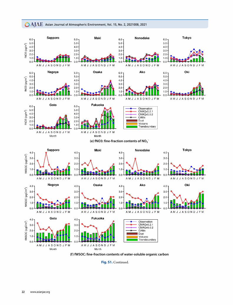
Fig. S1. Air quality parameters at the ten ACSA­14 stations, giving the observed and simulated monthly mean concentrations and source sensitivities. The values were averaged over all hours in each month. Concentrations are denoted by lines and markers; sensitivities by cumulative bars. Models used: CMAQ v. 5.2.1 and 5.0.2, and CAMx.

(a) PM2.5: ambient fine particulate matter<2.5 μm

(b) PMc: coarse-fraction PM

SUPPLEMENTARY MATERIALS

Advantages of Continuous Monitoring of Hourly PM2.5 Component

www.asianjae.org 21

(c) OBC: fine-fraction contents of optically measured black carbon

(d) fSO4: fine-fraction contents of SO42-

Fig. S1. Continued.

Asian Journal of Atmospheric Environment, Vol. 15, No. 2, 2021008, 2021

22 www.asianjae.org

(e) fNO3: fine-fraction contents of NO3-

(f) fWSOC: fine-fraction contents of water-soluble organic carbon

Fig. S1. Continued.

Advantages of Continuous Monitoring of Hourly PM2.5 Component

www.asianjae.org 23

(g) cSO4: coarse-fraction contents of SO42-

(h) cNO3: coarse-fraction contents of NO3-

Fig. S1. Continued.

Asian Journal of Atmospheric Environment, Vol. 15, No. 2, 2021008, 2021

24 www.asianjae.org

(a) PM2.5: ambient fine particulate matter<2.5 μm

(b) PMc: coarse-fraction PM

Fig. S2. Monthly variation in correlation coefficients of air quality parameters at the ten ACSA­14 stations, based on hourly concentrations of particulate matter (PM) and its components simulated using CMAQ v. 5.2.1 in the base and sensitivity simulations. w/o: without.

Advantages of Continuous Monitoring of Hourly PM2.5 Component

www.asianjae.org 25

(c) OBC: fine-fraction contents of optically measured black carbon

(d) fSO4: fine-fraction contents of SO42-

Fig. S2. Continued.

Asian Journal of Atmospheric Environment, Vol. 15, No. 2, 2021008, 2021

26 www.asianjae.org

(e) fNO3: fine-fraction contents of NO3-

(f) fWSOC: fine-fraction contents of water-soluble organic carbon

Fig. S2. Continued.

Advantages of Continuous Monitoring of Hourly PM2.5 Component

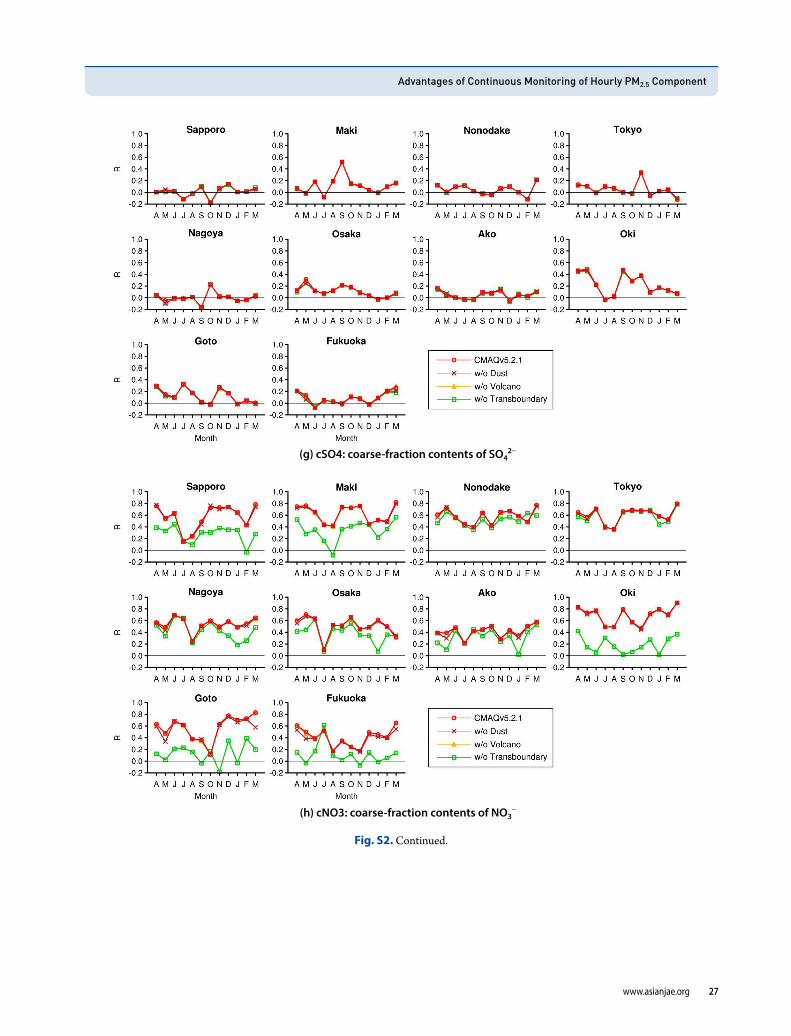
www.asianjae.org 27

(g) cSO4: coarse-fraction contents of SO42-

(h) cNO3: coarse-fraction contents of NO3-

Fig. S2. Continued.

Asian Journal of Atmospheric Environment, Vol. 15, No. 2, 2021008, 2021

28 www.asianjae.org

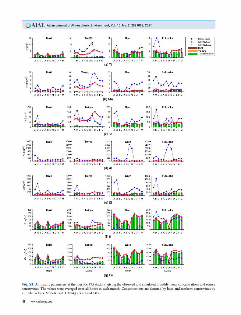
Fig. S3. Air quality parameters at the four PX­375 stations, giving the observed and simulated monthly mean concentrations and source sensitivities. The values were averaged over all hours in each month. Concentrations are denoted by lines and markers; sensitivities by cumulative bars. Models used: CMAQ v. 5.2.1 and 5.0.2.

(b) Mn

(c) Fe

(d) Al

(e) Si

(f) K

(a) Ti

(g) Ca

Advantages of Continuous Monitoring of Hourly PM2.5 Component

www.asianjae.org 29

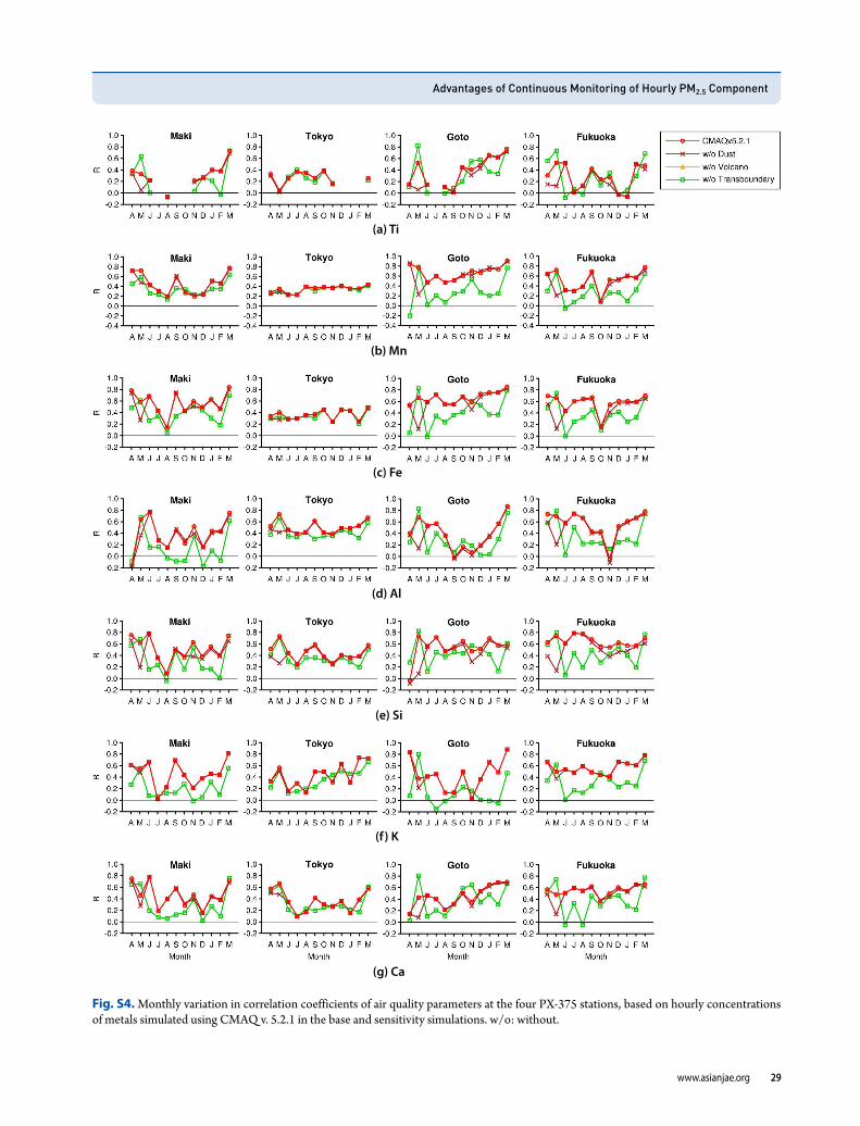
(a) Ti

(b) Mn

(c) Fe

(d) Al

(e) Si

(f) K

Fig. S4. Monthly variation in correlation coefficients of air quality parameters at the four PX­375 stations, based on hourly concentrations of metals simulated using CMAQ v. 5.2.1 in the base and sensitivity simulations. w/o: without.

(g) Ca