Advances of Soft Computing Methods in Edge Detection

Int. J. Advance. Soft Comput. Appl., Vol. 1, No. 2, November 2009 ISSN 2074-8523; Copyright © ICSRS Publication, 2009 www.i-csrs.org

Advances of Soft Computing Methods in Edge Detection

Amir Atapour Abarghouei, Afshin Ghanizadeh, and Siti Mariyam Shamsuddin

Soft Computing Research Group Universiti Teknologi Malaysia

Skudai, Johor Bahru e-mail: [email protected], [email protected],

[email protected]

Abstract

Artificial Intelligence (AI) techniques are now commonly used to solve complex and ill-defined problems. AI a broad field and will bring different meanings for different people. John McCarthy would probably use AI as “computational intelligence”, while Zadeh claimed that computational intelligence is actually Soft Computing (SC) techniques. Regardless of its definition, AI concerns with tasks that require human intelligence which require complex and advanced reasoning processes and knowledge. Due to its ability to learn, handle incomplete or incomprehensible data, deal with non-linear problems, and perform reasonable tasks very fast, AI has been used in diverse applications in control, robotics, pattern recognition, forecasting, medicine, power systems, manufacturing, optimization, signal processing, and social sciences. However, in this paper, we will focus on Soft Computing (SC), one of the AI influences that sprang from the concept of cybernetics. The main objective of this paper is to illustrate how some of these SC techniques generally work on detecting the edges. The paper also outlines practical differences among these techniques when they are applied to solving the problem of edge detection.

Keywords: Artificial Intelligence, Soft Computing, Ant Colony Optimization, Gravitational Search Algorithm, Edge Detection.

163 Advances of Soft Computing methods in Edge Detection

1 Introduction

The term Artificial Intelligence (AI) refers to the intelligence of machines. Conventional AI research focuses on an attempt to mimic human intelligent behavior by expressing it in language forms or symbolic rules. Conventional AI basically manipulates symbols on the assumption that such behavior can be stored in symbolically structured knowledge bases. Perhaps the most successful conventional AI product is the knowledge-based system or expert system (ES). Through many years of research, a large number of techniques have been developed in the field of AI to solve the most difficult problems in computer science. However, it should be noted that merely solving a problem does not indicate complete understanding of a situation. Understanding is one the main requirements for intelligence. Therefore an AI technique, by which even difficult problems are solved, still doesn’t provide actual intelligence. On the other hand, modern AI inevitably depends on personal judgment, and it is true that many books on modern AI describe neural networks and perhaps other soft computing components.

Soft Computing can be considered as a field dedicated to problem solving methods capable of simultaneously exploiting numerical data and human knowledge, using mathematical modeling and symbolic reasoning systems. It is tolerant of imprecision, uncertainty, and partial truth. The SOUL of SC is to make computers as SOFT as the human brain, and is capable of carrying out both quantitative information that takes the form of precise numerical and qualitative information that assumes qualitative statements of knowledge and experience represented by natural languages.

SC components consist of several major branches, and many of these techniques were inspired by the activities of the human brain, the behavior of animals, and laws of nature. In this paper, some of the most important SC techniques are given and these include Fuzzy Sets, Artificial Neural Networks (ANN), Genetic Algorithm (GA), Ant Colony Optimization (ACO) and Gravitational Search Algorithm (GSA). These techniques have been proven to be efficient in solving various complex problems. In depth discussion on each of these techniques is given in the next section. The rest of the paper is organized as follows: Section 2 provides discussions on Fuzzy Sets, ANN, GA, ACO, GSA, and their applications. Section 3 provides a comparison of these techniques on edge detection, and finally Section 4 concludes the paper and suggests some possible research work for the future.

Amir Atapour et al. 164

2 Soft Computing Methods

In this section, five major SC components are discussed. These include Fuzzy Sets, Artificial Neural Networks, Genetic Algorithm, Ant Colony Optimization, and Gravitational Search Algorithm.

2.1 Genetic Algorithm

Genetic Algorithm (GA) is a search method that is used to find the exact or, in most cases, the approximate solutions for optimization and search problems. Basically, GA is a heuristic optimization method, inspired from biological mechanisms of evolution and natural genetics. Unlike other search methods [2][3][4], Holland [1] proposed GA, an evolutionary algorithm that does not take the basic approach of heading downhill from an arbitrary starting point. For better understanding of GA concept, we need to understand the process of biological evolution, and this is discussed in the next sub-section.

2.1.1 Biological Evolution

In nature, competition among individuals for resources such as food and space leads to the domination of strong individuals over the weaker ones. Only the fittest individuals survive and reproduce. Hence, the genes of the fittest survive. The process of reproduction creates diversity in the gene pool. Evolution is the result of two individual chromosomes combining during reproduction. New combinations of genes are created from previous ones and a new gene pool is generated. When the genetic material is exchanged between the chromosomes of the two parents, a “crossover” has happened which might result in the creation of a fitter individual. Repeated selection (Survival of the fittest) and crossover cause the continuous evolution and therefore generation of individuals that survive better in a competitive environment or in a sense, are fitter. Mutation is another phenomenon in genetic, which causes sporadic and random alterations in genes and can help to regenerate lost genetic materials [5].

A Simple Genetic Algorithm (SGA) has been proposed by Holland [1]. This algorithm works with binary strings; the encoded versions of a solution to the optimization problem. The algorithm produces a secondary generation of strings using the genetic operators (crossover and mutation) and the cycle is repeated until a termination condition is reached. The population that undergoes the process of evolution in each cycle is chosen according to the fitness of chromosomes. The algorithm of SGA is given below.

Simple Genetic Algorithm: Simple Genetic Algorithm() { initial population; evaluate population;


WHILE termination conditions not met do select solutions for next population; perform crossover and mutation; evaluate population; END WHILE }

2.2 Advances in Genetic Algorithm

Genetic Algorithm works well for many practical problems. However, in complex design, simple GA may converge extremely slowly or it may fail, due to convergence to an unacceptable local optimum. Considerable research efforts have been made to improve GA. Some of these improvements are mentioned below.

2.2.1 Multi-Objective Genetic Algorithm

Common goal of problem solving in engineering is to obtain a good performance and low cost solution, and this constitute to two conflicting objectives. Therefore, the usage of multi objective optimization arises to solve multi solutions. Schaffer [14] improves the SGA with a selection mechanism that takes multiple objectives into consideration. Each generation includes a number of sub-populations that are selected based on one objective function. Subsequently, the sub-populations are mixed to obtain one population.

2.2.2 Parallel Genetic Algorithm

Parallel GAs is usually used when the evaluation of the fitness function is extremely time-consuming. Parallel GAs can be achieved using several different methods, and one of the most common approaches is to use a simple master-slave scheme. A simple master-slave uses one processor, which is called as the master. This master stores the population while the other processors (the slaves) evaluate the individuals and perform reproduction operators. Cantu-paz [15] provides a better comprehensive overview of parallel GAs.

2.2.3 Diversity Maintenance

It was mentioned previously that the mutation operator is applied in order to guarantee the diversity in GAs. However, even with proper use of mutation, in later generations, the population begins to converge, the individuals become similar and the population may converge to an unacceptable solution [16]. Having premature convergence leads to an unacceptable local optimum. Niching methods [16,17,18,19,20,21,22] maintain the diversity by keeping the population individuals away from each other (refer to [20] for detail discussion of Niching methods).


2.2.4 Applications of Genetic Algorithm

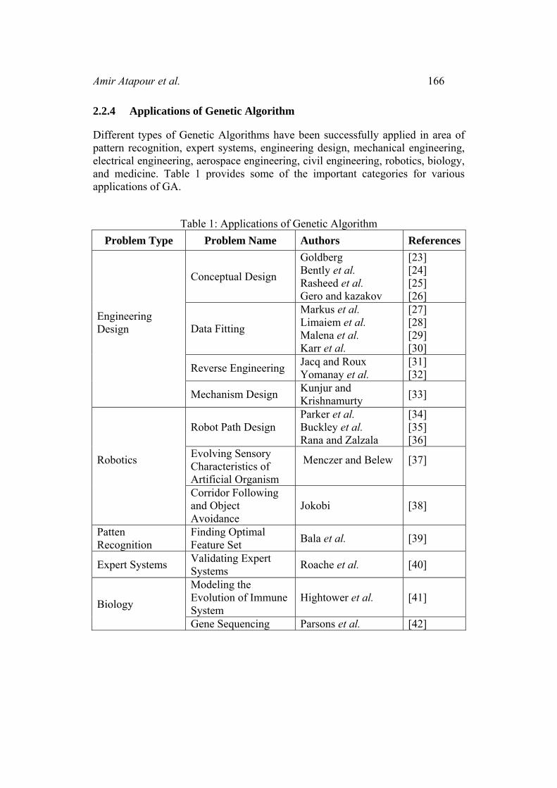
Different types of Genetic Algorithms have been successfully applied in area of pattern recognition, expert systems, engineering design, mechanical engineering, electrical engineering, aerospace engineering, civil engineering, robotics, biology, and medicine. Table 1 provides some of the important categories for various applications of GA.

Table 1: Applications of Genetic Algorithm Problem Type Problem Name Authors References

Engineering Design

Conceptual Design

Goldberg Bently et al. Rasheed et al. Gero and kazakov

[23] [24] [25] [26]

Data Fitting

Markus et al. Limaiem et al. Malena et al. Karr et al.

[27] [28] [29] [30]

Reverse Engineering Jacq and Roux Yomanay et al.

[31] [32]

Mechanism Design Kunjur and Krishnamurty [33]

Robotics

Robot Path Design Parker et al. Buckley et al. Rana and Zalzala

[34] [35] [36]

Evolving Sensory Characteristics of Artificial Organism

Menczer and Belew

[37]

Corridor Following and Object Avoidance

Jokobi [38]

Patten Recognition

Finding Optimal Feature Set Bala et al. [39]

Expert Systems Validating Expert Systems Roache et al. [40]

Biology

Modeling the Evolution of Immune System

Hightower et al. [41]

Gene Sequencing Parsons et al. [42]


2.3 Ant Colony Optimization

One of the new problem solving approaches that takes inspiration from the social behavior of insects and other animals is swarm intelligence. Particle Swarm Optimization (PSO) was first proposed by Kennedy and Eberhart [43] in 1995 and was taken from the social behavior of groups, where members behave based on both themselves and the group’s best interest. Ant Colony Optimization (ACO) is another swarm intelligence technique which was first introduce by Dorigo et al. [44,45,46]. ACO has attracted the attention of an increasing number of researchers and many successful applications are now available. The inspiration source of ACO is the foraging behavior of ants. In the next section, we discuss the basic concepts of ACO for a better understanding of ants’ behavior.

2.3.1 Biological Inspiration

In the 1940s, Pierre-Paul Grasse [47] first realized that species of termites react to what he called “Significant Stimuli”. These reactions take place both in the insects that produced them and for the other insects in the colony. The term “Stigmetry” [48] was introduce by Grass, describes an indirect communication amongst a self-organizing system like an insect colony via individuals modifying their local environment, which means it can only be accessed by the insect visiting the locus in which the modification happened. Stigmetry can be observed in colonies of ants. When ants are in search of a food resource, they leave a substance called pheromone behind as they move. Other ants perceive the presence of the already deposited pheromone and tend to follow the paths where pheromone concentration is higher. Deneuboury et al. [49] has investigated the process of pheromone laying and ant behavior thoroughly.

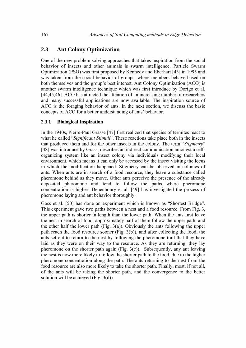
Goss et al. [50] has done an experiment which is known as “Shortest Bridge”. This experiment gave two paths between a nest and a food resource. From Fig. 3, the upper path is shorter in length than the lower path. When the ants first leave the nest in search of food, approximately half of them follow the upper path, and the other half the lower path (Fig. 3(a)). Obviously the ants following the upper path reach the food resource sooner (Fig. 3(b)), and after collecting the food, the ants set out to return to the nest by following the pheromone trail that they have laid as they were on their way to the resource. As they are returning, they lay pheromone on the shorter path again (Fig. 3(c)). Subsequently, any ant leaving the nest is now more likely to follow the shorter path to the food, due to the higher pheromone concentration along the path. The ants returning to the nest from the food resource are also more likely to take the shorter path. Finally, most, if not all, of the ants will be taking the shorter path, and the convergence to the better solution will be achieved (Fig. 3(d)).


Fig. 3. A schematic illustration of the ‘‘Shortest bridge” experiment.

By using simple computational Agents that work cooperatively, and communicate through artificial pheromone trails, just as the ants do in nature, we can simulate the ant colony behavior to solve optimization problems [51].

2.3.2 The Original Ant System

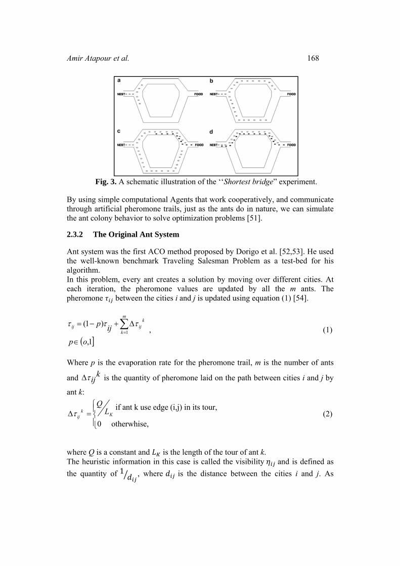
Ant system was the first ACO method proposed by Dorigo et al. [52,53]. He used the well-known benchmark Traveling Salesman Problem as a test-bed for his algorithm. In this problem, every ant creates a solution by moving over different cities. At each iteration, the pheromone values are updated by all the m ants. The pheromone between the cities i and j is updated using equation (1) [54].

( ]1,

)1(1

op

ijpm

k

kijij

∈

∆+−= ∑=

τττ , (1)

Where p is the evaporation rate for the pheromone trail, m is the number of ants

and kijτ∆ is the quantity of pheromone laid on the path between cities i and j by

ant k:

if ant k use edge (i,j) in its tour,

0 otherwhise,

kKij

QLτ

⎧⎪∆ = ⎨⎪⎩

(2)

where Q is a constant and is the length of the tour of ant k. The heuristic information in this case is called the visibility and is defined as the quantity of 1 , where is the distance between the cities i and j. As


opposed to the pheromone trail, this quantity is not modified during the algorithm when ant k is in city i and has constructed the partial solution S so fair.

2.3.3 Ant Algorithm as a Computational Optimization Technique

The ACO metaheuristic [55] was developed subsequent to the efficiency of Ant System in solving the Traveling Salesman Problem. ACO metaheuristic is used to solve the combinatorial problems based on the natural behavior of ants.

ACO algorithm consists of three mail function (Algorithm 2).

a. Autosolutionconstruct ( ) performs the process of constructing a solution as the following: Artificial ants move through adjacent states of a problem according to a transition rule, and create solutions iteratively.

b. PheromkoneUpdate ( ) updates the pheromone trails either after the complete solutions have been constructed or after each iteration, depending on the problem. In early stages of the algorithm run, ACO finds bad and unacceptable solutions as well as the good solution. In order to leave the bad solution behind, ACO includes pheromone trail evaporation. By reducing all the pheromone trails after the completion of each ant construction, the important feature can easily be implemented.

c. DeamonAction ( ) is an optional step in the algorithm which involves additional update parameters from a global perspective [51]. An example could be applying additional pheromone reinforcement to the best solution generated.

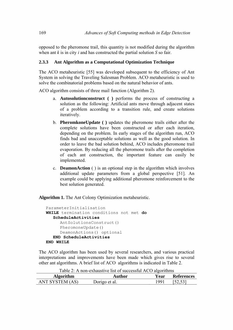
Algorithm 1. The Ant Colony Optimization metaheuristic.

ParameterInitialisation WHILE termination conditions not met do

ScheduleActivities AntSolutionsConstruct() PheromoneUpdate() DeamonActions() optional

END ScheduleActivities END WHILE

The ACO algorithm has been used by several researchers, and various practical interpretations and improvements have been made which gives rise to several other ant algorithms. A brief list of ACO algorithms is indicated in Table 2.

Table 2: A non-exhaustive list of successful ACO algorithms Algorithm Author Year References

ANT SYSTEM (AS) Dorigo et al. 1991 [52,53]


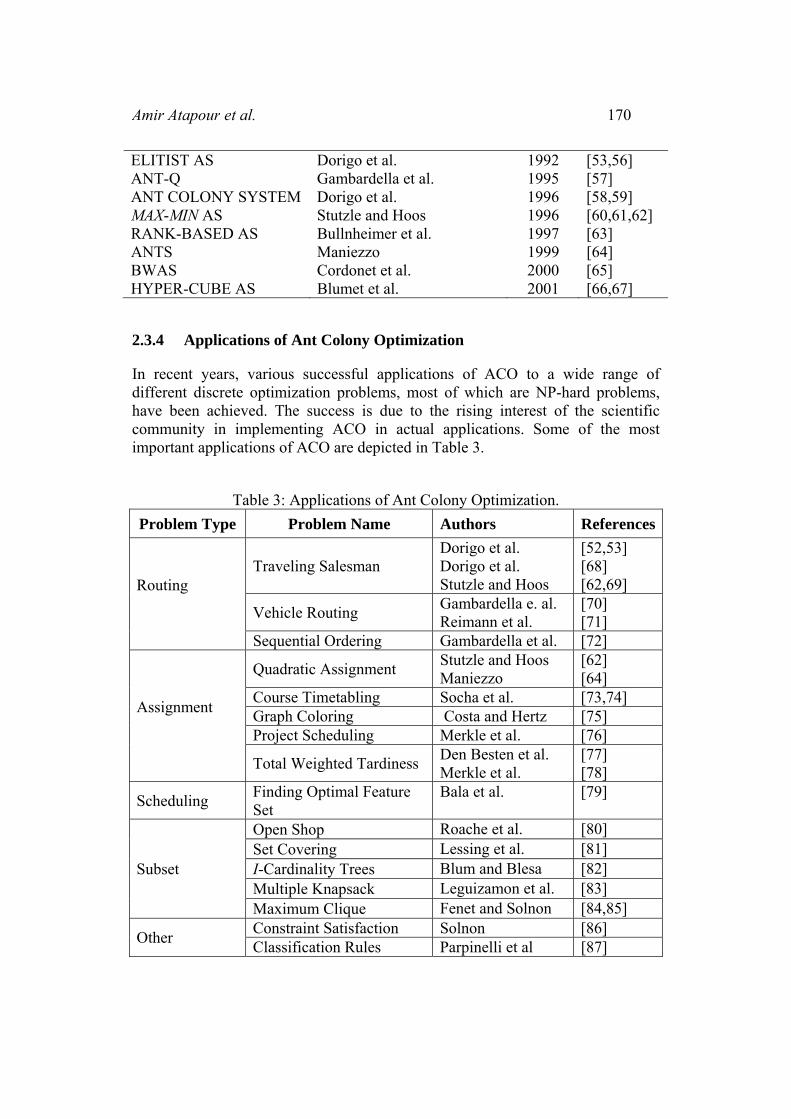
ELITIST AS Dorigo et al. 1992 [53,56] ANT-Q Gambardella et al. 1995 [57] ANT COLONY SYSTEM Dorigo et al. 1996 [58,59] MAX-MIN AS Stutzle and Hoos 1996 [60,61,62] RANK-BASED AS Bullnheimer et al. 1997 [63] ANTS Maniezzo 1999 [64] BWAS Cordonet et al. 2000 [65] HYPER-CUBE AS Blumet et al. 2001 [66,67]

2.3.4 Applications of Ant Colony Optimization

In recent years, various successful applications of ACO to a wide range of different discrete optimization problems, most of which are NP-hard problems, have been achieved. The success is due to the rising interest of the scientific community in implementing ACO in actual applications. Some of the most important applications of ACO are depicted in Table 3.

Table 3: Applications of Ant Colony Optimization. Problem Type Problem Name Authors References

Routing

Traveling Salesman Dorigo et al. Dorigo et al. Stutzle and Hoos

[52,53] [68] [62,69]

Vehicle Routing Gambardella e. al. Reimann et al.

[70] [71]

Sequential Ordering Gambardella et al. [72]

Assignment

Quadratic Assignment Stutzle and Hoos Maniezzo

[62] [64]

Course Timetabling Socha et al. [73,74] Graph Coloring Costa and Hertz [75] Project Scheduling Merkle et al. [76]

Total Weighted Tardiness Den Besten et al. Merkle et al.

[77] [78]

Scheduling Finding Optimal Feature Set

Bala et al. [79]

Subset

Open Shop Roache et al. [80] Set Covering Lessing et al. [81] I-Cardinality Trees Blum and Blesa [82] Multiple Knapsack Leguizamon et al. [83] Maximum Clique Fenet and Solnon [84,85]

Other Constraint Satisfaction Solnon [86] Classification Rules Parpinelli et al [87]


Bayesian Network Martens et al. [88,89] Protein Folding Campos et al. [90] Protein-Ligand Dockong Korb et al. [91]

2.4 Artificial Neural Networks

In recent years, Artificial Neural Networks (ANNs) or Neural Networks (NNs) have been widely developed in solving optimization problems. An ANN is an information processing paradigm that is inspired by the way biological neurons process information. A typical structure of ANN composes highly interconnected processing elements, or neurons, that work in union to solve certain problems. One of the important characteristics of ANN that has attracted the attention of the scientific community is its ability to learn by example. ANN simulations appear to be a recent development. However, this field was established before the advent of computers and has crossed different stages of development. One of the most important steps was achieved when Cybenk [92] proved that ANN could be used as universal approximators. Since then, various networks have been utilized for optimization [93,94] such as Hopefield Neural Networks (HNNs) [95], Self-Organizing feature Maps [96], and Boltzamann Machines [97]. Since different ANN structures have been developed for almost all classes of optimization problems, it is worth reviewing this field. Hence, a basic biological structure of ANN is given in the next section for better understanding.

2.4.1 Biological Inspiration

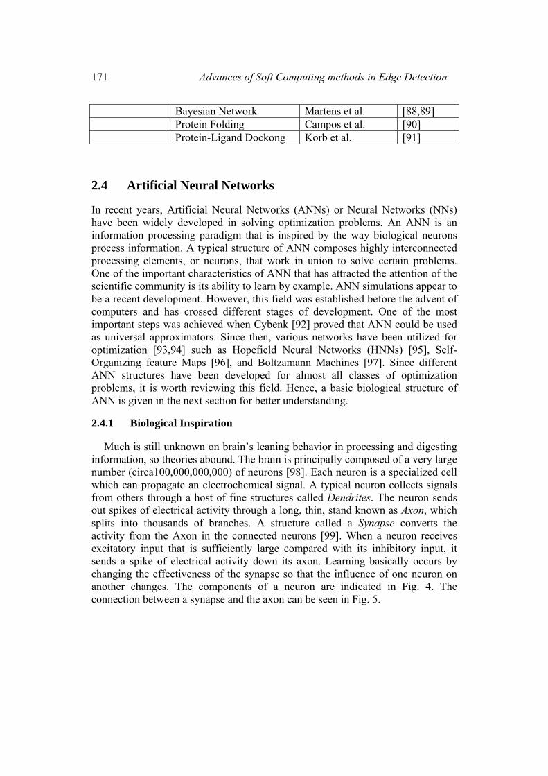
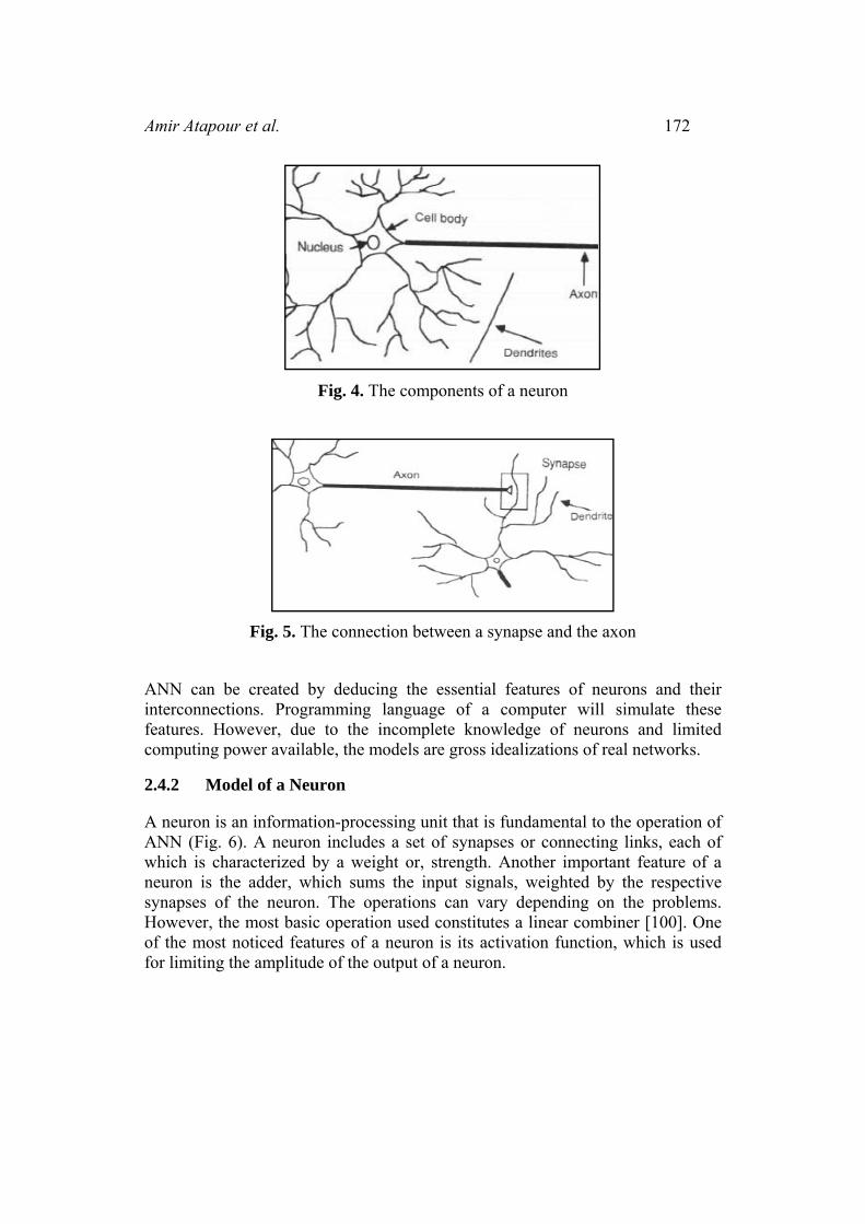
Much is still unknown on brain’s leaning behavior in processing and digesting information, so theories abound. The brain is principally composed of a very large number (circa100,000,000,000) of neurons [98]. Each neuron is a specialized cell which can propagate an electrochemical signal. A typical neuron collects signals from others through a host of fine structures called Dendrites. The neuron sends out spikes of electrical activity through a long, thin, stand known as Axon, which splits into thousands of branches. A structure called a Synapse converts the activity from the Axon in the connected neurons [99]. When a neuron receives excitatory input that is sufficiently large compared with its inhibitory input, it sends a spike of electrical activity down its axon. Learning basically occurs by changing the effectiveness of the synapse so that the influence of one neuron on another changes. The components of a neuron are indicated in Fig. 4. The connection between a synapse and the axon can be seen in Fig. 5.


Fig. 4. The components of a neuron

Fig. 5. The connection between a synapse and the axon

ANN can be created by deducing the essential features of neurons and their interconnections. Programming language of a computer will simulate these features. However, due to the incomplete knowledge of neurons and limited computing power available, the models are gross idealizations of real networks.

2.4.2 Model of a Neuron

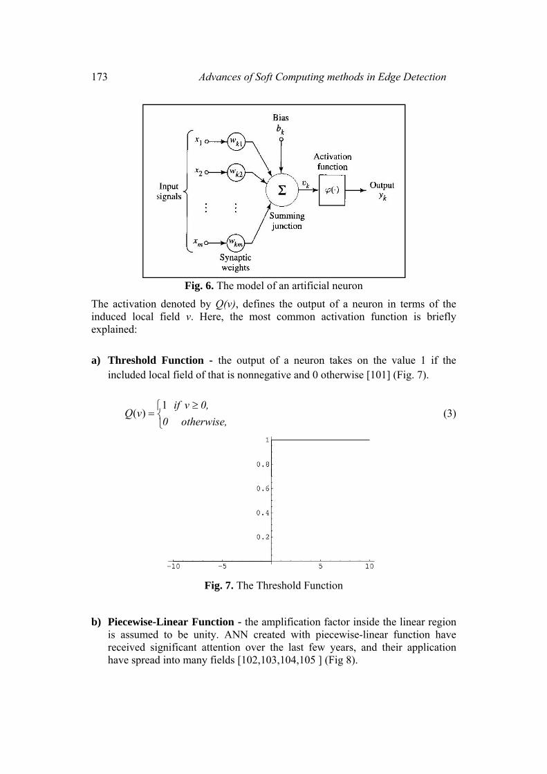
A neuron is an information-processing unit that is fundamental to the operation of ANN (Fig. 6). A neuron includes a set of synapses or connecting links, each of which is characterized by a weight or, strength. Another important feature of a neuron is the adder, which sums the input signals, weighted by the respective synapses of the neuron. The operations can vary depending on the problems. However, the most basic operation used constitutes a linear combiner [100]. One of the most noticed features of a neuron is its activation function, which is used for limiting the amplitude of the output of a neuron.


Fig. 6. The model of an artificial neuron

The activation denoted by Q(v), defines the output of a neuron in terms of the induced local field v. Here, the most common activation function is briefly explained:

a) Threshold Function - the output of a neuron takes on the value 1 if the

included local field of that is nonnegative and 0 otherwise [101] (Fig. 7).

⎩⎨⎧ ≥

=otherwise, 0

0,v if vQ

1)( (3)

Fig. 7. The Threshold Function

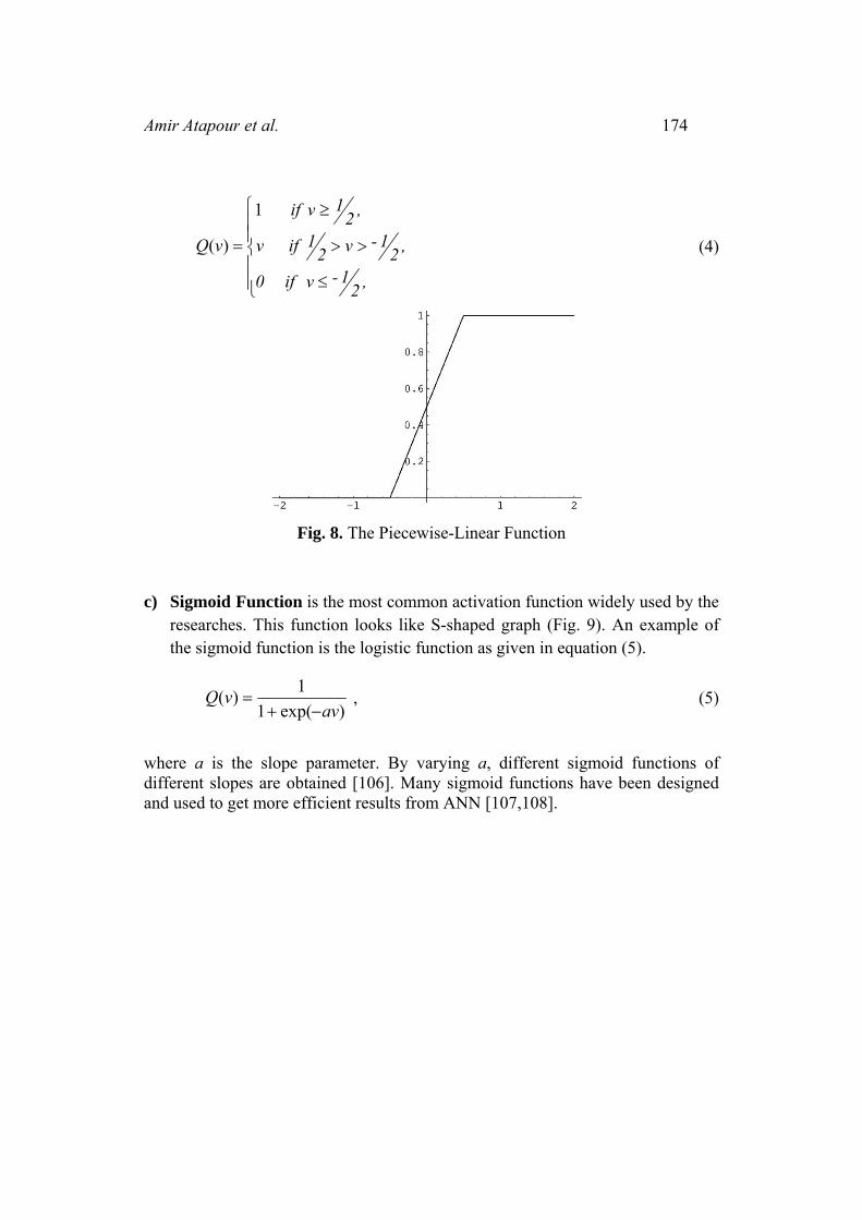
b) Piecewise-Linear Function - the amplification factor inside the linear region is assumed to be unity. ANN created with piecewise-linear function have received significant attention over the last few years, and their application have spread into many fields [102,103,104,105 ] (Fig 8).


⎪⎪⎩

⎪⎪⎨

⎧

≤

>>

≥

=

,21-v if 0

,21-v2

1 if v

,21v if

vQ

1

)( (4)

Fig. 8. The Piecewise-Linear Function

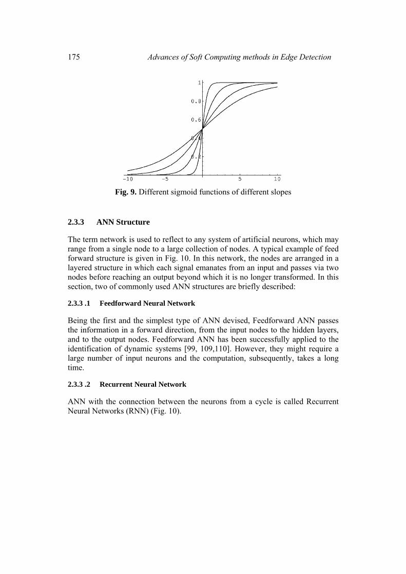
c) Sigmoid Function is the most common activation function widely used by the

researches. This function looks like S-shaped graph (Fig. 9). An example of the sigmoid function is the logistic function as given in equation (5).

)exp(11)(

avvQ

−+= , (5)

where a is the slope parameter. By varying a, different sigmoid functions of different slopes are obtained [106]. Many sigmoid functions have been designed and used to get more efficient results from ANN [107,108].


Fig. 9. Different sigmoid functions of different slopes

2.3.3 ANN Structure

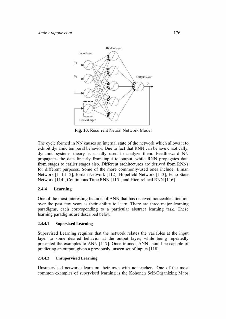
The term network is used to reflect to any system of artificial neurons, which may range from a single node to a large collection of nodes. A typical example of feed forward structure is given in Fig. 10. In this network, the nodes are arranged in a layered structure in which each signal emanates from an input and passes via two nodes before reaching an output beyond which it is no longer transformed. In this section, two of commonly used ANN structures are briefly described:

2.3.3 .1 Feedforward Neural Network

Being the first and the simplest type of ANN devised, Feedforward ANN passes the information in a forward direction, from the input nodes to the hidden layers, and to the output nodes. Feedforward ANN has been successfully applied to the identification of dynamic systems [99, 109,110]. However, they might require a large number of input neurons and the computation, subsequently, takes a long time.

2.3.3 .2 Recurrent Neural Network

ANN with the connection between the neurons from a cycle is called Recurrent Neural Networks (RNN) (Fig. 10).


Fig. 10. Recurrent Neural Network Model

The cycle formed in NN causes an internal state of the network which allows it to exhibit dynamic temporal behavior. Due to fact that RNN can behave chaotically, dynamic systems theory is usually used to analyze them. Feedforward NN propagates the data linearly from input to output, while RNN propagates data from stages to earlier stages also. Different architectures are derived from RNNs for different purposes. Some of the more commonly-used ones include: Elman Network [111,112], Jordan Network [112], Hopefield Network [113], Echo State Network [114], Continuous Time RNN [115], and Hierarchical RNN [116].

2.4.4 Learning

One of the most interesting features of ANN that has received noticeable attention over the past few years is their ability to learn. There are three major learning paradigms, each corresponding to a particular abstract learning task. These learning paradigms are described below.

2.4.4.1 Supervised Learning

Supervised Learning requires that the network relates the variables at the input layer to some desired behavior at the output layer, while being repeatedly presented the examples to ANN [117]. Once trained, ANN should be capable of predicting an output, given a previously unseen set of inputs [118].

2.4.4.2 Unsupervised Learning

Unsupervised networks learn on their own with no teachers. One of the most common examples of supervised learning is the Kohonen Self-Organizing Maps


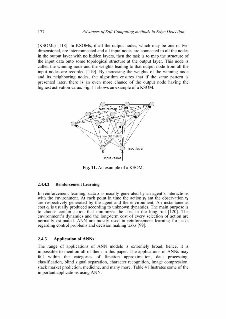
(KSOMs) [118]. In KSOMs, if all the output nodes, which may be one or two dimensional, are interconnected and all input nodes are connected to all the nodes in the output layer with no hidden layers, then the task is to map the structure of the input data onto some topological structure at the output layer. This node is called the winning node and the weights leading to that output node from all the input nodes are recorded [119]. By increasing the weights of the winning node and its neighboring nodes, the algorithm ensures that if the same pattern is presented later, there is an even more chance of the output node having the highest activation value. Fig. 11 shows an example of a KSOM.

Fig. 11. An example of a KSOM.

2.4.4.3 Reinforcement Learning

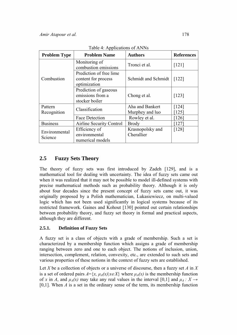
In reinforcement learning, data x is usually generated by an agent’s interactions with the environment. At each point in time the action ant the observation are respectively generated by the agent and the environment. An instantaneous cost is usually produced according to unknown dynamics. The main purpose is to choose certain action that minimizes the cost in the long run [120]. The environment’s dynamics and the long-term cost of every selection of action are normally estimated. ANN are mostly used in reinforcement learning for tasks regarding control problems and decision making tasks [99]. 2.4.5 Application of ANNs The range of applications of ANN models is extremely broad; hence, it is impossible to mention all of them in this paper. The applications of ANNs may fall within the categories of function approximation, data processing, classification, blind signal separation, character recognition, image compression, stack market prediction, medicine, and many more. Table 4 illustrates some of the important applications using ANN.


Table 4: Applications of ANNs Problem Type Problem Name Authors References

Combustion

Monitoring of combustion emissions Tronci et al. [121]

Prediction of free lime content for process optimization

Schmidt and Schmidt [122]

Prediction of gaseous emissions from a stocker boiler

Chong et al. [123]

Pattern Recognition

Classification Aha and Bankert Murphey and luo

[124] [125]

Face Detection Rowley et al. [126] Business Airline Security Control Brody [127]

Environmental Science

Efficiency of environmental numerical models

Krasnopolsky and Cherallier

[128]

2.5 Fuzzy Sets Theory

The theory of fuzzy sets was first introduced by Zadeh [129], and is a mathematical tool for dealing with uncertainty. The idea of fuzzy sets came out when it was realized that it may not be possible to model ill-defined systems with precise mathematical methods such as probability theory. Although it is only about four decades since the present concept of fuzzy sets came out, it was originally proposed by a Polish mathematician, Lukasiewiecz, on multi-valued logic which has not been used significantly in logical systems because of its restricted framework. Gaines and Kohout [130] pointed out certain relationships between probability theory, and fuzzy set theory in formal and practical aspects, although they are different.

2.5.1. Definition of Fuzzy Sets

A fuzzy set is a class of objects with a grade of membership. Such a set is characterized by a membership function which assigns a grade of membership ranging between zero and one to each object. The notions of inclusion, union, intersection, complement, relation, convexity, etc., are extended to such sets and various properties of these notions in the context of fuzzy sets are established.

Let X be a collection of objects or a universe of discourse, then a fuzzy set A in X is a set of ordered pairs A={x, µA(x)|x∈X} where µA(x) is the membership function of x in A, and µA(x) may take any real values in the interval [0,1] and µA : X → [0,1]. When A is a set in the ordinary sense of the term, its membership function


can take only two values 0 and 1, with µA(x) = 1 or 0 accordingly, as x does or does not belong to A.

2.5.2 Membership Function

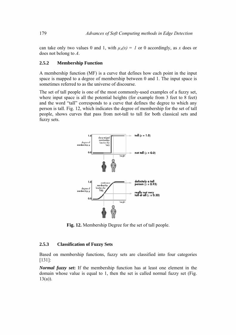
A membership function (MF) is a curve that defines how each point in the input space is mapped to a degree of membership between 0 and 1. The input space is sometimes referred to as the universe of discourse.

The set of tall people is one of the most commonly-used examples of a fuzzy set, where input space is all the potential heights (for example from 3 feet to 8 feet) and the word “tall” corresponds to a curve that defines the degree to which any person is tall. Fig. 12, which indicates the degree of membership for the set of tall people, shows curves that pass from not-tall to tall for both classical sets and fuzzy sets.

Fig. 12. Membership Degree for the set of tall people.

2.5.3 Classification of Fuzzy Sets

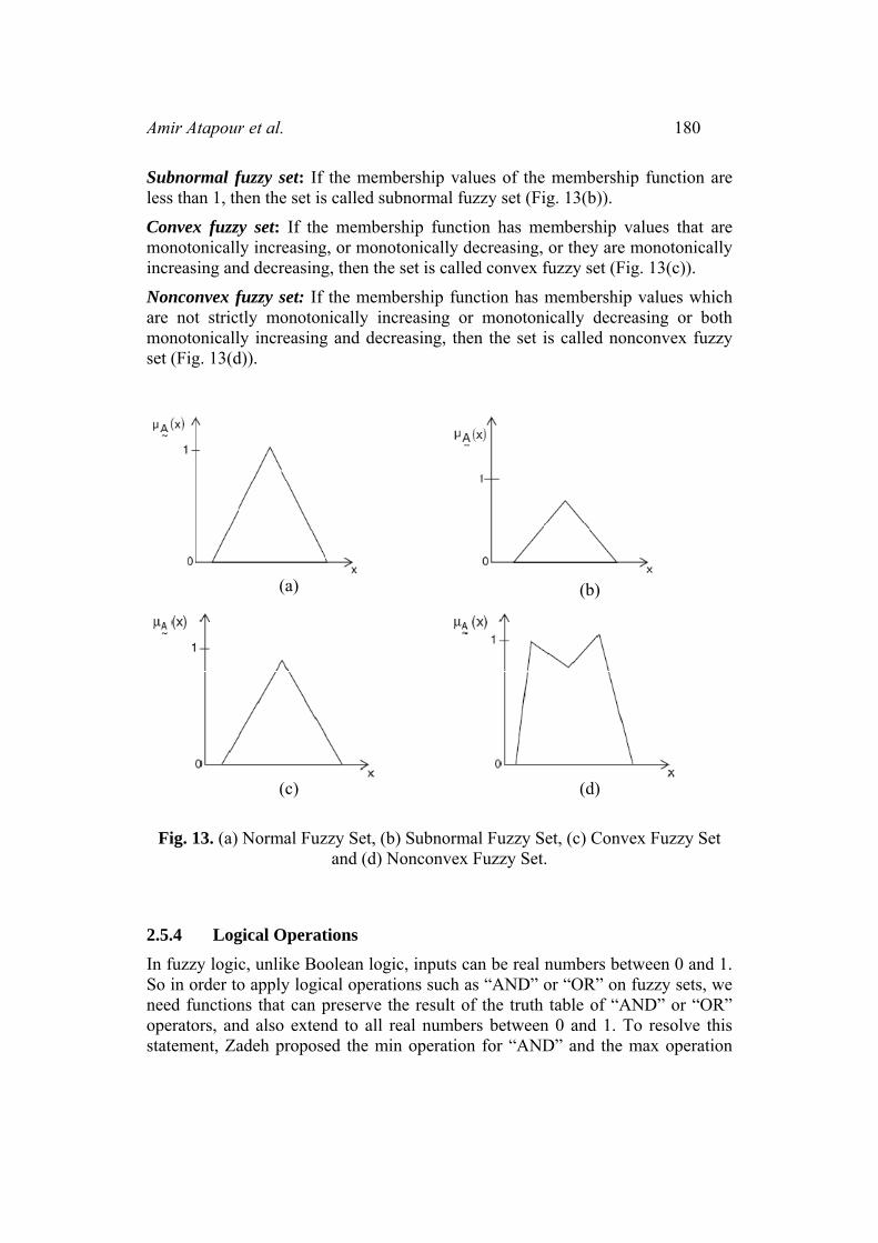
Based on membership functions, fuzzy sets are classified into four categories [131]:

Normal fuzzy set: If the membership function has at least one element in the domain whose value is equal to 1, then the set is called normal fuzzy set (Fig. 13(a)).


Subnormal fuzzy set: If the membership values of the membership function are less than 1, then the set is called subnormal fuzzy set (Fig. 13(b)).

Convex fuzzy set: If the membership function has membership values that are monotonically increasing, or monotonically decreasing, or they are monotonically increasing and decreasing, then the set is called convex fuzzy set (Fig. 13(c)).

Nonconvex fuzzy set: If the membership function has membership values which are not strictly monotonically increasing or monotonically decreasing or both monotonically increasing and decreasing, then the set is called nonconvex fuzzy set (Fig. 13(d)).

(a)

(b)

(c)

(d)

Fig. 13. (a) Normal Fuzzy Set, (b) Subnormal Fuzzy Set, (c) Convex Fuzzy Set and (d) Nonconvex Fuzzy Set.

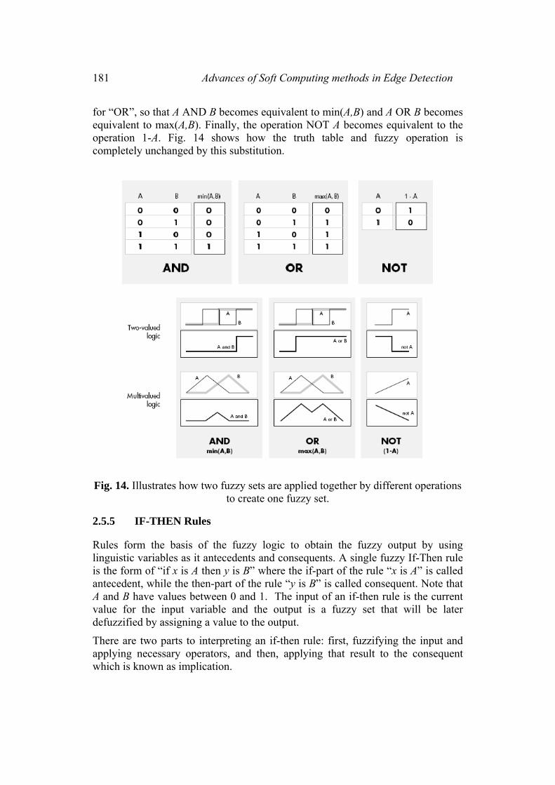
2.5.4 Logical Operations In fuzzy logic, unlike Boolean logic, inputs can be real numbers between 0 and 1. So in order to apply logical operations such as “AND” or “OR” on fuzzy sets, we need functions that can preserve the result of the truth table of “AND” or “OR” operators, and also extend to all real numbers between 0 and 1. To resolve this statement, Zadeh proposed the min operation for “AND” and the max operation


for “OR”, so that A AND B becomes equivalent to min(A,B) and A OR B becomes equivalent to max(A,B). Finally, the operation NOT A becomes equivalent to the operation 1-A. Fig. 14 shows how the truth table and fuzzy operation is completely unchanged by this substitution.

Fig. 14. Illustrates how two fuzzy sets are applied together by different operations to create one fuzzy set.

2.5.5 IF-THEN Rules

Rules form the basis of the fuzzy logic to obtain the fuzzy output by using linguistic variables as it antecedents and consequents. A single fuzzy If-Then rule is the form of “if x is A then y is B” where the if-part of the rule “x is A” is called antecedent, while the then-part of the rule “y is B” is called consequent. Note that A and B have values between 0 and 1. The input of an if-then rule is the current value for the input variable and the output is a fuzzy set that will be later defuzzified by assigning a value to the output.

There are two parts to interpreting an if-then rule: first, fuzzifying the input and applying necessary operators, and then, applying that result to the consequent which is known as implication.


2.5.6 Fuzzy Inference Systems

Fuzzy inference systems (FISs) [131], also known as fuzzy rule-based systems, are the process of formulating the mapping from a given input to an output using fuzzy logic. This process involves all the steps described before, membership functions, fuzzy logic operators, and if-then rules.

The two most important types of fuzzy inference are Mamdani’s method [132] and Sugeno’s method [133]. Mamdani inference method, introduced by Mamdani and Assilian, is the most commonly-used in various areas. The other well-known method, Sugeno method or Takagi-Sugeno-Kang method was introduced by Sugeno. These two types are different in the way outputs are determined.

2.5.6.1 Mamdani’s Fuzzy Interface

Mamdani’s fuzzy inference method is the most commonly-seen fuzzy methodology. This method was among the first control systems built using fuzzy set theory. It was proposed in 1975 as an attempt to control a steam engine and boiler combination by synthesizing a set of linguistic control rules, obtained from experienced human operators. His effort was based on Zadeh’s paper on fuzzy algorithms for complex systems and decision processes [134].

In order to compute the output of a given FIS from the inputs, these five steps should be done:

Fuzzifying Inputs: The first step is determining the degree of membership of each input using membership functions.

Applying Fuzzy Operators: After inputs have been fuzzified, if the antecedent of a rule has more than one part, the fuzzy operator is applied to obtain the result. The result will then be given to the output function. So the input is two or more membership values from fuzzified inputs and the output is a truth value.

Applying Implication Method: Implication method is the process of determining the output of each fuzzy rule’s consequent. Before applying the implication method, we must take care of the rule’s weight which is a number between 0 and 1. Generally this weight is 1 and so it has no effect on the implication process. The input of implication is a single number given by the antecedent, and the output is a fuzzy set.

Aggregating All Outputs: At this stage, all fuzzy sets that represent the outputs of each rule, are combined into a single fuzzy set. The input is output functions returned by the implication process of each rule and the output is one fuzzy set for each output variable. There are different methods to apply the aggregation such as maximum, probabilistic or, and sum.

Defuzzifying: Although fuzziness helps during the previous steps, the desired final output is a single number. To do so the output fuzzy set of aggregation


process must be converted into a single number. The most common method is the centroid calculation.

2.5.5 Applications of Fuzzy Sets

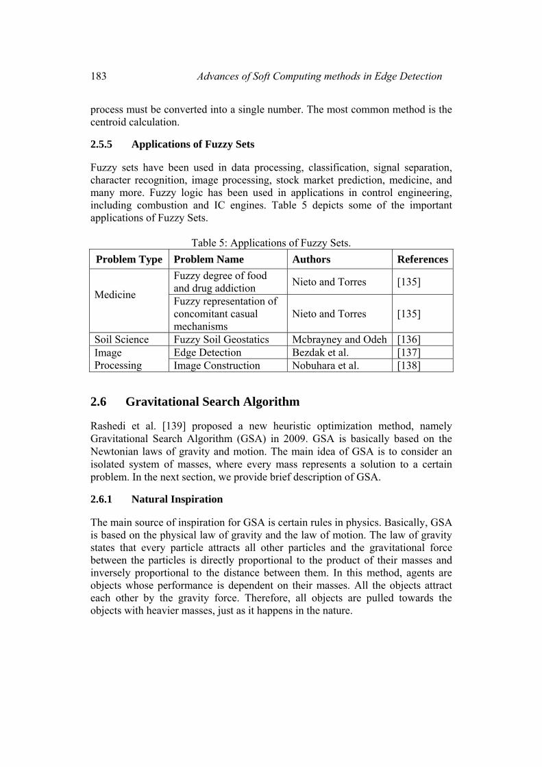
Fuzzy sets have been used in data processing, classification, signal separation, character recognition, image processing, stock market prediction, medicine, and many more. Fuzzy logic has been used in applications in control engineering, including combustion and IC engines. Table 5 depicts some of the important applications of Fuzzy Sets.

Table 5: Applications of Fuzzy Sets. Problem Type Problem Name Authors References

Medicine

Fuzzy degree of food and drug addiction Nieto and Torres [135]

Fuzzy representation of concomitant casual mechanisms

Nieto and Torres [135]

Soil Science Fuzzy Soil Geostatics Mcbrayney and Odeh [136] Image Processing

Edge Detection Bezdak et al. [137] Image Construction Nobuhara et al. [138]

2.6 Gravitational Search Algorithm

Rashedi et al. [139] proposed a new heuristic optimization method, namely Gravitational Search Algorithm (GSA) in 2009. GSA is basically based on the Newtonian laws of gravity and motion. The main idea of GSA is to consider an isolated system of masses, where every mass represents a solution to a certain problem. In the next section, we provide brief description of GSA.

2.6.1 Natural Inspiration

The main source of inspiration for GSA is certain rules in physics. Basically, GSA is based on the physical law of gravity and the law of motion. The law of gravity states that every particle attracts all other particles and the gravitational force between the particles is directly proportional to the product of their masses and inversely proportional to the distance between them. In this method, agents are objects whose performance is dependent on their masses. All the objects attract each other by the gravity force. Therefore, all objects are pulled towards the objects with heavier masses, just as it happens in the nature.


2.6.2 How GSA Works

Suppose there is a system with N agents, the position of every agent is a point in the search space which represents a solution to the problem. The position of the ith agent is defined as follows:

),...,,...,( 1 ni

diii xxxX = Ni ,...,2,1= (6)

Where n is the dimension of the problem, and is the position of the ith agent in the dth dimension.

At the starting point of the solution the agents are situated randomly. At the specific time ‘t’ a gravitational force from mass ‘j’ acts on mass ‘i’, and is defined as follows:

))()(()(

)()()()( txtx

tRtMtM

tGtF di

dj

ij

ajpidij −

+×

=ε , (7)

Where,

is the mass of the object i,

is the mass of the object j,

G(t) is the gravitational constant at time t,

(t) is the Euclidian distance between the two objects i and j, and

ε is a small constant.

The gravitational constant, G, which is initialized randomly, decreases by time to control the search accuracy.

In other words, G is a function of the initial value (G0) and time (t):

),()( 0 tGGtG = (8)

The total force acting on agent i in the dimension d is calculated as follows:

(t)Frand(t)Fikbest,jj

dijj

di ∑

≠∈

= (9)

Where is a random number in the interval [0,1] and is used to give a randomized characteristics to the search.

According to the law of motion, the acceleration of the agent i, at time t, in the dth dimension is directly proportional to the force acting on that agent, and inversely proportional to the mass of the agent:


)()()(

tMtFta

ii

did

i = (10)

Furthermore, the next velocity of an agent is a function of its current velocity added to its current acceleration. Therefore, the next position and the next velocity of an agent can be calculated as follows:

)()()1( tatvrandtv di

dii

di +⋅=+ , (11)

)1()()1( ++=+ tvtxtx di

di

di , (12)

Where (t) is the velocity of the agent in the dth dimension at time t, and is a random number in the interval [0,1].

The masses of the agents are calculated using fitness evaluation. The heavier the mass of an agent, the more efficient is that agent, regarding the solution it represents. It is notable that as the law of gravity and the law of motion imply, a heavy mass has a higher attraction power and moves more slowly.

The masses are updated as follows:

)()()()()(tworsttbesttworsttfittm i

i −−

= (13)

Where (t) represents the fitness value of the agent i at time t, and the best(t) and worst(t) in the population respectively indicate the strongest and the weakest agent according to their fitness route. For a maximization problem best(t) and worst(t) can be defined as follows:

)(max)(},..,1{

tfittworst jNj∈= (14)

)(min)(},..,1{

tfittbest jNj∈= (15)

The updated masses, obtained from the equation (13) must be normalized using the following equation:

∑=

= N

jj

ii

tm

tmtM

1)(

)()( (16)

At the beginning of the system establishment, every agent is located at a certain point of the search space which represents a solution to the problem at every unit of time. The agents are evaluated and their next positions are calculated using the equations (11) and equation (12). Other parameters of the algorithm like the gravitational constant and masses are also calculated using equation (8), equation (13), and equation (16). These equations are updated at every unit of time. The


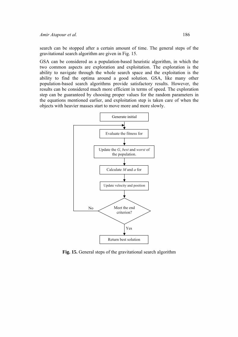
search can be stopped after a certain amount of time. The general steps of the gravitational search algorithm are given in Fig. 15.

GSA can be considered as a population-based heuristic algorithm, in which the two common aspects are exploration and exploitation. The exploration is the ability to navigate through the whole search space and the exploitation is the ability to find the optima around a good solution. GSA, like many other population-based search algorithms provide satisfactory results. However, the results can be considered much more efficient in terms of speed. The exploration step can be guaranteed by choosing proper values for the random parameters in the equations mentioned earlier, and exploitation step is taken care of when the objects with heavier masses start to move more and more slowly.

Fig. 15. General steps of the gravitational search algorithm

Generate initial

Evaluate the fitness for

Update the G, best and worst of the population.

Calculate M and a for

Update velocity and position

Meet the end criterion?

Return best solution

Yes

No


3 Results and Discussion

In this section, we provide Soft Computing application on edge detection, which is an important feature in image processing and machine vision.

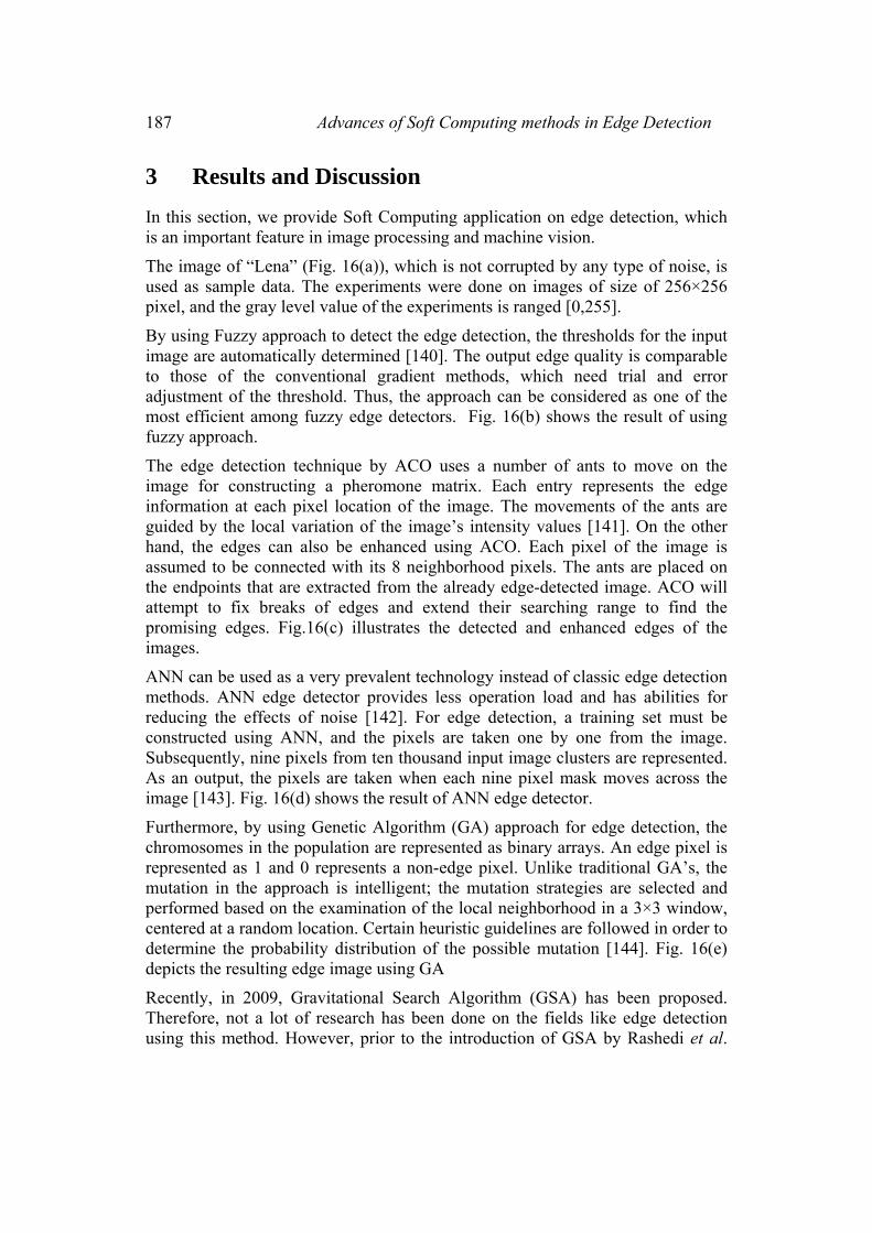
The image of “Lena” (Fig. 16(a)), which is not corrupted by any type of noise, is used as sample data. The experiments were done on images of size of 256×256 pixel, and the gray level value of the experiments is ranged [0,255].

By using Fuzzy approach to detect the edge detection, the thresholds for the input image are automatically determined [140]. The output edge quality is comparable to those of the conventional gradient methods, which need trial and error adjustment of the threshold. Thus, the approach can be considered as one of the most efficient among fuzzy edge detectors. Fig. 16(b) shows the result of using fuzzy approach.

The edge detection technique by ACO uses a number of ants to move on the image for constructing a pheromone matrix. Each entry represents the edge information at each pixel location of the image. The movements of the ants are guided by the local variation of the image’s intensity values [141]. On the other hand, the edges can also be enhanced using ACO. Each pixel of the image is assumed to be connected with its 8 neighborhood pixels. The ants are placed on the endpoints that are extracted from the already edge-detected image. ACO will attempt to fix breaks of edges and extend their searching range to find the promising edges. Fig.16(c) illustrates the detected and enhanced edges of the images.

ANN can be used as a very prevalent technology instead of classic edge detection methods. ANN edge detector provides less operation load and has abilities for reducing the effects of noise [142]. For edge detection, a training set must be constructed using ANN, and the pixels are taken one by one from the image. Subsequently, nine pixels from ten thousand input image clusters are represented. As an output, the pixels are taken when each nine pixel mask moves across the image [143]. Fig. 16(d) shows the result of ANN edge detector.

Furthermore, by using Genetic Algorithm (GA) approach for edge detection, the chromosomes in the population are represented as binary arrays. An edge pixel is represented as 1 and 0 represents a non-edge pixel. Unlike traditional GA’s, the mutation in the approach is intelligent; the mutation strategies are selected and performed based on the examination of the local neighborhood in a 3×3 window, centered at a random location. Certain heuristic guidelines are followed in order to determine the probability distribution of the possible mutation [144]. Fig. 16(e) depicts the resulting edge image using GA

Recently, in 2009, Gravitational Search Algorithm (GSA) has been proposed. Therefore, not a lot of research has been done on the fields like edge detection using this method. However, prior to the introduction of GSA by Rashedi et al.


[139], some studies were done based on the theory of universal gravity [145]. The edge detection approach used here is also based upon the idea of universal gravity which is extremely similar to the GSA, with a slight difference in the way the distance of the agents is used in the equation (7). To construct an edge detector, every pixel is assumed to be an object, which has some relationship with other pixels within its neighborhood through gravitational forces. For each pixel, the magnitude and the direction of the vector of the sum of all the gravitational forces the pixel exerts on its neighborhood, conveys the vitally important information about an edge structure. Fig. 16(f) shows the efficiency of GSA edge detection method.

(a)

(b)

(c)

(d)

(e)

(f)

Fig. 16. The original image, (b) Fuzzy edge detector applied to the image, (c) ACO-based edge detector applied to the image (d) Neural Network edge detector

applied to the image, (e) GA-based edge detector applied to the image, and (f) Universal Gravity edge detector applied to the image.


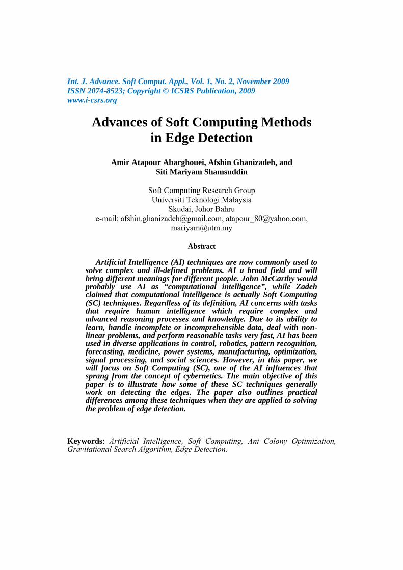
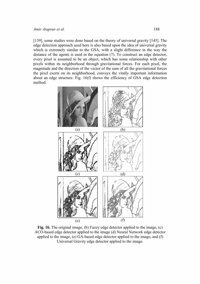
The methods mentioned above have certain advantages and disadvantages that separate them from each other in terms of performance. Fig. 17, and Table 6. Indicate some of the advantages of the edge detection methods. The disadvantages of the same methods are reviewed in Fig. 18, and Table 7.

Fig. 17. Advantages of the discussed Methods: (a) Universal Gravity edge detector, (b) Fuzzy edge detector, (c) ACO-based edge detector (d) Neural

Network edge detector, and (e) GA-based edge detector.

(a)

(b)

(c)

(d)

(e)


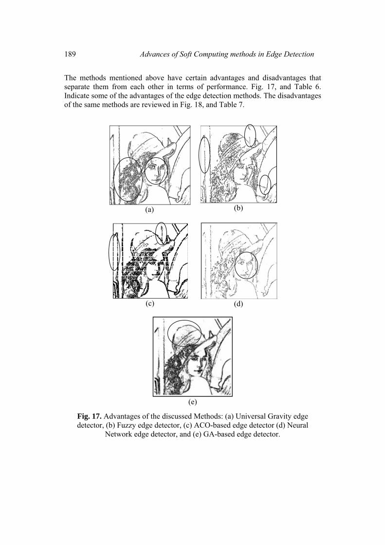
Table 6: Advantages of the discussed methods. Method Advantages

Gravitational Search Algorithm

• Using this method, the edges are selected more smoothly in the selected features shown in Fig. 17(a). For instance, the facial features are much closer to the original image.

• The method works acceptably well on noisy images. Fuzzy Sets Theory

• Unlike many other edge detectors, the selected features in Fig. 17(b) are correctly considered as edges.

• This method does not include a lot of parameter setting. • Fuzzy edge detectors are relatively faster than other

methods. • Many of the Fuzzy edge detection methods work well on

noisy images. Ant Colony Optimization

• Unlike many other edge detectors, the selected features in Fig. 17(c) are correctly considered as edges.

• The ACO-based method can be used as a great edge-enhancement method for the already detected edges.

Artificial Neural Network

• In this method, the neural networks can be trained using specific patterns, in order to achieve more accurate edges.

• Using this method, the edges are selected more smoothly in the selected features shown in Fig. 17(d). For instance, the facial features are much closer to the original image.

Genetic Algorithm

• Unlike many other edge detectors, the selected features in Fig. 17(e) are correctly considered as edges.


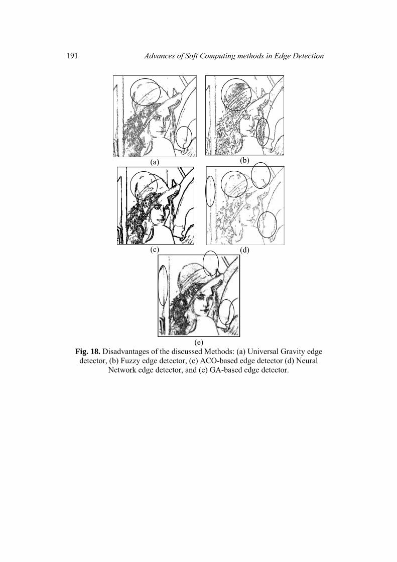
Fig. 18. Disadvantages of the discussed Methods: (a) Universal Gravity edge detector, (b) Fuzzy edge detector, (c) ACO-based edge detector (d) Neural

Network edge detector, and (e) GA-based edge detector.

(a)

(b)

(c)

(d)

(e)


Table 7: Disadvantages of the discussed methods. Method Disadvantages

Gravitational Search Algorithm

• Many parameters have to be set correctly, in order to achieve the best possible edge detector for every image (including mask, threshold, etc.).

• Unlike many other edge detectors, the selected features shown in Fig. 18(a) are not considered as edges by mistake.

Fuzzy Sets Theory

• Unlike many other edge detectors, the selected features shown in Fig. 18(b) are not considered as edges by mistake.

Ant Colony Optimization

• Many parameters have to be set correctly, in order to achieve the best possible edge detector for every image (including the number of iterations, the number of ants, etc.).

• Unlike many other edge detectors, the selected features shown in Fig. 18(c) are not considered as edges by mistake.

• This method works relatively slow, in comparison with other edge detection methods.

Artificial Neural Network

• As shown in the selected features in Fig. 18(d), many of the edges that are usually found by other edge detection methods are not considered as edges.

Genetic Algorithm

• Many parameters have to be set correctly, in order to achieve the best possible edge detector for every image (including the number of iterations, the number of individuals in the selected population, etc.).

• Unlike many other edge detectors, the selected features shown in Fig. 18(e) are not considered as edges by mistake.

• This method works relatively slow, in comparison with other edge detection methods, and can lead to unacceptable results depending on the number of iterations.

4 Conclusion & Future Work In this paper, a brief description of five major Soft Computing techniques is given; Fuzzy sets, Artificial Neural Networks, Ant Colony Optimization, Genetic Algorithm, and Gravitational Search Algorithm, and the advances made in their structure and their applications, especially in the field of edge detection [140,141,142,143,144,145] were discussed.

All the techniques were compared with each other by applying them on edge detection, which is of the utmost importance in the field of image processing. The performances of the techniques were compared by presenting the results of each technique, when used on the same problem in the same conditions. This paper


presents a survey on soft computing methods particularly for edge detection. All of these techniques have relative advantages and disadvantages and there are no rules as to when a particular technique is more or less suitable for a new application; hence Free Lunch Theorem should be applied.

Although an incredible amount of research has been done on using soft computing methods in edge detection, many of the vast and newly-proposed methods still have a lot of potential for improvement. There are a lot of possible hybrid methods that the researchers can explore. Neuro-fuzzy, which is a combination of neural networks and fuzzy sets theory, can be an excellent example of a highly advantageous method for edge detection. ACO can act as an edge enhancement method, and is predicted to give astonishing result when applied on edges detected using a fuzzy method.

There are many other optimization methods that could be possible to integrate with ANN, in terms of training or as a hybrid method, such as Differential Evolution [146], Bacteria Foraging [147], Artificial Fish Swarm Algorithm [148], and others. Future research can hopefully end in new methods with better results.

ACKNOWLEDGEMENTS.

This work is supported by Universiti Teknologi Malaysia, Skudai Johor Bahru MALAYSIA. Authors would like to thank Soft Computing Research Group (SCRG) for their moral support and incisive comments to improve this article.

References [1] J.H. Holland, Adaptation in Natural and Artificial Systems, Univ. of

Michigan Press, Ann Arbor, Mich., (1975). [2] M. Huanga, C.J. Aine, S. Supek, E. Best, D. Rankena, and E.R. Flynn,

“Multi-start downhill simplex method for spatio-temporal source localization in magneto encephalography”, Electroencephalography and clinical Neurophysiology, 108, (1998), pp. 32–44.

[3] R.L. Haupt, and S.E. Haupt, Practical Genetic Algorithm, John Wiley & Sons, Inc., (2004).

[4] S.N. Sivanandam, and S.N.Deepa, Introduction to Genetic Algorithms, Springer, (2008).

[5] M. Srinivas, and L.M. Patnaik, “Genetic Algorithm: A Survey”, IEEE Computer Society, Vol.27, No.6, (1994), pp. 17 – 26.

[6] Ch. Prins, “Two memetic algorithms for heterogeneous fleet vehicle routing problems”, Engineering Applications of Artificial Intelligence, 22, (2009), pp. 916–928.

[7] F. Zha, S. Li, J. Sun, and D. Mei, “Genetic algorithm for the one-commodity pickup-and-delivery traveling salesman problem”, Computers & Industrial Engineering, 56, (2009), pp. 1642–1648.


[8] K. Gallacher, and M. Sambridge, “Genetic Algorithm: A Powerful Tool for Large-Scale Nonlinear Optimization Problems”, Computers & Industrial Engineering, 56, (2009), pp. 1642–1648.

[9] G. Renner, and A. Ekart, “Genetic algorithms in computer aided design”, Computer-Aided Design, 35, (2003), pp. 709–726.

[10] X.Hu, and E. Di Paolo, “An efficient genetic algorithm with uniform crossover for air traffic control”, Computers & Operations Research, 36, (2009), pp. 245–259.

[11] L.J. Eshelman, R. Caruna, and J.D. Schaffer, “Biases in the crossover landscape, in: J.D. Schaffer (Ed.)”, Proceedings of the Third International Conference on Genetic Algorithms, (1989), pp. 10–19.

[12] B. Lazzerini, and F. Marcelloni, “A genetic algorithm for generating optimal assembly plans”, Artificial Intelligence in Engineering, 14, (2000), pp. 319–329.

[13] A.T. Haghighat, K. Faez, M. Dehghan, A. Mowlaei, and Y. Ghahremani, “GA-Based Heuristic Algorithms for QoS Based Multicast Routing”, Knowledge-Based Systems, 16, (2003), pp. 305–312.

[14] J.D. Schaffer, “Multiple objective optimization with vector evaluated genetic algorithms”, Genetic Algorithms Appl: Proc First Int Conf Genetic Algorithms, (1985), pp.93–100.

[15] E. Cantu-Paz “A survey on parallel genetic algorithms”, ILLIGAL report 97003, University of Illinois at Urbana-Champain, (1997).

[16] DE. Goldberg, Genetic algorithms in search optimization, and machine learning, Addison-Wesley, (1989).

[17] D. Beasley, D.R. Bull, and R.R. Martin, “A sequential niche technique for multi-modal function optimization”, Evolutionary Computing,Vol.1, No.2, (1993), pp.101–25.

[18] T. Back, Evolutionary Algorithms in Theory and Practice, Oxford University Press, (1996).

[19] J. Horn, N. Nafpliotis, and DE. Goldberg, “A niched Pareto genetic algorithm for multiobjective optimization”, Proc First IEEE Conf Evolutionary Computing, (1994), pp. 82–7.

[20] S. Mahfoud, “Niching methods for genetic algorithms”, ILLIGAL report 95001, University of Illinois at Urbana-Champaign, (1995).

[21] C.K. Oei, DE. Goldberg, and SJ. Chang, “Tournament selection, niching and the preservation of diversity”, ILLIGAL report 91011, University of Illinois at Urbana-Champaign, (1991).

[22] X. Yin, and N.Germay, “A fast genetic algorithm with sharing scheme using cluster analysis methods in multimodal function optimization”, Artificial neural nets and genetic algorithms, (1993). pp. 450–457.

[23] DE. Goldberg, “Genetic algorithms as a computational theory of conceptual design”, Appl Artif Intell Engng, (1991), pp. 3–16.


[24] P.J. Bentley, and J.P. Wakefield, “Conceptual evolutionary design by a genetic algorithm”, Engng Des Automation, Vol.3 No.2, (1997), pp. 119–131.

[25] K. Rasheed, H. Hirsh, and A.Gelsey, “A genetic algorithm for continuous design space search”, Artif Intell Engng, 11, (1997), pp.295–305.

[26] J. Gero, and V. Kazakov, “Adaptive enlargement of state spaces in evolutionary designing”, Artif Intell Engng Des, Anal Manufact, 14, (2000), pp. 31–38.

[27] A. Markus, G. Renner, and J. Vancza, “interpolation with genetic algorithms”, Shape Modeling Appl, (1997), pp.47–54.

[28] A. Limaiem, A. Nassef, and HA. El-Maraghy, “Data fitting using dual kriging and genetic algorithms”, Ann CIRP, Vol. 45, No. 1, (1996), pp.129–134.

[29] M. Manela, N. Thornhill, and JA.Campbell, “Fitting spline functions to noisy data using a genetic algorithm”, Proc Fifth Int Conf Genetic Algorithms, (1993), pp.549–553.

[30] CL. Karr, B. Weck, DL. Massart, and P. Vankeerberghen, “Least median squares curve fitting using a genetic algorithm”, Engng Appl Artif Intell, Vol. 8 No.2, (1995), pp. 177–189.

[31] JJ. Jacq, and C. Roux, “Registration of 3D images by genetic optimization”, Pattern Recognition, Vol. 16, No.8, (1995), pp. 823–856.

[32] SM. Yamany, MN. Ahmed, and AA. Farag, “A new genetic-based technique for matching 3D curves and surfaces”, Pattern Recognition, 32, (1999), pp. 1817–20.

[33] A. Kunjur, and S. Krishnamurty “Genetic algorithms in mechanism synthesis”, Fourth Applied Mechanisms and Robotics Conference, (1995).

[34] J.K. Parker, A.R. Khoogar, and DE. Goldberg “Inverse kinematics of redundant robots using genetic algorithms”, IEEE Int Conf Robotics Automation, (1989), pp.271–276.

[35] KA. Buckley, SH. Hopkins, and BCH. Turton, “Solution of inverse kinematics problems of a highly kinematially redundant manipulator using genetic algorithms”, Genetic Algorithms Engng Syst: Innovations Appl, (1997), pp.264–9.

[36] AS. Rana, and AMS. Zalzala, “An evolutionary algorithm for collision free motion planning of multi-arm robots”, Genetic Algorithms Engng Syst: Innovations Appl, (1995), pp.123–30.

[37] F. Menczer, and R. K. Belew, “Evolving sensors in eiivironments of controlled complexity”, Proceedings of the Fourth International Workshop on Synthesis and Simulation of Living systems, (1994), pp.210-221.

[38] N. Jakobi, “Harnessing morphogenesis”, International Conference on Information Processing in Cells and Tissues, Liverpool, UK. (1995).

[39] J. Bala, J.Huang, H. Vafaie, K. A. De Jong, and H. Wechsler, “Hybrid learning using genetic algorithms and decision trees for pattern


classification”, Proceedings of the 14'h International Joint Conference on Artificial Intelligence, (1995).

[40] E. A. Roache, K. A. Hickok, K. F. Loje, M. W. Hunt, and J. Grefenstette, “Genetic algorithms for expert system validation”, Proceedings of Western Multiconference, (1995).

[41] R.R. Hightower, S. Forrest, and A.S. Parelson, “The evolution of emergent organization in immune system gene libraries”, In L. J. Eshelman (Ed.) Proceedings of the Sixth International Conference on Genetic Algorithms, (1995), pp. 344-350.

[42] R. J. Parsons, S. Forrest, and C. Burks, “Genetic operators for the DNA fragment-assembly problem”, Machine Learning, 21(1/2), (1995), pp.11-33.

[43] J. Kennedy, and R. Eberhart, “Particle Swarm Optimization”, IEEE International Conference on Neural Networks (Perth, Australia), IEEE Service Center, Piscataway, (1995), pp. 1942-1948.

[44] M. Dorigo, “Optimization, learning and natural algorithms”, Ph.D. Thesis, Dipartimento di Elettronica, Politecnico di Milano, Italy, (1992).

[45] M. Dorigo, V. Maniezzo, “Ant Colony Positive feedback as a search strategy”, Tech. Report 91-016, Dipartimento di Elettronica, Politecnico di Milano, Italy, (1991).

[46] M. Dorigo, V. Maniezzo, and A. Colorni, “Ant system: optimization by a colony of cooperating agents”, IEEE Trans. Systems, Man, Cybernet, Part B 26 (1) , (1996), pp. 29–41.

[47] P.-P. Grassé, Les Insectes Dans Leur Univers, Paris, France: Ed. du Palais de la découverte, (1946).

[48] P.-P. Grassé, “La reconstruction du nid et les coordinations interindividuelles chez Bellicositermes Natalensis et Cubitermes sp. La théorie de la stigmergie: Essai d’interprétation du comportement des termites constructeurs”, Insectes Sociaux, Vol. 6, (1959), pp. 41–81.

[49] J.L. Deneubourg, S. Aron, S. Goss, and J.M. Pasteels, “The self-organizing exploratory pattern of the Argentine ant”, Journal of Insect Behavior, Vol. 3, (1990), pp. 159.

[50] S. Goss, S. Aron, J.L. Deneubourg, and J.M. Pasteels, “Self-organized shortcuts in the Argentine ant”, Naturwissenschaften, Vol. 76, (1989), pp. 579–581.

[51] R.J. Mullen, D. Monekosso, S. Barman, and P. Remagnino, “A review of ant algorithms”, Expert Systems with Applications, 36, (2009), pp.9608–9617.

[52] M. Dorigo, V. Maniezzo, and A. Colorni, “Positive feedback as a search strategy”, Dipartimento di Elettronica, Politecnico di Milano, Italy, Tech. Rep. (1991), pp.91-116.

[53] M. Dorigo, V. Maniezzo, and A. Colorni, “Ant System: Optimization by a colony of cooperating agents”, IEEE Transactions on Systems, Man, and Cybernetics—Part B, Vol. 26, Nol. 1. (1996), pp. 29–41.


[54] M. Dorigo, M. Birattari, and T. Stutzle, “Ant Colony Optimization”, IEEE COMPUTATIONAL INTELLIGENCE MAGAZINE, (2006).

[55] M. Dorigo, G. Di Caro, “The Ant Colony optimization metaheuristic”, New Ideas in Optimization, (1999), pp. 11–32.

[56] M. Dorigo, “Optimization, learning and natural algorithms (in italian)”, Ph.D. dissertation, Dipartimento di Elettronica, Politecnico di Milano, Italy, (1992).

[57] L.M. Gambardella, and M. Dorigo, “Ant-Q: A reinforcement learning approach to the traveling salesman problem”, in Proc. Twelfth International Conference on Machine Learning, (1995), pp. 252–260.

[58] M. Dorigo, and L.M. Gambardella, “Ant colonies for the traveling salesman problem”, BioSystems, Vol. 43, Nol. 2, (1997), pp. 73–81.

[59] L.M. Gambardella and M. Dorigo, “Solving symmetric and asymmetric TSPs by ant colonies”, in Proc. 1996 IEEE International Conference on Evolutionary Computation (ICEC’96), (1996), pp. 622–627.

[60] T. Stutzle, and H.H. Hoos, “Improving the Ant System: A detailed report on the MAX–MIN Ant System”, FG Intellektik, FB Informatik, TU Darmstadt, Germany, Tech. Rep. AIDA–96–12, (1996).

[61] T. Stutzle, “Local Search Algorithms for Combinatorial Problems: Analysis, Improvements, and New Applications”, ser. DISKI. Infix, Sankt Augustin, Germany, Vol. 220, (1999).

[62] T. Stutzle, and H.H. Hoos, “MAX–MIN Ant System”, Future Generation Computer Systems, Vol. 16, No. 8, (2000), pp. 889–914.

[63] B. Bullnheimer, R.F. Hartl, and C. Strauss, “A new rank based version of the Ant System-a computational study”, Institute of Management Science, University of Vienna, Tech. Rep., (1997).

[64] V. Maniezzo, “Exact and approximate nondeterministic tree-search procedures for the quadratic assignment problem”, INFORMS Journal on Computing, Vol. 11, No. 4, (1999), pp. 358–369.

[65] O. Cordon, I.F. de Viana, F. Herrera, and L. Moreno, “A new ACO model integrating evolutionary computation concepts: The best-worst Ant System”, in Proc. ANTS 2000, M. Dorigo et al., Eds., IRIDIA, Université Libre de Bruxelles, Belgium, (2000), pp. 22–29.

[66] C. Blum, A. Roli, and M. Dorigo, “HC–ACO: The hyper-cube framework for Ant Colony Optimization”, Proc. MIC’2001—Metaheuristics International Conference, Vol. 2, Porto, Portugal, (2001), pp. 399–403.

[67] C. Blum, and M. Dorigo, “The hyper-cube framework for ant colony optimization”, IEEE Transactions on Systems, Man, and Cybernetics—Part B, Vol. 34, No. 2, (2004), pp. 1161–1172.

[68] M. Dorigo, and L.M. Gambardella, “Ant Colony System: A cooperative learning approach to the traveling sales man problem”, IEEE Transactions on Evolutionary Computation, Vol. 1, No. 1, (1997), pp. 53–66.


[69] T. Stutzle, and H.H. Hoos, “The MAX–MIN Ant System and local search for the traveling salesman problem”, Proc. IEEE International Conference on Evolutionary Computation (ICEC’97), (1997), pp. 309–314.

[70] L.M. Gambardella, E.D. Taillard, and G. Agazzi, “MACS-VRPTW: A multiple ant colony system for vehicle routing problems with time windows”, New Ideas in Optimization, (1999), pp. 63–76.

[71] M. Reimann, K. Doerner, and R.F. Hartl, “D-ants: Savings based ants divide and conquer the vehicle routing problem”, Computers & Operations Research, Vol. 31, No. 4, (2004), pp. 563-591.

[72] L.M. Gambardella, and M. Dorigo, “Ant Colony System hybridized with a new local search for the sequential ordering problem”, INFORMS Journal on Computing, Vol. 12, No. 3, (2000), pp. 237-255.

[73] K. Socha, J. Knowles, and M. Sampels, “A MAX–MIN ant system for the university timetabling problem”, Proc. ANTS, LNCS, Springer Verlag, Vol. 2463, (2002).

[74] K. Socha, M. Sampels, and M. Manfrin, “Ant algorithms for the university course timetabling problem with regard to the state-of-the-art”, Applications of Evolutionary Computing, Proc. EvoWorkshops, LNCS, Springer Verlag, Vol. 2611, (2003), pp. 334-345.

[75] D. Costa, and A. Hertz, “Ants can colour graphs”, Journal of the Operational Research Society, Vol. 48, (1997), pp. 295–305.

[76] D. Merkle, M. Middendorf, and H. Schmeck, “Ant colony optimization for resourceconstrained project scheduling”, IEEE Transactions on Evolutionary Computation, Vol. 6, Nol. 4, (2002), pp. 333–346.

[77] M.L. den Besten, T. Stutzle, and M. Dorigo, “Ant colony optimization for the total weighted tardiness problem”, Proc. PPSN-VI, LNCS, Springer Verlag, Vol. 1917, (2000), pp. 611–620.

[78] D. Merkle, and M. Middendorf, “Ant colony optimization with global pheromone evaluation for scheduling a single machine”, Applied Intelligence, Vol. 18, No. 1, (2003), pp. 105–111.

[79] C. Blum, “Beam-ACO—Hybridizing ant colony optimization with beam search: An application to open shop scheduling”, Computers & Operations Research, Vol. 32, No. 6, (2005), pp. 1565–1591.

[80] L. Lessing, I. Dumitrescu, and T. Stutzle, “A comparison between ACO algorithms for the set covering problem”, Proc. ANTS’2004, LNCS, Springer Verlag, Vol. 3172, (2004), pp. 1-12.

[81] C. Blum, and M.J. Blesa, “New metaheuristic approaches for the edge-weighted k-cardinality tree problem”, Computers and Operations Research, Vol. 32, No. 6, (2005), pp. 1355–1377.

[82] G. Leguizamon, and Z. Michalewicz, “A new version of Ant System for subset problems”, Proc. CEC’99, IEEE Press, Piscataway, NJ, (1999), pp. 1459–1464.


[83] S. Fenet, and C. Solnon, “Searching for maximum cliques with ant colony optimization”, Applications of Evolutionary Computing, Proc. EvoWorkshops, LNCS, Springer Verlag, Vol. 2611, (2003), pp. 236–245.

[84] C. Solnon, “Solving permutation constraint satisfaction problems with artificial ants”, Proc. ECAI’2000, Amsterdam, The Netherlands: IOS Press, (2000), pp. 118–122.

[85] C. Solnon, “Ants can solve constraint satisfaction problems”, IEEE Transactions on Evolutionary Computation, Vol. 6, No. 4, (2002), pp. 347–357.

[86] R.S. Parpinelli, H.S. Lopes, and A.A. Freitas, “Data mining with an ant colony optimization algorithm”, IEEE Transactions on Evolutionary Computation, Vol. 6, No. 4, 2002, pp. 321–332.

[87] D. Martens, M.D. Backer, R. Haesen, B. Baesens, C. Mues, and J. Vanthienen, “Antbased approach to the knowledge fusion problem”, Proc. ANTS 2006, LNCS, Springer Verlag, Vol. 4150, (2006), pp. 84–95.

[88] L.M. de Campos, J.M. Fernandez-Luna, J.A. Gamez, and J.M. Puerta, “Ant colony optimization for learning Bayesian networks”, International Journal of Approximate Reasoning, Vol. 31, Nol. 3, (2002), pp. 291–311.

[89] L.M. de Campos, J.A. Gamez, and J.M. Puerta, “Learning Bayesian networks by ant colony optimization: Searching in the space of orderings”, Mathware and Soft Computing, Vol. 9, No. 2–3, (2002), pp. 251–268.

[90] Shmygelska and H.H. Hoos, “An ant colony optimization algorithm for the 2D and 3D hydrophobic polar protein folding problem”, BMC Bioinformatics, Vol. 6, No. 30, (2005).

[91] O. Korb, T. Stutzle, and T.E. Exner, “Application of ant colony optimization to structure-based drug design”, Proc. ANTS, LNCS, Springer Verlag, Vol. 4150, (2006), pp. 247–258.

[92] G. Cybenko, “Approximation by superposition of a Sigmoidal function”, Mathematics of Control, Signals and Systems, Vol. 2, (1989), pp. 492–499.

[93] C.K. Looi, “Neural network methods in combinatorial optimization.” Computers and Operations Research, 19 (3/4), (1992), pp. 191–208.

[94] S. Kumar, Neural Networks: A Classroom Approach. International Edition, McGraw-Hill, Singapore, (2005).

[95] J.J. Hopfield, “Neural networks and physical systems with emergent collective computational abilities”, Proceedings of the National Academy of Sciences 79, (1982), pp.2554–2558.

[96] T. Kohonen, “Self-organized formation of topologically correct feature maps”, Biological Cybernetics 43, (1982). pp.59–69.

[97] D.H. Ackley, G.E. Hinton, T.J. Sejnowski, “A learning algorithm for Boltzmann Machines”, Cognitive Science, 9, (1985), pp.147–169.

[98] K. Gurney, An introduction to neural networks, Taylor & Francis e-Library, (2005).


[99] M. A.Arbib, The Handbool of Brain Theory and Neural Network, MIT Press, (2003).

[100] S. Heykin, Neural Network: A Comprehensive Foundation, Printice Hall, (1999).

[101] H. Qu, Z. Yi, and X. Wang, “Switching analysis of 2-D neural networks with nonsaturating linear threshold transfer function”, Neurocomputing 72, (2008), pp. 413–419.

[102] R. Batruni, “A multilayer neural network with piecewise-linear structure and back-propagation learning”, IEEE Trans. Neural Networks, 2, (1991), pp. 395–403.

[103] J.N. Lin, R. Unbehauen, “Adaptive nonlinear digital filter with canonical piecewise-linear structure”, IEEE Trans. Circuits Syst. 37, (1990), pp. 347–353.

[104] X. Liu, T. Adali, and L. Demirekler, “A piecewise linear recurrent neural network structure and its dynamics”, Proceedings of the IEEE International Conference on Acoustics, Speech, Signal Processing (ICASSP), Seattle, (1998).

[105] C. Wen, and X. Ma, “A max-piecewise-linear neural network for function approximation”, Neurocomputing, 71, (2008), pp. 843–852.

[106] A. Menon, K. Mehrotra, C.K MOhan, and S. Ranka, "Charactrization of Class of Sigmoid Function With Applications to Neural Networks”, Neural Networks, ELsevier, Vol.9, No.5, (1996), pp. 819-835.

[107] S. Grossberg, “Nonlinear neural networks, principles, mechanism and architectures”, Neural Networks, 1, (1988), pp.17-61.

[108] A. Miani, and R. Williams, “On the derivatives of the sigmoid”, Neural Networks, 6(6) (1993), pp. 845-853.

[109] D.T. Pham, and X. Liu “Neural networks for identification, prediction and control”, London: Springer-Verlag, (1995).

[110] L. Yun, and A. Haubler, “Artificial evolution of neural networks and its application to feedback control”, Artificial Intelligence in Engineering, 10(2), (1996), pp. 143–152.

[111] X. Tong, Z. Wang, and H. Yu, “A research using hybrid RBF/Elman neural networks for intrusion detection system secure model”, Computer Physics Communications, (2009), In Press.

[112] D.T. Pham, and D. Karaboga, “Training Elman and Jordan networks for system identification using genetic algorithms”, Artificial Intelligence in Engineering , 13 (1999) , pp.107–117.

[113] N. Kurita, and K. Funahashi, "On the Hopefield Neural Networks and Mean Field Theory", Neural Network , Vol. 9, No. 9, (1996), pp.1531-1540.

[114] X. Lin, Z. Yang, and Y. Song, “Short-term stock price prediction based on echo state networks”, Expert Systems with Applications, 36, (2009), pp. 7313–7317.


[115] E.D. Sontag, “Alearning result for continuous-time recurrent neural networks”, Systems & Control Letters, 34, (1998), pp. 151-158.

[116] K.A. Nagaty, “On learning to estimate the block directional image of a fingerprint using a hierarchical neural network”, Neural Networks, 16, (2003), pp. 133–144.

[117] K.Chen, L.Yang, X.Yu, and H.Chi, “A self-generating modular neural network architecture for supervised learning”, Neurocomputing, 16, (1997), pp. 33-48.

[118] T. Kohonen, Self-Organizing Maps, Springer, 2001. [119] V. Likhovidov, “Variational Approach to Unsupervised Learning

Algorithms of Neural Networks”, Neural Networks, Vol. 10, No. 2, (1997), pp. 273-289.

[120] U. Halici, “Reinforcement learning with internal expectation for the random neural network”, European Journal of Operational Research, 126 (2000), pp. 288-307.

[121] S. Tronci, R. Baratti, and A. Servida, “Monitoring pollutant emissions in a 4.8 MW power plant through neural network”, Neurocomputing, 43, (2002), pp. 3–15.

[122] D. Schmidt, “Online prediction of the free lime content in the sintering zone and the use of neural networks for process optimization”, ZKG Int , 54(9), (2001), pp. 471–9.

[123] AZS. Chong, SJ. Wilcox, and J.Ward, “Prediction of gaseous emissions from a chain grate stoker boiler using neural networks of ARX structure”, IEE Proc Sci Measure Technol, 148(3), (2001), pp. 95–102.

[124] D. Aha, and R. Bankert, “Cloud classification using error-correcting output codes”, Artif. Intell. Appl. Nat. Resour. Agric. Environ. Sci., 11 (1), (1997), pp. 13–28.

[125] Y.L. Murphey, Y. Luo, “Feature extraction for a multiple pattern classification neural network system”, IEEE International Conference on Pattern Recognition, Vol.2, (2002), pp. 220 - 223.

[126] H.A. Rowley, S. Baluja, T. Kanade, ”Neural network-based face detection. IEEE Transactions on Pattern Analysis and Machine Intelligence, Vol.20, No.1, (1996), pp.23-38.

[127] H. Brody, “The Neural Computer”, Technology Review, (1990), pp. 43-49. [128] V.M. Krasnopolsky, and F. Chevallier, “Some neural network applications

in environmental sciences. Part II: advancing computational efficiency of environmental numerical models, Neural Networks, 16, (2003), pp. 335-348.

[129] L. A. Zadeh, “Fuzzy Sets”, Information and Control, (1965), pp. 338-353.

[130] B. R. Gaines, and L. J. Kohout, “The fuzzy decade: A bibliography of fuzzy systems and closely related topics”, Int. J. Man-Machine Studies, 9, (1977), pp.1-68.


[131] S. N. Sivanandam, S. Sumathi and S. N. Deepa, Introduction to Fuzzy Logic using MATLAB, Springer, (2007).

[132] EH. Mamdani, S. Assilian, “An experiment in linguistic synthesis with a fuzzy logic controller”, Int J Man Mach Stud, 7(1), (1975), pp.1–13.

[133] M. Sugeno, Industrial applications of fuzzy control, Elsevier Science, Pub. Co., (1985).

[134] L.A. Zadeh, “Outline of a new approach to the analysis of complex systems and decision processes”, IEEE Transactions on Systems, Man, and Cybernetics, Vol. 3, No. 1, (1973), pp. 28-44.

[135] J. Nieto, and A. Torres, "Midpoints for fuzzy set and their applicaion in medicine", Artificial Intelligence in Medicine, 27, (2003), pp. 81-101.

[136] A. McBratney, I. Odeh, "Application of fuzzy sets in soil science: fuzzy logic, fuzzy measurements and fuzzy decisions", Geoderma, 77, (1997), pp. 85-113.

[137] J.C. Bezdek, R. Chandrasekhar, and Y. Attikiouzel, “A Geometric Approach to Edge Detection”, IEEE Transactions on Fuzzy Systems, Vol.6, No. 1, (1998), pp. 52-75.

[138] H. Nobuhara, B. Bede, K. Hirota, "On various eigen fuzzy sets and their application to image reconstruction", Information Sciences, 176, (2006), pp. 2988–3010.

[139] E. Rashedi, H. Nezamabadi-pour, S. Saryazdi, “GSA: A Gravitational Search Algorithm”, Information Sciences, Vol. 179, No. 13, (2009), pp. 2232-2248.

[140] K. Dong-Su, L. Wang-Heon, and K. In-So, “Automatic edge detection using 3×3 ideal binary pixel patterns and fuzzy-based edge thresholding”, Pattern Recognition Letters, 25, (2004), pp. 101–106.

[141] L. De-Sian, and C. Chien-Chang, “Edge detection improvement by ant colony optimization”, Pattern Recognition Letters, 29, (2008), pp. 416–425.

[142] A.J. Pinho, and L.B. Almeida, “Edge detection filters based on artificial neural networks”, Pro. of ICIAP'95, IEEE Computer Society Press, (1995), pp.159-164.

[143] A. Basturk, and E. Gunay, “Efficient edge detection in digital images using a cellular neural network optimized by differential evolution algorithm”, Expert Systems with Applications, 36, (2009), pp. 2645–2650.

[144] S.M. Bhandarkar, Y. Zhang, and W.D. Potter, "An Edge Detection Technique Using Genetic Algorithm-Based Optimization", Pattern Recognition, Vol. 27, No. 9, pp. 1159-1180.

[145] G. Sun, Q.h. Liu, Q. Liu, C. Ji, X. Li, “A novel approach for edge detection based on the theory of universal gravity”, Pattern Recognition, 40, (2007) , pp. 2766 – 2775.


[146] A. Basturk, and E. Gunay, “Efficient edge detection in digital images using a cellular neural network optimized by differential evolution algorithm”, Expert Systems with Applications, 36, (2009), pp. 2645–2650.

[147] M. Maitra, and A. Chatterjee, “A novel technique for multilevel optimal magnetic resonance brain image thresholding using bacterial foraging”, Measurement, 41, (2008), pp. 1124–1134.

[148] P.Yin, “A discrete particle swarm algorithm for optimal polygonal approximation of digital curves”, J. Vis. Commun. Image R. 15, (2004), pp. 241–260.

Documents

Advances of Soft Computing Methods in Edge Detection