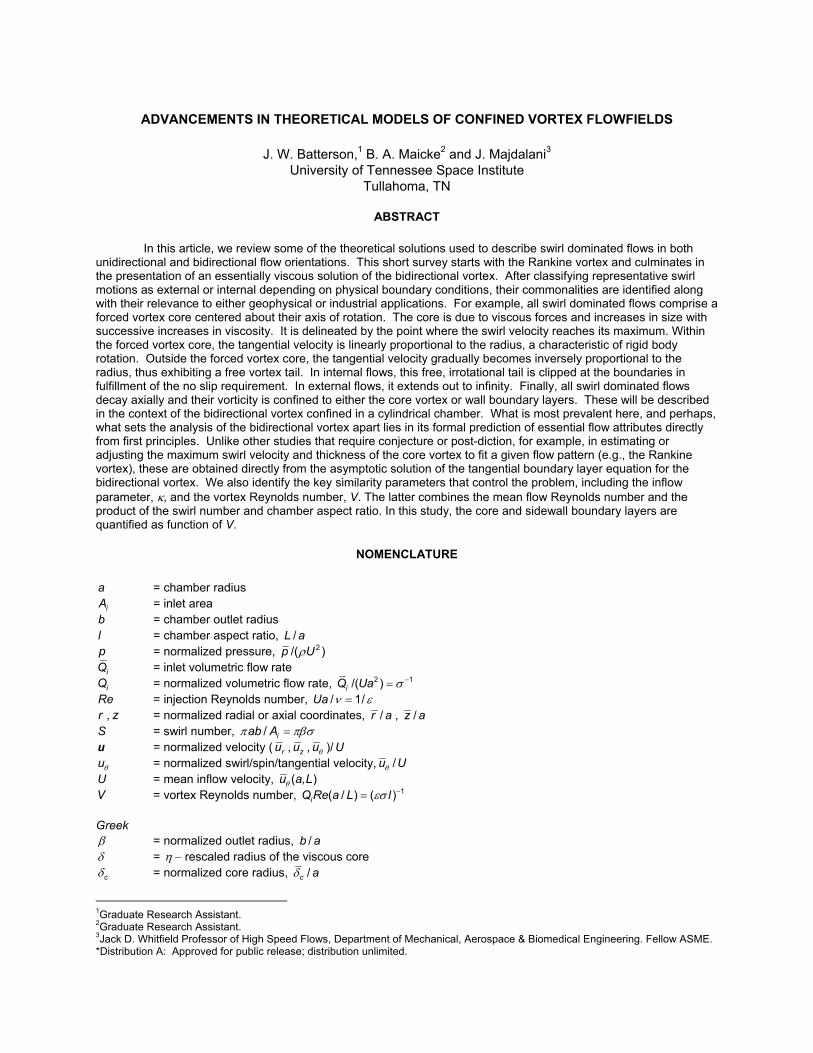
ADVANCEMENTS IN THEORETICAL MODELS OF CONFINED VORTEX FLOWFIELDS

J. W. Batterson,1 B. A. Maicke2 and J. Majdalani3 University of Tennessee Space Institute

Tullahoma, TN

ABSTRACT

In this article, we review some of the theoretical solutions used to describe swirl dominated flows in both unidirectional and bidirectional flow orientations. This short survey starts with the Rankine vortex and culminates in the presentation of an essentially viscous solution of the bidirectional vortex. After classifying representative swirl motions as external or internal depending on physical boundary conditions, their commonalities are identified along with their relevance to either geophysical or industrial applications. For example, all swirl dominated flows comprise a forced vortex core centered about their axis of rotation. The core is due to viscous forces and increases in size with successive increases in viscosity. It is delineated by the point where the swirl velocity reaches its maximum. Within the forced vortex core, the tangential velocity is linearly proportional to the radius, a characteristic of rigid body rotation. Outside the forced vortex core, the tangential velocity gradually becomes inversely proportional to the radius, thus exhibiting a free vortex tail. In internal flows, this free, irrotational tail is clipped at the boundaries in fulfillment of the no slip requirement. In external flows, it extends out to infinity. Finally, all swirl dominated flows decay axially and their vorticity is confined to either the core vortex or wall boundary layers. These will be described in the context of the bidirectional vortex confined in a cylindrical chamber. What is most prevalent here, and perhaps, what sets the analysis of the bidirectional vortex apart lies in its formal prediction of essential flow attributes directly from first principles. Unlike other studies that require conjecture or post-diction, for example, in estimating or adjusting the maximum swirl velocity and thickness of the core vortex to fit a given flow pattern (e.g., the Rankine vortex), these are obtained directly from the asymptotic solution of the tangential boundary layer equation for the bidirectional vortex. We also identify the key similarity parameters that control the problem, including the inflow parameter, κ, and the vortex Reynolds number, V. The latter combines the mean flow Reynolds number and the product of the swirl number and chamber aspect ratio. In this study, the core and sidewall boundary layers are quantified as function of V.

NOMENCLATURE

a = chamber radius iA = inlet area

b = chamber outlet radius l = chamber aspect ratio, /L a p = normalized pressure, ρ 2/( )p U

iQ = inlet volumetric flow rate iQ = normalized volumetric flow rate, σ −=2 1/( )iQ Ua

Re = injection Reynolds number, ν ε=/ 1/Ua r , z = normalized radial or axial coordinates, /r a , /z a S = swirl number, π πβσ=/ iab A u = normalized velocity ( ru , zu , θu )/U θu = normalized swirl/spin/tangential velocity, θ /u U

U = mean inflow velocity, θ ( , )u a L V = vortex Reynolds number, εσ −= 1( / ) ( )iQ Re a L l Greek β = normalized outlet radius, /b a δ = η − rescaled radius of the viscous core δc = normalized core radius, δ /c a

1Graduate Research Assistant. 2Graduate Research Assistant. 3Jack D. Whitfield Professor of High Speed Flows, Department of Mechanical, Aerospace & Biomedical Engineering. Fellow ASME. *Distribution A: Approved for public release; distribution unlimited.

δw = wall tangential boundary layer thickness, δ /w a ε = perturbation parameter, ν=1/ /( )Re Ua κ = inflow parameter, π πσ −= 1/(2 ) (2 )iQ l l λ = η − rescaled wall layer thickness, λ / a ν = kinematic viscosity, μ ρ/ η = transformed variable, π 2r ρ = density σ = modified swirl number, πβ− =1 /( )iQ S Subscripts i = inlet property r = radial component or partial derivative z = axial component or partial derivative θ = azimuthal component or partial derivative

= overbars denote dimensional variables Superscripts c = composite i = inner core w = near sidewall

INTRODUCTION

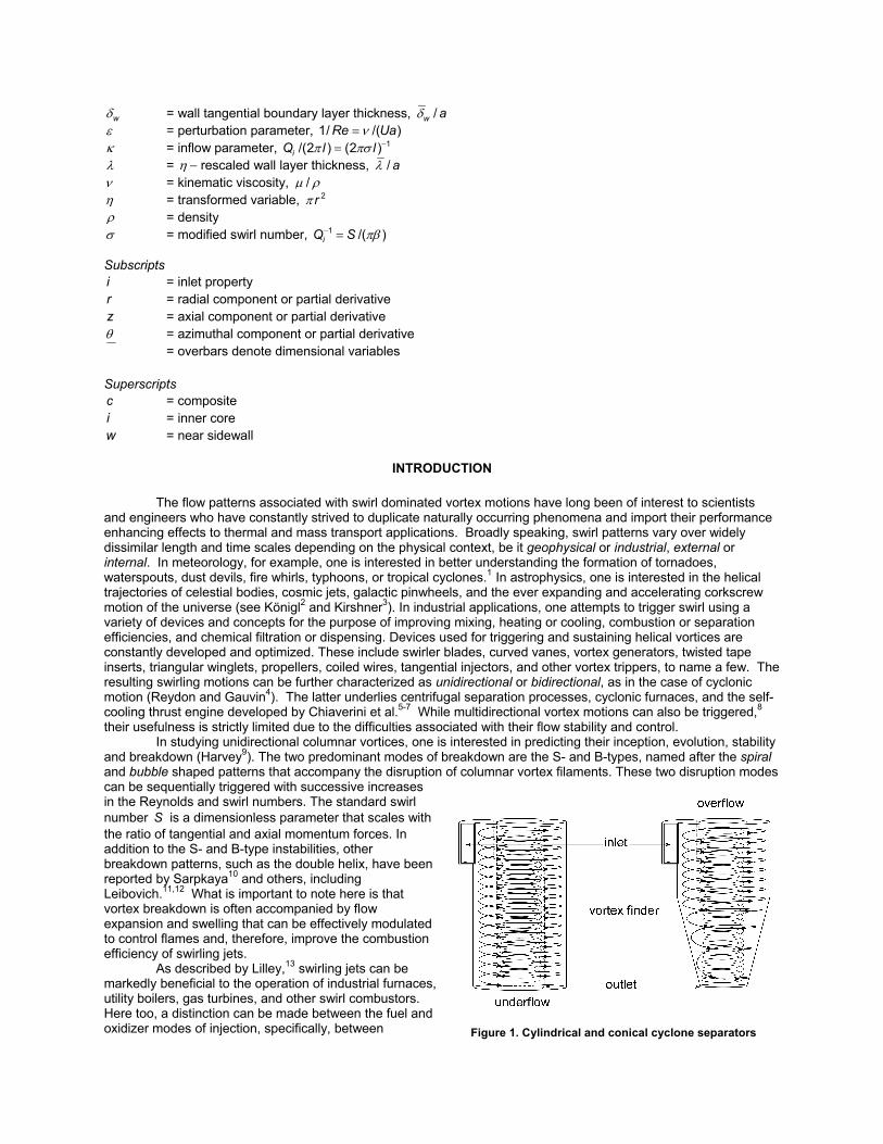
The flow patterns associated with swirl dominated vortex motions have long been of interest to scientists and engineers who have constantly strived to duplicate naturally occurring phenomena and import their performance enhancing effects to thermal and mass transport applications. Broadly speaking, swirl patterns vary over widely dissimilar length and time scales depending on the physical context, be it geophysical or industrial, external or internal. In meteorology, for example, one is interested in better understanding the formation of tornadoes, waterspouts, dust devils, fire whirls, typhoons, or tropical cyclones.1 In astrophysics, one is interested in the helical trajectories of celestial bodies, cosmic jets, galactic pinwheels, and the ever expanding and accelerating corkscrew motion of the universe (see Königl2 and Kirshner3). In industrial applications, one attempts to trigger swirl using a variety of devices and concepts for the purpose of improving mixing, heating or cooling, combustion or separation efficiencies, and chemical filtration or dispensing. Devices used for triggering and sustaining helical vortices are constantly developed and optimized. These include swirler blades, curved vanes, vortex generators, twisted tape inserts, triangular winglets, propellers, coiled wires, tangential injectors, and other vortex trippers, to name a few. The resulting swirling motions can be further characterized as unidirectional or bidirectional, as in the case of cyclonic motion (Reydon and Gauvin4). The latter underlies centrifugal separation processes, cyclonic furnaces, and the self-cooling thrust engine developed by Chiaverini et al.5-7 While multidirectional vortex motions can also be triggered,8 their usefulness is strictly limited due to the difficulties associated with their flow stability and control. In studying unidirectional columnar vortices, one is interested in predicting their inception, evolution, stability and breakdown (Harvey9). The two predominant modes of breakdown are the S- and B-types, named after the spiral and bubble shaped patterns that accompany the disruption of columnar vortex filaments. These two disruption modes can be sequentially triggered with successive increases in the Reynolds and swirl numbers. The standard swirl number S is a dimensionless parameter that scales with the ratio of tangential and axial momentum forces. In addition to the S- and B-type instabilities, other breakdown patterns, such as the double helix, have been reported by Sarpkaya10 and others, including Leibovich.11,12 What is important to note here is that vortex breakdown is often accompanied by flow expansion and swelling that can be effectively modulated to control flames and, therefore, improve the combustion efficiency of swirling jets. As described by Lilley,13 swirling jets can be markedly beneficial to the operation of industrial furnaces, utility boilers, gas turbines, and other swirl combustors. Here too, a distinction can be made between the fuel and oxidizer modes of injection, specifically, between

Figure 1. Cylindrical and conical cyclone separators

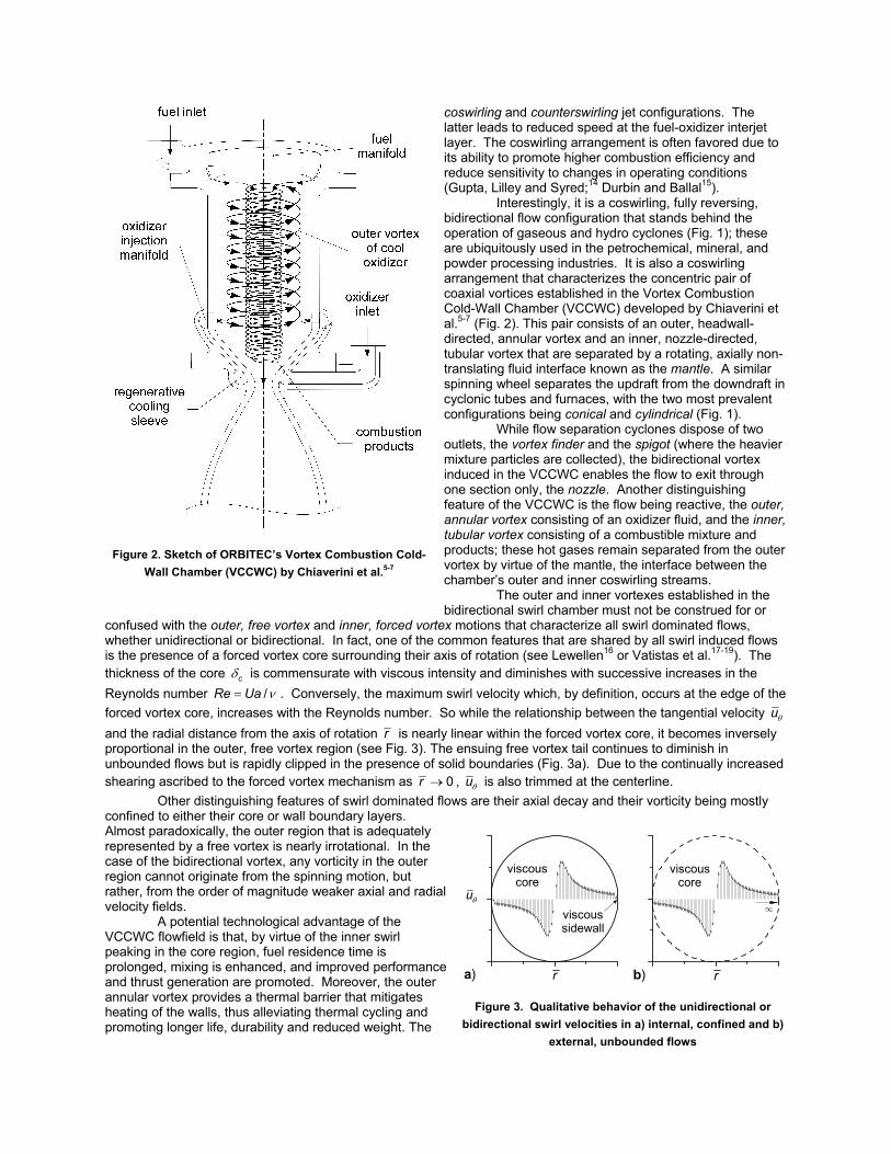
coswirling and counterswirling jet configurations. The latter leads to reduced speed at the fuel-oxidizer interjet layer. The coswirling arrangement is often favored due to its ability to promote higher combustion efficiency and reduce sensitivity to changes in operating conditions (Gupta, Lilley and Syred;14 Durbin and Ballal15). Interestingly, it is a coswirling, fully reversing, bidirectional flow configuration that stands behind the operation of gaseous and hydro cyclones (Fig. 1); these are ubiquitously used in the petrochemical, mineral, and powder processing industries. It is also a coswirling arrangement that characterizes the concentric pair of coaxial vortices established in the Vortex Combustion Cold-Wall Chamber (VCCWC) developed by Chiaverini et al.5-7 (Fig. 2). This pair consists of an outer, headwall-directed, annular vortex and an inner, nozzle-directed, tubular vortex that are separated by a rotating, axially non-translating fluid interface known as the mantle. A similar spinning wheel separates the updraft from the downdraft in cyclonic tubes and furnaces, with the two most prevalent configurations being conical and cylindrical (Fig. 1). While flow separation cyclones dispose of two outlets, the vortex finder and the spigot (where the heavier mixture particles are collected), the bidirectional vortex induced in the VCCWC enables the flow to exit through one section only, the nozzle. Another distinguishing feature of the VCCWC is the flow being reactive, the outer, annular vortex consisting of an oxidizer fluid, and the inner, tubular vortex consisting of a combustible mixture and products; these hot gases remain separated from the outer vortex by virtue of the mantle, the interface between the chamber’s outer and inner coswirling streams. The outer and inner vortexes established in the bidirectional swirl chamber must not be construed for or

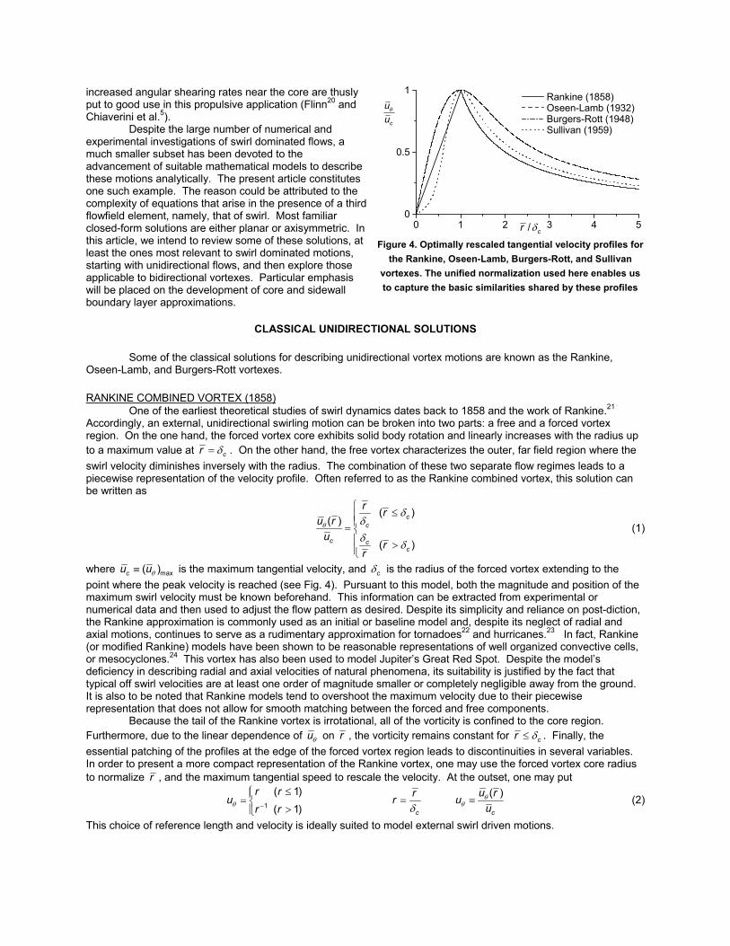
confused with the outer, free vortex and inner, forced vortex motions that characterize all swirl dominated flows, whether unidirectional or bidirectional. In fact, one of the common features that are shared by all swirl induced flows is the presence of a forced vortex core surrounding their axis of rotation (see Lewellen16 or Vatistas et al.17-19). The thickness of the core δc is commensurate with viscous intensity and diminishes with successive increases in the Reynolds number ν= /Re Ua . Conversely, the maximum swirl velocity which, by definition, occurs at the edge of the forced vortex core, increases with the Reynolds number. So while the relationship between the tangential velocity θu and the radial distance from the axis of rotation r is nearly linear within the forced vortex core, it becomes inversely proportional in the outer, free vortex region (see Fig. 3). The ensuing free vortex tail continues to diminish in unbounded flows but is rapidly clipped in the presence of solid boundaries (Fig. 3a). Due to the continually increased shearing ascribed to the forced vortex mechanism as → 0r , θu is also trimmed at the centerline. Other distinguishing features of swirl dominated flows are their axial decay and their vorticity being mostly confined to either their core or wall boundary layers. Almost paradoxically, the outer region that is adequately represented by a free vortex is nearly irrotational. In the case of the bidirectional vortex, any vorticity in the outer region cannot originate from the spinning motion, but rather, from the order of magnitude weaker axial and radial velocity fields. A potential technological advantage of the VCCWC flowfield is that, by virtue of the inner swirl peaking in the core region, fuel residence time is prolonged, mixing is enhanced, and improved performance and thrust generation are promoted. Moreover, the outer annular vortex provides a thermal barrier that mitigates heating of the walls, thus alleviating thermal cycling and promoting longer life, durability and reduced weight. The

r

θuviscoussidewall

viscouscore

a) rb)

∞

viscouscore

Figure 3. Qualitative behavior of the unidirectional or bidirectional swirl velocities in a) internal, confined and b)

external, unbounded flows

Figure 2. Sketch of ORBITEC’s Vortex Combustion Cold-Wall Chamber (VCCWC) by Chiaverini et al.5-7

increased angular shearing rates near the core are thusly put to good use in this propulsive application (Flinn20 and Chiaverini et al.5). Despite the large number of numerical and experimental investigations of swirl dominated flows, a much smaller subset has been devoted to the advancement of suitable mathematical models to describe these motions analytically. The present article constitutes one such example. The reason could be attributed to the complexity of equations that arise in the presence of a third flowfield element, namely, that of swirl. Most familiar closed-form solutions are either planar or axisymmetric. In this article, we intend to review some of these solutions, at least the ones most relevant to swirl dominated motions, starting with unidirectional flows, and then explore those applicable to bidirectional vortexes. Particular emphasis will be placed on the development of core and sidewall boundary layer approximations.

CLASSICAL UNIDIRECTIONAL SOLUTIONS

Some of the classical solutions for describing unidirectional vortex motions are known as the Rankine, Oseen-Lamb, and Burgers-Rott vortexes.

RANKINE COMBINED VORTEX (1858) One of the earliest theoretical studies of swirl dynamics dates back to 1858 and the work of Rankine.21 Accordingly, an external, unidirectional swirling motion can be broken into two parts: a free and a forced vortex region. On the one hand, the forced vortex core exhibits solid body rotation and linearly increases with the radius up to a maximum value at δ= cr . On the other hand, the free vortex characterizes the outer, far field region where the swirl velocity diminishes inversely with the radius. The combination of these two separate flow regimes leads to a piecewise representation of the velocity profile. Often referred to as the Rankine combined vortex, this solution can be written as

θ

δδδ

δ

⎧ ≤⎪⎪= ⎨⎪ >⎪⎩

( )( )

( )

cc

c cc

r ru r

ur

r

(1)

where θ≡ max( )cu u is the maximum tangential velocity, and δc is the radius of the forced vortex extending to the point where the peak velocity is reached (see Fig. 4). Pursuant to this model, both the magnitude and position of the maximum swirl velocity must be known beforehand. This information can be extracted from experimental or numerical data and then used to adjust the flow pattern as desired. Despite its simplicity and reliance on post-diction, the Rankine approximation is commonly used as an initial or baseline model and, despite its neglect of radial and axial motions, continues to serve as a rudimentary approximation for tornadoes22 and hurricanes.23 In fact, Rankine (or modified Rankine) models have been shown to be reasonable representations of well organized convective cells, or mesocyclones.24 This vortex has also been used to model Jupiter’s Great Red Spot. Despite the model’s deficiency in describing radial and axial velocities of natural phenomena, its suitability is justified by the fact that typical off swirl velocities are at least one order of magnitude smaller or completely negligible away from the ground. It is also to be noted that Rankine models tend to overshoot the maximum velocity due to their piecewise representation that does not allow for smooth matching between the forced and free components. Because the tail of the Rankine vortex is irrotational, all of the vorticity is confined to the core region. Furthermore, due to the linear dependence of θu on r , the vorticity remains constant for δ≤ cr . Finally, the essential patching of the profiles at the edge of the forced vortex region leads to discontinuities in several variables. In order to present a more compact representation of the Rankine vortex, one may use the forced vortex core radius to normalize r , and the maximum tangential speed to rescale the velocity. At the outset, one may put

θ −

≤⎧⎪= ⎨>⎪⎩

1

( 1)( 1)

r ru

r r

δ=

c

rr θθ ≡

( )

c

u ruu

(2)

This choice of reference length and velocity is ideally suited to model external swirl driven motions.

0 1 2 3 4 50

0.5

1

δ/ cr

θ

c

uu

Rankine (1858) Oseen-Lamb (1932) Burgers-Rott (1948) Sullivan (1959)

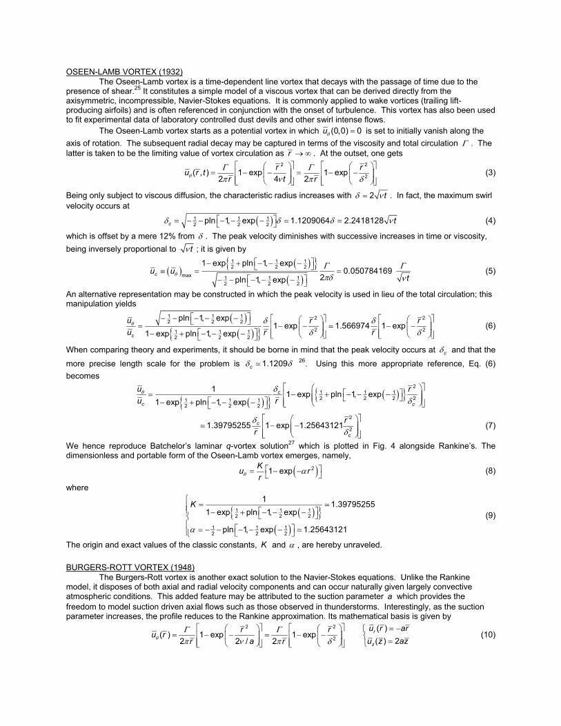
Figure 4. Optimally rescaled tangential velocity profiles for

the Rankine, Oseen-Lamb, Burgers-Rott, and Sullivan vortexes. The unified normalization used here enables us to capture the basic similarities shared by these profiles

OSEEN-LAMB VORTEX (1932) The Oseen-Lamb vortex is a time-dependent line vortex that decays with the passage of time due to the presence of shear.25 It constitutes a simple model of a viscous vortex that can be derived directly from the axisymmetric, incompressible, Navier-Stokes equations. It is commonly applied to wake vortices (trailing lift-producing airfoils) and is often referenced in conjunction with the onset of turbulence. This vortex has also been used to fit experimental data of laboratory controlled dust devils and other swirl intense flows. The Oseen-Lamb vortex starts as a potential vortex in which θ =(0,0) 0u is set to initially vanish along the axis of rotation. The subsequent radial decay may be captured in terms of the viscosity and total circulation Γ . The latter is taken to be the limiting value of vortex circulation as →∞r . At the outset, one gets

θΓ Γπ ν π δ

⎡ ⎤⎡ ⎤ ⎛ ⎞⎛ ⎞= − − = − −⎢ ⎥⎢ ⎥ ⎜ ⎟⎜ ⎟

⎢ ⎥ ⎢ ⎥⎝ ⎠ ⎝ ⎠⎣ ⎦ ⎣ ⎦

2 2

2( , ) 1 exp 1 exp2 4 2

r ru r tr t r

(3)

Being only subject to viscous diffusion, the characteristic radius increases with δ ν= 2 t . In fact, the maximum swirl velocity occurs at

( )δ δ δ ν⎡ ⎤= − − − − − =⎣ ⎦1 1 12 2 2pln 1, exp 1.1209064 2.2418128c t (4)

which is offset by a mere 12% from δ . The peak velocity diminishes with successive increases in time or viscosity, being inversely proportional to ν t ; it is given by

( )( )

( )θ

Γ Γπδ ν

⎡ ⎤− + − − −⎣ ⎦≡ = =⎡ ⎤− − − − −⎣ ⎦

1 1 12 2 2

max 1 1 12 2 2

1 exp pln 1, exp0.050784169

2pln 1, expcu u

t (5)

An alternative representation may be constructed in which the peak velocity is used in lieu of the total circulation; this manipulation yields

( )( )

θ δ δδ δ

⎡ ⎤− − − − − ⎡ ⎤ ⎡ ⎤⎛ ⎞ ⎛ ⎞⎣ ⎦= − − − −⎢ ⎥ ⎢ ⎥⎜ ⎟ ⎜ ⎟⎡ ⎤− + − − − ⎢ ⎥ ⎢ ⎥⎝ ⎠ ⎝ ⎠⎣ ⎦ ⎣ ⎦⎣ ⎦

1 1 1 2 22 2 2

2 21 1 12 2 2

pln 1, exp1 exp 1.566974 1 exp

1 exp pln 1, expc

u r ru r r

(6)

When comparing theory and experiments, it should be borne in mind that the peak velocity occurs at δc and that the

more precise length scale for the problem is δ δ1.1209c 26. Using this more appropriate reference, Eq. (6) becomes

( ) ( ) θ δ

δ

⎡ ⎤⎛ ⎞⎡ ⎤= − + − − −⎢ ⎥⎜ ⎟⎣ ⎦⎜ ⎟⎡ ⎤− + − − − ⎢ ⎥⎝ ⎠⎣ ⎦⎣ ⎦

21 1 12 2 2 21 1 1

2 2 2

1 1 exp pln 1, exp1 exp pln 1, exp

c

c c

u ru r

δδ

⎡ ⎤⎛ ⎞− −⎢ ⎥⎜ ⎟⎜ ⎟⎢ ⎥⎝ ⎠⎣ ⎦

2

21.39795255 1 exp 1.25643121c

c

rr

(7)

We hence reproduce Batchelor’s laminar q-vortex solution27 which is plotted in Fig. 4 alongside Rankine’s. The dimensionless and portable form of the Oseen-Lamb vortex emerges, namely,

( )θ α⎡ ⎤= − −⎣ ⎦21 expKu r

r (8)

where

( ) ( )α

⎧ =⎪⎪ ⎡ ⎤− + − − −⎣ ⎦⎨⎪ ⎡ ⎤= − − − − −⎪ ⎣ ⎦⎩

1 1 12 2 2

1 1 12 2 2

1 1.397952551 exp pln 1, exp

pln 1, exp 1.25643121

K

(9)

The origin and exact values of the classic constants, K and α , are hereby unraveled.

BURGERS-ROTT VORTEX (1948) The Burgers-Rott vortex is another exact solution to the Navier-Stokes equations. Unlike the Rankine model, it disposes of both axial and radial velocity components and can occur naturally given largely convective atmospheric conditions. This added feature may be attributed to the suction parameter a which provides the freedom to model suction driven axial flows such as those observed in thunderstorms. Interestingly, as the suction parameter increases, the profile reduces to the Rankine approximation. Its mathematical basis is given by

θΓ Γπ ν π δ

⎡ ⎤⎡ ⎤ = −⎛ ⎞⎛ ⎞ ⎧= − − = − −⎢ ⎥⎢ ⎥ ⎜ ⎟⎜ ⎟ ⎨

=⎢ ⎥ ⎢ ⎥ ⎩⎝ ⎠ ⎝ ⎠⎣ ⎦ ⎣ ⎦

2 2

2

( )( ) 1 exp 1 exp

( ) 22 2 / 2r

z

u r arr ru ru z azr a r

(10)

where δ ν= 2 / a . Clearly, when the radius is normalized by δ , this profile becomes identical to the Oseen-Lamb expression. Both are superimposed in Fig. 4. Based on Eq. (5), the peak swirl can be calculated to be

( )

( )Γ Γ Γπδ πδ ν

⎡ ⎤− + − − −⎣ ⎦= =⎡ ⎤− − − − −⎣ ⎦

1 1 12 2 2

1 1 12 2 2

1 exp pln 1, exp0.638172686 0.07181966

2 2 /pln 1, expcu

a (11)

It should also be noted that both the Burgers-Rott and Oseen-Lamb vortexes are axisymmetric Gaussian solutions of the incompressible Navier-Stokes equations. Both can be expressed as

( )θ Γδ π

−⎛ ⎞= =⎜ ⎟⎝ ⎠

214

1;4

xru G G x e (12)

where ( )G x is the normalized Gaussian function, and ( Γ , δ ) denote their circulation and core characteristic scale. Despite their simplicity, these solutions continue to receive attention. Examples abound and one may cite those by Schmid and Rossi,28 Pérez-Saborid et al.,29 Eloy and Le Dizès,30 Alekseenko et al.,26 and Devenport et al.31 In several experiments, empirical relations are developed based on Eq. (10), specifically,

θ π δ δ⎡ ⎤⎛ ⎞ ⎛ ⎞

= − − = + −⎢ ⎥⎜ ⎟ ⎜ ⎟⎢ ⎥⎝ ⎠ ⎝ ⎠⎣ ⎦

2 2

1 22 21 exp ; exp2 zK r ru u W W

r (13)

where δ 1, , ,K W and 2W are constants that are determined empirically (see Leibovich,11,12 Faler and Leibovich,32 and Escudier33). Several other solutions are derived in similar context and described by Long,34 Alekseenko et al.,26 and others. The Oseen-Lamb and Burgers-Rott vortexes are closely related as both can be described by the Gaussian function. They differ primarily in the fact that the Oseen-Lamb vortex displays temporal diffusion. At first glance one might expect the Burgers-Rott vortex to be more useful in predicting naturally occurring vortices due to the appearance of axial and radial velocity components and the parallelism between the suction parameter and the convective nature of large thunderstorms. Indeed at large suction values the Burgers-Rott vortex approaches the classical Rankine model. With caution this vortex can be applied to atmospheric swirl patterns. However, the characteristic that the axial velocity increases without bound suggests that the suction source is located at infinity. This vortex can hence be applied to near ground scenarios. The height of validity from the ground is subject to the areal expanse of the storm compared to the localized vortex as well as the altitude at which the convective rise dissipates. Consequently, large rotating thunderheads should be omitted from the application of this model and rather the scope should be narrowed to localized swirls such as tornados.

CLASSICAL BIDIRECTIONAL SOLUTIONS

Solutions that represent bidirectional vortex motions are much less common in the literature. Here we consider those by Sullivan,35 Bloor and Ingham,36 and Vyas and Majdalani.37

SULLIVAN’S VORTEX (1959) Sullivan’s vortex is an exact viscous solution to the Navier-Stokes equations in an unbounded domain.35 This profile corresponds to a two-cell structure; its inner cell comprises a region where fluid is in constant descent and then flows outwardly to rejoin a separate flow converging radially. It thus captures physical mechanisms exhibiting a distinct inner downflow. Because of this two-cell behavior, the Sullivan vortex is used in meteorological studies to simulate the flow generated by tornados;38 these display an intense downdraft at the core surrounded by localized updrafts. The Sullivan model can also be used as a starting point for the modeling of hurricanes.39 However, its prediction of a significant swirl velocity near the core is not observed in hurricanes, so current studies often extend and modify the Sullivan vortex to address the discrepancies between theoretical results and observed behavior. Mathematically, its integral representation consists of

( ) ( )

( )

θΓ Γπ υ π δ

−

⎧ ⎛ ⎞⎛ ⎞= =⎪ ⎜ ⎟⎜ ⎟

∞ ∞⎪ ⎝ ⎠ ⎝ ⎠⎨⎪ = = − + −⎪⎩

∫ ∫

2 2

2

( )0 0

1 1( )2 2 / 2

d( ) d ; ( ) 3 1x tf t y

r ru r H Hr H a r H

yH x e t f t t ey

(14)

Note that the radial and axial velocity companions are given by

υδ δ

⎡ ⎤ ⎡ ⎤⎛ ⎞ ⎛ ⎞= − + − − = − −⎢ ⎥ ⎢ ⎥⎜ ⎟ ⎜ ⎟

⎢ ⎥ ⎢ ⎥⎝ ⎠ ⎝ ⎠⎣ ⎦ ⎣ ⎦

2 2

2 26( ) 1 exp ( , ) 2 1 3expr z

r ru r ar u r z azr

(15)

where δ υ= 2 / a ; a is the suction strength and υ is the viscosity dominated by the eddy viscosity. At first glance, the integral ( )f t in Eq. (14) may appear to diverge. However, as the function is integrated, its contribution becomes

negligible past a radial position corresponding to = 10x . For this reason, we see a strong resemblance in the tail region to that of a Rankine vortex. The peak circumferential velocity will occur when θ′ =( ) 0u r or

( ) ( ) ( ) δϒ δδ ϒ δ δ

− +⎡ ⎤− − + + + = =⎣ ⎦∫

EE

2 22 2 2 /3 3 0, /8

02 / exp 3 0, ln( ) d 0; 2.49761606

rr rcr e t t t t (16)

where E 0.57721566 is Euler’s gamma constant and ϒ is Euler’s gamma function. A rescaled representation of Sullivan’s vortex can be achieved using

( )

δΓ Γ Γπδ δδ υ

⎛ ⎞= ⎜ ⎟⎜ ⎟∞ ⎝ ⎠

2

21 0.0567688 =0.0401416

2 /c

cc

u HH a

(17)

and so,

( ) ( )θΓ Γπ υ π δ

⎛ ⎞⎛ ⎞= = ⎜ ⎟⎜ ⎟ ⎜ ⎟∞ ∞⎝ ⎠ ⎝ ⎠

2 2

21 2.497616 6.23809

2 2 / 2 c

r ru H Hr H a r H

(18)

Subsequent normalization by the maximum velocity yields

( ) ( )θ

θδ

δ⎛ ⎞

= = ⎜ ⎟⎜ ⎟⎝ ⎠

22

21 0.02989026.23809 6.23809

6.23809c

c c

u ru H H ru H r r

(19)

One may note the similarities among the foregoing solutions in Fig. 4.

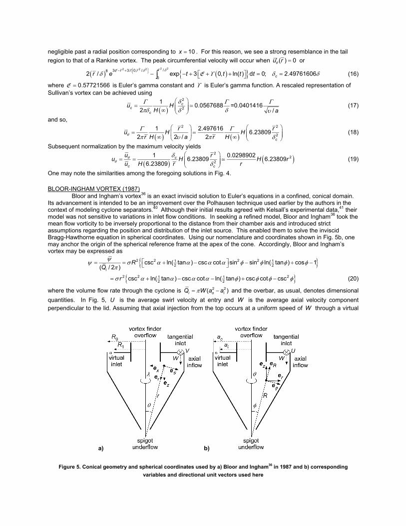
BLOOR-INGHAM VORTEX (1987) Bloor and Ingham’s vortex36 is an exact inviscid solution to Euler’s equations in a confined, conical domain. Its advancement is intended to be an improvement over the Polhausen technique used earlier by the authors in the context of modeling cyclone separators.40 Although their initial results agreed with Kelsall’s experimental data,41 their model was not sensitive to variations in inlet flow conditions. In seeking a refined model, Bloor and Ingham36 took the mean flow vorticity to be inversely proportional to the distance from their chamber axis and introduced strict assumptions regarding the position and distribution of the inlet source. This enabled them to solve the inviscid Bragg-Hawthorne equation in spherical coordinates. Using our nomenclature and coordinates shown in Fig. 5b, one may anchor the origin of the spherical reference frame at the apex of the cone. Accordingly, Bloor and Ingham’s vortex may be expressed as

ψψ σ α α α α φ φ φ φπ

⎡ ⎤= = + − − + −⎣ ⎦2 2 2 21 1

2 2csc ln( tan ) csc cot sin sin ln( tan ) cos 1( / 2 )i

RQ

σ α α α α φ φ φ φ= + − − + −2 2 21 12 2csc ln( tan ) csc cot ln( tan ) csc cot cscr (20)

where the volume flow rate through the cyclone is π= −2 2( )i o iQ W a a and the overbar, as usual, denotes dimensional quantities. In Fig. 5, U is the average swirl velocity at entry and W is the average axial velocity component perpendicular to the lid. Assuming that axial injection from the top occurs at a uniform speed of W through a virtual

a) b)

Figure 5. Conical geometry and spherical coordinates used by a) Bloor and Ingham36 in 1987 and b) corresponding variables and directional unit vectors used here

opening, < <i oa r a , neither W nor ia are known at the outset because “they depend on the way in which the three-dimensional flow in the cylindrical section of the cyclone develops into the axially symmetric flow.” Unlike external flows in which the radial distance to the peak swirl velocity is taken to be the characteristic length, it is convenient to normalize radial and axial coordinates by ≡oa a ; the dimensionless parameter σ is given by

π

σ = =−

2 2 2 2

2 2/

(1 / )o

i oi

a U U Wa aQW

(21)

This can be obtained from Eq. (25) in Bloor and Ingham.36 The spherical solution comprises

( )σ α α α α φ σ φ φπ

⎡ ⎤⎡ ⎤= = + − −⎣ ⎦ ⎣ ⎦2 1 1

2 22 2 csc ln( tan ) csc cot cos 2 cos ln tan( / 2 )

RR

i

uuQ a

(22)

φφ

ψφπ

= =22

sin2( / 2 )i

uu

Q a θ

θσψ

π= = −

2

2 2 21 1 iu Qu

U r a U (23)

It is valid for < <0 1r and becomes singular along the axis of the cyclone. When reverting back to cylindrical coordinates, one may use φ φφ φ φ φ= − = +sin cos cos sinr R z Ru u u u u u (24) Note that the tangential velocity is normalized differently from the rest, being referenced to the average tangential velocity at entry. For small divergence angles of the conical chamber, one recovers ( ) ( )2 2 2ln / csc 2( 1)ln / 1zr uψ σ φ φ α φ σ φ φ α⎡ ⎤= − = − + +⎣ ⎦ (25)

VYAS-MAJDALANI VORTEX (2003)

The Vyas-Majdalani vortex is an exact inviscid solution to Euler’s equations derived in a confined, cylindrical domain. It is obtained using the vorticity-stream function approach and a novel technique introduced by Vyas, Majdalani and Chiaverini,42 and later refined by Vyas and Majdalani.37 This technique is extended to spherical geometry by Majdalani and Rienstra43 wherein the existence of additional exact solutions is demonstrated. The Vyas-Majdalani vortex shares similar features to those associated with Bloor and Ingham’s, including the inviscid singularity at the origin. However, it is not limited to the assumptions made previously, such as the requirement on the vorticity to remain inversely proportional to the radial distance throughout the chamber. The singularity at the origin is a known characteristic of inviscidly swirling motions and adds some reassurance to the results of Vyas and Majdalani;37 the singularity can actually be overcome by regularizing the tangential momentum equation before applying matched-asymptotic expansions.44 Another interesting outcome of the inviscid model stems from its ability to predict the existence of multiple mantles in a cylindrical cyclone, as shown in a companion paper by Vyas, Majdalani and Chiaverini.8 What was considered to be unlikely at first was confirmed, that same year, through the extensive laboratory and numerical experiments carried out independently by Anderson et al.45 In order to capture the sidewall boundary layers, Vyas and Majdalani have rescaled the tangential momentum equation and constructed a composite solution for the swirl velocity. This is an essential first step for a variety of reasons. Their approximation for the swirl velocity remains uniformly valid from the core to the sidewall, inclusively.46 Along similar lines, Batterson and Majdalani47 have rescaled the axial and radial momentum equations and provided an improved rotational, incompressible, steady-state solution for the problem at hand. The no slip condition is thus observed in all three directions. Parallel efforts have been carried out by Maicke and Majdalani48 for the purpose of producing a fully compressible approximation. Theirs is based on a Rayleigh-Janzen expansion that has proved successful in the treatment of compressible Taylor and Culick profiles.49-51 Such profiles are parameter-free, inviscid, rotational, and non-swirling; nonetheless, they are ubiquitously used and shown to be adequate models for the internal flowfield in solid rocket motors. In what follows, some of these developments are briefly described.

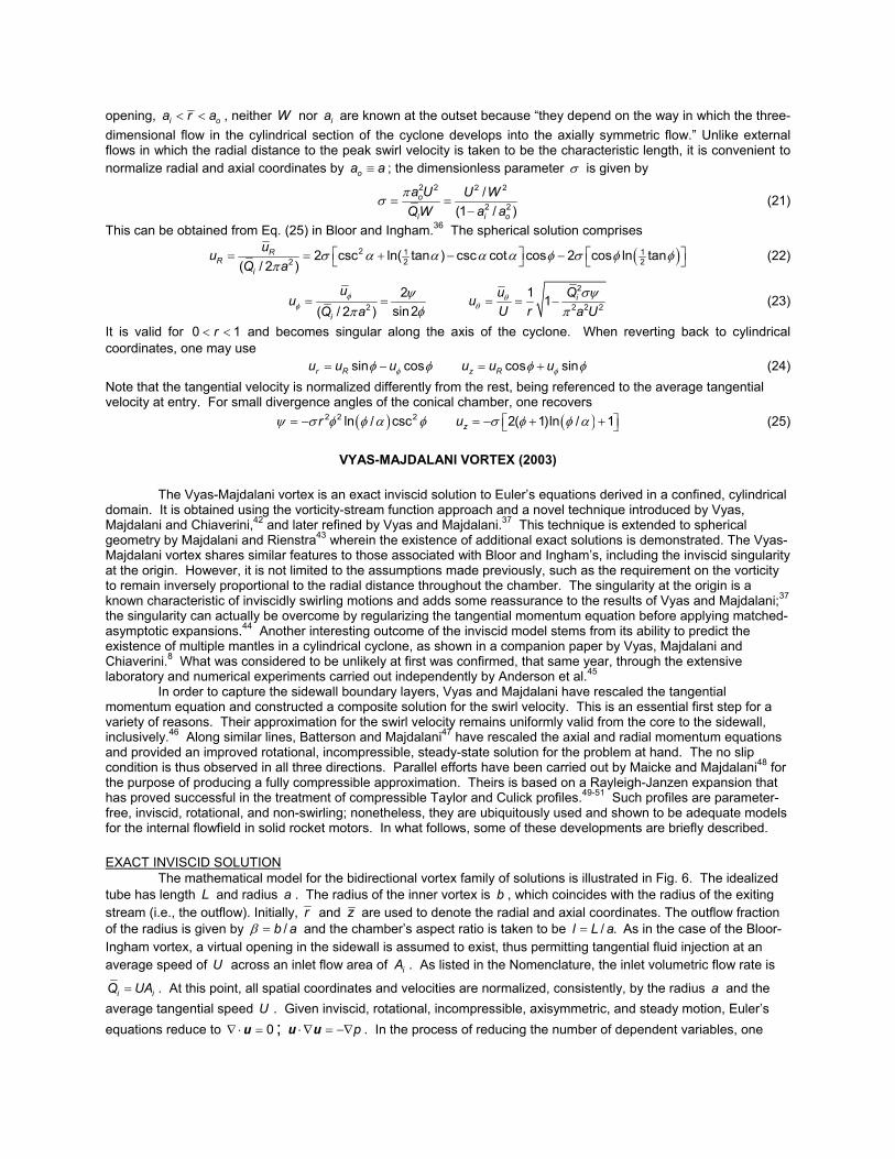
EXACT INVISCID SOLUTION The mathematical model for the bidirectional vortex family of solutions is illustrated in Fig. 6. The idealized tube has length L and radius a . The radius of the inner vortex is b , which coincides with the radius of the exiting stream (i.e., the outflow). Initially, r and z are used to denote the radial and axial coordinates. The outflow fraction of the radius is given by β = /b a and the chamber’s aspect ratio is taken to be = / .l L a As in the case of the Bloor-Ingham vortex, a virtual opening in the sidewall is assumed to exist, thus permitting tangential fluid injection at an average speed of U across an inlet flow area of iA . As listed in the Nomenclature, the inlet volumetric flow rate is

=i iQ UA . At this point, all spatial coordinates and velocities are normalized, consistently, by the radius a and the average tangential speed U . Given inviscid, rotational, incompressible, axisymmetric, and steady motion, Euler’s equations reduce to ∇ ⋅ = 0u ; ⋅∇ = −∇pu u . In the process of reducing the number of dependent variables, one

eliminates the pressure and introduces the vorticity transport equation, ∇× × =Ω( ) 0u . One also introduces the Stokes stream function through the use of

ψ ψ∂ ∂= − =

∂ ∂1 1; r zu ur z r r

(26)

so continuity is secured. The vorticity stream function will be satisfied, in turn, when a specific connection is found between mean flow vorticity and the stream function, specifically, when θΩ ψ= ( )rF . Following standard practice, we

choose ψ= 2F C and substitute into the vorticity equation. We retrieve the reduced form of the Bragg-Hawthorne equation, namely,

θψ ψ ψΩ ∂ ∂ ∂

= − −∂ ∂ ∂

2 2

2 21rr r r z

or ψ ψ ψ ψ∂ ∂ ∂+ − + =

∂∂ ∂

2 22 2

2 21 0C rr rz r

(27)

At this juncture, separation of variables precipitates ( ) ( ) ( )ψ ⎡ ⎤= + +⎣ ⎦2 21 1

1 2 3 42 2sin cosC z C C Cr C Cr . This can be

readily solved given a judicious assortment of boundary conditions. For the problem at hand, we have (a) tangential injection or θ =(1, ) 1u l ;

(b) no flow penetration at the headwall or =( ,0) 0zu r ;

(c) no asymmetry with respect to the centerline or =(0, ) 0ru z ;

(d) no flow penetration at the sidewall or =(1, ) 0ru z ;

(e) mass balance between inflow and outflow or β

π= =∫02 ( , ) do z iQ u r l r r Q .

Condition (a) can be readily used in conjunction with the conservation principle of angular momentum, given a frictionless fluid, to recover the free vortex θ

−= 1( )u r r . The remaining conditions can be written in terms of the Stokes stream function and rearranged to produce

( )

π β

ψ ψψθψ

= → = → ∂ ∂ =⎧ = → = → ∂ ∂ =⎧⎪⎨ ⎨ = → = → ∂ ∂ == → =∂ ∂ ⎩⎪⎩ ∫ ∫

2

0 0

0 0 / 0 0 0 / 01 0 / 0 d d/

z r

ri

z u r r u zr u zz l r Qr

(28)

where σ −= =2 1/( )i iQ Q Ua is inversely proportional to the modified swirl number σ . The solution to Eq. (27) can be retrieved using the four requirements enumerated in Eq. (28). One recovers π= 2C m and

θκψ κ π π π πκ π

πσ= = = − + +e e e2 2 2 21 1sin( ) sin( ) sin( ) 2 cos( )

2 r zzz m r m r m r z m rl r r

u (29)

where m represents the number of mantles, whereas κ and σ represent the dimensionless inflow and swirl parameters. These are determined from

κ σπ πσ π

= = = =21 2

2 2i

i

A aSaL l A

(30)

Note that σ emerges naturally in our work as a result of proper scaling. In relation to the standard swirl number S used by Gupta, Lilley and Syred,14 one gets σ2.22144S . This direct proportionality is, of course, gratifying. Another useful result is the theoretical determination of the mantle location which, according to Eq. (29), occurs at β= = − =1

, 2( ) / , 1,2,3,...,m nr n m n m (31) where n represents the nth internal mantle for a given reversal mode number m .8 The most prevalent case corresponds to = 1m for which the mantle is predicted to occur at the vortex “rms” radius of β =1,1 2 / 2 0.707 .

Figure 6. Sketch of the bidirectional vortex chamber and corresponding coordinate system before variables are

normalized by the radius a

0

a

a bbr_

z_

L

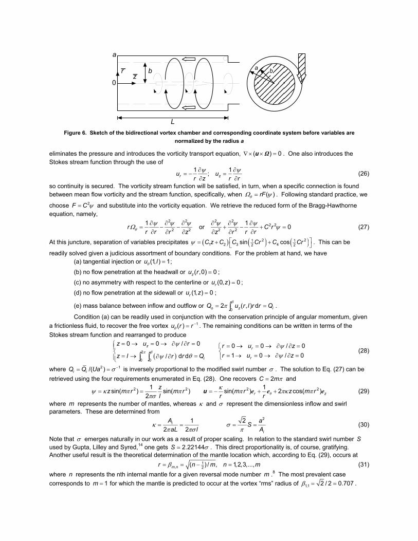
This value is compared in Table 1 to the two cases obtained in a cylindrical cyclone by Smith.52 Note that our idealization is closer to the parameters used in Case II, thus explaining the closer agreement in the last column, with an average of 0.72. The combined average obtained by Smith is 0.67 and may have been influenced by the presence of a vortex finder protruding into the chamber (for the purpose of guiding the outflow). In the case of four mantles, the results so obtained are showcased in Table 2 versus experimental and numerical measurements obtained by Anderson et al.45 It is interesting that Eq. (31) agrees more closely with the experimental results than some numerical simulations. Nonetheless, the set of operating conditions that begets the onset of multiple mantles remains a subject of investigation and conjecture. Before leaving this subject, it should be noted that, in what concerns the swirl number, it is generally defined as the ratio of tangential to axial momentum forces. Its scaling can vary from experiment to experiment, depending on the geometry and scaling used by the authors. For example, Hoekstra, Derksen, and van den Akker53 use

π π πβ= = =

2(2 )(2 )4 4

e

i i

d D b a aSab A A

(32)

where “ ed ” is the diameter of the vortex finder (exit tube), “ ab ” is the tangential inlet area of the cyclone (here, we

use iA instead), and “ D ” is the diameter of the cyclone (here, we use 2a ). It can be easily shown that Eq. (32) reduces to Eq. (30). Conversely, for a combustor with swirl vanes, Lilley13 defines the corresponding swirl number as

φ⎡ ⎤−

= ⎢ ⎥−⎣ ⎦

3

21 ( / )2 tan

3 1 ( / )h

h

d dSd d

(33)

where “ d ” and “ hd ” denote the nozzle diameter and hub diameter of the vanes, and “φ ” stands for the vane angle.

TANGENTIAL BOUNDARY LAYERS The presence of viscosity at the core and sidewall need to be properly accounted for to capture the forced vortex and near-wall decay. The approach we take is to reconsider the tangential momentum equation with viscosity.54 The basic solution of this set is expressible by

θθπκ= − +e e

2sin( ) ( )rr u r

ru zπκ π+ e22 cos( )z r ; κ

π π πσ≡ = =

12 2 2

i iQ Al aL l

(34)

where θ−= 1u r is deficient near = 0r and does not observe the velocity-adherence requirement at the sidewall.

Both problems stem from the absence of viscosity in the leading order, basic model. To overcome these issues, the θ – momentum equation is reconsidered with second-order viscous terms, namely,

( )θθ θ θθ ν

⎡ ⎤∂∂ ∂⎛ ⎞+ = = ≡∇ − ⎢ ⎥⎜ ⎟∂ ∂ ∂⎝ ⎠ ⎣ ⎦2

2

1 1 1 ; rr

ruu u u Uauu Reur r Re Re r r rr

(35)

where Re is the mean flow Reynolds number. Being axially independent, Eq. (35) reduces to

θ θθε ε⎡ ⎤+ = ≡⎢ ⎥⎣ ⎦

d d 1 d 1( ) ; d d d

rr

u u uu rur r r r r Re

(36)

This can be quickly transformed into

ε ξ η ξκ η ηη

+ =2

2d sin d 0

2 dd; θξ ≡ ru ; η π≡ 2r (37)

where κ − −−∼ 3 210 10 . To make further headway, the boundary layers near the core and sidewall must be identified (see Fig. 7). But first, we note that the outer solution may be restored from Eq. (37) by setting ε = 0 . One recovers ξ =( )o C , where (o) denotes an outer approximation and C is a constant.

Table 1 Mantle locations according to Smith52 at MIT

Position Case I

inches

Case II

inches

Case I

normalized

Case II

normalized

1 1.99 2.13 0.6633 0.7083

2 1.89 2.15 0.6300 0.7166

3 1.88 2.15 0.6266 0.7166

4 1.85 2.15 0.6166 0.7166

5 1.79 2.17 0.5966 0.7233

6 1.79 2.20 0.5966 0.7333

7 1.75 2.20 0.5833 0.7333

mean 1.85 2.16 0.6166 0.7211

Table 2 Mantle locations vs. Anderson et al.45 at UW

βexp βanalytic βCFD β β−analytic exp β β−CFD exp

0.296 0.354 0.305 0.058 0.0090.594 0.612 0.385 0.018 0.2090.803 0.791 0.787 0.012 0.0160.955 0.935 1.000 0.020 0.045

INNER, NEAR CORE APPROXIMATION In order to bring the swirl velocity to zero along the chamber axis, one must introduce the slow variable

ηδ ε

≡( )

s (38)

A balance between diffusion and convection near the core leads to the distinguished limit of δ ε κ~ / . The core boundary layer equation becomes exceedingly simple, namely,

ξ ξ+ =

2 ( ) ( )

2d 1 d 0

2 dd

i i

ss;

ξ

ξ ξ

⎧ = = =⎪⎨

→ → ∞ =⎪⎩

( )

( ) ( )

0, 0, 01, ,

i

i o

r sr s

(39)

where the superscript stands for the inner, near-core approximation. Using a series of the form ξ ξ δξ= + +…( ) ( ) ( )0 1

i i i

one retrieves ξ −= −

12( )

0( 1)si C e (40)

Then using Prandtl’s matching principle, we deduce = −0C C . The last constant may be obtained from the downstream condition of a tangentially injected fluid. A composite inner solution is hence determined,

ξ−

−

−=

−

214

14

( ) 11

Vrci

V

ee

or θ

−

−

⎛ ⎞−= ⎜ ⎟⎜ ⎟−⎝ ⎠

214

14

( ) 1 11

Vrci

V

eur e

(41)

where V is the vortex Reynolds number that appears in the problem. This parameter combines the viscous Reynolds number, the swirl number and the geometric aspect ratio:

πκε εσ σ ν

≡ = = =2 1 iQRe aV

l L L (42)

It may be interesting to note the qualitative resemblance between Eq. (42) and the vortex Reynolds number encountered in two cell swirling motion such as Sullivan’s vortex;35 Sullivan’s control parameter is found to be proportional to the flow circulation at infinity and the reciprocal of the kinematic viscosity. The composite inner approximation is identical to the solution presented by Vyas, Majdalani and Chiaverini.44 Note that as ε → 0 , →∞V , and θ

−→( ) 1ciu r ; forthwith, the swirl velocity associated with a free vortex is restored. Conversely, as → 0r at fixed ε , one can expand Eq. (41) into

θ −

− + += = +

−

…14

2 2 41 1( ) 38 96(1 )

( )44(1 )

ciV

rV Vr V r rVu O re

(43)

This expansion unravels the forced vortex relation, θ ω( ) ~ciu r , where ω ∼ 14 V , ω being the angular speed of the core

that is rotating as a rigid body about the chamber axis.

INNER, SIDEWALL APPROXIMATION In similar fashion, the sidewall boundary layer may be captured after rescaling the thin region near the wall via

π ηλ ε−

≡( )

x (44)

Here λ refers to the thickness of the wall tangential boundary layer. Using (w) to denote a wall solution, Eq. (37) may be rearranged, expanded, and reduced to

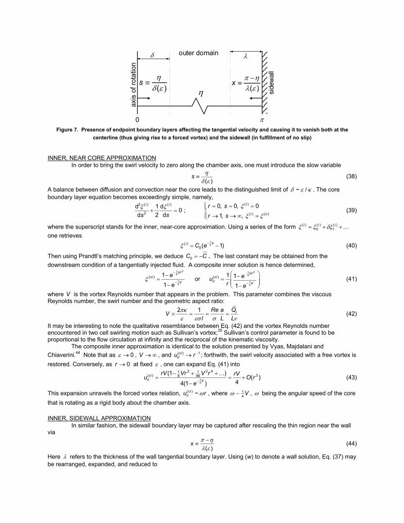
Figure 7. Presence of endpoint boundary layers affecting the tangential velocity and causing it to vanish both at the

centerline (thus giving rise to a forced vortex) and the sidewall (in fulfillment of no slip)

η

0 π

δ λ

axis

of r

otat

ion

outer domain

π ηλ ε−

≡( )

x ηδ ε

≡( )

s

side

wal

l

ξ ξπ⎛ ⎞+ − =⎜ ⎟⎝ ⎠

2 ( ) ( )2

2d 1 1 d1 0

2 6 dd

w w

xx;

ξ

ξ ξ

⎧ = = =⎪⎨

→ → ∞ =⎪⎩

( )

( ) ( )

1, 0, 00, ,

w

w ci

r xr x

(45)

where λ ε κ≡ / is taken to be the distinguished limit. Corresponding boundary conditions consist of the no slip at the wall and blending with the composite inner solution in the outer domain. Following similar ideas of matching, the sidewall approximation may be obtained,

π

πξ

− − −

− −

−=

−

2 21 14 6

21 14 6

( 1) (1 )( )

( 1)

1( )1

V rw

V

ere

or π

θ π

− − −

− −

⎡ ⎤−= ⎢ ⎥⎢ ⎥−⎣ ⎦

2 21 14 6

21 14 6

( 1) (1 )( )

( 1)

1 1

1

V rw

V

eur e

(46)

The validity of Eq. (46) is restricted to the region adjacent to the wall. As → 0r , the outer solution is regained.

COMPOSITE, UNIFORMLY VALID APPROXIMATION Using the classic ideas of composite expansions, a uniformly valid solution may be arrived at from the combination of wall and composite inner solutions. The result is

( )

π

θ

− − −−−

−−

⎧ ⎡ ⎤− − < <⎪ ⎢ ⎥⎣ ⎦= ⎨⎪ − =⎪⎩

2 22 1 114 64

214

( 1) (1 )1

1

1 ; 0

1 ; (tangential injection at entry)

V rVr

Vr

r e e z lu

r e z l (47)

The swirl velocity is hence made non-singular and adjusted to satisfy the no slip condition at the wall. Its behavior is illustrated in Figs. 8 and 9. Other important flow ingredients are summarized in Table 3. These include the forced core thickness, the maximum swirl velocity, the tangential wall boundary layer thickness, vorticity, pressure, the distance to the point where the radial pressure gradient is largest, and the swirling intensity. As shown in Fig. 8, the tangential component of the velocity starts from zero at the wall and then increases rapidly to merge with the outer flowfield within a characteristic distance δw . It continues to increase until reaching a maximum value that delimits the envelope inside of which viscous forces become dominant. After passing through this maximum θ max( )u , the swirl velocity depreciates, within a radius δc , until it reaches zero at the chamber axis.

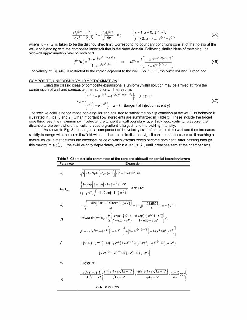
Table 3 Characteristic parameters of the core and sidewall tangential boundary layers Parameter Expression

δc ( )−⎡ ⎤− − − −⎢ ⎥⎣ ⎦1 12 21

22 1 2pln 1, / 2.24181/e V V

θ max( )u ( )

( ) ( )

−

−−

⎡ ⎤− + − −⎢ ⎥⎣ ⎦⎡ ⎤− − − −− ⎢ ⎥⎣ ⎦

12

12

11 24

1 12 2

12

1 exp pln 1,0.3191

1 2pln 1,1 V

e VV

ee

δw ( )αα

⎡ ⎤+ −⎣ ⎦− + − −144ln 0.01 0.99exp 28.56211 1 1 1

VV V

; α π= −216 1

Ω α α

π κ πα

⎧ ⎫− − −⎪ ⎪+ −⎨ ⎬− − − −⎪ ⎪⎩ ⎭

θ ze e2 21 1

2 2 4 41 14 4

exp( ) exp[ (1 )]4 sin( )2 1 exp( ) 1 exp( )

Vr V rVrz rV V

p

( )απ κ κ π

⎛ ⎞⎛ ⎞ − −−− ⎛ ⎞⎜ ⎟⎜ ⎟ ⎜ ⎟⎜ ⎟⎜ ⎟ ⎝ ⎠⎜ ⎟⎝ ⎠ ⎝ ⎠

⎡ ⎤− − − + − − +⎢ ⎥

⎢ ⎥⎣ ⎦

212144

22 12 2 2 2 2 2 210 22 1 1 1 sin

V rVrp z r e e r

( ) ( ) ( ) ( )α αα α α α− −⎡ ⎤+ − − − + −⎢ ⎥⎣ ⎦1 12 42 2 2 21 1 1 1 1

4 4 2 2 4Ei Ei Ei EiV VV Vr Vr e Vr e Vr

( ) ( )α αα α α− −⎡ ⎤− −⎢ ⎥⎣ ⎦1 14 41 1 1

4 2 4Ei EiV VVe e V V

δp 121.48351/V

Ω

π ππ πκ π π π

⎧ ⎫⎡ ⎤ ⎡ ⎤+ − + +− +⎪ ⎪⎣ ⎦ ⎣ ⎦− + −⎨ ⎬− +⎪ ⎪⎩ ⎭

1 14 4erf (1 ) 4 erfi (1 ) 4(1 ) 1 (1 ) (1)

4 2 4 4

i iV i iVi i Cz iV iV

(1) 0.779893C

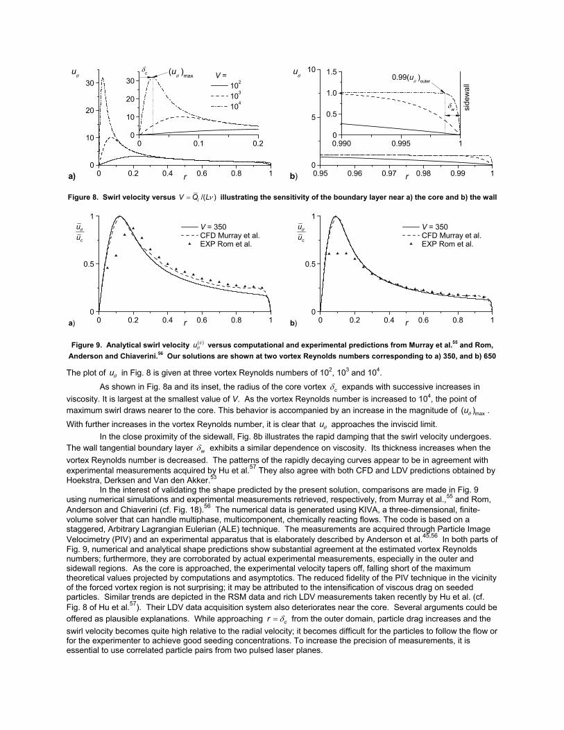
The plot of θu in Fig. 8 is given at three vortex Reynolds numbers of 102, 103 and 104.

As shown in Fig. 8a and its inset, the radius of the core vortex δc expands with successive increases in viscosity. It is largest at the smallest value of V. As the vortex Reynolds number is increased to 104, the point of maximum swirl draws nearer to the core. This behavior is accompanied by an increase in the magnitude of θ max( )u .

With further increases in the vortex Reynolds number, it is clear that θu approaches the inviscid limit. In the close proximity of the sidewall, Fig. 8b illustrates the rapid damping that the swirl velocity undergoes. The wall tangential boundary layer δw exhibits a similar dependence on viscosity. Its thickness increases when the vortex Reynolds number is decreased. The patterns of the rapidly decaying curves appear to be in agreement with experimental measurements acquired by Hu et al.57 They also agree with both CFD and LDV predictions obtained by Hoekstra, Derksen and Van den Akker.53 In the interest of validating the shape predicted by the present solution, comparisons are made in Fig. 9 using numerical simulations and experimental measurements retrieved, respectively, from Murray et al.,55 and Rom, Anderson and Chiaverini (cf. Fig. 18).56 The numerical data is generated using KIVA, a three-dimensional, finite-volume solver that can handle multiphase, multicomponent, chemically reacting flows. The code is based on a staggered, Arbitrary Lagrangian Eulerian (ALE) technique. The measurements are acquired through Particle Image Velocimetry (PIV) and an experimental apparatus that is elaborately described by Anderson et al.45,56 In both parts of Fig. 9, numerical and analytical shape predictions show substantial agreement at the estimated vortex Reynolds numbers; furthermore, they are corroborated by actual experimental measurements, especially in the outer and sidewall regions. As the core is approached, the experimental velocity tapers off, falling short of the maximum theoretical values projected by computations and asymptotics. The reduced fidelity of the PIV technique in the vicinity of the forced vortex region is not surprising; it may be attributed to the intensification of viscous drag on seeded particles. Similar trends are depicted in the RSM data and rich LDV measurements taken recently by Hu et al. (cf. Fig. 8 of Hu et al.57). Their LDV data acquisition system also deteriorates near the core. Several arguments could be offered as plausible explanations. While approaching δ= cr from the outer domain, particle drag increases and the swirl velocity becomes quite high relative to the radial velocity; it becomes difficult for the particles to follow the flow or for the experimenter to achieve good seeding concentrations. To increase the precision of measurements, it is essential to use correlated particle pairs from two pulsed laser planes.

0 0.2 0.4 0.6 0.8 10

10

20

30

0 0.1 0.20

10

20

30uθ V =

102

103

104

(uθ )max

δc

ra) 0.95 0.96 0.97 0.98 0.99 10

5

10

0.990 0.995 10

0.5

1.0

1.5uθ

r

0.99(uθ )outer

δw side

wal

l

b)

Figure 8. Swirl velocity versus ν= /( )iV Q L illustrating the sensitivity of the boundary layer near a) the core and b) the wall

0 0.2 0.4 0.6 0.8 10

0.5

1 θ

c

uu

r

V = 350 CFD Murray et al. EXP Rom et al.

a) 0 0.2 0.4 0.6 0.8 1

0

0.5

1 θ

c

uu

r

V = 350 CFD Murray et al. EXP Rom et al.

b)

Figure 9. Analytical swirl velocity θ( )cu versus computational and experimental predictions from Murray et al.55 and Rom,

Anderson and Chiaverini.56 Our solutions are shown at two vortex Reynolds numbers corresponding to a) 350, and b) 650

TOWARD A FULLY VISCOUS SOLUTION

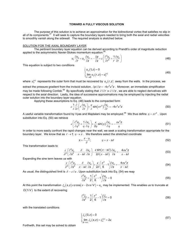
The purpose of this solution is to achieve an approximation for the bidirectional vortex that satisfies no slip in all of its components.47 It will seek to capture the boundary layers needed to bring both the axial and radial velocities to smoothly vanish along the sidewall. The required analysis is sketched below.

SOLUTION FOR THE AXIAL BOUNDARY LAYER The pertinent boundary layer equation can be derived according to Prandtl’s order of magnitude reduction applied to the axisymmetric Navier-Stokes momentum equation:58

ε⎛ ⎞∂ ∂ ∂ ∂∂

+ = − + +⎜ ⎟∂ ∂ ∂ ∂∂⎝ ⎠

2

21z z z z

r zu u u upu ur z z r rr

(48)

This equation is subject to two conditions

( )

( )→

⎧ =⎪⎨ =⎪⎩

( )

0

1, 0

lim ,z

oz z

r

u z

u r z u (49)

where ( )ozu represents the outer form that must be recovered by ( ),zu r z away from the walls. In the process, we

extract the pressure gradient from the inviscid solution, π κ∂ ∂ = − 2 2/ 4p z z . Moreover, an immediate simplification may be made following Conlisk.59 By specifically stating that ∂ ∂ ∂ ∂/ /r z , we are able to neglect derivatives with respect to the axial direction. Lastly, the idea of successive approximations may be employed by injecting the radial outer solution into the boundary layer equation. Applying these assumptions to Eq. (48) leads to the compacted form

( )κε π π κ∂ ∂∂ ⎛ ⎞ + = −⎜ ⎟∂ ∂ ∂⎝ ⎠2 2 21 sin 4z zu ur r z

r r r r r (50)

A useful variable transformation found by Vyas and Majdalani may be employed.46 We thus define η π= 2r . Upon substitution into Eq. (50) we retrieve

( )κ πκε ηη η η η ηη

⎛ ⎞∂ ∂ ∂+ + = −⎜ ⎟

∂ ∂∂⎝ ⎠

2 2

21 sin

2z z zu u u z (51)

In order to more easily confront the rapid changes near the wall, we seek a scaling transformation appropriate for the boundary layer. We know that as η π→ →1;r . We therefore select the stretched coordinate

π η η π δδ−

= = −;s s (52)

This transformation leads to

( )( )

κ π δε δ πκπ δ δ π δ π δδ

⎛ ⎞ −∂ ∂ ∂− − = −⎜ ⎟

− ∂ − ∂ −∂⎝ ⎠

2 2

2 2

sin 42

z z zsu u u zs s s s ss

(53)

Expanding the sine term leaves us with

ε δ κ π πκπ δ δ π δδ

⎛ ⎞ ⎛ ⎞∂ ∂ ∂− + − = −⎜ ⎟ ⎜ ⎟

− ∂ ∂ −∂ ⎝ ⎠⎝ ⎠

2 2 2

2 241

2 6z z zu u u z

s s s ss (54)

As usual, the distinguished limit is δ ε κ∼ / . Upon substitution back into Eq. (54) we reap

π⎛ ⎞∂ ∂+ − =⎜ ⎟

∂∂ ⎝ ⎠

2 2

21 1 02 6

z zu uss

(55)

At this point the transformation ( ) ( )ξ π π π− =, cos 2 /z zs z z s V u may be implemented. This enables us to truncate at

( )1/O V to the extent of recovering

ξ ξπ⎛ ⎞∂ ∂+ − =⎜ ⎟

∂∂ ⎝ ⎠

2 2

21 1 02 6

z z

ss (56)

with the translated conditions

( )

( )ξ

ξ ξ κ→∞

⎧ =⎪⎨ = =⎪⎩

( )

0, 0

lim , 2z

oz zs

z

s z (57)

Forthwith, this set may be solved to obtain

( ) ξ κ π⎡ ⎤= − − −⎣ ⎦21 1

2 62 1 exp 1z s (58)

Rewriting Eq. (58) in terms of the unscaled variables renders the final solution. We get

( ) ππκ π − − −⎡ ⎤= −⎢ ⎥⎣ ⎦

2 21 14 6( 1) (1 )22 cos 1 V r

zu z r e (59)

where πκ ε= 2 /V is the same vortex Reynolds number expressed by Eq. (42). We also note the symmetry between the axial boundary layer correction and that realized for the swirl velocity at the wall.

SOLUTION FOR THE RADIAL BOUNDARY LAYER Corrections of this nature are typically disregarded when the inviscid velocity vanishes at the wall; however viscosity has a tempering effect on the curvature of the radial profile that is investigated here. The reduction of the Navier-Stokes equations is more subtle because the viscous correction could be considered to be secondary. While Prandtl’s method still applies, one must retain terms to the second order lest a meaningless outcome is engendered. The process requires starting with

θε⎛ ⎞∂ ∂ ∂ ∂ ∂

+ − − + − =⎜ ⎟∂ ∂ ∂ ∂∂⎝ ⎠

22

2 21r r r r r

r zuu u u u u pu u

r r r r z rr r (60)

which is subject to

( )

( )→

⎧ =⎪⎨ =⎪⎩

( )

0

1 0

limr

or r

r

u

u r u (61)

By assuming that radial changes are more significant than axial ones, we eliminate all axial derivatives and take the pressure gradient calculated from the inviscid solution,37

( ) ( )κ π π π∂ ⎡ ⎤= − +⎣ ⎦∂

22 2 3 2

3 31sin 1 2 cotp r r r

r r r (62)

We recognize that this term is ( )κ 2O near the wall due to some cancellation with the θ2 /u r term. Then just as

before, we inject the inviscid solution into the boundary layer equation. Rewriting Eq. (60) gives

( ) ( ) ( )κ κ κε π π π⎡ ⎤⎡ ⎤⎛ ⎞ + + = ⎢ ⎥⎢ ⎥⎜ ⎟

⎝ ⎠⎣ ⎦ ⎣ ⎦

22 2 2 2

3 3d d1 d sin sin sin

d d dr ru ur r r O r

r r r r rr r (63)

The transformation η π= 2r follows. With careful substitution and factorization of Eq. (63), we get

( ) ( ) ( )κ π κ κε η η πη η η ηη η

⎡ ⎤ ⎡ ⎤+ + + =⎢ ⎥ ⎢ ⎥

⎢ ⎥ ⎣ ⎦⎣ ⎦

2 22 2

2 5 / 2 3d d d1 sin sin sin

d 2 dd 4r r ru u u O r

r (64)

The sidewall variable transformation ( )π η δ= − /s can thus be applied along with the sine expansion; the radial equation becomes

( )

( )ε δ δ κ π κ ππ δπ δ δδ π δ

⎡ ⎤ ⎛ ⎞⎢ ⎥− + − + − ≈⎜ ⎟

−⎢ ⎥− ⎝ ⎠⎣ ⎦

2 2 2

2 2 5 / 2d d dsin 1 0

d 2 6 dd 4r r ru u us

s s ss s (65)

where δ ε κ∼ / re-emerges. Reinserting the distinguished limit into Eq. (65) we can reveal the following form

π⎛ ⎞+ − =⎜ ⎟

⎝ ⎠

2 2

2d d1 1 0

2 6 ddr ru u

ss (66)

As with the axial case we introduce ξ π= 2/ sin( )r rru r and proceed to seek a solution in the same manner. Boundary conditions follow, namely,

( )

( )ξ

ξ ξ κ→∞

⎧ =⎪⎨ = = −⎪⎩

(0)

0 0

limr

r rss

(67)

The solution is readily found to be

( ) πκ π − − −⎡ ⎤= − −⎢ ⎥⎣ ⎦

2 21 12 6( 1) (1 )2sin 1 V r

ru r er

(68)

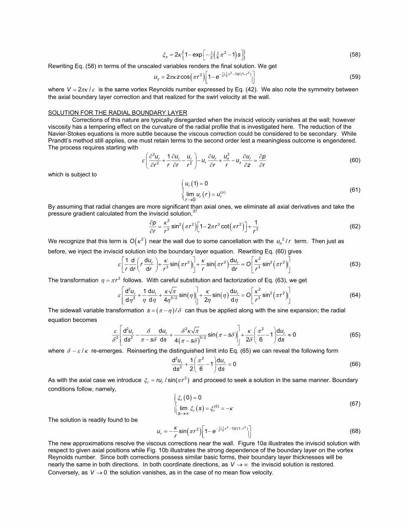
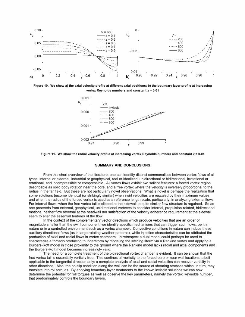
The new approximations resolve the viscous corrections near the wall. Figure 10a illustrates the inviscid solution with respect to given axial positions while Fig. 10b illustrates the strong dependence of the boundary layer on the vortex Reynolds number. Since both corrections possess similar basic forms, their boundary layer thicknesses will be nearly the same in both directions. In both coordinate directions, as →∞V the inviscid solution is restored. Conversely, as → 0V the solution vanishes, as in the case of no mean flow velocity.

SUMMARY AND CONCLUSIONS

From this short overview of the literature, one can identify distinct commonalities between vortex flows of all types: internal or external, industrial or geophysical, real or idealized, unidirectional or bidirectional, irrotational or rotational, and incompressible or compressible. All vortex flows exhibit two salient features: a forced vortex region describable as solid body rotation near the core, and a free vortex where the velocity is inversely proportional to the radius in the far field. But these are not particularly novel observations. What is novel is perhaps the realization that some solutions become identical (or strikingly similar) when swirl velocities are rescaled by their maximum values and when the radius of the forced vortex is used as a reference length scale, particularly, in analyzing external flows. For internal flows, when the free vortex tail is clipped at the sidewall, a quite similar flow structure is regained. So as one proceeds from external, geophysical, unidirectional vortexes to consider internal, propulsion-related, bidirectional motions, neither flow reversal at the headwall nor satisfaction of the velocity adherence requirement at the sidewall seem to alter the essential features of the flow. In the context of the complementary vector directions which produce velocities that are an order of magnitude smaller than the swirl component, we identify specific mechanisms that can trigger such flows, be it in nature or in a controlled environment such as a vortex chamber. Convective conditions in nature can induce these auxiliary directional flows (as in large rotating weather patterns), while injection characteristics can be attributed the production of axial and radial flows in vortex chambers. In retrospect a dual model could perhaps be used to characterize a tornado producing thunderstorm by modeling the swirling storm via a Rankine vortex and applying a Burgers-Rott model in close proximity to the ground where the Rankine model lacks radial and axial components and the Burgers-Rott model becomes increasingly valid. The need for a complete treatment of the bidirectional vortex chamber is evident. It can be shown that the free vortex tail is essentially vorticity free. This confines all vorticity to the forced core or near wall locations, albeit applicable to the tangential direction only: a complete analysis of axial and radial velocities can recover vorticity in other directions. Also, the no slip condition along the wall can be the source of shearing stresses which, in turn, may translate into roll torques. By applying boundary layer treatments to the known inviscid solutions we can now determine the potential for roll torques as well as observe the key parameters, namely the vortex Reynolds number, that predominately controls the boundary layers.

0 0.2 0.4 0.6 0.8 1

-0.05

0.00

0.05

0.10

a)

r

V = 650 z = 0.1 z = 0.3 z = 0.5 z = 0.7 z = 0.9

uz

0.90 0.92 0.94 0.96 0.98 1

-0.04

-0.02

0

b)

uz

r

V = 200 400 600 800

Figure 10. We show a) the axial velocity profile at different axial positions; b) the boundary layer profile at increasing vortex Reynolds numbers and constant κ = 0.01

0.97 0.98 0.99 1-0.002

-0.001

0.000

0.001ur

r

V = inviscid 200 400 600 800

Figure 11. We show the radial velocity profile at increasing vortex Reynolds numbers and constant κ = 0.01

FUTURE WORK

There are a number of additional challenges that have yet to be met. A more comprehensive model for the bidirectional vortex is our goal. In typical vortex chambers such as centrifugal separators, it is often acceptable to assume incompressible conditions because of the small mass flow rate and/or low maximum velocities. However, in terms of propulsion applications, compressibility can have an appreciable effect. Typical injection velocities can approach Mach numbers where the onset of compressibility is imminent. In reactive vortex chambers, a compressible treatment is required to handle the combustion region inside the mantle where the expanding gasses are trapped. Under these auspices, leading order inviscid approximations become unsuitable as initial solutions because of their singularities near the axis of rotation. A quasi viscous leading order solution in the swirl direction will be needed at the foundation of a compressible flow analysis. Uniting the work done in determining the viscous boundary layers along the walls and corners of the chamber to the compressible solution will provide an even more accurate platform for stability prediction and analysis. The relaxation of the limiting assumptions also constitutes a vital area of interest for further studies. Finding a vortex model that is not dependent on the isentropic flow condition is an intriguing area that must be undertaken in the process of paving the way for a successful thermal analysis of the combustion chamber. A solution that does not neglect the axial variations of the swirl velocity is also of particular interest. Of course, as the characterization of the bidirectional vortex evolves so do the complications in the treatment. Several interesting geometric configurations still need to be considered and the problem of a compressible, thermally sensitive model of a confined cyclone remains at large.

ACKNOWLEDGMENTS

The authors are deeply grateful for the support received from ORBITEC (FA8650-05-C-2612) and the National Science Foundation (CMS-0353518). We also appreciate the institutional cost sharing received from the University of Tennessee Space Institute. The support and encouragement of both Dr. Martin J. Chiaverini and Dr. Richard Cohn, the ORBITEC and AFRL/PRS technical monitors, are most gratefully acknowledged.

REFERENCES

1. Penner, S. S., "Elementary Considerations of the Fluid Mechanics of Tornadoes and Hurricanes," Acta Astronautica, Vol. 17, pp. 351-362 (1972).

2. Königl, A., "Stellar and Galactic Jets: Theoretical Issues," Canadian Journal of Physics, Vol. 64, pp. 362-368 (1986).

3. Kirshner, R. P., The Extravagant Universe: Exploding Stars, Dark Energy, and the Accelerating Cosmos, Princeton University Press, Princeton, New Jersey (2004).

4. Reydon, R. F., and Gauvin, W. H., "Theoretical and Experimental Studies of Confined Vortex Flow," The Canadian Journal of Chemical Engineering, Vol. 59, pp. 14-23 (1981).

5. Chiaverini, M. J., Malecki, M. J., Sauer, J. A., Knuth, W. H., and Majdalani, J., “Vortex Thrust Chamber Testing and Analysis for O2-H2 Propulsion Applications,” AIAA Paper 2003-4473 (July 2003).

6. Chiaverini, M. J., Malecki, M. M., Sauer, J. A., Knuth, W. H., and Hall, C. D., “Testing and Evaluation of Vortex Combustion Chamber for Liquid Rocket Engines,” JANNAF (April 2002).

7. Chiaverini, M. J., Malecki, M. J., Sauer, J. A., and Knuth, W. H., “Vortex Combustion Chamber Development for Future Liquid Rocket Engine Applications,” AIAA Paper 2002-2149 (July 2002).

8. Vyas, A. B., Majdalani, J., and Chiaverini, M. J., “The Bidirectional Vortex. Part 3: Multiple Solutions,” AIAA Paper 2003-5054 (July 2003).

9. Harvey, J. K., "Some Observations of the Vortex Breakdown Phenomenon," Journal of Fluid Mechanics, Vol. 14, No. 4, pp. 585-592 (1962).

10. Sarpkaya, T., "On Stationary and Travelling Vortex Breakdowns," Journal of Fluid Mechanics, Vol. 45, No. 3, pp. 545-559 (1971).

11. Leibovich, S., "The Structure of Vortex Breakdown," Annual Review of Fluid Mechanics, Vol. 10, pp. 221-246 (1978).

12. Leibovich, S., "Vortex Stability and Breakdown: Survey and Extension," AIAA Journal, Vol. 22, No. 9, pp. 1192-1206 (1984).

13. Lilley, D. G., "Swirl Flows in Combustion: A Review," AIAA Journal, Vol. 15, No. 8, pp. 1063-1078 (1977). 14. Gupta, A. K., Lilley, D. G., and Syred, N., Swirl Flows, Abacus, London, UK (1984). 15. Durbin, M. D., Vangsness, M. D., Ballal, D. R., and Katta, V. R., "Study of Flame Stability in a Step-Swirl

Combustor," Journal of Engineering for Gas Turbines and Power-Transactions of the ASME, Vol. 118, pp. 308-314 (1996).

16. Lewellen, W. S., A Review of Confined Vortex Flows, NASA, Technical Rept. CR-1772 (July 1971). 17. Vatistas, G. H., Lin, S., and Kwok, C. K., "Theoretical and Experimental Studies on Vortex Chamber Flows," AIAA

Journal, Vol. 24, No. 4, pp. 635-642 (1986). 18. Vatistas, G. H., Lin, S., and Kwok, C. K., "Reverse Flow Radius in Vortex Chambers," AIAA Journal, Vol. 24, No.

11, pp. 1872-1873 (1986).

19. Vatistas, G. H., Jawarneh, A. M., and Hong, H., "Flow Characteristics in a Vortex Chamber," The Canadian Journal of Chemical Engineering, Vol. 83, No. 6, pp. 425-436 (2005).

20. Flinn, E. D., Cooling of a Hot New Engine, in Aerospace America 39, pp. 26-27 (2001). 21. Rankine, W. J. M., A Manual of Applied Mechanics, 9th ed., C. Griffin and Co., London, UK (1858). 22. Brown, R. A., Flikinger, B. A., Gorren, E., Schultz, D. M., Sirmans, D., Spencer, P. L., Wood, V. T., and Ziegler, C.

L., "Improved Detection of Severe Storms Using Experimental Fine Resolution Wrs-88d Measurements," Weather Forcasting, Vol. 20, pp. 3-14 (2005).

23. Mallen, K. J., Montgomery, M. T., and Wang, B., "Reexamining the near-Core Radial Structure of the Tropical Cyclone Primary Circulation: Implications for Vortex Resiliency," Journal of the Atmospheric Sciences, Vol. 62, No. 2, pp. 408-425 (2005).

24. Bertato, M., Giaiotti, D. B., Mansato, A., and Stel, F., "An Interesting Case of Tornado in Friuli-Northeastern Italy.," Atomospheric Research, Vol. 7-68, pp. 3-21 (2003).

25. Wendt, B. J., Initial Circulation and Peak Vorticity Behavior of Vortices Shed from Airfoil Vortex Generators, NASA, Technical Rept. NASA/CR—2001-211144 (August 2001).

26. Alekseenko, S. V., Kuibin, P. A., Okulov, V. L., and Shtork, S. I., "Helical Vortices in Swirl Flow," Journal of Fluid Mechanics, Vol. 382, No. 1, pp. 195-243 (1999).

27. Batchelor, G. K., "Axial Flow in Trailing Line Vortices," Journal of Fluid Mechanics, Vol. 20, No. 4, pp. 645-658 (1964).

28. Schmid, P. J., and Rossi, M., "Three-Dimensional Stability of a Burgers Vortex," Journal of Fluid Mechanics, Vol. 500, No. 1, pp. 103-112 (2004).

29. Pérez-Saborid, M., Herrada, M. A., Gómez-Barea, A., and Barrero, A., "Downstream Evolution of Unconfined Vortices: Mechanical and Thermal Aspects," Journal of Fluid Mechanics, Vol. 471, No. 1, pp. 51-70 (2002).

30. Eloy, C., and Le Dizès, S., "Three-Dimensional Instability of Burgers and Lamb-Oseen Vortices in a Strain Field," Journal of Fluid Mechanics, Vol. 378, No. 1, pp. 145-166 (1999).

31. Devenport, W. J., Rife, M. C., Liapis, S. I., and Follin, G. J., "The Structure and Development of a Wing-Tip Vortex," Journal of Fluid Mechanics, Vol. 312, No. 1, pp. 67-106 (1996).

32. Faler, J. H., and Leibovich, S., "Disrupted States of Vortex Flow and Vortex Breakdown," Physics of Fluids, Vol. 20, No. 9, pp. 1385-1400 (1977).

33. Escudier, M. P., "Vortex Breakdown - Observations and Explanations," Progress in Aerospace Sciences, Vol. 25, No. 2, pp. 189-229 (1988).

34. Long, R. R., "A Vortex in an Infinite Viscous Fluid," Journal of Fluid Mechanics, Vol. 11, No. 4, pp. 611-624 (1961). 35. Sullivan, R. D., "A Two-Cell Vortex Solution of the Navier-Stokes Equations," Journal of the Aerospace Sciences,

Vol. 26, pp. 767-768 (1959). 36. Bloor, M. I. G., and Ingham, D. B., "The Flow in Industrial Cyclones," Journal of Fluid Mechanics, Vol. 178, No. 1,

pp. 507-519 (1987). 37. Vyas, A. B., and Majdalani, J., "Exact Solution of the Bidirectional Vortex," AIAA Journal, Vol. 44, No. 10, pp. 2208-

2216 (2006). 38. Wu, J. Z., "Conical Turbulent Swirling Vortex with Variable Eddy Viscosity," Proceedings of the Royal Society, Vol.

403, No. 1825, pp. 235-268 (1986). 39. Nolan, D. S., and Farrell, B. F., "Generalized Stability Analyses of Asymmetric Disturbances in One- and Two-

Celled Vorticies Maintained by Radial Inflow," Journal of the Atmospheric Sciences, Vol. 56, pp. 1282-1307 (1999). 40. Bloor, M. I. G., and Ingham, D. B., "Theoretical Investigation of the Flow in a Conical Hydrocyclone," Transactions

of the Institution of Chemical Engineers, Vol. 51, No. 1, pp. 36-41 (1973). 41. Kelsall, D. F., "A Study of Motion of Solid Particles in a Hydraulic Cyclone," Transactions of the Institution of

Chemical Engineers, Vol. 30, pp. 87-103 (1952). 42. Vyas, A. B., Majdalani, J., and Chiaverini, M. J., “The Bidirectional Vortex. Part 1: An Exact Inviscid Solution,” AIAA

Paper 2003-5052 (July 2003). 43. Majdalani, J., and Rienstra, S. W., "On the Bidirectional Vortex and Other Similarity Solutions in Spherical

Coordinates," Journal of Applied Mathematics and Physics (ZAMP), Vol. 58, No. 2, pp. 289-308 (2007). 44. Vyas, A. B., Majdalani, J., and Chiaverini, M. J., “The Bidirectional Vortex. Part 2: Viscous Core Corrections,” AIAA

Paper 2003-5053 (July 2003). 45. Anderson, M. H., Valenzuela, R., Rom, C. J., Bonazza, R., and Chiaverini, M. J., “Vortex Chamber Flow Field

Characterization for Gelled Propellant Combustor Applications,” AIAA Paper 2003-4474 (July 2003). 46. Vyas, A. B., and Majdalani, J., “Characterization of the Tangential Boundary Layers in the Bidirectional Vortex

Thrust Chamber,” AIAA Paper 2006-4888 (July 2006). 47. Batterson, J. W., and Majdalani, J., “On the Boundary Layers of the Bidirectional Vortex ” AIAA Paper 2007-4123

(June 2007). 48. Maicke, B. A., and Majdalani, J., “The Compressible Bidirectional Vortex ” AIAA Paper 2007-4122 (June 2007). 49. Majdalani, J., "On Steady Rotational High Speed Flows: The Compressible Taylor-Culick Profile," Proceedings of

the Royal Society, Series A, Vol. 463, No. 2077, pp. 131-162 (2007). 50. Majdalani, J., “The Compressible Taylor-Culick Flow,” AIAA Paper 2005-3542 (July 2005). 51. Maicke, B. A., and Majdalani, J., “The Compressible Taylor Flow in Slab Rocket Motors,” AIAA Paper 2006-4957

(July 2006). 52. Smith, J. L., "An Analysis of the Vortex Flow in the Cyclone Separator," Journal of Basic Engineering-Transactions

of the ASME, pp. 609-618 (1962).

53. Hoekstra, A. J., Derksen, J. J., and Van den Akker, H. E. A., "An Experimental and Numerical Study of Turbulent Swirling Flow in Gas Cyclones," Chemical Engineering Science, Vol. 54, No. 13, pp. 2055-2065 (1999).

54. Balachandar, S., Buckmaster, J. D., and Short, M., "The Generation of Axial Vorticity in Solid-Propellant Rocket-Motor Flows," Journal of Fluid Mechanics, Vol. 429, No. 1, pp. 283-305 (2001).

55. Murray, A. L., Gudgen, A. J., Chiaverini, M. J., Sauer, J. A., and Knuth, W. H., “Numerical Code Development for Simulating Gel Propellant Combustion Processes,” JANNAF (May 2004).

56. Rom, C. J., Anderson, M. H., and Chiaverini, M. J., “Cold Flow Analysis of a Vortex Chamber Engine for Gelled Propellant Combustor Applications,” AIAA Paper 2004-3359 (July 2004).

57. Hu, L. Y., Zhou, L. X., Zhang, J., and Shi, M. X., "Studies of Strongly Swirling Flows in the Full Space of a Volute Cyclone Separator," AIChE Journal, Vol. 51, No. 3, pp. 740-749 (2005).

58. Prandtl, L., "Zur Berechnung Der Grenzschichten," ZAMM, No. 18, pp. 77-82 (1938). 59. Conlisk, A. T., Source-Sink Flows in a Rapidly Rotating Annulus, Dissertation, Purdue (1978).