Embed Size (px)
DESCRIPTION
best slide to lear advanced quality control
Citation preview

1
IEE 570 Advanced Quality Control
Instructor: Jing Li
Lecture notes #3
2
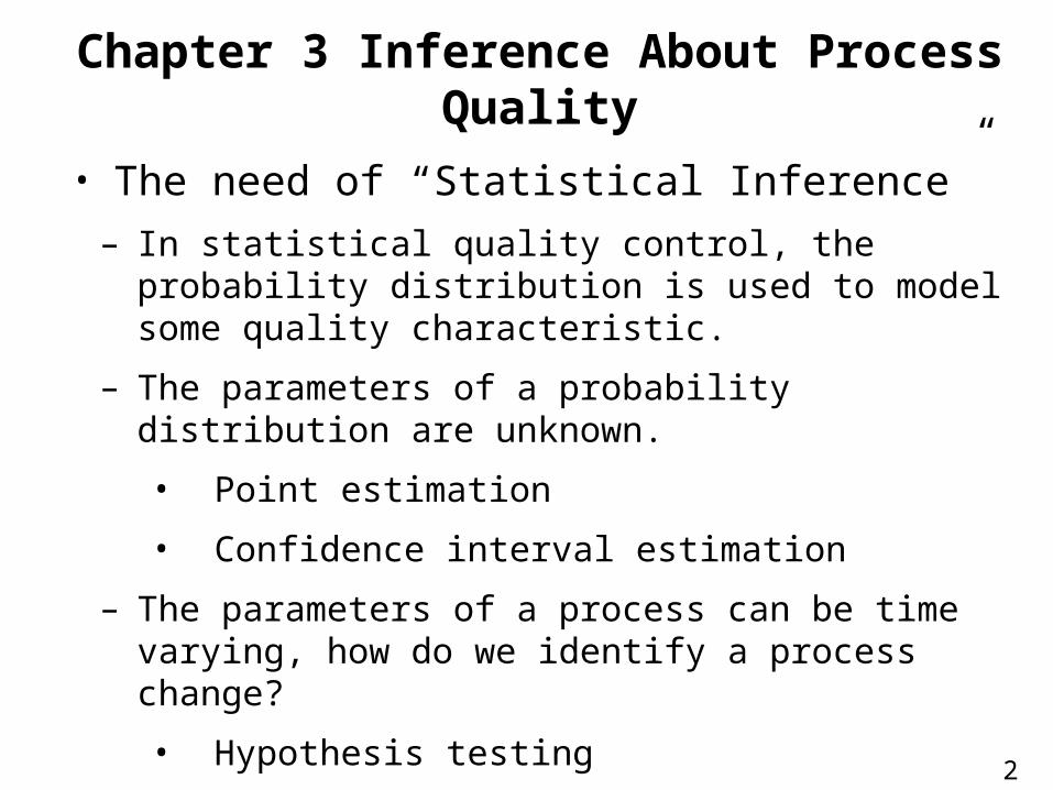
• The need of “Statistical Inference”
– In statistical quality control, the probability distribution is used to model some quality characteristic.
– The parameters of a probability distribution are unknown.
• Point estimation
• Confidence interval estimation
– The parameters of a process can be time varying, how do we identify a process change?
• Hypothesis testing
Chapter 3 Inference About Process Quality
3
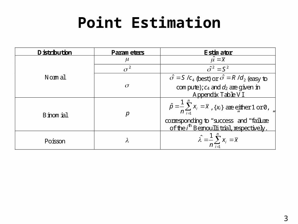
Point Estimation
Distribution Parameters Estimator x̂
2 22ˆ S Normal
4/ˆ cS (best) or 2/ˆ dR (easy to
compute); c4 and d2 are given in Appendix Table VI
Binomial p xx
np
n
ii
1
1ˆ , {xi} are either 1 or 0,
corresponding to “success” and “failure” of the ith Bernoulli trial, respectively.
Poisson xxn
n
ii
1
1̂
4
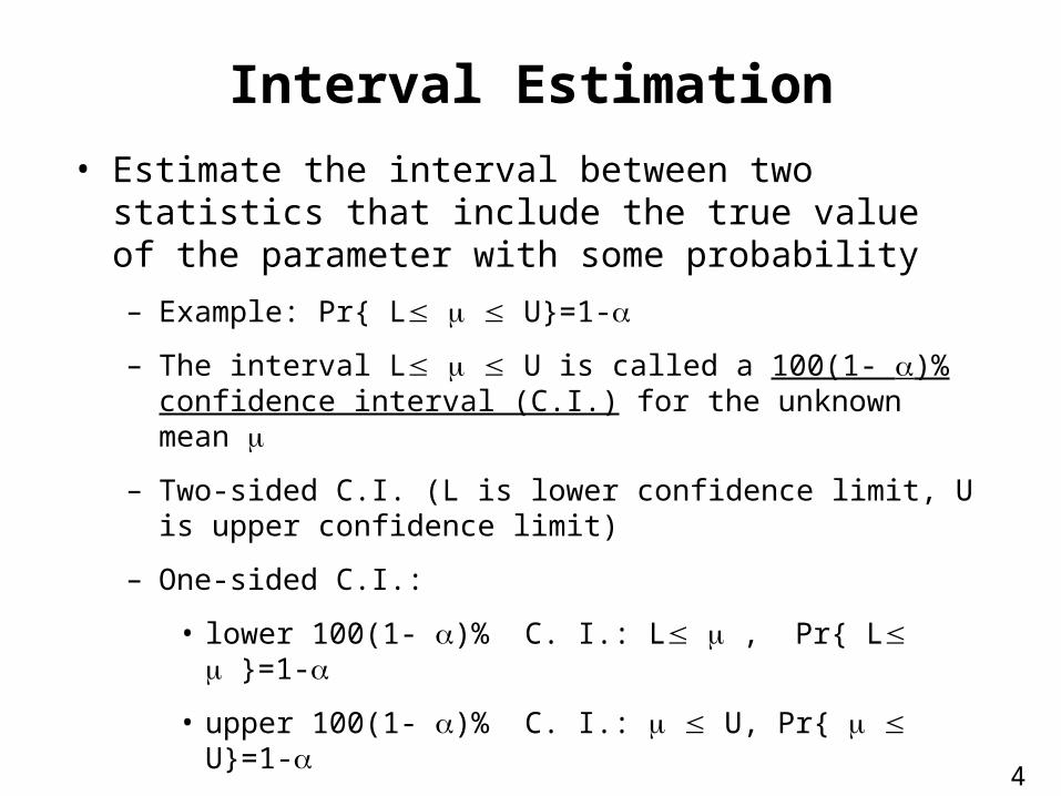
Interval Estimation
• Estimate the interval between two statistics that include the true value of the parameter with some probability
– Example: Pr{ L U}=1-
– The interval L U is called a 100(1- )% confidence interval (C.I.) for the unknown mean
– Two-sided C.I. (L is lower confidence limit, U is upper confidence limit)
– One-sided C.I.:
• lower 100(1- )% C. I.: L , Pr{ L }=1-
• upper 100(1- )% C. I.: U, Pr{ U}=1-
5
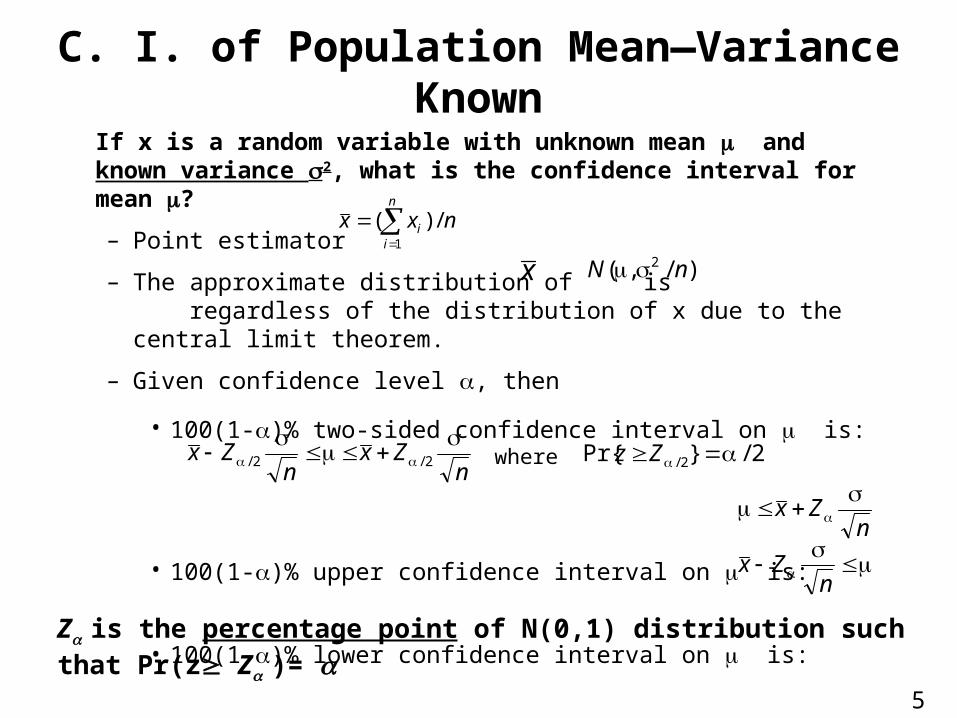
If x is a random variable with unknown mean and known variance 2, what is the confidence interval for mean ?
– Point estimator
– The approximate distribution of is regardless of the distribution of x due to the central limit theorem.
– Given confidence level , then
• 100(1-)% two-sided confidence interval on is:
• 100(1-)% upper confidence interval on is:
• 100(1-)% lower confidence interval on is:
n
ii nxx
1
/)(
)/,( 2 nN
nZx
nZx
2/2/ 2/}Pr{ 2/ Zzwhere
nZx
n
Zx
x
Z is the percentage point of N(0,1) distribution such that Pr(z Z )=
C. I. of Population Mean—Variance Known
6
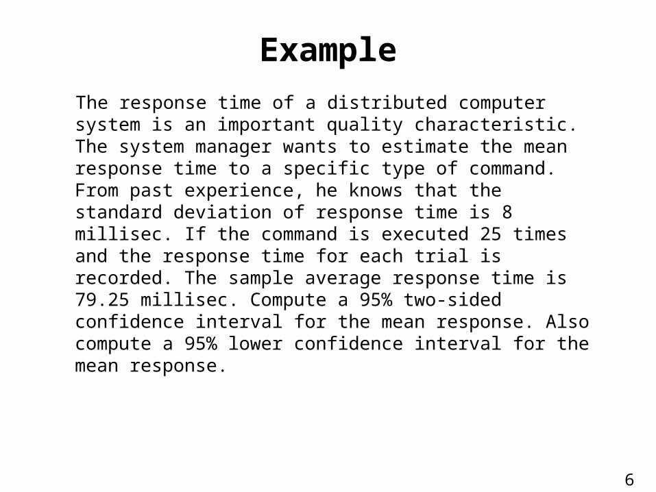
The response time of a distributed computer system is an important quality characteristic. The system manager wants to estimate the mean response time to a specific type of command. From past experience, he knows that the standard deviation of response time is 8 millisec. If the command is executed 25 times and the response time for each trial is recorded. The sample average response time is 79.25 millisec. Compute a 95% two-sided confidence interval for the mean response. Also compute a 95% lower confidence interval for the mean response.
Example
7
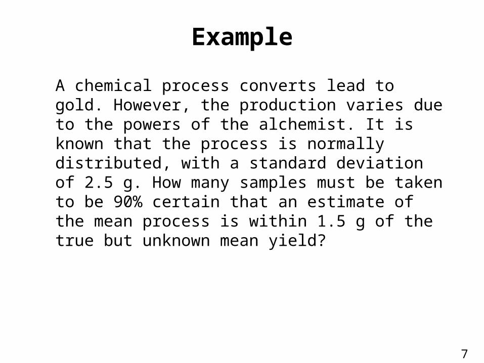
A chemical process converts lead to gold. However, the production varies due to the powers of the alchemist. It is known that the process is normally distributed, with a standard deviation of 2.5 g. How many samples must be taken to be 90% certain that an estimate of the mean process is within 1.5 g of the true but unknown mean yield?
Example
8
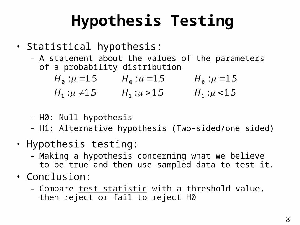
Hypothesis Testing
• Statistical hypothesis:– A statement about the values of the parameters of a probability
distribution
– H0: Null hypothesis– H1: Alternative hypothesis (Two-sided/one sided)
• Hypothesis testing:– Making a hypothesis concerning what we believe to be true and
then use sampled data to test it.
• Conclusion:– Compare test statistic with a threshold value, then reject or fail
to reject H0
5.1:
5.1:
1
0
H
H
5.1:
5.1:
1
0
H
H
5.1:
5.1:
1
0
H
H
9
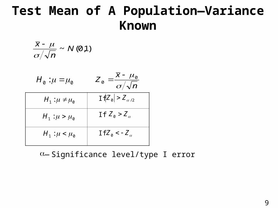
Test Mean of A Population—Variance Known
— Significance level/type I error
)1,0(~ Nn
x
00 : H
If
If
If
01 : H
n
xZ
0
0
2/0 ZZ
ZZ 0
ZZ 0
01 : H
01 : H
10
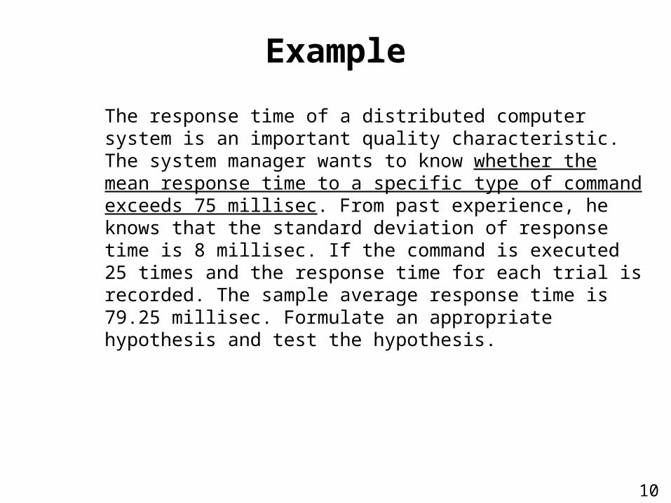
Example
The response time of a distributed computer system is an important quality characteristic. The system manager wants to know whether the mean response time to a specific type of command exceeds 75 millisec. From past experience, he knows that the standard deviation of response time is 8 millisec. If the command is executed 25 times and the response time for each trial is recorded. The sample average response time is 79.25 millisec. Formulate an appropriate hypothesis and test the hypothesis.
11
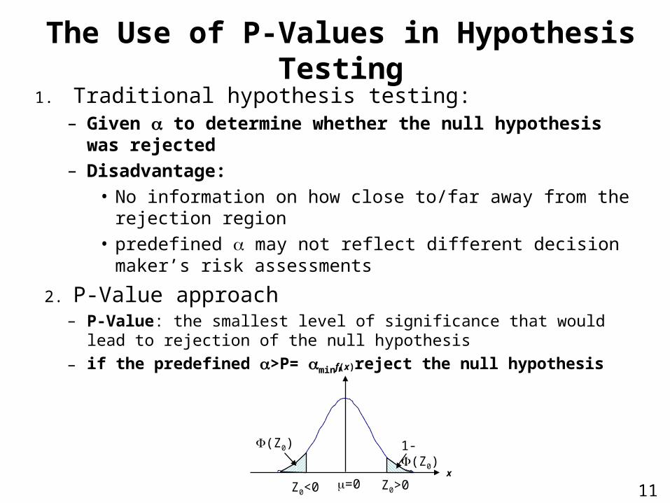
1. Traditional hypothesis testing:– Given to determine whether the null hypothesis was
rejected– Disadvantage:
• No information on how close to/far away from the rejection region
• predefined may not reflect different decision maker’s risk assessments
2. P-Value approach– P-Value: the smallest level of significance that would lead to rejection of
the null hypothesis
– if the predefined >P= min, reject the null hypothesisf(x)
x=0 Z0>0Z0<0
1-(Z0)(Z0)
The Use of P-Values in Hypothesis Testing
12
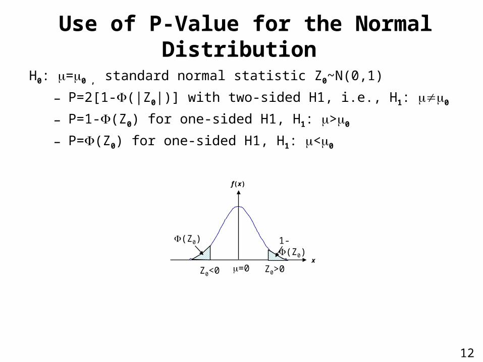
Use of P-Value for the Normal Distribution
H0: =0 , standard normal statistic Z0~N(0,1)
– P=2[1-(|Z0|)] with two-sided H1, i.e., H1: 0
– P=1-(Z0) for one-sided H1, H1: >0
– P=(Z0) for one-sided H1, H1: <0
f(x)
x=0 Z0>0Z0<0
1-(Z0)(Z0)
13
Example (Revisit)
The response time of a distributed computer system is an important quality characteristic. The system manager wants to know whether the mean response time to a specific type of command exceeds 75 millisec. From past experience, he knows that the standard deviation of response time is 8 millisec. If the command is executed 25 times and the response time for each trial is recorded. The sample average response time is 79.25 millisec. Formulate an appropriate hypothesis and test the hypothesis. Compute the P-value.
14
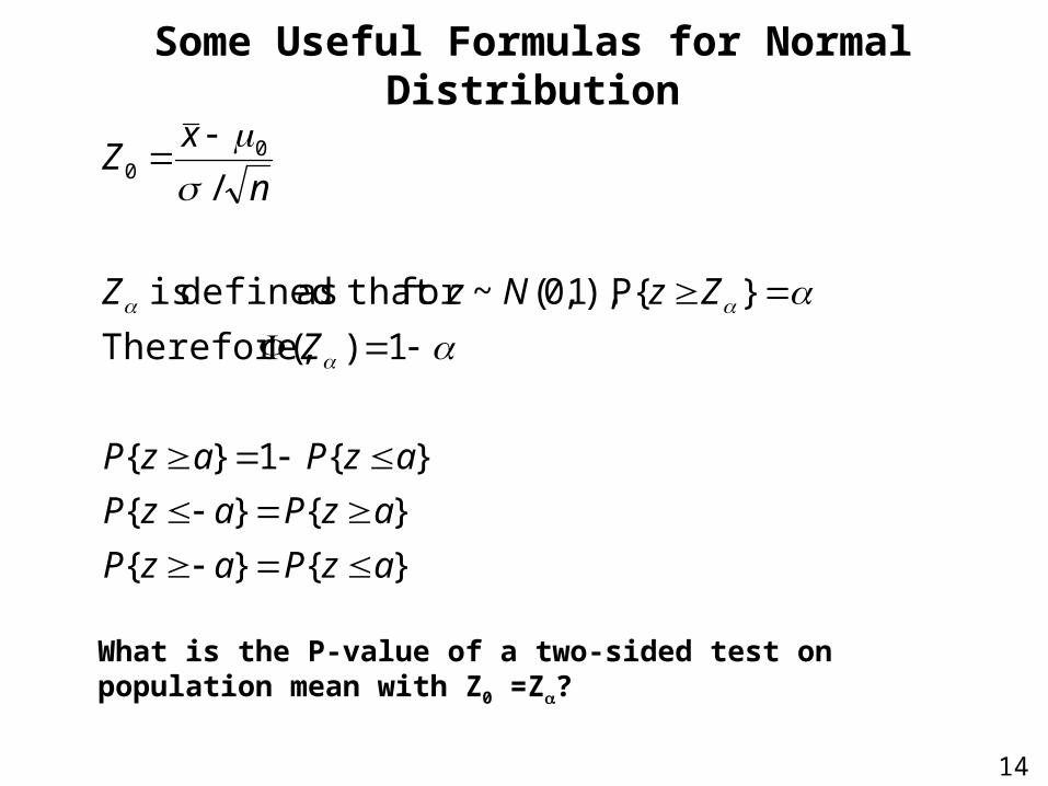
Some Useful Formulas for Normal Distribution
}{}{
}{}{
}{1}{
1)( Therefore,
}P{),1,0(~for that as defined is
/0
0
azPazP
azPazP
azPazP
Z
ZzNzZ
n
xZ
What is the P-value of a two-sided test on population mean with Z0 =Z?
15
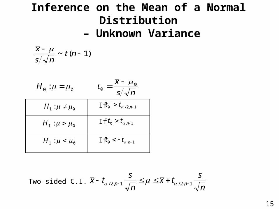
Inference on the Mean of a Normal Distribution – Unknown Variance
n
stx
n
stx nn 1,2/1,2/
)1(~
ntns
x
00 : H
If
If
If
01 : H
ns
xt 0
0
1,2/0 ntt
1,0 ntt
1,0 ntt
01 : H
01 : H
Two-sided C.I.
16
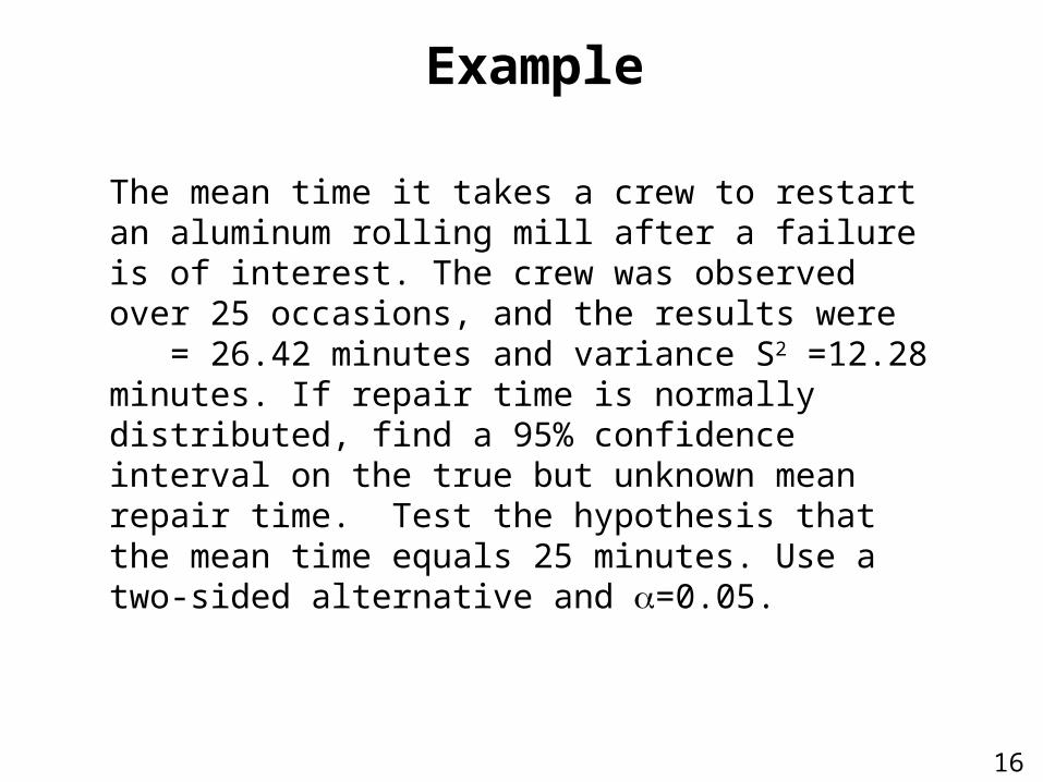
The mean time it takes a crew to restart an aluminum rolling mill after a failure is of interest. The crew was observed over 25 occasions, and the results were = 26.42 minutes and variance S2 =12.28 minutes. If repair time is normally distributed, find a 95% confidence interval on the true but unknown mean repair time. Test the hypothesis that the mean time equals 25 minutes. Use a two-sided alternative and =0.05.
Example
17
• If the value of the parameter specified by the null hypothesis is contained in the 100(1- )% interval, then the null hypothesis cannot be rejected at the level.
• If the value specified by the null hypothesis is not in the interval, then the null hypothesis can be rejected at the level
Confidence Interval and Hypothesis Testing
18
Understanding the result of Hypothesis Test
• When we reject the null hypothesis, it is a strong conclusion: there is a strong evidence that the null hypothesis is false.
• When we fail to reject the null hypothesis, it is a weak conclusion: It does not mean that the null hypothesis is correct. It only means we do not have strong evidence to reject it.
19
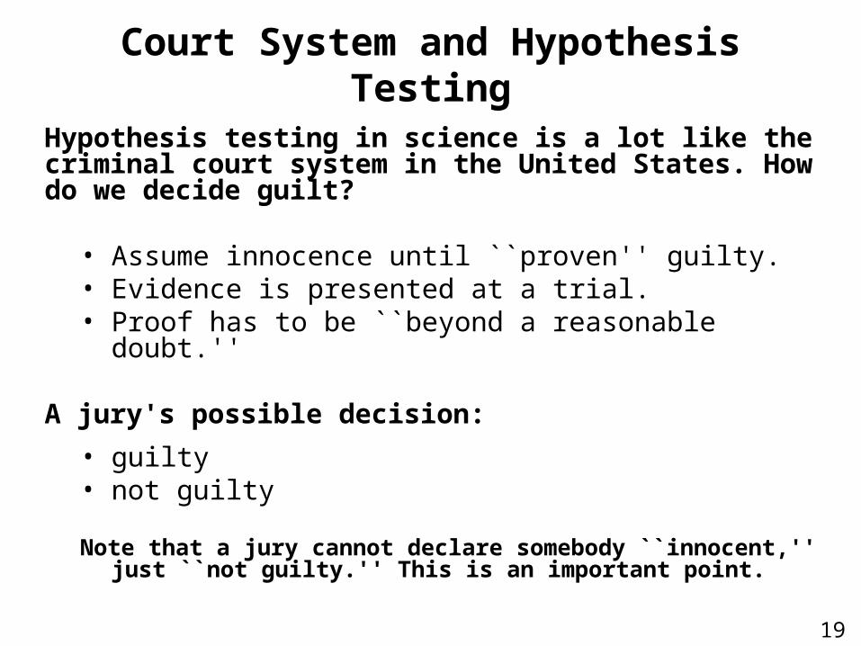
Court System and Hypothesis Testing
Hypothesis testing in science is a lot like the criminal court system in the United States. How do we decide guilt?
• Assume innocence until ``proven'' guilty. • Evidence is presented at a trial. • Proof has to be ``beyond a reasonable doubt.''
A jury's possible decision:
• guilty • not guilty
Note that a jury cannot declare somebody ``innocent,'' just ``not guilty.'' This is an important point.
20
nnxxnnxx2
22
1
21
2/2
_
1
_
21
2
22
1
21
2/2
_
1
_
--
ZZ
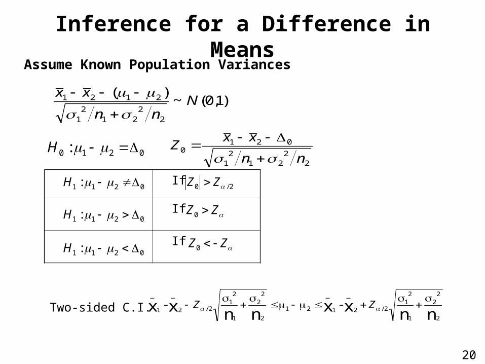
0210 : H
Inference for a Difference in Means
If
If
If
0211 : H
Assume Known Population Variances
)1,0(~)(
22
212
1
2121 Nnn
xx
22
212
1
0210
nn
xxZ
2/0 ZZ
0211 : H
0211 : H
ZZ 0
ZZ 0
Two-sided C.I.
21
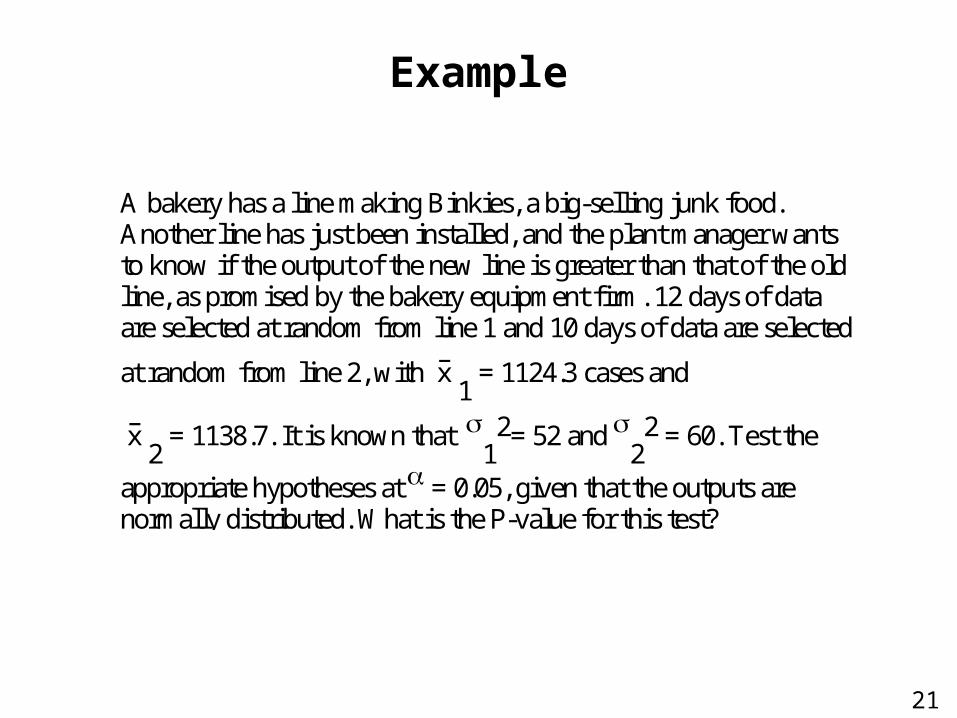
A bakery has a line making Binkies, a big-selling junk food. Another line has just been installed, and the plant manager wants to know if the output of the new line is greater than that of the old line, as promised by the bakery equipment firm. 12 days of data are selected at random from line 1 and 10 days of data are selected
at random from line 2, with x– 1 = 1124.3 cases and
x– 2 = 1138.7. It is known that
12= 52 and
22 = 60. Test the
appropriate hypotheses at = 0.05, given that the outputs are normally distributed. What is the P-value for this test?
Example
22
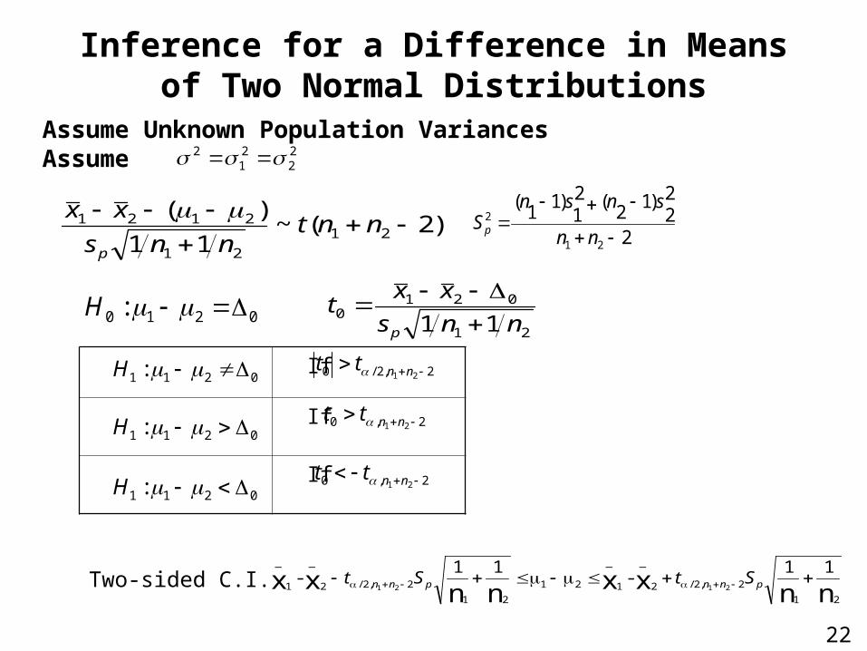
0210 : H
Inference for a Difference in Means of Two Normal Distributions
If
If
If
0211 : H
Assume Unknown Population VariancesAssume
)2(~11
)(21
21
2121
nnt
nns
xx
p
21
0210
11 nns
xxt
p
2,2/0 21 nntt
0211 : H
0211 : H
Two-sided C.I.
22
21
2
2,0 21 nntt
2,0 21 nntt
nnxxnnxx21
2,2/2
_
1
_
21
21
2,2/2
_
1
_ 11-
11-
2121 pnnpnn StSt
2
)12
( 22
)11
( 21
21
2
nn
snsnS p
23
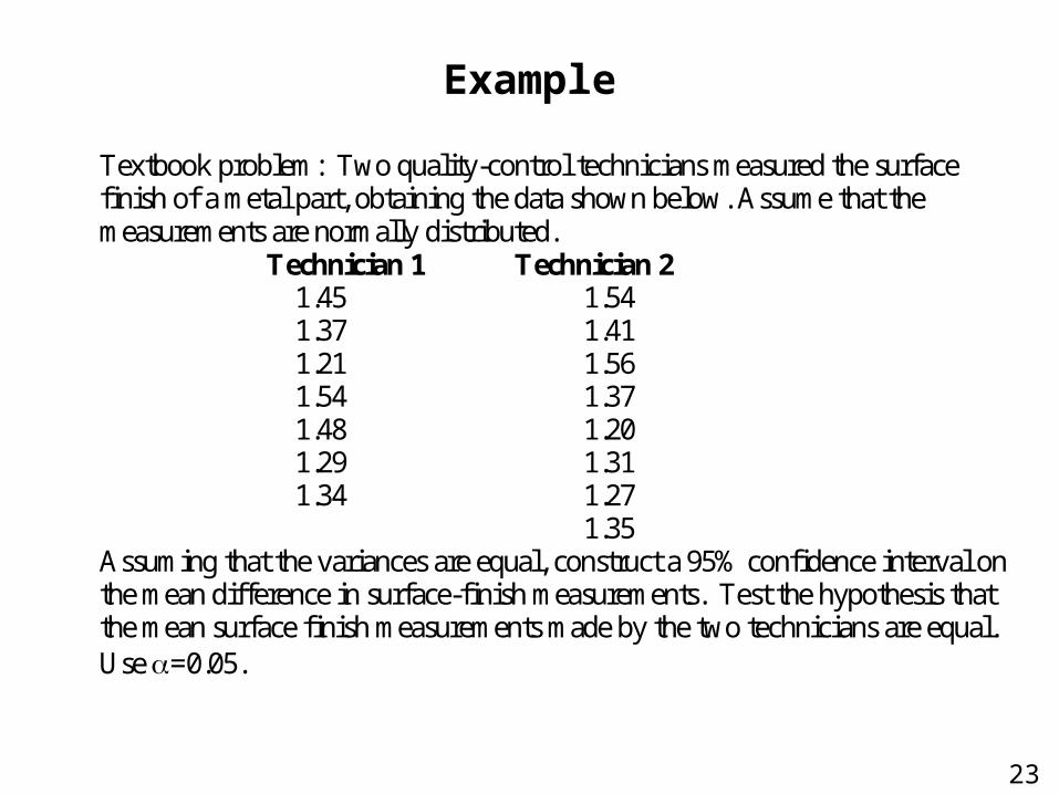
Textbook problem: Two quality-control technicians measured the surface finish of a metal part, obtaining the data shown below. Assume that the measurements are normally distributed. Technician 1 Technician 2
1.45 1.54 1.37 1.41 1.21 1.56 1.54 1.37 1.48 1.20 1.29 1.31 1.34 1.27
1.35 Assuming that the variances are equal, construct a 95% confidence interval on the mean difference in surface-finish measurements. Test the hypothesis that the mean surface finish measurements made by the two technicians are equal. Use =0.05.
Example
24
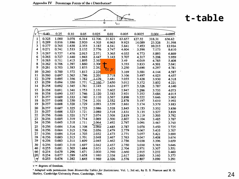
,t
t-table
25
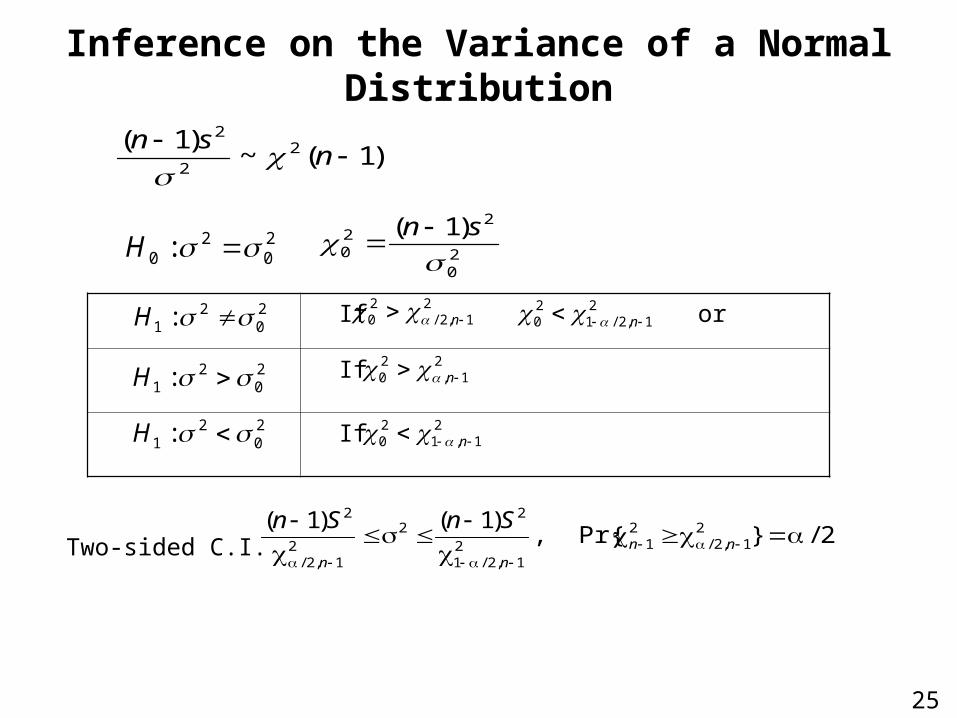
Inference on the Variance of a Normal Distribution
)1(~)1( 2
2
2
nsn
20
20 : H
If or
If
If
20
220
)1(
sn
21,2/
20 n2
02
1 : H2
1,2/120 n
20
21 : H
21,
20 n
20
21 : H 2
1,120 n
2/}Pr{,)1()1( 2
1,2/2
121,2/1
22
21,2/
2
nnnn
SnSnTwo-sided C.I.
26
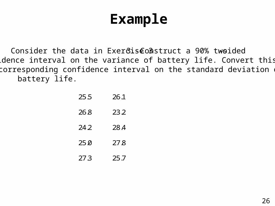
25.5 26.1 26.8 23.2 24.2 28.4 25.0 27.8 27.3 25.7
Example
Consider the data in Exercise 3 - 3. Construct a 90% two - sided confidence interval on the variance of battery life. Convert this into a corresponding confidence interval on the standard deviation of battery life.
27
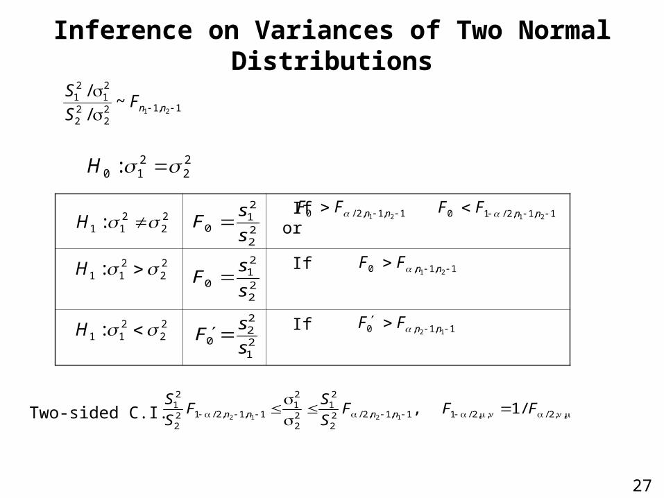
,,2/,,2/11,1,2/22
21
22
21
1,1,2/122
21 /1,
1212FFF
S
SF
S
Snnnn
Inference on Variances of Two Normal Distributions
1,122
22
21
21
21~
/
/
nnF
S
S
22
21
0 s
sF
22
210 : H
If or
If
If
1,1,2/0 21 nnFF 22
211 : H
1,1,2/10 21 nnFF
1,1,0 12 nnFF
22
211 : H
22
211 : H
1,1,0 21 nnFF
22
21
0 s
sF
21
22
0 s
sF
Two-sided C.I.
28
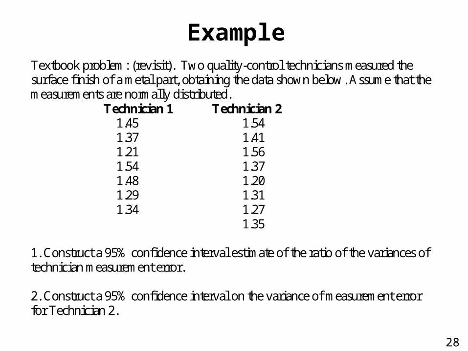
ExampleTextbook problem: (revisit). Two quality-control technicians measured the surface finish of a metal part, obtaining the data shown below. Assume that the measurements are normally distributed. Technician 1 Technician 2
1.45 1.54 1.37 1.41 1.21 1.56 1.54 1.37 1.48 1.20 1.29 1.31 1.34 1.27
1.35 1. Construct a 95% confidence interval estimate of the ratio of the variances of technician measurement error. 2. Construct a 95% confidence interval on the variance of measurement error for Technician 2.
29
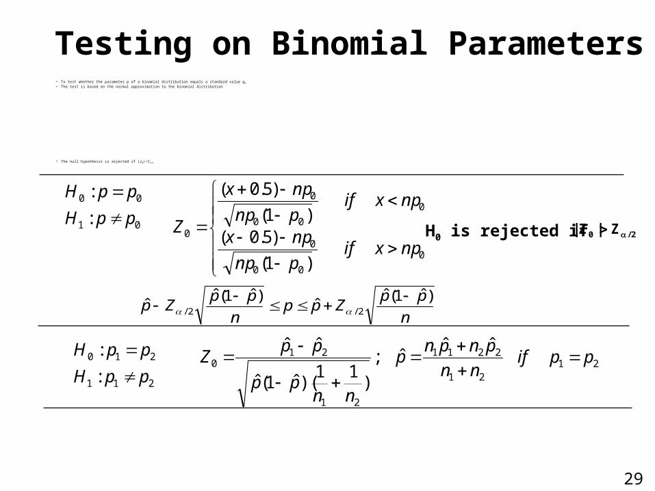
Testing on Binomial Parameters • To test whether the parameter p of a binomial distribution equals a standard value p0 • The test is based on the normal approximation to the binomial distribution
• The null hypothesis is rejected if |z0|>Z/2
01
00
:
:
ppH
ppH
0
00
0
0
00
0
0
)1(
)5.0()1(
)5.0(
npxifpnp
npx
npxifpnp
npx
Z
211
210
:
:
ppH
ppH
21
2211
21
210
ˆˆˆ;
)11
)(ˆ1(ˆ
ˆˆ
nn
pnpnp
nnpp
ppZ
21 ppif
2/0 Z|Z| H0 is rejected if
n
ppZpp
n
ppZp
)ˆ1(ˆˆ
)ˆ1(ˆˆ 2/2/
30
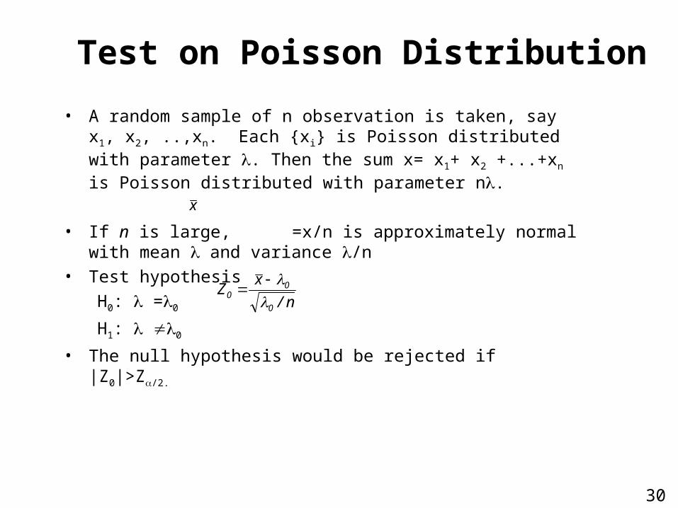
Test on Poisson Distribution
• A random sample of n observation is taken, say x1, x2, ..,xn. Each {xi} is Poisson distributed with parameter . Then the sum x= x1+ x2 +...+xn is Poisson distributed with parameter n.
• If n is large, =x/n is approximately normal with mean and variance /n
• Test hypothesis
H0: =0
H1: 0
• The null hypothesis would be rejected if |Z0|>Z/2.
n/
xZ
0
00
x
31
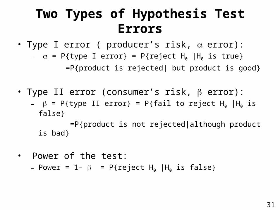
Two Types of Hypothesis Test Errors
• Type I error ( producer’s risk, error):– = P{type I error} = P{reject H0 |H0 is true}
=P{product is rejected| but product is good}
• Type II error (consumer’s risk, error):– = P{type II error} = P{fail to reject H0 |H0 is false}
=P{product is not rejected|although product is bad}
• Power of the test:– Power = 1- = P{reject H0 |H0 is false}
32
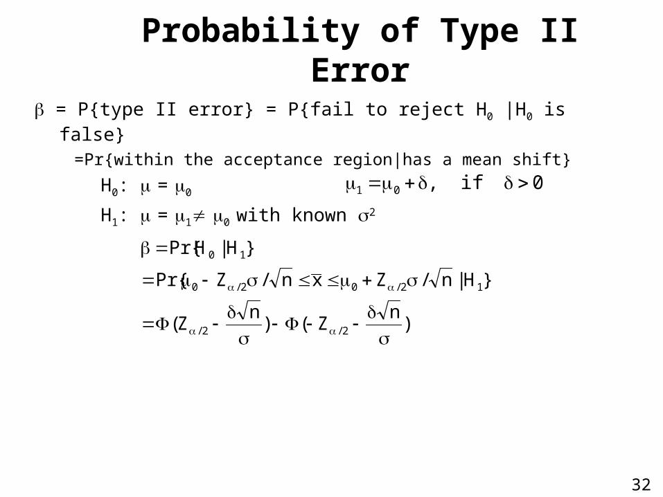
Probability of Type II Error
= P{type II error} = P{fail to reject H0 |H0 is false}
=Pr{within the acceptance region|has a mean shift}
H0: = 0
H1: = 1 0 with known 2 0if,01
)n
Z()n
Z(
}H|n/Zxn/ZPr{
}H|HPr{
2/2/
12/02/0
10
33
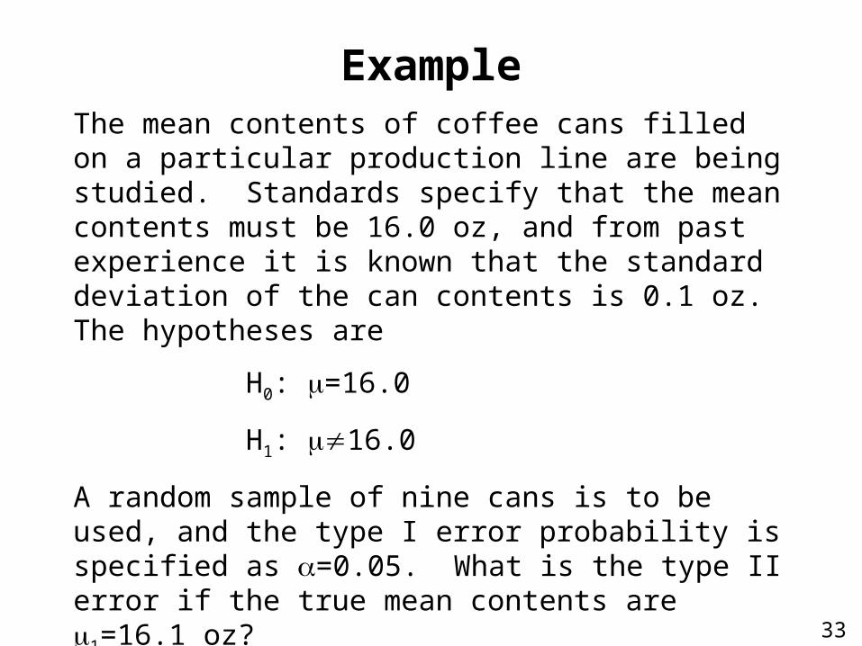
ExampleThe mean contents of coffee cans filled on a particular production line are being studied. Standards specify that the mean contents must be 16.0 oz, and from past experience it is known that the standard deviation of the can contents is 0.1 oz. The hypotheses are
H0: =16.0
H1: 16.0
A random sample of nine cans is to be used, and the type I error probability is specified as =0.05. What is the type II error if the true mean contents are 1=16.1 oz?
34
Properties of Type I & Type II Errors
Both types of errors can be reduced by increasing the sample size at the price of increased inspection costs.
For a given sample size, one risk can only be reduced at the expense of increasing the other risk.
35
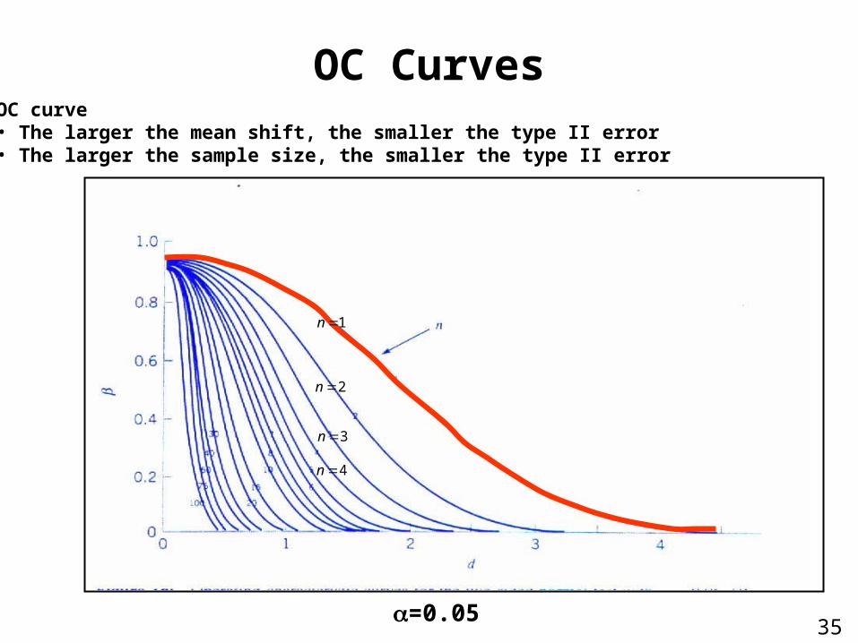
OC CurvesOC curve• The larger the mean shift, the smaller the type II error• The larger the sample size, the smaller the type II error
=0.05
1n
2n
3n
4n
36
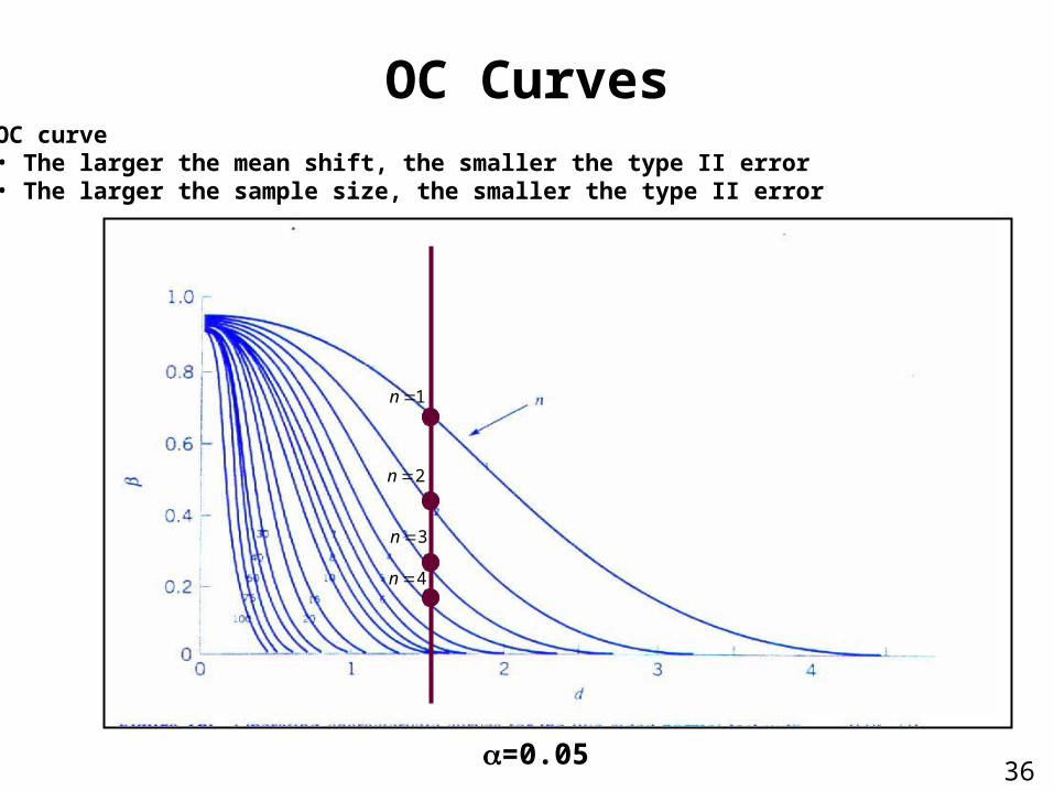
OC CurvesOC curve• The larger the mean shift, the smaller the type II error• The larger the sample size, the smaller the type II error
=0.05
1n
2n
3n
4n
37
Example
Suppose we wish to test the hypotheses
H0: =15
H1: 15
where we know that 2=9.0. If the true mean is really 20, what sample size must be used to ensure that the probability of type II error is no greater than 0.10? Assume that =0.05.
38
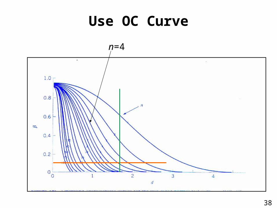
Use OC Curve
n=4