Advanced Predictive Guidance Navigation for Mobile …s2is.org/Issues/v1/n4/papers/paper3.pdf · · 2016-03-02Advanced Predictive Guidance Navigation for Mobile Robots: ... Advanced

Advanced Predictive Guidance Navigation for Mobile Robots:

A Novel Strategy for Rendezvous in Dynamic Settings

Faraz Kunwar and Beno Benhabib

Computer Integrated Manufacturing Laboratory Department of Mechanical and Industrial Engineering, University of Toronto

5 King’s College Road, Toronto, Ontario, Canada, M5S 3G8 email: [email protected]

Abstract—This paper presents a novel on-line trajectory planning method for the autonomous

robotic interception of moving targets in the presence of dynamic obstacles, i.e., position and

velocity matching (also referred to as rendezvous). The novelty of the proposed time-optimal

interception method is that it directly considers the dynamics of the obstacles as well as the target

in its interception maneuver: the velocities and accelerations of the obstacles and the target are

predicted in real-time for potential collisions. The method is designed to deal with highly-

maneuvering obstacles and targets. The interception maneuver is computed using an Advanced

Predictive Guidance Law.

Extensive simulation and experimental analyses, some of which are reported in this paper,

have clearly demonstrated the time efficiency of the proposed rendezvous method.

Index Terms— Target interception, on-line trajectory planning, rendezvous guidance.

INTERNATIONAL JOURNAL ON SMART SENSING AND INTELLIGENT SYSTEMS, VOL. 1, NO. 4, DECEMBER 2008INTERNATIONAL JOURNAL ON SMART SENSING AND INTELLIGENT SYSTEMS, VOL. 1, NO. 4, DECEMBER 2008INTERNATIONAL JOURNAL ON SMART SENSING AND INTELLIGENT SYSTEMS, VOL. 1, NO. 4, DECEMBER 2008

858

mailto:[email protected]

I. INTRODUCTION

Real world mobile robotic environments have, typically, time-varying topologies, with numerous

objects moving with respect to each other. Furthermore, such environments are subject to

uncertainties as complete information and future trajectories of objects cannot be assumed to be

known a priori. Thus, there rises a need for autonomous routing decisions – on-line motion

planning and execution of robotic vehicle trajectories. A preferred solution to this problem would

be one that takes into consideration the kinematic constraints of the vehicle, explicitly copes with

dynamically moving objects, and is analytical. Furthermore, high-level autonomy and time

optimality would be desirable during motion planning via real-time sensory-data collection about

the objects. In this context, the focus of this paper is the development of a generic guidance-

based methodology that would provide an autonomous robotic vehicle with the capability to

time-optimally rendezvous with a moving target (matching position and velocity) in the presence

of mobile obstacles.

The problem of robotic-vehicle interception in obstacle-cluttered environments using a

Rendezvous-Guidance (RG) method augmented with a Modified Exact Cell Decomposition

method for rendezvous was first addressed in [1]. The time optimality of this method was further

improved in [2] through the use of a Velocity Obstacle (VO) approach. The modified method,

however, still only ensured near-optimal performance for rendezvous with non-maneuvering

targets. Therefore, herein, a new guidance law that can yield optimal rendezvous with targets

having high degree of maneuverability is proposed: This novel guidance law utilizes an

Extended Kalman Filter (EKF) to estimate the target’s state, as well as directly makes use of the

dynamic characteristics of the obstacles to estimate their future states. These estimates are used

to predict potential collisions between the pursuer and the obstacles by using the Collision Cone

(CC) method. A brief overview of the pertinent literature is provided below.

A. Guidance-Based Interception

Missile-guidance techniques have been classified into five main categories: Line-Of-Sight (LOS)

guidance; Pure Pursuit (PP); Proportional Navigation Guidance (PNG); Optimal Guidance (OG);

and, other guidance methods including the use of differential game theory [3, 4]. Missile-

guidance laws assume that the future trajectory of the target is completely defined either

analytically or by a probabilistic model [5-7]. However, the problem of velocity matching, as

Faraz Kunwar and Beno Benhabib, Advanced Predictive Guidance Navigation for Mobile Robots:A Novel Strategy for Rendezvous in Dynamic Settings

859

dealt in this paper, is not typically addressed in missile-guidance applications.

The PNG law uses the homing triangle for computing the acceleration of an interceptor

pursuing an evading target. The homing triangle is defined by the pursuer, the target, and the

point of interception. This control law makes the pursuer’s acceleration normal to its path and

proportional to the rate of change of the LOS vector to the target. Due to its low computational

requirements, simplicity of on-board implementation, and time optimality characteristics, PNG

has been the most widely used guidance technique [8]. The need for velocity matching has

resulted in a new class of guidance methods, commonly referred to as Rendezvous-Guidance

(RG) methods. A PNG-based RG method for the docking problem of two space vehicles was

proposed in [9]. In [10], the use of exponential-type guidance was suggested for asteroid

rendezvous. The problem of rendezvous with an object capable of performing evasive maneuvers

in order to avoid rendezvous was addressed in [11].

The utilization of a guidance-based technique in robot-motion planning, with the purpose of

improving upon the interception time achievable by visual-servoing techniques, was first

reported in [12-14]. Although, these works showed that guidance-based methods could yield

shorter interception times compared to other available techniques, all were limited to

environments with no obstacles. Further work carried out in our laboratory augmented guidance-

based methods with the capability to avoid mobile obstacles [1-2, 15]. These are based on the PN

technique, which basically deals with first-order derivatives of target/obstacle velocity, though,

they are not very effective in the presence of highly maneuvering target/obstacles.

In present day applications, the maneuverability of the target as well as the obstacles is

increasingly becoming more complex. Especially in cases that involve human-machine

interactions, for example, in public places like museums, hospitals, or factory floors. Such

applications necessitate better tracking of the obstacles as well as of the target than is achievable

by models based on PN techniques. The reason for the inadequate tracking performance of such

models is that the higher-order derivatives in the case of very highly maneuvering targets are

significant. Therefore, in this paper, we present a novel method that can deal with highly-

maneuvering targets by inherently considering the higher-order terms of the target/obstacle

model.


860

B. Obstacle Avoidance

Motion-planning problems for mobile robots have been classified as static or dynamic. For the

former, the obstacle information is assumed to be known to the planner in its entirety prior to

planning. For the latter, information about the environment becomes known to the planner only

during run-time and often during the execution of a partially-constructed plan.

Static motion-planning approaches, such as potential field and vector field histogram,

calculate the desired motion direction and steering commands in two separate steps [16-18]. In

the first step, the obstacle-avoidance method provides intermediate destination points that

connect a collision-free path from the robot to the target. In the second step, acceleration

commands are derived for the path generated for the motion of the robot. Such a methodology

would not be acceptable for a dynamic environment with fast moving obstacles, where the

uncertainty about the environment prevents the computation of a solution that is guaranteed to

succeed. Furthermore, static obstacle-avoidance methods have been developed to deal with

geometric constraints, more specifically, holonomic systems. For non-holonomic systems such as

mobile robots, kinematic constraints make time derivatives of some configuration variables non-

integrable and, hence, a collision-free path in the configuration space is not necessarily feasible

(i.e., it may not be achievable by steering controls) [19-20].

In dynamic obstacle avoidance methods, information about the environment becomes known

to the planner only during runtime and often during the execution of a partially constructed plan.

The Curvature-Velocity (CV) [21] and the Dynamic Window (DW) [22] methods are based on

the steer-angle-field approach [23]. The CV method chooses a location in translational and

rotational velocity space which satisfies constraints placed on the robot and maximizes an

objective function [24]. The Lane Curvature Method [25] improves upon the CV method by

using a directional-lane method. The DW method considers the kinematic and dynamic

constraints of a mobile robot [26]. Kinematic constraints are taken into account by directly

searching the velocity space of the robot. The search space is reduced to a dynamic window

representing the velocities achievable by the robot in a given interval of time. In spite of the good

results for obstacle avoidance at high velocities achieved by both CV and DW methods, local-

minima problem persists. In order to overcome this shortcoming, the DW Method was integrated

with a gross-motion planner in [27] and extended to use a map in conjunction with sensory

information in [28] to generate collision-free motions.


861

The above approaches require a priori information about the environment. The Velocity

Obstacle (VO) approach proposed in [29], on the other hand, determines potential collisions and

computes collision-free paths for robots moving in dynamic environments. The VO method was

extended in [30] to include objects moving along non-linear trajectories.

The work presented in this paper uses concepts that are rooted in missile guidance/aerospace

literature for obstacle avoidance so that the method provides an elegant integration with the

navigation algorithm used for interception. Our objective is, thus, developing a novel obstacle-

avoidance navigation law based on proven navigation-guidance principles.

Up to now, most of the existing methods have dealt with obstacle avoidance by non-

holonomic systems in one of two ways. The first is to exclusively focus upon motion planning

under non-holonomic constraints without considering obstacles – differential geometry [31],

differential flatness [32], input parameterization [33-35], and optimal control [36]. In particular,

the non-holonomic motion-planning problem is recast as an optimal control problem, where

Pontryagin’s Maximum Principle is applied. As first shown in [37] and later improved in [38],

the feasible shortest path for a point robot under two boundary conditions is a concatenation of

simple pieces (such as an arc and a straight line segment) that belong to three-parameter families

of controls.

The second way in dealing with obstacle avoidance by non-holonomic systems is to modify

the resultant solution from a holonomic planner so that the resulting path is feasible. For

example, the online sub-optimal obstacle avoidance algorithm in [39] is based on the Hamilton–

Jacobi–Bellman equation ([40], [41]), deals only with stationary obstacles, and the planned path

is holonomic, whose feasibility has to be verified in case of a non-holonomic mobile robot.

Similarly, the non-holonomic path planner in [42] generates a path by ignoring non-holonomic

constraints and it is, then, made feasible via approximation by using a sequence of optimal path

segments such as those in [43].

In this paper, we consider the non-holonomic constraints of the pursuer directly within the

navigation algorithm. It is ensured that all acceleration commands generated by the

navigation/obstacle-avoidance algorithm are within the acceleration capabilities of the pursuer

and can be executed at the next time instant. Although the algorithm presented in this paper is

primarily designed for vehicular robots yet it can also be applied to humanoid robots, e.g., the


862

control system for a biped presented in [44] can easily be integrated with the proposed algorithm

to enable the robot to avoid static and dynamic obstacles while moving in the desired direction.

II. PROPOSED SYSTEM

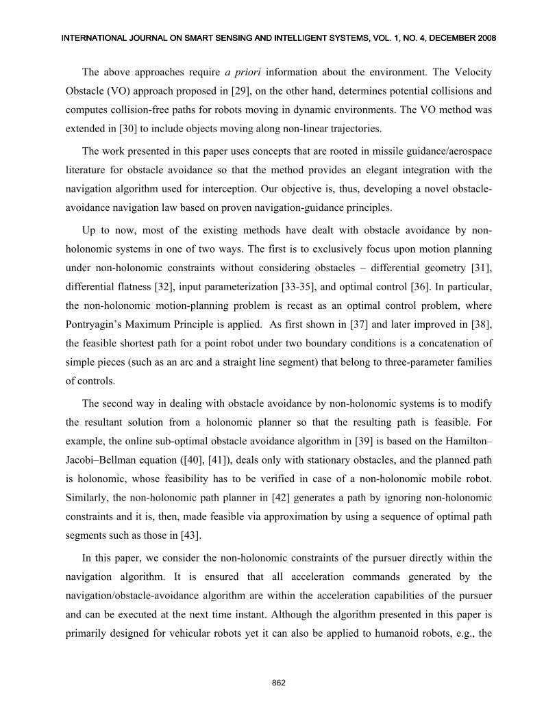
A schematic diagram of the proposed rendezvous system is shown in Figure 1: First, the states of

the pursuer, obstacles, and target are estimated and sent to the path planner; The path planner,

then, generates a single acceleration command for the pursuer, for time-optimal rendezvous

while avoiding obstacles (as detailed in Section III) – if obstacle avoidance is not needed, the

pursuer obtains its acceleration command directly from the navigation algorithm.

In the following sub-sections, first the methodology for obtaining a model of the pursuer is

detailed and, subsequently, the proposed novel guidance and obstacle-avoidance methods are

presented.

Figure 1: Proposed Rendezvous System.


863

A. The Kinematic Model of the Mobile Robot

The kinematic model for a differentially-driven wheeled mobile robot (as the ones used in our

experiments) is selected as the basis for this work:

[ ][ ]

cos 0sin 0 ,

0 1

Tcc c

c T

xy x y

yu

λλ

λλ

⎡ ⎤ ⎡ ⎤=⎡ ⎤⎢ ⎥ ⎢ ⎥= ⎢ ⎥⎢ ⎥ ⎢ ⎥ =⎣ ⎦⎢ ⎥ ⎢ ⎥⎣ ⎦ ⎣ ⎦

&

&&

v

vω ω , (1)

where y is the system state; the robot is located at (xc, yc) turning to the right; λ is the robot

heading angle with respect to the X-axis; and, the control u consists of the linear velocity

v and the angular velocity ω. Although in (1) the controls of the mobile robot are its

linear and angular velocities, the actual commands provided to the vehicle are the right

and left wheel velocities, Figure 2.

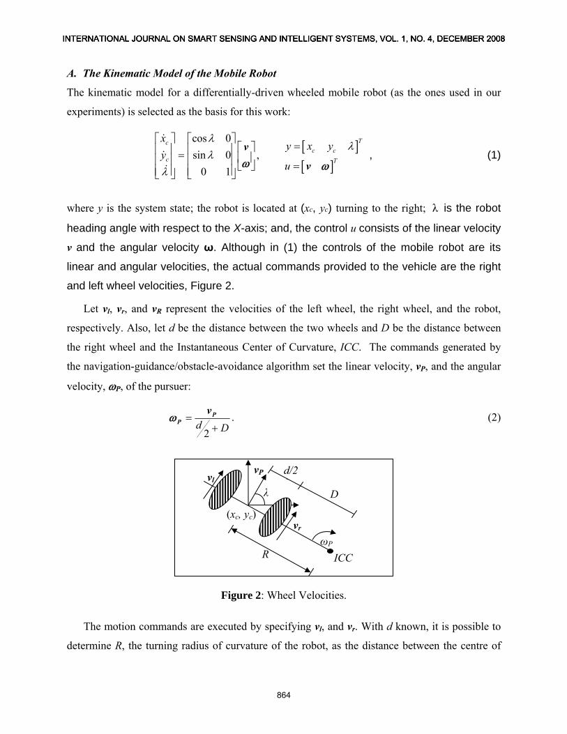
Let vl, vr, and vR represent the velocities of the left wheel, the right wheel, and the robot,

respectively. Also, let d be the distance between the two wheels and D be the distance between

the right wheel and the Instantaneous Center of Curvature, ICC. The commands generated by

the navigation-guidance/obstacle-avoidance algorithm set the linear velocity, vP, and the angular

velocity, ωP, of the pursuer:

2d D

=+P

Pv

ω . (2)

R ωP

d/22

D

vP

vr

vl

ICC

(xc, yc)

λ

Figure 2: Wheel Velocities.

The motion commands are executed by specifying vl, and vr. With d known, it is possible to

determine R, the turning radius of curvature of the robot, as the distance between the centre of


864

the robot and ICC. The wheel velocities are determined using the kinematics Equations (3) to

(5) given below,

2+

= l rP

v vv , (3)

dDD += lr vv

, and (4)

whr=l lv ω , whr=rv rω , (5)

where rwh is the radius of the wheel, and ωl and ωr are the angular velocities of the left and right

wheel, respectively.

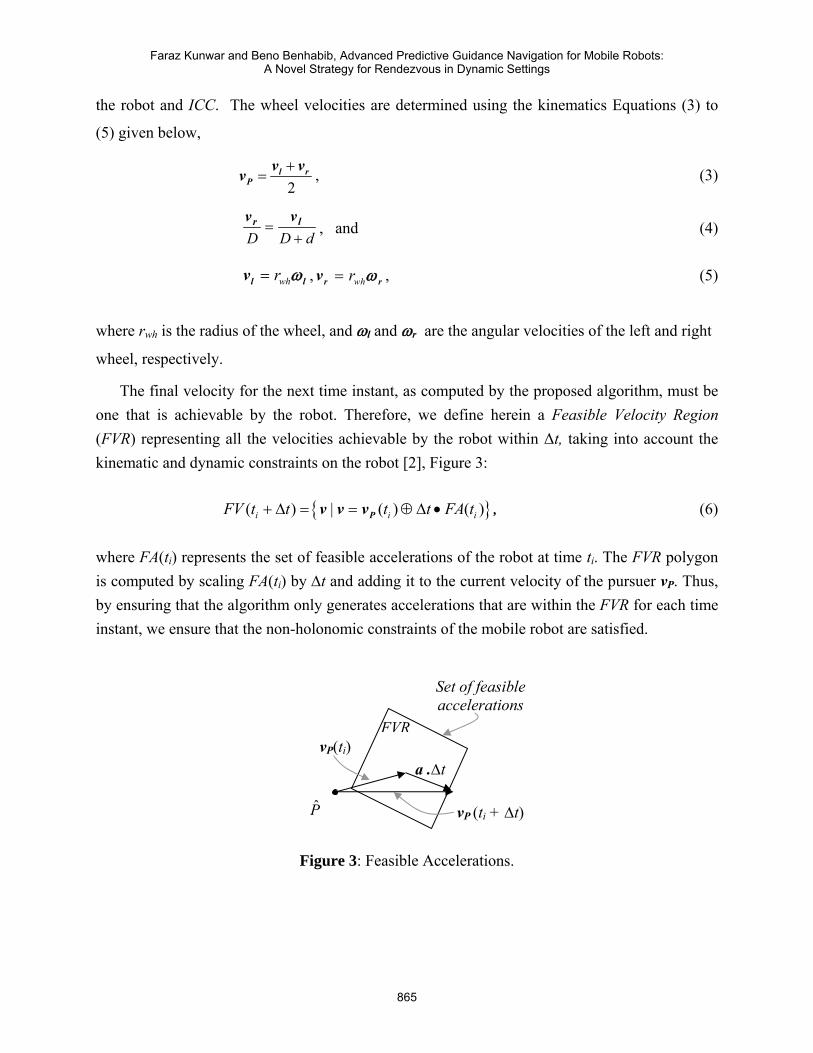
The final velocity for the next time instant, as computed by the proposed algorithm, must be one that is achievable by the robot. Therefore, we define herein a Feasible Velocity Region (FVR) representing all the velocities achievable by the robot within Δt, taking into account the kinematic and dynamic constraints on the robot [2], Figure 3:

{ }( ) | ( ) (i iFV t t t t FA t+ Δ = = ⊕ Δ •Pv v v )i , (6)

where FA(ti) represents the set of feasible accelerations of the robot at time ti. The FVR polygon is computed by scaling FA(ti) by Δt and adding it to the current velocity of the pursuer vP. Thus, by ensuring that the algorithm only generates accelerations that are within the FVR for each time instant, we ensure that the non-holonomic constraints of the mobile robot are satisfied.

Set of feasible accelerations

vP(ti) FVR

P̂ vP (ti + Δt)

a .Δt

Figure 3: Feasible Accelerations.


865

B. Interception Using the Advanced Predictive Guidance Law

This section describes the new Advanced Predictive Guidance Law (APGL) based target-

interception method proposed in this paper. The Proportional Navigation Law (PNL) is reviewed

first to provide the mathematical basis for the APGL.

Theoretically, the PNL issues commands perpendicular to the instantaneous pursuer-target

line-of-sight, which are proportional to the line of sight rate and closing velocity:

PNL

N λ=cn cv , (7)

where nc is the acceleration command, N is a unit-less gain (usually in the range of 3-5) known

as the effective navigation ratio [3], vc is the pursuer-target closing velocity, and λ is the LOS

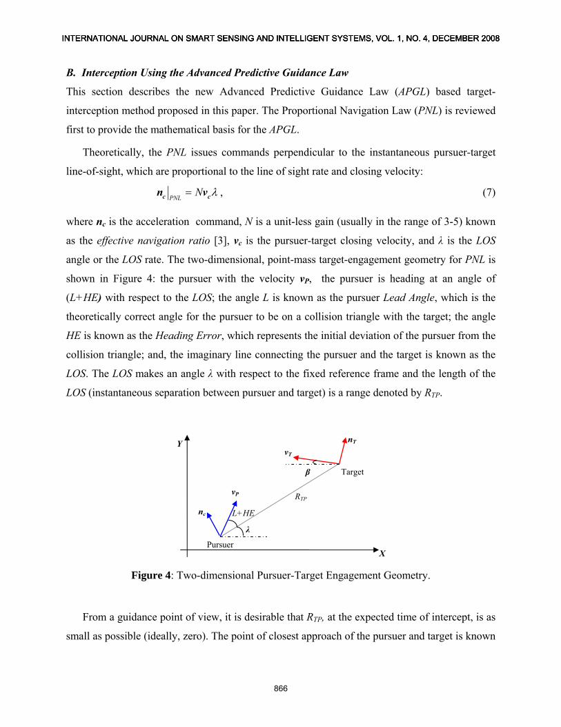
angle or the LOS rate. The two-dimensional, point-mass target-engagement geometry for PNL is

shown in Figure 4: the pursuer with the velocity vP, the pursuer is heading at an angle of

(L+HE) with respect to the LOS; the angle L is known as the pursuer Lead Angle, which is the

theoretically correct angle for the pursuer to be on a collision triangle with the target; the angle

HE is known as the Heading Error, which represents the initial deviation of the pursuer from the

collision triangle; and, the imaginary line connecting the pursuer and the target is known as the

LOS. The LOS makes an angle λ with respect to the fixed reference frame and the length of the

LOS (instantaneous separation between pursuer and target) is a range denoted by RTP.

Pursuer

Target

X

Y

RTP

nT

vT

vP

nc

β

λ

L+HE

Figure 4: Two-dimensional Pursuer-Target Engagement Geometry.

From a guidance point of view, it is desirable that RTP, at the expected time of intercept, is as

small as possible (ideally, zero). The point of closest approach of the pursuer and target is known


866

as the miss distance. The closing velocity, vc, is defined as the negative rate of change of the

distance from the pursuer to the target:

TPR= − &

cv . (8)

Therefore, at the end of the interception, when the pursuer and the target are in closest proximity,

the sign of vc would change. The desired acceleration command nc is perpendicular to the

instantaneous line of sight.

As shown in Figure 4, the target can maneuver evasively with an acceleration nT. The

angular velocity of the target is, thus, expressed as:

β =& T

T

nv

, (9)

where vT is the is the magnitude of the target velocity. Since the acceleration command is

perpendicular to the instantaneous LOS, the pursuer acceleration command in the fixed reference

frame has the following components:

sincos

PNL

PNL

λλ

= −=

Px c

Py c

a na n

.、 (

、10、、

)、

A pursuer employing PNL does not move directly toward the target, but, in a direction to

lead the target. The theoretical pursuer Lead angle, L, can be found by application of the law of

sines, yielding:

1 sin( )

sinLβ λ− +

= T

P

vv

. (11)

The LOS angle is, then, expressed in terms of the relative separation components:

1tan TPyR

λ −=TPxv

. (12)

The LOS rate is expressed:


867

2TPx TPy

TP

R RR

λ−

=& TPy TPxv v (13)

Any initial angular deviation of the pursuer from the collision triangle is defined by the angle

HE. The initial pursuer velocity components are, therefore, expressed in terms of the theoretical

lead angle, L, and actual heading error, HE, as

(0) cos( )(0) sin( )

L HEL HE

λλ

= += + +

Px P

Py P

v vv v

+.、 (

、14、、

)、

Let us define a Zero-Effort Miss (ZEM, the bracketed term in Equation (15) below) as a

prediction of by how much the pursuer would miss the target, if the target were to continue as it

has done in the past and the pursuer was issued no further acceleration commands (i.e., zero

effort). As shown in [3], PNL can also be considered as a guidance law in which the acceleration

command is proportional to the ZEM and inversely proportional to the square of the time

remaining to intercept:

2 [ ]goPNLgo

N y ytt

′= + &cn , (15)

where y is the relative distance between the pursuer and the target, is the relative target rate and

t

y&

go is the time to go before the intercept occurs ( go TPt R= cv ). Thus, for PNL, ZEM assumes that

the target is not maneuvering. This does not imply that the PNL cannot intercept maneuvering

targets, but rather that it is not optimal in their interception.

Advanced Predictive Guidance Law

In order to overcome the limitations of PNL, an Advanced Predictive Guidance Law, APGL, is

proposed in this paper to improve the performance of a pursuer for fast-maneuvering targets. In

this guidance law, the predicted intercept with the target is calculated on-line by integrating the

non-linear pursuer and target equations forward in time at each guidance update. This proposed

law overcomes the limitations of PN to improve the performance of an interceptor especially

against a maneuvering target. As with PN, the APG tries to yield zero miss distance while

minimizing the following:


868

2

0

( ) 0 subject to minimizing ( ) .Ft

Fy t t dt= ∫ ac (16)

The proposed APG law can be expressed in state-space form as

2

0 1 0 0 00 0 1 0 1

,0 0 0 1 00 0 0 0

T T

T T

y yy yy yy y

F G

ω

⎡ ⎤ ⎡ ⎤⎡ ⎤ ⎡⎢ ⎥ ⎢ ⎥⎢ ⎥ ⎢−⎢ ⎥ ⎢ ⎥⎢ ⎥ ⎢= +⎢ ⎥ ⎢ ⎥⎢ ⎥ ⎢⎢ ⎥ ⎢ ⎥⎢ ⎥ ⎢−⎣ ⎦ ⎣⎣ ⎦ ⎣ ⎦

&

&& &

&&& &&

&&&& &&&

ca

⎤⎥⎥⎥⎥⎦

(17)

where ω is the target maneuver frequency, y is the relative position between the pursuer and the

target, is the relative velocity between the pursuer and the target, &y &&Ty is the target acceleration

and &&&Ty is the target jerk. The final state of the system at any time can also be expressed as

( ) ( - ) ( ) ( - ) ( ) ( ) ( ),Ft

F F Ft

x t t t x t t G u dΦ Φ λ λ λ= + ∫ λ (18)

where ( )x t is the system state vector and ( )tΦ is the fundamental matrix and is related to F

according to

1( ) ( ) .t L sI FΦ − ⎡= −⎣1− ⎤⎦ (19)

Solving (19) yields

( ) ( )

( )2 3

2

1 cos 1 cos1

1 cossin0 1( ) ,sin0 0 cos

0 0 sin cos

t tt

ttt

tt

t t

ω ωω ω

ωωΦ ω ω

ωωω

ω ω ω

⎡ ⎤− −⎢ ⎥⎢ ⎥⎢ ⎥−⎢= ⎢⎢ ⎥⎢ ⎥⎢ ⎥

−⎢ ⎥⎣ ⎦

⎥⎥ (20)

Substituting and G matrices into (18) and simplifying yields the proposed APGL for

maneuvering targets which is expressed as

Φ

2 2 2 3

1 cos sin3 33 .go go goAPG

go go

t t tt t

ω ω ωω ω

− −⎡ ⎤ ⎡= + +⎢ ⎥ ⎢

⎣ ⎦ ⎣& && &&&c c Ta v yλ

⎤⎥⎦

Ty (21)


869

The above Equation (21) shows that in essence the APG is similar to the PN and APN

wherein, the guidance commands are still proportional to the ZEM and inversely proportional to

the square of tgo. However, the new guidance law consists of three terms: one proportional to the

LOS rate, another proportional to the target acceleration, and a third proportional to the target

jerk.

In order to better understand the relationship between the new guidance law and its

predecessors, let us consider the case in which the target is not maneuvering, i.e., the target

maneuvering frequency is zero. By using Taylor series approximation, the APG law is simplified

to:

2 3

20

3lim .2 6go go

goAPGgo

t ty yt

tω→

⎡ ⎤= + + +⎢

⎢ ⎥⎣ ⎦&& &&&ca y ⎥T Ty (22)

The above is simply an Augmented Proportional Navigation Law (APNL) with an effective

navigation ratio of 3 plus an extra term to account for target jerk, which implies that APGL

requires, in addition to the LOS rate, an estimate of the target maneuver frequency, target jerk,

and tgo. These terms can be estimated in a number of ways for example, by using external sensors

or by implementing an Extended Kalman Filter (EKF). In this thesis, a five-state EKF is used to

predict target characteristics. Details on how to implement a suitable EKF for this problem are

given in [7]. A general method for the development of an EKF is given in Appendix A.

Thus, after the estimation all the information necessary to calculateAPGca , using (21), is

now available. The acceleration for the next time instant using APGL is, finally, obtained by

using the value obtained from (21) in (10).

sin , and

cos .APG

APG

λ

λ

= −

=APGx c

APGy c

a a

a a (23)

Generating the Rendezvous Command

If the pursuer were to follow the acceleration commands generated in (23), it would intercept the

target at an optimal time in the future. However, in order to rendezvous with the target, the

velocity of the pursuer must also match the velocity of the maneuvering target at the time of

interception.


870

Let us assume that the deceleration capability of the robot in the direction of motion is given

by A. This acceleration would be used to bring the closing velocity down to zero. In deciding on

the rendezvous maneuver, there are two primary issues that need to be resolved: First, the

magnitude of the maximum closing velocity needs to be determined and, second, the time instant

to switch between target-interception and target-rendezvous strategies needs to be carefully

chosen (the former would lead to a collision with the target).

Let us denote as the magnitude of the maximum allowable closing/rendezvous velocity

(hence, the superscript rend),

&rendmaxr

got as the time remaining to intercept the target from the current

instant, and RTP as the relative distance between the pursuer and the target. In order to

simultaneously reduce the relative velocity and the relative distance to zero, the following

expressions need to be implemented:

( )

0go

go

t t

t

= −

− =

&

&

rendmax

rendmax

v r A

r A, and (24)

0

2

( ) ( )

1 02

Ft

TP

TP go go

r t R d

R t t

τ τ= −

− −

∫&rendmax

v

r A =. (25)

The maximum instantaneous allowable closing velocity is obtained by solving (24) and (25):

Arr rend

max 2=& . (26) The maximum closing velocity as imposed by the frequency of velocity command generation

by the trajectory planner for a fast asymptotic interception is given by:

Δn t=&crmax

rr . (27)

The value of above is determined experimentally. The final allowable closing velocity

component of the velocity command is, then, obtained by considering (26) and (27)

simultaneously:

n

cr max

rend max

rel max r,rv &&min= . (28)


871

The next algorithmic step is to determine the instant to switch between interception and

rendezvous strategies. This is obtained by finding the instant at which the velocity represented by

can be achieved by the pursuer within the sampling period Δt, namely, the instant at which

the velocity lies within the Feasible Velocity Region (FVR) as defined in (6).

relmaxv

relmaxv

C. Predictive Obstacle Avoidance

In this work, for the purpose of obstacle avoidance, we have used concepts that are rooted in the

missile-guidance/aerospace literature [44]. The motivation behind using such an approach stems

from the fact that collision avoidance and collision achievement are, in principle, two aspects of

the same problem. Since the proposed obstacle-avoidance method is based on the principles of

missile guidance, it allows for an elegant integration with the proposed navigation guidance law

used herein (i.e., APGL).

Majority of existing dynamic obstacle-avoidance algorithms (e.g., [25]-[30]) attempt to avoid

all obstacles which are in the vicinity of the vehicle by evaluating a time-based or distance-based

criterion. This may lead to a significant increase in computational complexity in evaluating

obstacles which are not on a direct collision course with the vehicle. Thus, the two important

decisions in our proposed algorithm are to decide (i) whether avoidance is necessary with an

obstacle and, if necessary, (ii) whether the APGL commanded acceleration is sufficient to avoid

it.

Obstacle-Avoidance Navigation Law (OANL)

The key objective to collision avoidance is to maintain a predefined safe distance between the

pursuer and the obstacle. Let us consider the collision-avoidance problem shown in Figure 5. The

pursuer is moving on a 2D plane in the presence of another mobile robot that is designated as an

obstacle.

Since for the purpose of the APGL, the pursuer is considered to be a point mass, the OANL

must be based on a similar principle. This is achieved by reducing the pursuer to a point mass

and increasing the size of the obstacle by the size of the pursuer. For simplicity, the obstacle is

approximated by a circle that envelops the obstacle. Therefore, when increasing the size of the

obstacle by the size of the pursuer, one simply increases the radius of the bounding circle of the

obstacle by the radius of the pursuer.


872

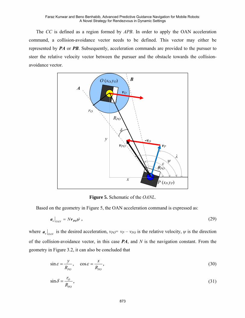
The CC is defined as a region formed by APB. In order to apply the OAN acceleration

command, a collision-avoidance vector needs to be defined. This vector may either be

represented by PA or PB. Subsequently, acceleration commands are provided to the pursuer to

steer the relative velocity vector between the pursuer and the obstacle towards the collision-

avoidance vector.

vO

vP

RPO

rO

ψ

vPO

A

P (xP,yP)

B O (xO,yO)

λ

θPO

x

y

ε

δ

-vO

Figure 5. Schematic of the OANL.

Based on the geometry in Figure 5, the OAN acceleration command is expressed as:

OANN ψ= &c Pa v O , (29)

where OANca is the desired acceleration, vPO= vP – vPO is the relative velocity, ψ is the direction

of the collision-avoidance vector, in this case PA, and N is the navigation constant. From the

geometry in Figure 3.2, it can also be concluded that

sin , cosPO PO

y xR R

ε ε= = , (30)

sin O

PO

rR

δ = , (31)


873

sinPO Py v Oθ= −& , and (32)

POψ θ= +&& ε& . (33)

Differentiatin Equations (31) and (32) with respect to time t and substituting into (33) yields,

(sintan tan

cosPO PO PO

PO PO

v RR R

θ )ψ ε δε

⎛ ⎞= − + +⎜

⎝ ⎠

&& ⎟ . (34)

The acceleration for the next time instant using OANL is obtained by substituting the above value

of OANca into an equation similar to (10):

sin

cos

λ

λ

= −

=OANx c OAN

OANy c OAN

a a

a a . (35)

Prediction of Obstacle Parameters

In this thesis, it is assumed that dynamic obstacles may have different types of motions.

Furthermore, as shown in the previous section, the OANL depends on an accurate interpretation

of the relative velocity between the pursuer and the obstacle. Therefore, in order to predict the

movements of highly maneuverable obstacles one needs to accurately track the obstacles. This

may be achieved by means of a KF that also considers higher order derivatives in the tracking

model for the obstacles. The higher order derivatives in the KF tracking model include obstacle

acceleration and jerk. This can be written in a state-space framework as

0 1 0 0 00 0 1 0 0

( )0 0 0 1 00 0 0 0 1

y yy yd w ty ydty y

⎡ ⎤ ⎡ ⎤ ⎡ ⎤ ⎡ ⎤⎢ ⎥ ⎢ ⎥ ⎢ ⎥ ⎢ ⎥⎢ ⎥ ⎢ ⎥ ⎢ ⎥ ⎢ ⎥= +⎢ ⎥ ⎢ ⎥ ⎢ ⎥ ⎢ ⎥⎢ ⎥ ⎢ ⎥ ⎢ ⎥ ⎢ ⎥⎣ ⎦ ⎣ ⎦ ⎣ ⎦ ⎣ ⎦

&

& &&

&& &&&

&&& &&&&

, (36)

where denote the position, velocity, acceleration, and jerk of the target,

respectively, and w(t) is the system noise. The measurement vector at the (k + 1)

, , , and y y y y& && &&&

th instant can be

expressed in the general form as shown in Equation (37) where v(t) is the measurement noise.

[ ]1 0 0 0 ( ).T

T

T

yy

y v tyy

⎡ ⎤⎢ ⎥⎢ ⎥=⎢ ⎥⎢ ⎥⎣ ⎦

&

&&

&&&

+ (37)


874

Since measurements are not taken continuously but, every, Ts, seconds, the system model

needs to be discretized. The fundamental matrix in discrete form is approximated by Equation

(38) which is basically a two term Taylor Series expansion:

2 3

2

1 20 1 20 0 10 0 0 1

K

T T TT T

Tϕ

⎡ ⎤⎢ ⎥⎢=⎢⎢ ⎥⎢ ⎥⎣ ⎦

6

⎥⎥ . (38)

The discrete order process noise matrix is obtained from the continuous process noise matrix

according to:

7 6 5 4

6 5 4 32

5 4 3 2

4 3 2

252 72 30 2472 20 8 6

230 8 3 224 6 2

k p

T T T TT T T T

QT T T TT T T T

σ

⎡ ⎤⎢ ⎥⎢=⎢⎢ ⎥⎢ ⎥⎣ ⎦

⎥⎥ . (39)

In order for the KF to operate, the KF gains Kk need to be calculated. These gains are

obtained from a set of recursive Ricatti equations, which are used to yield the KF equations for

position, velocity, acceleration and jerk. The process is explained in complete detail in Appendix

A.

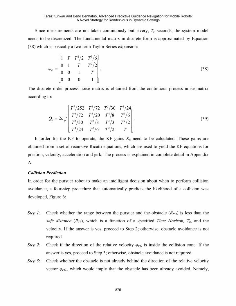
Collision Prediction

In order for the pursuer robot to make an intelligent decision about when to perform collision

avoidance, a four-step procedure that automatically predicts the likelihood of a collision was

developed, Figure 6:

Step 1: Check whether the range between the pursuer and the obstacle (RPO) is less than the

safe distance (RTh), which is a function of a specified Time Horizon, Th, and the

velocity. If the answer is yes, proceed to Step 2; otherwise, obstacle avoidance is not

required.

Step 2: Check if the direction of the relative velocity φPO is inside the collision cone. If the

answer is yes, proceed to Step 3; otherwise, obstacle avoidance is not required.

Step 3: Check whether the obstacle is not already behind the direction of the relative velocity

vector φPO,, which would imply that the obstacle has been already avoided. Namely,


875

check whether 1 1tan tan2 2

O P O PPO PO

O P O P

y y y yorx x x

π πϕ ϕ− ⎛ ⎞ ⎛− −≤ − ≥⎜ ⎟ ⎜− −⎝ ⎠ ⎝ x

− ⎞⎟⎠

. If the answer is

yes, proceed to Step 4; otherwise, obstacle avoidance is not required.

Step 4: Proceed to the obstacle- avoidance algorithm.

Is Range b/w pursuer and

obs RPO < RTh

Obstacle Avoidance

Reqd Is vPO inside

the CC? Is Obs in front

of pursuer?

Obstacle Avoidance Not Reqd

Yes Yes Yes

No No

No

Figure 6: Rules for Collision Prediction.

III. IMPLEMENTATION

In the proposed implementation strategy, for rendezvous with a moving target, the pursuer robot

receives its velocity command for the next time instant only from the APGL algorithm if obstacle

avoidance is not required, Figure 1. The pursuer proceeds in the direction generated by the

APGL, via aAPGL, which is only limited by the vehicle’s dynamic and kinematic characteristics.

Once in the vicinity of obstacles, however, the accelerations generated by the APGL algorithm

may need to be modified. Collision avoidance takes place based on evaluating the movement of

the pursuer and the obstacle. The procedure for generating the acceleration commands for the

next discrete time instance is discussed below.

Let us, for example, consider a dynamic environment shown in Figure 7a at a certain instant

in time ti. The pursuer has to rendezvous with a maneuvering target while avoiding a number of

dynamic obstacles. It is assumed that the obstacles have similar dynamic characteristics, in terms

of speed and maneuverability, as do the pursuer and the target. The procedure for generating the

desired acceleration commands for the pursuer is outlined below:


876

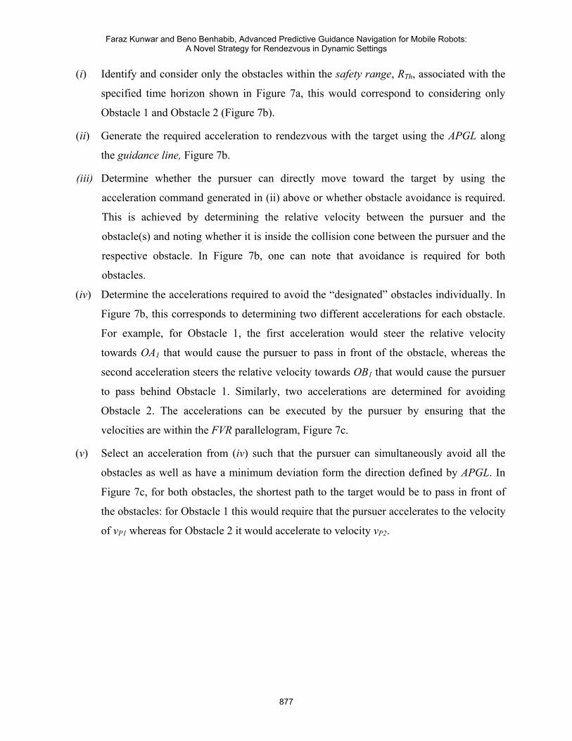
(i) Identify and consider only the obstacles within the safety range, RTh, associated with the

specified time horizon shown in Figure 7a, this would correspond to considering only

Obstacle 1 and Obstacle 2 (Figure 7b).

(ii) Generate the required acceleration to rendezvous with the target using the APGL along

the guidance line, Figure 7b.

(iii) Determine whether the pursuer can directly move toward the target by using the

acceleration command generated in (ii) above or whether obstacle avoidance is required.

This is achieved by determining the relative velocity between the pursuer and the

obstacle(s) and noting whether it is inside the collision cone between the pursuer and the

respective obstacle. In Figure 7b, one can note that avoidance is required for both

obstacles.

(iv) Determine the accelerations required to avoid the “designated” obstacles individually. In

Figure 7b, this corresponds to determining two different accelerations for each obstacle.

For example, for Obstacle 1, the first acceleration would steer the relative velocity

towards OA1 that would cause the pursuer to pass in front of the obstacle, whereas the

second acceleration steers the relative velocity towards OB1 that would cause the pursuer

to pass behind Obstacle 1. Similarly, two accelerations are determined for avoiding

Obstacle 2. The accelerations can be executed by the pursuer by ensuring that the

velocities are within the FVR parallelogram, Figure 7c.

(v) Select an acceleration from (iv) such that the pursuer can simultaneously avoid all the

obstacles as well as have a minimum deviation form the direction defined by APGL. In

Figure 7c, for both obstacles, the shortest path to the target would be to pass in front of

the obstacles: for Obstacle 1 this would require that the pursuer accelerates to the velocity

of vP1 whereas for Obstacle 2 it would accelerate to velocity vP2.


877

(a)

Pursuer

vP

vTvO1

vO2

vO3

vO4

vO5

Obs2 Obs5

Obs1

Obs3 Obs4

Target

RTh

(b)

vRO1

vRO2

Guidance Line

Obs1

Obs2 O Pursuer

A1

B1

B2

vO1

-vO1 vO2-vO2vP

A2

(c)

vP2

vP1

vRO1

vRO2

Obs1

Pursuer

Guidance Line

Avoidance Cone

Obs2

(d)

vO1

vO2

vP

Obs1

Obs2

Pursuer

Guidance Line

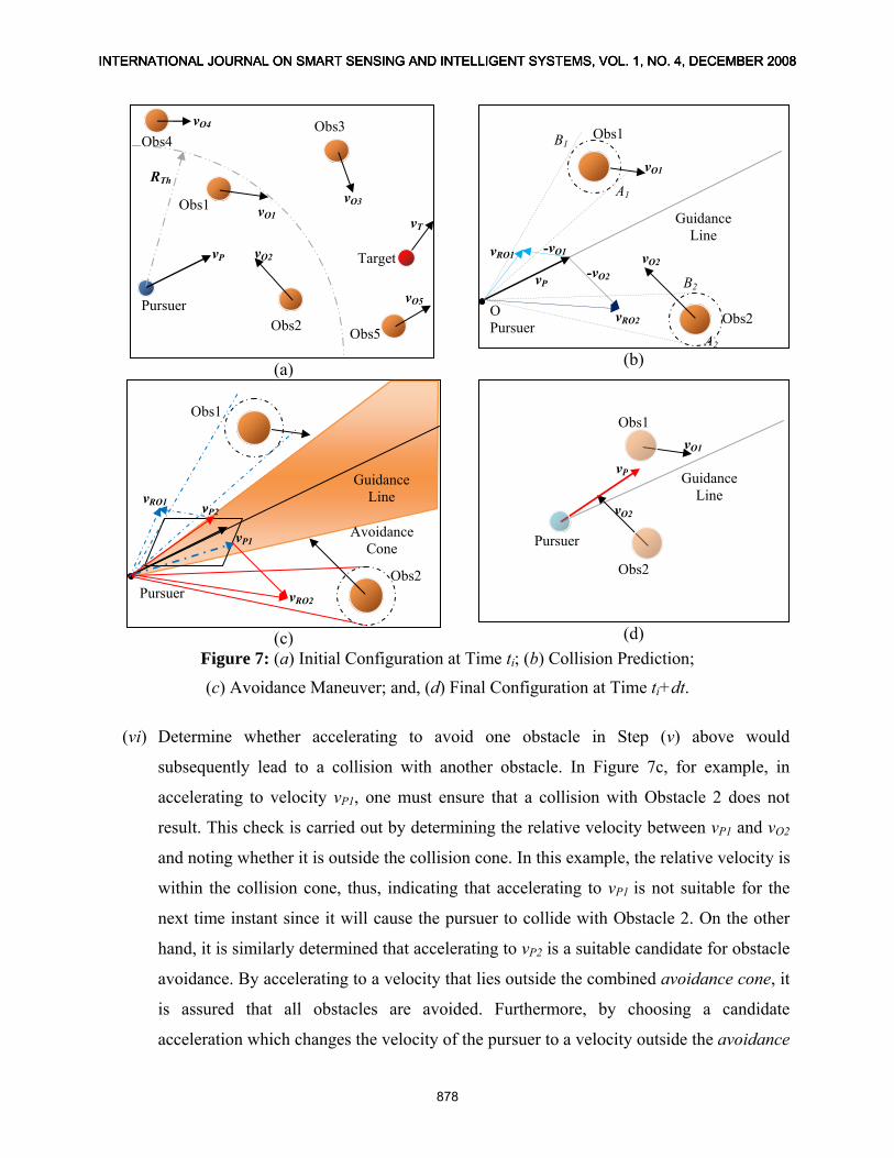
Figure 7: (a) Initial Configuration at Time ti; (b) Collision Prediction;

(c) Avoidance Maneuver; and, (d) Final Configuration at Time ti+dt.

(vi) Determine whether accelerating to avoid one obstacle in Step (v) above would

subsequently lead to a collision with another obstacle. In Figure 7c, for example, in

accelerating to velocity vP1, one must ensure that a collision with Obstacle 2 does not

result. This check is carried out by determining the relative velocity between vP1 and vO2

and noting whether it is outside the collision cone. In this example, the relative velocity is

within the collision cone, thus, indicating that accelerating to vP1 is not suitable for the

next time instant since it will cause the pursuer to collide with Obstacle 2. On the other

hand, it is similarly determined that accelerating to vP2 is a suitable candidate for obstacle

avoidance. By accelerating to a velocity that lies outside the combined avoidance cone, it

is assured that all obstacles are avoided. Furthermore, by choosing a candidate

acceleration which changes the velocity of the pursuer to a velocity outside the avoidance


878

cone closest to the rendezvous velocity obtained from APGL provides the desired optimal

velocity for the next time instant. In this example, it is vP2, which would cause the robot

to pass in front of Obstacle 2, but, behind Obstacle 1, Figure 7d.

A primary advantage of using the above procedure is the consideration of only the obstacles

that would potentially collide with the pursuer while obtaining a time-optimal trajectory. Thus,

the acceleration of the pursuer aP for the next time instant (ti+dt) is given by:

( ) i

if obstacle avoidance is not required

if obstacle avoidance is required.t dt

⎧+ = ⎨

⎩APGL

POANL

aa

a . (40)

IV. SIMULATIONS

A number of simulations were carried out using the proposed APGL-based algorithm, Table 1:

the maximum velocity and lateral acceleration of the pursuer robot was limited to 200 mm/s and

2000 mm/s2, respectively, in all the examples, and the criterion for successful rendezvous was set

to <10 mm relative distance in both X and Y directions and a relative velocity of <10 mm/s.

Furthermore, in order to examine the effect of noise on the performance of the proposed

algorithm, simulated noise (up to 5%) was added to the target’s “measured” position: 1% noise is

equivalent to about 10 mm in robot travel.

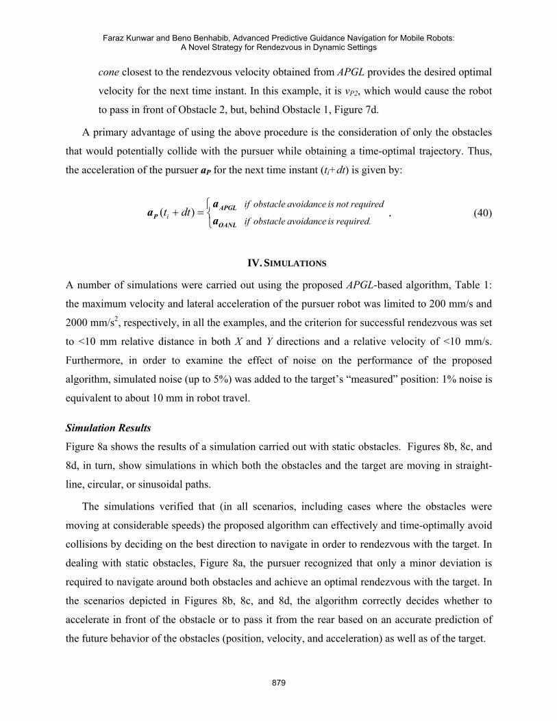
Simulation Results

Figure 8a shows the results of a simulation carried out with static obstacles. Figures 8b, 8c, and

8d, in turn, show simulations in which both the obstacles and the target are moving in straight-

line, circular, or sinusoidal paths.

The simulations verified that (in all scenarios, including cases where the obstacles were

moving at considerable speeds) the proposed algorithm can effectively and time-optimally avoid

collisions by deciding on the best direction to navigate in order to rendezvous with the target. In

dealing with static obstacles, Figure 8a, the pursuer recognized that only a minor deviation is

required to navigate around both obstacles and achieve an optimal rendezvous with the target. In

the scenarios depicted in Figures 8b, 8c, and 8d, the algorithm correctly decides whether to

accelerate in front of the obstacle or to pass it from the rear based on an accurate prediction of

the future behavior of the obstacles (position, velocity, and acceleration) as well as of the target.


879

Table 1: Summary of Simulation Data. Obstacle 1 Obstacle 2 Target

S.No Type Max. Vel

(mm/s) Type Max. Vel(mm/s) Type Max. Vel

(mm/s)

Rendezvous Time (s)

1 Static 0 Static 0 Sinusoidal 120 8.2 2 Straight 150 Straight 150 Straight 130 7.9 3 Circular 150 Circular 100 Sinusoidal 110 8.8 4 Sinusoidal 180 Sinusoidal Sinusoidal 170 120 8.5

(a)

(b)

(d) (c)

Figure 8: Simulations with (a) Static Obstacles, (b) Obstacles and Target Moving in Straight

Lines, (c) Obstacles Moving on Circular Paths, and (d) Obstacles Moving Sinusoidally.

V. EXPERIMENTS

The physical layout of the experimental set-up is depicted in Figure 9 and the hardware

specifications are given in Table 2. The software for the experiments, running on a Pentium IV

1.6 GHz processor PC, consisted of three modules: image acquisition and processing, trajectory

planning, and communication modules, respectively. An analog CCD camera captured the image


880

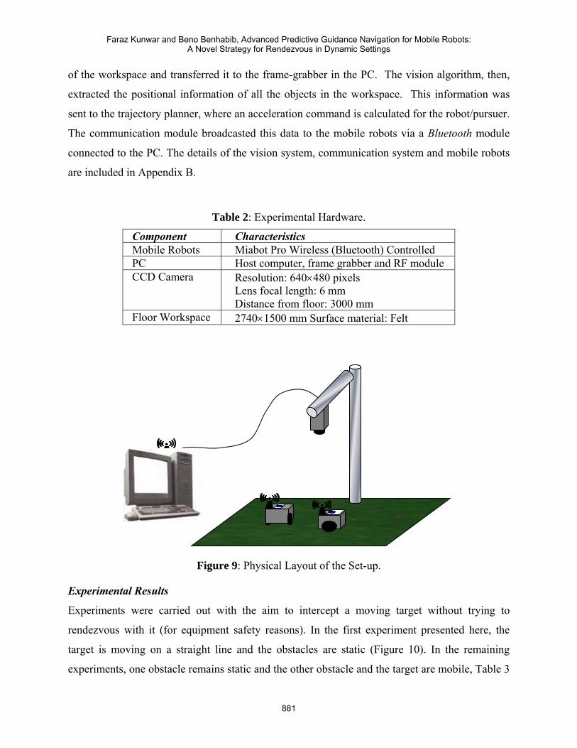
of the workspace and transferred it to the frame-grabber in the PC. The vision algorithm, then,

extracted the positional information of all the objects in the workspace. This information was

sent to the trajectory planner, where an acceleration command is calculated for the robot/pursuer.

The communication module broadcasted this data to the mobile robots via a Bluetooth module

connected to the PC. The details of the vision system, communication system and mobile robots

are included in Appendix B.

Table 2: Experimental Hardware.

Component Characteristics Mobile Robots Miabot Pro Wireless (Bluetooth) Controlled PC Host computer, frame grabber and RF module CCD Camera Resolution: 640×480 pixels

Lens focal length: 6 mm Distance from floor: 3000 mm

Floor Workspace 2740×1500 mm Surface material: Felt

Figure 9: Physical Layout of the Set-up.

Experimental Results

Experiments were carried out with the aim to intercept a moving target without trying to

rendezvous with it (for equipment safety reasons). In the first experiment presented here, the

target is moving on a straight line and the obstacles are static (Figure 10). In the remaining

experiments, one obstacle remains static and the other obstacle and the target are mobile, Table 3


881

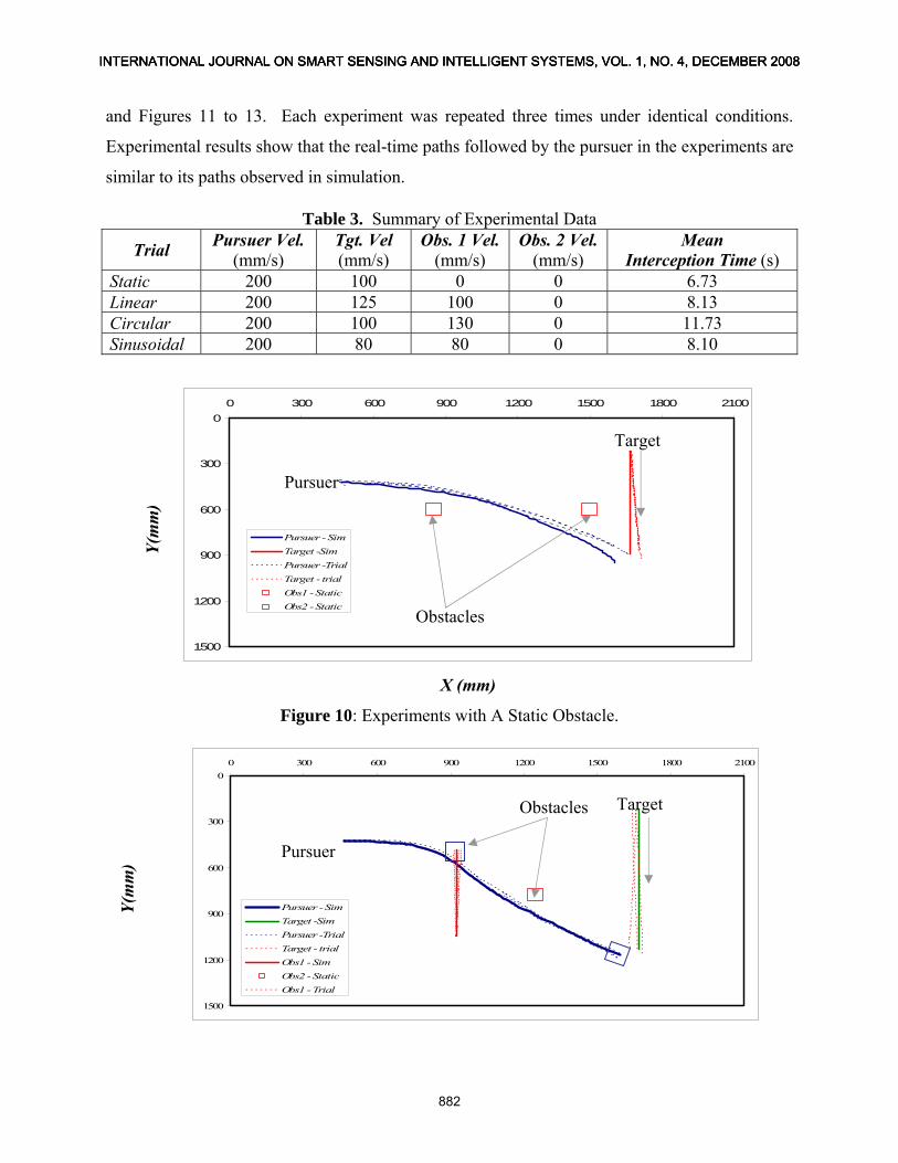
and Figures 11 to 13. Each experiment was repeated three times under identical conditions.

Experimental results show that the real-time paths followed by the pursuer in the experiments are

similar to its paths observed in simulation.

Table 3. Summary of Experimental Data

Trial Pursuer Vel. (mm/s)

Tgt. Vel (mm/s)

Obs. 1 Vel. (mm/s)

Obs. 2 Vel. (mm/s)

Mean Interception Time (s)

Static 200 100 0 0 6.73 Linear 200 125 100 0 8.13 Circular 200 100 130 0 11.73 Sinusoidal 200 80 80 0 8.10

Y(m

m)

0

300

600

900

1200

1500

0 300 600 900 1200 1500 1800 2100

Pursuer - SimTarget -SimPursuer -TrialTarget - trialObs1 - StaticObs2 - Static

Target

Pursuer

Obstacles

X (mm)

Figure 10: Experiments with A Static Obstacle.

Y(m

m)

0

300

600

900

1200

1500

0 300 600 900 1200 1500 1800 2100

Pursuer - SimTarget -SimPursuer -TrialTarget - trialObs1 - SimObs2 - StaticObs1 - Trial

Target Obstacles

Pursuer


882

X (mm)

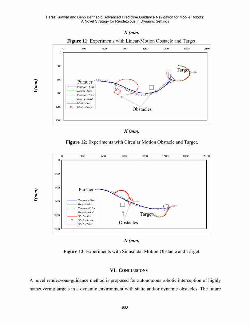
Figure 11: Experiments with Linear-Motion Obstacle and Target.

0

300

600

900

1200

1500

0 300 600 900 1200 1500 1800 2100

Pursuer - SimTarget -SimPursuer -TrialTarget - trialObs1 - SimObs2 - Static

Target

Y(m

m) Pursuer

Obstacles

X (mm)

Figure 12: Experiments with Circular Motion Obstacle and Target.

0

300

600

900

1200

1500

0 300 600 900 1200 1500 1800 2100

Pursuer - SimTarget -SimPursuer -TrialTarget - trialObs1 - SimObs2 - StaticObs1 - Trial

Pursuer

Y(m

m)

Target

Obstacles

X (mm)

Figure 13: Experiments with Sinusoidal Motion Obstacle and Target.

VI. CONCLUSIONS

A novel rendezvous-guidance method is proposed for autonomous robotic interception of highly

maneuvering targets in a dynamic environment with static and/or dynamic obstacles. The future


883

maneuver of the target is predicted using a five-state Extended Kalman Filter (EKF). The

proposed algorithm, then, uses the novel Advanced Predictive Guidance Law (APGL) to obtain

the required acceleration commands for rendezvous with the target. In the presence of obstacles,

the algorithm uses the novel Obstacle-Avoidance Navigation Law (OANL), which first predicts

the likelihood of a collision and, then defines a collision cone for each potentially colliding

obstacle (within close proximity of) the pursuer. Based on this information the algorithm directs

the relative velocity between the pursuer and the obstacle outside the collision cone. By

employing a velocity and heading outside the collision cone, a collision-free trajectory to the

target is ensured. EKF is also used to track the obstacles states.

Furthermore, in our algorithm, instead of using some form of a heuristic search strategy,

proposed in most obstacle-avoidance techniques, the search for a feasible velocity for the next

sampling interval is reduced to velocities that are as close to the maximum closing velocity

component obtained from the APGL method as possible.

Simulations and experiments have verified the system to be efficient and robust in regards to

interception of moving targets with various different interception parameters and situations.

REFERENCES [1] F. Kunwar, F. Wong, R. Ben Mrad, and B. Benhabib, “Rendezvous Guidance for The Autonomous

Interception of Moving Objects in Cluttered Environments,” IEEE Conference on Robotics and Automation, pp. 3787-3792, Barcelona, Spain, April 2005.

[2] F. Kunwar, F. Wong, R. Ben Mrad, and B. Benhabib, “Time-Optimal Rendezvous with Moving Objects in Dynamic Cluttered Environments Using A Guidance Based Technique,” IEEE International Conference on Intelligent Robots and Systems, pp. 283-288, Edmonton, Canada, August 2005.

[3] Zarchan P., Tactical and Strategic Missile Guidance, Fourth Edition, American Institute of Aeronautics and Astronautics, Virginia, 2003.

[4] H. L. Pastrick, S. M. Seltzer, and M. E. Warren, “Guidance Laws for Short-Range Tactical Missiles,” Journal of Guidance, Control and Dynamics, Vol. 4, No. 2, pp. 98-108, 1981.

[5] G. M. Anderson, “Comparison of Optimal Control and Differential Game Intercept Missile Guidance Law” AIAA Journal of Guidance and Control, Vol. 4, No. 2, pp.109-115, March 1981.

[6] D. Ghose, “True Proportional Navigation with Manoeuvring Target,” IEEE Transactions on Aerospace and Electronic Systems, Vol. 1, No. 30, pp. 229-237, January 1994.

[7] T. J. Speyer, K. Kim, and M. Tahk, “Passive Homing Missile Guidance Law Based on New Target Maneuver Models,” Journal of Guidance, Vol. 1, No. 13, pp. 803-812, September 1990.

[8] C. D. Yang, and C. C. Yang, “A Unified Approach to Proportional Navigation,” IEEE, Transactions on Aerospace and Electronic Systems, Vol. 33, No. 2, pp. 557-567, 1997.

[9] P. J. Yuan, and S. C. Hsu, “Rendezvous Guidance with Proportional Navigation,” Journal of Guidance, Control, and Dynamics, Vol. 17, No. 2, pp. 409-411, 1993.

[10] M. Guelman, “Guidance for Asteroid Rendezvous,” Journal of Guidance, Control, and Dynamics, Vol. 14, No. 5, pp. 1080-1083, 1990.


884

[11] D. L. Jensen, “Kinematics of Rendezvous Manoeuvres,” Journal of Guidance, Vol. 7, No. 3, pp. 307-314, 1984

[12] M. Mehrandezh, M. N. Sela, R. G. Fenton, and B. Benhabib, “Robotic Interception of Moving Objects Using an Augmented Ideal Proportional Navigation Guidance Technique,” IEEE, Transactions on Systems, Man and Cybernetics, Vol. 30, No. 3, pp. 238-250, 2000.

[13] J. M. Borg, M. Mehrandezh, R. G. Fenton, and B. Benhabib, “Navigation-Guidance-Based Robotic Interception of Moving Objects in Industrial Settings,” Journal of Intelligent and Robotic Systems, Vol. 33, No. 1, pp. 1-23, 2002.

[14] F. Agah, M. Mehrandezh, R. G. Fenton, and B. Benhabib, “On-line Robotic Interception Planning Using Rendezvous-Guidance Technique,” Journal of Intelligent and Robotic Systems: Theory and Applications, Vol. 40, No. 1, pp. 23-44, May 2004.

[15] U. Ghumman, F. Kunwar, and B. Benhabib, “Guidance-Based On-Line Motion Planning for Autonomous Highway Overtaking,” International Journal on Smart Sensing and Intelligent Systems, Vol. 1, No. 2, pp. 589-571, June 2008.

[16] Latombe, J.C., Robot Motion Planning, Boston: Kluwer Academic Publishers, 1991. [17] J. Baraquand, B. Langlois, and J. C. Latombe, “Numerical Potential Field Techniques for Robot Path

Planner,” IEEE, Transactions on Systems, Man and Cybernetics, Vol. 22, No. 2, pp. 224-241, March-April 1992.

[18] J. Borenstein, and Y. Koren “The Vector Field Histogram – Fast Obstacle Avoidance for Mobile Robot,” IEEE Journal of Robotics and Automation, vol. 7, no. 3, pp. 278-288, June 1991’

[19] J.P. Laumond, P.E. Jacobs, M. Taix, and R.M. Murray, “A Motion Planner for Nonholonomic Mobile Robots,” IEEE Transactions on Robotics and Automation, Vol. 10, No. 5, pp. 577-593, October 1994.

[20] Laumond, J.P., Robot Motion Planning and Control, Springer-Verlag Telos, 1998. [21] R. Simmons, “The Curvature-Velocity Method for Local Obstacle Avoidance”, IEEE International

Conference on Robotics and Automation, pp. 2275-2282, Minneapolis, MN, April 1996. [22] D. Fox, W. Burgard, and S. Thrun, “The Dynamic Window Approach to Collision Avoidance,” IEEE

Robotics and Automation Magazine, Vol. 4. No.1, pp. 23-33, March 1997. [23] W. Feiten, R. Bauer, and G. Lawitzky, “Robust Obstacle Avoidance in Unknown and Cramped

Environments,” IEEE International Conference on Robotics and Automation, pp. 2412-241, May 1994. [24] F. Zhang, A. O’Conner, D. Luebke, and P.S. Krishnaprasad, “The Experimental Study of Curvature-Based

Control Laws for Obstacle Avoidance,” IEEE International Conference on Robotics and Automation, Vol. 4, pp. 3849-3854, New Orleans, LA, April, 2004.

[25] N.Y. Ko and R.G. Simmons. “The Lane-Curvature Method for Local Obstacle Avoidance,” IEEE Conference on Intelligent Robots and Systems, pp. 1615- 1621 Victoria, Canada, October 1998.

[26] P. Ogren and N.E. Leonard, “A Tractable Convergent Dynamic Window Approach to Obstacle Avoidance,” IEEE International Conference on Intelligent Robots and Systems, pp. 595-600, Lausanne, Switzerland, September 2002.

[27] H. Hu and M. Brady, “A Bayesian Approach to Real-time Obstacle Avoidance for Mobile Robots,” Autonomous Robots, Vol. 1, pp. 69-92, January 1994.

[28] D. Fox, W. Burgard., S. Thrun and A. Cremers, “A Hybrid Collision Avoidance Method for Mobile Robots”, IEEE International Conference on Robotics and Automation, pp. 1238-1243, 1998.

[29] P. Fiorini and Z. Shiller, “Motion Planning in Dynamic Environments using Velocity Obstacles,” International Journal on Robotics Research, Vol. 17, No. 7, pp. 711-727, 1998.

[30] F. Large, S. Sekhavat, Z. Shiller,and C. Laugier, “Towards Real-Time Global Motion Planning in a Dynamic Environment Using the NLVO Concept,” IEEE International Conference on Intelligent Robots and Systems, pp. 607-612, Lausanne, Switzerland, 2002.

[31] Z. Li, J. Canny, J. and G. Heinzinger, “Robot Motion Planning with Non-Holonomic Constraints.” 5th International Symposium of Robotics Research, pp. 343-350. Tokyo, Japan, 1989.


885

[32] P. Rouchen, M. Fliess, J. Levine, and P. Martin, “Flatness and Motion Planning: the Car with n Trailers,” European Control Conference, pp. 1518-1522, 1992.

[33] R. M. Murray and S. S. Sastry, “Nonholonomic Motion Planning: Steering Using Sinusoids,’’ IEEE, Transactions on Automatic Control, Vol. 38, pp. 700-716, 1993.

[34] S. Monaco and D. Normand-Cyrot, “An Introduction to Motion Planning under Multirate Digital Control,” IEEE Conference on Decision and Control, Tucson, Arizona, pp. 1780-1785, December 1992.

[35] D. Elbury, R. M. Murray, and S. S. Sashy, “Trajectory Generation for the n-Trailer Problem Using Goursat Normal Form,” IEEE, Transactions on Automatic Control, Vol. 40, pp. 802-819, 1995.

[36] C. Fernandes, L. Gurvits, and 2. Li, “Near-optimal Nonholonomic Motion Planning for A System of Coupled Rigid Bodies,” IEEE, Transactions on Automatic Control, Vol. 39, pp. 450463, 1994.

[37] D. J. Balkcom, and M. T. Mason, “Extrema1 Trajectories for Bounded Velocity Differential Drive Robots,” IEEE International Conference on Robotics & Automation, pp. 1747-1752, California, April 2000.

[38] D. J. Balkcom, and M. T. Mason, “Extrema1 Trajectories for Bounded Velocity Mobile Robots,” IEEE International Conference on Robotics & Automation, pp. 1747-1752, Washington, DC, May 2002.

[39] S. Sundar and Z. Shiller, “Optimal Obstacle Avoidance Based on the Hamilton-Jacobi-Bellman Equation,” IEEE, Transactions on Robotics and Automation. Vol. 13, pp. 305-310, 1997.

[40] A. E. Bryson and Y.-C. Ho, Applied Optimal Control, 2nd Edition, Hemisphere Publishing Corporation, New York, 1975.

[41] Z. Qu and J. R. Cloutier, “A New Suboptimal Control Design for Cascaded Nonlinear Systems,” Optimal Control: Applications and Methods, vol. 23, pp. 303-328, 2002.

[42] J.-P. Laumond, P. E. Jacobs, M. Taix, and R. M. Murray, “A Motion Planner for Nonholonomic Mobile Robots,” IEEE Transactions on Robotics and Automation, Vol. 10, pp. 577-593, 1994.

[43] J. A. Reeds and R. A. Shepp, “Optimal Paths for a Car that Goes Both Forward and Backwards,” Pacific J. Mathematics, Vol. 145, pp. 367-393, 1990.

[44] P. Vadekkapat, and D. Goswami, “Biped Locomotion: Stability Analysis and Control,” International Journal on Smart Sensing and Intelligent Systems, Vol. 1, No.1, pp. 589-571, March 2008.

[45] A. Chakravarthy and D. Ghose, “Obstacle Avoidance in a Dynamic Environment: A Collision Cone Approach,” IEEE Transactions On Systems, Man, And Cybernetics—Part A: Systems And Humans, Vol. 28, No. 5, September 1998.

[46] D. Bourgin, “Color Space FAQ,” http://www.neuro.sfc.keio.ac.jp/~aly /polygon/info/ color-space-faq.html, August 2004.

[47] C.B. Bose and J. Amir, “Design of Fiducials For Accurate Registration Using Machine Vision,” IEEE, Transactions on Pattern Analysis and Machine Intelligence, Vol. 12, No. 12, pp. 1196-1200, December 1990.

APPENDIX A: EXTENDED KALMAN FILTER

The Kalman filter is a two-step probabilistic estimation process that is very popular in the

robotics world as a tool to predict the next position of the robot in a linear system. Kalman filters

are based on linear algebra and the hidden Markov model. The underlying dynamical system is

modeled as a Markov chain built on linear operators perturbed by Gaussian noise. The state of

the system is represented as a vector of real numbers. At each discrete time increment, a linear

operator is applied to the state to generate the new state, with some noise mixed in, and


886

optionally some information from the controls on the system if they are known. Then, another

linear operator mixed with more noise generates the visible outputs from the hidden state. The

Kalman filter is a recursive estimator. This means that only the estimated state from the previous

time step and the current measurement are needed to compute the estimate for the current state.

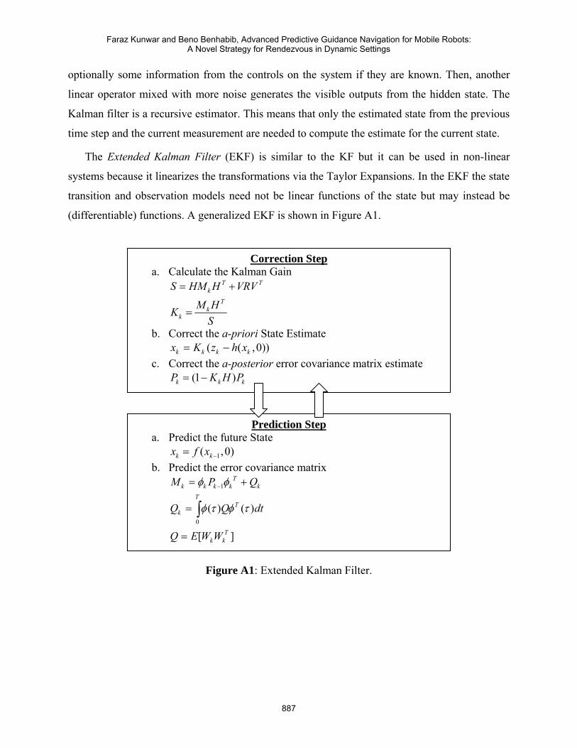
The Extended Kalman Filter (EKF) is similar to the KF but it can be used in non-linear

systems because it linearizes the transformations via the Taylor Expansions. In the EKF the state

transition and observation models need not be linear functions of the state but may instead be

(differentiable) functions. A generalized EKF is shown in Figure A1.

Correction Step a. Calculate the Kalman Gain

T Tk

Tk

k

S HM H VRV

M HKS

= +

=

b. Correct the a-priori State Estimate ( ( ,0))k k k kx K z h x= − c. Correct the a-posterior error covariance matrix estimate (1 )k k kP K H P= −

Prediction Step a. Predict the future State 1( ,0)k kx f x −= b. Predict the error covariance matrix

1

0

( ) ( )

[ ]

Tk k k k k

TT

k

Tk k

M P Q

Q Q dt

Q E W W

φ φ

φ τ φ τ

−= +

=

=

∫

Figure A1: Extended Kalman Filter.


887

Notation x state estimate z measurement data φ Jacobian of the system model with respect to state W Jacobian of the system model with respect to process noise V Jacobian of measurement model with respect to measurement noise H Jacobian of the measurement model Q process noise covariance R measurement noise covariance K Kalman Gain P estimated error covariance σp prediction noise σm measurement noise

APPENDIX B: DETAILS OF THE EXPERIMENTAL SET-UP

B1. Vision System

The robot, the obstacles, and the target were color-coded for identification. The raw image

containing three channels of data, indicating the intensities of the Red (R), Green (G) and Blue

(B) colors, in each pixel were transformed into the YCbCr (luminance, chrominance-blue, and

chrominance-red) color space. The transformation is performed by [47]:

(B1) 0.299 0.587 0.114Y R G= + + B

2 , (B2) ( ) /1.77Cb B Y= −

(B3) ( ) /1.402Cr R Y= −

where Y has a range of [0, 255] and Cb and Cr both have a range of [−127.5, 127.5].

When an image is examined, the weighted Euclidean distances, in the YCbCr color space,

between each pixel in the image and the predefined colour set are calculated: 2 20.15( ) 0.425( ) 0.425( )p c p c p c

2D Y Y Cb Cb Cr Cr= − + − + − , (B4)

where D is the weighted Euclidean distance, Yp, Cbp, and Crp, are the measured YCbCr values of

the pixel, and Yc, Cbc, and Crc are the values of the predefined color set. During the experiments,

it was noted that the pixels on the identification marker did not vary more than 18.0 in weighted

Euclidean distance from the defined YCbCr value. This value was, therefore, set as the threshold


888

distance: if a pixel is within this threshold distance of a certain color in the predefined color set,

then, it is considered to be that color. After the image has gone through the thresholding

operation, the positions of the mobile robot, the obstacles, and the target are determined.

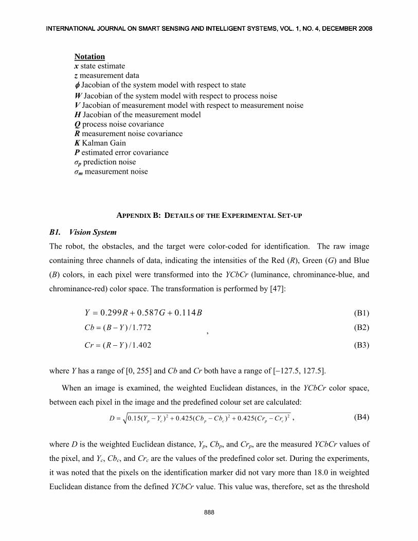
A search is performed to find the markers on all the objects. In order to achieve the smallest

sampling rate, the dimension of the smallest marker is used, denoted here as l pixels. Starting

from the pixel location (0, 0), every 0.5l pixels are sampled along the X and Y directions. If the

sampled pixel has the color of the predefined set, a search frame is placed over that pixel. The

size of the search frame is twice the diameter of the marker. If the number of pixels of a certain

color in the search frame exceeds a pre-determined threshold, then, a marker of that color is

considered to be located in that search frame. The centroid of that color blob is, then, calculated

to sub-pixel accuracy using the Centroid Method [46], Figure B1.

With all the markers located, object identification can be performed. The vision program first

searches for blue markers. Once a blue marker is found, the algorithm looks for a white marker

within a distance of the radius of a robot. If a corresponding white marker is located, then, a

robot has been successfully identified. Bearing of the object is indicated by an imaginary line

drawn from the centre of the blue circle to the centroid of the white pattern. The algorithm takes

approximately 150 ms to execute (i.e., a frame-rate of 6.5 fps).

D

Search Frame

Sampling Points

Colour of Interest

Sampled Point - Colour of

Predefined Set

Robot Marked Pattern l

Workspace

Figure B1: Color Marker Search.


889

B2. Communication System

The Bluetooth card enables the robot to communicate with the host PC, converting the Bluetooth

link to logic-level serial signals. The MIABOT-BT Bluetooth boards are supplied with fixed

communication settings 19200 baud (8 bits, 1 stop bit, no parity). A PC Bluetooth dongle is

supplied that plugs into the USB port on the PC. This can support wireless links with up to 7

robots at once.

B3. Mobile Robots

Three Miabot PRO BT v2 differential-drive mobile robots were used in the implementation of

the proposed methodology: a pursuer, a moving obstacle, and a target. The robot motors are

driven by 6×1.2 V (AA) cells through a low-resistance driver I.C. with a slow-acting current

limit at about 5A. Maximum speed of an unloaded motor is in the region of 6000 to 8000 rpm.

The motor shafts drive the wheels through an 8:1 gearing. The motors incorporate quadrature

encoders giving 512 position-pulses per rotation. The wheels are 52mm in diameter; one encoder

pulse corresponds to just under 0.04 mm of movement. Each robot contains two 3 AA-cell

battery packs (nominal 1.2V per cell, 1300 mAh).

ACKNOWLEDGMENTS

We acknowledge the support of the Natural Sciences and Engineering Research Council of

Canada (NSERC).


890

Documents

Advanced Predictive Guidance Navigation for Mobile …s2is.org/Issues/v1/n4/papers/paper3.pdf · · 2016-03-02Advanced Predictive Guidance Navigation for Mobile Robots: ... Advanced