Advanced photoacoustic image reconstruction using the · PDF fileAdvanced photoacoustic image reconstruction using the ... Super cially, this would ... All of the algorithms discussed

Advanced photoacoustic image reconstruction using thek-Wave toolbox

B. E. Treeby∗, J. Jaros†, and B. T. Cox∗

∗Department of Medical Physics and Biomedical Engineering, University College London, UK†Faculty of Information Technology, Brno University of Technology, Czech Republic

ABSTRACT

Reconstructing images from measured time domain signals is an essential step in tomography-mode photoa-coustic imaging. However, in practice, there are many complicating factors that make it difficult to obtainhigh-resolution images. These include incomplete or undersampled data, filtering effects, acoustic and opti-cal attenuation, and uncertainties in the material parameters. Here, the processing and image reconstructionsteps routinely used by the Photoacoustic Imaging Group at University College London are discussed. Theseinclude correction for acoustic and optical attenuation, spatial resampling, material parameter selection, imagereconstruction, and log compression. The effect of each of these steps is demonstrated using a representativein vivo dataset. All of the algorithms discussed form part of the open-source k-Wave toolbox (available fromhttp://www.k-wave.org).

1. INTRODUCTION

Forming an image from measured time domain signals is an essential step in photoacoustic tomography (PAT).Superficially, this would appear to be a solved problem, particularly given the large number of publishedphotoacoustic images.1 Indeed, commercial photoacoustic scanners are now available that can generate imagesin real time,2 and exact reconstruction formulae for canonical geometries have existed in the mathematicalliterature for some time.3 However, in the practical case, there are many complicating factors that make itdifficult to obtain high-resolution images with good signal-to-noise. These include the data being incomplete(e.g., because the detection aperture is limited or spatially undersampled),4 filtering effects (e.g., because thetransducer elements have limited sensitivity and bandwidth, and have a finite size),5, 6 limited penetrationdepth (due to optical and acoustic attenuation),1, 7 and uncertainties in the material properties needed for thereconstruction.8, 9 While advances have been made to address many of these challenges, the rapid growth inthe development and application of photoacoustic technology means that there is often a disconnect betweenresearchers developing new algorithms and those performing in vivo imaging studies. In this paper, the pre-processing, image reconstruction, and post-processing steps routinely used by the Photoacoustic Imaging Groupat University College London (UCL) to generate high-resolution photoacoustic images are discussed. Thepurpose is to provide insight into the impact of applying different techniques on reconstructed photoacousticimages. All of the algorithms discussed form part of the open-source k-Wave image reconstruction toolboxdeveloped at UCL (available from http://www.k-wave.org).10 This makes it easy for other researchers toapply them to their own datasets.

2. DATASET AND ACQUISITION PARAMETERS

The dataset used to demonstrate the different image reconstruction steps is taken from Ref. 11 (see Fig. 3(f)and front cover). This is an in vivo dataset of the blood vasculature and a xenograft (or tumour) composed ofK562 cells labelled with a tyrosinase-based genetic reporter taken in the flank of a nude mouse. The dataset wasacquired using a photoacoustic scanning system based on a planar Fabry-Perot interferometer.12 This was usedas a 2D detection array with 142 × 141 detection elements (giving a total of 20,022 time domain waveforms), anelement separation of 100 µm (giving a scan area of 14.2 × 14.1 mm), and an optically defined element size of22 µm.11 The -3 dB bandwidth of the detection system was 0.35−22 MHz, and the three-sigma noise equivalent

Send correspondence to [email protected].

Photons Plus Ultrasound: Imaging and Sensing 2016, edited by Alexander A. Oraevsky, Lihong V. WangProc. of SPIE Vol. 9708, 97082P · © 2016 SPIE · CCC code: 1605-7422/16/$18 · doi: 10.1117/12.2209254

Proc. of SPIE Vol. 9708 97082P-1

Downloaded From: http://spiedigitallibrary.org/ on 03/19/2016 Terms of Use: http://spiedigitallibrary.org/ss/TermsOfUse.aspx

Time [µs]

x−p

osi

tio

n [

mm

]

0 1 2 3 4 5

0

2

4

6

8

10

12

14 −1

−0.5

0

0.5

1

Time [µs]

Fre

qu

en

cy [

MH

z]

0 1 2 3 4 50

5

10

15

20

[dB]

[au]

−40

−35

−30

−25

−20

−15

−10

−5

0

Time [µs]

x−p

osi

tio

n [

mm

]

0 1 2 3 4 5

0

2

4

6

8

10

12

14

0 5 10 15 20 25−30

−25

−20

−15

−10

−5

0

5

Po

we

r S

pe

ctru

m [

dB

]

Frequency [MHz]

(a)

(c)

(b)

(d)

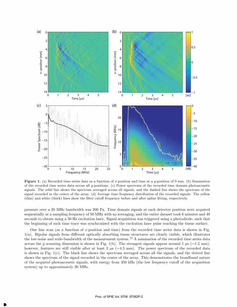
Figure 1. (a) Recorded time series data as a function of x-position and time at a y-position of 9 mm. (b) Summationof the recorded time series data across all y-positions. (c) Power spectrum of the recorded time domain photoacousticsignals. The solid line shows the spectrum averaged across all signals, and the dashed line shows the spectrum of thesignal recorded in the centre of the array. (d) Average time frequency distribution of the recorded signals. The yellow(thin) and white (thick) lines show the filter cutoff frequency before and after spline fitting, respectively.

pressure over a 20 MHz bandwidth was 200 Pa. Time domain signals at each detector position were acquiredsequentially at a sampling frequency of 50 MHz with no averaging, and the entire dataset took 6 minutes and 40seconds to obtain using a 50 Hz excitation laser. Signal acquisition was triggered using a photodiode, such thatthe beginning of each time trace was synchronised with the excitation laser pulse reaching the tissue surface.

One line scan (as a function of x-position and time) from the recorded time series data is shown in Fig.1(a). Bipolar signals from different optically absorbing tissue structures are clearly visible, which illustratesthe low-noise and wide-bandwidth of the measurement system.12 A summation of the recorded time series dataacross the y scanning dimension is shown in Fig. 1(b). The strongest signals appear around 1 µs (∼1.5 mm),however, features are still visible after at least 3 µs (∼4.5 mm). The power spectrum of the recorded datais shown in Fig. 1(c). The black line shows the spectrum averaged across all the signals, and the dotted lineshows the spectrum of the signal recorded in the centre of the array. This demonstrates the broadband natureof the acquired photoacoustic signals, with energy from 350 kHz (the low frequency cutoff of the acquisitionsystem) up to approximately 20 MHz.



3. IMAGE RECONSTRUCTION AND PROCESSING STEPS

3.1. Workflow

The pre-processing, reconstruction, and post-processing steps used to reconstruct the dataset shown in Fig. 1are outlined below. The same procedure is routinely followed for most recent in vivo imaging studies using theFabry-Perot scanner published by the Photoacoustic Imaging Group at UCL, e.g., Refs. 13–15.

1. Correct for acoustic attenuation in the time series data

2. Select sound speed that maximises the sharpness of the reconstructed image

3. Spatially upsample the acquired data to improve image resolution

4. Reconstruct the photoacoustic image

5. Correction for optical attenuation in the image data

6. Apply image processing and segmentation techniques as appropriate

7. Display as maximum intensity projection (MIP)

These steps are discussed in the following sections, with further details given in the references. The MATLABand k-Wave functions used to perform these steps are also described. Note, to illustrate the effect of the indi-vidual steps on the final reconstructed image, the images displayed in each section are reconstructed cognisantof details discussed in other sections. In particular, the optimum sound speed is always used, except whereotherwise noted.

3.2. Acoustic attenuation compensation

It is well known that soft biological tissue is acoustically absorbing, with the experimentally observed attenu-ation following a frequency power law of the form α = α0f

y. Due to the broadband nature of the ultrasoundwaves generated in photoacoustics, this causes a depth-dependent magnitude error and blurring of featuresin the reconstructed image. Applying compensation for acoustic attenuation can correct for these errors andimprove the visibility and resolution of deeper vessels.16, 17 Here, attenuation compensation is performed usingtime-variant filtering, which applies the correction directly to the time series data before reconstruction.18 Thisapproach is very flexible, and can be applied regardless of the acquisition system, geometry, or the reconstruc-tion method used. The algorithm works by applying a non-stationary convolution matrix to each recordedtime series patt, where pcorr(t1)

...pcorr(tN )

=

F (t1, τ1) . . . F (t1, τN )...

...F (tN , τ1) . . . F (tN , τN )

patt(τ1)

...patt(τN )

. (1)

The matrix F is constructed to allow attenuation compensation as a function of both frequency and traveldistance (or time).18 In k-Wave, this is applied using the function attenComp

sensor_data = attenComp(sensor_data, dt, c0, a0, y);

where sensor_data is a 2D matrix containing the recorded time series patt in each row, dt is the size of thetime step in units of s, c0 is the sound speed in units of m/s, a0 is the power law absorption prefactor in unitsof dB/(MHzy cm), and y is the power law absorption exponent. This function also automatically selects acutoff frequency for the attenuation compensation (to stop high frequency noise being amplified) based on theaverage time-frequency distribution of the signals.18

To compensate for acoustic attenuation in the dataset shown in Fig. 1, the power law absorption parameterswere set to those of breast tissue, with a0 = 0.75 and y = 1.5.19 As the acoustic absorption parameters in



Original Original

After

After Attenuation Compensation

0 2 4 531

Ma

gn

itu

de

[a

u]

Depth [mm]0 2 4 531

Depth [mm]

x

y

z

y

x

y

z

y

1 mm 1 mm

250 μm

250 μm

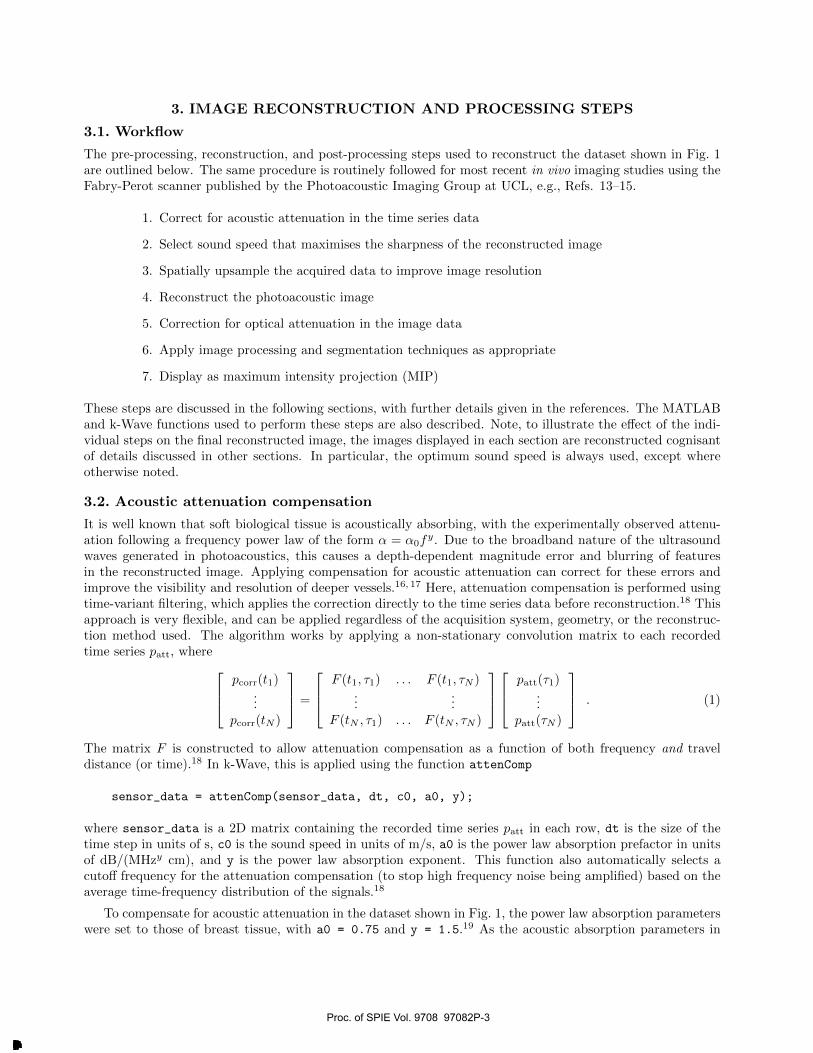
Figure 2. Three-dimensional reconstructions of the dataset shown in Fig. 1 with and without attenuation compensation.The three vertical panels show maximum intensity projections (MIPs) through the depth and lateral directions, anda one-dimensional profile through the lateral MIP at the location shown with a dashed white line. Magnification ofthe depth MIPs within the square dotted boxes is shown in the two right panels. Including attenuation compensationincreases the sharpness of the vasculature and tumour, and improves the visibility and resolution of deeper vessels(arrows) without increasing the noise floor (circled region).

murine tissue are not well characterised, the average value in breast tissue is an apposite choice for soft-tissuecontaining a range of tissue types. The noise threshold and energy threshold used to select the filter cutofffrequency were set to 5% and 95%, respectively. The average time frequency distribution and the automaticallyselected filter cutoff frequency are shown in Fig. 1(d). Reconstructed images with and without acoustic atten-uation compensation are shown in Fig. 2 for comparison. The tumour can be clearly seen as the sponge likestructure in the centre of the image, along with the surrounding blood vasculature. When attenuation com-pensation is included, the sharpness of the vasculature and tumour is increased. This is particularly noticeablein the magnified images, which show an improvement down to the voxel level. The visibility and resolution ofdeeper vessels is also improved, as shown in the one-dimensional profiles. For example, the visibility and sharp-ness of the vessel denoted with the black arrows has significantly increased, without a corresponding increasein the noise floor (circled region). It is useful to point out that these improvements are not an image processingtrick; they arise directly from rectifying the acoustic losses that physically occur as the photoacoustic wavespropagate through tissue.



Regarding computational time, acoustic attenuation compensation using time variant filtering is very fastto apply. Using a desktop PC with an 8-core Intel Xeon E5-1660 v3 @ 3 GHz processor running MATLAB2015a, the attenComp function took 3.1 s to calculate the average time frequency distribution, 0.45 s to selectthe cutoff frequency for the filter, 0.042 s to create the filter, and 0.19 s to apply the correction to all 20,022time domain waveforms. If the filter cutoff frequency is chosen manually (based on the noise floor in the powerspectrum for example20), there is no need to calculate the time frequency distribution, and the correction iseven faster to apply.

3.3. Sound speed selection

The reconstruction of photoacoustic images requires knowledge of the sound speed within the medium so time-of-flight measurements can be correctly mapped back to the initial pressure distribution. Most reconstructionalgorithms routinely used assume a constant value of sound speed. However, for in vivo imaging, the true valueof sound speed is usually unknown. It is possible to estimate an appropriate value by systematically modifyingthe sound speed until the sharpness of the reconstructed image is maximised.8, 21 This is based on the premisethat features in the imaging volume are inherently sharp, and thus the correct sound speed is the one thatproduces the sharpest looking image. In k-Wave, sharpness is evaluated using the function sharpness.21 Bydefault, this uses a sharpness metric or focus function based on a simple finite difference gradient calculationknown as the Brenner gradient. In 2D this is given by

Fbrenner =∑x,y

(fx+2,y − fx,y)2

+ (fx,y+2 − fx,y)2. (2)

The sound speed value that maximises the sharpness metric can then be found by looping through a range ofvalues as shown below, or using simple optimisation routines (e.g., fminbnd in MATLAB).

% set range of sound speeds to test

c_array = c_min:c_step:c_max;

% loop through sound speeds

for c_index = 1:length(c_array)

% compute reconstruction using current value of sound speed

recon = ...

% take maximum intensity projection along the depth direction

mip = max(recon, [], 3)

% compute sharpness metric

sharpness_metric(c_index) = sharpness(mip);

end

% find the index of the maximum sharpness

[~, max_index] = max(sharpness_metric);

% assign optimum sound speed

c_opt = c_array(max_index);

Figure 3(a) shows depth direction (enface) maximum intensity projections (MIPs) of the reconstructedtumour image using six different values of sound speed from 1400 m/s to 1600 m/s. As the sound speedis increased, the image is gradually focused and then defocused again. The corresponding focus functioncalculated using Eq. (2) is shown in Fig. 3(b). In this case, the focus function is unimodal, with a peak at1515 m/s (shown with the dashed line). This is within the range of physiological values between fat (1430



1400 m/s(a)

(b)

1450 m/s 1500 m/s

1550 m/s 1600 m/s 1515 m/s

1 mm

1400 1450 1500 1550 16000.4

0.6

0.8

1

Sound Speed [m/s]

No

rma

lise

d F

ocu

s F

un

ctio

n

x

y

Figure 3. (a) Depth direction maximum intensity projections of the reconstructed image using different values forsound speed. A focusing and then defocusing can be noticed as the sound speed is increased. The reconstructed imageusing the sound speed that maximises the focus function (sharpness metric) is shown in the bottom right panel. (b)Variation of the focus function for sound speed values between 1400 and 1600 m/s. The focus function is unimodal, andthe value of sound speed that maximises the focus function is shown with a dashed line. The steps used by fminbnd inMATLAB to find the maximum are shown with the grey dots.

m/s) and muscle (1580 m/s).19 The reconstructed image using the optimised value for sound speed is shown inthe bottom right panel of Fig. 3(a). The computational cost of computing the MIP and sharpness metric arenegligible, thus the main cost of this approach is the repeated image reconstruction that must be performed.Using fminbnd in MATLAB, the optimum value for sound speed is found in 6 steps, shown as the grey dotsin Fig. 3(b). Combined with an optimised C++ version of the FFT-based algorithm described in Sec. 3.5, thecomplete autofocusing procedure takes less than 5 seconds.

3.4. Upsampling

Due to practical constraints of using the Fabry-Perot scanning system (including animal scanning times andacquisition memory depth), the temporal sampling used for in vivo imaging studies is typically higher than



the spatial sampling (the same is true of most photoacoustic and ultrasound scanners). For the samplingparameters used for the tumour dataset, the maximum supported frequencies due to the temporal and spatialsampling are

fmax,t =1

2∆t= 25 MHz > fmax,x =

c

2∆x= 7.575 MHz . (3)

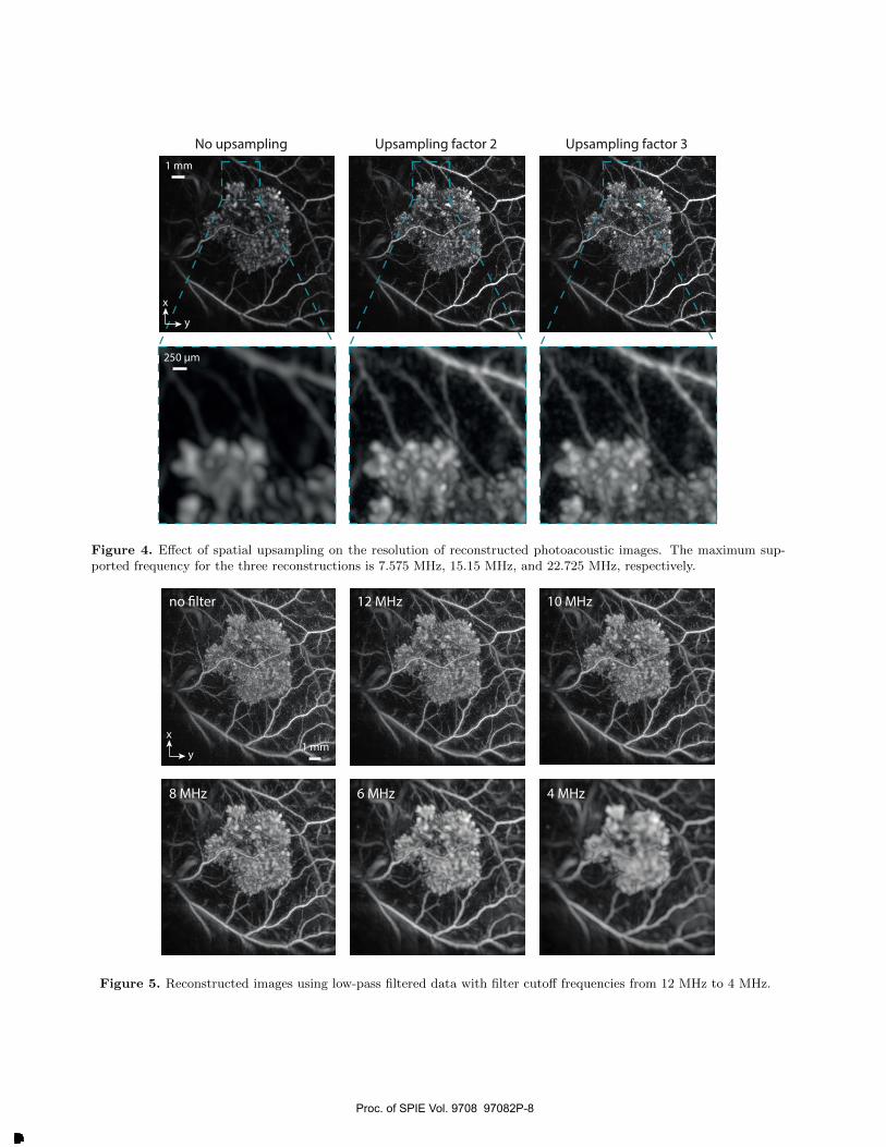
As shown in Fig. 1(c), the acquired photoacoustic signals are very broadband, containing energy up to∼20 MHz.This means the acquisition is spatially undersampled. Thus, if the image is reconstructed onto a grid definedby the spatial acquisition parameters, higher frequency information contained in the temporal signals will notbe used, reducing resolution. To overcome this, the grid parameters used for the reconstruction can be spatiallyupsampled. This is demonstrated in Fig. 4, where the tumour image has been reconstructed using time reversalwith upsampling factors of 1 (no upsampling), 2 and 3. This corresponds to a grid spacing (and maximumsupported frequency) of 100 µm (7.575 MHz), 50 µm (15.15 MHz), and 33 µm (22.725 MHz), respectively. Toallow a fair comparison, all three reconstructed images have been resampled to the same resolution for displayusing Fourier interpolation (interpftn in k-Wave). There is a very clear improvement with an upsamplingfactor of 2 compared to no upsampling. The small vessels are more visible, and there is much greater detailin the tumour mass. In comparison, there is little perceptible different between the reconstructed images with2 and 3 times upsampling, despite the latter allowing almost the full range of frequencies contained in thetemporal signals to be used in the reconstruction.

To examine this in more detail, the tumour dataset was reconstructed with an upsampling factor of 3 afterfirst low-pass filtering the time signals. The reconstructed images for filter cutoff frequencies between 12 MHzand 4 MHz are shown in Fig. 5. For filter cutoff frequencies above 12 MHz, there was no discernible changein the image. At 12 MHz, the magnitude of the reconstructed image starts to decrease, and there is a slightreduction in high frequency variations at the voxel level. At 10 MHz, the main features are all still discernible,but begin to become noticeably softer. This trend continues down to 4 MHz, where the tumour and mainvessels are still visible, but significantly blurred. Thus for this dataset, qualitatively it would appear that thefrequency content up to ∼12 MHz has a perceptible impact on the reconstructed image. This explains whythere is no noticeable difference seen between upsampling factors of 2 and 3 shown in Fig. 4.

The computational cost of using upsampling (particularly with time reversal image reconstruction) is thatthe image reconstruction must be performed using a larger computational grid. The grid size, compute time,and memory usage for the three reconstructions shown in Fig. 4 (using the 20,022 recorded time series) aregiven in Table 1. The reconstructions were performed using an optimised C++/CUDA version of k-Waverunning on an NVIDIA GeForce GTX TITAN X graphics processing unit (GPU).22 Even at the largest scale,the reconstruction takes less than 30 seconds and uses less than 4 GB of memory.

Table 1. Summary of grid size and compute time to reconstruct the tumour image using time reversal with differentupsampling factors.

Upsampling Factor Grid Size Compute Time Memory Usage

1 162 × 162 × 96 1.5 s 419 MB2 324 × 324 × 144 8.1 s 1320 MB3 450 × 450 × 216 25.3 s 3368 MB

3.5. Reconstruction methods

Two algorithms are routinely used for reconstructing the datasets acquired using the planar Fabry-Perot scan-ning system. The first is a fast one-step method based on an interpolation between spatial and temporalfrequency performed in the Fourier domain as shown below (kspacePlaneRecon in k-Wave).23, 24

p(x, y, t)FFT−−−→ P (kx, ky, ω)

ωc2 =k2

x+k2y+k2

z−−−−−−−−−−→ H(kx, ky, kz)IFFT−−−→ h(x, y, z) (4)

The second is time reversal, where the detected signals are propagated back into the domain in time reversedorder using a numerical model of the acoustic forward problem (kspaceFirstOrder3D in k-Wave).17, 25, 26



Il th

No upsampling Upsampling factor 2 Upsampling factor 3

1 mm

250 μm

x

y

Figure 4. Effect of spatial upsampling on the resolution of reconstructed photoacoustic images. The maximum sup-ported frequency for the three reconstructions is 7.575 MHz, 15.15 MHz, and 22.725 MHz, respectively.

no �lter 12 MHz 10 MHz

8 MHz 6 MHz 4 MHz

1 mmx

y

Figure 5. Reconstructed images using low-pass filtered data with filter cutoff frequencies from 12 MHz to 4 MHz.



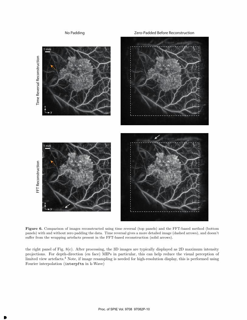
A comparison of the images produced by these two methods is shown in Fig. 6. Because of the differentassumptions inherent in the two algorithms, they produce visibly different images. First, the time reversalimage has noticeably more detail, particularly in the tumour mass and smaller vasculature (e.g., the vesseldenoted with the dashed arrows). This may be due to the way high-frequency information is mapped into theimage in time reversal, and the inclusion of evanescent waves in the reconstruction.10 Second, the FFT-basedimage contains wrapping artefacts due to the assumed spatial periodicity of the data. This is clearly visiblewhen the reconstruction is repeated after spatially zero-padding the time domain signals (right panels). Forexample, the vessel denoted with the solid arrow belongs at the top of the image outside the field of view(bottom right panel), but is mapped to the bottom of the FFT-based image without zero-padding (bottom leftpanel). The main advantage of the FFT-based algorithm is its speed. Consequently, it is used for the soundspeed optimisation step discussed in Sec. 3.3, and real-time display. Time reversal is generally used for all otherpurposes.

3.6. Image processing

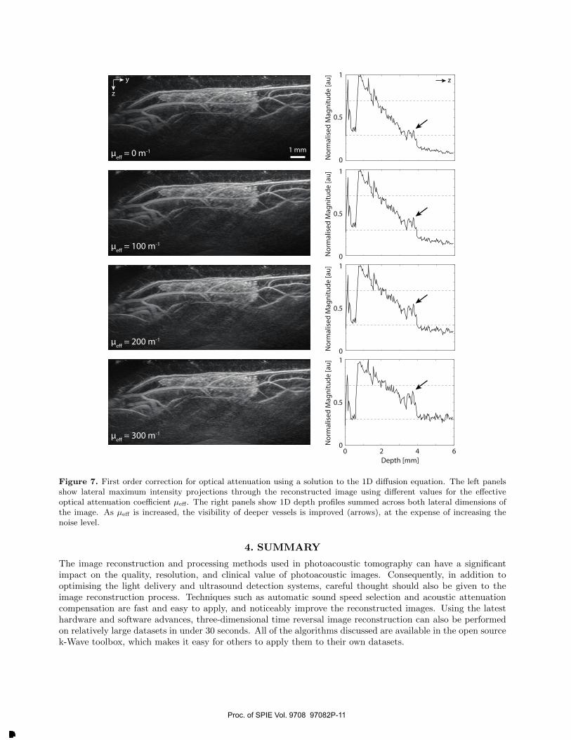
After reconstruction, very basic image processing is performed. First, a positivity condition is usually appliedwhere negative acoustic pressures in the reconstructed image are thresholded to zero.27 Next, to improve thevisibility of deeper lying vessels, a simple first-order correction for the variable light fluence in tissue is appliedusing a solution to the 1D diffusion equation

Φ(z) = Φ0 exp(−µeffz) . (5)

Here Φ(z) is the light fluence at depth z, and µeff is the effective attenuation coefficient, which can be in therange 50 − 250 m−1 depending on the type of tissue. Note, this assumes the optical illumination is a planarcollimated beam at the top surface of the tissue, the fluence is diffuse everywhere, and the optical properties areconstant throughout the tissue.7 These assumptions do not hold in general, thus this step does not quantitivelycorrect for the spatial distribution of the fluence, but rather, qualitatively improves the visibility of deeperstructures which in general will have received less light.

The effect of changing µeff on the lateral MIP of the tumour image is shown in Fig. 7. The right panelsshow 1D depth profiles summed across both lateral dimensions of the image, and give the total image intensityas a function of depth. If the image features were distributed evenly throughout the imaging volume, the peaksin the 1D profile would have approximately the same amplitude. However, because of optical attenuation, theimage intensity rapidly decays with depth. As µeff is increased, the visibility of deeper structures is improvedand the image intensity becomes more uniform. However, this comes at the expense of increasing the noiselevel, particularly at greater depths in the image.

In addition to correction for optical attenuation, the image data is often log compressed to reduce thedynamic range of the image before display (analogous to the log compression performed in ultrasound imaging).The log compression is performed according to

hcompressed =log10

(1 + 2l × h

)log10 (1 + 2l)

, (6)

where h is the image data normalised between 0 and 1, and l is the compression level, which is typicallyset between 0 (low compression) and 4 (high compression). In k-Wave, this is applied using the functionlogCompression. The nonlinear mapping given by Eq. (6) is plotted in Fig. 8(a), and the log compressedimages using l set to 1 and 4 are shown in Fig. 8(b). The compression makes it significantly easier to visualisethe different structures in the image, particularly the small vasculature.

No other image processing (e.g., denoising) is routinely applied to the reconstructed images. In some cases,a manual segmentation and false colour might be used to highlight different regions of the image as shown inthe left panel of Fig. 8(c). k-Wave also includes a vessel filtering function (vesselFilter), the output of whichis shown in the middle panel of Fig. 8(c).28 However, this is less useful in the case of the tumour image, whichappears almost cartoon like. Finally, in some cases a colour map is used for depth direction (en face) maximumintensity projections to illustrate the depth at which the maximum value is extracted. An example is shown in



x

y

1 mm

x

y

1 mm

FF

T R

eco

nst

ruct

ion

Tim

e R

ev

ers

al R

eco

nst

ruct

ion

No Padding Zero-Padded Before Reconstruction

Figure 6. Comparison of images reconstructed using time reversal (top panels) and the FFT-based method (bottompanels) with and without zero padding the data. Time reversal gives a more detailed image (dashed arrows), and doesn’tsuffer from the wrapping artefacts present in the FFT-based reconstruction (solid arrows).

the right panel of Fig. 8(c). After processing, the 3D images are typically displayed as 2D maximum intensityprojections. For depth-direction (en face) MIPs in particular, this can help reduce the visual perception oflimited view artefacts.4 Note, if image resampling is needed for high-resolution display, this is performed usingFourier interpolation (interpftn in k-Wave)



z

y z

1 mmμe"

= 0 m-1

μe"

= 100 m-1

μe"

= 200 m-1

μe"

= 300 m-1

0 2 4 6

Depth [mm]

0

0.5

1

No

rma

lise

d M

ag

nit

ud

e [

au

]

0

0.5

1

No

rma

lise

d M

ag

nit

ud

e [

au

]

0

0.5

1

No

rma

lise

d M

ag

nit

ud

e [

au

]

0

0.5

1

No

rma

lise

d M

ag

nit

ud

e [

au

]

Figure 7. First order correction for optical attenuation using a solution to the 1D diffusion equation. The left panelsshow lateral maximum intensity projections through the reconstructed image using different values for the effectiveoptical attenuation coefficient µeff. The right panels show 1D depth profiles summed across both lateral dimensions ofthe image. As µeff is increased, the visibility of deeper vessels is improved (arrows), at the expense of increasing thenoise level.

4. SUMMARY

The image reconstruction and processing methods used in photoacoustic tomography can have a significantimpact on the quality, resolution, and clinical value of photoacoustic images. Consequently, in addition tooptimising the light delivery and ultrasound detection systems, careful thought should also be given to theimage reconstruction process. Techniques such as automatic sound speed selection and acoustic attenuationcompensation are fast and easy to apply, and noticeably improve the reconstructed images. Using the latesthardware and software advances, three-dimensional time reversal image reconstruction can also be performedon relatively large datasets in under 30 seconds. All of the algorithms discussed are available in the open sourcek-Wave toolbox, which makes it easy for others to apply them to their own datasets.



-'911C:

1

(b)

(a)

(c)

1 mm

no compression l = 1 l = 4

false colour vessel !lter depth to colour

[mm

]

5

4

3

2

1

0

x

y

Input value

0 0.5 1

Ou

tpu

t v

alu

e

0

0.5

1

No compression

l = 0 (lowest)

l = 1 (low)

l = 2 (medium)

l = 3 (high)

l = 4 (highest)

Figure 8. (a) Log compression curves for compression values from 0 to 4 calculated using Eq. (6). (b) Reconstructedphotoacoustic images with no compression (left panel), log compression with l = 1 (middle panel), and log compressionwith l = 4 (right panel). (c) Other image processing techniques include false colour (left panel), vessel filtering (middlepanel), and depth colour coded maximum intensity projections (right panel).

ACKNOWLEDGMENTS

The authors would like to thank Prof. Paul Beard, head of the Photoacoustic Imaging Group, for his contribu-tion to the algorithms described in this paper, and valuable comments on the manuscript. This work was sup-ported by the Engineering and Physical Sciences Research Council, UK (EP/L020262/1 and EP/M011119/1).The experimental data used in this study was provided by Amit Jathoul, Jan Laufer, Olumide Ogunlade,Bradley Treeby, Ben Cox, Edward Zhang, Peter Johnson, Arnold Pizzey, Brian Philip, Teresa Marafioti, MarkLythgoe, R Barbara Pedley, Martin Pule, and Paul Beard. See Ref. 11 for details. Jiri Jaros is financed fromthe SoMoPro II Programme, co-financed by the European Union and the South-Moravian Region. This workreflects only the author’s view and the European Union is not liable for any use that may be made of theinformation contained therein.



REFERENCES

1. P. Beard, “Biomedical photoacoustic imaging,” Interface Focus 1(4), pp. 602–631, 2011.

2. M. Lakshman and A. Needles, “Screening and quantification of the tumor microenvironment with micro-ultrasound and photoacoustic imaging,” Nat. Meth. 12(4), pp. iii–v, 2015.

3. P. Kuchment and L. Kunyansky, “Mathematics of Photoacoustic and Thermoacoustic Tomography,” inHandbook of Mathematical Methods in Imaging, ch. 19, pp. 817–865, Springer, 2011.

4. Y. Xu, L. V. Wang, G. Ambartsoumian, and P. Kuchment, “Reconstructions in limited-view thermoa-coustic tomography,” Med. Phys. 31(4), pp. 724–733, 2004.

5. B. T. Cox and B. E. Treeby, “Effect of sensor directionality on photoacoustic imaging: A study using thek-Wave toolbox,” in Proc. of SPIE, 7564, pp. 6–11, 2010.

6. N. A. Rejesh, H. Pullagurla, and M. Pramanik, “Deconvolution-based deblurring of reconstructed imagesin photoacoustic/thermoacoustic tomography,” J. Opt. Soc. Am. A 30(10), pp. 1994–2001, 2013.

7. B. Cox, J. G. Laufer, S. R. Arridge, and P. C. Beard, “Quantitative spectroscopic photoacoustic imaging:A review,” J. Biomed. Opt. 17(6), p. 061202, 2012.

8. C. Yoon, J. Kang, S. Han, Y. Yoo, T.-K. Song, and J. H. Chang, “Enhancement of photoacoustic imagequality by sound speed correction: Ex vivo evaluation,” Opt. Express 20(3), pp. 3082–3090, 2012.

9. D. Van de Sompel, L. S. Sasportas, A. Dragulescu-Andrasi, S. Bohndiek, and S. S. Gambhir, “Improvingimage quality by accounting for changes in water temperature during a photoacoustic tomography scan,”PloS one 7(10), p. e45337, 2012.

10. B. E. Treeby and B. T. Cox, “k-Wave: MATLAB toolbox for the simulation and reconstruction of pho-toacoustic wave fields,” J. Biomed. Opt. 15(2), p. 021314, 2010.

11. A. P. Jathoul, J. Laufer, O. Ogunlade, B. Treeby, B. Cox, E. Zhang, P. Johnson, A. R. Pizzey, B. Philip,T. Marafioti, M. F. Lythgoe, R. B. Pedley, M. A. Pule, and P. Beard, “Deep in vivo photoacoustic imagingof mammalian tissues using a tyrosinase-based genetic reporter,” Nat. Photon. 9, pp. 239–246, 2015.

12. E. Zhang, J. Laufer, and P. Beard, “Backward-mode multiwavelength photoacoustic scanner using a planarFabry-Perot polymer film ultrasound sensor for high-resolution three-dimensional imaging of biologicaltissues,” Appl. Optics 47(4), pp. 561–577, 2008.

13. J. Laufer, P. Johnson, E. Zhang, B. Treeby, B. Cox, B. Pedley, and P. Beard, “In vivo preclinical pho-toacoustic imaging of tumor vasculature development and therapy,” J. Biomed. Opt. 17(5), p. 056016,2012.

14. J. Laufer, F. Norris, J. Cleary, E. Zhang, B. Treeby, B. Cox, P. Johnson, P. Scambler, M. Lythgoe, andP. Beard, “In vivo photoacoustic imaging of mouse embryos,” J. Biomed. Opt. 17(6), p. 061220, 2012.

15. S. P. Johnson, O. Ogunlade, E. Zhang, J. Laufer, V. Rajkumar, R. B. Pedley, and P. Beard, “Photoacoustictomography of vascular therapy in a preclinical mouse model of colorectal carcinoma,” in Proc. of SPIE,8943, p. 89431R, 2014.

16. P. Burgholzer, H. Grun, M. Haltmeier, R. Nuster, and G. Paltauf, “Compensation of acoustic attenuationfor high resolution photoacoustic imaging with line detectors,” in Proc. of SPIE, 6437, p. 643724, 2007.

17. B. E. Treeby, E. Z. Zhang, and B. T. Cox, “Photoacoustic tomography in absorbing acoustic media usingtime reversal,” Inverse Probl. 26(11), p. 115003, 2010.

18. B. E. Treeby, “Acoustic attenuation compensation in photoacoustic tomography using time-variant filter-ing,” J. Biomed. Opt. 18(3), p. 036008, 2013.

19. T. L. Szabo, Diagnostic Ultrasound Imaging, Elsevier Academic Press, London, 2004.

20. B. E. Treeby, J. G. Laufer, E. Z. Zhang, F. C. Norris, M. F. Lythgoe, P. C. Beard, and B. T. Cox,“Acoustic attenuation compensation in photoacoustic tomography: Application to high-resolution 3Dimaging of vascular networks in mice,” in Proc. of SPIE, 7899, p. 78992Y, 2011.

21. B. E. Treeby, T. K. Varslot, E. Z. Zhang, J. G. Laufer, and P. C. Beard, “Automatic sound speed selectionin photoacoustic image reconstruction using an autofocus approach,” J. Biomed. Opt. 16(9), p. 090501,2011.

22. B. E. Treeby, J. Jaros, A. P. Rendell, and B. T. Cox, “Modeling nonlinear ultrasound propagation inheterogeneous media with power law absorption using a k-space pseudospectral method,” J. Acoust. Soc.Am. 131(6), pp. 4324–4336, 2012.



23. S. J. Norton and M. Linzer, “Ultrasonic reflectivity imaging in three dimensions: Exact inverse scatteringsolutions for plane, cylindrical, and spherical apertures,” IEEE T. Biomed. Eng. 28(2), pp. 202–220, 1981.

24. K. P. Koestli, M. Frenz, H. Bebie, H. P. Weber, K. P. Kostli, M. Frenz, H. Bebie, and H. P. Weber,“Temporal backward projection of optoacoustic pressure transients using Fourier transform methods,”Phys. Med. Biol. 46(7), pp. 1863–1872, 2001.

25. D. Finch, S. K. Patch, and Rakesh, “Determining a function from its mean values over a family of spheres,”SIAM J. Math. Anal. 35(5), pp. 1213–1240, 2004.

26. Y. Xu and L. Wang, “Time reversal and its application to tomography with diffracting sources,” Phys.Rev. Lett. 92(3), pp. 3–6, 2004.

27. G. Paltauf, J. A. Viator, S. A. Prahl, and S. L. Jacques, “Iterative reconstruction algorithm for optoacousticimaging,” J. Acoust. Soc. Am. 112(4), p. 1536, 2002.

28. T. Oruganti, J. Laufer, and B. E. Treeby, “Vessel filtering of photoacoustic images,” in Proc. of SPIE,8581, p. 85811W, 2013.



Documents

Advanced photoacoustic image reconstruction using the · PDF fileAdvanced photoacoustic image reconstruction using the ... Super cially, this would ... All of the algorithms discussed