Embed Size (px)
Citation preview
Feature Reconstruction in Tomography
Feature Reconstruction in Tomography
Alfred K. Louis
Institut für Angewandte MathematikUniversität des Saarlandes
66041 Saarbrückenhttp://www.num.uni-sb.de
Wien, July 20, 2009
Feature Reconstruction in Tomography
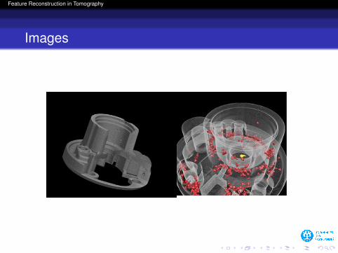
Images
Feature Reconstruction in Tomography
Typical Procedure
Image ReconstructionImage EnhancementDisadvantage: The two operations are non adjusted andpossibly too time-consuming
Feature Reconstruction in Tomography
Typical Procedure
Image Reconstruction
Image EnhancementDisadvantage: The two operations are non adjusted andpossibly too time-consuming
Feature Reconstruction in Tomography
Typical Procedure
Image ReconstructionImage Enhancement
Disadvantage: The two operations are non adjusted andpossibly too time-consuming
Feature Reconstruction in Tomography
Typical Procedure
Image ReconstructionImage EnhancementDisadvantage: The two operations are non adjusted andpossibly too time-consuming
Feature Reconstruction in Tomography
Requirements for Repeated Solution of SameProblem with Different Data
Combination of reconstruction and image analysis in ONEstepPrecompute solution operator for efficient evaluation of thesame problem with different data setsUse properties of the operator for fast algorithms
Feature Reconstruction in Tomography
Requirements for Repeated Solution of SameProblem with Different Data
Combination of reconstruction and image analysis in ONEstep
Precompute solution operator for efficient evaluation of thesame problem with different data setsUse properties of the operator for fast algorithms
Feature Reconstruction in Tomography
Requirements for Repeated Solution of SameProblem with Different Data
Combination of reconstruction and image analysis in ONEstepPrecompute solution operator for efficient evaluation of thesame problem with different data sets
Use properties of the operator for fast algorithms
Feature Reconstruction in Tomography
Requirements for Repeated Solution of SameProblem with Different Data
Combination of reconstruction and image analysis in ONEstepPrecompute solution operator for efficient evaluation of thesame problem with different data setsUse properties of the operator for fast algorithms
Feature Reconstruction in Tomography
Content
1 Formulation of Problem
2 Inverse Problems and Regularization
3 Approximate Inverse for Combining Reconstruction andAnalysis
4 Radon Transform and Edge Detection
5 Radon Transform and Diffusion
6 Radon Transform and Wavelet Decomposition
7 Nonlinear Problems
8 Future
Feature Reconstruction in Tomography
Formulation of Problem
Target
Combine the two steps in ONE algorithmInstead of
Solve reconstruction part Af = gEvaluate the result Lf
Compute directlyLA†g
Feature Reconstruction in Tomography
Formulation of Problem
Feature Determination
Image EnhancementImage RegistrationClassification
Feature Reconstruction in Tomography
Formulation of Problem
Examples of Existing Methods
A = R, L = I−1
Lambda CT 2D : Smith, VainbergLambda 3D: L-Maass, KatsevichLambda with SPECT, ET: Quinto, ÖktemLambda with SONAR : L., Quinto
Feature Reconstruction in Tomography
Formulation of Problem
Image Analysis
compute enhanced image Lfoperate on Lf
Example for Calculation
Lkβf =∂
∂xk
(Gβ ∗ f
)Edge Detection
L. 96: Compute directly derivative of solutionSchuster, 2000 : Compute divergence of vector fields
Feature Reconstruction in Tomography
Formulation of Problem
Image Analysis
compute enhanced image Lfoperate on Lf
Example for Calculation
Lkβf =∂
∂xk
(Gβ ∗ f
)Edge Detection
L. 96: Compute directly derivative of solutionSchuster, 2000 : Compute divergence of vector fields
Feature Reconstruction in Tomography
Formulation of Problem
Image Analysis
compute enhanced image Lfoperate on Lf
Example for Calculation
Lkβf =∂
∂xk
(Gβ ∗ f
)Edge Detection
L. 96: Compute directly derivative of solutionSchuster, 2000 : Compute divergence of vector fields
Feature Reconstruction in Tomography
Formulation of Problem
Applications for X-Ray CT
Detect defects like blowholesIn-line inspection3D Dimensioning ( dimensionelles Messen )
Feature Reconstruction in Tomography
Formulation of Problem
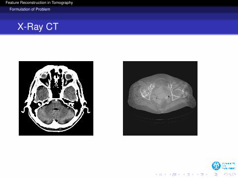
X-Ray CT
Feature Reconstruction in Tomography
Formulation of Problem
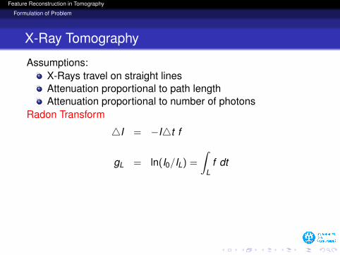
X-Ray Tomography
Assumptions:X-Rays travel on straight linesAttenuation proportional to path lengthAttenuation proportional to number of photons
Radon Transform
4I = −I4t f
gL = ln(I0/IL) =
∫L
f dt
Feature Reconstruction in Tomography
Formulation of Problem
X-Ray Tomography
Assumptions:X-Rays travel on straight linesAttenuation proportional to path lengthAttenuation proportional to number of photons
Radon Transform
4I = −I4t f
gL = ln(I0/IL) =
∫L
f dt
Feature Reconstruction in Tomography
Inverse Problems
Content
1 Formulation of Problem
2 Inverse Problems and Regularization
3 Approximate Inverse for Combining Reconstruction andAnalysis
4 Radon Transform and Edge Detection
5 Radon Transform and Diffusion
6 Radon Transform and Wavelet Decomposition
7 Nonlinear Problems
8 Future
Feature Reconstruction in Tomography
Inverse Problems
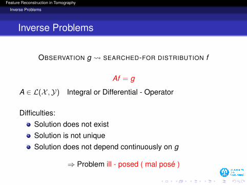
Inverse Problems
OBSERVATION g SEARCHED-FOR DISTRIBUTION f
Af = g
A ∈ L(X ,Y) Integral or Differential - Operator
Difficulties:Solution does not existSolution is not uniqueSolution does not depend continuously on g
⇒ Problem ill - posed ( mal posé )
Feature Reconstruction in Tomography
Inverse Problems
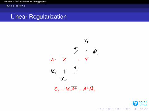
Linear Regularization
Y1
A+
↑ Mγ
A : X −→ Y
Mγ ↑A+
X−1
Sγ = MγA+ = A+Mγ
Feature Reconstruction in Tomography
Inverse Problems
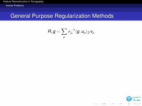
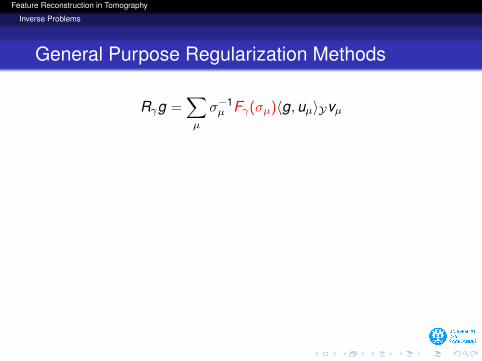
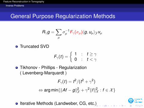
General Purpose Regularization Methods
Rγg =∑µ
σ−1µ 〈g,uµ〉Yvµ
Truncated SVD
Fγ(t) =
1 : t ≥ γ0 : t < γ
Tikhonov - Phillips - Regularization( Levenberg-Marquardt )
Fγ(t) = t2/(t2 + γ2)
⇔ arg min‖Af − g‖2Y + γ2‖f‖2X : f ∈ X
Iterative Methods (Landweber, CG, etc.)
Feature Reconstruction in Tomography
Inverse Problems
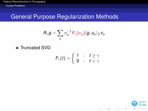
General Purpose Regularization Methods
Rγg =∑µ
σ−1µ Fγ(σµ)〈g,uµ〉Yvµ
Truncated SVD
Fγ(t) =
1 : t ≥ γ0 : t < γ
Tikhonov - Phillips - Regularization( Levenberg-Marquardt )
Fγ(t) = t2/(t2 + γ2)
⇔ arg min‖Af − g‖2Y + γ2‖f‖2X : f ∈ X
Iterative Methods (Landweber, CG, etc.)
Feature Reconstruction in Tomography
Inverse Problems
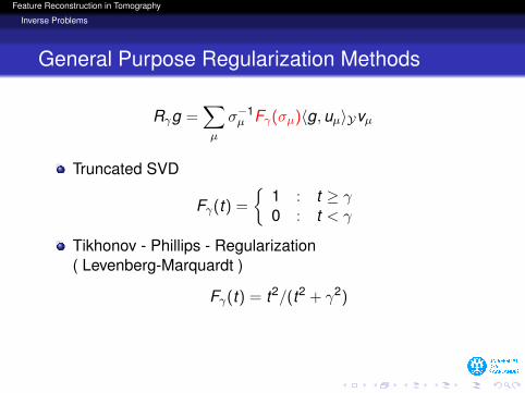
General Purpose Regularization Methods
Rγg =∑µ
σ−1µ Fγ(σµ)〈g,uµ〉Yvµ
Truncated SVD
Fγ(t) =
1 : t ≥ γ0 : t < γ
Tikhonov - Phillips - Regularization( Levenberg-Marquardt )
Fγ(t) = t2/(t2 + γ2)
⇔ arg min‖Af − g‖2Y + γ2‖f‖2X : f ∈ X
Iterative Methods (Landweber, CG, etc.)
Feature Reconstruction in Tomography
Inverse Problems
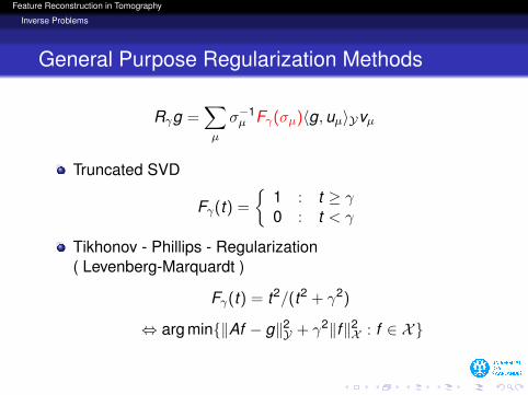
General Purpose Regularization Methods
Rγg =∑µ
σ−1µ Fγ(σµ)〈g,uµ〉Yvµ
Truncated SVD
Fγ(t) =
1 : t ≥ γ0 : t < γ
Tikhonov - Phillips - Regularization( Levenberg-Marquardt )
Fγ(t) = t2/(t2 + γ2)
⇔ arg min‖Af − g‖2Y + γ2‖f‖2X : f ∈ X
Iterative Methods (Landweber, CG, etc.)
Feature Reconstruction in Tomography
Inverse Problems
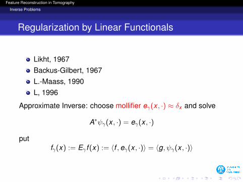
Regularization by Linear Functionals
Likht, 1967Backus-Gilbert, 1967L.-Maass, 1990L, 1996
Approximate Inverse: choose mollifier eγ(x , ·) ≈ δx and solve
A∗ψγ(x , ·) = eγ(x , ·)
putfγ(x) := Eγ f (x) := 〈f ,eγ(x , ·)〉 = 〈g, ψγ(x , ·)〉
Feature Reconstruction in Tomography
Inverse Problems
Regularization by Linear Functionals
Likht, 1967Backus-Gilbert, 1967L.-Maass, 1990L, 1996
Approximate Inverse: choose mollifier eγ(x , ·) ≈ δx and solve
A∗ψγ(x , ·) = eγ(x , ·)
putfγ(x) := Eγ f (x) := 〈f ,eγ(x , ·)〉 = 〈g, ψγ(x , ·)〉
Feature Reconstruction in Tomography
Approximate Inverse for Combining Reconstruction and Analysis
Content
1 Formulation of Problem
2 Inverse Problems and Regularization
3 Approximate Inverse for Combining Reconstruction andAnalysis
4 Radon Transform and Edge Detection
5 Radon Transform and Diffusion
6 Radon Transform and Wavelet Decomposition
7 Nonlinear Problems
8 Future
Feature Reconstruction in Tomography
Approximate Inverse for Combining Reconstruction and Analysis
Approximate Inverse
L.: SIAM J. Imaging Sciences 1 188-208, 2008
Aim Solve Af = g and compute Lf in one step
Smoothed version (Lf )γ = 〈Lf ,eγ〉 with mollifier eγ
Assume a solution exists of
A∗ψγ(x , ·) = L∗eγ(x , ·)
Then(Lf )γ(x) = 〈g, ψγ(x , ·)〉
Feature Reconstruction in Tomography
Approximate Inverse for Combining Reconstruction and Analysis
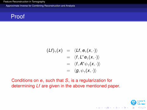
Proof
(Lf )γ(x) = 〈Lf ,eγ(x , ·)〉= 〈f ,L∗eγ(x , ·)〉= 〈f ,A∗ψγ(x , ·)〉= 〈g, ψγ(x , ·)〉
Conditions on eγ such that Sγ is a regularization fordetermining Lf are given in the above mentioned paper.
Feature Reconstruction in Tomography
Approximate Inverse for Combining Reconstruction and Analysis
Proof
(Lf )γ(x) = 〈Lf ,eγ(x , ·)〉= 〈f ,L∗eγ(x , ·)〉= 〈f ,A∗ψγ(x , ·)〉= 〈g, ψγ(x , ·)〉
Conditions on eγ such that Sγ is a regularization fordetermining Lf are given in the above mentioned paper.
Feature Reconstruction in Tomography
Approximate Inverse for Combining Reconstruction and Analysis
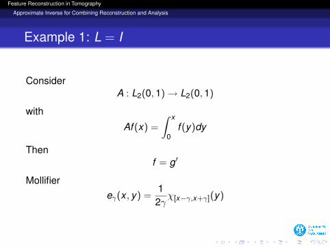
Example 1: L = I
ConsiderA : L2(0,1)→ L2(0,1)
with
Af (x) =
∫ x
0f (y)dy
Thenf = g′
Mollifiereγ(x , y) =
12γχ[x−γ,x+γ](y)
Feature Reconstruction in Tomography
Approximate Inverse for Combining Reconstruction and Analysis
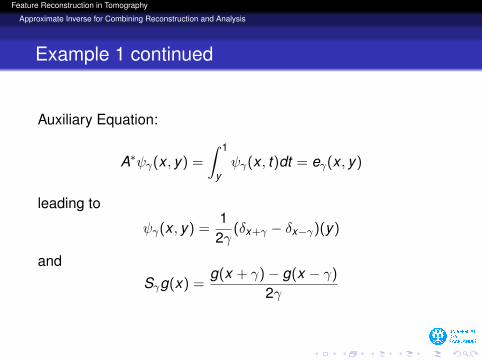
Example 1 continued
Auxiliary Equation:
A∗ψγ(x , y) =
∫ 1
yψγ(x , t)dt = eγ(x , y)
leading to
ψγ(x , y) =1
2γ(δx+γ − δx−γ)(y)
andSγg(x) =
g(x + γ)− g(x − γ)
2γ
Feature Reconstruction in Tomography
Approximate Inverse for Combining Reconstruction and Analysis
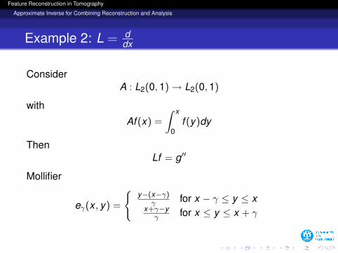
Example 2: L = ddx
ConsiderA : L2(0,1)→ L2(0,1)
with
Af (x) =
∫ x
0f (y)dy
ThenLf = g′′
Mollifier
eγ(x , y) =
y−(x−γ)
γ for x − γ ≤ y ≤ xx+γ−y
γ for x ≤ y ≤ x + γ
Feature Reconstruction in Tomography
Approximate Inverse for Combining Reconstruction and Analysis
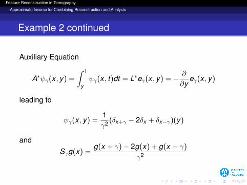
Example 2 continued
Auxiliary Equation
A∗ψγ(x , y) =
∫ 1
yψγ(x , t)dt = L∗eγ(x , y) = − ∂
∂yeγ(x , y)
leading to
ψγ(x , y) =1γ2 (δx+γ − 2δx + δx−γ)(y)
andSγg(x) =
g(x + γ)− 2g(x) + g(x − γ)
γ2
Feature Reconstruction in Tomography
Approximate Inverse for Combining Reconstruction and Analysis
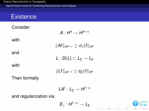
Existence
ConsiderA : Hs → Hs+α
with‖Af‖Hs+α ≥ c1‖f‖Hs
andL : D(L) ⊂ L2 → L2
with‖Lf‖Hs−t ≤ c2‖f‖Hs
Then formally
LA† : L2 → H t−α
and regularization via
Eγ : H t−α → L2
Feature Reconstruction in Tomography
Approximate Inverse for Combining Reconstruction and Analysis
Possibilities
t < 0: addtional regularization needed( Ex.: L differentiation )t = 0: only regularization of A needed( Ex.: Wavelet decomposition )t > α: no regularization at all( Ex.: diffusion )
Feature Reconstruction in Tomography
Approximate Inverse for Combining Reconstruction and Analysis
Possibilities
t < 0: addtional regularization needed( Ex.: L differentiation )
t = 0: only regularization of A needed( Ex.: Wavelet decomposition )t > α: no regularization at all( Ex.: diffusion )
Feature Reconstruction in Tomography
Approximate Inverse for Combining Reconstruction and Analysis
Possibilities
t < 0: addtional regularization needed( Ex.: L differentiation )t = 0: only regularization of A needed( Ex.: Wavelet decomposition )
t > α: no regularization at all( Ex.: diffusion )
Feature Reconstruction in Tomography
Approximate Inverse for Combining Reconstruction and Analysis
Possibilities
t < 0: addtional regularization needed( Ex.: L differentiation )t = 0: only regularization of A needed( Ex.: Wavelet decomposition )t > α: no regularization at all( Ex.: diffusion )
Feature Reconstruction in Tomography
Approximate Inverse for Combining Reconstruction and Analysis
Invariances
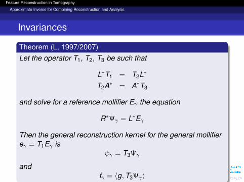
Theorem (L, 1997/2007)Let the operator T1, T2, T3 be such that
L∗T1 = T2L∗
T2A∗ = A∗T3
and solve for a reference mollifier Eγ the equation
R∗Ψγ = L∗Eγ
Then the general reconstruction kernel for the general mollifiereγ = T1Eγ is
ψγ = T3Ψγ
andfγ = 〈g,T3Ψγ〉
Feature Reconstruction in Tomography
Approximate Inverse for Combining Reconstruction and Analysis
Possible Calculation of Reconstruction Kernel
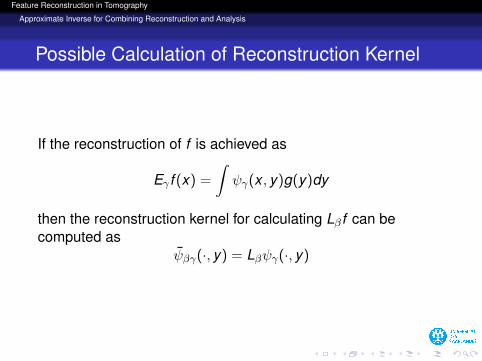
If the reconstruction of f is achieved as
Eγ f (x) =
∫ψγ(x , y)g(y)dy
then the reconstruction kernel for calculating Lβf can becomputed as
ψβγ(·, y) = Lβψγ(·, y)
Feature Reconstruction in Tomography
Radon Transform and Edge Detection
Content
1 Formulation of Problem
2 Inverse Problems and Regularization
3 Approximate Inverse for Combining Reconstruction andAnalysis
4 Radon Transform and Edge Detection
5 Radon Transform and Diffusion
6 Radon Transform and Wavelet Decomposition
7 Nonlinear Problems
8 Future
Feature Reconstruction in Tomography
Radon Transform and Edge Detection
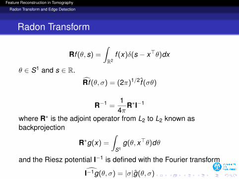
Radon Transform
Rf (θ, s) =
∫R2
f (x)δ(s − x>θ)dx
θ ∈ S1 and s ∈ R.
Rf (θ, σ) = (2π)1/2 f (σθ)
R−1 =1
4πR∗I−1
where R∗ is the adjoint operator from L2 to L2 known asbackprojection
R∗g(x) =
∫S1
g(θ, x>θ)dθ
and the Riesz potential I−1 is defined with the Fourier transformI−1g(θ, σ) = |σ|g(θ, σ)
Feature Reconstruction in Tomography
Radon Transform and Edge Detection
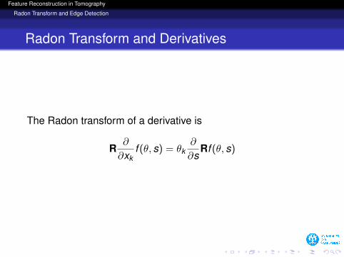
Radon Transform and Derivatives
The Radon transform of a derivative is
R∂
∂xkf (θ, s) = θk
∂
∂sRf (θ, s)
Feature Reconstruction in Tomography
Radon Transform and Edge Detection
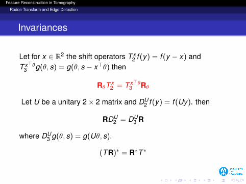
Invariances
Let for x ∈ R2 the shift operators T x2 f (y) = f (y − x) and
T x>θ3 g(θ, s) = g(θ, s − x>θ) then
RθT x2 = T x>θ
3 Rθ
Let U be a unitary 2× 2 matrix and DU2 f (y) = f (Uy). then
RDU2 = DU
3 R
where DU3 g(θ, s) = g(Uθ, s).
(T R)∗ = R∗T ∗
Feature Reconstruction in Tomography
Radon Transform and Edge Detection
Reconstruction Kernel
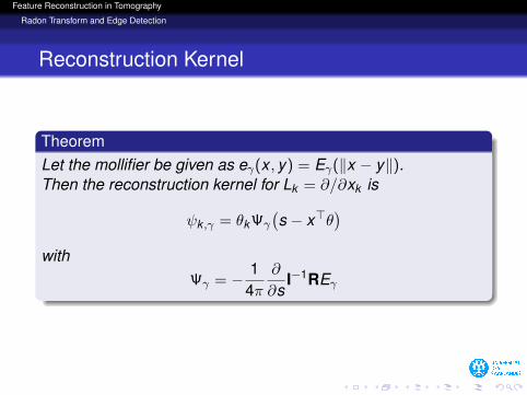
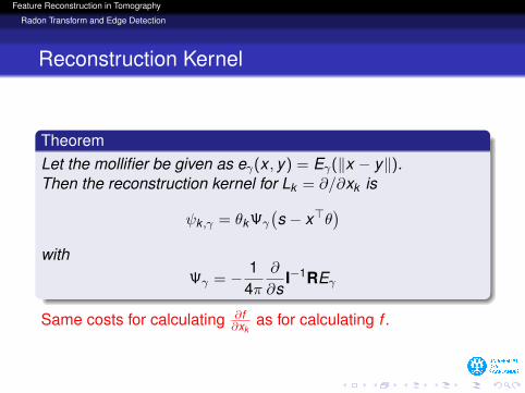
TheoremLet the mollifier be given as eγ(x , y) = Eγ(‖x − y‖).Then the reconstruction kernel for Lk = ∂/∂xk is
ψk ,γ = θk Ψγ
(s − x>θ
)with
Ψγ = − 14π
∂
∂sI−1REγ
Same costs for calculating ∂f∂xk
as for calculating f .
Feature Reconstruction in Tomography
Radon Transform and Edge Detection
Reconstruction Kernel
TheoremLet the mollifier be given as eγ(x , y) = Eγ(‖x − y‖).Then the reconstruction kernel for Lk = ∂/∂xk is
ψk ,γ = θk Ψγ
(s − x>θ
)with
Ψγ = − 14π
∂
∂sI−1REγ
Same costs for calculating ∂f∂xk
as for calculating f .
Feature Reconstruction in Tomography
Radon Transform and Edge Detection
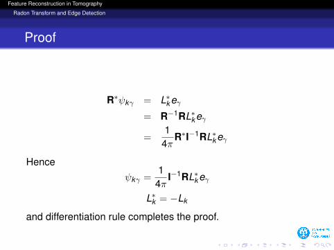
Proof
R∗ψkγ = L∗keγ= R−1RL∗keγ
=1
4πR∗I−1RL∗keγ
Henceψkγ =
14π
I−1RL∗keγ
L∗k = −Lk
and differentiation rule completes the proof.
Feature Reconstruction in Tomography
Radon Transform and Edge Detection
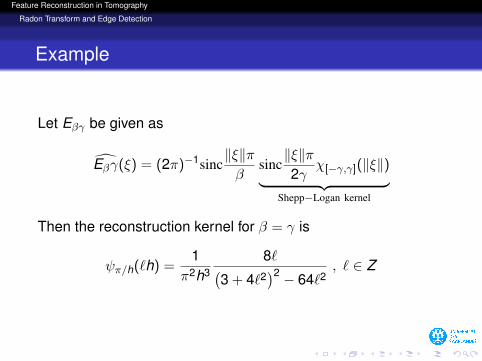
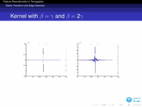
Example
Let Eβγ be given as
Eβγ(ξ) = (2π)−1sinc‖ξ‖πβ
sinc‖ξ‖π2γ
χ[−γ,γ](‖ξ‖)︸ ︷︷ ︸Shepp−Logan kernel
Then the reconstruction kernel for β = γ is
ψπ/h(`h) =1
π2h38`(
3 + 4`2)2 − 64`2
, ` ∈ Z
Feature Reconstruction in Tomography
Radon Transform and Edge Detection
Kernel with β = γ and β = 2γ
Feature Reconstruction in Tomography
Radon Transform and Edge Detection
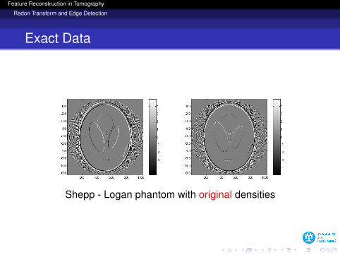
Exact Data
Shepp - Logan phantom with original densities
Feature Reconstruction in Tomography
Radon Transform and Edge Detection
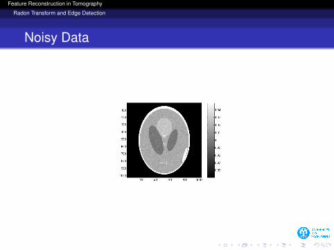
Noisy Data
Feature Reconstruction in Tomography
Radon Transform and Edge Detection
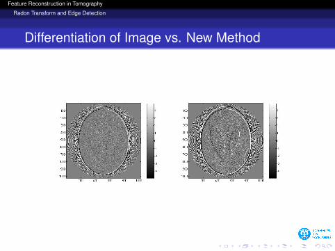
Differentiation of Image vs. New Method
Feature Reconstruction in Tomography
Radon Transform and Edge Detection
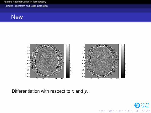
New
Differentiation with respect to x and y .
Feature Reconstruction in Tomography
Radon Transform and Edge Detection
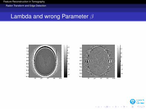
Lambda and wrong Parameter β
Feature Reconstruction in Tomography
Radon Transform and Edge Detection
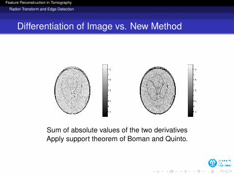
Differentiation of Image vs. New Method
Sum of absolute values of the two derivativesApply support theorem of Boman and Quinto.
Feature Reconstruction in Tomography
Radon Transform and Edge Detection
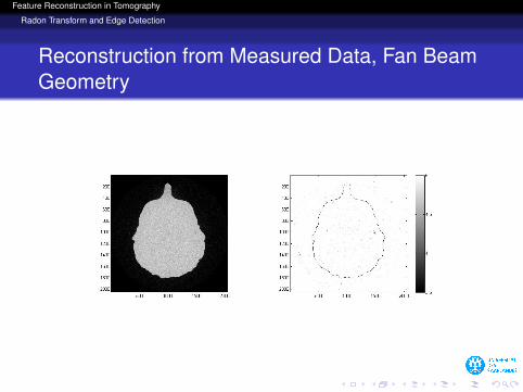
Reconstruction from Measured Data, Fan BeamGeometry
Feature Reconstruction in Tomography
Radon Transform and Edge Detection
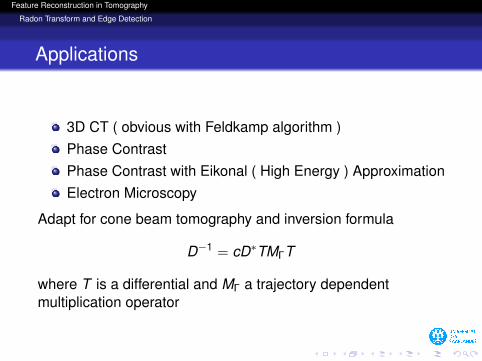
Applications
3D CT ( obvious with Feldkamp algorithm )Phase ContrastPhase Contrast with Eikonal ( High Energy ) ApproximationElectron Microscopy
Adapt for cone beam tomography and inversion formula
D−1 = cD∗TMΓT
where T is a differential and MΓ a trajectory dependentmultiplication operator
Feature Reconstruction in Tomography
Radon Transform and Diffusion
Content
1 Formulation of Problem
2 Inverse Problems and Regularization
3 Approximate Inverse for Combining Reconstruction andAnalysis
4 Radon Transform and Edge Detection
5 Radon Transform and Diffusion
6 Radon Transform and Wavelet Decomposition
7 Nonlinear Problems
8 Future
Feature Reconstruction in Tomography
Radon Transform and Diffusion
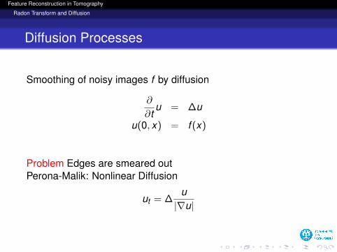
Diffusion Processes
Smoothing of noisy images f by diffusion
∂
∂tu = ∆u
u(0, x) = f (x)
Problem Edges are smeared outPerona-Malik: Nonlinear Diffusion
ut = ∆u|∇u|
Feature Reconstruction in Tomography
Radon Transform and Diffusion
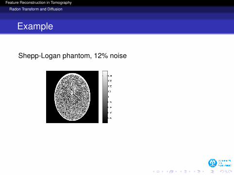
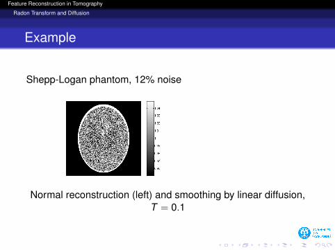
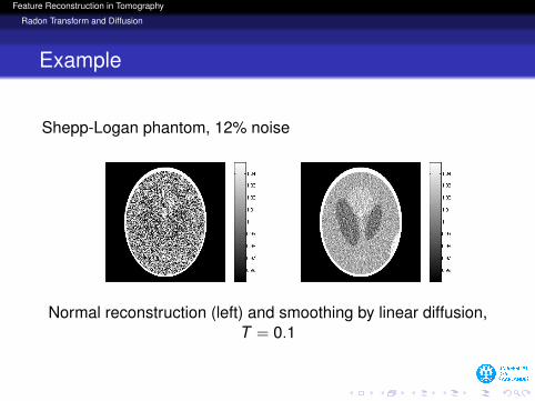
Example
Shepp-Logan phantom, 12% noise
Normal reconstruction (left) and smoothing by linear diffusion,T = 0.1
Feature Reconstruction in Tomography
Radon Transform and Diffusion
Example
Shepp-Logan phantom, 12% noise
Normal reconstruction (left) and smoothing by linear diffusion,T = 0.1
Feature Reconstruction in Tomography
Radon Transform and Diffusion
Example
Shepp-Logan phantom, 12% noise
Normal reconstruction (left) and smoothing by linear diffusion,T = 0.1
Feature Reconstruction in Tomography
Radon Transform and Diffusion
Fundamental Solution
L.: Inverse Problems and Imaging, to appear
Fundamental Solution of the heat equation
G(t , x) =1
(4πt)n/2 exp(−|x |2/4t)
The solution of the heat equation for initial conditionu(0, x) = f (x) can be calculated as
LT u(0, ·) = u(T , ·) = G(T , ·) ∗ f
Feature Reconstruction in Tomography
Radon Transform and Diffusion
Combining Reconstruction and Diffusion
Let eγ(x , ·) = δx and L = LTThen the reconstruction kernel for time t = T has to fulfil
R∗ψT (x , y) = L∗T δx (y) = G(T , x − y)
and is of convolution type.
Feature Reconstruction in Tomography
Radon Transform and Diffusion
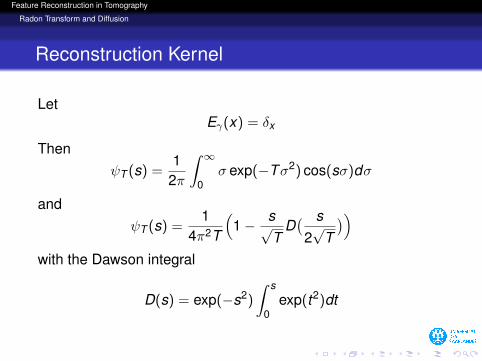
Reconstruction Kernel
LetEγ(x) = δx
ThenψT (s) =
12π
∫ ∞0
σ exp(−Tσ2) cos(sσ)dσ
andψT (s) =
14π2T
(1− s√
TD( s
2√
T
))with the Dawson integral
D(s) = exp(−s2)
∫ s
0exp(t2)dt
Feature Reconstruction in Tomography
Radon Transform and Diffusion
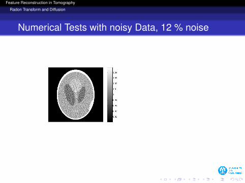
Numerical Tests with noisy Data, 12 % noise
Smoothing by linear diffusion ( left ) and combinedreconstruction (right).
Feature Reconstruction in Tomography
Radon Transform and Diffusion
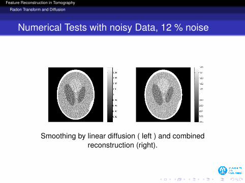
Numerical Tests with noisy Data, 12 % noise
Smoothing by linear diffusion ( left ) and combinedreconstruction (right).
Feature Reconstruction in Tomography
Radon Transform and Diffusion
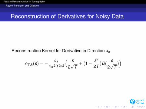
Reconstruction of Derivatives for Noisy Data
Reconstruction Kernel for Derivative in Direction xk
ψT ,k (s) = − θk
4π2T 3/2
( s2√
T+(1− s2
2T)D(
s2√
T))
Feature Reconstruction in Tomography
Radon Transform and Diffusion
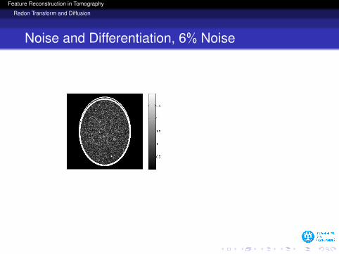
Noise and Differentiation, 6% Noise
Smoothing by linear diffusion ( left ) and combinedreconstruction (right).
Feature Reconstruction in Tomography
Radon Transform and Diffusion
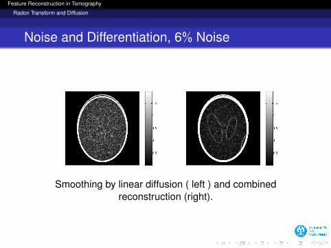
Noise and Differentiation, 6% Noise
Smoothing by linear diffusion ( left ) and combinedreconstruction (right).
Feature Reconstruction in Tomography
Radon Transform and Diffusion
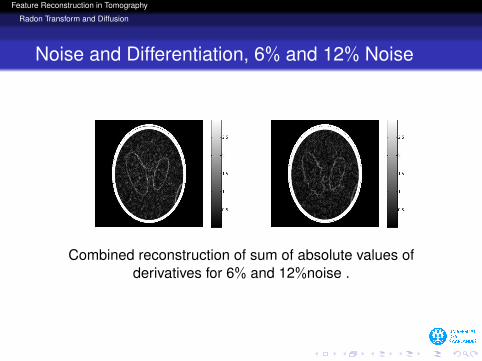
Noise and Differentiation, 6% and 12% Noise
Combined reconstruction of sum of absolute values ofderivatives for 6% and 12%noise .
No useful results with 12% noise with separate calculation ofreconstruction and smoothed derivative.
Feature Reconstruction in Tomography
Radon Transform and Diffusion
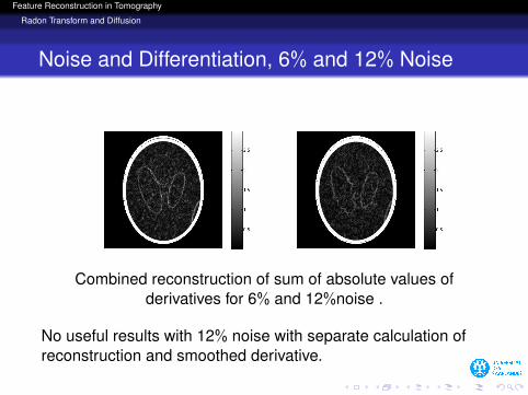
Noise and Differentiation, 6% and 12% Noise
Combined reconstruction of sum of absolute values ofderivatives for 6% and 12%noise .
No useful results with 12% noise with separate calculation ofreconstruction and smoothed derivative.
Feature Reconstruction in Tomography
Radon Transform and Wavelet Decomposition
Content
1 Formulation of Problem
2 Inverse Problems and Regularization
3 Approximate Inverse for Combining Reconstruction andAnalysis
4 Radon Transform and Edge Detection
5 Radon Transform and Diffusion
6 Radon Transform and Wavelet Decomposition
7 Nonlinear Problems
8 Future
Feature Reconstruction in Tomography
Radon Transform and Wavelet Decomposition
Wavelet Components
Combination of reconstruction and wavelet decomposition:L, Maass, Rieder, 1994Image reconstruction and wavelets :
Holschneider, 1991Berenstein, Walnut, 1996Bhatia, Karl, Willsky, 1996Bonnet, Peyrin, Turjman, 2002Wang et al, 2004
Feature Reconstruction in Tomography
Radon Transform and Wavelet Decomposition
Inversion with Wavelets
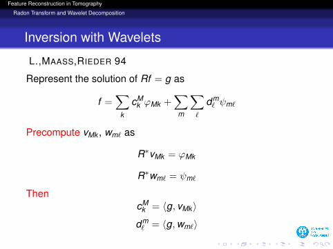
L.,MAASS,RIEDER 94
Represent the solution of Rf = g as
f =∑
k
cMk ϕMk +
∑m
∑`
dm` ψm`
Precompute vMk , wm` as
R∗vMk = ϕMk
R∗wm` = ψm`
ThencM
k = 〈g, vMk 〉
dm` = 〈g,wm`〉
Feature Reconstruction in Tomography
Radon Transform and Wavelet Decomposition
Inversion with Wavelets
L.,MAASS,RIEDER 94
Represent the solution of Rf = g as
f =∑
k
cMk ϕMk +
∑m
∑`
dm` ψm`
Precompute vMk , wm` as
R∗vMk = ϕMk
R∗wm` = ψm`
ThencM
k = 〈g, vMk 〉
dm` = 〈g,wm`〉
Feature Reconstruction in Tomography
Radon Transform and Wavelet Decomposition
Inversion with Wavelets
L.,MAASS,RIEDER 94
Represent the solution of Rf = g as
f =∑
k
cMk ϕMk +
∑m
∑`
dm` ψm`
Precompute vMk , wm` as
R∗vMk = ϕMk
R∗wm` = ψm`
ThencM
k = 〈g, vMk 〉
dm` = 〈g,wm`〉
Feature Reconstruction in Tomography
Radon Transform and Wavelet Decomposition
This is joint work with Steven OecklDepartment Process Integrated Inspection SystemsFraunhofer IIS
Feature Reconstruction in Tomography
Radon Transform and Wavelet Decomposition
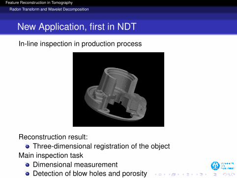
New Application, first in NDT
In-line inspection in production process
Reconstruction result:Three-dimensional registration of the object
Main inspection taskDimensional measurementDetection of blow holes and porosity
Feature Reconstruction in Tomography
Radon Transform and Wavelet Decomposition
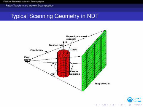
Typical Scanning Geometry in NDT
Feature Reconstruction in Tomography
Radon Transform and Wavelet Decomposition
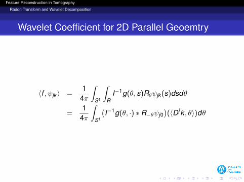
Wavelet Coefficient for 2D Parallel Geoemtry
〈f , ψjk 〉 =1
4π
∫S1
∫IR
I−1g(θ, s)Rθψjk (s)dsdθ
=1
4π
∫S1
(I−1g(θ, ·) ∗ R−θψj0
)(〈Djk , θ〉)dθ
Feature Reconstruction in Tomography
Radon Transform and Wavelet Decomposition
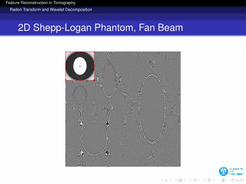
2D Shepp-Logan Phantom, Fan Beam
Feature Reconstruction in Tomography
Radon Transform and Wavelet Decomposition
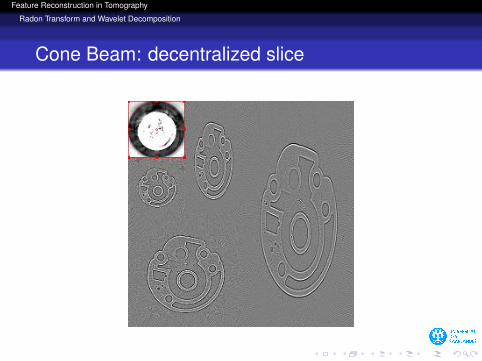
Cone Beam: decentralized slice
Feature Reconstruction in Tomography
Radon Transform and Wavelet Decomposition
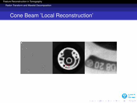
Cone Beam ’Local Reconstruction’
Feature Reconstruction in Tomography
Nonlinear Problems
Content
1 Formulation of Problem
2 Inverse Problems and Regularization
3 Approximate Inverse for Combining Reconstruction andAnalysis
4 Radon Transform and Edge Detection
5 Radon Transform and Diffusion
6 Radon Transform and Wavelet Decomposition
7 Nonlinear Problems
8 Future
Feature Reconstruction in Tomography
Nonlinear Problems
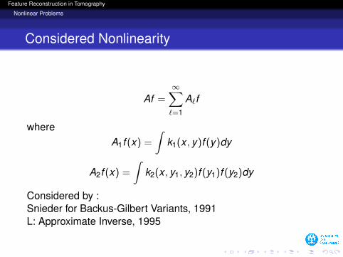
Considered Nonlinearity
Af =∞∑`=1
A`f
whereA1f (x) =
∫k1(x , y)f (y)dy
A2f (x) =
∫k2(x , y1, y2)f (y1)f (y2)dy
Considered by :Snieder for Backus-Gilbert Variants, 1991L: Approximate Inverse, 1995
Feature Reconstruction in Tomography
Nonlinear Problems
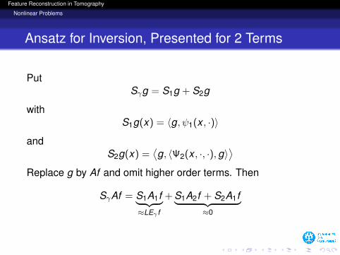
Ansatz for Inversion, Presented for 2 Terms
PutSγg = S1g + S2g
withS1g(x) = 〈g, ψ1(x , ·)〉
andS2g(x) =
⟨g, 〈Ψ2(x , ·, ·),g〉
⟩Replace g by Af and omit higher order terms. Then
SγAf = S1A1f︸ ︷︷ ︸≈LEγ f
+ S1A2f + S2A1f︸ ︷︷ ︸≈0
Feature Reconstruction in Tomography
Nonlinear Problems
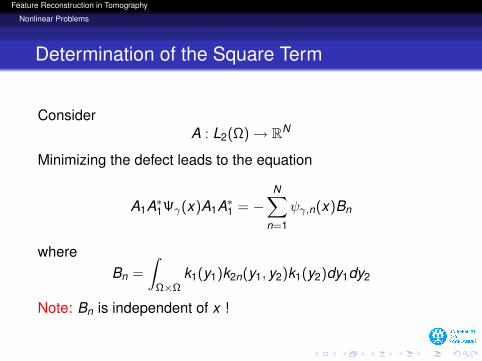
Determination of the Square Term
ConsiderA : L2(Ω)→ RN
Minimizing the defect leads to the equation
A1A∗1Ψγ(x)A1A∗1 = −N∑
n=1
ψγ,n(x)Bn
whereBn =
∫Ω×Ω
k1(y1)k2n(y1, y2)k1(y2)dy1dy2
Note: Bn is independent of x !
Feature Reconstruction in Tomography
Nonlinear Problems
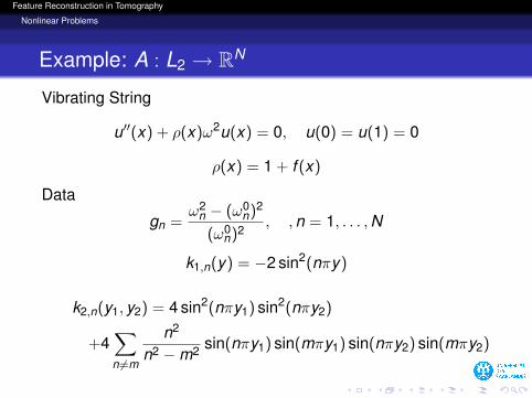
Example: A : L2 → RN
Vibrating String
u′′(x) + ρ(x)ω2u(x) = 0, u(0) = u(1) = 0
ρ(x) = 1 + f (x)
Data
gn =ω2
n − (ω0n)2
(ω0n)2
, ,n = 1, . . . ,N
k1,n(y) = −2 sin2(nπy)
k2,n(y1, y2) = 4 sin2(nπy1) sin2(nπy2)
+4∑n 6=m
n2
n2 −m2 sin(nπy1) sin(mπy1) sin(nπy2) sin(mπy2)
Feature Reconstruction in Tomography
Nonlinear Problems
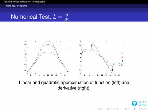
Numerical Test, L = ddx
Linear and quadratic approximation of function (left) andderivative (right).
Feature Reconstruction in Tomography
Future
Content
1 Formulation of Problem
2 Inverse Problems and Regularization
3 Approximate Inverse for Combining Reconstruction andAnalysis
4 Radon Transform and Edge Detection
5 Radon Transform and Diffusion
6 Radon Transform and Wavelet Decomposition
7 Nonlinear Problems
8 Future
Feature Reconstruction in Tomography
Future
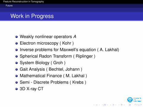
Work in Progress
Weakly nonlinear operators AElectron microscopy ( Kohr )Inverse problems for Maxwell’s equation ( A. Lakhal)Spherical Radon Transform ( Riplinger )System Biology ( Groh )Gait Analysis ( Bechtel, Johann )Mathematical Finance ( M. Lakhal )Semi - Discrete Problems ( Krebs )3D X-ray CT
Feature Reconstruction in Tomography
Future
Open Problems
Nonlinear Problems, esp. nonlinear in LTime dependent problemsother scanning geometriesother operators L

![Geometric reconstruction methods for electron tomography · Geometric tomography [13], for instance, is concerned in part with the tomographic reconstruction of homogeneous (i.e.,](https://img.pdfslide.us/doc/110x75/5f64587ea258a776be7c8806/geometric-reconstruction-methods-for-electron-tomography-geometric-tomography-13.jpg)