Embed Size (px)
Citation preview
Advanced Modeling and Uncertainty Quantification for
Flight Dynamics; Interim Results and Challenges
David C. Hyde1, Kamal M. Shweyk
2, and Frank Brown
3
Boeing Research & Technology, Huntington Beach,CA, 92646
and
Gautam Shah4
NASA Langley Research Center, Hampton VA 23681
As part of the NASA Vehicle Systems Safety Technologies (VSST), Assuring Safe and Effective Aircraft
Control Under Hazardous Conditions (Technical Challenge #3), an effort is underway within Boeing
Research and Technology (BR&T) to address Advanced Modeling and Uncertainty Quantification for Flight
Dynamics (VSST1-7). The scope of the effort is to develop and evaluate advanced multidisciplinary flight
dynamics modeling techniques, including integrated uncertainties, to facilitate higher fidelity response
characterization of current and future aircraft configurations approaching and during loss-of-control
conditions. This approach is to incorporate multiple flight dynamics modeling methods for aerodynamics,
structures, and propulsion, including experimental, computational, and analytical. Also to be included are
techniques for data integration and uncertainty characterization and quantification. This research shall
introduce new and updated multidisciplinary modeling and simulation technologies designed to improve the
ability to characterize airplane response in off-nominal flight conditions. The research shall also introduce
new techniques for uncertainty modeling that will provide a unified database model comprised of multiple
sources, as well as an uncertainty bounds database for each data source such that a full vehicle uncertainty
analysis is possible even when approaching or beyond Loss of Control boundaries. Methodologies developed
as part of this research shall be instrumental in predicting and mitigating loss of control precursors and
events directly linked to causal and contributing factors, such as stall, failures, damage, or icing. The tasks
will include utilizing the BR&T Water Tunnel to collect static and dynamic data to be compared to the GTM
extended WT database, characterizing flight dynamics in off-nominal conditions, developing tools for
structural load estimation under dynamic conditions, devising methods for integrating various modeling
elements into a real-time simulation capability, generating techniques for uncertainty modeling that draw
data from multiple modeling sources, and providing a unified database model that includes nominal plus
increments for each flight condition. This paper presents status of testing in the BR&T water tunnel and
analysis of the resulting data and efforts to characterize these data using alternative modeling methods.
Program challenges and issues are also presented.
1 Technical Fellow, Boeing Research & Technology, 5301 Bolsa Ave M/S H017-D334, AIAA Associate
Fellow. 2 Manager, Boeing Research & Technology, 5301 Bolsa Ave M/S H017-D334, AIAA Associate Fellow. 3 Aerospace Engineer, Boeing Research & Technology, 5301 Bolsa Ave M/S H017-D334, AIAA
Member. 4 Assistant Head, Flight Dynamics Branch, MS308, AIAA Senior Member
https://ntrs.nasa.gov/search.jsp?R=20140006174 2018-05-31T13:32:58+00:00Z
NOMENCLATURE
α, AOA angle of attack, deg.
β, beta angle of sideslip, deg
BR&T Boeing Research and Technology
CD drag coefficient
CL lift coefficient
CLmax maximum lift coefficient
Cl body axis rolling moment coefficient
Clp body axis roll rate damping derivative, 1/rad
Clq body axis rolling moment due to pitch rate, 1/rad.
Clr body axis rolling moment due to yaw rate, 1/rad.
Cm pitching moment
Cmp pitching moment due to roll rate, 1/rad.
Cmq pitch rate damping derivative, 1/rad
Cmr pitching moment due to yaw rate, 1/rad.
Cn body axis yawing moment coefficient
Cnp body axis yawing moment due to roll rate, 1/rad.
Cnq body axis yawing moment due to pitch rate, 1/rad
Cnr body axis yaw rate damping derivative, 1/rad.
CY side force coefficient
DOF Degree of Freedom
FVWT Flow Visualization Water Tunnel
GTM Generic Transport Model
k Strouhal number (reduced frequency), V
l
2
l Characteristic length; (b or c )
LOC Loss of Control
NAART North American Aviation Research Tunnel
p body axes roll rate, rad/sec
p̂ non-dimensional roll rate (reduced), V
pb
2, rad
q pitch rate, rad/sec
q̂ non-dimensional pitch rate (reduced), V
cq
2, rad
r body axes yaw rate, rad/sec
r̂ non-dimensional yaw rate (reduced), V
rb
2, rad
SPM Single Point Method
ω oscillation frequency; Amplitude
pmax, 1/sec
VSST Vehicle System Safety Technologies
INTRODUCTION
BACKGROUND
Reducing Loss of Control (LOC) events on commercial transport aircraft is one of the Technical
Challenges of the VSST project at NASA. Characterization of the dynamic and unsteady
behavior of aircraft during these events is a cornerstone of the project. As part of the VSST
research, BR&T is duplicating and expanding NASA’s extensive GTM dynamic derivative
database using proven methods, tools, and facilities such as the Boeing Research & Technology
(BR&T) Flow Visualization Water Tunnel (FVWT). The research will include developing,
demonstrating, and documenting new methods of analysis and integration to determine expanded
parameters of interest for characterization of steady and unsteady aerodynamic effects using
experimental data.
PURPOSE
This research will introduce new and updated multidisciplinary modeling and simulation
technologies that will improve NASA’s ability to characterize airplane response in off-nominal
flight conditions that precede and carry through LOC. The program will also introduce new
techniques for uncertainty modeling that will provide a unified database model comprised of
multiple sources, as well as an uncertainty bounds database for each data source such that a full-
vehicle uncertainty analysis is possible even when approaching or beyond LOC boundaries.
Methodologies developed as part of this research will be instrumental in predicting and
mitigating loss of control precursors and events directly linked to causal and contributing factors,
such as stall, failures, damage, or icing. Further, the flexibility of these methodologies will
ensure they are applicable to sequential precursors such that the entire event chain from initial
precursor to accident or recovery can be replicated and eventually predicted and, thus, mitigated.
The proposed work for Assuring Safe and Effective Aircraft Control under Hazardous
Conditions Technical Challenge (VSST TC-3) will improve the predictive capability for
modeling tools and methods in order to reduce the likelihood of LOC events.
The goal is to develop multi-disciplinary system modeling solutions able to predict and replicate,
and thus mitigate, sequentially occurring hazards that increase the likelihood of LOC events.
Specific research objectives include the development, evaluation, and validation of modeling
tools and methods that include:
a) Methods for characterizing the dynamic response of a vehicle in off-nominal conditions
due to steady and unsteady aerodynamic effects, propulsive effects, and aero-structural
effects;
b) Tools for structural load estimation under dynamic conditions that can be used to
estimate vehicle maneuvering limitations;
c) Development of model-validation experiments to measure the predictive capability of
experimental and computationally-derived models;

d) Methods for integration of various modeling elements (e.g., aero, structures, propulsion,
etc.) into a real-time simulation modeling capability;
e) Data fusion techniques to merge multi-source data into a unified aerodynamic database
including uncertainty;
f) Development of techniques to generate uncertainty models using real-time system
identification data;
g) Uncertainty modeling techniques able to capture both aleatory and epistemic
uncertainties; and
h) Tools and methods for propagating uncertainties in the aerodynamic database to give
bounds on vehicle system response predictions.
This paper focuses on item (a); specifically the static and forced-oscillation testing in the Boeing
FVWT and the data reduction of same, and the dynamic modeling techniques developed,
analyzed, and assessed using these data.
DESCRIPTION OF TEST FACILITIES
BOEING FLOW VISUALIZATION WATER TUNNEL
In August 1990, Rockwell International took delivery of a Water Tunnel (Model 2436) from
Eidetic Corporation, whose water tunnel manufacturing and research operations were spun off
into Rolling Hills Research Corporation in 2002. In December 1996, the Boeing Company
acquired the defense and aerospace business of Rockwell International, including what was once
North American Aviation, and, in the process, inherited the Water Tunnel. As a result of this
acquisition, Boeing also took possession of a co-located, low-speed, wind tunnel, namely the
North American Aviation Research Tunnel (NAART), built by Aerolabs, as well as a dedicated
machine shop.
As delivered, the Water Tunnel consisted of a C-strut support system with a turntable that
provided pitch and yaw control, and came equipped with six colored dye containers for flow
visualization. The closed-system, horizontal configuration of the Water Tunnel, pictured in
Figure 1, allows easy access to the model through the open top of the test section, which is 24 in.
wide by 26 in. high by 72 in. long, with tempered glass panels on all three other sides to permit
multiple viewing and recording angles. The maximum speed of the water is 1 ft/sec resulting in
a Reynold’s no. of under 100,000/ft.
In 2004 the FVWT was fitted with a 6 degree of freedom (DOF) motion rig with dynamic force
and moment measurement capabilities. In a sub-scale wind tunnel, dynamic rates are higher than
full scale rates. In a water tunnel, reduced scale and fluid velocity results in scaled dynamic
motions that are slower than full scale and sub-scale dynamic-balance wind tunnels. This yields
easier motion control and data capture, better flow visualization, negligible inertial tares, and
negligible dynamic interactions with model, hence avoiding the need for high support stiffness.
BALANCE
The FVWT has a submersible, 6 DOF, fully automated, computer controlled balance with static
and dynamic testing capabilities. The balance hardware and control software combined are called
Scorpio produced by AeroArts of Torrance, CA. The upper structure, visible in Figure 1, is
approximately seven feet high and consists of six vertical linear actuators. Below the upper
structure is a box containing the body-axis roll motor that is connected to the actuators via
carbon fiber struts. The model is mounted in front of the roll box, as illustrated in Figure 1. The
six vertical actuators and roll box together maneuver the model through the commanded motions.
Between the roll motor and the model is an adjustable pitch arc that is capable of initial position
offsets between -60 to 60 deg AOA.
GENERIC TRANSPORT MODEL
The FWVT test model was a 14% scale1 model of the NASA Generic Transport Model (GTM).
A 3-view of the model is presented in Figure 2. The GTM is a 5.5% -scale version of a generic
twin-engine, commercial transport aircraft. The test model was made using a fused deposition
modeling technique to create each part layer by layer with a continuous strip of ABS plastic
filament. The processes used a Fortus®
3D printer guided by a CAD geometry file. Some minor
hand finishing work was required to smooth the parts prior to testing.
The NASA GTM aero database and GTM Simulation aerodynamic model are based on a
dynamically scaled GTM. This model was treated as the reference basis for the FVWT test and
all data comparisons presented in this report.
SCOPE
The FVWT test consisted of static force and moment testing and dynamic forced-oscillation
testing. Dynamic runs included pitch, roll, and yaw constant frequency oscillations at multiple
frequencies and amplitudes selected to align with existing NASA GTM data. Constant-
amplitude, increasing-frequency sweeps were conducted in all axes for equivalent systems
analyses, and large-amplitude low-rate sweeps were conducted in pitch and yaw to evaluate
aerodynamic hysteresis effects. Model components with deflected control surfaces were
constructed; however, due to time constraints the model was tested in the FVWT with all
surfaces in a faired-condition only.
METHOD OF TEST
STATIC TESTING
The objectives of the static force and moment test runs for the FVWT Test were to establish a
comparison between the FVWT data and the NASA 14x22 wind tunnel data and demonstrate
repeatability of the FVWT data from similar runs conducted separately. Other research topics of
1 The 14% scale is relative to the NASA ‘AirSTAR’ scaled GTM
interest were the effects of sweep rate, flow angularity, model symmetry, and the influence of
model orientation. Pitch-pause and pitch sweep runs were conducted at similar conditions to
investigate the effect of sweep rate. During a pitch sweep, the model was continuously swept
from the lowest AOA in the schedule to the highest at a constant angular rate. For a pitch-pause
run, the model paused at each commanded AOA, typically every 2 degrees, for a period of time,
typically 50 seconds. The pitch sweeps were conducted at 0 deg beta and -16 to 30 deg AOA.
One pitch sweep was completed with the model inverted (180 deg phi), to investigate the
influence of model orientation on these data and determine flow angularity. The pitch-pause runs
were performed from -4 to 28 deg AOA, with pauses at every 2 deg AOA. Pitch-pause runs were
completed for 0, -4, and 4 deg beta, to check model symmetry. Yaw-pause runs were completed
at 0, 5, 10, and 15 deg AOA for -20 to 20 deg beta. Yaw sweeps were run in both directions at 10
deg AOA at a constant rate from -20 to 20 deg beta. One yaw sweep was run with the model
rolled 90 deg.
DYNAMIC TESTING
Constant Frequency Oscillations
Pitch, roll, and yaw oscillation runs were developed to estimate dynamic derivatives. Each series
in the matrix consisted of 12 oscillatory runs varying from -4 deg AOA to 26 deg AOA. At each
AOA, 10 oscillations were completed at a constant oscillatory frequency. The frequencies were
selected to match available GTM data from prior NASA testing.
Frequency Sweeps
Frequency sweeps were conducted in three axes, pitch, roll, and yaw at 5, 15, 25, 35, and 45 deg
AOA. The sweep runs commanded constant amplitude, increasing frequency oscillations. A tool
was developed by BR&T to determine the desired sweep frequency and amplitude prior to
testing. Constant rate (varying amplitude) frequency sweeps were also planned, but not
completed due to time constraints.
Hysteresis Sweeps
Pitch and yaw hysteresis runs commanding large amplitude oscillations at 0.4 deg/sec were
completed. The pitch hysteresis runs were designed to reach CLmax, 5 deg less than CLmax, 10
deg less than CLmax, and 15 deg less than CLmax. The yaw hysteresis runs swept from -25 to
25 deg beta at approximately 0.4 deg/sec.
RESULTS AND DISCUSSION
STATIC FORCE AND MOMENT TESTING
The static portion of FVWT testing included 15 runs focused on providing a foundation for the
oscillatory test matrix and data reduction as well as facilitating comparisons with NASA wind
tunnel data. In a typical force and moment wind tunnel test the coefficient values measured at
each angle of attack would be averaged over the time of collection and only the average value
would be preserved for analysis. In the case of this test, however, the time-history data were

preserved at the raw collection rate of 40 Hz to better assess the quality of the data to evaluate
unsteady and/or nonlinear effects. All of the reduced data presented in this report show the mean
coefficient values. The time history data are preserved in run files managed separately.
FORCE AND MOMENT DATA REPATABILITY
Force and moment repeatability was evaluated by comparing identical-condition sequential pitch
pause runs. Run repeatability results are presented for longitudinal and lateral-directional
coefficients in Figures 3 and 4 respectively. Lift coefficient repeatability was within 10%
relative error for AOA > 10 deg. Pitching moment repeatability was very good at AOAs below 9
deg and within 10% relative error for AOA>9 deg. In that standard repeatability requirements
have not been established for water tunnels as they have been for wind tunnels (Reference 1) the
acceptability of this repeatability margin could not be determined. Analysis of balance
characteristics indicates that the greatest factor affecting repeatability is likely to be the low
balance loads encountered in water tunnel testing. Typical individual and combined balance
loading for a pitch pause run are presented in Figure 5. The maximum combined load, 0.2 lbs.
represents less than 1% of the reported balance force load limits of 25 lbs for forces and 100 in-
lbs for moments.
FORCE AND MOMENT RESULTS
Force and Moment comparisons were made with available NASA wind tunnel test data. Select
comparisons for longitudinal and lateral-directional coefficients are presented in Figures 6 and 7
respectively. The comparison data is from a test in the NASA Langley 14x22 Tunnel, which was
conducted with a full-scale model of the AirSTAR GTM flight test vehicle.
FORCED OSCILLATION TESTING
The oscillatory data comprised a majority of the FVWT Test 006 data. Overall, 159 oscillatory
runs were completed. Data reduction procedures to compute dynamic derivatives via two
different methods are presented in the following sections. Data were reduced using purpose-
written MATLAB scripts and MATLAB release 2013 with no additional toolboxes or analysis
packages required. The data reduction methods were based on methods presented in Reference
2.
“SINGLE POINT” METHOD
The Single Point Method (SPM) calculated dynamic derivatives by curve fitting selected points
of the select coefficient data vs. non-dimensional oscillatory rate.
The SPM process for calculating dynamic derivatives is presented graphically in Figure 8.
Rolling moment is used in this example though the method applies to pitching and yawing
motion as well.
The SPM process consisted of the following steps:
1. ‘Detrend’ the data to remove any balance drift that occurred during the run. This is done
by fitting a 2nd
order polynomial to the moment coefficient vs. time to determine the
amount of drift over time. The drift will be subtracted out in step 4 prior to curve fitting.
2. Collect AOA, sideslip, and angular rate values at points corresponding to static
conditions within a user-specified angular rate tolerance (denoted by red circles in Figure
8). In the example presented the angular acceleration tolerance was 0 +/- 0.01 deg/sec2.
3. Smooth the moment coefficient using an 11-sample centered moving average. A study
was conducted to find an acceptable sample size that smoothed the data without
removing the peak values. 11 samples, corresponding to 0.25s at the 40 Hz data rate, was
selected.
4. The dynamic derivative, Clp in the example, is determined by linearly curve fitting the
selected points of the moment coefficient moment, less the balance drift determined in
step 1, with respect to non-dimensional rate, ̂ in the example. The second axis in Figure
8 shows the selected points, in red, and the linear curve-fit, red line. The slope of the
curve fit is the dynamic derivative in question. In this example, Clp = -0.162.
This process is repeated for each moment coefficient for each oscillatory run. The script
calculates Clx, Cmx and Cnx; where ‘x’ is the oscillatory axis p, q, or r.
“INTEGRATION” METHOD
The integration data reduction method was used to calculate dynamic derivative coefficients by
fitting a Fourier series to the moment coefficient with respect to time. The integration method is
presented graphically for a roll oscillation in Figure 9.
The integration method consisted of the following steps:
1. ‘Detrend’ the data to remove any balance drift that occurred during the run. This is done
by fitting a 2nd
order polynomial to the moment coefficient vs. time to determine the
amount of drift over time. The drift will be subtracted out in step 4 prior to curve fitting.
2. Filter the moment coefficient. All results presented in this section used an 11 sample
centered moving average. A study was conducted to determine the best smoothing span
and 11 samples, corresponding to about 0.25 sec at the 40 Hz. data rate, resulted in
smoother data without unacceptable loss of peak values.
3. Fit a first-order Fourier series to the data. The dynamic coefficient (Clp in the example
presented) is then determined from the fit according to Equation 1. Clp for the example
presented in Figure 9 is -0.177.
Where:
A1= Fourier Coefficient
k = Strouhal Number
Amplitude = Amplitude (deg.)
Equation 1
EFFECT OF BALANCE DRIFT ON OSCILLATORY DATA
An example of balance drift during a roll oscillatory run is presented in Figure 10. The first axis
shows the results of fitting yawing moment with a 1st order Fourier fit without detrending the

data. The fit models the lower frequency balance drift rather than the oscillatory motion
resulting in inaccurate dynamic derivatives. A solution to the problem of balance drift is to first
fit the coefficient time history with a linear or second order polynomial to quantify the balance
drift. The second axis in Figure 10 shows the resultant 2nd
order polynomial fit. Finally, the
dynamic derivative can be calculated by fitting the de-trended time history of the coefficient
data. The bottom axis in Figure 10 shows the results of fitting the de-trended time history.
METHOD COMPARISON VS NASA GTM WIND TUNNEL DYNAMIC DERIVATIVE
DATA
The Single Point Method has advantages and disadvantages compared with the Integration
Method. SPM is easily understood. It is easy to apply, requiring only a linear curve fit, and it is
more robust with respect to balance drift during the run. The main disadvantage is that it results
in larger confidence intervals and uses only a small portion of the collected data. The Integration
Method, in comparison, has smaller confidence intervals but is susceptible to balance drift.
Figures 11 through 13 show a comparison of the Single Point and Integration data reduction
methods vs. NASA GTM wind tunnel data for roll, pitch and yaw oscillations, respectively. The
vertical bars on each FVWT data point show the 95% confidence interval for the fit values for
each method.
Roll oscillation results, Figure 11, exhibited close agreement between the two data reduction
methods and generally good trends between the FVWT water tunnel data and NASA GTM wind
tunnel data. The vertical lines represent 95% confidence intervals for the fits involved with the
data reduction. The Integration method yields generally smaller confidence intervals by using
more of the data for the run. The Clp data trends match the NASA wind tunnel data. Cnp
matches the NASA data well up to approximately 15 degrees AOA. This trend is repeated with
other roll oscillatory series.
Pitch oscillation results, Figure 12, show very good agreement between data reduction methods
with the Integration Method having a smaller confidence interval. The Cmq data also match the
trends from the NASA wind tunnel data closely with a near constant offset throughout the angle
of attack range tested.
Yaw oscillation results, Figure 13, show good agreement with NASA data. As with other axes,
the Integration method yielded much tighter confidence intervals than the Single Point Method.
DYNAMIC MODELING
FREQUENCY-DOMAIN REPRESENTATION OF FORCED-OSCILLATION DATA
Equivalent system transfer functions were fit to constant-amplitude varying-frequency sweeps in
all three axes. Data were reduced using the SIDPAC collection of MATLAB scripts and the
methods presented in Reference 3.
The equivalent system fit process consisted of the following steps:
1. Filter output (moment coefficient) data from sweep time history. All data in this section
were filtered using a low-pass Butterworth filter to smooth the noise.
2. Remove zero-offset. The mean of the smoothed output data (smoothed moment
coefficient) was subtracted from the smoothed output data output data to reduce any
offset about zero. Note that this method did not eliminate balance drift.
3. Time-shift or trim input and output data such that output = 0 at time = 0.
4. Convert input and output signals to frequency domain (SIDPAC ‘fint’) and fit to transfer
function (SIDPAC ‘fdoe’)
The method for estimating the transfer function was generally successful where the noise was
low and there was no balance drift. Roll, pitch, and yaw results are shown in Figures 14 through
16 respectively. A typical pitch sweep is shown in Figure 15 with the preconditioning steps
before transforming into the frequency domain. Note that the maximum input frequency was
0.96 rad/sec with the frequency content falling off rapidly above that point. It is expected that a
constant rate, varying amplitude sweep would likely have better frequency content and should
result in a better transfer function fit. A second-order transfer function typically yielded the best
results, with a better match at higher frequencies where the model generated higher loads.
Data Reduction Problems
Less-than-satisfactory results were obtained when FVWT output data were questionable or of
poor quality. The data reduction process with noisy and uncorrected moment coefficient data is
presented in Figure 17. The noise in the original rolling moment data in the example presented is
not sufficiently filtered which results in flat spots at the positive and negative peaks. The drift
in the rolling moment signal can be seen as a peak of 0.7 at less than 0.1 rad/sec. The dominant
peak in the data is the drift. The resulting estimated transfer function does not match the input
data for any reasonable order of equivalent system fit.
HYSTERESIS MODELING
Large-amplitude low-rate pitch and yaw sweeps and bi-directional pitch-pause runs were
conducted in an attempt to characterize aerodynamic hysteresis in the GTM model under test. It
was expected that hysteresis, if observed, would exhibit characteristics similar to those observed
during X-48B flight testing (Figure 18). The characteristics noted, however, were not indicative
of hysteresis, instead indicating model or balance issues. Pitch-pause and sweep results for a
range of initial AOAs are presented in Figure 19. In the case of sweeps, AOA increasing is
denoted by the green traces and AOA decreasing by red traces. A single sweep consists of
increasing AOA to the predefined limit then decreasing AOA back to the initial condition. The
sweep followed a 1-cos() shape to reduce transients during direction changes. In all low-rate
large-amplitude sweep tests and bi-directional sweep tests the moments measured at the balance
did not return to their initial values when the model was returned to its initial condition. This
resulted in the characteristic loop shape seen in Figure 19. The cause of these shapes was not
determined; however, the shapes are somewhat representative of freeplay in the model mounting
system and/or possibly migration of bubbles in the model. After each immersion in the FVWT
the model was placed in a series of attitudes to allow bubbles to escape; however, their presence
cannot be ruled out completely due to these data artifacts. It must also be noted that shortly after
the hysteresis testing the balance failed and became unusable. The effect of intermittent failure
or balance degradation prior to failure on the hysteresis sweep data could not be determined.
STRIP THEORY MODELING
Dynamic derivatives were also estimated using strip theory as presented in Reference 4. In this
method the contribution of individual model components to dynamic derivatives is estimated
based on static (force and moment) characteristics. These contributions can then be summed to
form an estimate of six dynamic derivates. In this evaluation component contributions were
based on (in descending order of priority): NASA static data, FVWT static data, and vortex-
lattice methods. If component characteristics were not available from a particular source, the
next-lowest priority source data were used. Results for three primary damping terms (roll, pitch,
and yaw) are presented in Figure 20, and are compared to NASA data and results generated by
the vortex lattice tool while developing supplementing static data. Best agreement was achieved
in the roll axis which agreed well with NASA data. The other damping terms (pitch and yaw)
did not show good agreement but were of similar orders of magnitude. It was noted that the best
agreement came from the axis which required the least supplemental data from the linear vortex
lattice estimates. It is expected that agreement will improve in the other axes with better static
data to use with the strip method. In the interim, however, strip theory provided a reasonable
estimation method for first-order estimates of airplane characteristics without the added expense
of additional testing to obtain forced-oscillation data.
CONCLUSIONS
FORCE AND MOMENT DATA
Force and moment testing in the BR&T FVWT resulted in mismatches between test data and the
test basis. These mismatches can be attributed to balance loading and resolution, differences in
scale and Reynolds Number, and the data trended similarly when compared to NASA wind
tunnel data. Additional testing to further evaluate balance loading and resolution effects with an
improved balance are planned for CY2014.
OSCILLATORY DATA
The FVWT has proven to be a low cost method for obtaining dynamic derivative data compared
to flight testing and wind tunnel testing. Roll, pitch and yaw oscillation data was successfully
reduced via two different methods using MATLAB based data reduction scripts written to
accomplish the task efficiently. The oscillatory data compares favorably with NASA wind
tunnel data.
Additional data collection efforts were delayed due to an issue with the water tunnel balance.
These tests will be completed when the balance is repaired or replaced.
DYNAMIC MODELING
These tests and analysis demonstrated the frequency domain technique of an equivalent system
fit to capture the frequency dependencies of dynamic aerodynamic terms. Also confirmed was
the applicability of strip theory for preliminary estimates of airplane dynamic derivatives.
Hysteresis modeling efforts were inconclusive due to questionable test results. Additional
testing with frequency sweeps designed to increase the frequency content of the resulting
moments, and to reevaluate hysteresis characteristics with an improved balance are planned for
CY2014.
REFERENCES
1. Barlow, J., Rae, W. H., and Pope, A., Low Speed Wind Tunnel Testing third edition
ISBN 9788126525683
2. Vicroy, D.D; Daniel G. Murri, D. G.; and Grafton, S. B., ” Low-speed Dynamic Force Tests
of a Subsonic Blended-Wing-Body Tri-jet Configuration”, NASA/TM—2010–216198,2010
3. Murphy, P. C., Klein, V.: Validation of Methodology for Estimating Aircraft Unsteady
Aerodynamic Parameters from Dynamic Wind Tunnel Tests, AIAA Paper 2003-5397,
August 2003.
4. Wykes, J. H. et. al; “An Analytical Study of the Dynamics of Spinning Aircraft”, WADC
Technical Report 58-381, December 1958
Figure 1. Boeing’s Dynamic FVWT
Figure 2: FVWT Generic Transport Test Model
Figure 3: Longitudinal Force and Moment repeatability for back to back repeat runs.
Figure 4: Lateral Force and Moment repeatability for back to back repeat runs
-5 0 5 10 15 20 25-0.5
0
0.5
1
, deg
CL
-5 0 5 10 15 20 25-0.5
0
0.5
1
1.5
, deg
CD
-5 0 5 10 15 20 25-0.6
-0.4
-0.2
0
0.2
, deg
Cm
GT M Test 06 Run 1 Beta 0.0 pit ch pause
GT M Test 06 Run 2 Beta 0.0 pit ch pause
FVWT Test 6 GTM Force and Moment Repeatability
Longitudinal Coefficients
Script: QGTMcompareFMVsNASA Date: 2013-08-08 08:55:38
-5 0 5 10 15 20 25-5
0
5
10x 10
-3
, deg
Cl
-5 0 5 10 15 20 25-5
0
5
10
15x 10
-3
, deg
Cn
-5 0 5 10 15 20 25-0.05
0
0.05
0.1
0.15
0.2
, deg
CY
GT M Test 06 Run 1 Beta 0.0 pit ch pause
GT M Test 06 Run 2 Beta 0.0 pit ch pause
FVWT Test 6 GTM Force and Moment Repeatability
Lateral Coefficients
Script: QGTMcompareFMVsNASA Date: 2013-08-08 09:55:42
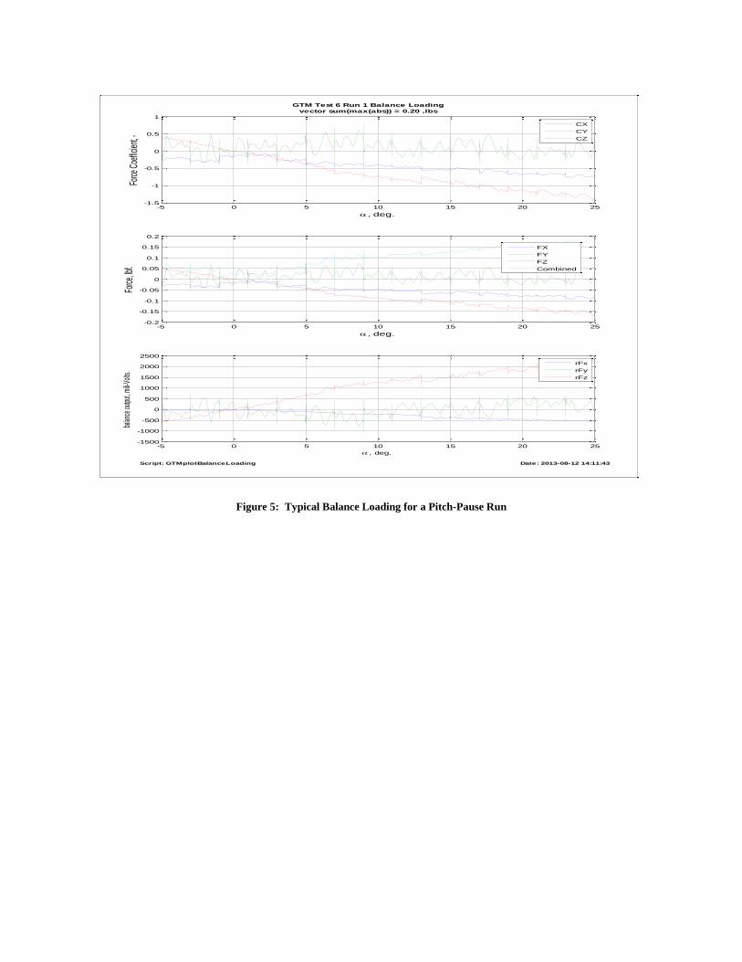
Figure 5: Typical Balance Loading for a Pitch-Pause Run
-5 0 5 10 15 20 25-1.5
-1
-0.5
0
0.5
1
, deg.
Force
Coe
fficien
t, -
CX
CY
CZ
-5 0 5 10 15 20 25-0.2
-0.15
-0.1
-0.05
0
0.05
0.1
0.15
0.2
, deg.
Force
, lbf.
FX
FY
FZ
Combined
-5 0 5 10 15 20 25-1500
-1000
-500
0
500
1000
1500
2000
2500
, deg.
balan
ce ou
tput,
mili-V
olts.
rFx
rFy
rFz
GTM Test 6 Run 1 Balance Loading
vector sum(max(abs)) = 0.20 ,lbs
Script: GTMplotBalanceLoading Date: 2013-08-12 14:11:43

Figure 6: Longitudinal Comparison with NASA Wind Tunnel Data
Figure 7: Lateral Comparison with NASA Wind Tunnel Data
-5 0 5 10 15 20 25-0.6
-0.4
-0.2
0
0.2
0.4
0.6
0.8
1
1.2
, deg
CL
-5 0 5 10 15 20 25-0.8
-0.6
-0.4
-0.2
0
0.2
0.4
0.6
, deg
Cm
GT M Test 06 Run 1 Beta 0.0 pit ch pause
GT M Test 06 Run 2 Beta 0.0 pit ch pause
NASA GTM Test 128 Run 43 Beta 0.0
FVWT Test 6 GTM Force and Moment Longitudinal Comparison
with NASA Data; Beta = 0
Script: QGTMcompareFMVsNASA Date: 2013-08-08 12:38:32
-5 0 5 10 15 20 25-5
0
5
10
15x 10
-3
, deg
Cn
-5 0 5 10 15 20 25-5
0
5
10x 10
-3
, deg
Cl
-5 0 5 10 15 20 25-0.05
0
0.05
0.1
0.15
0.2
, deg
CY
GT M Test 06 Run 1 Beta 0.0 pit ch pause
GT M Test 06 Run 2 Beta 0.0 pit ch pause
NASA GTM Test 128 Run 43 Beta 0.0
FVWT Test 6 GTM Force and Moment Lateral Comparison
with NASA Data; Beta = 0
Script: QGTMcompareFMVsNASA Date: 2013-08-08 12:43:08

Figure 8: Example Clp calculation using the single point method.
Figure 9: Example Clp calculation using the integration method.
-0.04 -0.03 -0.02 -0.01 0 0.01 0.02 0.03 0.04-0.01
-0.005
0
0.005
0.01
0.015
0.02
p̂
Cl
fit r2= 0.8958
-20 0 20 40 60 80 100 120 140 160-10
-8
-6
-4
-2
0
2
4
6
8
10
time, sec.
,de
g.
GT M Test 6 Run 25 Alpha 10 Accel Tolerance 0.010 Freq (Hz) 0.069
Single Point Data Reduction Method
Clp = -0.162
11 sample moving average on Cl
Script: QDR_SinglePoint_t006 Date: 2013-07-15 14:40:44
-20 0 20 40 60 80 100 120 140 160-10
-8
-6
-4
-2
0
2
4
6
8
10
time, sec.
,deg.
-20 0 20 40 60 80 100 120 140 160-0.01
-0.005
0
0.005
0.01
0.015
0.02
time, sec.
Cl
measured data
fit r2= 0.8868
GT M Test 6 Run 25 Alpha 10 Accel Tolerance 0.010 Freq (Hz) 0.069
Integration Method Data Reduction Method
Clp = -0.177
11 sample moving average on Cl
Script: QDR_SinglePoint_t006 Date: 2013-07-15 14:40:45
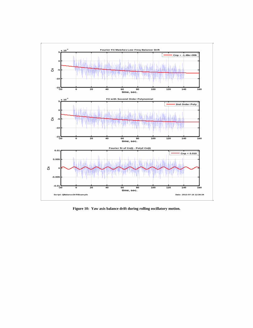
Figure 10: Yaw axis balance drift during rolling oscillatory motion.
-20 0 20 40 60 80 100 120 140 160-15
-10
-5
0
5x 10
-3
time, sec.
Cn
Fourier Fit Matches Low Freq Balance Drift
Cnp = -1.48e+006
-20 0 20 40 60 80 100 120 140 160-15
-10
-5
0
5x 10
-3
time, sec.
Cn
Fit with Second Order Polynomial
2nd Order Poly
-20 0 20 40 60 80 100 120 140 160-0.01
-0.005
0
0.005
0.01
time, sec.
Cn
Fourier fit of Cn(t) - Poly2 Cn(t)
Cnp = 0.010
Script: QBalanceDriftExample Date: 2013-07-15 12:30:34
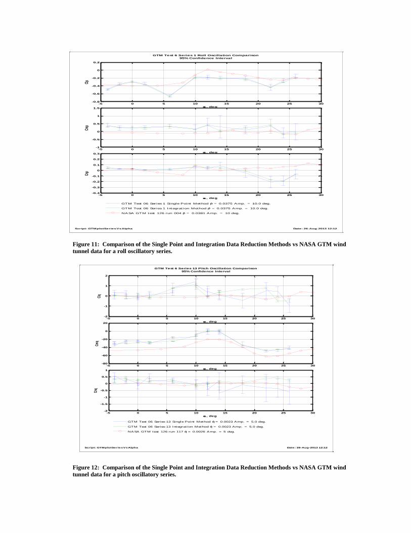
Figure 11: Comparison of the Single Point and Integration Data Reduction Methods vs NASA GTM wind
tunnel data for a roll oscillatory series.
Figure 12: Comparison of the Single Point and Integration Data Reduction Methods vs NASA GTM wind
tunnel data for a pitch oscillatory series.
-5 0 5 10 15 20 25 30-0.8
-0.6
-0.4
-0.2
0
0.2
, deg
Clp
-5 0 5 10 15 20 25 30-1
-0.5
0
0.5
1
1.5
, deg
Cmp
-5 0 5 10 15 20 25 30-0.4
-0.3
-0.2
-0.1
0
0.1
0.2
0.3
, deg
Cnp
GTM Test 06 Series 1 Single Point Method p̂ = 0.0375 Amp. = 10.0 deg.
GTM Test 06 Series 1 Integrat ion Method p̂ = 0.0375 Amp. = 10.0 deg.
NASA GTM test 126 run 004 p̂ = 0.0381 Amp. = 10 deg.
GTM Test 6 Series 1 Roll Oscillation Comparison
95% Confidence Interval
Script: GTMplotSeriesVsAlpha Date: 26-Aug-2013 12:12
-5 0 5 10 15 20 25 30-2
-1
0
1
2
, deg
Clq
-5 0 5 10 15 20 25 30-80
-60
-40
-20
0
20
, deg
Cmq
-5 0 5 10 15 20 25 30-2
-1.5
-1
-0.5
0
0.5
1
, deg
Cnq
GTM Test 06 Series 13 Single Point Method q̂ = 0.0023 Amp. = 5.0 deg.
GTM Test 06 Series 13 Integrat ion Method q̂ = 0.0023 Amp. = 5.0 deg.
NASA GTM test 126 run 117 q̂ = 0.0026 Amp. = 5 deg.
GTM Test 6 Series 13 Pitch Oscillation Comparison
95% Confidence Interval
Script: GTMplotSeriesVsAlpha Date: 26-Aug-2013 12:12
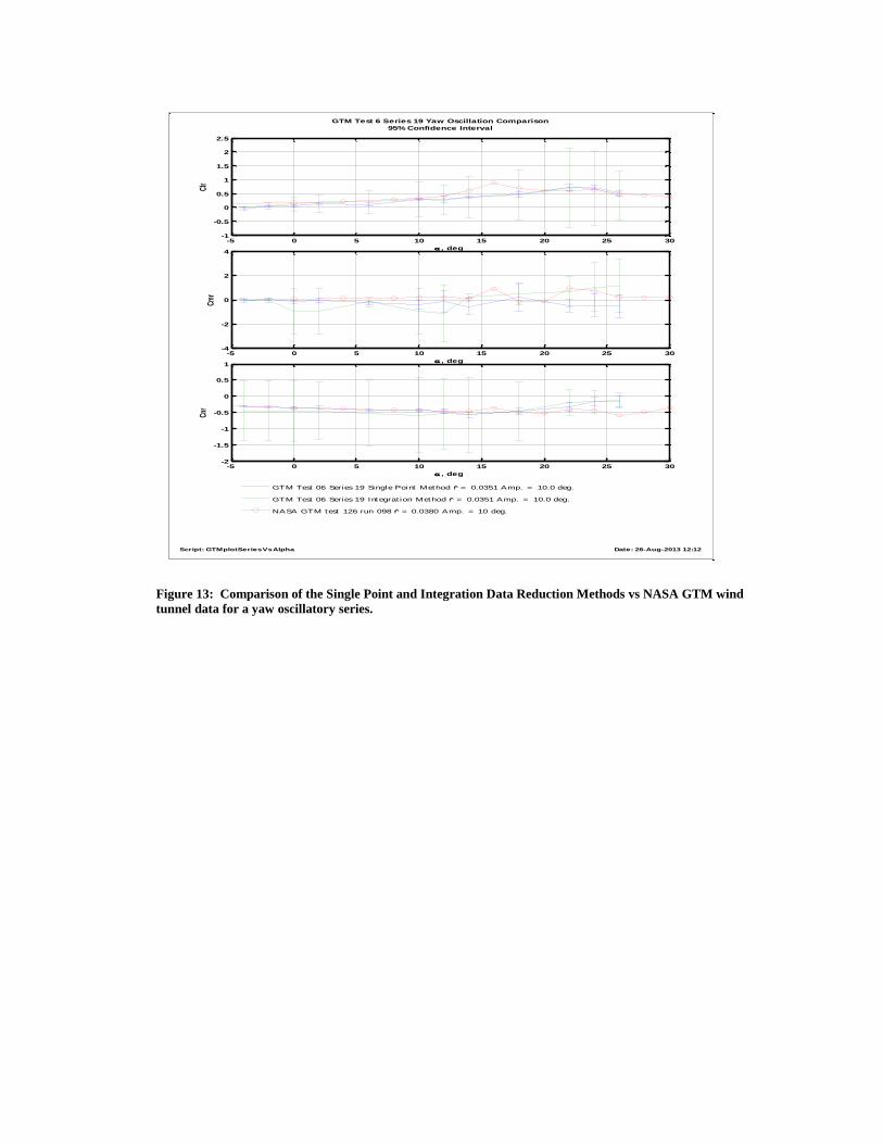
Figure 13: Comparison of the Single Point and Integration Data Reduction Methods vs NASA GTM wind
tunnel data for a yaw oscillatory series.
-5 0 5 10 15 20 25 30-1
-0.5
0
0.5
1
1.5
2
2.5
, deg
Clr
-5 0 5 10 15 20 25 30-4
-2
0
2
4
, deg
Cmr
-5 0 5 10 15 20 25 30-2
-1.5
-1
-0.5
0
0.5
1
, deg
Cnr
GTM Test 06 Series 19 Single Point Method r̂ = 0.0351 Amp. = 10.0 deg.
GTM Test 06 Series 19 Integrat ion Method r̂ = 0.0351 Amp. = 10.0 deg.
NASA GTM test 126 run 098 r̂ = 0.0380 Amp. = 10 deg.
GTM Test 6 Series 19 Yaw Oscillation Comparison
95% Confidence Interval
Script: GTMplotSeriesVsAlpha Date: 26-Aug-2013 12:12
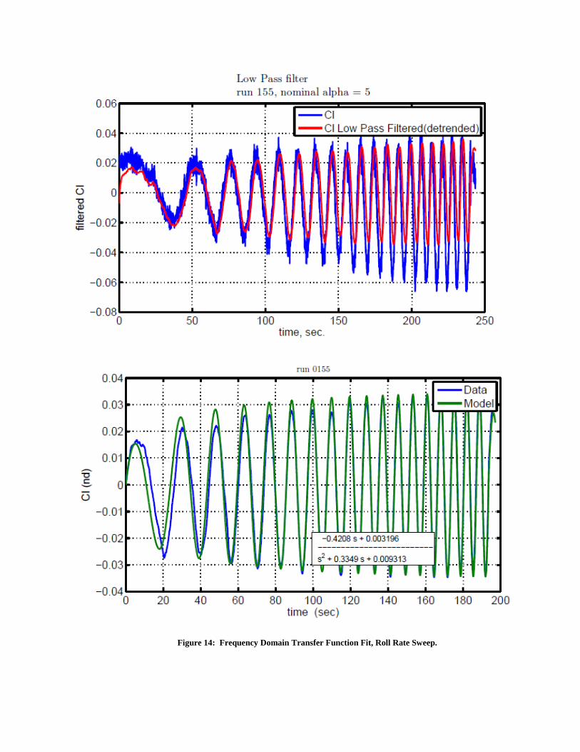
Figure 14: Frequency Domain Transfer Function Fit, Roll Rate Sweep.
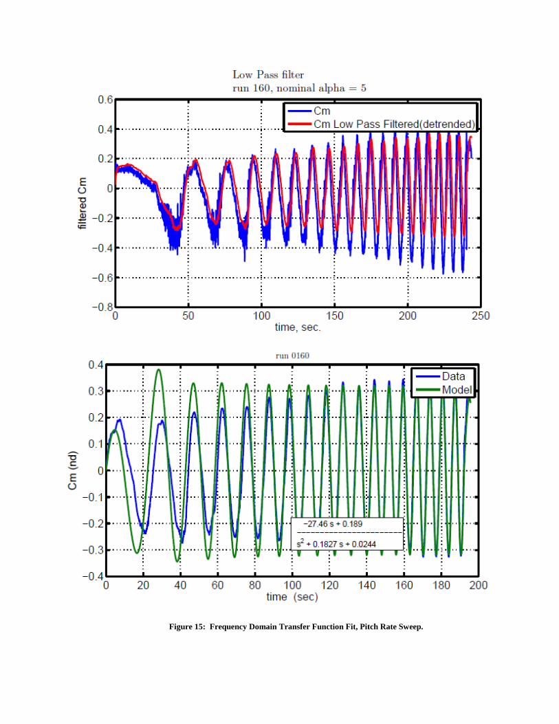
Figure 15: Frequency Domain Transfer Function Fit, Pitch Rate Sweep.
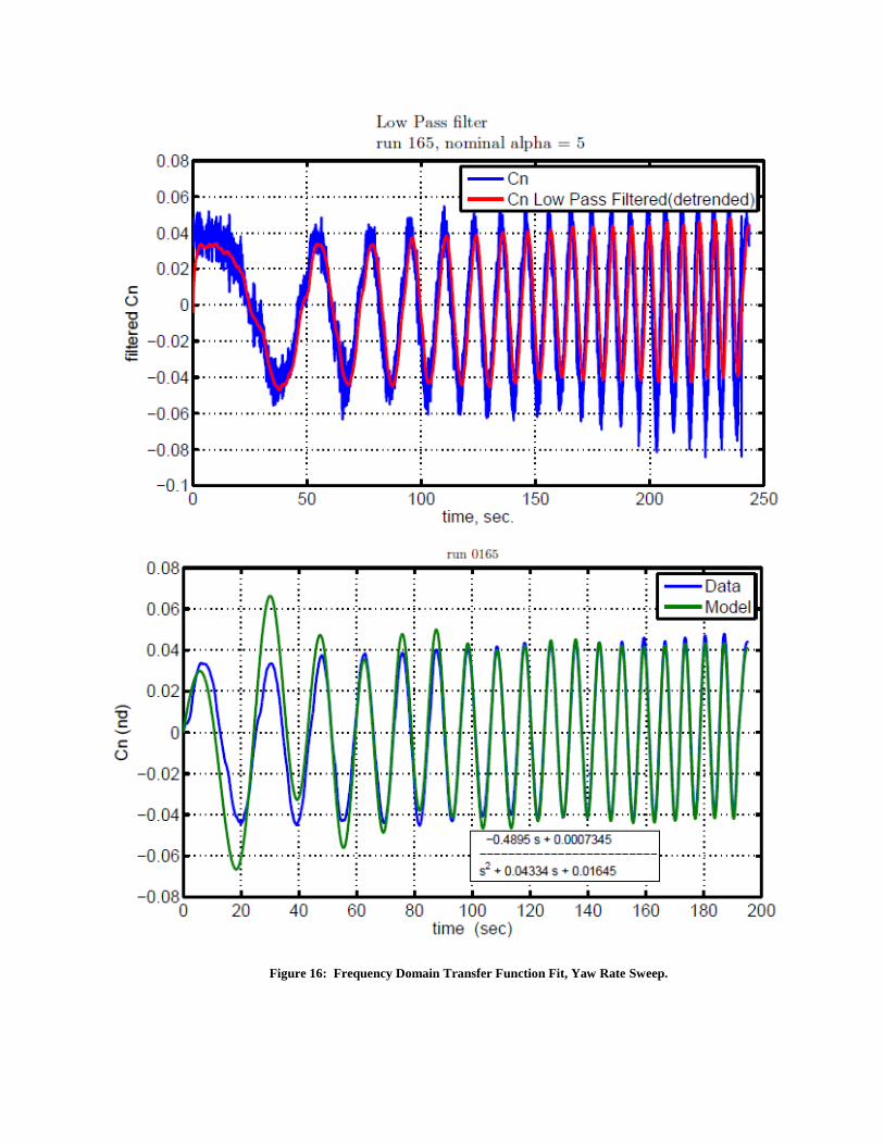
Figure 16: Frequency Domain Transfer Function Fit, Yaw Rate Sweep.
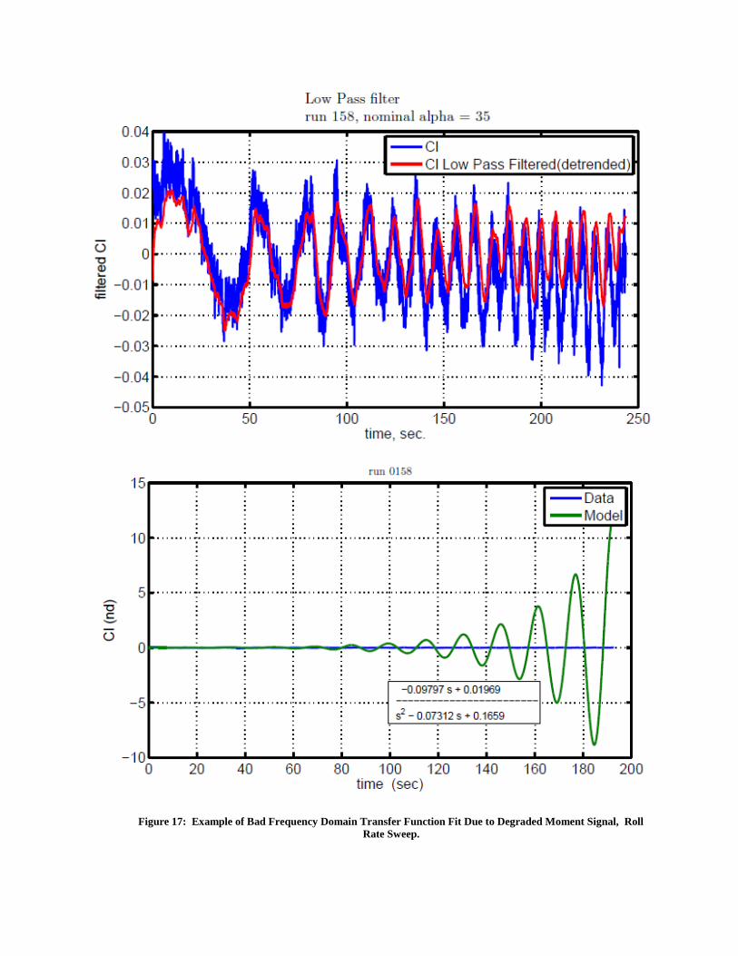
Figure 17: Example of Bad Frequency Domain Transfer Function Fit Due to Degraded Moment Signal, Roll
Rate Sweep.
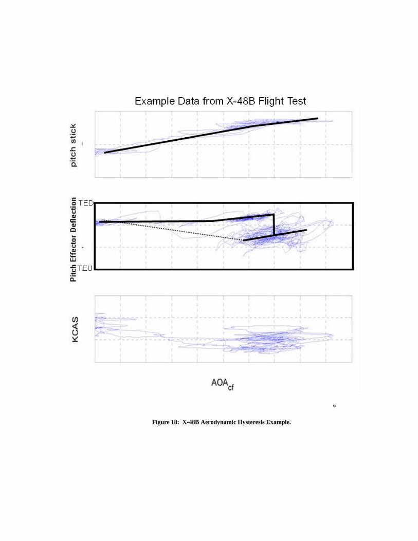
Figure 18: X-48B Aerodynamic Hysteresis Example.
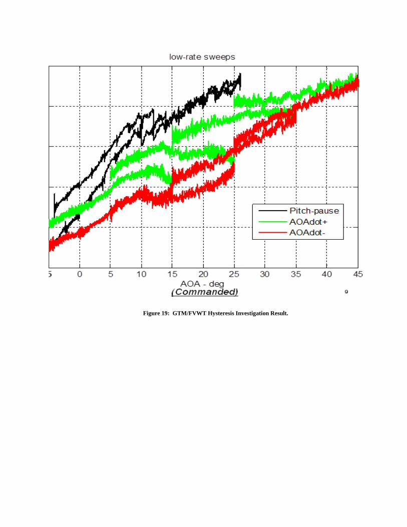
Figure 19: GTM/FVWT Hysteresis Investigation Result.
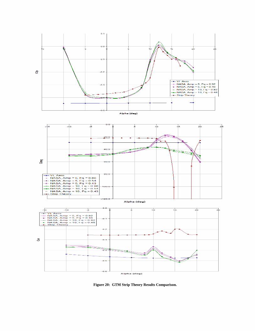
Figure 20: GTM Strip Theory Results Comparison.