1

Advanced Microeconomics

Consumer Functions Note: all of these are homogenous of degree zero with respect to p,m or just p (for Hicksian). The

exception is the expenditure function, which is homogenous of degree one in p.

Direct Utility Function The direct utility function is derived from the underlying consumer preferences. Its properties can be

derived from particular assumptions that are made about those preferences.

Marshallian Demand Function Marshallian demand functions are the solutions to the utility maximization problem:

It maximises utility subject to a fixed income.

Indirect Utility Function Indirect utility is found by substituting marshallian demand back into the utility function:

Hicksian Demand Function Hicksian demand functions are the solutions to the expenditure minimization problem:

It minimizes expenditure subject to a fixed utility (compensated demand).

Expenditure Function The expenditure function is found by multiplying the hicksian demand function by prices:

This describes the minimum amount of money an individual needs to achieve some level of utility,

given a utility function and prices.

Aggregation Across Consumers In order for us to be able to aggregate individual consumer demands for a particular good, consumer

demands must meet certain conditions. This condition can be expressed as follows:

This means that it must be the case that the sum of the demands for good of two consumers

would be equal to the demand for by a hypothetical third consumer who earned the sum of their

incomes.

This in turn requires that consumer demand be linear in income (of the Gorman Form):

2

Where and are both functions of prices and not income. It also must be true that is

shared between individuals, while may be different.

One common and convenient representation of indirect utility functions that satisfy this criterion is

known as the Gorman Polar Form, which is:

With the following definitions applying to the demand for good :

The Gorman form is necessary in order to treat a society of utility-maximizing individuals as a single

(representative) individual. This is because under the Gorman form, income effects are identical for

all consumers, and constant with increasing income (check this by differentiating marshallian

demand with respect to income).

Aggregation Across Goods Aggregation over goods is necessary if we want to simplify a problem by looking at only a few

relative prices. Much of the time we are interested in one or two specific goods and another

aggregate we call “other goods”. The theorem associated with this can be stated as follows:

When the prices of a group of commodities move in parallel, then the total expenditure on the

corresponding group of commodities can be treated as a single good.

The price and quantity of this composite good can be defined as follows:

Where is a scalar that represents the proportional increase in prices over their initial level .

Investigating Consumer Functions

Shephard’s Lemma

Roy’s Identity

Money Metric Utility Function

3

Four Identities The minimum expenditure needed to reach the maximum utility attainable at is .

The maximum utility from the minimum income needed to attain utility is .

The marshallian demand at income is the same as the hicksian demand at utility

The hicksian demand at utility is the same as the marshallian demand at income

Slutsky Equation

If is the marshallian demand function and is the hicksian demand function then:

We can also do this for a cross-price version:

Slutsky Matrix The expenditure function is concave, meaning that its second derivatives are always negative. The

second derivatives of the expenditure function are equal to the derivatives of the Hicksian demand

function, which is exactly what is put in the Slutsky matrix. This the diagonal terms of the Slutsky

matrix must be negative, which in turn means that the Slutsky matrix is negative definite.

Substitutes and Complements Gross includes both income and substitution effects, whereas net includes only substitution effects.

Gross Complements:

Gross Substitutes:

4

Net Complements:

Net Substitutes:

Elasticities

Consumer Welfare

Compensating Variation Compensating variation (CV ) is the change in income at the new prices that would be necessary to

compensate the consumer for a change in the price such that they stay on the same utility curve as

before. Thus:

This can also be expressed as follows

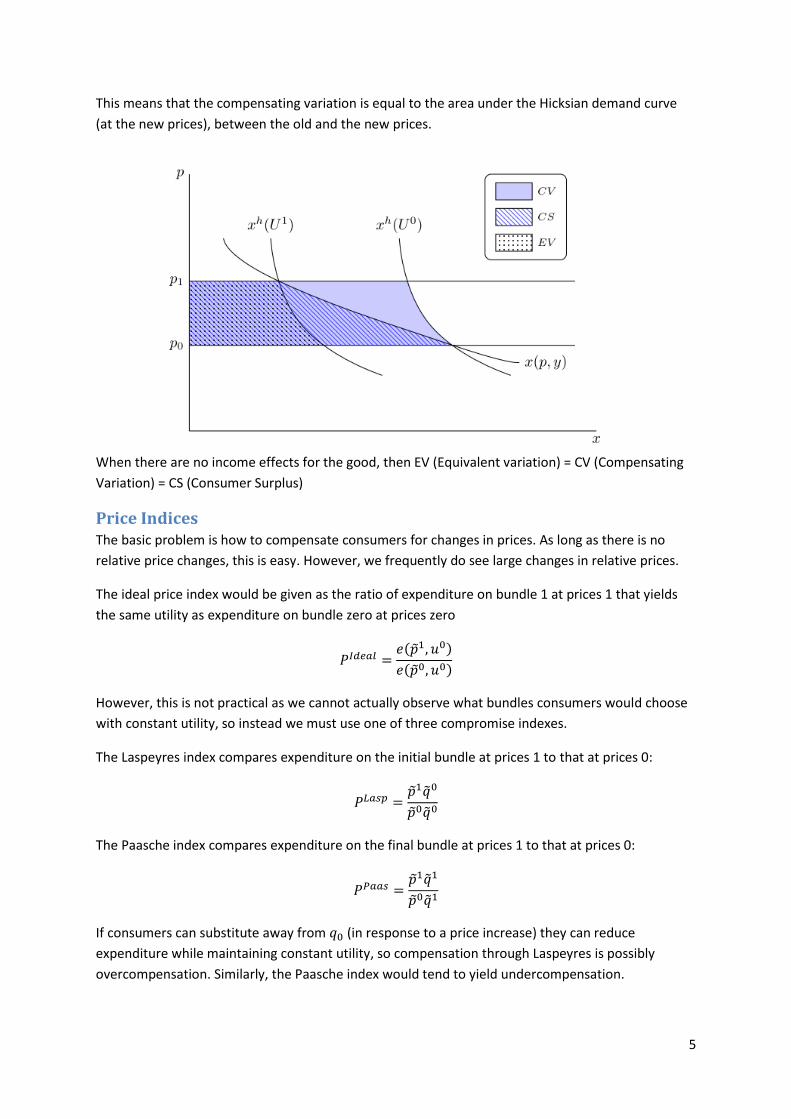
This means that the compensating variation is equal to the area under the Hicksian demand curve

(at the old prices), between the old and the new prices.

Equivalent Variation Equivalent variation is very similar to compensating variation, except that it measures the amount of

money the consumer would be willing to pay at the old prices to avoid the price change. This means

that the reference prices are rather than .

This can also be expressed as follows

5

This means that the compensating variation is equal to the area under the Hicksian demand curve

(at the new prices), between the old and the new prices.

When there are no income effects for the good, then EV (Equivalent variation) = CV (Compensating

Variation) = CS (Consumer Surplus)

Price Indices The basic problem is how to compensate consumers for changes in prices. As long as there is no

relative price changes, this is easy. However, we frequently do see large changes in relative prices.

The ideal price index would be given as the ratio of expenditure on bundle 1 at prices 1 that yields

the same utility as expenditure on bundle zero at prices zero

However, this is not practical as we cannot actually observe what bundles consumers would choose

with constant utility, so instead we must use one of three compromise indexes.

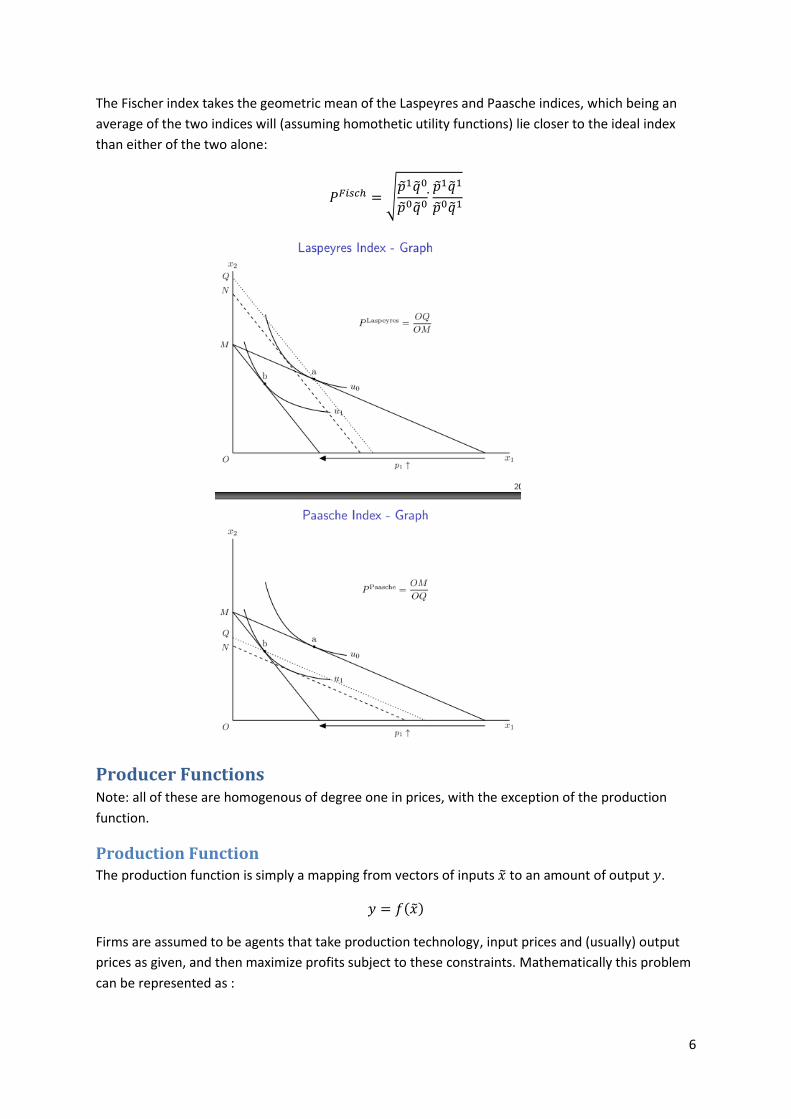
The Laspeyres index compares expenditure on the initial bundle at prices 1 to that at prices 0:

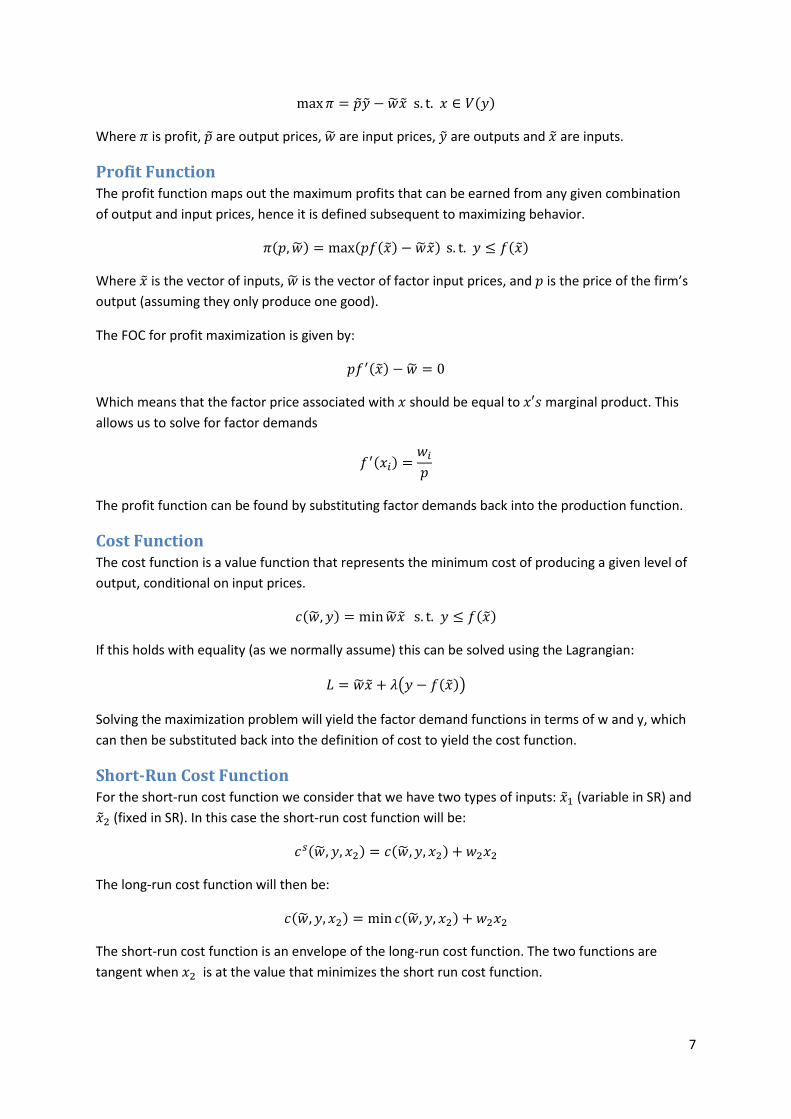
The Paasche index compares expenditure on the final bundle at prices 1 to that at prices 0:

If consumers can substitute away from (in response to a price increase) they can reduce

expenditure while maintaining constant utility, so compensation through Laspeyres is possibly

overcompensation. Similarly, the Paasche index would tend to yield undercompensation.

6

The Fischer index takes the geometric mean of the Laspeyres and Paasche indices, which being an

average of the two indices will (assuming homothetic utility functions) lie closer to the ideal index

than either of the two alone:

Producer Functions Note: all of these are homogenous of degree one in prices, with the exception of the production

function.

Production Function The production function is simply a mapping from vectors of inputs to an amount of output .

Firms are assumed to be agents that take production technology, input prices and (usually) output

prices as given, and then maximize profits subject to these constraints. Mathematically this problem

can be represented as :

7

Where is profit, are output prices, are input prices, are outputs and are inputs.

Profit Function The profit function maps out the maximum profits that can be earned from any given combination

of output and input prices, hence it is defined subsequent to maximizing behavior.

Where is the vector of inputs, is the vector of factor input prices, and is the price of the firm’s

output (assuming they only produce one good).

The FOC for profit maximization is given by:

Which means that the factor price associated with should be equal to marginal product. This

allows us to solve for factor demands

The profit function can be found by substituting factor demands back into the production function.

Cost Function The cost function is a value function that represents the minimum cost of producing a given level of

output, conditional on input prices.

If this holds with equality (as we normally assume) this can be solved using the Lagrangian:

Solving the maximization problem will yield the factor demand functions in terms of w and y, which

can then be substituted back into the definition of cost to yield the cost function.

Short-Run Cost Function For the short-run cost function we consider that we have two types of inputs: (variable in SR) and

(fixed in SR). In this case the short-run cost function will be:

The long-run cost function will then be:

The short-run cost function is an envelope of the long-run cost function. The two functions are

tangent when is at the value that minimizes the short run cost function.

8

Revenue Function The revenue function gives the maximum revenue that can be earned given prices and fixed

endowments (e.g. given level of capital and labour). In other words, the firm takes prices and

endowments as given and decides how much of each output to maximize revenue.

Investigating Producer Functions

Hotelling’s Lemma If the profit function is differentiable in p and w, the unique profit maximising supply and derived

demand functions are given as:

This result follows naturally from the envelope theorem.

Shephard’s Lemma Again Applied to the producer case, this states that the derivative of the cost function c(w,y) with respect

to the factor price is equal to the factor demands for that input conditional upon producing output y

This is essentially another application of the envelope principle.

Technical Rate of Substitution The technical rate of substitution between inputs as defined as:

The MRTS can also be seen as the slope of an isoquant at the point in question.

Separability of Inputs The cost function is weakly separable if the ratio of two related (i.e. for similar inputs) factor

demands and is not affected by changes in a third price .

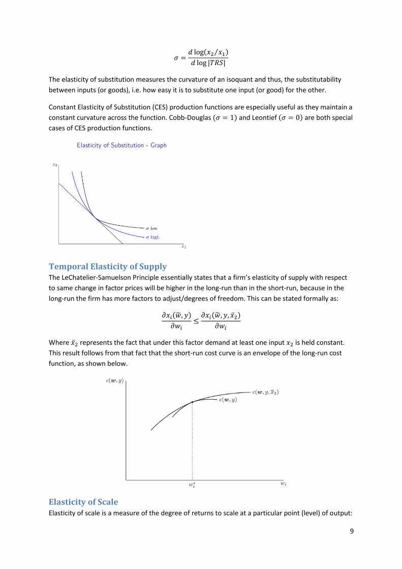
Elasticity of Substitution The elasticity of substitution is equal to the percentage change in the ratio of inputs divided by the

percentage change in the TRS that occurs as a result of this change:

9

The elasticity of substitution measures the curvature of an isoquant and thus, the substitutability

between inputs (or goods), i.e. how easy it is to substitute one input (or good) for the other.

Constant Elasticity of Substitution (CES) production functions are especially useful as they maintain a

constant curvature across the function. Cobb-Douglas and Leontief are both special

cases of CES production functions.

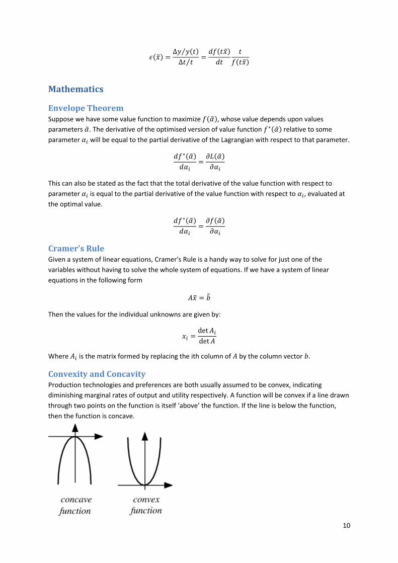
Temporal Elasticity of Supply The LeChatelier-Samuelson Principle essentially states that a firm’s elasticity of supply with respect

to same change in factor prices will be higher in the long-run than in the short-run, because in the

long-run the firm has more factors to adjust/degrees of freedom. This can be stated formally as:

Where represents the fact that under this factor demand at least one input is held constant.

This result follows from that fact that the short-run cost curve is an envelope of the long-run cost

function, as shown below.

Elasticity of Scale Elasticity of scale is a measure of the degree of returns to scale at a particular point (level) of output:

10

Mathematics

Envelope Theorem Suppose we have some value function to maximize , whose value depends upon values

parameters . The derivative of the optimised version of value function relative to some

parameter will be equal to the partial derivative of the Lagrangian with respect to that parameter.

This can also be stated as the fact that the total derivative of the value function with respect to

parameter is equal to the partial derivative of the value function with respect to , evaluated at

the optimal value.

Cramer’s Rule Given a system of linear equations, Cramer's Rule is a handy way to solve for just one of the

variables without having to solve the whole system of equations. If we have a system of linear

equations in the following form

Then the values for the individual unknowns are given by:

Where is the matrix formed by replacing the ith column of by the column vector .

Convexity and Concavity Production technologies and preferences are both usually assumed to be convex, indicating

diminishing marginal rates of output and utility respectively. A function will be convex if a line drawn

through two points on the function is itself ‘above’ the function. If the line is below the function,

then the function is concave.

11

Test: The weighted average of the function evaluated at two points is greater (convex) or lesser

(concave) than the function evaluated at the same weighted average of those two points.

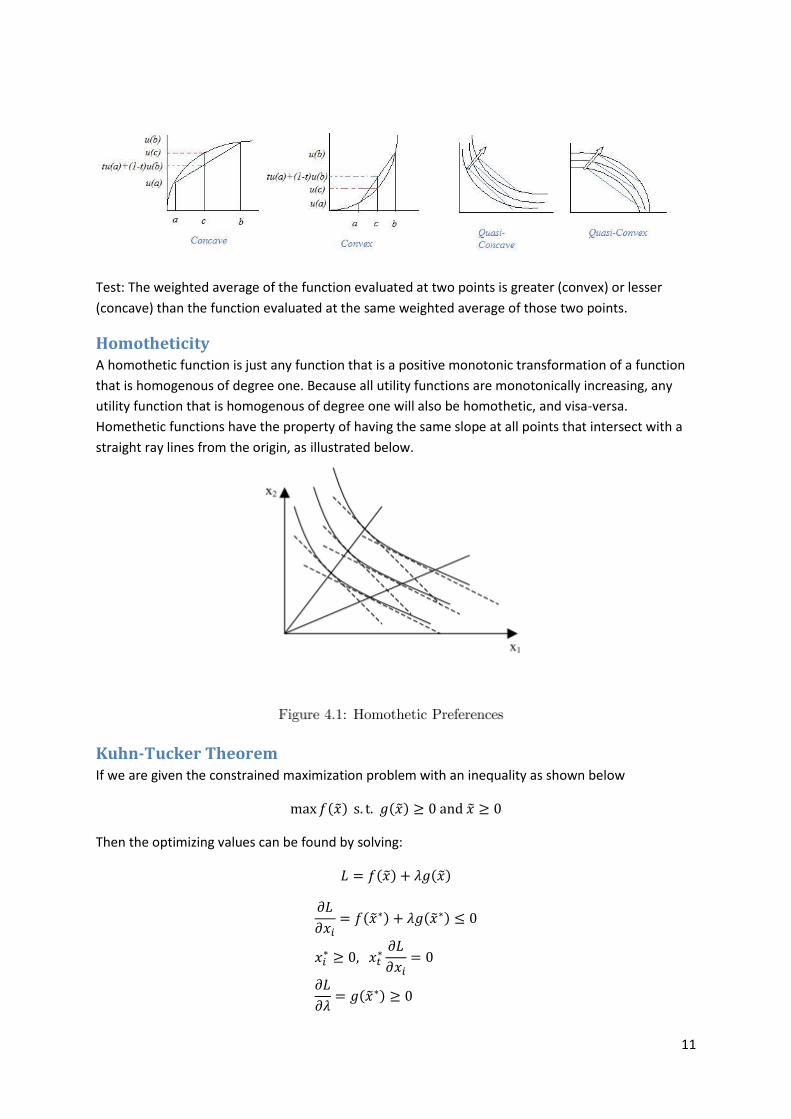
Homotheticity A homothetic function is just any function that is a positive monotonic transformation of a function

that is homogenous of degree one. Because all utility functions are monotonically increasing, any

utility function that is homogenous of degree one will also be homothetic, and visa-versa.

Homethetic functions have the property of having the same slope at all points that intersect with a

straight ray lines from the origin, as illustrated below.

Kuhn-Tucker Theorem If we are given the constrained maximization problem with an inequality as shown below

Then the optimizing values can be found by solving:

12

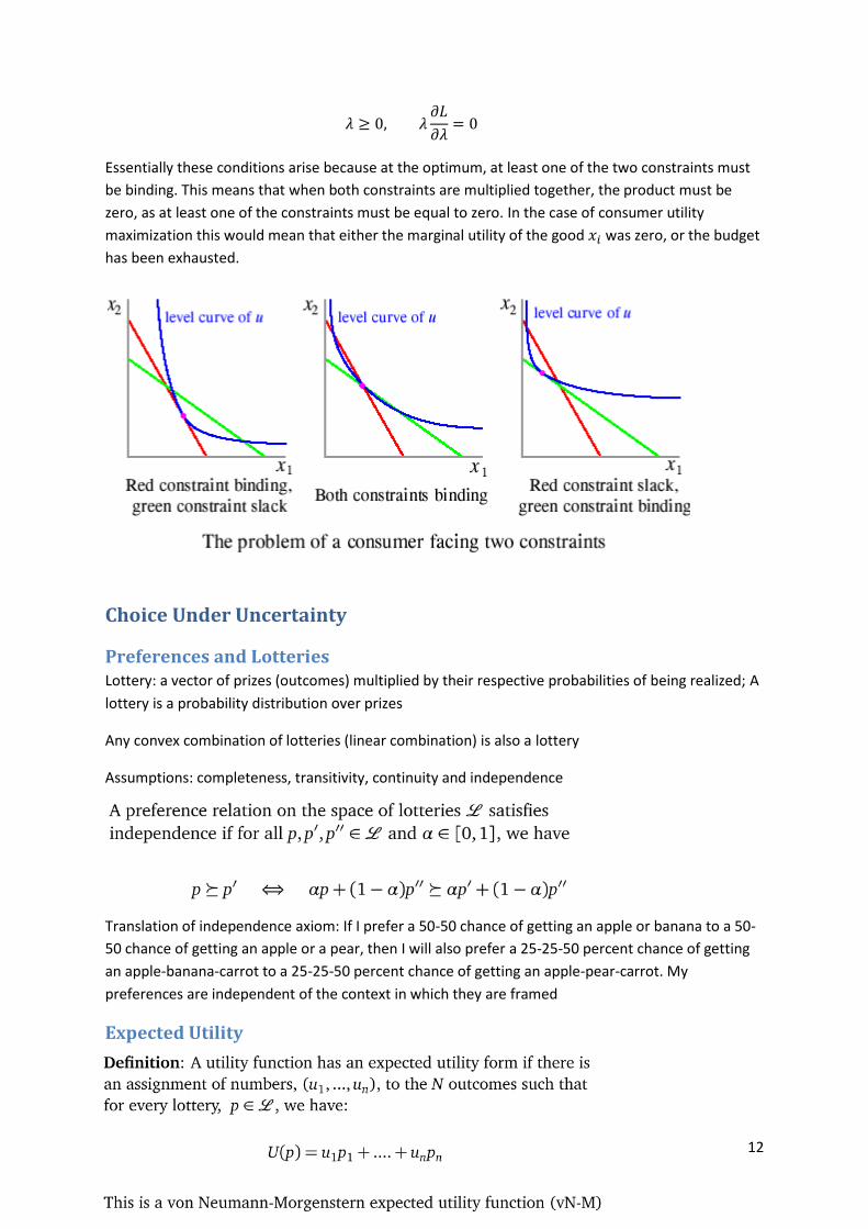
Essentially these conditions arise because at the optimum, at least one of the two constraints must

be binding. This means that when both constraints are multiplied together, the product must be

zero, as at least one of the constraints must be equal to zero. In the case of consumer utility

maximization this would mean that either the marginal utility of the good was zero, or the budget

has been exhausted.

Choice Under Uncertainty

Preferences and Lotteries Lottery: a vector of prizes (outcomes) multiplied by their respective probabilities of being realized; A

lottery is a probability distribution over prizes

Any convex combination of lotteries (linear combination) is also a lottery

Assumptions: completeness, transitivity, continuity and independence

Translation of independence axiom: If I prefer a 50-50 chance of getting an apple or banana to a 50-

50 chance of getting an apple or a pear, then I will also prefer a 25-25-50 percent chance of getting

an apple-banana-carrot to a 25-25-50 percent chance of getting an apple-pear-carrot. My

preferences are independent of the context in which they are framed

Expected Utility

13

Such utility functions are only invariant under positive linear transformations

Expected Utility Theorem: If a preference relation satisfies all four axioms, including that of

independence, then this preference relation can be represented in expected-utility form

VN-M utility functions have linear indifference curves

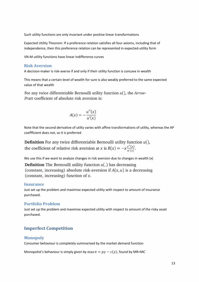
Risk Aversion A decision-maker is risk-averse if and only if their utility function is concave in wealth

This means that a certain level of wealth for sure is also weakly preferred to the same expected

value of that wealth

Note that the second derivative of utilty varies with affine transformations of utility, whereas the AP

coeffficient does not, so it is preferred

We use this if we want to analyze changes in risk aversion due to changes in wealth (x)

Insurance Just set up the problem and maximise expected utility with respect to amount of insurance

purchased.

Portfolio Problem Just set up the problem and maximise expected utility with respect to amount of the risky asset

purchased.

Imperfect Competition

Monopoly Consumer behaviour is completely summarised by the market demand function

Monopolist’s behaviour is simply given by , found by MR=MC

14

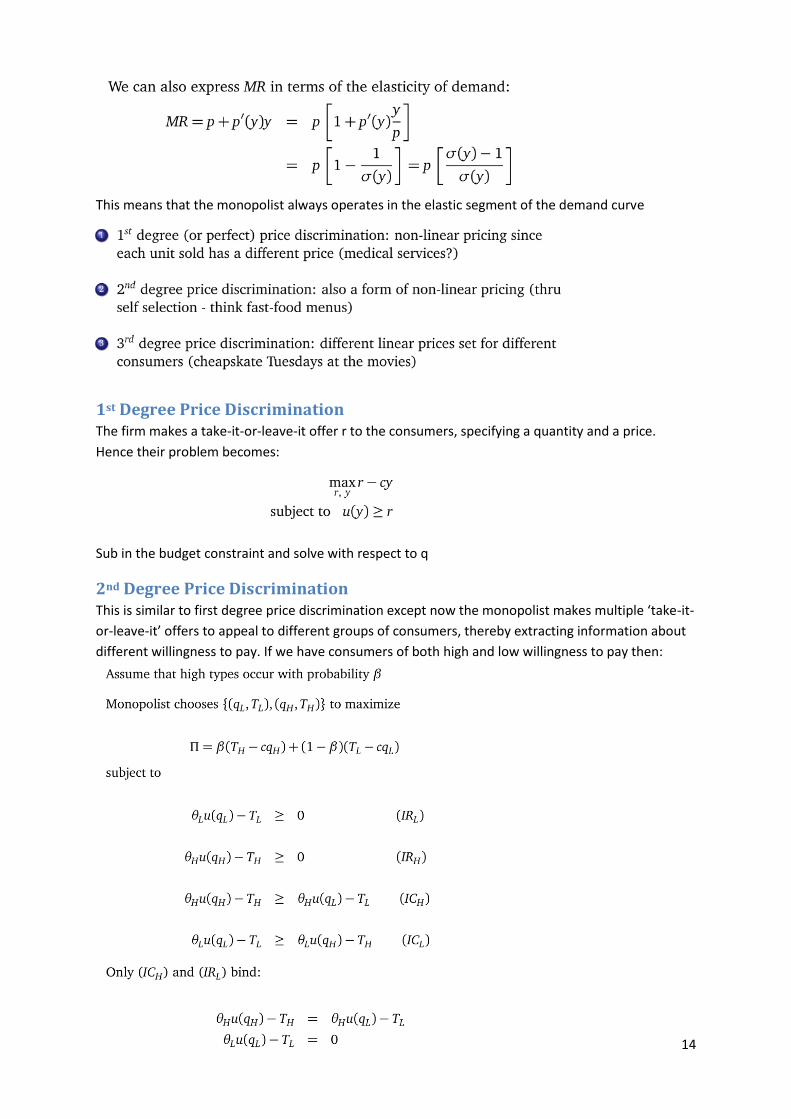
This means that the monopolist always operates in the elastic segment of the demand curve

1st Degree Price Discrimination The firm makes a take-it-or-leave-it offer r to the consumers, specifying a quantity and a price.

Hence their problem becomes:

Sub in the budget constraint and solve with respect to q

2nd Degree Price Discrimination This is similar to first degree price discrimination except now the monopolist makes multiple ‘take-it-

or-leave-it’ offers to appeal to different groups of consumers, thereby extracting information about

different willingness to pay. If we have consumers of both high and low willingness to pay then:

15

Taking these binding constraints, we re-arrange to find prices, and then substitute these into the

objective function, which we can then maximise. Doing so we find that the high-value consumers are

offered the efficient quantity, while the low-value consumers are offered a quantity inefficiently

small.

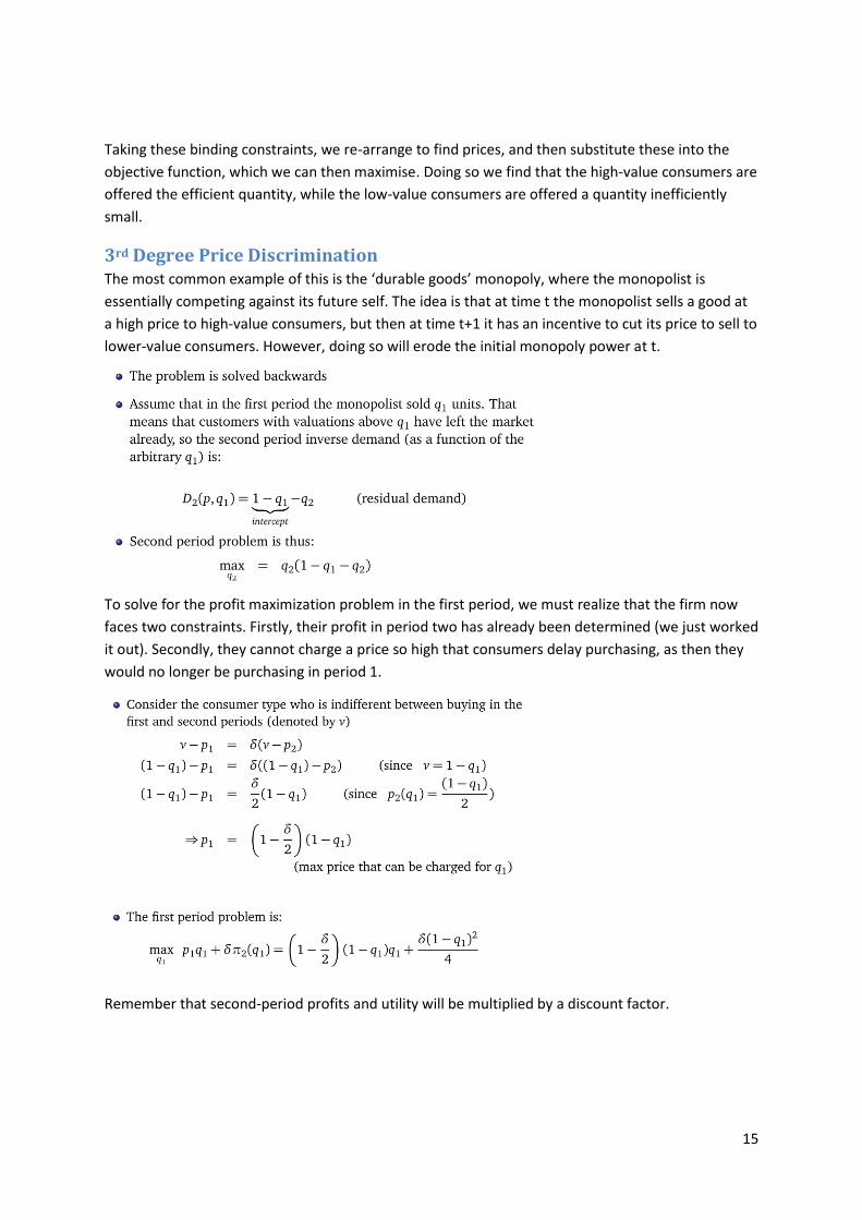
3rd Degree Price Discrimination The most common example of this is the ‘durable goods’ monopoly, where the monopolist is

essentially competing against its future self. The idea is that at time t the monopolist sells a good at

a high price to high-value consumers, but then at time t+1 it has an incentive to cut its price to sell to

lower-value consumers. However, doing so will erode the initial monopoly power at t.

To solve for the profit maximization problem in the first period, we must realize that the firm now

faces two constraints. Firstly, their profit in period two has already been determined (we just worked

it out). Secondly, they cannot charge a price so high that consumers delay purchasing, as then they

would no longer be purchasing in period 1.

Remember that second-period profits and utility will be multiplied by a discount factor.

16

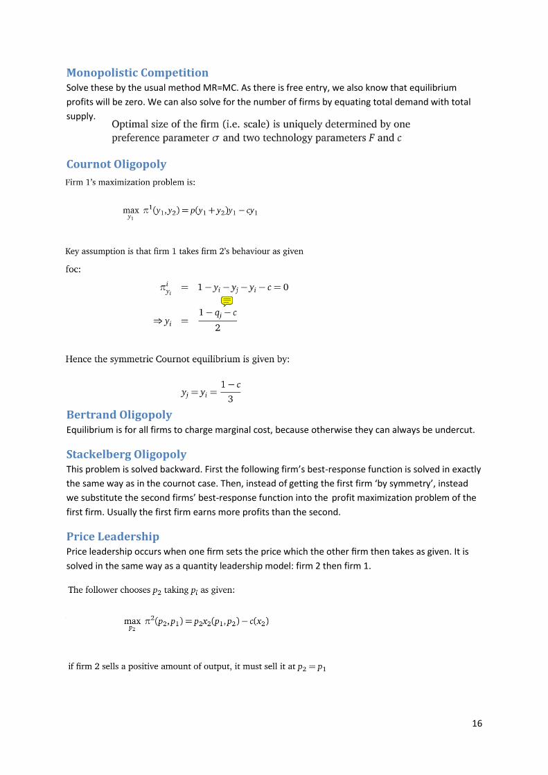
Monopolistic Competition Solve these by the usual method MR=MC. As there is free entry, we also know that equilibrium

profits will be zero. We can also solve for the number of firms by equating total demand with total

supply.

Cournot Oligopoly

Bertrand Oligopoly Equilibrium is for all firms to charge marginal cost, because otherwise they can always be undercut.

Stackelberg Oligopoly This problem is solved backward. First the following firm’s best-response function is solved in exactly

the same way as in the cournot case. Then, instead of getting the first firm ‘by symmetry’, instead

we substitute the second firms’ best-response function into the profit maximization problem of the

first firm. Usually the first firm earns more profits than the second.

Price Leadership Price leadership occurs when one firm sets the price which the other firm then takes as given. It is

solved in the same way as a quantity leadership model: firm 2 then firm 1.

A Model of Sales

Equilibrium Analysis

17

Since price is fixed for firm 2, it suffers no inframarginal loss, and hence will simply supply when

P=MC.

In this case generally both firms prefer to be the follower.

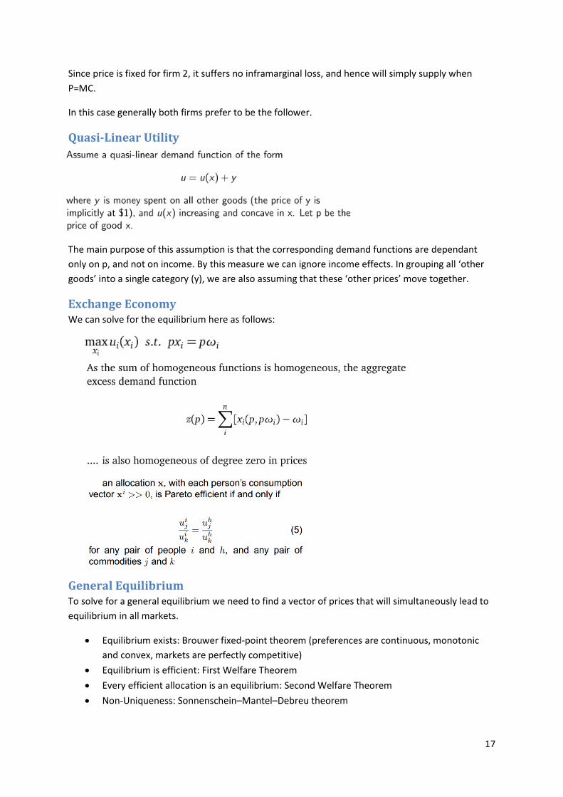
Quasi-Linear Utility

The main purpose of this assumption is that the corresponding demand functions are dependant

only on p, and not on income. By this measure we can ignore income effects. In grouping all ‘other

goods’ into a single category (y), we are also assuming that these ‘other prices’ move together.

Exchange Economy We can solve for the equilibrium here as follows:

General Equilibrium To solve for a general equilibrium we need to find a vector of prices that will simultaneously lead to

equilibrium in all markets.

Equilibrium exists: Brouwer fixed-point theorem (preferences are continuous, monotonic

and convex, markets are perfectly competitive)

Equilibrium is efficient: First Welfare Theorem

Every efficient allocation is an equilibrium: Second Welfare Theorem

Non-Uniqueness: Sonnenschein–Mantel–Debreu theorem

18

Solving a General Equilibrium 1. Use cost-minimisation to solve for factor demands given output (easier to do this by subbing

in constraint) in all final goods markets

2. Rearrange the factor market clearing conditions so that they are in terms of output as a

function of factor demand prices and quantities (subbing in the equations found above)

3. Substitute these modified market clearing equations and the factor demand equations into

the production functions, which should now give good supply as a function of K, L, w and r

4. Solve consumer’s utility maximization problem to find marshallian demand functions

5. Substitute that zero profit condition (which gives prices in terms of cost) and the budget

constraint into the Marshallian demand functions

6. Equate demand and supply in each market, and solve for factor and output prices

7. Substitute these back into production functions to solve for output

Exam Notes To prove all goods can’t be inferior, just differentiate the budget constraint

Remember Gorman form:

When firm has two production technologies, solve for cost function separately and then take

min of these

Concave utility -> quasiconcave utility -> convex level curves (indifference curves) -> convex

preferences

In an endowment economy, the consumer effectively has two budget constraints (in terms

of endowments and in terms of spending)

For price-leadership, you know the second firm will set P=MC. Hence find their quantity that

corresponds to this, and sub this into the leader’s demand to profit maximise

Kuhn-Tucker: write out lagrangian and find all four FOC, treat first two as equalities and

rearrange to get x’s in terms of lambdas, take lambda times budget constraints equate to

zero and solve for lambda, try different solutions (picking one from each condition)

Cournot oligopoly: find the policy reaction function for each firm by profit maximization,

then just solve the resulting system of simultaneous equations

Stackelberg oligopoly: find firm 2’s policy reaction function and sub it into firm 1’s profit

maximization equation before differentiating

Pareto efficiency occurs when consumers have equal MRS

Homothetic preferences are a subset of Gorman Polar Form preferences. You need GPF

preferences to get a unique GE

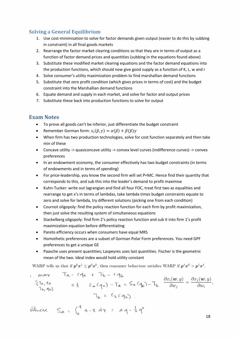
Paasche uses present quantities; Laspeyres uses last quantities. Fischer is the geometric

mean of the two. Ideal index would hold utility constant