Embed Size (px)
Citation preview
Version 08.04.2016
Advanced Lab Course
MOKE Microscopy M209
Stand: 2016-04-08
Aim: Characterization of magnetization reversal of magnetic bulk and thin film samples by means of magneto-optical Kerr effect and recording of magnetic domain patterns of extended and patterned magnetic materials by Kerr microscopy. Contents:
1 Introduction 1
2 Basics 1 2.1 Ferromagnetic hysteresis 1 2.2 Magnetic domains 2 2.3 Magneto-optical Kerr effect microscopy 4 2.4 Equipment – the MOKE microscope 7 2.5 Electrical steel 7 2.6 Amorphous thin films 8
3 Experiments 9 3.1 Kerr microscope 9 3.2 Analysis of magnetic switching behavior and domains of FeCoBSi thin films 9 3.3 Investigation of influence of patterning on reversal in thin film samples 9 3.4 Investigation of the magnetic domain patterns on electrical steel 9
4 Analysis 10 4.1 Alignment of Kerr contrast in the microscope 10 4.2 Magnetic properties of a FeCoBSi film sample 10 4.3 Magnetic properties and magnetic domains of the patterned FeCoBSi film sample 10 4.4 Magnetic domains of electrical steel 10 4.5 Best image 10
5 References 11
M209: MOKE Microscopy
1
1 Introduction
Kerr microscopy is one of the most versatile techniques to image magnetic domains and
magnetization processes. The method is based on the magneto-optical Kerr effect (MOKE),
i.e. the rotation of plane polarized light in dependence of the magnetization direction on
reflection from a non-transparent sample. By this an image of the magnetization distribution
of the surface can be recorded. Moreover, magnetic hysteresis curves can be recorded.
2 Basics
2.1 Ferromagnetic hysteresis
The suitability of ferromagnetic materials for particular applications is determined largely
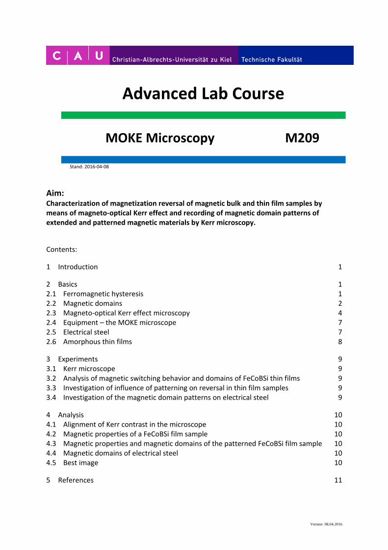
from characteristics shown by their hysteresis loops. Figure 1 displays a typical hysteresis
loop as expected for measuring the magnetization M as a function of the applied magnetic
field H for a ferromagnetic sample.
Fig. 1 Hysteresis loop of a ferromagnetic sample showing the saturation magnetization MS, the remanent magnetization Mr and the coercive field Hc. The applied field H and the plotted magnetization component M are collinear.
The sample is magnetized to the saturation magnetization MS by a strong enough applied
magnetic field. When the applied saturation field is then reduced to zero, the magnetization
decreases to the remanent magnetization Mr. The reversed field required to reduce the
M209: MOKE Microscopy
2
magnetization to zero is called the coercivity or coercive field Hc. The parameters Mr and Hc
can be used to characterize a ferromagnet.
The energy dissipated by a ferromagnet as it is taken around a circuit of its hysteresis loop is
proportional to the area of the hysteresis loop. If the area is small, the material is said to be
magnetically soft.
2.2 Magnetic domains
In general a non-saturated ferromagnet contains a number of small regions called magnetic
domains, where the local magnetization is homogeneous and reaches the saturation value. The
formation of domains allows a ferromagnetic material to minimize its total magnetic energy,
whereby the magnetostatic energy is the principal driving force for domain formation.
The direction of the magnetization of different domains does not need to be parallel. A
demagnetized sample consists of domains, each ferromagnetically ordered with a vanishing
total magnetization. The boundaries between adjacent domains are called domain walls. In
such domain walls the magnetization rotates continuously.
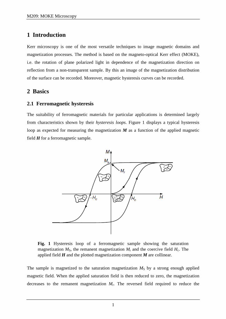
A classification of domain walls can be given by the angle of the magnetization between two
adjacent domains with the wall as boundary. The energetically most favorable types of
domain walls are those which do not produce magnetic poles within the material, and
therefore do not introduce demagnetizing fields. A 180° domain wall represents the boundary
between two domains with oppositely aligned directions of magnetization (Fig. 2a). Here the
magnetization perpendicular to the boundary does not change across the wall and therefore no
magnetic poles or demagnetizing fields arise. Also stable are 90° tilt boundaries (Fig. 2b),
representing the boundary between two domains with magnetization aligned perpendicular to
each other.
Fig. 2 (a) 180° domain wall and (b) 90° domain wall. The directions of magnetization in the adjacent magnetic domains are indicated by arrows.

M209: MOKE Microscopy
3
Fig. 3 (a) A common type of 180° domain wall in bulk materials is a Bloch wall, in which the magnetization rotates in a plane parallel to the plane of the wall. (b) In thin films another possible configuration is the Néel wall, in which the magnetization rotates in a plane perpendicular to the plane of the wall in order to reduce magnetic surface charges and thereby avoiding energetically unfavorable stray fields.
In order to explain the magnetic domain behavior of ferromagnetic samples one has to
consider the total free energy:
( )3
2 2 2 203sin cos2 2
sample
tot u S SV R
dV A grad K dV mφ l s θ = − ⋅ − − + ∫ ∫E M H M H
In the above equation only the energy terms are included relevant for the soft magnetic
samples investigated. The first term, the exchange energy reflects the fundamental property of
a ferromagnet, which favors a constant equilibrium magnetization direction. Deviations from
this homogenous magnetization invoke an energy penalty, the dependency of which can be
described by the gradient of the magnetization. The second term is called the Zeeman energy.
It describes the interaction of the magnetization with an external magnetic field H. It is
minimal for a parallel alignment of magnetization and magnetic field. The energy of a
ferromagnet in most cases also depends on the direction of the magnetization relative to a
certain axis of the material. This dependence is specified by the magnetic anisotropy energy.
The third term of equation describes the uniaxial case of anisotropy, in which the
magnetization lies preferably parallel or anti-parallel to a single easy axis. Ku is the uniaxial
energy density.
An easy axis of magnetization can also be introduced by straining a magnetic body. For
isotropic material and a uniaxial stress σ, the magneto-elastic coupling energy becomes the
fourth term of equation. The material parameter λS is the saturation magnetostriction.
The last term takes the magnetic stray field energy into account, which is connected with the
magnetic stray field Hs generated by the magnetic sample itself. Sinks and sources of the stray
field are “magnetic charges”, which arise for instance when the magnetization has
components perpendicular to the sample’s edge. The stray field energy in magnetic bodies can
be reduced by forming smaller magnetic domains up to the point where further reduction is

M209: MOKE Microscopy
4
balanced by the increase of domain wall energy (Fig. 4). A detailed discussion of the
energetic contributions that determine the magnetization distribution of a ferromagnet is given
in [1].
Fig. 4 Stray field energy Es for a cubic sample with different numbers N of domains. The creation of domain walls reduces the stray field energy Es, but increases the domain wall energy Edw.
2.3 Magneto-optical Kerr effect microscopy
Domain observation by magneto-optics is based on a weak dependence of optical constants on
the direction of magnetization M. The magneto optical Kerr effect is the rotation of the plane
of polarization of a light beam during reflection from a magnetized sample. For most
materials the amount of rotation is very small and depends on both the direction and the
magnitude of the magnetization. It may be applied to the characterization of any metallic or
otherwise light-absorbing magnetic material with a sufficiently smooth surface. The Kerr
effect can be rigorously derived from Maxwell’s equations and proper boundary conditions.
The origin of the magneto-optical effects lies in Zeeman exchange splitting together with
spin-orbit interaction. The symmetry of interaction of a plane-polarized electromagnetic light
wave with a magnetic material can be understood assuming a Lorentz force on moving
electrons initiated by the electrical vector E of the wave (this is not the underlying physical
mechanism).
The occurring change of polarization is sketched in Fig. 5a for the so-called longitudinal Kerr
effect. It generates a magnetic contribution to the reflected light amplitude, the so-called Kerr
amplitude K, which is polarized perpendicularly to the normally reflected amplitude N and
causes rotation of the light through interference with N. In the Kerr microscope for domains
with opposite magnetization, a domain contrast is produced if most of the reflected light of
one domain type is blocked by an analyzer (Fig. 5b). If a noticeable phase shift occurs
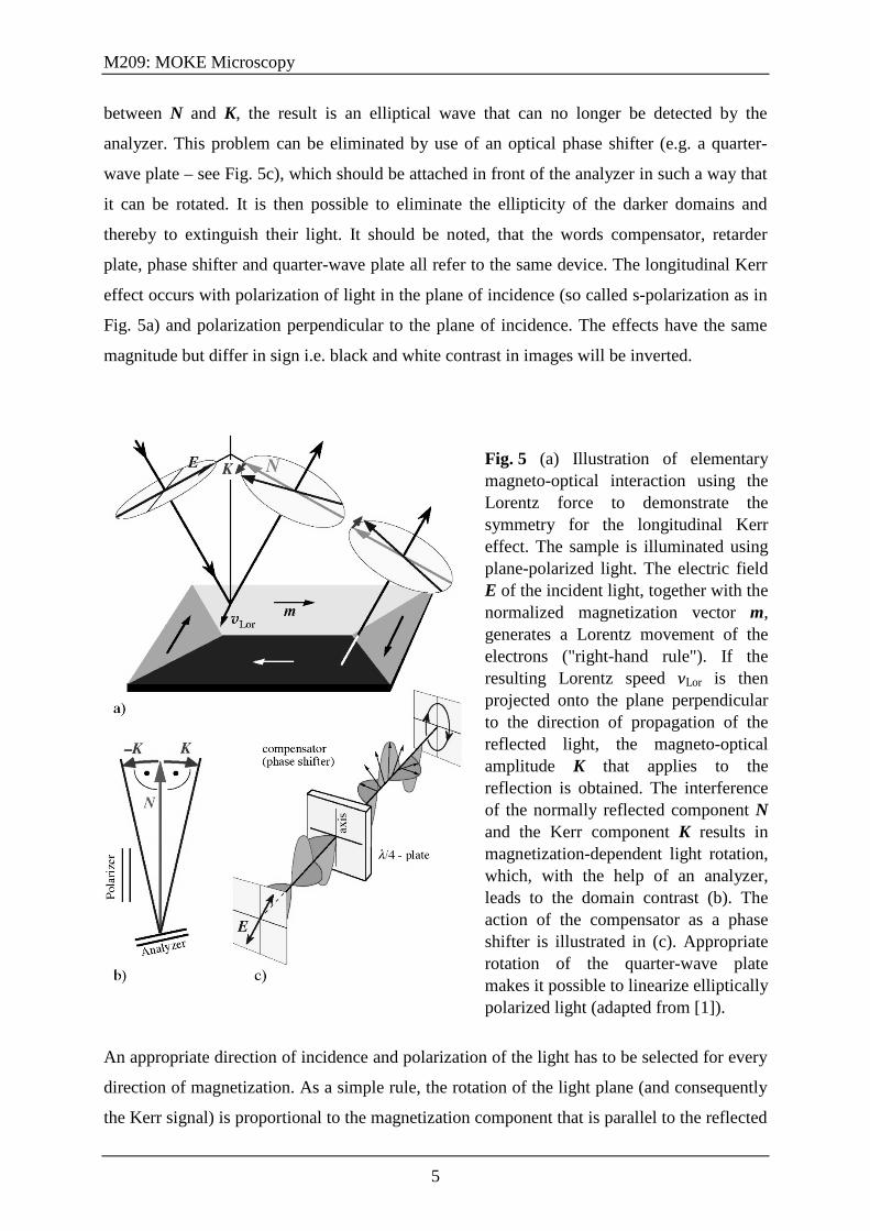
M209: MOKE Microscopy
5
between N and K, the result is an elliptical wave that can no longer be detected by the
analyzer. This problem can be eliminated by use of an optical phase shifter (e.g. a quarter-
wave plate – see Fig. 5c), which should be attached in front of the analyzer in such a way that
it can be rotated. It is then possible to eliminate the ellipticity of the darker domains and
thereby to extinguish their light. It should be noted, that the words compensator, retarder
plate, phase shifter and quarter-wave plate all refer to the same device. The longitudinal Kerr
effect occurs with polarization of light in the plane of incidence (so called s-polarization as in
Fig. 5a) and polarization perpendicular to the plane of incidence. The effects have the same
magnitude but differ in sign i.e. black and white contrast in images will be inverted.
Fig. 5 (a) Illustration of elementary magneto-optical interaction using the Lorentz force to demonstrate the symmetry for the longitudinal Kerr effect. The sample is illuminated using plane-polarized light. The electric field E of the incident light, together with the normalized magnetization vector m, generates a Lorentz movement of the electrons ("right-hand rule"). If the resulting Lorentz speed vLor is then projected onto the plane perpendicular to the direction of propagation of the reflected light, the magneto-optical amplitude K that applies to the reflection is obtained. The interference of the normally reflected component N and the Kerr component K results in magnetization-dependent light rotation, which, with the help of an analyzer, leads to the domain contrast (b). The action of the compensator as a phase shifter is illustrated in (c). Appropriate rotation of the quarter-wave plate makes it possible to linearize elliptically polarized light (adapted from [1]).
An appropriate direction of incidence and polarization of the light has to be selected for every
direction of magnetization. As a simple rule, the rotation of the light plane (and consequently
the Kerr signal) is proportional to the magnetization component that is parallel to the reflected

M209: MOKE Microscopy
6
beam of light. This rule implies that magnetic domains which are magnetized parallel to the
sample surface require oblique light incidence and for maximum contrast the incidence plane
of the light must be parallel to the direction of magnetization (longitudinal Kerr effect). The
longitudinal Kerr signal vanishes for perpendicular incidence. On the other hand, in the case
of perpendicular light incidence maximum contrast is exhibited by domains that are
magnetized perpendicularly to the sample surface (polar Kerr effect).
The main components of a two principle different types of Kerr microscopes are represented
schematically in Fig. 6. As the Kerr effect is weak, a highly intensive light source is used, for
instance a high power LED.
Fig. 6 Symmetrical ray diagram of a Kerr imaging setup for high resolution magnetic domain observations in reflection. (a) Optical path of illumination and (b) simplified path of observation (only the primary image plane is shown). Köhler-type illumination of the specimen is realized by a high power fiber coupled LED light source. Two sets of rays corresponding to two different points in the conjugate sets of aperture planes (AP) are sketched. The locations of rotatable polarizer, retarder plate, and analyzer are shown. The corresponding conjugate sets of field or image planes (IP) are indicated. The image of the AP obtained from a conoscopic image of the back-focal (Fourier) optical plane of the objective lens with insertion of a Bertrand lens in the optical path is shown. (c) Optical ray diagram of a large view magneto-optical Kerr microscope (from [2]).
The domain contrast is optimized by the rotation of analyzer and compensator. For the high
resolution Kerr microscope setup the position of the LED fiber output, controlling the
illumination, has to be adjusted so that angle and plane of incidence can be chosen, allowing
to optimize the Kerr sensitivity to in- or out-of-plane magnetization configurations. The
application of magnetic fields is possible using an electromagnet.
M209: MOKE Microscopy
7
2.4 Equipment – the MOKE microscope
The Kerr microscope consists of the following components: a polarization microscope, a
control computer, an optical table with vibration isolation, an electromagnet, and a sample
stage. A significant enhancement of magnetic contrast is achieved by digital image
processing. The standard procedure starts with a digitized image of the magnetically
homogenous state, where in an external ac or dc magnetic field all domains are eliminated.
This background (reference) image is subtracted from a state containing domain information.
Non-magnetic contrasts, which do not change, are subtracted during this process. So in the
difference image a clear micrograph of the domain pattern is obtained, which can digitally be
enhanced free of topographic structures. This subtraction process is best carried out in real
time at least video frequency, making it possible to view magnetization processes while
retaining the same reference image.
The same effects that are used for imaging can also be used for the general magnetic
characterization of the material, i.e. local magnetic hysteresis curves may be obtained by just
plotting the average intensity of the Kerr images as a function of applied field.
2.5 Electrical steel
The control of the magnetic reversal in soft magnetic bulk materials is essential for improving
their energy efficiency. Electrical steel is a soft magnetic polycrystalline metallic alloy that is
used as a core material in electrical transformer cores. For grain-oriented electrical steels the
reduction in core losses in recent years are due to two major technological advances,
improved texture control and the control of the magnetic domain structure.
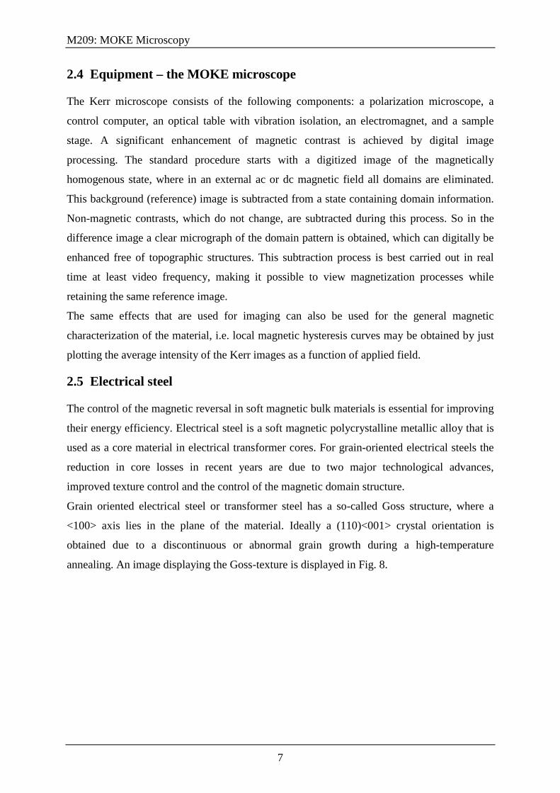
Grain oriented electrical steel or transformer steel has a so-called Goss structure, where a
<100> axis lies in the plane of the material. Ideally a (110)<001> crystal orientation is
obtained due to a discontinuous or abnormal grain growth during a high-temperature
annealing. An image displaying the Goss-texture is displayed in Fig. 8.
M209: MOKE Microscopy
8
Fig. 8: Goss texture. The <100>-axes are the easy axes of magnetization.
Magnetic domain observations deliver the scientific fundaments to understand the important
issues of nucleation and annihilation of surface closure domains and pinning processes in the
movement of 180° domain walls and their interaction with defects like grain boundaries.
2.6 Amorphous thin films
Magnetic amorphous alloys obtained by rapid quenching of the melt or by means of
sputtering are excellent soft magnetic materials with a wide range of technological
applications. Despite the absence of a crystalline structure, amorphous materials can possess a
(uniaxial) magnetic anisotropy. The most common compositions for soft magnetic
applications are metal-metalloid based (Fe, Co, Ni)-(Si,B) alloys with a metalloid contents of
about 20%.
M209: MOKE Microscopy
9
3 Experiments For documentation and for later evaluation store the obtained magnetic hysteresis curves and
images of domain patterns that you have recorded. The experiments will be performed under
supervision. Do not try to operate the Kerr microscope without being first instructed by the
supervisor.
3.1 Kerr microscopes Identify the optical elements as sketched in Fig. 6 at the microscopes. Which elements are
arranged differently?
3.2 Analysis of magnetic switching behavior and domains of FeCoBSi thin films The aim of the investigation is to characterize the magnetic switching behavior of an extended
amorphous FeCoBSi thin film sample. Therefore hysteresis curves are recorded along the
easy axis of magnetization and along the hard axis of magnetization. Obtain typical domain
images at remanent state saturating the samples along and perpendicular to the easy axis of
magnetization.
3.3 Investigation of influence of patterning on reversal in thin film samples The aim of this part is to investigate the switching behavior of FeCoBSi thin film structure.
Record the magnetization loops along both perpendicular edges of the square elements.
Identify the easy axis of magnetization in the patterned sample. Obtain typical domain images
after demagnetization of the sample along and perpendicular to the easy axis of
magnetization. Obtain typical domain images at remanent state saturating the samples along
and perpendicular to the easy axis of magnetization. Compare the obtained magnetic domain
patterns.
3.4 Investigation of the magnetic domain patterns on electrical steel The aim of the investigation is to characterize the different domain patterns in SiFe. Obtain
typical surface domain images after demagnetization of the sample along and perpendicular to
the easy axis of magnetization. Can you identify different grains? How are the domain
patterns changing with the application of a magnetic field along the easy axis and hard axis of
magnetization?

M209: MOKE Microscopy
10
4 Analysis 4.1 Alignment of Kerr contrast in the microscope Describe the necessary steps in order to achieve longitudinal Kerr contrast in the Kerr
microscopes. How many ways are to obtain longitudinal contrast in the microscopes?
4.2 Magnetic properties of a FeCoBSi film sample Describe the switching behavior in terms of remanent magnetization, coercive field and
saturation field. Is there any hint for a magnetic anisotropy?
4.3 Magnetic properties and magnetic domains of the patterned FeCoBSi film sample Describe the observed domain patterns in terms of domain width and preferential
magnetization directions. Is there any dependency of the magnetic domain width on the
magnetic history? How does the hysteresis loop change with patterning and direction of field
(compare to the non-structured sample)?
4.4 Magnetic domains of electrical steel Describe typical domain patterns obtained at the surface of the electrical steel sheet. What
does it tell you about the crystallographic orientation of the iron sheet? Discuss how the
surface domain patterns obtained with and without the application of a magnetic field
correlate to the bulk domain structure. Is the magnetic flux propagating across the grain
boundaries?
4.5 Best image Which is in your view the nicest domain image that you took? Why?
M209: MOKE Microscopy
11
5 References [1] A. Hubert, R. Schäfer, Magnetic Domains, Springer-Verlag Berlin, Heidelberg, 1998
[2] J. McCord, Progress in magnetic domain observation by advanced magneto-optical
microscopy, Journal of Physics D: Applied Physics 48, 333001 (2015)
[3] http://magnetism.eu/esm/2005-constanta/abs/mccord-abs.pdf
[4] http://magnetism.eu/esm/2005-constanta/slides/mccord-slides.pdf
[5] N. Spaldin, Magnetic Materials – Fundamentals and applications, Cambridge, 2003