Data being collected by the Mars Global Surveyor (MGS)are providing a fascinating and unexpected image of the mag-netic field of Mars. Early results from Mario Acuña, principalinvestigator of the magnetometer experiment, and his cowork-ers from NASA’s Goddard Space Flight Center showed mag-netic stripes over parts of the southern hemisphere evocativeof those in the ocean basins on Earth that are caused by themagnetization of new crust generated at spreading ridges inan alternating polarity field. This suggests that plate tecton-ics may have occurred on Mars, and implies that the Martiandynamo reversed during its short life, which must have encom-passed the creation of new crust. Another pointer to tectonicactivity or at least structural events is the truncation of mag-netic features over the Valles Marineris and Ganges Chasma.

In this article, we present further suggestions of both mag-netic reversals and tectonic activity on Mars from preliminaryresults of an inversion of MGS data for models of crustal mag-netization. We find patterns of magnetization inclinationsreminiscent of a triple junction, and reversed magnetizationpoles.

One of the first surprises from MGS was the strength ofthe Martian magnetic field. Dynamo action ceased in prob-ably the first 0.5 billion years of the planet’s history, so whatwe observe today is the remanent magnetization generatedduring that period and locked into the crust. During the aero-braking phase of the mission, when MGS was as close as120 km to the surface, fields in excess of 1500 nT were mea-sured. We rarely observe such large anomalous remanentmagnetic fields on Earth even in aeromagnetic surveys a fewhundred meters above the terrestrial surface. At sphericalharmonic degrees beyond 14 or so (wavelengths shorter than~2760 km), where we believe the terrestrial field has a negli-gibly small contribution from geodynamo action, there isabout two orders of magnitude more power in the Martianfield. There are a number of possible explanations for this.Such short-lived dynamo action may have been more ener-getic, generating higher strength magnetizing fields while itwas in operation. There is thought to be more iron in theMartian than terrestrial crust, so we might expect highermagnetizations to result from the same magnetizing fieldstrength. The mineralogy could be different, again poten-tially leading to larger magnetizations. But although theMartian surface, with planetary radius about 3393 km, iscloser to its core (radius between 1520 km and 1840 km) thanin the terrestrial case, the attenuation of the field strengthdepends on the ratio of radii of the planet to its core, not thedistance between them. This ratio is larger for Mars (~2.0)than for Earth (1.8), leading to greater attenuation.

The data inverted to obtain the magnetization models pre-sented here are vertical component magnetic field measure-ments collected in two phases of the mission, at altitudesbetween approximately 100 and 600 km, and provide almostcomplete coverage. Vertical component data are less contam-inated by external magnetic fields (due to solar activity) thanthe horizontal components. To reduce the data scatter and thecomputational effort involved in inversion, and because wecannot resolve features less than 100 km or so (the minimumaltitude at which measurements have been made), the datahave been averaged into 1º bins (1º represents approximately60 km on the Martian surface). We only included bins con-taining more than one data point, giving a statistical measure

of uncertainty. This reduced the data set to 49 635 points. Datawere normalized to unit variance using these standard devi-ations. There are several images in the literature of data setscollected earlier in the mission, such as that by one of us(MEP) and coworkers at Goddard Space Flight Center, onwhich key features referred to here are labeled. Mars showsa large contrast between strong magnetic fields in the south-ern hemisphere and relatively weak fields over most of thenorthern hemisphere. The dichotomy separating the tworegions also divides the planet into a much higher elevation,more heavily cratered, southern hemisphere and a lower, flat-ter northern hemisphere, as seen from the laser altimeter(MOLA) images. The northern hemisphere contains a signif-icant thickness of extrusives and sediments blanketing muchof the surface. These younger rocks were formed after theMartian dynamo switched off, and are therefore nonmag-netic. However, the underlying older rocks must also be lessmagnetic than those in the southern hemisphere to explainthe low field strengths measured.

Our inversion method solves for a continuous distribu-tion of magnetization within a layer of constant, specifiedthickness (40 km, based on estimates of crustal thickness fromvariations in the topography and gravity field). Inversions ofterrestrial satellite data have indicated that the effect of vary-ing the thickness is that the model magnetizations adjust suchthat the vertically integrated magnetization is constant. Thisis what we would expect—satellites “see” the magnetizedcrust as a thin layer and are unable to resolve depth varia-tions. We feel compelled to remind the reader about the usualambiguities that exist when dealing with specific modelingproblems like these. In this case, unique solutions are obtainedby requiring that our models have minimum average mag-netization strength, for a given fit to the data.

Within this framework, we solve for the model coeffi-cients, a daunting computational task, because the designmatrix relating them to the data has almost 2.5 billion elements!Fortunately, most elements are negligibly small, and we cantherefore regard it as numerically sparse. Based on previous

AUGUST 2003 THE LEADING EDGE 763

Martian magnetization—preliminary modelsK. A. WHALER, University of Edinburgh, ScotlandM. E. PURUCKER, Raytheon ITSS at Geodynamics Branch, NASA/GSFC, Maryland, U.S.

Figure 1. Globalmaps (Hammerprojection) of a mag-netization model forMars produced byour method. Thenorth (X), east (Y)and vertically down-ward (Z) componentsof magnetization arein A/m (color scale).Note the contrastbetween the weaklymagnetized area tothe north of thedichotomy (solidline) and the morestrongly magnetizedarea to its south. Thecentral meridian is180º longitude.

studies, we retained the largest 0.87% (approximately 21 mil-lion) elements of the design matrix, treating the remainder asif they were zero, and used the iterative conjugate gradientalgorithm to determine the model coefficients.

The relative importance of fitting the data and minimiz-ing magnetization strength is controlled by a damping para-meter. There is a direct analogy between models produced byour method and damped equivalent source magnetizationmodels: Both have minimum average magnetization strength.Equivalent sources is a common way to produce magnetiza-tion models: The volume of crust to be modeled is dividedinto blocks, with a magnetic dipole at the center of each.Usually, the directions in which the dipoles point are speci-fied, leaving their strengths to be deduced from the data.Magnetization is then deduced by normalizing by the volumeof the block.

Figure 1 is an example magnetization model calculatedusing our method. The north (X), east (Y) and vertically down-ward (Z) components are plotted. Note that we infer the fullmagnetization vector, although only vertical component mag-netic field data were inverted. In our models, vertical com-ponent magnetization is highest, but there is significant powerin the horizontal components. Figure 1 shows a strong mag-netization contrast across the dichotomy. North of thedichotomy, magnetic features are relatively isolated, and wecan see a direct association between features of the magneti-zation model and features in the original data. South of thedichotomy, the magnetic field is significant almost every-where, and is modeled as continuous, strong magnetization.A puzzling feature of our model is the large magnetization inall three components over the North Pole. The data plots showonly slightly enhanced amplitudes in this region, which maybe caused partly by external field contamination. Future stud-ies will investigate this region further. However, the modelselsewhere look to be a good representation of the data. Wehave also compared the vertical component of our models withvertical dipole equivalent source models, and agreement isencouraging.

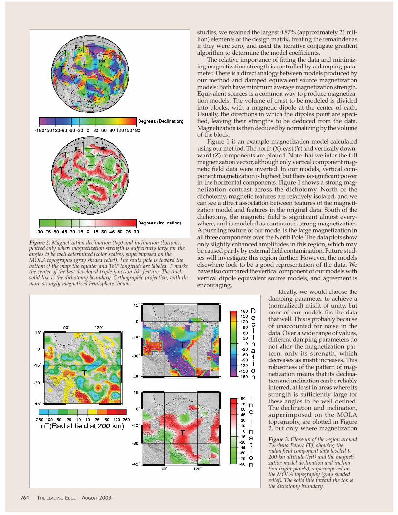
Ideally, we would choose thedamping parameter to achieve a(normalized) misfit of unity, butnone of our models fits the datathat well. This is probably becauseof unaccounted for noise in thedata. Over a wide range of values,different damping parameters donot alter the magnetization pat-tern, only its strength, whichdecreases as misfit increases. Thisrobustness of the pattern of mag-netization means that its declina-tion and inclination can be reliablyinferred, at least in areas where itsstrength is sufficiently large forthese angles to be well defined.The declination and inclination,superimposed on the MOLAtopography, are plotted in Figure2, but only where magnetization

764 THE LEADING EDGE AUGUST 2003

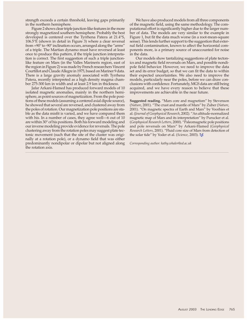
Figure 3. Close-up of the region aroundTyrrhena Patera (T), showing theradial field component data leveled to200-km altitude (left) and the magneti-zation model declination and inclina-tion (right panels), superimposed onthe MOLA topography (gray shadedrelief). The solid line toward the top isthe dichotomy boundary.

Figure 2. Magnetization declination (top) and inclination (bottom),plotted only where magnetization strength is sufficiently large for theangles to be well determined (color scales), superimposed on theMOLA topography (gray shaded relief). The south pole is toward thebottom of the map; the equator and 180º longitude are labeled. T marksthe center of the best developed triple junction-like feature. The thicksolid line is the dichotomy boundary. Orthographic projection, with themore strongly magnetized hemisphere shown.

strength exceeds a certain threshold, leaving gaps primarilyin the northern hemisphere.

Figure 2 shows clear triple junction-like features in the morestrongly magnetized southern hemisphere. Probably the bestdeveloped is centered over the Tyrrhena Patera at 21.4°S,106.5°E (shown in detail in Figure 3) where a clear reversalfrom +90° to -90° inclination occurs, arranged along the “arms”of a triple. The Martian dynamo must have reversed at leastonce to produce this pattern, if the triple junction interpreta-tion is correct. The first suggestion of such a triple junction-like feature on Mars (in the Valles Marineris region, east ofthe region in Figure 2) was made by French researchers VincentCourtillot and Claude Allegre in 1975, based on Mariner 9 data.There is a large gravity anomaly associated with TyrrhenaPatera, recently interpreted as a high density magma cham-ber 275-300 km in width and at least 2.9 km in thickness.

Jafar Arkani-Hamed has produced forward models of 10isolated magnetic anomalies, mainly in the northern hemi-sphere, as point sources of magnetization. From the pole posi-tions of these models (assuming a centered axial dipole source),he showed that several are reversed, and clustered away fromthe poles of rotation. Our magnetization pole positions are sta-ble as the data misfit is varied, and we have compared themwith his. In a number of cases, they agree well—6 out of 10are within 30° of his positions. Both his forward modeling andour inverse modeling provide evidence for reversals. The poleclustering away from the rotation poles may suggest plate tec-tonic movement (such that the site of the cluster was origi-nally at a rotation pole), or a dynamo field that was eitherpredominantly nondipolar or dipolar but not aligned alongthe rotation axis.

We have also produced models from all three componentsof the magnetic field, using the same methodology. The com-putational effort is significantly higher due to the larger num-ber of data. The models are very similar to the example inFigure 1, but fit the data much worse (in a root-mean-squaresense). This lends further support to the suggestion that exter-nal field contamination, known to affect the horizontal com-ponents more, is a primary source of unaccounted for noisein the data.

Our models show tantalizing suggestions of plate tecton-ics and magnetic field reversals on Mars, and possible nondi-pole field behavior. However, we need to improve the dataset and its error budget, so that we can fit the data to withintheir expected uncertainties. We also need to improve themodels, particularly near the poles, before we can draw con-clusions with confidence. Fortunately, MGS data are still beingacquired, and we have every reason to believe that theseimprovements are achievable in the near future.

Suggested reading. “Mars core and magnetism” by Stevenson(Nature, 2001). “The crust and mantle of Mars” by Zuber (Nature,2001). “On magnetic spectra of Earth and Mars” by Voorhies etal. (Journal of Geophysical Research, 2002). “An altitude-normalizedmagnetic map of Mars and its interpretation” by Purucker et al.(Geophysical Research Letters, 2000). “Paleomagnetic pole positionsand pole reversals on Mars” by Arkani-Hamed (GeophysicalResearch Letters, 2001). “Fluid core size of Mars from detection ofthe solar tide” by Yoder et al. (Science, 2003). TLE

Corresponding author: kathy.whaler@ed.ac.uk

AUGUST 2003 THE LEADING EDGE 765