ACCEPTED FOR PUBLICATION IN THE AERONAUTICAL JOURNAL

Advanced gas turbine performancemodelling using response surface methods

Vaishnavi Seetharama-Yadiyal, Giovanni David Brighenti and Pavlos K Zachos

p.zachos@cranfield.ac.uk

Propulsion Engineering Centre, Cranfield University, MK43 0AL, Cranfield, United Kingdom

ABSTRACT

Surrogate models are widely used for dataset correlation. A popular application very frequently shown in publicliterature is in the field of engineering design where a large number of design parameters is correlated withperformance indices of a complex system based on existing numerical or experimental information. Such anapproach allows the identification of the key design parameters and their impact on the system’s performance.The generated surrogate model can become part of wider computational platforms and enable optimisation of thecomplex system without the need to run expensive simulations.

In this paper a number of design point simulations for a combined gas-steam cycle are used to generate a responsesurface. The generated response surface correlates a range of cycle’s key design parameters with its thermalefficiency while it also enables identification of the optimum overall pressure ratio and the high pressure level ofthe raised steam across a range of recuperator effectiveness, pinch temperature difference across the heat recoverysteam generator and the pressure at the condenser. The accuracy of a range of surrogate models to capture thedesign space is evaluated using root mean square statistical metrics.

Keywords: Surrogate modelling, response surface, combined cycle gas turbines

NOMENCLATURE

CCGT Combined Cycle Gas Turbine

HP High PressureHRSG Heat Recovery Steam GeneratorLP Low PressureOPR Overall Pressure RatioPRESS RMSE Predicted Sum of Square RMSEREC RecuperatorRMSE Root Mean Square ErrorRSM Response Surface MethodSBC Steam bottoming cycleTIT Turbine Inlet Temperature, KTERA Techno-economical Environmental Risk AnalysisMLE Maximum Likelihood Estimation

Symbols

∆THRSG HRSG pinch temperature difference, K

ε Heat exchanger effectiveness

η Efficiency-log L Log LikelihoodX Parameter calculated in the probability analysis

σ Standard deviation

1.0 INTRODUCTION

In evaluating the thermal performance of advanced power cycles, a key aspect is the cycle’s thermal efficiencyacross a defined design space. This enables the assessment of the influence of the key design parameters. Veryfrequently, the complexity of the power plant and the number of thermodynamic design variables make itcomputationally challenging to simulate a sufficient number of cycles for an acceptable representation of itsefficiency across the prescribed design space. In that context response surface approaches can be used toapproximate the cycle’s performance metrics and the correlate key design parameters with the efficiency of thepower system. Such an approach would allow the integration of cycle’s performance within a wider analysis deckthat enables a number of preliminary design and analysis studies as for example integrated power plantperformance, lifecycle economic analysis, noise or emissions such as the ones discussed previously in TERAanalysis in the marine sector [1,2] or in aerospace [3],[4,5] or in power generation [6].

Surrogate models have been used successfully in various fields where computational simulations orexperimentations are time expensive or of difficult realization, for instance and among others: in reservoirengineering for predicting the flow of fluids (typically, oil, water, and gas) through porous media [7], in bio-engineering for the optimization of the relative ratio of three factors influencing cardiomyocyte cell differentiation[8] and in aerospace field to predict the noise levels generated by contra rotating open rotor propellers [4].

This article focuses on the development and application of a Response Surface Method to approximate theefficiency of gas-steam combined cycle power plant at design point across a range of design parameters. A largenumber of cycle performance simulations is used as the underlying dataset for the generation of the responsesurface. A range of statistical and mathematical techniques are herein analysed with regards to their capability tocreate a response surface models, for the thermal efficiency and the free design variables, that links the cycle’sperformance with the variation of free design parameters across a design space for a combined-cycle gas turbines(CCGT).

2.0 GENERATION OF TRAINING DATA SET

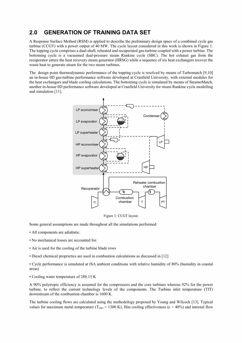
A Response Surface Method (RSM) is applied to describe the preliminary design space of a combined cycle gasturbine (CCGT) with a power output of 40 MW. The cycle layout considered in this work is shown in Figure 1.The topping cycle comprises a dual-shaft, reheated and recuperated gas-turbine coupled with a power turbine. Thebottoming cycle is a vacuumed dual-pressure steam Rankine cycle (SBC). The hot exhaust gas from therecuperator enters the heat recovery steam generator (HRSG) while a sequence of six heat exchangers recover thewaste heat to generate steam for the two steam turbines.

The design point thermodynamic performance of the topping cycle is resolved by means of Turbomatch [9,10]an in-house 0D gas-turbine performance software developed at Cranfield University, with external modules forthe heat exchangers and blade cooling calculations. The bottoming cycle is simulated by means of SteamoMatch,another in-house 0D performance software developed at Cranfield University for steam Rankine cycle modellingand simulation [11].

Figure 1: CCGT layout.

Some general assumptions are made throughout all the simulations performed:

• All components are adiabatic.

• No mechanical losses are accounted for.

• Air is used for the cooling of the turbine blade rows

• Diesel chemical proprieties are used in combustion calculations as discussed in [12]

• Cycle performance is simulated at ISA ambient conditions with relative humidity of 80% (humidity in coastalareas)

• Cooling water temperature of 288.15 K

A 90% polytropic efficiency is assumed for the compressors and the core turbines whereas 92% for the powerturbine, to reflect the current technology levels of the components. The Turbine inlet temperature (TIT)downstream of the combustion chamber is 1600 K.

The turbine cooling flows are calculated using the methodology proposed by Young and Wilcock [13]. Typicalvalues for maximum metal temperature (Tmax = 1300 K), film cooling effectiveness (ε = 40%) and internal flow

cooling efficiency (ηc= 70%) are fixed in agreement with Horlock [14]. The cooling flows for all turbines, ifnecessary, are extracted downstream of the recuperator and upstream of the combustion chamber.

A 90% polytropic efficiency is assumed for the steam power turbines whereas an isentropic efficiency of bothcirculation and service pumps is set at 80% in agreement with current technology limits. The steam quality at theoutlet of the turbines is limited to be higher than 85%, to avoid erosions in the last stages of the turbine due tohigh number of condensate droplets [15].

In the recuperator, the inlet properties of both streams are defined, therefore the outlet conditions of the twostreams are calculated by defining the effectiveness of the heat exchanger (ε= Q/Qmax). The pressure levels of theHRSG —ie. high and low-pressure levels— are resolved by imposing the pinch temperature difference betweenthe steam-water and the gas at the outlet of the superheater and at the inlet of the evaporator. The approachtemperature difference to the evaporator is 2 K to reflect the current technology level in HRSG. The minimumsuper-heater pinch temperature difference is limited to 20 K whereas the maximum steam temperature is limitedto 850 K, a common creep limit for Ni-Cr steels for times of order of 30-40 years [16].

The required steam-water mass flow for the bottoming cycle is calculated by imposing the two pinch temperaturedifferences and resolving the HRSG energy balance system of equations. In the condenser, the inlet and outletconditions and mass flow of the condensing steam are known and temperature difference between the coolant atthe inlet and outlet is imposed to be 5 K. The required coolant mass flow is therefore calculated solving the energybalance in the condenser. The total pressure losses of the heat exchanger are assumed to be 5% in both sides ofall heat exchangers. In the evaporators, the pressure losses are compensated by the circulation pumps and thepower consumption of the latter is accounted for in the cycle thermal efficiency calculations.

The exploration of the cycle design space aims to evaluate the impact of the technology challenges across themain cycle components on the system’s performance. One of the main concerns about the CCGT cycle is theimpact of the total heat transfer area, required to achieve high thermal efficiency. The design space explorationis, therefore, focused on identifying the impact of the technology level of the cycle key heat exchangers —ie.recuperator and HRSG— on its overall thermal efficiency.

The most representative thermodynamic design variable for the technology level of the recuperator is itseffectiveness. The higher the heat exchanger effectiveness, the smaller is the minimum achieved temperaturedifference between the hot and cold streams at the exit which yields to a continuously decreasing heat flux betweenthe two streams as a function of the heat exchanger’s effective length. This reflects in bulkier heat exchangersor/and the need to deploy more expensive materials to increase the heat transfer coefficient within the heatexchangers.

The design parameter that mostly affects the size and weight but also the performance of the HRSG is theevaporator pinch temperature difference (∆THRSG). The amount of heat recovered from the exhaust gas stronglydepends on the latter, but while the steam generated by the HRSG has a linear dependency with the evaporatorpinch point, the heat transfer area of the HRSG varies exponentially further pronouncing the increase in size forlow ∆THRSG. One of the cycle parameters that mostly affects the size and weight of the condenser is the condensingpressure in the Rankine cycle due to the effect it has on the amount of heat that needs to be rejected to liquefy thesteam.

The above-mentioned design variables, representative of the analysed components technology level, are variedparametrically as shown in Table 1 to create a multi-dimensional mesh of the design space for the training of theresponse surface.

Table 1: Ranges for the free design variables of the CCGT design space.

CCGT

Design variable Units Values Steps

Recuperator effectiveness, εREC (-) [0.7 0.95] 8HRSG pinch temperature difference, ∆THRSG (K) [10 50] 8

Condenser pressure, PCND (kPa) [5 6.5] 8

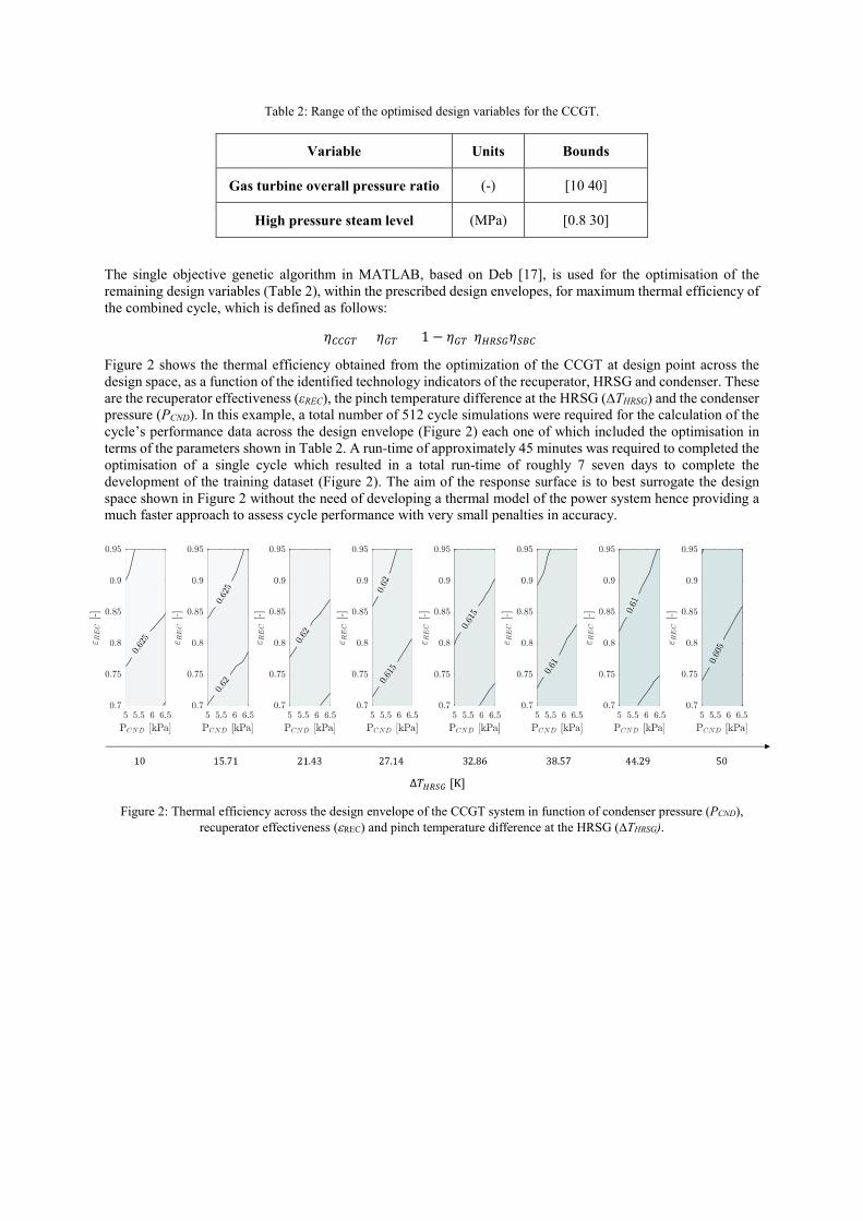
Table 2: Range of the optimised design variables for the CCGT.

Variable Units Bounds

Gas turbine overall pressure ratio (-) [10 40]

High pressure steam level (MPa) [0.8 30]

The single objective genetic algorithm in MATLAB, based on Deb [17], is used for the optimisation of theremaining design variables (Table 2), within the prescribed design envelopes, for maximum thermal efficiency ofthe combined cycle, which is defined as follows:

����� = ��� + (1 − ���)���������

Figure 2 shows the thermal efficiency obtained from the optimization of the CCGT at design point across thedesign space, as a function of the identified technology indicators of the recuperator, HRSG and condenser. Theseare the recuperator effectiveness (εREC), the pinch temperature difference at the HRSG (∆THRSG) and the condenserpressure (PCND). In this example, a total number of 512 cycle simulations were required for the calculation of thecycle’s performance data across the design envelope (Figure 2) each one of which included the optimisation interms of the parameters shown in Table 2. A run-time of approximately 45 minutes was required to completed theoptimisation of a single cycle which resulted in a total run-time of roughly 7 seven days to complete thedevelopment of the training dataset (Figure 2). The aim of the response surface is to best surrogate the designspace shown in Figure 2 without the need of developing a thermal model of the power system hence providing amuch faster approach to assess cycle performance with very small penalties in accuracy.

Figure 2: Thermal efficiency across the design envelope of the CCGT system in function of condenser pressure (PCND),recuperator effectiveness (εREC) and pinch temperature difference at the HRSG (∆THRSG).

3.0 CCGT SURROGATE MODEL GENERATION

3.1 Conditioning of CCGT dataset

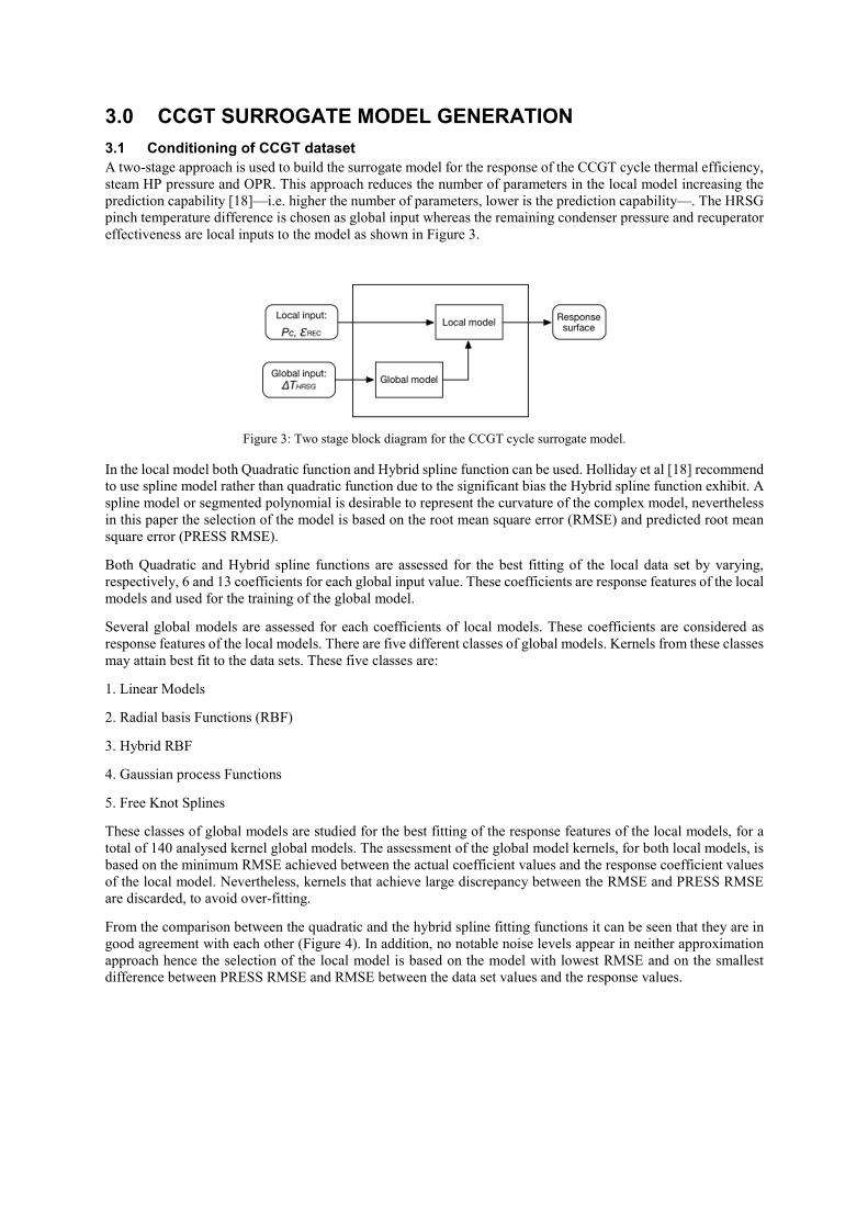
A two-stage approach is used to build the surrogate model for the response of the CCGT cycle thermal efficiency,steam HP pressure and OPR. This approach reduces the number of parameters in the local model increasing theprediction capability [18]—i.e. higher the number of parameters, lower is the prediction capability—. The HRSGpinch temperature difference is chosen as global input whereas the remaining condenser pressure and recuperatoreffectiveness are local inputs to the model as shown in Figure 3.

Figure 3: Two stage block diagram for the CCGT cycle surrogate model.

In the local model both Quadratic function and Hybrid spline function can be used. Holliday et al [18] recommendto use spline model rather than quadratic function due to the significant bias the Hybrid spline function exhibit. Aspline model or segmented polynomial is desirable to represent the curvature of the complex model, neverthelessin this paper the selection of the model is based on the root mean square error (RMSE) and predicted root meansquare error (PRESS RMSE).

Both Quadratic and Hybrid spline functions are assessed for the best fitting of the local data set by varying,respectively, 6 and 13 coefficients for each global input value. These coefficients are response features of the localmodels and used for the training of the global model.

Several global models are assessed for each coefficients of local models. These coefficients are considered asresponse features of the local models. There are five different classes of global models. Kernels from these classesmay attain best fit to the data sets. These five classes are:

1. Linear Models

2. Radial basis Functions (RBF)

3. Hybrid RBF

4. Gaussian process Functions

5. Free Knot Splines

These classes of global models are studied for the best fitting of the response features of the local models, for atotal of 140 analysed kernel global models. The assessment of the global model kernels, for both local models, isbased on the minimum RMSE achieved between the actual coefficient values and the response coefficient valuesof the local model. Nevertheless, kernels that achieve large discrepancy between the RMSE and PRESS RMSEare discarded, to avoid over-fitting.

From the comparison between the quadratic and the hybrid spline fitting functions it can be seen that they are ingood agreement with each other (Figure 4). In addition, no notable noise levels appear in neither approximationapproach hence the selection of the local model is based on the model with lowest RMSE and on the smallestdifference between PRESS RMSE and RMSE between the data set values and the response values.

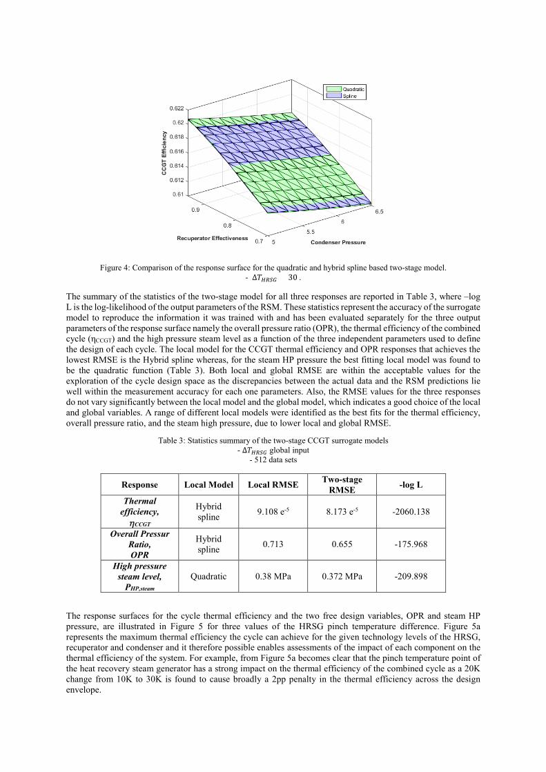
Figure 4: Comparison of the response surface for the quadratic and hybrid spline based two-stage model.- ∆����� = 30 .

The summary of the statistics of the two-stage model for all three responses are reported in Table 3, where –logL is the log-likelihood of the output parameters of the RSM. These statistics represent the accuracy of the surrogatemodel to reproduce the information it was trained with and has been evaluated separately for the three outputparameters of the response surface namely the overall pressure ratio (OPR), the thermal efficiency of the combinedcycle (ηCCGT) and the high pressure steam level as a function of the three independent parameters used to definethe design of each cycle. The local model for the CCGT thermal efficiency and OPR responses that achieves thelowest RMSE is the Hybrid spline whereas, for the steam HP pressure the best fitting local model was found tobe the quadratic function (Table 3). Both local and global RMSE are within the acceptable values for theexploration of the cycle design space as the discrepancies between the actual data and the RSM predictions liewell within the measurement accuracy for each one parameters. Also, the RMSE values for the three responsesdo not vary significantly between the local model and the global model, which indicates a good choice of the localand global variables. A range of different local models were identified as the best fits for the thermal efficiency,overall pressure ratio, and the steam high pressure, due to lower local and global RMSE.

Table 3: Statistics summary of the two-stage CCGT surrogate models- ∆����� global input

- 512 data sets

Response Local Model Local RMSETwo-stage

RMSE-log L

Thermalefficiency,ηCCGT

Hybridspline

9.108 e-5 8.173 e-5 -2060.138

Overall PressurRatio,OPR

Hybridspline

0.713 0.655 -175.968

High pressuresteam level,

PHP,steam

Quadratic 0.38 MPa 0.372 MPa -209.898

The response surfaces for the cycle thermal efficiency and the two free design variables, OPR and steam HPpressure, are illustrated in Figure 5 for three values of the HRSG pinch temperature difference. Figure 5arepresents the maximum thermal efficiency the cycle can achieve for the given technology levels of the HRSG,recuperator and condenser and it therefore possible enables assessments of the impact of each component on thethermal efficiency of the system. For example, from Figure 5a becomes clear that the pinch temperature point ofthe heat recovery steam generator has a strong impact on the thermal efficiency of the combined cycle as a 20Kchange from 10K to 30K is found to cause broadly a 2pp penalty in the thermal efficiency across the designenvelope.

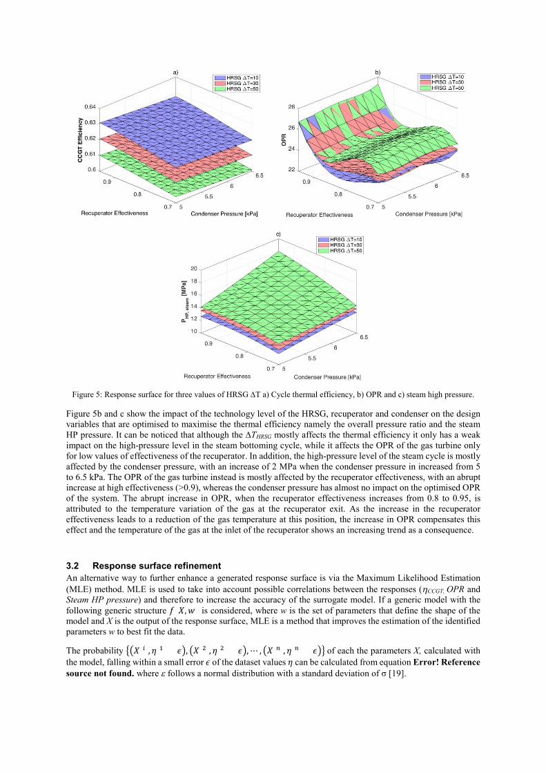
Figure 5: Response surface for three values of HRSG ∆T a) Cycle thermal efficiency, b) OPR and c) steam high pressure.

Figure 5b and c show the impact of the technology level of the HRSG, recuperator and condenser on the designvariables that are optimised to maximise the thermal efficiency namely the overall pressure ratio and the steamHP pressure. It can be noticed that although the ∆THRSG mostly affects the thermal efficiency it only has a weakimpact on the high-pressure level in the steam bottoming cycle, while it affects the OPR of the gas turbine onlyfor low values of effectiveness of the recuperator. In addition, the high-pressure level of the steam cycle is mostlyaffected by the condenser pressure, with an increase of 2 MPa when the condenser pressure in increased from 5to 6.5 kPa. The OPR of the gas turbine instead is mostly affected by the recuperator effectiveness, with an abruptincrease at high effectiveness (>0.9), whereas the condenser pressure has almost no impact on the optimised OPRof the system. The abrupt increase in OPR, when the recuperator effectiveness increases from 0.8 to 0.95, isattributed to the temperature variation of the gas at the recuperator exit. As the increase in the recuperatoreffectiveness leads to a reduction of the gas temperature at this position, the increase in OPR compensates thiseffect and the temperature of the gas at the inlet of the recuperator shows an increasing trend as a consequence.

3.2 Response surface refinement

An alternative way to further enhance a generated response surface is via the Maximum Likelihood Estimation(MLE) method. MLE is used to take into account possible correlations between the responses (ηCCGT, OPR andSteam HP pressure) and therefore to increase the accuracy of the surrogate model. If a generic model with thefollowing generic structure �(�,�) is considered, where w is the set of parameters that define the shape of themodel and X is the output of the response surface, MLE is a method that improves the estimation of the identifiedparameters w to best fit the data.

The probability ���(�), �(�) ± ��, ��(�), �(�) ± ��, ⋯ , ��(�), �(�) ± ���of each the parameters X, calculated with

the model, falling within a small error � of the dataset values � can be calculated from equation Error! Referencesource not found. where ε follows a normal distribution with a standard deviation of σ [19].

�����������, � =1

(2���)��

��exp �−1

2��(�) − �(�,�)

��

�

� ��

�

�

( 1 )

This probability ( Eq. Error! Reference source not found.) is defined as the likelihood of the parameters giventhe data [19]. In order to maximize the probability, the negative natural logarithm in equation 2 must be minimizedand the selection of w is updated.

min�

���(�) − �(�,�)

2���

�

���

− � ln � ( 2 )

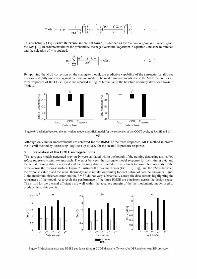
By applying the MLE correction on the surrogate model, the predictive capability of the surrogate for all threeresponses slightly improves against the baseline model. The model improvements due to the MLE method for allthree responses of the CCGT cycle are reported in Figure 6 relative to the baseline accuracy statistics shown inTable 3.

Figure 6: Variation between the uni-variate model and MLE model for the responses of the CCGT cycle, a) RMSE and b) –logL.

Although only minor improvements are achieved for the RMSE of the three responses, MLE method improvesthe overall method by decreasing –logL test up to 36% for the steam HP pressure response.

3.3 Validation of the CCGT surrogate model

The surrogate models generated previously were validated within the bounds of the training data using a so-calledsubset apparent validation approach. The error between the surrogate model response for the training data andthe actual training data is assessed and the training data is divided in five subsets to ensure homogeneity of theerrors across the response surface. Figure 7 illustrates the maximum error (��� = |� − �̂|) and the RMSE betweenthe response value �̂ and the actual thermodynamic simulation result � for each subset of data. As shown in Figure7, the maximum observed error and the RMSE do not vary substantially across the data subsets highlighting therobustness of the model. As a result the performance of the three RMSE are consistent across the design space.The errors for the thermal efficiency are well within the accuracy margin of the thermodynamic model used toproduce these data points.

Figure 7: Maximum error and RMSE per data subset a) CCGT thermal efficiency, b) OPR and c) steam HP pressure.

The generated surrogate models were also validated with a split sample validation, where the response surfaceswere used to produce 27 new predictions at certain positions within the design space where no data points existed

previously. The sampling of the values of the recuperator effectiveness, of the pinch temperature in the HRSGand of the pressure in the condenser of the steam cycle was generated using the Latin Hypercube Sampling method

[4] whereas the thermal efficiency of the system, high pressure in the steam cycle and OPR are a result of theoptimization process. The same 27 sample points were subsequently modelled on the TurboMatch - StemoMatchsimulation deck to generate a simulated cycle thermal efficiency, OPR and steam HP pressure level. The RMSE

and the maximum difference between the new samples values and the values obtained with the response surfacesare reported in Table 4.

Table 4: Statistics summary of split sample validation between simulated and approximated via the surrogate design points.- ∆����� global input

- 27 data sets

Response RMSE Maximum error

ηCCGT 7.14 e-5 1.358 e-4

OPR 0.67 1.42

Steam HP pressure 0.25 MPa 0.62 MPa

The discrepancy between the model prediction and the sample data from the split sample validation are within

acceptable values for the description of a design space of a complex system as a combined cycle. This addscredibility in the use of surrogate models for design space exploration of the complex gas-turbine systems.

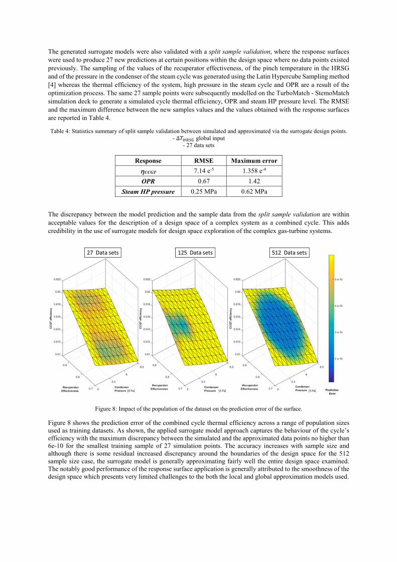
Figure 8: Impact of the population of the dataset on the prediction error of the surface.

Figure 8 shows the prediction error of the combined cycle thermal efficiency across a range of population sizesused as training datasets. As shown, the applied surrogate model approach captures the behaviour of the cycle’sefficiency with the maximum discrepancy between the simulated and the approximated data points no higher than6e-10 for the smallest training sample of 27 simulation points. The accuracy increases with sample size andalthough there is some residual increased discrepancy around the boundaries of the design space for the 512sample size case, the surrogate model is generally approximating fairly well the entire design space examined.The notably good performance of the response surface application is generally attributed to the smoothness of thedesign space which presents very limited challenges to the both the local and global approximation models used.

4.0 CONCLUSIONS

The methodology developed in the current paper shows the application of a response surface approach to capturethe performance of a complex power system across a defined design space. The method evaluates the selection ofthe best fitting local and global model, allowing a range of local models for each response (efficiency, overallpressure ratio, temperature pinch difference in the HRSG and HP steam pressure) to achieve the minimum RMSEfor each one of them. The analysis showed that the overall thermal efficiency and overall pressure ratio are bestdescribed by a hybrid spline local model while a quadratic local model showed the best fit to capture the variationsin the high pressure steam level. After the refinement of the response surface an improvement in the –logL test by35% for the pressure of the HP steam pressure was achieved. Finally, a subset apparent validation as well as asplit sample validation of the generated response surfaces showed that the employed models could successfullycapture the design space variations both within and beyond the initially defined design space with the total numberof training datasets slightly affecting the accuracy of the model.

This paper demonstrates the feasibility of using response surface approaches for describing the performance ofadvance cycles with multiple design variables. This helps in drastically reducing the modelling time and numberof thermodynamic simulations required as part of the preliminary evaluation of a design space and consequentlyproduce notable economies in computational time and resources during preliminary design phases. The responsesurface could be further used where several advance power cycles need to be evaluated as alternatives to a newsystem, coupled with cost, size and weight analyses tools, for example, to determine the impact of the technologylevel of the components on key design metrics of the power plant. A response surface would in that casesuccessfully replace the thermodynamic model of the cycle within the general application model. This can thenbe used for system optimization where the goal could be maximum thermal efficiency or minimum levelized costof the electricity.

REFERENCES

[1] G Koutsothanasis. Marine Gas Turbine Performance Model for Rim Driven Propeller & MoreElectric Architectures. PhD Thesis, Cranfield University, 2010.

[2] G Koutsothanasis, A I Kalfas and G Doulgeris. Marine Gas Turbine Performance Model forMore Electric Ships. In ASME Turbo Expo 2011: Power for Land, Sea, and Air, ASME, 2011.

[3] F Hempert. Rotorcraft engine cycle optimisation at mission level, PhD thesis, CranfieldUniversity, 2012.

[4] K Kritikos, E Giordano, A I Kalfas and N Tantot. Prediction of certification noise levelsgenerated by contra-rotating open rotor engines. In ASME Turbo Expo 2012: Power for Land,Sea, and Air, ASME, 2012.

[5] C Celis. Evaluation and Optimisation of Environmentally Friendly Aircraft Propulsion Systems.PhD thesis, Cranfield University, 2010.

[6] G Di Lorenzo. Advanced Low-Carbon Power Plants – the TERA Approach. PhD thesis,Cranfield University, 2010.

[7] S Mohaghegh. Surrogate Reservoir Model. In EGU General Assembly Conference, 12, p. 234,2010.

[8] F Bai, C H Lim, J Jia, K Santostefano, C Simmons, H Kasahara, W Wu, N Terada and S Jin.Directed Differentiation of Embryonic Stem Cells Into Cardiomyocytes by Bacterial Injection ofDefined Transcription Factors. Scientific Reports, 5, p. 15014, 2015.

[9] W L Macmillan. Development of a Module Type Computer Program for the Calculation of GasTurbine Off Design Performance. PhD thesis, Cranfield University, 1974.

[10] Y G Li, P Pilidis and M A Newby. An Adaptation Approach for Gas Turbine Design-PointPerformance Simulation. Journal of Engineering for Gas Turbines and Power, 128(4), pp. 789–795, 2006.

[11] M Mucino, Y G Li, J Ojile and M A Newby. Advanced performance modelling of a single anddouble pressure once through steam generator. In ASME Turbo Expo 2007: Power for Land, Sea,and Air, ASME, 2007.

[12] E M Goodger and S O T Ogaji, Fuels and Combustion in Heat Engines, Cranfield Design + Print,2011.

[13] J B Young and R C Wilcock. Modeling the Air-Cooled Gas Turbine: Part 2—Coolant Flows andLosses. J. Turbomach, 124(2), pp. 214–8, 2002.

[14] J H Horlock, D T Watson and T V Jones. Limitations on Gas Turbine Performance Imposed byLarge Turbine Cooling Flows. J. Eng. Gas Turbines Power, 123(3), p. 487, 2001.

[15] R Kehlhofer, F Hannemann, B Rukes and F Stirnimann. Combined-Cycle Gas & Steam TurbinePower Plants. PennWell Books, 2009.

[16] V Ganapathy. Steam Generators and Waste Heat Boilers. CRC Press, 2014.[17] K Deb. Multi-Objective Optimization Using Evolutionary Algorithms. John Wiley & Sons, 2001.[18] T Holliday, A J Lawrance and T P Davis. Engine-Mapping Experiments: A Two-Stage

Regression Approach. Technometrics, 2012.[19] A Forrester, D A Sobester and D A Keane. Engineering Design via Surrogate Modelling. John

Wiley & Sons, 2008.