Embed Size (px)
Citation preview

HEWLETT-PACKARD
HP-15C ADVANCED FUNCTIONS
HANDBOOK

Legal Notice
This manual and any examples contained herein are provided “as is” and are subject to change
without notice. Hewlett-Packard Company makes no warranty of any kind with regard to this manual,
including, but not limited to, the implied warranties of merchantability non-infringement and fitness for
a particular purpose. In this regard, HP shall not be liable for technical or editorial errors or omissions
contained in the manual.
Hewlett-Packard Company shall not be liable for any errors or incidental or consequential damages in
connection with the furnishing, performance, or use of this manual or the examples contained herein.
Copyright © 1982, 2012 Hewlett-Packard Development Company, LP.
Reproduction, adaptation, or translation of this manual is prohibited without prior written permission of
Hewlett-Packard Company, except as allowed under the copyright laws.
Hewlett-Packard Company
Palo Alto, CA
94304
USA
HEWLETT PACKARD
HP-15C
Advanced Functions Handbook
August 1982
00015-90011
Printed in U.S.A.
© Hewlett-Packard Company 1982
4
Contents
Contents ...............................................................................................................4
Introduction .........................................................................................................7
Section 1: Using _ Effectively ..................................................................9 Finding Roots .........................................................................................................................9
How _ Samples ............................................................................................................9
Handling Troublesome Situations ........................................................................................11
Easy Versus Hard Equations .............................................................................................11
Inaccurate Equations .........................................................................................................12
Equations With Several Roots ..........................................................................................12
Using _ With Polynomials .........................................................................................12
Solving a System of Equations .............................................................................................16
Finding Local Extremes of a Function .................................................................................18
Using the Derivative .........................................................................................................18
Using an Approximate Slope ............................................................................................20
Using Repeated Estimation ...............................................................................................22
Applications ..........................................................................................................................24
Annuities and Compound Amounts ..................................................................................24
Discounted Cash Flow Analysis .......................................................................................34
Section 2: Working with f .......................................................................... 40 Numerical Integration Using f ........................................................................................40
Accuracy of the Function to be Integrated ...........................................................................41
Functions Related to Physical Situations ..........................................................................42
Round-Off Error in Internal Calculations .........................................................................42
Shortening Calculation Time ................................................................................................43
Subdividing the Interval of Integration .............................................................................43
Transformation of Variables .............................................................................................47
Evaluating Difficult Integrals ...............................................................................................48
Application ...........................................................................................................................51
Section 3: Calculating in Complex Mode ...................................................... 56
Using Complex Mode ...........................................................................................................56
Trigonometric Modes ...........................................................................................................58
Definitions of Math Functions ..............................................................................................59
Arithmetic Operations .......................................................................................................59
Single Valued Functions ...................................................................................................59
Multivalued Functions ......................................................................................................59
Using _ and f in Complex Mode ..........................................................................63
Accuracy in Complex Mode .................................................................................................63
Contents 5
Applications ......................................................................................................................... 65
Storing and Recalling Complex Numbers Using a Matrix .............................................. 65
Calculating the nth Roots of a Complex Number ............................................................ 67
Solving an Equation for Its Complex Roots .................................................................... 69
Contour Integrals .............................................................................................................. 73
Complex Potentials .......................................................................................................... 76
Section 4: Using Matrix Operations ................................................................ 82
Understanding the LU Decomposition ................................................................................ 82
ILL-Conditioned Matrices and the Condition Number ....................................................... 84
The Accuracy of Numerical Solutions to Linear Systems .................................................. 87
Making Difficult Equations Easier ...................................................................................... 88
Scaling .............................................................................................................................. 88
Preconditioning ................................................................................................................ 91
Least-Squares Calculations.................................................................................................. 93
Normal Equations ............................................................................................................. 93
Orthogonal Factorization.................................................................................................. 95
Singular and Nearly Singular Matrices ............................................................................... 98
Applications ....................................................................................................................... 100
Constructing an Identity Matrix ..................................................................................... 100
One-Step Residual Correction ........................................................................................ 101
Solving a System of Nonlinear Equations ..................................................................... 102
Solving a Large System of Complex Equations............................................................. 108
Least-Squares Using Normal Equations ........................................................................ 111
Least-Squares Using Successive Rows .......................................................................... 118
Eigenvalues of a Symmetric Real Matrix ...................................................................... 125
Eigenvectors of a Symmetric Real Matrix ..................................................................... 130
Optimization ................................................................................................................... 135
Appendix: Accuracy of Numerical Calculations ......................................... 145
Misconceptions About Errors ............................................................................................ 145
A Hierarchy of Errors ........................................................................................................ 150
Level 0: No Error ............................................................................................................... 150
Level ∞: Overflow/Underflow ......................................................................................... 150
Level 1: Correctly Rounded, or Nearly So ........................................................................ 150
Level 1C: Complex Level 1............................................................................................... 153
Level 2: Correctly Rounded for Possibly Perturbed Input ................................................ 154
Trigonometric Functions of Real Radian Angles ........................................................... 154
Backward Error Analysis ............................................................................................... 157
Backward Error Analysis Versus Singularities .............................................................. 161
Summary to Here ........................................................................................................... 162
Backward Error Analysis of Matrix Inversion ............................................................... 168
Is Backward Error Analysis a Good Idea? ..................................................................... 171
Index ................................................................................................................. 178

6

7
Introduction
The HP-15C provides several advanced capabilities never before combined so conveniently
in a handheld calculator:
Finding the roots of equations.
Evaluating definite integrals.
Calculating with complex numbers.
Calculating with matrices.
The HP-15C Owner's Handbook gives the basic information about performing these
advanced operations. It also includes numerous examples that show how to use these
features. The owner's handbook is your primary reference for information about the advanced
functions.
This HP-15C Advanced Functions Handbook continues where the owner's handbook leaves
off. In this handbook you will find information about how the HP-15C performs the
advanced computations and information that explains how to interpret the results that you
get.
This handbook also contains numerous programs, or applications. These programs serve two
purposes. First, they suggest ways of using the advanced functions, so that you might use
these capabilities more effectively in your own applications. Second, the programs cover a
wide range of applications—they may be useful to you in the form presented in this
handbook.
Note: The discussions of most topics in this handbook presume that you
already understand the basic information about using the advanced functions
and that you are generally familiar with the subject matter being discussed.

8
9
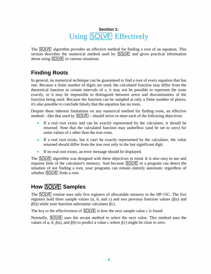
Section 1: Using _ Effectively
The _ algorithm provides an effective method for finding a root of an equation. This
section describes the numerical method used by _ and gives practical information
about using _ in various situations.
Finding Roots
In general, no numerical technique can be guaranteed to find a root of every equation that has
one. Because a finite number of digits are used, the calculated function may differ from the
theoretical function in certain intervals of x, it may not be possible to represent the roots
exactly, or it may be impossible to distinguish between zeros and discontinuities of the
function being used. Because the function can be sampled at only a finite number of places,
it's also possible to conclude falsely that the equation has no roots.
Despite these inherent limitations on any numerical method for finding roots, an effective
method—like that used by _—should strive to meet each of the following objectives:
If a real root exists and can be exactly represented by the calculator, it should be
returned. Note that the calculated function may underflow (and be set to zero) for
some values of x other than the true roots.
If a real root exists, but it can't be exactly represented by the calculator, the value
returned should differ from the true root only in the last significant digit.
If no real root exists, an error message should be displayed.
The _ algorithm was designed with these objectives in mind. It is also easy to use and
requires little of the calculator's memory. And because _ in a program can detect the
situation of not finding a root, your programs can remain entirely automatic regardless of
whether _ finds a root.
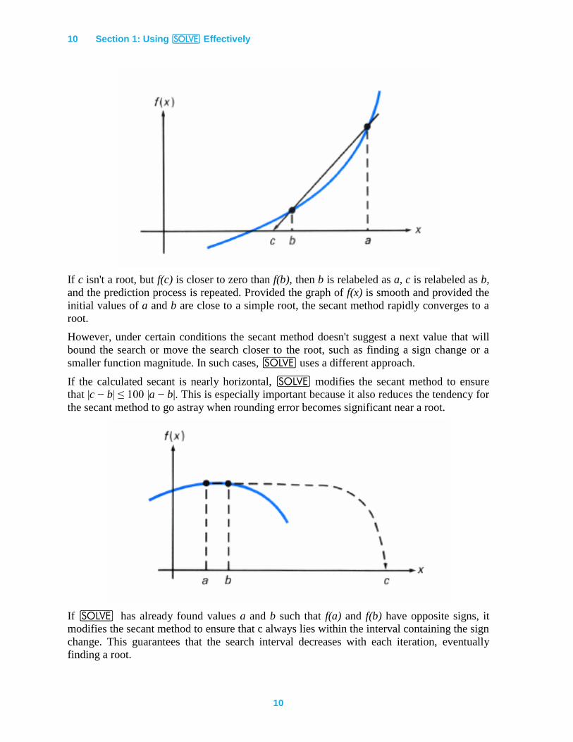
How _ Samples
The _ routine uses only five registers of allocatable memory in the HP-15C. The five
registers hold three sample values (a, b, and c) and two previous function values (f(a) and
f(b)) while your function subroutine calculates f(c).
The key to the effectiveness of _ is how the next sample value c is found.
Normally, _ uses the secant method to select the next value. This method uses the
values of a, b, f(a), and f(b) to predict a value c where f(c) might be close to zero.
10 Section 1: Using _ Effectively
10
If c isn't a root, but f(c) is closer to zero than f(b), then b is relabeled as a, c is relabeled as b,
and the prediction process is repeated. Provided the graph of f(x) is smooth and provided the
initial values of a and b are close to a simple root, the secant method rapidly converges to a
root.
However, under certain conditions the secant method doesn't suggest a next value that will
bound the search or move the search closer to the root, such as finding a sign change or a
smaller function magnitude. In such cases, _ uses a different approach.
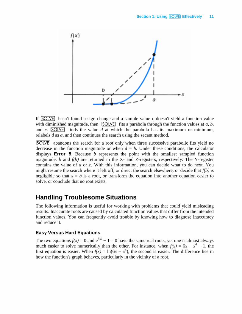
If the calculated secant is nearly horizontal, _ modifies the secant method to ensure
that |c − b| ≤ 100 |a − b|. This is especially important because it also reduces the tendency for
the secant method to go astray when rounding error becomes significant near a root.
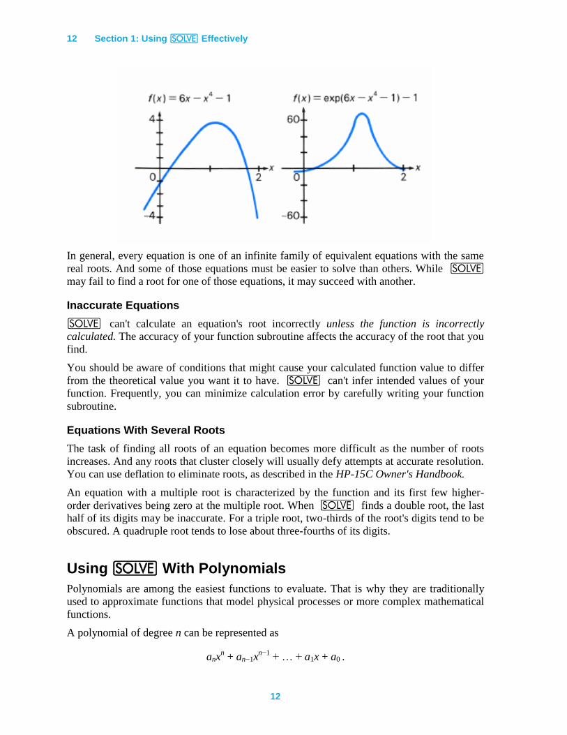
If _ has already found values a and b such that f(a) and f(b) have opposite signs, it
modifies the secant method to ensure that c always lies within the interval containing the sign
change. This guarantees that the search interval decreases with each iteration, eventually
finding a root.
Section 1: Using _ Effectively 11
If _ hasn't found a sign change and a sample value c doesn't yield a function value
with diminished magnitude, then _ fits a parabola through the function values at a, b,
and c. _ finds the value d at which the parabola has its maximum or minimum,
relabels d as a, and then continues the search using the secant method.
_ abandons the search for a root only when three successive parabolic fits yield no
decrease in the function magnitude or when d = b. Under these conditions, the calculator
displays Error 8. Because b represents the point with the smallest sampled function
magnitude, b and f(b) are returned in the X- and Z-registers, respectively. The Y-register
contains the value of a or c. With this information, you can decide what to do next. You
might resume the search where it left off, or direct the search elsewhere, or decide that f(b) is
negligible so that x = b is a root, or transform the equation into another equation easier to
solve, or conclude that no root exists.
Handling Troublesome Situations
The following information is useful for working with problems that could yield misleading
results. Inaccurate roots are caused by calculated function values that differ from the intended
function values. You can frequently avoid trouble by knowing how to diagnose inaccuracy
and reduce it.
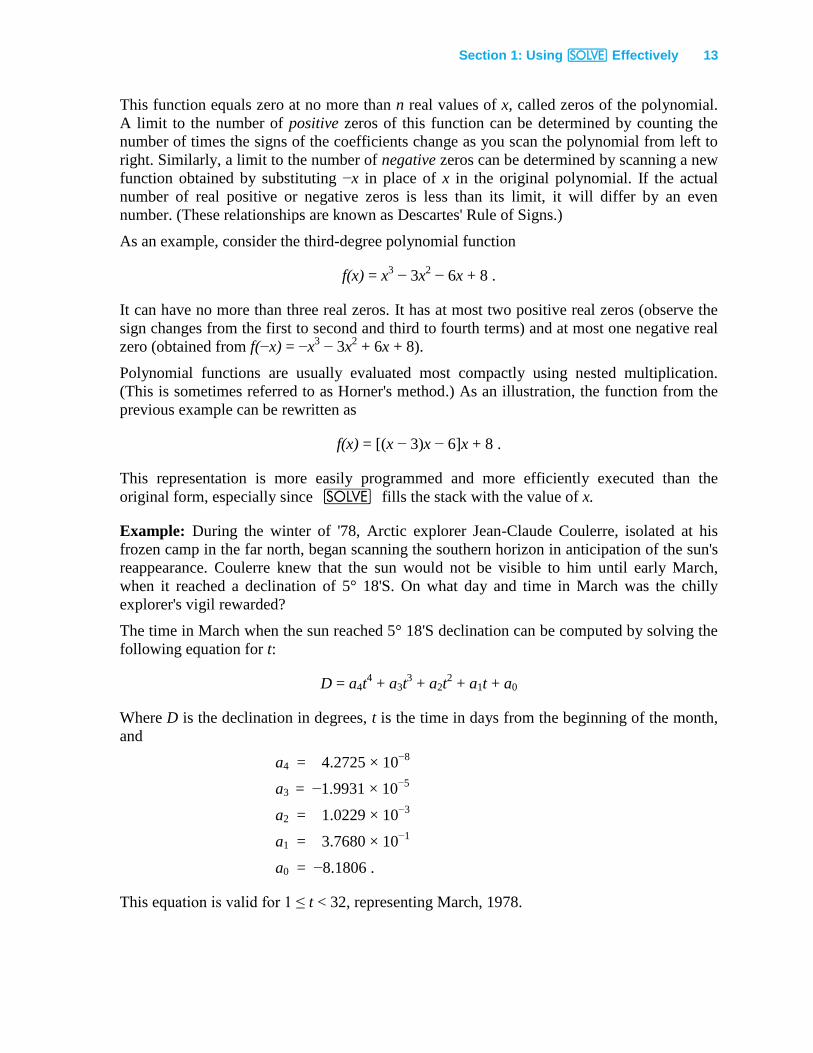
Easy Versus Hard Equations
The two equations f(x) = 0 and ef(x)
− 1 = 0 have the same real roots, yet one is almost always
much easier to solve numerically than the other. For instance, when f(x) = 6x − x4 − 1, the
first equation is easier. When f(x) = ln(6x − x4), the second is easier. The difference lies in
how the function's graph behaves, particularly in the vicinity of a root.
12 Section 1: Using _ Effectively
12
In general, every equation is one of an infinite family of equivalent equations with the same
real roots. And some of those equations must be easier to solve than others. While _
may fail to find a root for one of those equations, it may succeed with another.
Inaccurate Equations
_ can't calculate an equation's root incorrectly unless the function is incorrectly
calculated. The accuracy of your function subroutine affects the accuracy of the root that you
find.
You should be aware of conditions that might cause your calculated function value to differ
from the theoretical value you want it to have. _ can't infer intended values of your
function. Frequently, you can minimize calculation error by carefully writing your function
subroutine.
Equations With Several Roots
The task of finding all roots of an equation becomes more difficult as the number of roots
increases. And any roots that cluster closely will usually defy attempts at accurate resolution.
You can use deflation to eliminate roots, as described in the HP-15C Owner's Handbook.
An equation with a multiple root is characterized by the function and its first few higher-
order derivatives being zero at the multiple root. When _ finds a double root, the last
half of its digits may be inaccurate. For a triple root, two-thirds of the root's digits tend to be
obscured. A quadruple root tends to lose about three-fourths of its digits.
Using _ With Polynomials
Polynomials are among the easiest functions to evaluate. That is why they are traditionally
used to approximate functions that model physical processes or more complex mathematical
functions.
A polynomial of degree n can be represented as
anxn + an−1x
n−1 + … + a1x + a0 .
Section 1: Using _ Effectively 13
This function equals zero at no more than n real values of x, called zeros of the polynomial.
A limit to the number of positive zeros of this function can be determined by counting the
number of times the signs of the coefficients change as you scan the polynomial from left to
right. Similarly, a limit to the number of negative zeros can be determined by scanning a new
function obtained by substituting −x in place of x in the original polynomial. If the actual
number of real positive or negative zeros is less than its limit, it will differ by an even
number. (These relationships are known as Descartes' Rule of Signs.)
As an example, consider the third-degree polynomial function
f(x) = x3 − 3x
2 − 6x + 8 .
It can have no more than three real zeros. It has at most two positive real zeros (observe the
sign changes from the first to second and third to fourth terms) and at most one negative real
zero (obtained from f(−x) = −x3 − 3x
2 + 6x + 8).
Polynomial functions are usually evaluated most compactly using nested multiplication.
(This is sometimes referred to as Horner's method.) As an illustration, the function from the
previous example can be rewritten as
f(x) = [(x − 3)x − 6]x + 8 .
This representation is more easily programmed and more efficiently executed than the
original form, especially since _ fills the stack with the value of x.
Example: During the winter of '78, Arctic explorer Jean-Claude Coulerre, isolated at his
frozen camp in the far north, began scanning the southern horizon in anticipation of the sun's
reappearance. Coulerre knew that the sun would not be visible to him until early March,
when it reached a declination of 5° 18'S. On what day and time in March was the chilly
explorer's vigil rewarded?
The time in March when the sun reached 5° 18'S declination can be computed by solving the
following equation for t:
D = a4t4 + a3t
3 + a2t
2 + a1t + a0
Where D is the declination in degrees, t is the time in days from the beginning of the month,
and
a4 = 4.2725 × 10⁻⁸
a3 = −1.9931 × 10⁻⁵
a2 = 1.0229 × 10⁻³
a1 = 3.7680 × 10⁻¹
a0 = −8.1806 .
This equation is valid for 1 ≤ t < 32, representing March, 1978.
14 Section 1: Using _ Effectively
14
First convert 5° 18'S to decimal degrees (press 5.18”|À), obtaining −5.3000
(using •4 display mode). (Southern latitudes are expressed as negative numbers for
calculation purposes.)
The solution to Coulerre's problems is the value of t satisfying
−5.3000 = a4t4 + a3t
3 + a2t
2 + a1t + a0.
Expressed in the form required by _ the equation is
0 = a4t4 + a3t
3 + a2t
2 + a1t − 2.8806
where the last, constant term now incorporates the value of the declination.
Using Horner's method, the function to be set equal to zero is
f(t) = (((a4t + a3)t + a2)t + a1)t − 2.8806 .
To shorten the subroutine, store and recall the constants using the registers corresponding to
the exponent of t.
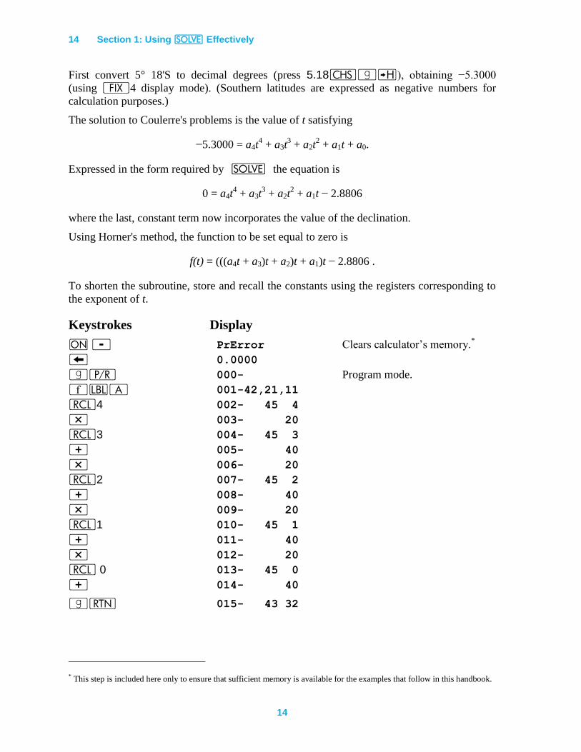
Keystrokes Display
= - PrError Clears calculator’s memory.*
− 0.0000
|¥ 000- Program mode.
´bA 001-42,21,11
l4 002- 45 4
* 003- 20
l3 004- 45 3
+ 005- 40
* 006- 20
l2 007- 45 2
+ 008- 40
* 009- 20
l1 010- 45 1
+ 011- 40
* 012- 20
l 0 013- 45 0
+ 014- 40
|n 015- 43 32
* This step is included here only to ensure that sufficient memory is available for the examples that follow in this handbook.
Section 1: Using _ Effectively 15
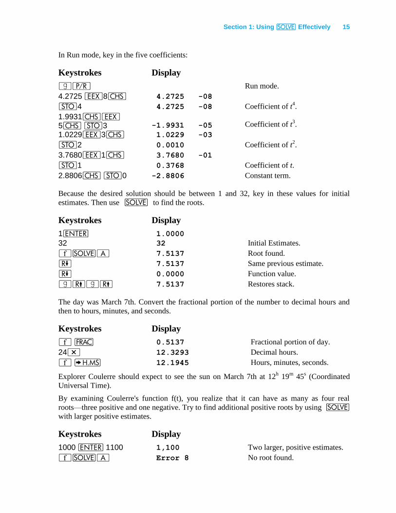
In Run mode, key in the five coefficients:
Keystrokes Display
|¥ Run mode.
4.2725 “8” 4.2725 -08
O4 4.2725 -08 Coefficient of t4.
1.9931”“ 5” O3 -1.9931 -05 Coefficient of t
3.
1.0229“3” 1.0229 -03
O2 0.0010 Coefficient of t2.
3.7680“1” 3.7680 -01
O1 0.3768 Coefficient of t.
2.8806” O0 -2.8806 Constant term.
Because the desired solution should be between 1 and 32, key in these values for initial
estimates. Then use _ to find the roots.
Keystrokes Display
1v 1.0000
32 32 Initial Estimates.
´_A 7.5137 Root found.
) 7.5137 Same previous estimate.
) 0.0000 Function value.
|(|( 7.5137 Restores stack.
The day was March 7th. Convert the fractional portion of the number to decimal hours and
then to hours, minutes, and seconds.
Keystrokes Display
´ q 0.5137 Fractional portion of day.
24* 12.3293 Decimal hours.
´ h 12.1945 Hours, minutes, seconds.
Explorer Coulerre should expect to see the sun on March 7th at 12h 19
m 45
s (Coordinated
Universal Time).
By examining Coulerre's function f(t), you realize that it can have as many as four real
roots—three positive and one negative. Try to find additional positive roots by using _
with larger positive estimates.
Keystrokes Display
1000 v 1100 1,100 Two larger, positive estimates.
´_A Error 8 No root found.
16 Section 1: Using _ Effectively
16
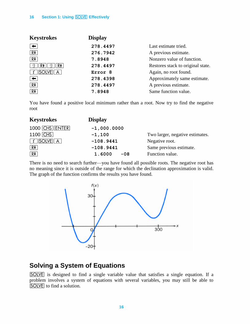
Keystrokes Display
− 278.4497 Last estimate tried.
) 276.7942 A previous estimate.
) 7.8948 Nonzero value of function.
|(|( 278.4497 Restores stack to original state.
´_A Error 8 Again, no root found.
− 278.4398 Approximately same estimate.
) 278.4497 A previous estimate.
) 7.8948 Same function value.
You have found a positive local minimum rather than a root. Now try to find the negative
root
Keystrokes Display
1000 ”v -1,000.0000
1100 ” -1,100 Two larger, negative estimates.
´_A -108.9441 Negative root.
) -108.9441 Same previous estimate.
) 1.6000 -08 Function value.
There is no need to search further—you have found all possible roots. The negative root has
no meaning since it is outside of the range for which the declination approximation is valid.
The graph of the function confirms the results you have found.
Solving a System of Equations
_ is designed to find a single variable value that satisfies a single equation. If a
problem involves a system of equations with several variables, you may still be able to
_ to find a solution.
Section 1: Using _ Effectively 17
For some systems of equations, expressed as
f1(x1, …, xn) = 0
⋮
fn(x1, …, xn) = 0
it is possible through algebraic manipulation to eliminate all but one variable. That is, you
can use the equations to derive expressions for all but one variable in terms of the remaining
variable. By using these expressions, you can reduce the problem to using _ to find
the root of a single equation. The values of the other variables at the solution can then be
calculated using the derived expressions.
This is often useful for solving a complex equation for a complex root. For such a problem,
the complex equation can be expressed as two real-valued equations—one for the real
component and one for the imaginary component—with two real variables—representing the
real and imaginary parts of the complex root.
For example, the complex equation z + 9 + 8e−z
= 0 has no real roots z, but it has infinitely
many complex roots z = x + iy. This equation can be expressed as two real equations
x + 9 + 8e−x
cos y = 0
y − 8e−x
sin y = 0.
The following manipulations can be used to eliminate y from the equations. Because the sign
of y doesn't matter in the equations, assume y > 0, so that any solution (x,y) gives another
solution (x,−y). Rewrite the second equation as
x = ln(8(sin y)/y),
which requires that sin y > 0, so that 2nπ < y < (2n + 1)π for integer n = 0, 1, ....
From the first equation
y = cos−1
(−ex(x + 9)/8) + 2nπ
= (2n + 1)π − cos−1
(ex(x + 9)/8)
for n = 0, 1, … substitute this expression into the second equation,
0))9((64
)8/)9((cos)12(ln
2
1
xe
xenx
x
x.
You can then use _ to find the root x of this equation (for any given value of n, the
number of the root). Knowing x, you can calculate the corresponding value of y.
18 Section 1: Using _ Effectively
18
A final consideration for this example is to choose the initial estimates that would be
appropriate. Because the argument of the inverse cosine must be between −1 and 1, x must be
more negative than about −0.1059 (found by trial and error or by using _). The initial
guesses might be near but more negative than this value, −0.11 and −0.2 for example.
(The complex equation used in this example is solved using an iterative procedure in the
example on page 69. Another method for solving a system of nonlinear equations is
described on page 102.)
Finding Local Extremes of a Function
Using the Derivative
The traditional way to find local maximums and minimums of a function's graph uses the
derivative of the function. The derivative is a function that describes the slope of the graph.
Values of x at which the derivative is zero represent potential local extremes of the function.
(Although less common for well-behaved functions, values of x where the derivative is
infinite or undefined are also possible extremes.) If you can express the derivative of a
function in closed form, you can use _ to find where the derivative is zero—showing
where the function may be maximum or minimum.
Example: For the design of a vertical broadcasting tower, radio engineer Ann Tenor wants to
find the angle from the tower at which the relative field intensity is most negative. The
relative intensity created by the tower is given by
sin)]2cos(1[
)2cos()cos2cos(
h
hhE
where E is the relative field intensity, h is the antenna height in wavelengths, and θ is the
angle from vertical in radians. The height is 0.6 wavelengths for her design.
The desired angle is one at which the derivative of the intensity with respect to θ is zero.
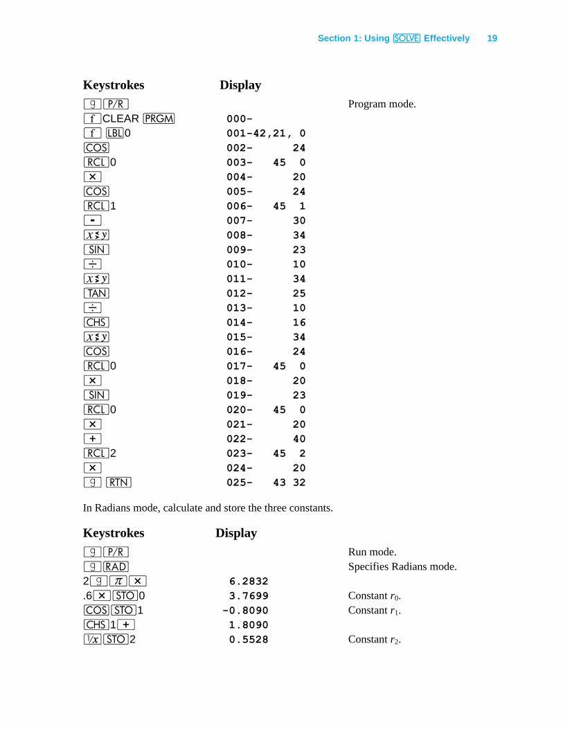
To save program memory space and execution time, store the following constants in registers
and recall them as needed:
r0 = 2πh and is stored in register R0,
r1 = cos(2πh) and is stored in register R1,
r2 = 1/[1 − cos(2πh)] and is stored in register R2.
The derivative of the intensity E with respect to the angle θ is given by
tansin
)coscos()cossin( 10
002
rrrrr
d
dE
.
Key in a subroutine to calculate the derivative.
Section 1: Using _ Effectively 19
Keystrokes Display
|¥ Program mode.
´CLEAR M 000-
´ b0 001-42,21, 0
\ 002- 24
l0 003- 45 0
* 004- 20
\ 005- 24
l1 006- 45 1
- 007- 30
® 008- 34
[ 009- 23
÷ 010- 10
® 011- 34
] 012- 25
÷ 013- 10
” 014- 16
® 015- 34
\ 016- 24
l0 017- 45 0
* 018- 20
[ 019- 23
l0 020- 45 0
* 021- 20
+ 022- 40
l2 023- 45 2
* 024- 20
| n 025- 43 32
In Radians mode, calculate and store the three constants.
Keystrokes Display
|¥ Run mode.
|R Specifies Radians mode.
2|$* 6.2832
.6*O0 3.7699 Constant r0.
\O1 -0.8090 Constant r1.
”1+ 1.8090
⁄O2 0.5528 Constant r2.
20 Section 1: Using _ Effectively
20
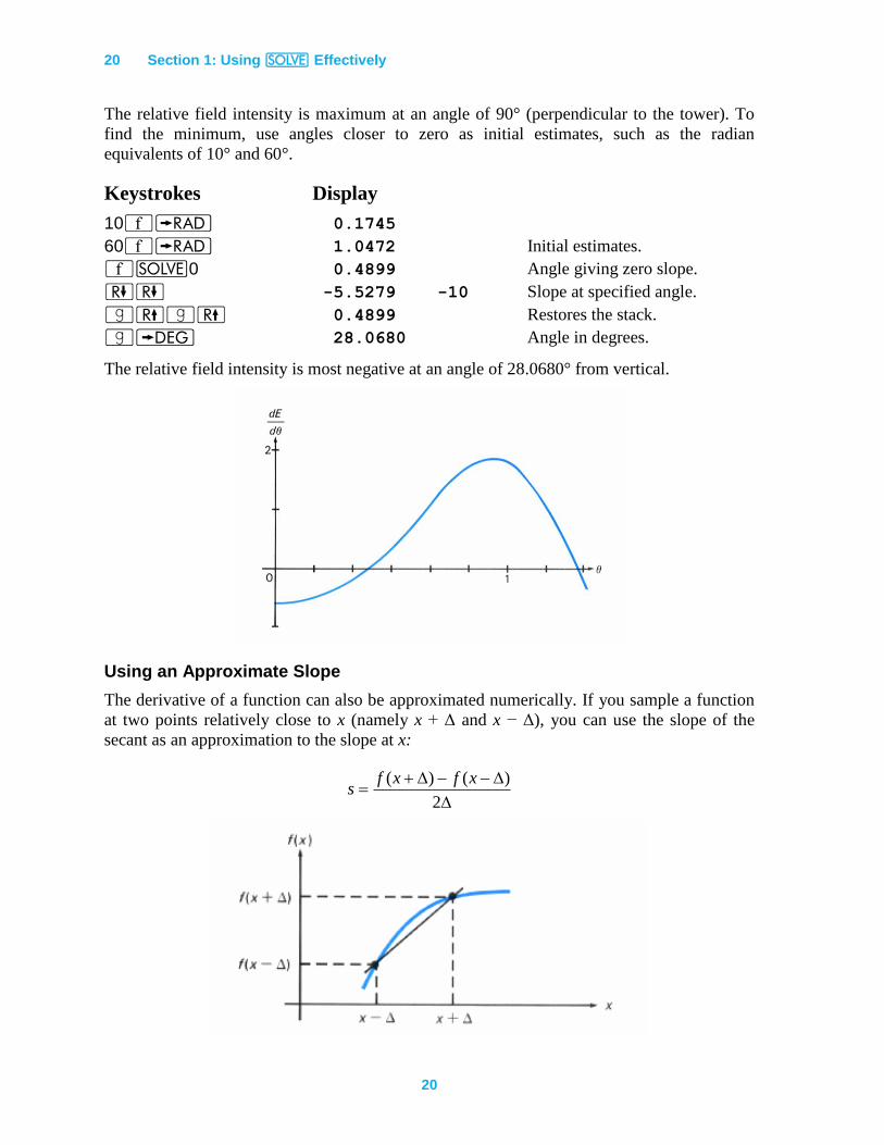
The relative field intensity is maximum at an angle of 90° (perpendicular to the tower). To
find the minimum, use angles closer to zero as initial estimates, such as the radian
equivalents of 10° and 60°.
Keystrokes Display
10´r 0.1745
60´r 1.0472 Initial estimates.
´_0 0.4899 Angle giving zero slope.
)) -5.5279 -10 Slope at specified angle.
|(|( 0.4899 Restores the stack.
|d 28.0680 Angle in degrees.
The relative field intensity is most negative at an angle of 28.0680° from vertical.
Using an Approximate Slope
The derivative of a function can also be approximated numerically. If you sample a function
at two points relatively close to x (namely x + Δ and x − Δ), you can use the slope of the
secant as an approximation to the slope at x:
2
)()( xfxfs
Section 1: Using _ Effectively 21
The accuracy of this approximation depends upon the increment Δ and the nature of the
function. Smaller values of Δ give better approximations to the derivative, but excessively
small values can cause round-off inaccuracy. A value of x at which the slope is zero is
potentially a local extreme of the function.
Example: Solve the previous example without using the equation for the derivative dE/dθ.
Find the angle at which the derivative (determined numerically) of the intensity E is zero.
In Program mode, key in two subroutines: one to estimate the derivative of the intensity and
one to evaluate the intensity function E. In the following subroutine, the slope is calculated
between θ + 0.001 and θ − 0.001 radians (a range equivalent to approximately 0.1°).
Keystrokes Display
|¥ 000- Program mode.
´bA 001-42,21,11
“ 002- 26
” 003- 16
3 004- 3 Evaluates E at θ + 0.001.
+ 005- 40
v 006- 36
GB 007- 32 12
® 008- 34
“ 009- 26
” 010- 16
3 011- 3 Evaluates E at θ − 0.001.
- 012- 30
v 013- 36
GB 014- 32 12
- 015- 30
2 016- 2
“ 017- 26
” 018- 16
3 019- 3
÷ 020- 10
|n 021- 43 32
´bB 022-42,21,12 Subroutine for E(θ).
\ 023- 24
l0 024- 45 0
* 025- 20
\ 026- 24
l1 027- 45 1
- 028- 30
22 Section 1: Using _ Effectively
22
Keystrokes Display
® 029- 34
[ 030- 23
÷ 031- 10
l2 032- 45 2
* 033- 20
|n 034- 43 32
In the previous example, the calculator was set to Radians mode and the three constants were
stored in registers R0, R1, and R2. Key in the same initial estimates as before and execute
_.
Keystrokes Display
|¥ Run mode.
10´r 0.1745
60´r 1.0472 Initial estimates.
´_A 0.4899 Angle given zero slope.
)) 0.0000 Slope at specified angle.
|(|( 0.4899 Restores stack.
vv´B -0.2043 Uses function subroutine to
calculate minimum intensity.
® 0.4899 Recalls θ value.
|d 28.0679 Angle in degrees.
This numerical approximation of the derivative indicates a minimum field intensity of
−0.2043 at an angle of 28.0679°. (This angle differs from the previous solution by 0.0001°.)
Using Repeated Estimation
A third technique is useful when it isn't practical to calculate the derivative. It is a slower
method because it requires the repeated use of the _ key. On the other hand, you
don't have to find a good value for Δ of the previous method. To find a local extreme of the
function f(x), define a new function
g(x) = f(x) − e
where e is a number slightly beyond the estimated extreme value of f(x). If e is properly
chosen, g(x) will approach zero near the extreme of f(x) but will not equal zero. Use _
to analyze g(x) near the extreme. The desired result is Error 8.
If Error 8 is displayed, the number in the X-register is an x value near the extreme.
The number in the Z-register tells roughly how far e is from the extreme value of f(x).
Revise e to bring it closer (but not equal) to the extreme value. Then use _ to
examine the revised g(x) near the x value previously found. Repeat this procedure
until successive x values do not differ significantly.
Section 1: Using _ Effectively 23
If a root of g(x) is found, either the number e is not beyond the extreme value of f(x)
or else _ has found a different region where f(x) equals e. Revise e so that it is
close to—but beyond—the extreme value of f(x) and try _ again. It may also
be possible to modify g(x) in order to eliminate the distant root.
Example: Solve the previous example without calculating the derivative of the relative field
intensity E.
The subroutine to calculate E and the required constants have been entered in the previous
example.
In Program mode, key in a subroutine that subtracts an estimated extreme number from the
field intensity E. The extreme number should be stored in a register so that it can be manually
changed as needed.
Keystrokes Display
|¥ 000- Program mode.
´b1 001-42,21, 1 Begins with label.
GB 002- 32 12 Calculates E.
l9 003- 45 9
- 004- 30 Subtracts extreme estimate.
|n 005- 43 32
In Run mode, estimate the minimum intensity value by manually sampling the function.
Keystrokes Display
|¥ Run mode.
10´r 0.1745
v´B -0.1029
30´r 0.5236 Samples the function at
v´B -0.2028 10°, 30°, 50°, …
50´r 0.8727
v´B 0.0405
24 Section 1: Using _ Effectively
24
Based on these samples, try using an extreme estimate of −0.25 and initial _
estimates (in radians ) near 10° and 30°.
Keystrokes Display
.25”O9 -0.2500 Stores extreme estimate.
.2v 0.2000
.6 0.6 Initial estimates.
´_1 Error 8 No root found.
−O4 0.4849 Stores θ estimate.
)O5 0.4698 Stores previous θ estimate.
) 0.0457 Distance from extreme.
.9* 0.0411 Revises extreme estimate
by 90 percent of the distance. O+9 0.0411
l4 0.4849 Recalls θ estimate.
vv´B -0.2043 Calculates intensity E.
− 0.0000 Recalls other θ estimate,
keeping first estimate in Y-
register. l5 0.4698
´_1 Error 8 No root found.
− 0.4898 θ estimate.
® 0.4893 Previous θ estimate.
® 0.4898 Recalls θ estimate.
vv´B -0.2043 Calculates intensity E.
® 0.4898 Recalls θ value.
|d 28.0660 Angle in degrees.
|D 28.0660 Restores Degrees mode.
The second interaction produces two θ estimates that differ in the fourth decimal place. The
field intensities E for the two iterations are equal to four decimal places. Stopping at this
point, a minimum field intensity of −0.2043 is indicated at an angle of 28.0660°. (This angle
differs from the previous solutions by about 0.002°.)
Applications
The following applications illustrate how you can use _ to simplify a calculation that
would normally be difficult—finding an interest rate that can't be calculated directly. Other
applications that use the _ function are given in Sections 3 and 4.
Annuities and Compound Amounts
This program solves a variety of financial problems involving money, time, and interest. For
these problems, you normally know the values of three or four of the following variables and
need to find the value of another:
Section 1: Using _ Effectively 25
n The number of compounding periods. (For example, a 30 year loan with monthly
payments has n = 12 x 30 = 360.)
i The interest rate per compounding period expressed as a percent. (To calculate i,
divide the annual percentage rate by the number of compounding periods in a year.
That is, 12% annual interest compounded monthly equals 1% periodic interest.)
PV The present value of a series of future cash flows or the initial cash flow.
PMT The periodic payment amount.
FV The future value. That is, the final cash flow (balloon payment or remaining balance)
or the compounded value of a series of prior cash flows.
Possible Problems Involving Annuities and Compound Amounts
Allowable Combinations of
Variables
Typical Applications
Initial Procedure For Payments at End of Period
For Payments at Beginning of Period
n, i, PV, PMT (Enter any three and calculate the fourth.)
Direct reduction loan.
Discounted note.
Mortgage.
Lease.
Annuity due.
Use ´CLEARQ or set FV to zero.
n, i, PV, PMT, FV (Enter any four and calculate the fifth.)
Direct reduction loan with balloon payment.
Discounted note.
Least with residual value.
Annuity due.
None.
n, i, PMT, FV (Enter any three and calculate the fourth.)
Sinking fund. Periodic savings.
Insurance.
Use ´CLEARQ or set PV to zero.
n, i, PV, FV (Enter any three and calculate the fourth.)
Compound growth.
Savings.
Use ´CLEARQ or set PMT to zero.
The program accommodates payments that are made at the beginning or end of compounding
periods. Payments made at the end of compounding periods (ordinary annuity) are common
in direct reduction loans and mortgages. Payments made at the beginning of compounding
periods (annuity due) are common in leasing. For payments at the end of periods, clear flag
0. For payments at the beginning of periods, set flag 0. If the problem involves no payments,
the status of flag 0 has no effect.
This program uses the convention that money paid out is entered and displayed as a negative
number, and that money received is entered and displayed as a positive number.
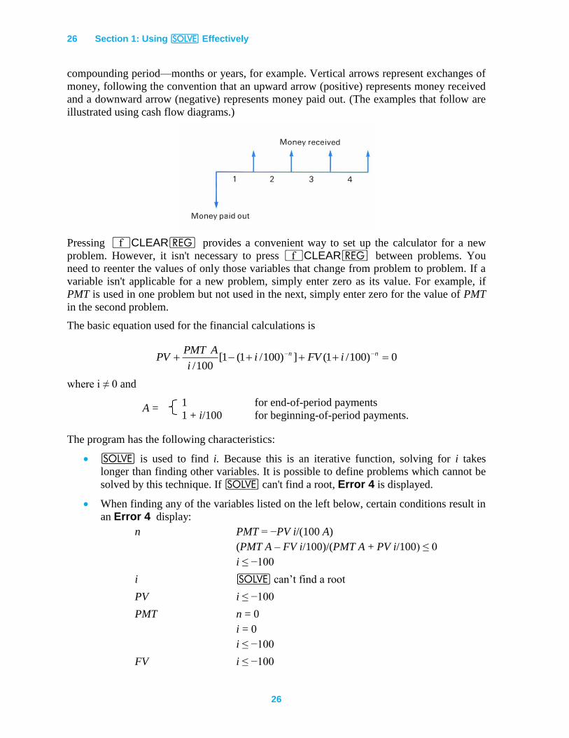
A financial problem can usually be represented by a cash flow diagram. This is a pictorial
representation of the timing and direction of financial transactions. The cash flow diagram
has a horizontal time line that is divided into equal increments that correspond to the
26 Section 1: Using _ Effectively
26
compounding period—months or years, for example. Vertical arrows represent exchanges of
money, following the convention that an upward arrow (positive) represents money received
and a downward arrow (negative) represents money paid out. (The examples that follow are
illustrated using cash flow diagrams.)
Pressing ´CLEARQ provides a convenient way to set up the calculator for a new
problem. However, it isn't necessary to press ´CLEARQ between problems. You
need to reenter the values of only those variables that change from problem to problem. If a
variable isn't applicable for a new problem, simply enter zero as its value. For example, if
PMT is used in one problem but not used in the next, simply enter zero for the value of PMT
in the second problem.
The basic equation used for the financial calculations is
0)100/1(])100/1(1[100/
nn iFVii
APMTPV
where i ≠ 0 and
A = 1 for end-of-period payments
1 + i/100 for beginning-of-period payments.
The program has the following characteristics:
_ is used to find i. Because this is an iterative function, solving for i takes
longer than finding other variables. It is possible to define problems which cannot be
solved by this technique. If _ can't find a root, Error 4 is displayed.
When finding any of the variables listed on the left below, certain conditions result in
an Error 4 display:
n PMT = −PV i/(100 A)
(PMT A – FV i/100)/(PMT A + PV i/100) ≤ 0
i ≤ −100
i _ can’t find a root
PV i ≤ −100
PMT n = 0
i = 0
i ≤ −100
FV i ≤ −100
Section 1: Using _ Effectively 27
If a problem has a specified interest rate of 0, the program generates an Error 0
display (or Error 4 when solving for PMT).
Problems with extremely large (greater than 106) or extremely small (less than 10
−6)
values for n and i may give invalid results:
Interest problems with balloon payments of opposite signs to the periodic payments
may have more than one mathematically correct answer (or no answer at all). This
program may find one of the answers but has no way of finding or indicating other
possibilities.
Keystrokes Display
|¥ Program mode.
´CLEARM 000-
´bA 001-42,21,11 n routine.
O1 002- 44 1 Stores n.
¦ 003- 31
G1 004- 32 1 Calculates n.
|K 005- 43 36
l*0 006-45,20, 0
l5 007- 45 5
® 008- 34
- 009- 30 Calculates
PV – 100 PMT A/i.
|K 010- 43 36
l+3 011-45,40, 3 Calculates PV + 100 PMT A/i.
|~ 012- 43 20 Tests PMT = −PV i/(100 A).
t0 013- 22 0
÷ 014- 10
” 015- 16
|T4 016-43,30, 4 Tests x ≤ 0.
t0 017- 22 0
|N 018- 43 12
l6 019- 45 6
|N 020- 43 12
÷ 021- 10
O1 022- 44 1
|n 023- 43 32
´bB 024-42,21,12 i routine.
O2 025- 44 2 Stores i.
¦ 026- 31
. 027- 48
2 028- 2
28 Section 1: Using _ Effectively
28
Keystrokes Display
v 029- 36
“ 030- 26
” 031- 16
3 032- 3
|"1 033-43, 5, 1 Clears flag 1 for _
subroutine.
´_3 034-42,10, 3
t4 035- 22 4
t0 036- 22 0
´b4 037-42,21, 4
“ 038- 26
2 039- 2
* 040- 20 Calculates i.
O2 041- 44 2
|n 042- 43 32
´bC 043-42,21,13 PV routine.
O3 044- 44 3 Stores PV.
¦ 045- 31
G1 046- 32 1 Calculates PV.
G2 047- 32 2
” 048- 16
O3 049- 44 3
|n 050- 43 32
´bÁ 051-42,21,14 PMT routine.
O4 052- 44 4 Stores PMT.
¦ 053- 31
1 054- 1 Calculates PMT.
O4 055- 44 4
G1 056- 32 1
l3 057- 45 3
G2 058- 32 2
® 059- 34
÷ 060- 10
” 061- 16
O4 062- 44 4
|n 063- 43 32
´bE 064-42,21,15 FV routine.
O5 065- 44 5 Stores FV.
Section 1: Using _ Effectively 29
Keystrokes Display
¦ 066- 31
G1 067- 32 1 Calculates FV.
l+3 068-45,40, 3
l÷7 069-45,10, 7
” 070- 16
O5 071- 44 5
|n 072- 43 32
´b1 073-42,21, 1
|F1 074-43, 4, 1 Sets flag 1 for subroutine 3.
1 075- 1
l2 076- 45 2
|k 077- 43 14 Calculates i/100.
´b3 078-42,21, 3 _ subroutine.
O8 079- 44 8
1 080- 1
O0 081- 44 0
+ 082- 40
|T4 083-43,30, 4 Tests i ≤ 100.
t0 084- 22 0
O6 085- 44 6
|?0 086-43, 6, 0 Tests for end-of-period
payments.
O0 087- 44 0
l1 088- 45 1
” 089- 16
Y 090- 14 Calculates (1 + i/100)−n
.
O7 091- 44 7
1 092- 1
® 093- 34
- 094- 30 Calculates 1 − (1 + i/100)−n
.
|~ 095- 43 20 Tests i = 0 or n = 0.
t0 096- 22 0
l*0 097-45,20, 0
l4 098- 45 4
l÷8 099-45,10, 8
* 100- 20
|?1 101-43, 6, 1 Tests flag 1 set.
|n 102- 43 32
30 Section 1: Using _ Effectively
30
Keystrokes Display
l+3 103-45,40, 3 _ subroutine continues.
´b2 104-42,21, 2
l5 105- 45 5
l*7 106-45,20, 7 Calculates FV(1 + i/100)−n
.
+ 107- 40
|n 108- 43 32 _ subroutine ends.
Labels used: A, B, C, D, E, 0, 1, 2, 3, and 4.
Registers used: R0 (A), R1 (n), R2 (i), R3 (PV), R4 (PMT), R5 (FV), R6, R7, and R8.
To use the program:
1. Press 8´m% to reserve R0 through R8.
2. Press ´U to activate User mode.
3. If necessary, press ´CLEARQ to clear all of the financial variables. You don't
need to clear the registers if you intend to specify all of the values.
4. Set flag 0 according to how payments are to be figured:
Press |"0 for payments at the end of the period.
Press |F0 for payments at the beginning of the period.
5. Enter the known values of the financial variables:
To enter n, key in the value and press A.
To enter i, key in the value and press B.
To enter PV, key in the value and press C.
To enter PMT, key in the value and press Á.
To enter FV, key in the value and press E.
6. Calculate the unknown value:
To calculate n, press A ¦.
To calculate i, press B ¦.
To calculate PV, press C ¦.
To calculate PMT, press Á ¦.
To calculate FV, press E ¦.
7. To solve another problem, repeat steps 3 through 6 as needed. Be sure that any variable
not to be used in the problem has a value of zero.
Section 1: Using _ Effectively 31
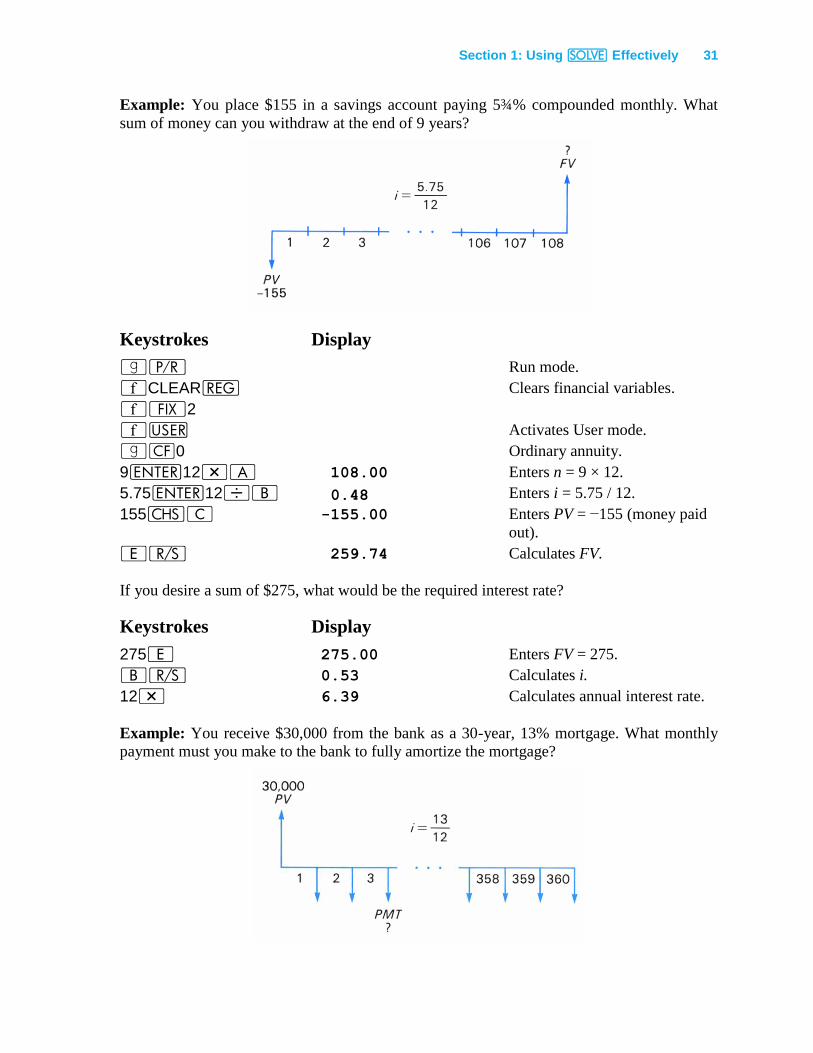
Example: You place $155 in a savings account paying 5¾% compounded monthly. What
sum of money can you withdraw at the end of 9 years?
Keystrokes Display
|¥ Run mode.
´CLEARQ Clears financial variables.
´•2
´U Activates User mode.
|"0 Ordinary annuity.
9v12*A 108.00 Enters n = 9 × 12.
5.75v12÷B 0.48 Enters i = 5.75 / 12.
155”C -155.00 Enters PV = −155 (money paid
out).
E¦ 259.74 Calculates FV.
If you desire a sum of $275, what would be the required interest rate?
Keystrokes Display
275E 275.00 Enters FV = 275.
B¦ 0.53 Calculates i.
12* 6.39 Calculates annual interest rate.
Example: You receive $30,000 from the bank as a 30-year, 13% mortgage. What monthly
payment must you make to the bank to fully amortize the mortgage?
32 Section 1: Using _ Effectively
32
Keystrokes Display
´CLEARQ Clears financial variables
30v12*A 360.00 Enters n = 30 × 12.
13v12÷B 1.08 Enters i = 13/12.
30000C 30,000.00 Enters PV = 30,000.
Á¦ -331.86 Calculates PMT (money paid out).
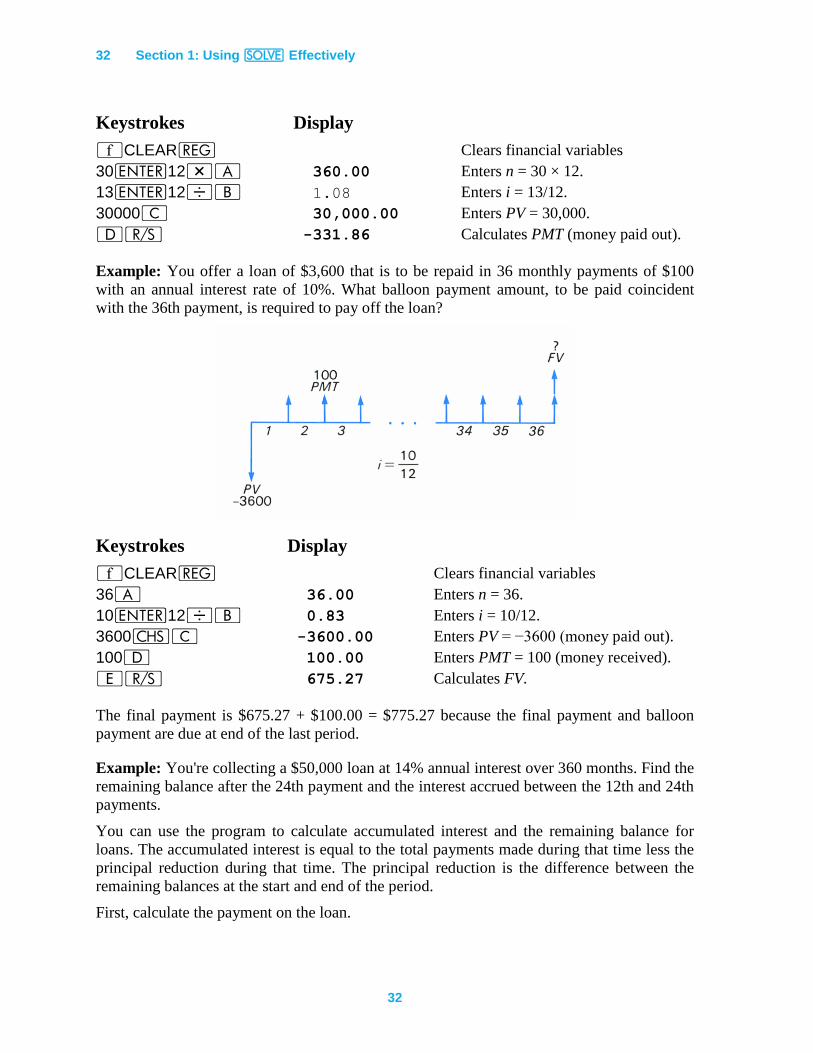
Example: You offer a loan of $3,600 that is to be repaid in 36 monthly payments of $100
with an annual interest rate of 10%. What balloon payment amount, to be paid coincident
with the 36th payment, is required to pay off the loan?
Keystrokes Display
´CLEARQ Clears financial variables
36A 36.00 Enters n = 36.
10v12÷B 0.83 Enters i = 10/12.
3600”C -3600.00 Enters PV = −3600 (money paid out).
100Á 100.00 Enters PMT = 100 (money received).
E¦ 675.27 Calculates FV.
The final payment is $675.27 + $100.00 = $775.27 because the final payment and balloon
payment are due at end of the last period.
Example: You're collecting a $50,000 loan at 14% annual interest over 360 months. Find the
remaining balance after the 24th payment and the interest accrued between the 12th and 24th
payments.
You can use the program to calculate accumulated interest and the remaining balance for
loans. The accumulated interest is equal to the total payments made during that time less the
principal reduction during that time. The principal reduction is the difference between the
remaining balances at the start and end of the period.
First, calculate the payment on the loan.
Section 1: Using _ Effectively 33
Keystrokes Display
´CLEARQ Clears financial variables
360A 360.00 Enters n = 360.
14v12÷B 1.17 Enters i = 14/12.
50000”C -50,000.00 Enters PV = −50,000.
Á¦ 592.44 Calculates PMT.
Now calculate the remaining balance at month 24.
Keystrokes Display
24A 24.00 Enters n = 24.
E¦ 49,749.56 Calculates FV at month 24.
Store this remaining balance, then calculate the remaining balance at month 12 and the
principal reduction between payments 12 and 24.
Keystrokes Display
OV 49,749.56
12A 12.00 Enters n = 12.
E¦ 49,883.48 Calculates FV at month 12.
lV 49,749.56 Recalls FV at month 24.
- 133.92 Calculates principal reduction.
The accrued interest is the value of 12 payments less the principal reduction.
Keystrokes Display
l4 592.44 Recalls PMT.
12* 7,109.23 Calculates value of payments.
®- 6,975.31 Calculates accrued interest.
Example: A leasing firm is considering the purchase of a minicomputer for $63,000 and
wants to achieve a 13% annual yield by leasing the computer for a 5-year period. At the end
of the lease the firm expects to sell the computer for at least $10,000. What monthly payment
should the firm charge in order to achieve a 13% yield? (Because the lease payments are due
at the beginning of each month, be sure to set flag 0 to specify beginning-of-period
payments.)
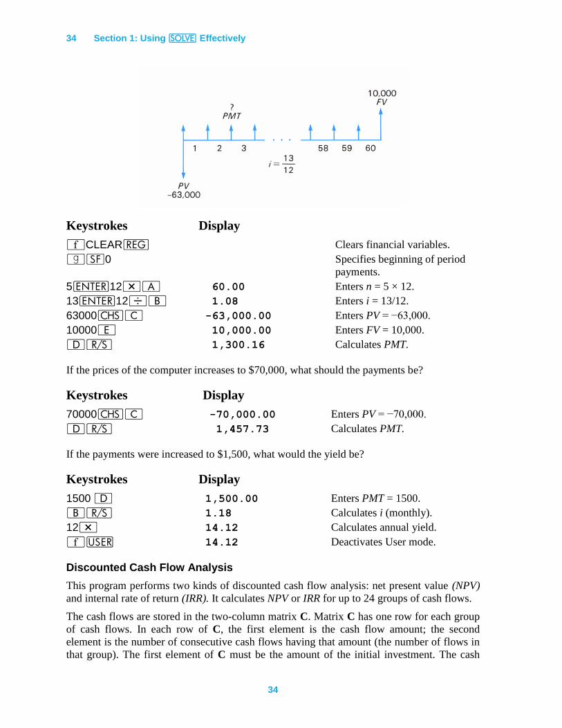
34 Section 1: Using _ Effectively
34
Keystrokes Display
´CLEARQ Clears financial variables.
|F0 Specifies beginning of period
payments.
5v12*A 60.00 Enters n = 5 × 12.
13v12÷B 1.08 Enters i = 13/12.
63000”C -63,000.00 Enters PV = −63,000.
10000E 10,000.00 Enters FV = 10,000.
Á¦ 1,300.16 Calculates PMT.
If the prices of the computer increases to $70,000, what should the payments be?
Keystrokes Display
70000”C -70,000.00 Enters PV = −70,000.
Á¦ 1,457.73 Calculates PMT.
If the payments were increased to $1,500, what would the yield be?
Keystrokes Display
1500 Á 1,500.00 Enters PMT = 1500.
B¦ 1.18 Calculates i (monthly).
12* 14.12 Calculates annual yield.
´U 14.12 Deactivates User mode.
Discounted Cash Flow Analysis
This program performs two kinds of discounted cash flow analysis: net present value (NPV)
and internal rate of return (IRR). It calculates NPV or IRR for up to 24 groups of cash flows.
The cash flows are stored in the two-column matrix C. Matrix C has one row for each group
of cash flows. In each row of C, the first element is the cash flow amount; the second
element is the number of consecutive cash flows having that amount (the number of flows in
that group). The first element of C must be the amount of the initial investment. The cash
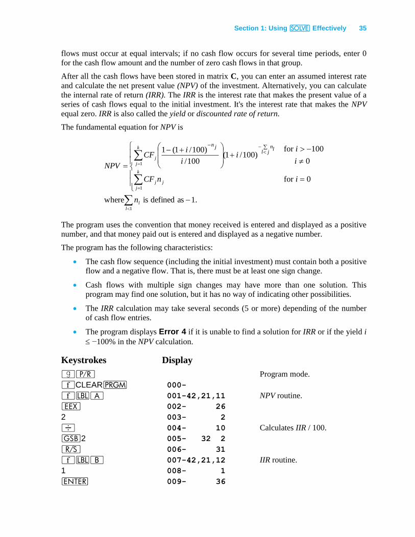
Section 1: Using _ Effectively 35
flows must occur at equal intervals; if no cash flow occurs for several time periods, enter 0
for the cash flow amount and the number of zero cash flows in that group.
After all the cash flows have been stored in matrix C, you can enter an assumed interest rate
and calculate the net present value (NPV) of the investment. Alternatively, you can calculate
the internal rate of return (IRR). The IRR is the interest rate that makes the present value of a
series of cash flows equal to the initial investment. It's the interest rate that makes the NPV
equal zero. IRR is also called the yield or discounted rate of return.
The fundamental equation for NPV is
1
1
1
.1asdefinediswhere
0for
0
100for)100/1(
100/
)100/1(1
l
l
k
j
jj
k
j
j
n
inCF
i
ii
i
iCF
NPV
jllnjn
The program uses the convention that money received is entered and displayed as a positive
number, and that money paid out is entered and displayed as a negative number.
The program has the following characteristics:
The cash flow sequence (including the initial investment) must contain both a positive
flow and a negative flow. That is, there must be at least one sign change.
Cash flows with multiple sign changes may have more than one solution. This
program may find one solution, but it has no way of indicating other possibilities.
The IRR calculation may take several seconds (5 or more) depending of the number
of cash flow entries.
The program displays Error 4 if it is unable to find a solution for IRR or if the yield i
−100% in the NPV calculation.
Keystrokes Display
|¥ Program mode.
´CLEARM 000-
´bA 001-42,21,11 NPV routine.
“ 002- 26
2 003- 2
÷ 004- 10 Calculates IIR / 100.
G2 005- 32 2
¦ 006- 31
´bB 007-42,21,12 IIR routine.
1 008- 1
v 009- 36
36 Section 1: Using _ Effectively
36
Keystrokes Display
“ 010- 26
” 011- 16
3 012- 3
´_2 013-42,10, 2
t1 014- 22 1
t0 015- 22 0 Branch for no IRR solution.
´b1 016-42,21, 1
“ 017- 26
2 018- 2
* 019- 20
¦ 020- 31
´b2 021-42,21, 2 Calculates NPV.
|"0 022-43, 5, 0
O2 023- 44 2
1 024- 1
O4 025- 44 4
+ 026- 40 Calculates 1 + IRR / 100.
|T4 027-43,30, 4 Tests IRR ≤ −100.
t0 028- 22 0 Branch for IRR ≤ −100.
O3 029- 44 3
0 030- 0
O5 031- 44 5
´>1 032-42,16, 1
´b3 033-42,21, 3
|?0 034-43, 6, 0 Tests if all flows used.
t7 035- 22 7 Branch for all flows used.
G6 036- 32 6
l2 037- 45 2
|~ 038- 43 20 Tests IRR = 0;
t4 039- 22 4 Branch for IRR = 0.
1 040- 1
+ 041- 40
G6 042- 32 6
” 043- 16
Y 044- 14
O4 045- 44 4
1 046- 1
® 047- 34
Section 1: Using _ Effectively 37
Keystrokes Display
- 048- 30
l÷2 049-45,10, 2
l*3 050-45,20, 3
t5 051- 22 5
´b4 052-42,21, 4
® 053- 34
G6 054- 32 6
´b5 055-42,21, 5
* 056- 20
O+5 057-44,40, 5
l4 058- 45 4
O*3 059-44,20, 3
t3 060- 22 3
´b6 061-42,21, 6 Recalls cash flow element.
´UlC 062u 45 13
´U
|n 063- 43 32
| F0 064-43, 4, 0 Sets flag 0 if last element.
|n 065- 43 32
´b7 066-42,21, 7
l5 067- 45 5 Recalls NPV.
|n 068- 43 32
Labels used: A, B, and 0 through 7.
Registers used: R0 through R5.
Matrix used: C.
To use the discounted cash flow analysis program:
1. Press 5´m% to allocate registers R0 through R5.
2. Press ´U to activate User mode (unless it's already active).
3. Key in the number of cash flow groups, then press v2´mC to dimension matrix C.
4. Press ´>1 to set the row and column numbers to 1.
5. For each cash flow group:
a. Key in the amount and press OC, then
b. Key in the number of occurrences and press OC.
6. Calculate the desired parameter:
To calculate IRR, press B.
38 Section 1: Using _ Effectively
38
To calculate NPV, enter periodic interest rate i in percent and press A. Repeat
for as many interest rates as needed.
7. Repeat steps 3 through 6 for other sets of cash flows.
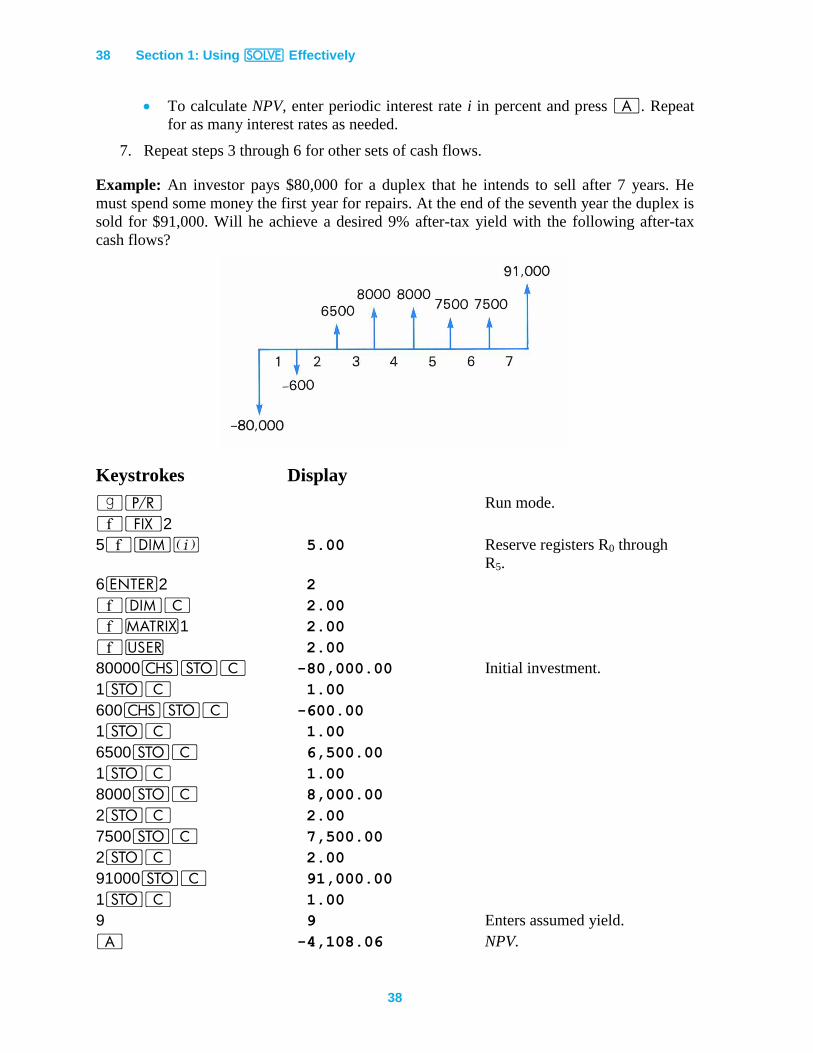
Example: An investor pays $80,000 for a duplex that he intends to sell after 7 years. He
must spend some money the first year for repairs. At the end of the seventh year the duplex is
sold for $91,000. Will he achieve a desired 9% after-tax yield with the following after-tax
cash flows?
Keystrokes Display
|¥ Run mode.
´•2
5´m% 5.00 Reserve registers R0 through
R5.
6v2 2
´mC 2.00
´>1 2.00
´U 2.00
80000”OC -80,000.00 Initial investment.
1OC 1.00
600”OC -600.00
1OC 1.00
6500OC 6,500.00
1OC 1.00
8000OC 8,000.00
2OC 2.00
7500OC 7,500.00
2OC 2.00
91000OC 91,000.00
1OC 1.00
9 9 Enters assumed yield.
A -4,108.06 NPV.
Section 1: Using _ Effectively 39
Since the NPV is negative, the investment does not achieve the desired 9% yield. Calculate
the IRR.
Keystrokes Display
B 8.04 IRR (after about 5 seconds).
The IRR is less than the desired 9% yield.
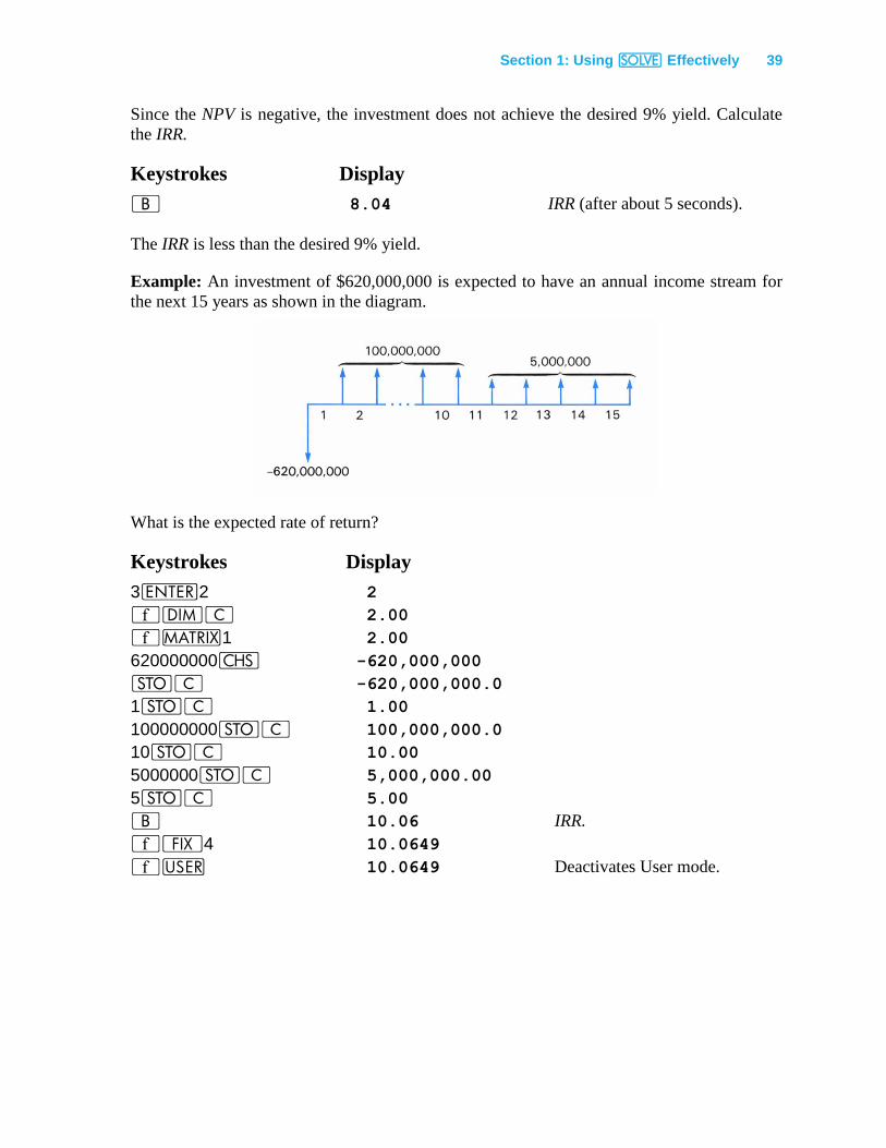
Example: An investment of $620,000,000 is expected to have an annual income stream for
the next 15 years as shown in the diagram.
What is the expected rate of return?
Keystrokes Display
3v2 2
´mC 2.00
´>1 2.00
620000000” -620,000,000
OC -620,000,000.0
1OC 1.00
100000000OC 100,000,000.0
10OC 10.00
5000000OC 5,000,000.00
5OC 5.00
B 10.06 IRR.
´•4 10.0649
´U 10.0649 Deactivates User mode.
40
Section 2: Working with f
The HP-15C gives you the ability to perform numerical integration using f. This section
shows you how to use f effectively and describes techniques that enable you to handle
difficult integrals.
Numerical Integration Using f A calculator using numerical integration can almost never calculate an integral precisely. But
the f function asks you in a convenient way to specify how much error is tolerable. It asks
you to set the display format according to how many figures are accurate in the integrand
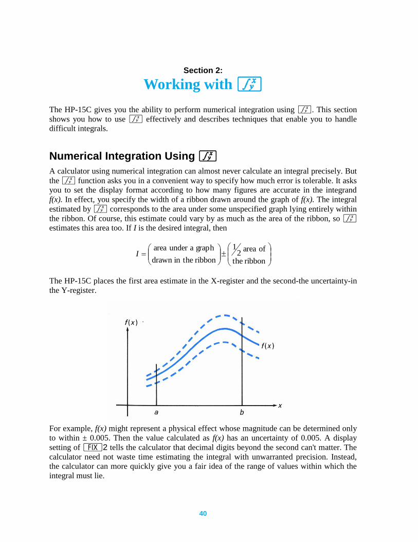
f(x). In effect, you specify the width of a ribbon drawn around the graph of f(x). The integral
estimated by f corresponds to the area under some unspecified graph lying entirely within
the ribbon. Of course, this estimate could vary by as much as the area of the ribbon, so f
estimates this area too. If I is the desired integral, then
ribbonthe
ofarea2
1
ribbontheindrawn
graphaunderareaI
The HP-15C places the first area estimate in the X-register and the second-the uncertainty-in
the Y-register.
For example, f(x) might represent a physical effect whose magnitude can be determined only
to within ± 0.005. Then the value calculated as f(x) has an uncertainty of 0.005. A display
setting of •2 tells the calculator that decimal digits beyond the second can't matter. The
calculator need not waste time estimating the integral with unwarranted precision. Instead,
the calculator can more quickly give you a fair idea of the range of values within which the
integral must lie.
Section 2: Working with f 41
The HP-15C doesn't prevent you from declaring that f(x) is far more accurate than it really is.
You can specify the display setting after a careful error analysis, or you can just offer a
guess. You may leave the display set to i or • 4 without much further thought. You
will get an estimate of the integral and its uncertainty, enabling you to interpret the result
more intelligently than if you got the answer with no idea of its accuracy or inaccuracy.
The f algorithm uses a Romberg method for accumulating the value of the integral.
Several refinements make it more effective.
Instead of using uniformly spaced samples, which can induce a kind of resonance or aliasing
that produces misleading results when the integrand is periodic f uses samples that are
spaced nonuniformly. Their spacing can be demonstrated by substituting, say,
3
2
1
2
3uux
into
1
1
231
1)1(
2
3
2
1
2
3)( duuuufdxxfI
and sampling u uniformly. Besides suppressing resonance, the substitution has two more
benefits. First, no sample need be drawn from either end of the interval of integration (except
when the interval is so narrow that no other possibilities are available). As a result, an
integral like
3
0
sindx
x
x
won't be interrupted by division by zero at an endpoint. Second, f can integrate functions
that behave like ax whose slope is infinite at an endpoint. Such functions are encountered
when calculating the area enclosed by a smooth, closed curve.
Another refinement is that f uses extended precision, 13 significant digits, to accumulate
the internal sums. This allows thousands of samples to be accumulated, if necessary, without
losing to roundoff any more information than is lost within your function subroutine.
Accuracy of the Function to be Integrated
The accuracy of an integral calculated using f depends on the accuracy of the function
calculated by your subroutine. This accuracy, which you specify using the display format,
depends primarily on three considerations:
The accuracy of empirical constants in the function.
The degree to which the function may accurately describe a physical situation.
The extent of round-off error in the internal calculations of the calculator.
42 Section 2: Working with f
42
Functions Related to Physical Situations
Functions like cos(4 - sin) are pure mathematical functions. In this context, this means that
the functions do not contain any empirical constants, and neither the variables nor the limits
of integration represent actual physical quantities. For such functions, you can specify as
many digits as you want in the display format (up to nine) to achieve the desired degree of
accuracy in the integral.† All you need to consider is the trade-off between the accuracy and
calculation time.
There are additional considerations, however, when you're integrating functions relating to an
actual physical situation. Basically, with such functions you should ask yourself whether the
accuracy you would like in the integral is justified by the accuracy in the function. For
example, if the function contains empirical constants that are specified to only, say, three
significant digits, it might not make sense to specify more than three digits in the display
format.
Another important consideration—and one which is more subtle and therefore more easily
overlooked—is that nearly every function relating to a physical situation is inherently
inaccurate to a certain degree, because it is only a mathematical model of an actual process
or event. A mathematical model is itself an approximation that ignores the effects of known
or unknown factors which are insignificant to the degree that the results are still useful.
An example of a mathematical model is the normal distribution function,
t
dxe
x
2
22/2)(
which has been found to be useful in deriving information concerning physical measurements
on living organisms, product dimensions, average temperatures, etc. Such mathematical
descriptions typically are either derived from theoretical considerations or inferred from
experimental data. To be practically useful, they are constructed with certain assumptions,
such as ignoring the effects of relatively insignificant factors. For example, the accuracy of
results obtained using the normal distribution function as a model of the distribution of
certain quantities depends on the size of the population being studied. And the accuracy of
results obtained from the equation s = s0 − ½gt2, which gives the height of a falling body,
ignores the variation with altitude of g, the acceleration of gravity.
Thus, mathematical descriptions of the physical world can provide results of only limited
accuracy. If you calculated an integral with an apparent accuracy beyond that with which the
model describes the actual behavior of the process or event, you would not be justified in
using the calculated value to the full apparent accuracy.
Round-Off Error in Internal Calculations
With any computational device—including the HP-15C—calculated results must be
“rounded off” to a finite number of digits (10 digits in the HP-15C). Because of this round-
off error, calculated results—especially results of evaluating a function that contains several
† Provided that f(x) is still calculated accurately, despite round-off error, to the number of digits shown in the display.
Section 2: Working with f 43
mathematical operations—may not be accurate to all 10 digits that can be displayed. Note
that round-off error affects the evaluation of any mathematical expression, not just the
evaluation of a function to be integrated using f. (Refer to the appendix for additional
information.)
If f(x) is a function relating to a physical situation, its inaccuracy due to round-off typically is
insignificant compared to the inaccuracy due to empirical constants, etc. If f(x) is what we
have called a pure mathematical function, its accuracy is limited only by round-off error.
Generally, it would require a complicated analysis to determine precisely how many digits of
a calculated function might be affected by round-off. In practice, its effects are typically (and
adequately) determined through experience rather than analysis.
In certain situations, round-off error can cause peculiar results, particularly if you should
compare the results of calculating integrals that are equivalent mathematically but differ by a
transformation of variables. However, you are unlikely to encounter such situations in typical
applications.
Shortening Calculation Time
The time required for f to calculate an integral depends on how soon a certain density of
sample points is achieved in the region where the function is interesting. The calculation of
the integral of any function will be prolonged if the interval of integration includes mostly
regions where the function is not interesting. Fortunately, if you must calculate such an
integral, you can modify the problem so that the calculation time is reduced. Two such
techniques are subdividing the interval of integration and transformation of variables.
Subdividing the Interval of Integration
In regions where the slope of f(x) is varying appreciably, a high density of sample points is
necessary to provide an approximation that changes insignificantly from one iteration to the
next. However, in regions where the slope of the function stays nearly constant, a high
density of sample points is not necessary. This is because evaluating the function at
additional sample points would not yield much new information about the function, so it
would not dramatically affect the disparity between successive approximations.
Consequently, in such regions an approximation of comparable accuracy could be achieved
with substantially fewer sample points: so much of the time spent evaluating the function in
these regions is wasted. When integrating such functions, you can save time by using the
following procedure:
1. Divide the interval of integration into subintervals over which the function is
interesting and subintervals over which the function is uninteresting.
2. Over the subintervals where the function is interesting, calculate the integral in the
display format corresponding to the accuracy you would like overall.
3. Over the subintervals where the function either is not interesting or contributes
negligibly to the integral, calculate the integral with less accuracy, that is, in a display
format specifying fewer digits.
44 Section 2: Working with f
44
4. To get the integral over the entire interval of integration, add together the
approximations and their uncertainties from the integrals calculated over each
subinterval. You can do this easily using the z key.
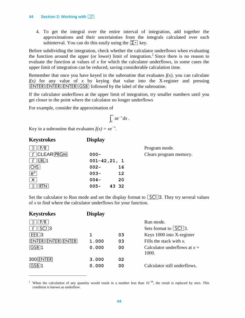
Before subdividing the integration, check whether the calculator underflows when evaluating
the function around the upper (or lower) limit of integration.‡ Since there is no reason to
evaluate the function at values of x for which the calculator underflows, in some cases the
upper limit of integration can be reduced, saving considerable calculation time.
Remember that once you have keyed in the subroutine that evaluates f(x), you can calculate
f(x) for any value of x by keying that value into the X-register and pressing
vvvG followed by the label of the subroutine.
If the calculator underflows at the upper limit of integration, try smaller numbers until you
get closer to the point where the calculator no longer underflows
For example, consider the approximation of
0dxxe x .
Key in a subroutine that evaluates f(x) = xe−x
.
Keystrokes Display
|¥ Program mode.
´CLEARM 000- Clears program memory.
´b1 001-42,21, 1
” 002- 16
' 003- 12
* 004- 20
|n 005- 43 32
Set the calculator to Run mode and set the display format to i3. They try several values
of x to find where the calculator underflows for your function.
Keystrokes Display
|¥ Run mode.
´i3 Sets format to i3.
“3 1 03 Keys 1000 into X-register
vvv 1.000 03 Fills the stack with x.
G1 0.000 00 Calculator underflows at x =
1000.
300v 3.000 02
G1 0.000 00 Calculator still underflows.
‡ When the calculation of any quantity would result in a number less than 10−99, the result is replaced by zero. This
condition is known as underflow.
Section 2: Working with f 45
Keystrokes Display
200v 2.000 00 Try a smaller value of x.
vv 2.000 02
G1 2.768 -85 Calculator doesn’t underflow at
x = 200; try a number between
200 and 250.
225v 2.250 02
vv 2.250 02
G1 4.324 -96 Calculator is close to underflow.
At this point, you can use _ to pinpoint the smallest value of x at which the calculator
underflows.
Keystrokes Display
) 2.250 02 Roll down stack until the last
value tried is in the X- and Y-
registers.
´_1 2.280 02 The minimum value of x at
which the calculator underflows
is about 228.
You've now determined that you need integrate only from 0 to 228. Since the integrand is
interesting only for values of x less than 10, divide the interval of integration there. The
problem has now become:
228
0
10
0
228
100dxxedxxedxxedxxe xxxx
.
Keystrokes Display
7´m% 7.000 00 Allocates statistical storage
registers.
´CLEARz 0.000 00 Clears statistical storage
registers.
0v 0.000 00 Keys in lower limit of
integration over first subinterval.
10 10 Keys in upper limit of
integration over first subinterval.
´f1 9.995 -01 Integral over (0,10) calculated in
i3.
z 1.000 00 Sum approximation and its
uncertainty in registers R3 and
R5.
46 Section 2: Working with f
46
Keystrokes Display
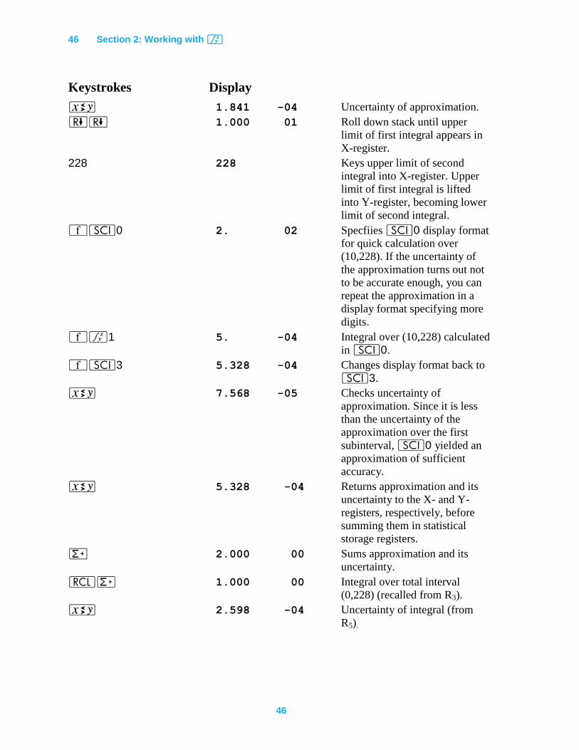
® 1.841 -04 Uncertainty of approximation.
)) 1.000 01 Roll down stack until upper
limit of first integral appears in
X-register.
228 228 Keys upper limit of second
integral into X-register. Upper
limit of first integral is lifted
into Y-register, becoming lower
limit of second integral.
´i0 2. 02 Specfiies i0 display format
for quick calculation over
(10,228). If the uncertainty of
the approximation turns out not
to be accurate enough, you can
repeat the approximation in a
display format specifying more
digits.
´f1 5. -04 Integral over (10,228) calculated
in i0.
´i3 5.328 -04 Changes display format back to
i3.
® 7.568 -05 Checks uncertainty of
approximation. Since it is less
than the uncertainty of the
approximation over the first
subinterval, i0 yielded an
approximation of sufficient
accuracy.
® 5.328 -04 Returns approximation and its
uncertainty to the X- and Y-
registers, respectively, before
summing them in statistical
storage registers.
z 2.000 00 Sums approximation and its
uncertainty.
lz 1.000 00 Integral over total interval
(0,228) (recalled from R3).
® 2.598 -04 Uncertainty of integral (from
R5).
Section 2: Working with f 47
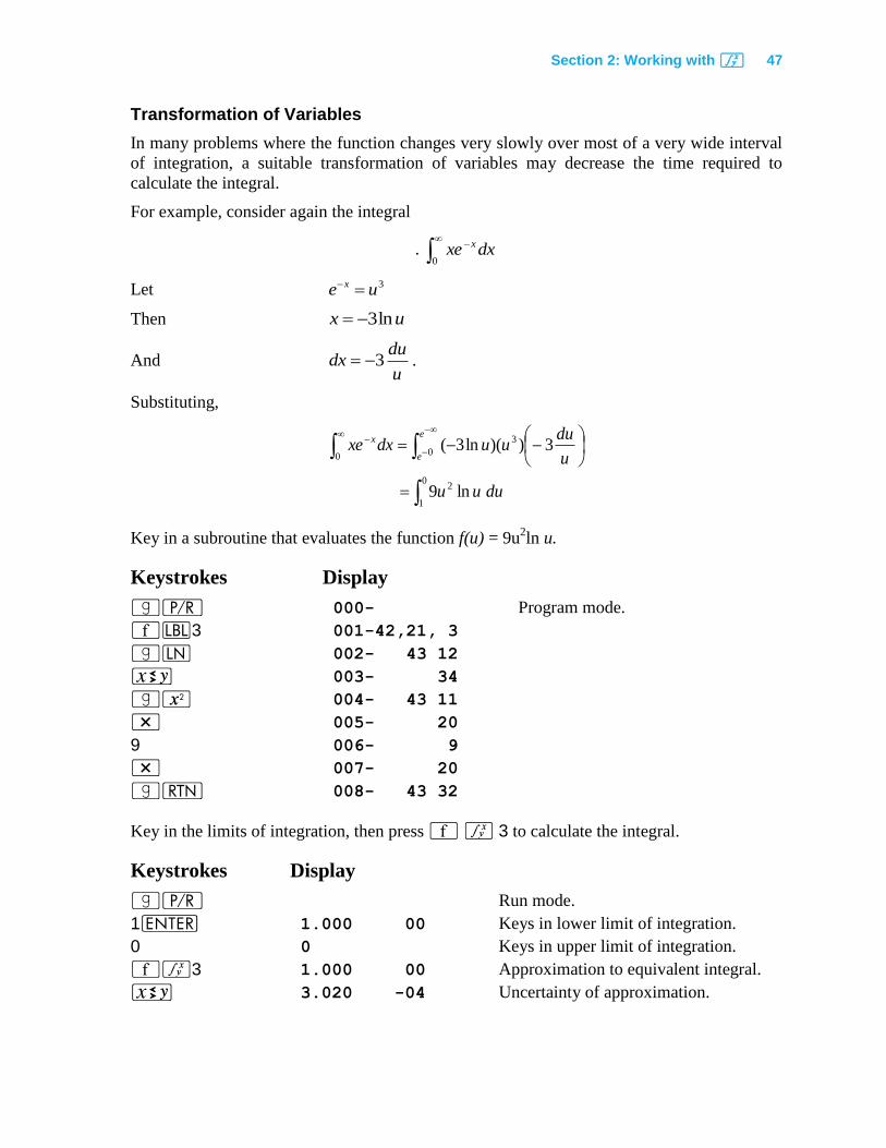
Transformation of Variables
In many problems where the function changes very slowly over most of a very wide interval
of integration, a suitable transformation of variables may decrease the time required to
calculate the integral.
For example, consider again the integral
.
0dxxe x
Let 3ue x
Then ux ln3
And u
dudx 3 .
Substituting,
0
1
2
0 0
3
ln9
3))(ln3(
duuu
u
duuudxxe
e
e
x
Key in a subroutine that evaluates the function f(u) = 9u2ln u.
Keystrokes Display
|¥ 000- Program mode.
´b3 001-42,21, 3
|N 002- 43 12
® 003- 34
|x 004- 43 11
* 005- 20
9 006- 9
* 007- 20
|n 008- 43 32
Key in the limits of integration, then press ´ f 3 to calculate the integral.
Keystrokes Display
|¥ Run mode.
1v 1.000 00 Keys in lower limit of integration.
0 0 Keys in upper limit of integration.
´f3 1.000 00 Approximation to equivalent integral.
® 3.020 -04 Uncertainty of approximation.
48 Section 2: Working with f
48
The approximation agrees with the value calculated In the previous problem for the same
integral.
Evaluating Difficult Integrals
Certain conditions can prolong the time required to evaluate an integral or can cause
inaccurate results. As discussed in the HP-15C Owner's Handbook, these conditions are
related to the nature of the integrand over the interval of integration.
One class of integrals that are difficult to calculate is improper integrals. An improper
integral is one that involves ∞ in at least one of the following ways:
One or both limits of integration are ±∞, such as
due u2
.
The integrand tends to ±∞ someplace in the range of integration, such as
1)ln(1
0 duu .
The integrand oscillates infinitely rapidly somewhere in the range of integration,
such as
½)cos(ln1
0 duu .
Equally troublesome are nearly improper integrals, which are characterized by
The integrand or its first derivative or its first derivative changes wildly within a
relatively narrow subinterval of the range of integration, or oscillates frequently
across that range.
The HP-15C attempts to deal with certain of the second type of improper integral by usually
not sampling the integrand at the limits of integration.
Because improper and nearly improper integrals are not uncommon in practice, you should
recognize them and take measures to evaluate them accurately. The following examples
illustrate techniques that are helpful.
Consider the integrand
2
2 )cos(ln2)(
x
xxf
.
This function loses its accuracy when x becomes small. This is caused by rounding cos(x2) to
1, which drops information about how small x is. But by using u = cos(x2), you can evaluate
the integrand as
.1ifcos
ln2
1if1
)(1
uu
u
u
xf
Section 2: Working with f 49
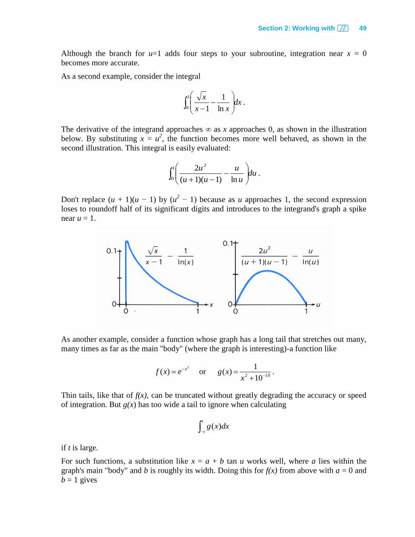
Although the branch for u=1 adds four steps to your subroutine, integration near x = 0
becomes more accurate.
As a second example, consider the integral
1
0 ln
1
1dx
xx
x.
The derivative of the integrand approaches ∞ as x approaches 0, as shown in the illustration
below. By substituting x = u2, the function becomes more well behaved, as shown in the
second illustration. This integral is easily evaluated:
1
0
2
ln)1)(1(
2du
u
u
uu
u.
Don't replace (u + 1)(u − 1) by (u2 − 1) because as u approaches 1, the second expression
loses to roundoff half of its significant digits and introduces to the integrand's graph a spike
near u = 1.
As another example, consider a function whose graph has a long tail that stretches out many,
many times as far as the main "body" (where the graph is interesting)-a function like
2
)( xexf or 102 10
1)(
xxg .
Thin tails, like that of f(x), can be truncated without greatly degrading the accuracy or speed
of integration. But g(x) has too wide a tail to ignore when calculating
t
tdxxg )(
if t is large.
For such functions, a substitution like x = a + b tan u works well, where a lies within the
graph's main "body" and b is roughly its width. Doing this for f(x) from above with a = 0 and
b = 1 gives
50 Section 2: Working with f
50
t
ut
duuedxxf1tan
0
2tan
0)tan1()(
2
,
which is calculated readily even with t as large as 1010
. Using the same substitution with g(x),
values near a = 0 and b = 10−5
provide good results.
This example involves subdividing the interval of integration. Although a function may have
features that look extreme over the entire interval of integration, over portions of that interval
the function may look more well-behaved. Subdividing the interval of integration works best
when combined with appropriate substitutions. Consider the integral
.)1/()1(1
)1/()(1
)1/()1(
)1/()1/(
)1/()1/()1/(
1
0
88/554/18
1
1
0
646462
1
0
6462
1
0
64621
0
64
1
641
0
64
0
64
vdvvv
xdxxx
xdxx
uduuxdx
xdxxdxxdx
These steps use the substitutions x = 1/ u and x = v1/8
and some algebraic manipulation.
Although the original integral is improper, the last integral is easily handled by f. In fact,
by separating the constant term from the integral, you obtain (using i8) an answer with
13 significant digits:
1.000401708155 ± 1.2 × 10⁻¹²
.
A final example drawn from real life involves the electrostatic field about an ellipsoidal
probe with principal semiaxes a, b, and c:
0 2222 ))()(()( xcxbxaxa
dxV
for a=100, b =2, and c= 1.§
Transform this improper integral to a proper one by substituting x = (a2 − c
2)/(1 − u
2) − a
2:
1
22 )/()1(r
duquupV
where
62222 1000060018.2))((/2 bacap
32222 10001200480.3)(/)( bacbq
§ From Stratton, J.A., Electromagnetic Theory, McGraw-Hill, New York, 1941, pp.201-217.
Section 2: Working with f 51
01.0/ acr
However, this integral is nearly improper because q and r are both so nearly zero. But by
using an integral in closed form that sufficiently resembles the troublesome part of V, the
difficulty can be avoided. Try
.1084018188070.8
))/()11ln((
)ln(/
6
2
121 2
qrrqp
quupqudupWrr
Then
.)11(1
/
)/1)/()1((
1
22
2
1222
duquu
u
r
pWp
duququupWV
r
r
The HP-15C readily handles this integral. Don't worry about 21 u as u approaches 1
because the figures lost to roundoff aren't needed.
Application
The following program calculates the values of four special functions for any argument x:
dtex t 2/2
2
1)(P
(normal distribution function)
x
t dtexPx 2/2
2
1)(1)(Q
(complementary normal distribution function)
xt dtex
0
22)(erf
(error function)
x
t dtexx22
)(erf1)(erfc
(complementary error function)
The program calculates these functions using the transformation 2teu whenever |x| > 1.6.
The function value is returned in the X-register, and the uncertainty of the integral is returned
in the Y-register. (The uncertainty of the function value is approximately the same order of
magnitude as the number in the Y-register.) The original argument is available in register R0.
52 Section 2: Working with f
52
The program has the following characteristics:
The display format specifies the accuracy of the integrand in the same way as it does
for f itself. However, if you specify an unnecessarily large number of display
digits, the calculation will be prolonged.
Small function values, such as Q(20), P(−20), and erfc(10), are accurately computed
as quickly as moderate values.
Keystrokes Display
|¥ Program mode.
´CLEARM 000-
´bA 001-42,21,11 Program for P(x).
O2 002- 44 2 Stores x in R2.
” 003- 16 Calculates −x.
t2 004- 22 2 Branches to calculate P(x) = Q(−x).
´bB 005-42,21,12 Program for Q(x).
O2 006- 44 2 Stores x in R2.
´b2 007-42,21, 2
2 008- 2
¤ 009- 11
÷ 010- 10
GC 011- 32 13 Calculates erfc( 2/x ).
2 012- 2
÷ 013- 10 Calculates
Q(x) = ½ erfc( 2/x )
l2 014- 45 2
O0 015- 44 0 Stores x in R0.
) 016- 33
|n 017- 43 32 Returns function value.
´bC 018-42,21,13 Program for erfc(x).
1 019- 1
G4 020- 32 4
|?1 021-43, 6, 1 Tests flag 1 set.
t5 022- 22 5 Branches for flag 1 set.
1 023- 1
- 024- 30 Calculates erf(x) – 1 for flag 1 clear.
´b5 025-42,21, 5
” 026- 16 Calculates erfc(x).
|n 027- 43 32 Returns function value.
´bE 028-42,21,15 Program for erf(x).
0 029- 0
Section 2: Working with f 53
Keystrokes Display
´b4 030-42,21, 4 Subroutine for erf(x) or erfc(x).
|"1 031-43, 5, 1 Clears flag 1.
O1 032- 44 1 Stores 0 for erf(x), 1 for erfc(x)
® 033- 34
O0 034- 44 0
|a 035- 43 16 Calculates |x|.
1 036- 1
. 037- 48
6 038- 6
|T8 039-43,30, 8 Tests |x|>1.6.
t6 040- 22 6 Branch for |x|>1.6.
0 041- 0
l0 042- 45 0 Recalls x.
´f0 043-42,20, 0 Integrates 2te from 0 to x.
2 044- 2
* 045- 20
´b3 046-42,21, 3 Subroutine to divide by .
|$ 047- 43,26
¤ 048- 11
÷ 049- 10
|n 050- 43 32
´b6 051-42,21, 6 Subroutine to integrate when |x| >
1.6.
|F1 052-43, 4, 1 Sets flag 1.
0 053- 0
l0 054- 45 0
|x 055- 43 11
” 056- 16
' 057- 12 Calculates 2xe .
´f1 058-42,20, 1 Integrates (-ln u)-1/2
from 0 to 2xe
G3 059- 32 3 Divides integral by .
l0 060- 45 0
v 061- 36
|a 062- 43 16
÷ 063- 10 Calculates sign of x.
* 064- 20
l1 065- 45 1 Recalls 1 for erfc(x), 0 for erf(x).
|K 066- 43 36
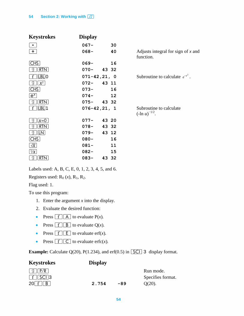
54 Section 2: Working with f
54
Keystrokes Display
- 067- 30
+ 068- 40 Adjusts integral for sign of x and
function.
” 069- 16
|n 070- 43 32
´b0 071-42,21, 0 Subroutine to calculate 2te .
|x 072- 43 11
” 073- 16
' 074- 12
|n 075- 43 32
´b1 076-42,21, 1 Subroutine to calculate
(-ln u)−1/2
.
|~ 077- 43 20
|n 078- 43 32
|N 079- 43 12
” 080- 16
¤ 081- 11
⁄ 082- 15
|n 083- 43 32
Labels used: A, B, C, E, 0, 1, 2, 3, 4, 5, and 6.
Registers used: R0 (x), R1, R2.
Flag used: 1.
To use this program:
1. Enter the argument x into the display.
2. Evaluate the desired function:
Press ´A to evaluate P(x).
Press ´B to evaluate Q(x).
Press ´E to evaluate erf(x).
Press ´C to evaluate erfc(x).
Example: Calculate Q(20), P(1.234), and erf(0.5) in i 3 display format.
Keystrokes Display
|¥ Run mode.
´i3 Specifies format.
20´B 2.754 -89 Q(20).
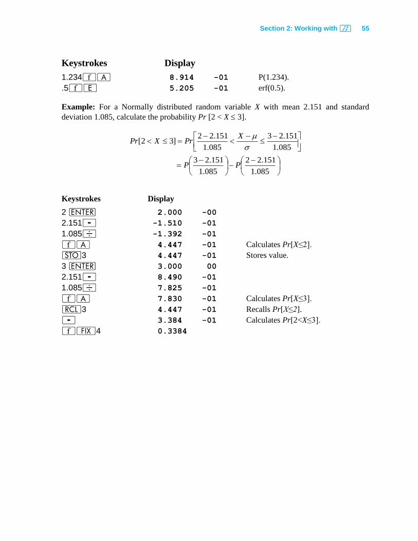
Section 2: Working with f 55
Keystrokes Display
1.234´A 8.914 -01 P(1.234).
.5´E 5.205 -01 erf(0.5).
Example: For a Normally distributed random variable X with mean 2.151 and standard
deviation 1.085, calculate the probability Pr [2 < X 3].
085.1
151.22
085.1
151.23
085.1
151.23
085.1
151.22]32[
PP
XPrXPr
Keystrokes Display
2 v 2.000 -00
2.151- -1.510 -01
1.085÷ -1.392 -01
´A 4.447 -01 Calculates Pr[X≤2].
O3 4.447 -01 Stores value.
3 v 3.000 00
2.151- 8.490 -01
1.085÷ 7.825 -01
´A 7.830 -01 Calculates Pr[X≤3].
l3 4.447 -01 Recalls Pr[X≤2].
- 3.384 -01 Calculates Pr[2<X≤3].
´•4 0.3384
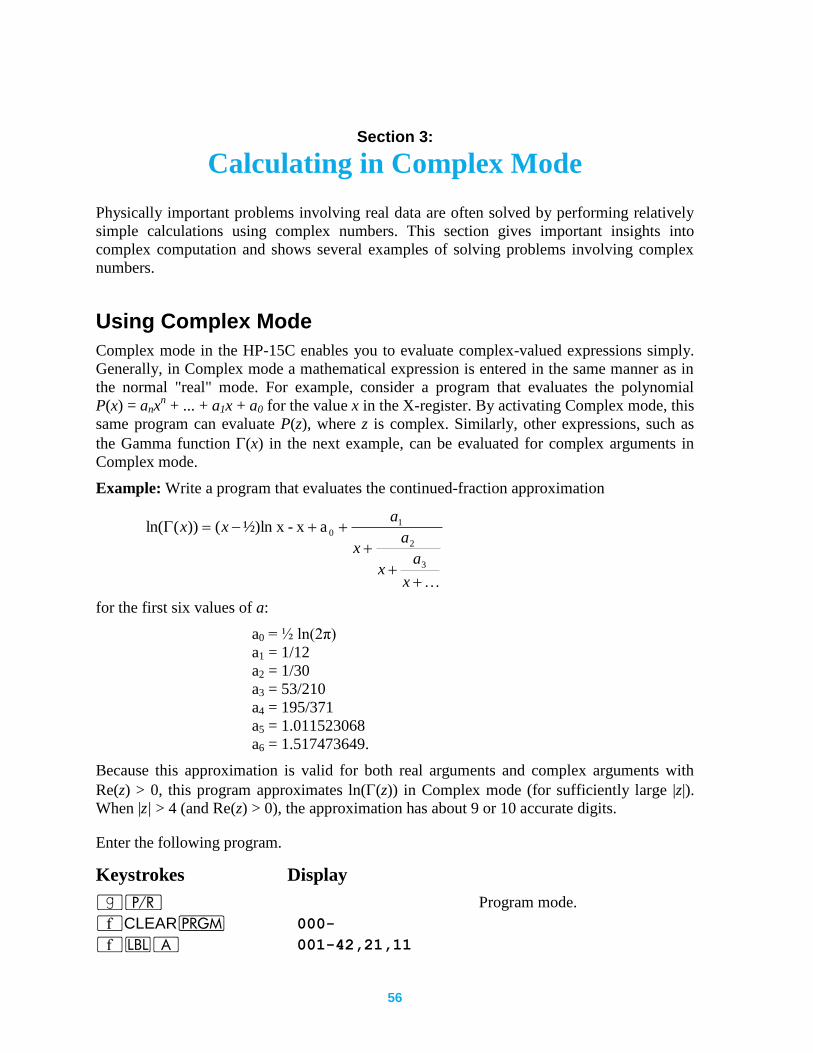
56
Section 3:
Calculating in Complex Mode
Physically important problems involving real data are often solved by performing relatively
simple calculations using complex numbers. This section gives important insights into
complex computation and shows several examples of solving problems involving complex
numbers.
Using Complex Mode
Complex mode in the HP-15C enables you to evaluate complex-valued expressions simply.
Generally, in Complex mode a mathematical expression is entered in the same manner as in
the normal "real" mode. For example, consider a program that evaluates the polynomial
P(x) = anxn + ... + a1x + a0 for the value x in the X-register. By activating Complex mode, this
same program can evaluate P(z), where z is complex. Similarly, other expressions, such as
the Gamma function (x) in the next example, can be evaluated for complex arguments in
Complex mode.
Example: Write a program that evaluates the continued-fraction approximation
x
ax
ax
axx
3
2
10a x-½)ln x())(ln(
for the first six values of a:
a0 = ½ ln(2π)
a1 = 1/12
a2 = 1/30
a3 = 53/210
a4 = 195/371
a5 = 1.011523068
a6 = 1.517473649.
Because this approximation is valid for both real arguments and complex arguments with
Re(z) > 0, this program approximates ln((z)) in Complex mode (for sufficiently large |z|).
When |z| > 4 (and Re(z) > 0), the approximation has about 9 or 10 accurate digits.
Enter the following program.
Keystrokes Display
|¥ Program mode.
´CLEARM 000-
´bA 001-42,21,11
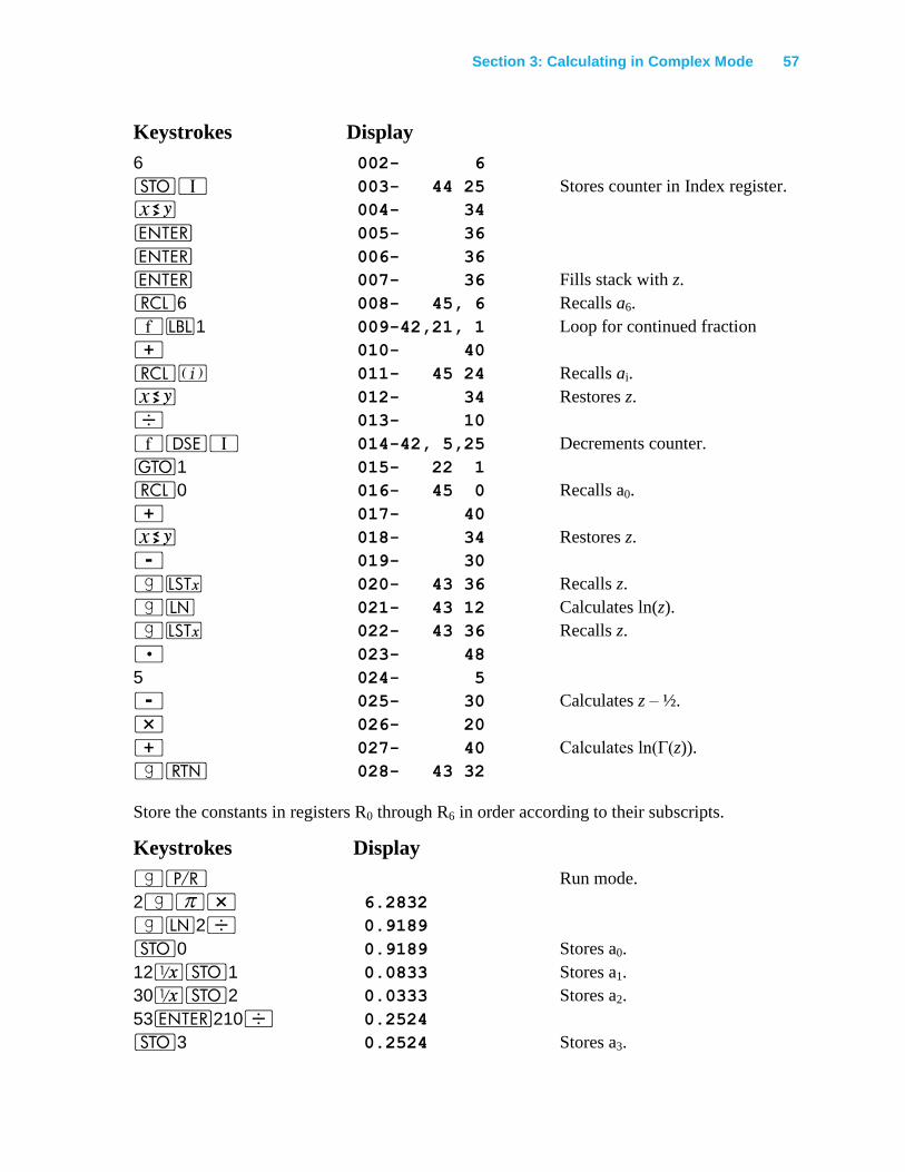
Section 3: Calculating in Complex Mode 57
Keystrokes Display
6 002- 6
OV 003- 44 25 Stores counter in Index register.
® 004- 34
v 005- 36
v 006- 36
v 007- 36 Fills stack with z.
l6 008- 45, 6 Recalls a6.
´b1 009-42,21, 1 Loop for continued fraction
+ 010- 40
l% 011- 45 24 Recalls ai.
® 012- 34 Restores z.
÷ 013- 10
´eV 014-42, 5,25 Decrements counter.
t1 015- 22 1
l0 016- 45 0 Recalls a0.
+ 017- 40
® 018- 34 Restores z.
- 019- 30
|K 020- 43 36 Recalls z.
|N 021- 43 12 Calculates ln(z).
|K 022- 43 36 Recalls z.
. 023- 48
5 024- 5
- 025- 30 Calculates z – ½.
* 026- 20
+ 027- 40 Calculates ln(Γ(z)).
|n 028- 43 32
Store the constants in registers R0 through R6 in order according to their subscripts.
Keystrokes Display
|¥ Run mode.
2|$* 6.2832
|N2÷ 0.9189
O0 0.9189 Stores a0.
12⁄O1 0.0833 Stores a1.
30⁄O2 0.0333 Stores a2.
53v210÷ 0.2524
O3 0.2524 Stores a3.
58 Section 3: Calculating in Complex Mode
58
Keystrokes Display
195v371÷ 0.5256
O4 0.5256 Stores a4.
1.011523068O5 1.0115 Stores a5.
1.517473649 O6 1.5175 Stores a6.
Use this program to calculate ln((4.2)), then compare it with ln(3.2!) calculated with the
! function. Also calculate ln((1 + 5i)).
Keystrokes Display
4.2´A 2.0486 Calculates ln((4.2)).
´•9 2.048555637 Displays 10 digits.
3.2´! 7.756689536 Calculates (3.2)! = (3.2+1).
|N 2.048555637 Calculates ln(3.2!).
1v 1.000000000 Enters real part of 1 + 5i.
5´V 1.000000000 Forms complex number
1 + 5i.
´A -6.130324145 Real part of ln((1 + 5i)).
´} 3.815898575 Imaginary part of
ln((1 + 5i)).
´•4 3.8159
The complex result is calculated with no more effort than that needed to enter the imaginary
part of the argument z. (The result ln((1 + 5i)) has 10 correct digits in each component.)
Trigonometric Modes
Although the trigonometric mode annunciator remains lit in Complex mode, complex
functions are always computed using radian measure. The annunciator indicates the mode
(Degrees, Radians, or Grads) for only the two complex conversions: : and ;.
If you want to evaluate rei
where is in degrees, ' can't be used directly because must
be in radians. If you attempt to convert from degrees to radians, there is a slight loss of
accuracy, especially at values like 180° for which the radian measure can't be represented
exactly with 10 digits.
However, in Complex mode the ; function computes rei
accurately for in any measure
(indicated by the annunciator). Simply enter r and into the complex X-registers in the form
r + i, then execute ; to calculate the complex value
rei
= r cos + ir sin .
(The program listed under Calculating the n th Roots of a Complex Number at the end of this
section uses this function.)
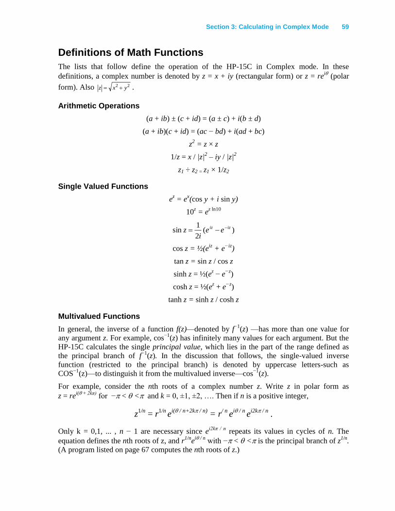
Section 3: Calculating in Complex Mode 59
Definitions of Math Functions
The lists that follow define the operation of the HP-15C in Complex mode. In these
definitions, a complex number is denoted by z = x + iy (rectangular form) or z = rei
(polar
form). Also 22 yxz .
Arithmetic Operations
(a + ib) ± (c + id) = (a ± c) + i(b ± d)
(a + ib)(c + id) = (ac − bd) + i(ad + bc)
z2 = z × z
1/z = x / |z|2 – iy / |z|
2
z1 ÷ z2 = z1 × 1/z2
Single Valued Functions
ez = e
x(cos y + i sin y)
10z = e
z ln10
)(2
1sin iziz ee
iz
cos z = ½(eiz + e
−iz)
tan z = sin z / cos z
sinh z = ½(ez − e
−z)
cosh z = ½(ez + e
−z)
tanh z = sinh z / cosh z
Multivalued Functions
In general, the inverse of a function f(z)—denoted by f−1
(z) —has more than one value for
any argument z. For example, cos−1
(z) has infinitely many values for each argument. But the
HP-15C calculates the single principal value, which lies in the part of the range defined as
the principal branch of f−1
(z). In the discussion that follows, the single-valued inverse
function (restricted to the principal branch) is denoted by uppercase letters-such as
COS−1
(z)—to distinguish it from the multivalued inverse—cos−1
(z).
For example, consider the nth roots of a complex number z. Write z in polar form as
z = rei( + 2kπ)
for − < < and k = 0, ±1, ±2, …. Then if n is a positive integer,
z1/n
= r1/n
ei( / n+2k / n)
= r/ n
ei / n
ei2k / n
.
Only k = 0,1, ... , n − 1 are necessary since ei2kπ / n
repeats its values in cycles of n. The
equation defines the nth roots of z, and r1/n
ei / n
with − < < is the principal branch of z1/n
.
(A program listed on page 67 computes the nth roots of z.)
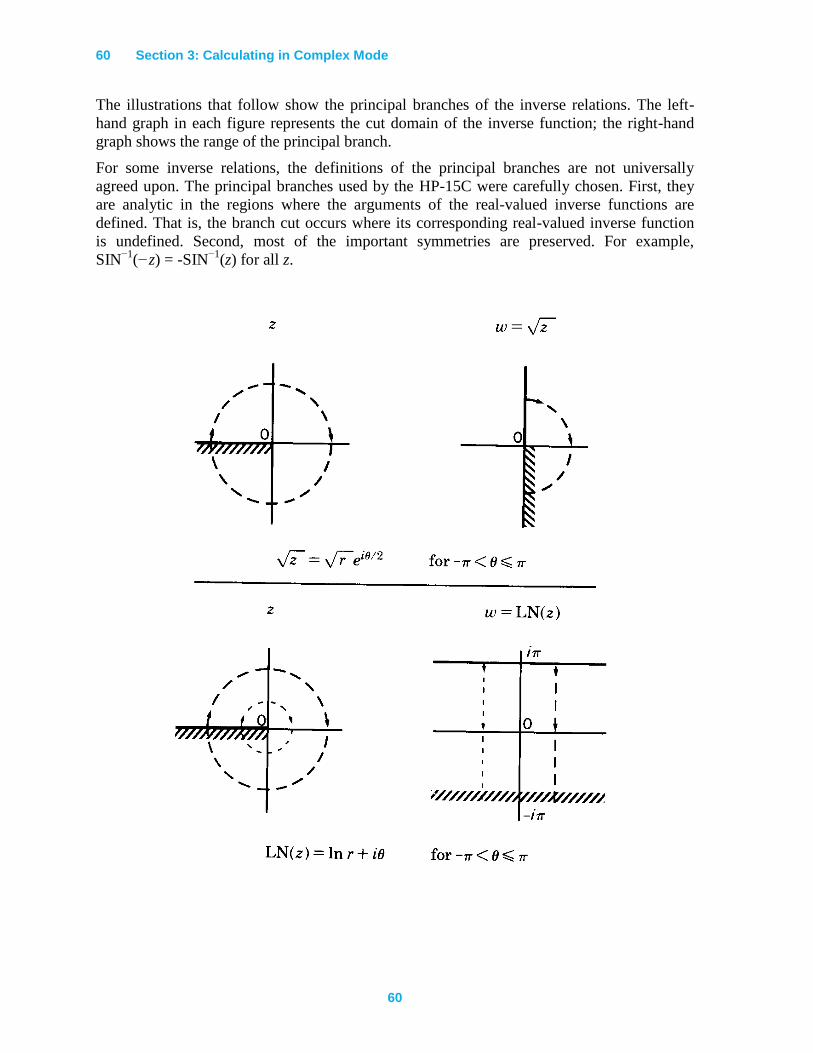
60 Section 3: Calculating in Complex Mode
60
The illustrations that follow show the principal branches of the inverse relations. The left-
hand graph in each figure represents the cut domain of the inverse function; the right-hand
graph shows the range of the principal branch.
For some inverse relations, the definitions of the principal branches are not universally
agreed upon. The principal branches used by the HP-15C were carefully chosen. First, they
are analytic in the regions where the arguments of the real-valued inverse functions are
defined. That is, the branch cut occurs where its corresponding real-valued inverse function
is undefined. Second, most of the important symmetries are preserved. For example,
SIN−1
(−z) = -SIN−1
(z) for all z.
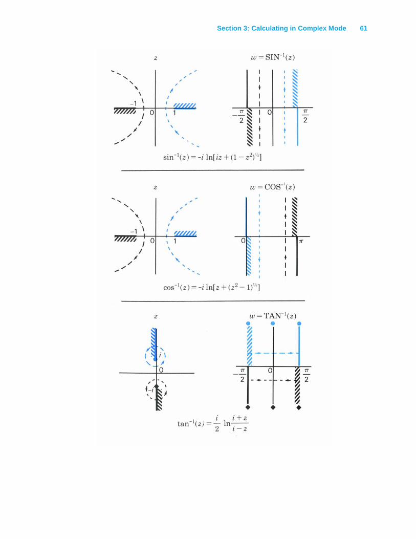
Section 3: Calculating in Complex Mode 61
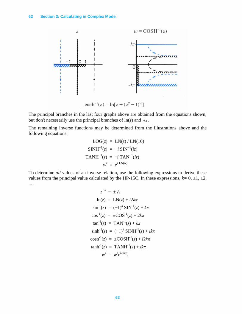
62 Section 3: Calculating in Complex Mode
62
The principal branches in the last four graphs above are obtained from the equations shown,
but don't necessarily use the principal branches of ln(z) and z .
The remaining inverse functions may be determined from the illustrations above and the
following equations:
LOG(z) = LN(z) / LN(10)
SINH−1
(z) = −i SIN−1
(iz)
TANH−1
(z) = −i TAN−1
(iz)
wz = e
z LN(w).
To determine all values of an inverse relation, use the following expressions to derive these
values from the principal value calculated by the HP-15C. In these expressions, k= 0, ±1, ±2,
... .
z ½ = ± z
ln(z) = LN(z) + i2kπ
sin-1
(z) = (−1)k SIN
-1(z) + kπ
cos-1
(z) = ±COS-1
(z) + 2kπ
tan-1
(z) = TAN-1
(z) + kπ
sinh-1
(z) = (−1)k SINH
-1(z) + ikπ
cosh-1
(z) = ±COSH-1
(z) + i2kπ
tanh-1
(z) = TANH-1
(z) + ikπ
wz = w
ze
i2πkz.
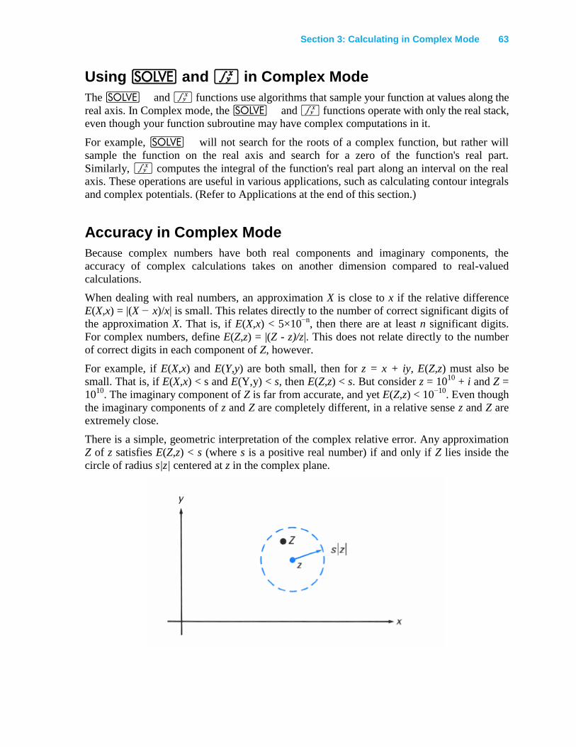
Section 3: Calculating in Complex Mode 63
Using _ and f in Complex Mode
The _ and f functions use algorithms that sample your function at values along the
real axis. In Complex mode, the _ and f functions operate with only the real stack,
even though your function subroutine may have complex computations in it.
For example, _ will not search for the roots of a complex function, but rather will
sample the function on the real axis and search for a zero of the function's real part.
Similarly, f computes the integral of the function's real part along an interval on the real
axis. These operations are useful in various applications, such as calculating contour integrals
and complex potentials. (Refer to Applications at the end of this section.)
Accuracy in Complex Mode
Because complex numbers have both real components and imaginary components, the
accuracy of complex calculations takes on another dimension compared to real-valued
calculations.
When dealing with real numbers, an approximation X is close to x if the relative difference
E(X,x) = |(X − x)/x| is small. This relates directly to the number of correct significant digits of
the approximation X. That is, if E(X,x) < 5×10−n
, then there are at least n significant digits.
For complex numbers, define E(Z,z) = |(Z - z)/z|. This does not relate directly to the number
of correct digits in each component of Z, however.
For example, if E(X,x) and E(Y,y) are both small, then for z = x + iy, E(Z,z) must also be
small. That is, if E(X,x) < s and E(Y,y) < s, then E(Z,z) < s. But consider z = 1010
+ i and Z =
1010
. The imaginary component of Z is far from accurate, and yet E(Z,z) < 10−10
. Even though
the imaginary components of z and Z are completely different, in a relative sense z and Z are
extremely close.
There is a simple, geometric interpretation of the complex relative error. Any approximation
Z of z satisfies E(Z,z) < s (where s is a positive real number) if and only if Z lies inside the
circle of radius s|z| centered at z in the complex plane.
64 Section 3: Calculating in Complex Mode
64
To require approximations with accurate components is to demand more than keeping
relative errors small. For example, consider this problem in which the calculations are done
with four significant digits. It illustrates the limitations imposed on a complex calculation by
finite accuracy.
z1 = Z1 = 37.1 + 37.3i
z2 = Z2 = 37.5 + 37.3i
and
Z1 × Z2
= (37.10 × 37.50 − 37.30 × 37.30) + i(37.10 × 37.30 + 37.30 × 37.50)
= (1391. − 1391.) + i(1384. + 1399.)
= 0 + i(2783.)
The true value z1z2 = −0.04 + 2782.58i. Even though Z1 and Z2 have no error, the real part of
their four-digit product has no correct significant decimals, although the relative error of the
complex product is less than 2 × 10⁻⁴
.
The example illustrates that complex multiplication doesn't propagate its errors component
wise. But even if complex multiplication produced accurate components, the rounding errors
of a chain computation could quickly produce inaccurate components. On the other hand, the
relative error, which corresponds to the precision of the calculation, grows only slowly.
For example, using four-digit accuracy as before
z1 = (1 + 1/300) + i
Z1 = 1.003 + i
z2 = Z2 = 1 + i
then
Z1 × Z2 = (1.003 + i) × (1 + i)
= 0.003 + 2.003i
= 3.000 × 10⁻³
+ 2.003i
The correct four-digit value is 3.333 × 10⁻³
+ 2.003i. In this example, Zl and Z2 are accurate
in each component and the arithmetic is exact. But the product is inaccurate-that is, the real
component has only one significant digit. One rounding error causes an inaccurate
component, although the complex relative error of the product remains small.
For the HP-15C the results of any complex operation are designed to be accurate in the sense
that the complex relative error E(Z,z) is kept small. Generally, E(Z,z) < 6 × 10⁻¹⁰
.
As shown earlier, this small relative error doesn't guarantee 10 accurate digits in each
component. Because the error is relative to the size |z|, and because this is not greatly
different from the size of the largest component of z, the smaller component can have fewer
accurate digits. There is a quick way for you to see which digits are generally accurate.
Express each component using the largest exponent. In this form, approximately the first 10
digits of each component are accurate. For example, if
Z = 1.234567890 × 10⁻¹⁰
+ i(2.222222222 × 10⁻³
),

Section 3: Calculating in Complex Mode 65
then think of Z as
0.0000001234567890 × 10⁻³
+ i(2.222222222 × 10⁻³
).
then the accurate digits are
0.000000123 × 10⁻³
+ i(2.222222222 × 10⁻³
).
Applications
The capability of the HP-15C to work with complex numbers enables you to solve problems
that extend beyond the realm of real-valued numbers. On the following pages are several
programs that illustrate the usefulness of complex calculations—and the HP-15C.
Storing and Recalling Complex Numbers Using a Matrix
This program uses the stack and matrix C to store and recall complex numbers. It has the
following characteristics:
If you specify an index greater than the matrix's dimensions, the calculator displays
Error 3 and the stack is ready for another try.
If the calculator isn't in Complex mode, the program activates Complex mode and the
imaginary part of the number is set to zero.
When you store a complex number, the index is lost, the stack drops, and the
T-register is duplicated in the Z-register.
The "Store" program uses the Á key, which is above the O key. The "Recall"
program uses the E key, which is above the l key.
Keystrokes Display
|¥ Program mode.
´ CLEARM 000-
´bÁ 001-42,21,14 “Store” program.
´>1 002-42,16, 1 Sets R0 = R1 = 1.
O0 003- 44 0 R0 = k.
) 004- 33
0 005- 0 Enters 0 in real (and imaginary)
X-registers.
+ 006- 40 Drops stack and has a + ib in
X-register.
´UOC ´U
007u 44 13 Stores a and increments indices
(User mode).
´} 008- 42 30
OC 009- 44 13 Stores b (no User mode here).
´} 010- 42 30 Restores a + ib in X-registers.
66 Section 3: Calculating in Complex Mode
66
Keystrokes Display
|n 011- 43 32
´bE 012-42,21,15 “Recall” program.
O0 013- 44 0 R0 = k.
|` 014- 43 35 Disables stack.
2 015- 2
O1 016- 44 1 Sets R1 = 2.
) 017- 33
0 018- 0
+ 019- 40 Sets stack for another try if
Error 3 occurs next.
lC 020- 45 13 Recalls b (imaginary part).
´} 021- 42 30
´s1 022-42, 5, 1 Decrements R1 = 1.
|` 023- 43 35 Disables stack and clears real
X-register.
lC 024- 45 13 Recalls a (real part).
|n 025- 43 32
Example: Store 2 + 3i and 7 + 4i in elements 1 and 2 using the previous program. Then
recall and add them. Dimension matrix C to 5 x 2 so that it can store up to 5 complex
numbers.
After entering the preceding program:
Keystrokes Display
|¥ Run mode.
5v2 2 Specifies 5 rows and 2
columns.
´mC 2.0000 Dimensions matrix C.
2v3´V 2.0000 Enters 2 + 3i.
1´Á 2.0000 Stores number in C using
index 1.
7v4´V 7.0000 Enters 7 + 4i.
2´Á 7.0000 Stores number in C using
index 2.
1´E 2.0000 Recalls first number.
2´E 7.0000 Recalls second number.
+ 9.0000 Real part of sum.
´} 7.0000 Imaginary part of sum.
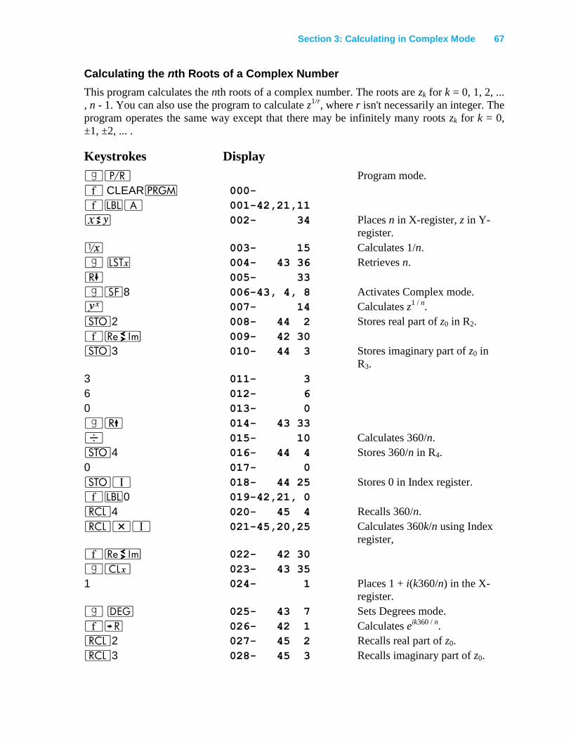
Section 3: Calculating in Complex Mode 67
Calculating the nth Roots of a Complex Number
This program calculates the nth roots of a complex number. The roots are zk for k = 0, 1, 2, ...
, n - 1. You can also use the program to calculate z1/r
, where r isn't necessarily an integer. The
program operates the same way except that there may be infinitely many roots zk for k = 0,
±1, ±2, ... .
Keystrokes Display
|¥ Program mode.
´ CLEARM 000-
´bA 001-42,21,11
® 002- 34 Places n in X-register, z in Y-
register.
⁄ 003- 15 Calculates 1/n.
| K 004- 43 36 Retrieves n.
) 005- 33
|F8 006-43, 4, 8 Activates Complex mode.
Y 007- 14 Calculates z1 / n
.
O2 008- 44 2 Stores real part of z0 in R2.
´} 009- 42 30
O3 010- 44 3 Stores imaginary part of z0 in
R3.
3 011- 3
6 012- 6
0 013- 0
|( 014- 43 33
÷ 015- 10 Calculates 360/n.
O4 016- 44 4 Stores 360/n in R4.
0 017- 0
OV 018- 44 25 Stores 0 in Index register.
´b0 019-42,21, 0
l4 020- 45 4 Recalls 360/n.
l*V 021-45,20,25 Calculates 360k/n using Index
register,
´} 022- 42 30
|` 023- 43 35
1 024- 1 Places 1 + i(k360/n) in the X-
register.
| D 025- 43 7 Sets Degrees mode.
´; 026- 42 1 Calculates eik360 / n
.
l2 027- 45 2 Recalls real part of z0.
l3 028- 45 3 Recalls imaginary part of z0.
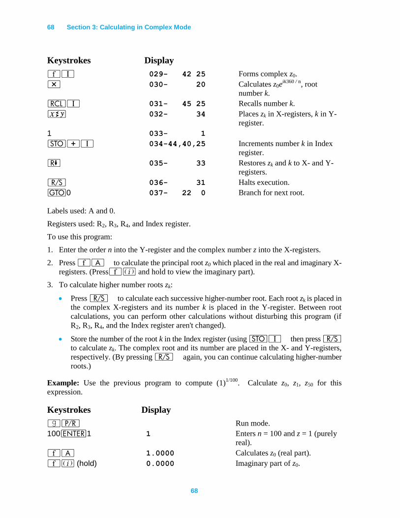
68 Section 3: Calculating in Complex Mode
68
Keystrokes Display
´V 029- 42 25 Forms complex z0.
* 030- 20 Calculates z0eik360 / n
, root
number k.
lV 031- 45 25 Recalls number k.
® 032- 34 Places zk in X-registers, k in Y-
register.
1 033- 1
O+V 034-44,40,25 Increments number k in Index
register.
) 035- 33 Restores zk and k to X- and Y-
registers.
¦ 036- 31 Halts execution.
t0 037- 22 0 Branch for next root.
Labels used: A and 0.
Registers used: R2, R3, R4, and Index register.
To use this program:
1. Enter the order n into the Y-register and the complex number z into the X-registers.
2. Press ´A to calculate the principal root z0 which placed in the real and imaginary X-
registers. (Press´% and hold to view the imaginary part).
3. To calculate higher number roots zk:
Press ¦ to calculate each successive higher-number root. Each root zk is placed in
the complex X-registers and its number k is placed in the Y-register. Between root
calculations, you can perform other calculations without disturbing this program (if
R2, R3, R4, and the Index register aren't changed).
Store the number of the root k in the Index register (using OV then press ¦ to calculate zk. The complex root and its number are placed in the X- and Y-registers,
respectively. (By pressing ¦ again, you can continue calculating higher-number
roots.)
Example: Use the previous program to compute (1)1/100
. Calculate z0, z1, z50 for this
expression.
Keystrokes Display
|¥ Run mode.
100v1 1 Enters n = 100 and z = 1 (purely
real).
´A 1.0000 Calculates z0 (real part).
´% (hold) 0.0000 Imaginary part of z0.
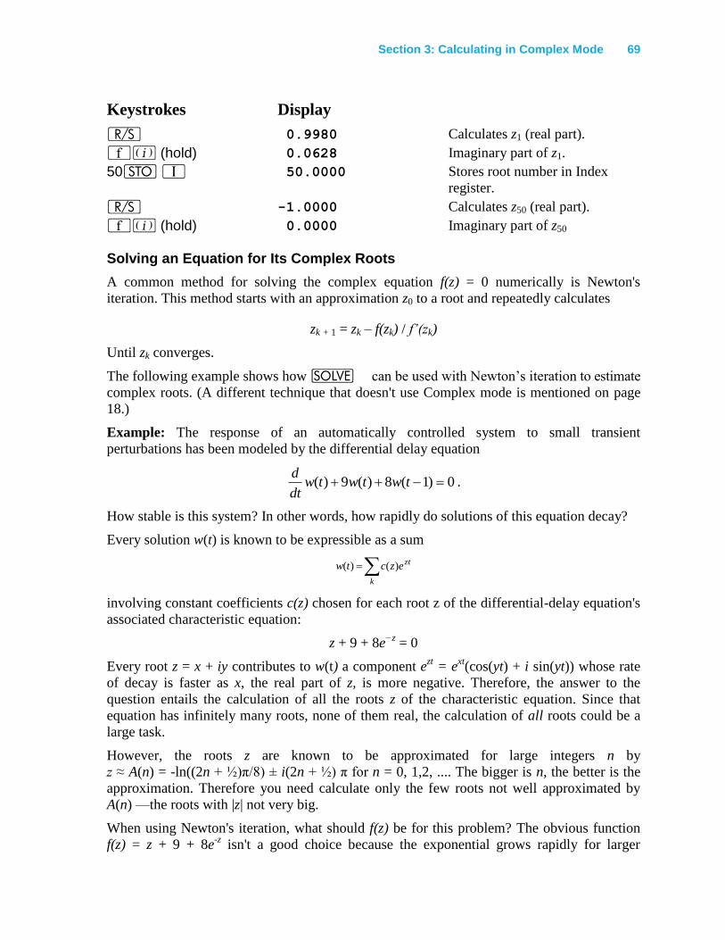
Section 3: Calculating in Complex Mode 69
Keystrokes Display
¦ 0.9980 Calculates z1 (real part).
´% (hold) 0.0628 Imaginary part of z1.
50O V 50.0000 Stores root number in Index
register.
¦ -1.0000 Calculates z50 (real part).
´% (hold) 0.0000 Imaginary part of z50
Solving an Equation for Its Complex Roots
A common method for solving the complex equation f(z) = 0 numerically is Newton's
iteration. This method starts with an approximation z0 to a root and repeatedly calculates
zk + 1 = zk – f(zk) / f’(zk)
Until zk converges.
The following example shows how _ can be used with Newton’s iteration to estimate
complex roots. (A different technique that doesn't use Complex mode is mentioned on page
18.)
Example: The response of an automatically controlled system to small transient
perturbations has been modeled by the differential delay equation
0)1(8)(9)( twtwtwdt
d.
How stable is this system? In other words, how rapidly do solutions of this equation decay?
Every solution w(t) is known to be expressible as a sum
k
ztezctw )()(
involving constant coefficients c(z) chosen for each root z of the differential-delay equation's
associated characteristic equation:
z + 9 + 8e−z
= 0
Every root z = x + iy contributes to w(t) a component ezt = e
xt(cos(yt) + i sin(yt)) whose rate
of decay is faster as x, the real part of z, is more negative. Therefore, the answer to the
question entails the calculation of all the roots z of the characteristic equation. Since that
equation has infinitely many roots, none of them real, the calculation of all roots could be a
large task.
However, the roots z are known to be approximated for large integers n by
z ≈ A(n) = -ln((2n + ½)π/8) ± i(2n + ½) π for n = 0, 1,2, .... The bigger is n, the better is the
approximation. Therefore you need calculate only the few roots not well approximated by
A(n) —the roots with |z| not very big.
When using Newton's iteration, what should f(z) be for this problem? The obvious function
f(z) = z + 9 + 8e-z isn't a good choice because the exponential grows rapidly for larger
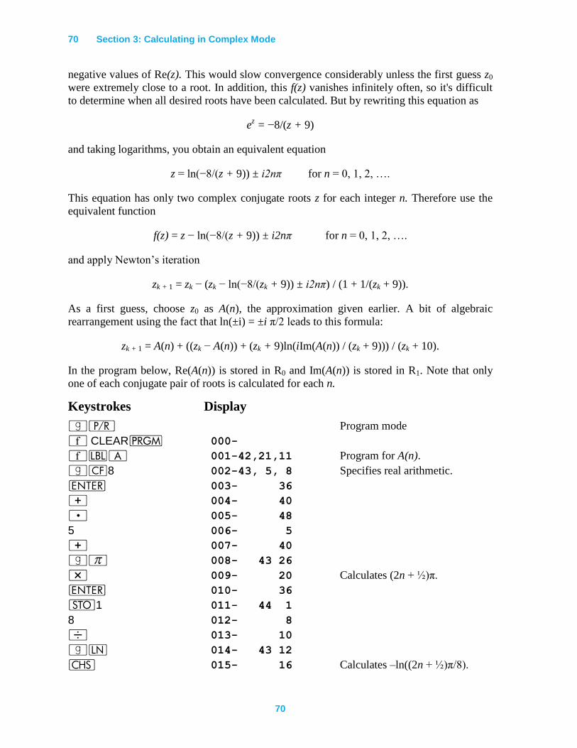
70 Section 3: Calculating in Complex Mode
70
negative values of Re(z). This would slow convergence considerably unless the first guess z0
were extremely close to a root. In addition, this f(z) vanishes infinitely often, so it's difficult
to determine when all desired roots have been calculated. But by rewriting this equation as
ez = −8/(z + 9)
and taking logarithms, you obtain an equivalent equation
z = ln(−8/(z + 9)) ± i2nπ for n = 0, 1, 2, ….
This equation has only two complex conjugate roots z for each integer n. Therefore use the
equivalent function
f(z) = z − ln(−8/(z + 9)) ± i2nπ for n = 0, 1, 2, ….
and apply Newton’s iteration
zk + 1 = zk − (zk − ln(−8/(zk + 9)) ± i2nπ) / (1 + 1/(zk + 9)).
As a first guess, choose z0 as A(n), the approximation given earlier. A bit of algebraic
rearrangement using the fact that ln(±i) = ±i π/2 leads to this formula:
zk + 1 = A(n) + ((zk − A(n)) + (zk + 9)ln(iIm(A(n)) / (zk + 9))) / (zk + 10).
In the program below, Re(A(n)) is stored in R0 and Im(A(n)) is stored in R1. Note that only
one of each conjugate pair of roots is calculated for each n.
Keystrokes Display
|¥ Program mode
´ CLEARM 000-
´bA 001-42,21,11 Program for A(n).
|"8 002-43, 5, 8 Specifies real arithmetic.
v 003- 36
+ 004- 40
. 005- 48
5 006- 5
+ 007- 40
|$ 008- 43 26
* 009- 20 Calculates (2n + ½)π.
v 010- 36
O1 011- 44 1
8 012- 8
÷ 013- 10
|N 014- 43 12
” 015- 16 Calculates –ln((2n + ½)π/8).
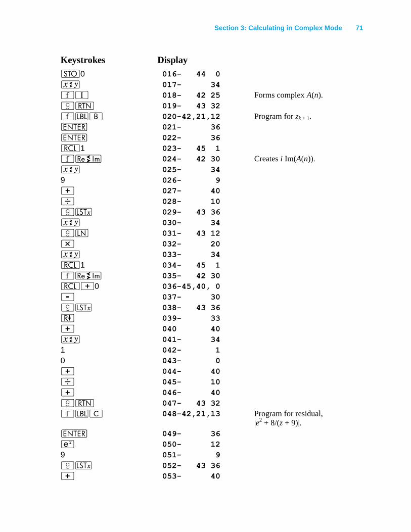
Section 3: Calculating in Complex Mode 71
Keystrokes Display
O0 016- 44 0
® 017- 34
´V 018- 42 25 Forms complex A(n).
|n 019- 43 32
´bB 020-42,21,12 Program for zk + 1.
v 021- 36
v 022- 36
l1 023- 45 1
´} 024- 42 30 Creates i Im(A(n)).
® 025- 34
9 026- 9
+ 027- 40
÷ 028- 10
|K 029- 43 36
® 030- 34
|N 031- 43 12
* 032- 20
® 033- 34
l1 034- 45 1
´} 035- 42 30
l+0 036-45,40, 0
- 037- 30
|K 038- 43 36
) 039- 33
+ 040 40
® 041- 34
1 042- 1
0 043- 0
+ 044- 40
÷ 045- 10
+ 046- 40
|n 047- 43 32
´bC 048-42,21,13 Program for residual,
|e2 + 8/(z + 9)|.
v 049- 36
' 050- 12
9 051- 9
|K 052- 43 36
+ 053- 40
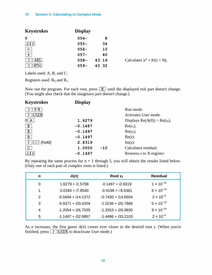
72 Section 3: Calculating in Complex Mode
72
Keystrokes Display
8 054- 8
® 055- 34
÷ 056- 10
+ 057- 40
|a 058- 43 16 Calculates |ez + 8/(z + 9)|.
|n 059- 43 32
Labels used: A, B, and C.
Registers used: R0 and R1.
Now run the program. For each root, press B until the displayed real part doesn't change.
(You might also check that the imaginary part doesn't change.)
Keystrokes Display
|¥ Run mode.
´U Activates User mode.
0A 1.6279 Displays Re(A(0)) = Re(z0).
B -0.1487 Re(z1).
B -0.1497 Re(z2).
B -0.1497 Re(z).
´% (hold) 2.8319 Im(z).
C 1.0000 -10 Calculates residual.
® -0.1497 Restores z to X-register.
By repeating the same process for n = 1 through 5, you will obtain the results listed below.
(Only one of each pair of complex roots is listed.)
n A(n) Root zk Residual
0 1.6279 + i1.5708 -0.1497 + i2.8319 1 × 10⁻¹⁰
1 0.0184 + i7.8540 -0.4198 + i 8.6361 6 × 10⁻¹⁰
2 -0.5694 + i14.1372 -0.7430 + i14.6504 2 × 10⁻⁹
3 -0.9371 + i20.4204 -1.0236 + i20.7868 5 × 10⁻¹⁰
4 -1.2054 + i26.7035 -1.2553 + i26.9830 9 × 10⁻¹⁰
5 -1.1467 + i32.9867 -1.4486 + i33.2103 2 × 10⁻⁹
As n increases, the first guess A(n) comes ever closer to the desired root z. (When you're
finished, press ´U to deactivate User mode.)
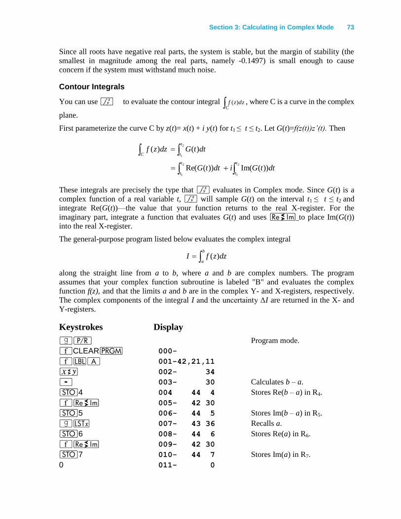
Section 3: Calculating in Complex Mode 73
Since all roots have negative real parts, the system is stable, but the margin of stability (the
smallest in magnitude among the real parts, namely -0.1497) is small enough to cause
concern if the system must withstand much noise.
Contour Integrals
You can use f to evaluate the contour integral C dzzf )( , where C is a curve in the complex
plane.
First parameterize the curve C by z(t)= x(t) + i y(t) for t1 ≤ t ≤ t2. Let G(t)=f(z(t))z’(t). Then
2
1
2
1
2
1
))(Im())(Re(
)()(
t
t
t
t
C
t
t
dttGidttG
dttGdzzf
These integrals are precisely the type that f evaluates in Complex mode. Since G(t) is a
complex function of a real variable t, f will sample G(t) on the interval t1 ≤ t ≤ t2 and
integrate Re(G(t))—the value that your function returns to the real X-register. For the
imaginary part, integrate a function that evaluates G(t) and uses } to place Im(G(t))
into the real X-register.
The general-purpose program listed below evaluates the complex integral
b
adzzfI )(
along the straight line from a to b, where a and b are complex numbers. The program
assumes that your complex function subroutine is labeled "B" and evaluates the complex
function f(z), and that the limits a and b are in the complex Y- and X-registers, respectively.
The complex components of the integral I and the uncertainty ΔI are returned in the X- and
Y-registers.
Keystrokes Display
|¥ Program mode.
´CLEARM 000-
´bA 001-42,21,11
® 002- 34
- 003- 30 Calculates b – a.
O4 004 44 4 Stores Re(b – a) in R4.
´} 005- 42 30
O5 006- 44 5 Stores Im(b – a) in R5.
|K 007- 43 36 Recalls a.
O6 008- 44 6 Stores Re(a) in R6.
´} 009- 42 30
O7 010- 44 7 Stores Im(a) in R7.
0 011- 0
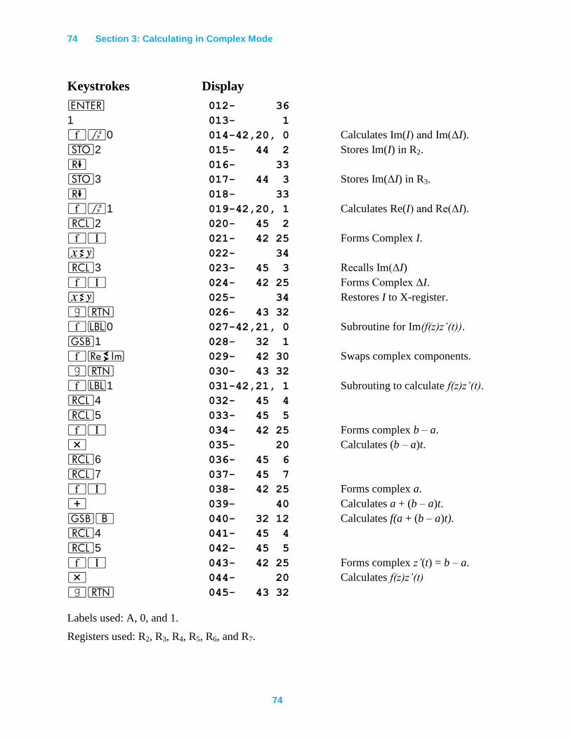
74 Section 3: Calculating in Complex Mode
74
Keystrokes Display
v 012- 36
1 013- 1
´f0 014-42,20, 0 Calculates Im(I) and Im(ΔI).
O2 015- 44 2 Stores Im(I) in R2.
) 016- 33
O3 017- 44 3 Stores Im(ΔI) in R3.
) 018- 33
´f1 019-42,20, 1 Calculates Re(I) and Re(ΔI).
l2 020- 45 2
´V 021- 42 25 Forms Complex I.
® 022- 34
l3 023- 45 3 Recalls Im(ΔI)
´V 024- 42 25 Forms Complex ΔI.
® 025- 34 Restores I to X-register.
|n 026- 43 32
´b0 027-42,21, 0 Subroutine for Im(f(z)z’(t)).
G1 028- 32 1
´} 029- 42 30 Swaps complex components.
|n 030- 43 32
´b1 031-42,21, 1 Subrouting to calculate f(z)z’(t).
l4 032- 45 4
l5 033- 45 5
´V 034- 42 25 Forms complex b – a.
* 035- 20 Calculates (b – a)t.
l6 036- 45 6
l7 037- 45 7
´V 038- 42 25 Forms complex a.
+ 039- 40 Calculates a + (b – a)t.
GB 040- 32 12 Calculates f(a + (b – a)t).
l4 041- 45 4
l5 042- 45 5
´V 043- 42 25 Forms complex z’(t) = b – a.
* 044- 20 Calculates f(z)z’(t)
|n 045- 43 32
Labels used: A, 0, and 1.
Registers used: R2, R3, R4, R5, R6, and R7.
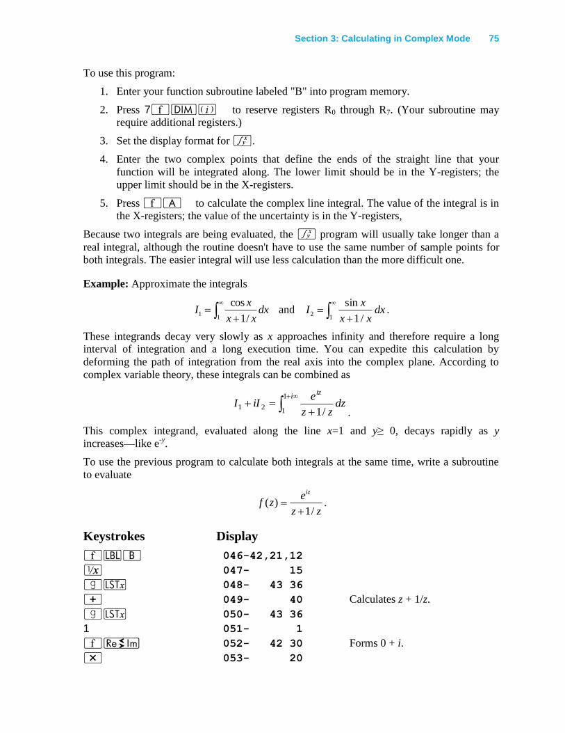
Section 3: Calculating in Complex Mode 75
To use this program:
1. Enter your function subroutine labeled "B" into program memory.
2. Press 7´m% to reserve registers R0 through R7. (Your subroutine may
require additional registers.)
3. Set the display format for f.
4. Enter the two complex points that define the ends of the straight line that your
function will be integrated along. The lower limit should be in the Y-registers; the
upper limit should be in the X-registers.
5. Press ´A to calculate the complex line integral. The value of the integral is in
the X-registers; the value of the uncertainty is in the Y-registers,
Because two integrals are being evaluated, the f program will usually take longer than a
real integral, although the routine doesn't have to use the same number of sample points for
both integrals. The easier integral will use less calculation than the more difficult one.
Example: Approximate the integrals
11
/1
cosdx
xx
xI and
12
/1
sindx
xx
xI .
These integrands decay very slowly as x approaches infinity and therefore require a long
interval of integration and a long execution time. You can expedite this calculation by
deforming the path of integration from the real axis into the complex plane. According to
complex variable theory, these integrals can be combined as
iiz
dzzz
eiII
1
121
/1 .
This complex integrand, evaluated along the line x=1 and y≥ 0, decays rapidly as y
increases—like e-y
.
To use the previous program to calculate both integrals at the same time, write a subroutine
to evaluate
zz
ezf
iz
/1)(
.
Keystrokes Display
´bB 046-42,21,12
⁄ 047- 15
|K 048- 43 36
+ 049- 40 Calculates z + 1/z.
|K 050- 43 36
1 051- 1
´} 052- 42 30 Forms 0 + i.
* 053- 20
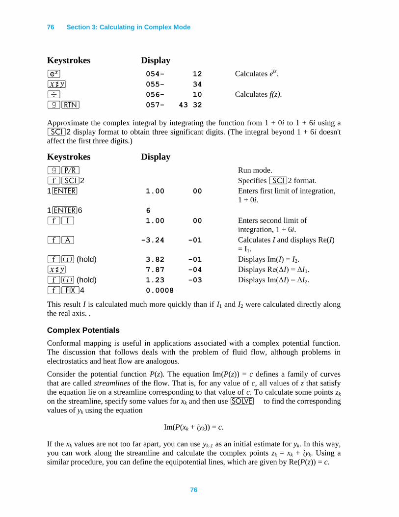
76 Section 3: Calculating in Complex Mode
76
Keystrokes Display
' 054- 12 Calculates eiz.
® 055- 34
÷ 056- 10 Calculates f(z).
|n 057- 43 32
Approximate the complex integral by integrating the function from 1 + 0i to 1 + 6i using a
i2 display format to obtain three significant digits. (The integral beyond 1 + 6i doesn't
affect the first three digits.)
Keystrokes Display
|¥ Run mode.
´i2 Specifies i2 format.
1v 1.00 00 Enters first limit of integration,
1 + 0i.
1v6 6
´V 1.00 00 Enters second limit of
integration, 1 + 6i.
´A -3.24 -01 Calculates I and displays Re(I)
= I1.
´% (hold) 3.82 -01 Displays Im(I) = I2.
® 7.87 -04 Displays Re(ΔI) = ΔI1.
´% (hold) 1.23 -03 Displays Im(ΔI) = ΔI2.
´•4 0.0008
This result I is calculated much more quickly than if I1 and I2 were calculated directly along
the real axis. .
Complex Potentials
Conformal mapping is useful in applications associated with a complex potential function.
The discussion that follows deals with the problem of fluid flow, although problems in
electrostatics and heat flow are analogous.
Consider the potential function P(z). The equation Im(P(z)) = c defines a family of curves
that are called streamlines of the flow. That is, for any value of c, all values of z that satisfy
the equation lie on a streamline corresponding to that value of c. To calculate some points zk
on the streamline, specify some values for xk and then use _ to find the corresponding
values of yk using the equation
Im(P(xk + iyk)) = c.
If the xk values are not too far apart, you can use yk-1 as an initial estimate for yk. In this way,
you can work along the streamline and calculate the complex points zk = xk + iyk. Using a
similar procedure, you can define the equipotential lines, which are given by Re(P(z)) = c.
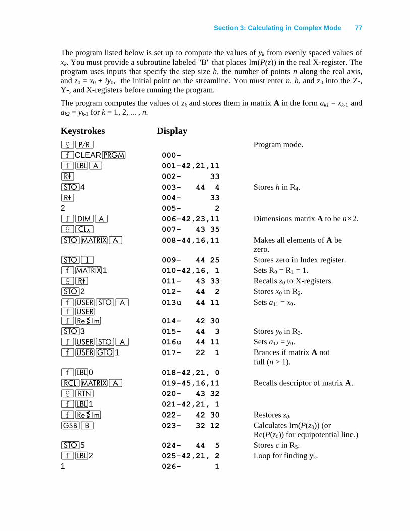
Section 3: Calculating in Complex Mode 77
The program listed below is set up to compute the values of yk from evenly spaced values of
xk. You must provide a subroutine labeled "B" that places Im(P(z)) in the real X-register. The
program uses inputs that specify the step size h, the number of points n along the real axis,
and z0 = x0 + iy0, the initial point on the streamline. You must enter n, h, and z0 into the Z-,
Y-, and X-registers before running the program.
The program computes the values of zk and stores them in matrix A in the form ak1 = xk-1 and
ak2 = yk-1 for k = 1, 2, ... , n.
Keystrokes Display
|¥ Program mode.
´CLEARM 000-
´bA 001-42,21,11
) 002- 33
O4 003- 44 4 Stores h in R4.
) 004- 33
2 005- 2
´mA 006-42,23,11 Dimensions matrix A to be n×2.
|` 007- 43 35
O>A 008-44,16,11 Makes all elements of A be
zero.
OV 009- 44 25 Stores zero in Index register.
´>1 010-42,16, 1 Sets R0 = R1 = 1.
|( 011- 43 33 Recalls z0 to X-registers.
O2 012- 44 2 Stores x0 in R2.
´UOA ´U
013u 44 11 Sets a11 = x0.
´} 014- 42 30
O3 015- 44 3 Stores y0 in R3.
´UOA 016u 44 11 Sets a12 = y0.
´Ut1 017- 22 1 Brances if matrix A not
full (n > 1).
´b0 018-42,21, 0
l>A 019-45,16,11 Recalls descriptor of matrix A.
|n 020- 43 32
´b1 021-42,21, 1
´} 022- 42 30 Restores z0.
GB 023- 32 12 Calculates Im(P(z0)) (or
Re(P(z0)) for equipotential line.)
O5 024- 44 5 Stores c in R5.
´b2 025-42,21, 2 Loop for finding yk.
1 026- 1
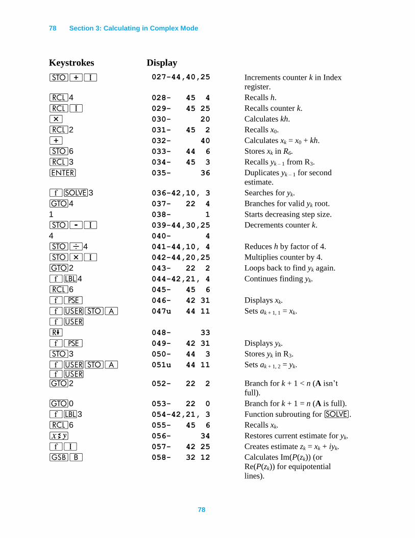
78 Section 3: Calculating in Complex Mode
78
Keystrokes Display
O+V 027-44,40,25 Increments counter k in Index
register.
l4 028- 45 4 Recalls h.
lV 029- 45 25 Recalls counter k.
* 030- 20 Calculates kh.
l2 031- 45 2 Recalls x0.
+ 032- 40 Calculates xk = x0 + kh.
O6 033- 44 6 Stores xk in R6.
l3 034- 45 3 Recalls yk – 1 from R3.
v 035- 36 Duplicates yk – 1 for second
estimate.
´_3 036-42,10, 3 Searches for yk.
t4 037- 22 4 Branches for valid yk root.
1 038- 1 Starts decreasing step size.
O-V 039-44,30,25 Decrements counter k.
4 040- 4
O÷4 041-44,10, 4 Reduces h by factor of 4.
O*V 042-44,20,25 Multiplies counter by 4.
t2 043- 22 2 Loops back to find yk again.
´b4 044-42,21, 4 Continues finding yk.
l6 045- 45 6
´© 046- 42 31 Displays xk.
´UOA 047u 44 11 Sets ak + 1, 1 = xk.
´U
) 048- 33
´© 049- 42 31 Displays yk.
O3 050- 44 3 Stores yk in R3.
´UOA ´U
051u 44 11 Sets ak + 1, 2 = yk.
t2 052- 22 2 Branch for k + 1 < n (A isn’t
full).
t0 053- 22 0 Branch for k + 1 = n (A is full).
´b3 054-42,21, 3 Function subrouting for _.
l6 055- 45 6 Recalls xk.
® 056- 34 Restores current estimate for yk.
´V 057- 42 25 Creates estimate zk = xk + iyk.
GB 058- 32 12 Calculates Im(P(zk)) (or
Re(P(zk)) for equipotential
lines).
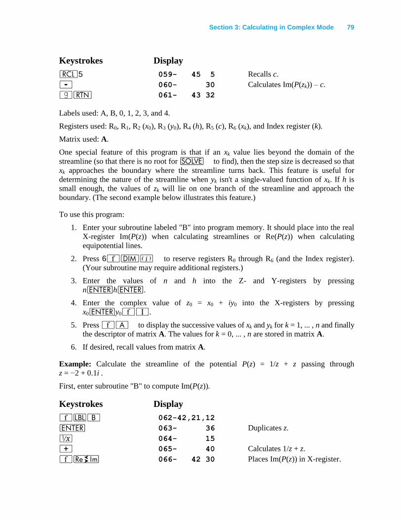
Section 3: Calculating in Complex Mode 79
Keystrokes Display
l5 059- 45 5 Recalls c.
- 060- 30 Calculates Im(P(zk)) – c.
|n 061- 43 32
Labels used: A, B, 0, 1, 2, 3, and 4.
Registers used: R0, R1, R2 (x0), R3 (y0), R4 (h), R5 (c), R6 (xk), and Index register (k).
Matrix used: A.
One special feature of this program is that if an xk value lies beyond the domain of the
streamline (so that there is no root for _ to find), then the step size is decreased so that
xk approaches the boundary where the streamline turns back. This feature is useful for
determining the nature of the streamline when yk isn't a single-valued function of xk. If h is
small enough, the values of zk will lie on one branch of the streamline and approach the
boundary. (The second example below illustrates this feature.)
To use this program:
1. Enter your subroutine labeled "B" into program memory. It should place into the real
X-register Im(P(z)) when calculating streamlines or Re(P(z)) when calculating
equipotential lines.
2. Press 6´m% to reserve registers R0 through R6 (and the Index register).
(Your subroutine may require additional registers.)
3. Enter the values of n and h into the Z- and Y-registers by pressing
nvhv.
4. Enter the complex value of z0 = x0 + iy0 into the X-registers by pressing
x0vy0´V.
5. Press ´A to display the successive values of xk and yk for k = 1, ... , n and finally
the descriptor of matrix A. The values for k = 0, ... , n are stored in matrix A.
6. If desired, recall values from matrix A.
Example: Calculate the streamline of the potential P(z) = 1/z + z passing through
z = −2 + 0.1i .
First, enter subroutine "B" to compute Im(P(z)).
Keystrokes Display
´bB 062-42,21,12
v 063- 36 Duplicates z.
⁄ 064- 15
+ 065- 40 Calculates 1/z + z.
´} 066- 42 30 Places Im(P(z)) in X-register.
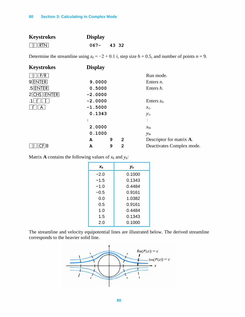
80 Section 3: Calculating in Complex Mode
80
Keystrokes Display
|n 067- 43 32
Determine the streamline using z0 = −2 + 0.1 i, step size h = 0.5, and number of points n = 9.
Keystrokes Display
|¥ Run mode.
9v 9.0000 Enters n.
.5v 0.5000 Enters h.
2”v -2.0000
.1´V -2.0000 Enters z0.
´A -1.5000 x1.
0.1343 y1.
⋮ ⋮
2.0000 x9.
0.1000 y9.
A 9 2 Descriptor for matrix A.
|"8 A 9 2 Deactivates Complex mode.
Matrix A contains the following values of xk and yk:
xk yk
−2.0 0.1000
−1.5 0.1343
−1.0 0.4484
−0.5 0.9161
0.0 1.0382
0.5 0.9161
1.0 0.4484
1.5 0.1343
2.0 0.1000
The streamline and velocity equipotential lines are illustrated below. The derived streamline
corresponds to the heavier solid line.
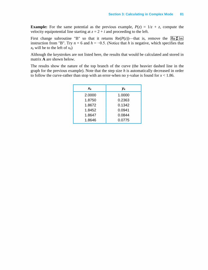
Section 3: Calculating in Complex Mode 81
Example: For the same potential as the previous example, P(z) = 1/z + z, compute the
velocity equipotential line starting at z = 2 + i and proceeding to the left.
First change subroutine "B" so that it returns Re(P(z))—that is, remove the } instruction from "B". Try n = 6 and h = −0.5. (Notice that h is negative, which specifies that
xk will be to the left of x0)
Although the keystrokes are not listed here, the results that would be calculated and stored in
matrix A are shown below.
The results show the nature of the top branch of the curve (the heavier dashed line in the
graph for the previous example). Note that the step size h is automatically decreased in order
to follow the curve-rather than stop with an error-when no y-value is found for x < 1.86.
xk yk
2.0000 1.0000
1.8750 0.2363
1.8672 0.1342
1.8452 0.0941
1.8647 0.0844
1.8646 0.0775
82
Section 4: Using Matrix Operations
Matrix algebra is a powerful tool. It allows you to more easily formulate and solve many
complicated problems, simplifying otherwise intricate computations. In this section you will
find information about how the HP-15C performs certain matrix operations and about using
matrix operations in your applications.
Several results from numerical linear algebra theory are summarized in this section. This
material is not meant to be self-contained. You may want to consult a reference for more
complete presentations.**
Understanding the LU Decomposition
The HP-15C can solve systems of linear equations, invert matrices, and calculate
determinants. In performing these calculations, the HP-15C transforms a square matrix into a
computationally convenient form called the LU decomposition of the matrix.
The LU decomposition procedure factors a square matrix A into the matrix product LU. L is
a lower-triangular matrix with 1's on its diagonal and with subdiagonal elements (those
below the diagonal) between -1 and +1, inclusive. U is an upper-triangular matrix.††
For
example:
LUA
5.0
32
15.
01
11
32.
Some matrices can't be factored into the LU form. For example,
LUA
21
10
for any pair of lower- and upper-triangular matrices L and U. However, if rows are
interchanged in the matrix to be factored, an LU decomposition can always be constructed.
Row interchanges in the matrix A can be represented by the matrix product PA for some
square matrix P. Allowing for row interchanges, the LU decomposition can be represented by
the equation PA = LU. So for the above example,
LUPA
10
21
10
01
10
21
21
10
01
10.
** Two such references are
Atkinson, Kendall E., An Introduction to Numerical Analysis, Wiley, 1978.
Kahan, W. "Numerical Linear Algebra," Canadian Mathematical Bulletin, Volume 9, 1966, pp. 756-801.
†† A lower-triangular matrix has 0’s for all elements above its diagonal. An uppertriangular matrix has 0's for all elements
below its diagonal.
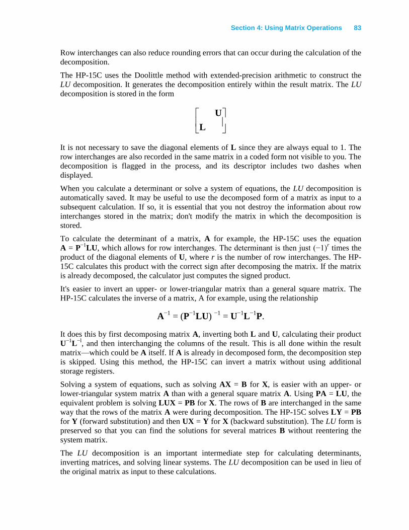
Section 4: Using Matrix Operations 83
Row interchanges can also reduce rounding errors that can occur during the calculation of the
decomposition.
The HP-15C uses the Doolittle method with extended-precision arithmetic to construct the
LU decomposition. It generates the decomposition entirely within the result matrix. The LU
decomposition is stored in the form
L
U
It is not necessary to save the diagonal elements of L since they are always equal to 1. The
row interchanges are also recorded in the same matrix in a coded form not visible to you. The
decomposition is flagged in the process, and its descriptor includes two dashes when
displayed.
When you calculate a determinant or solve a system of equations, the LU decomposition is
automatically saved. It may be useful to use the decomposed form of a matrix as input to a
subsequent calculation. If so, it is essential that you not destroy the information about row
interchanges stored in the matrix; don't modify the matrix in which the decomposition is
stored.
To calculate the determinant of a matrix, A for example, the HP-15C uses the equation
A = P−1
LU, which allows for row interchanges. The determinant is then just (−1)r times the
product of the diagonal elements of U, where r is the number of row interchanges. The HP-
15C calculates this product with the correct sign after decomposing the matrix. If the matrix
is already decomposed, the calculator just computes the signed product.
It's easier to invert an upper- or lower-triangular matrix than a general square matrix. The
HP-15C calculates the inverse of a matrix, A for example, using the relationship
A−1
= (P−1
LU) −1
= U−1
L−1
P.
It does this by first decomposing matrix A, inverting both L and U, calculating their product
U−1
L−l
, and then interchanging the columns of the result. This is all done within the result
matrix—which could be A itself. If A is already in decomposed form, the decomposition step
is skipped. Using this method, the HP-15C can invert a matrix without using additional
storage registers.
Solving a system of equations, such as solving AX = B for X, is easier with an upper- or
lower-triangular system matrix A than with a general square matrix A. Using PA = LU, the
equivalent problem is solving LUX = PB for X. The rows of B are interchanged in the same
way that the rows of the matrix A were during decomposition. The HP-15C solves LY = PB
for Y (forward substitution) and then UX = Y for X (backward substitution). The LU form is
preserved so that you can find the solutions for several matrices B without reentering the
system matrix.
The LU decomposition is an important intermediate step for calculating determinants,
inverting matrices, and solving linear systems. The LU decomposition can be used in lieu of
the original matrix as input to these calculations.
84 Section 4: Using Matrix Operations
84
ILL-Conditioned Matrices and the Condition Number
In order to discuss errors in matrix calculations, it's useful to define a measure of distance
between two matrices. One measure of the distance between matrices A and B is the norm of
their difference, denoted ||A − B||. The norm can also be used to define the condition number
of a matrix, which indicates how the relative error of a calculation compares to the relative
error of the matrix itself.
The HP-15C provides three norms. The Frobenius norm of a matrix A, denoted ||A||F, is the
square root of the sum of the squares of the matrix elements. This is the matrix analog of the
Euclidean length of a vector.
Another norm provided by the HP-15C is the row norm. The row norm of an m n matrix A
is the largest row sum of absolute values and is denoted ||A||R:
n
j
ijRa
mi 11
maxA
The column norm of the matrix is denoted ||A||C and can be computed by ||A||C = ||AT||R. The
column norm is the largest column sum of absolute values.
For example, consider the matrices
654
222and
954
321BA
Then
300
101BA
and
||A + B||F = 3.311 (Frobenius norm),
||A − B||R = 3 (row norm), and
||A − B||C = 4 (column norm).
The remainder of this discussion assumes that the row norm is used. Similar results are
obtained if any of the other norms is used instead.
The condition number of a square matrix A is defined as
K(A) = ||A|| ||A−1
||.
Then 1 ≤ K(A) < ∞ using any norm. The condition number is useful for measuring errors in
calculations. A matrix is said to be ill-conditioned if K(A) is very large.
If rounding or other errors are present in matrix elements, these errors will propagate through
subsequent matrix calculations. They can be magnified significantly. For example, suppose
Section 4: Using Matrix Operations 85
that X and B are nonzero vectors satisfying AX = B for some square matrix A. Suppose A is
perturbed by ΔA and we compute B + ΔB = (A + ΔA)X. Then
)(AAΔA
BΔBK ,
with equality for some perturbation ΔA. This measures how much the relative uncertainty in
A can be magnified when propagated into the product.
The condition number also measures how much larger in norm the relative uncertainty of the
solution to a system can be compared to that of the stored data. Suppose again that X and B
are nonzero vectors satisfying AX = B for some matrix A. Suppose now that matrix B is
perturbed (by rounding errors, for example) by an amount ΔB. Let X + ΔX satisfy
A(X + ΔX) = B +ΔB. Then
)(ABΔB
XΔXK
with equality for some perturbation ΔB.
Suppose instead that matrix A is perturbed by ΔA. Let X + ΔX satisfy (A + ΔA)(X + ΔX) =
B. If d(A, ΔA) = K(A)||ΔA|| /||A|| < 1, then
)(1
)(
ΔAA,
A
AΔA
XΔX
d
K
.
Similarly, if A−1
+ Z is the inverse of the perturbed matrix A + ΔA, then
)(1
)(
ΔAA,
A
AΔA
AZ 1
d
K
.
Moreover, certain perturbations ΔA cause the inequalities to become equalities.
All of the preceding relationships show how the relative error of the result is related to the
relative error of matrix A via the condition number K(A). For each inequality, there are
matrices for which equality is true. A large condition number makes possible a relatively
large error in the result.
Errors in the data—sometimes very small relative errors—can cause the solution of an ill-
conditioned system to be quite different from the solution of the original system. In the same
way, the inverse of a perturbed ill-conditioned matrix can be quite different from the inverse
of the unperturbed matrix. But both differences are bounded by the condition number; they
can be relatively large only if the condition number K(A) is large.
Also, a large condition number K(A) of a nonsingular matrix A indicates that the matrix A is
relatively close, in norm, to a singular matrix. That is
86 Section 4: Using Matrix Operations
86
ASAA min)(1 K
and
SAA1 min1 ,
where the minimum is taken over all singular matrices S. That is, if K(A) is large, then the
relative difference between A and the closest singular matrix S is small. If the norm of A−1
is
large, the difference between A and the closest singular matrix S is small.
For example, let
9999999999.1
11A
Then
1010
10
1010
10999,999,999,91A
and ||A−1
|| = 2 × 10¹⁰
. Therefore, there should exist a perturbation ΔA with ||ΔA|| = 5 ×10⁻¹¹
that makes A + ΔA singular. Indeed, if
11
11
1050
1050ΔA
with ||ΔA|| = 5 ×10⁻¹¹
, then
59999999999.1
59999999999.1ΔAA
and A + ΔA is singular.
The figures below illustrate these ideas. In each figure matrix A and matrix S are shown
relative to the "surface" of singular matrices and within the space of all matrices. Distance is
measured using the norm. Around every matrix A is a region of matrices that are practically
indistinguishable from A (for example, those within rounding errors of A). The radius of this
region is ||ΔA||. The distance from a nonsingular matrix A to the nearest singular matrix S is
1/||A−1
||.
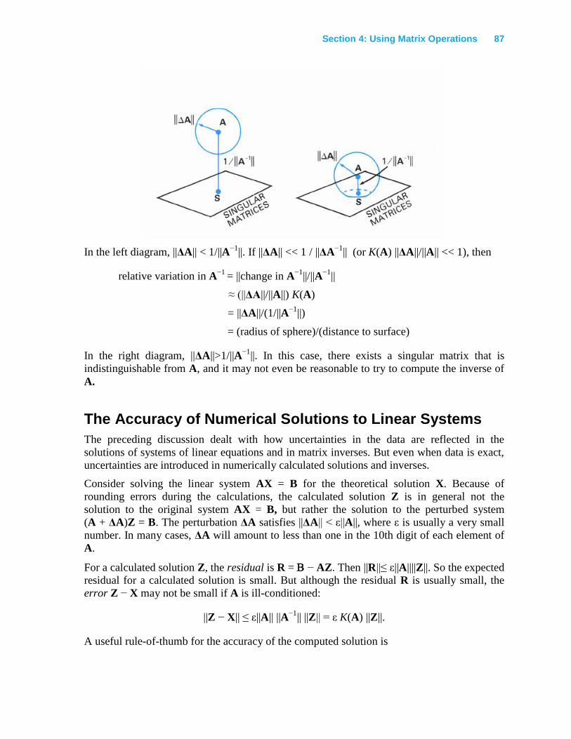
Section 4: Using Matrix Operations 87
In the left diagram, ||ΔA|| < 1/||A−1
||. If ||ΔA|| << 1 / ||ΔA−1
|| (or K(A) ||ΔA||/||A|| << 1), then
relative variation in A−1
= ||change in A−1
||/||A−1
||
≈ (||ΔA||/||A||) K(A)
= ||ΔA||/(1/||A−1
||)
= (radius of sphere)/(distance to surface)
In the right diagram, ||ΔA||>1/||A−1
||. In this case, there exists a singular matrix that is
indistinguishable from A, and it may not even be reasonable to try to compute the inverse of
A.
The Accuracy of Numerical Solutions to Linear Systems
The preceding discussion dealt with how uncertainties in the data are reflected in the
solutions of systems of linear equations and in matrix inverses. But even when data is exact,
uncertainties are introduced in numerically calculated solutions and inverses.
Consider solving the linear system AX = B for the theoretical solution X. Because of
rounding errors during the calculations, the calculated solution Z is in general not the
solution to the original system AX = B, but rather the solution to the perturbed system
(A + ΔA)Z = B. The perturbation ΔA satisfies ||ΔA|| < ε||A||, where ε is usually a very small
number. In many cases, ΔA will amount to less than one in the 10th digit of each element of
A.
For a calculated solution Z, the residual is R = − AZ. Then ||R||≤ ε||A||||Z||. So the expected
residual for a calculated solution is small. But although the residual R is usually small, the
error Z − X may not be small if A is ill-conditioned:
||Z − X|| ≤ ε||A|| ||A−1
|| ||Z|| = ε K(A) ||Z||.
A useful rule-of-thumb for the accuracy of the computed solution is
88 Section 4: Using Matrix Operations
88
)10log(logcarrieddigits
ofnumber
digits decimal
correctofnumbern
1AA
where n is the dimension of A. For the HP-15C, which carries 10 accurate digits,
(number of correct decimal digits) ≥ 9 − log(||A|| ||A−1
||) − log(10n).
In many applications, this accuracy may be adequate. When additional accuracy is desired,
the computed solution Z can usually be improved by iterative refinement (also known as
residual correction).
Iterative refinement involves calculating a solution to a system of equations, then improving
its accuracy using the residual associated with the solution to modify that solution.
To use iterative refinement, first calculate a solution Z to the original system AX = B. Z is
then treated as an approximation to X, in error by E = X − Z. Then E satisfies the linear
system AE = AX − AZ = R, where R is the residual for Z. The next step is to calculate the
residual and then to solve AE = R for E. The calculated solution, denoted by F, is treated as
an approximation to E = X − Z and is added to Z to obtain a new approximation to X:
F + Z ≈ (X − Z) + Z = X.
In order for F + Z to be a better approximation to X than is Z, the residual R = B − AZ must
be calculated to extended precision. The HP-15C's >6 operation does this. The system
matrix A is used for finding both solutions, Z and F. The LU decomposition formed while
calculating Z can be used for calculating F, thereby shortening the execution time. The
refinement process can be repeated, but most of the improvement occurs in the first
refinement.
(Refer to Applications at the end of this section for a program that performs one iteration of
refinement.)
Making Difficult Equations Easier
A system of equations EX = B is difficult to numerically solve accurately if E is ill-
conditioned (nearly singular). Even iterative refinement can fail to improve the calculated
solution when E is sufficiently ill-conditioned. However, instances arise in practice when a
modest extra effort suffices to change difficult equations into others with the same solution,
but which are easier to solve. Scaling and preconditioning are two processes to do this.
Scaling
Bad scaling is a common cause of poor results from attempts to numerically invert ill-
conditioned matrices or to solve systems of equations with ill-conditioned system matrices.
But it is a cause that you can easily diagnose and cure.
Suppose a matrix E is obtained from a matrix A by E = LAR, where L and R are scaling
diagonal matrices whose diagonal elements are all integer powers of 10. Then E is said to be
obtained from A by scaling. L scales the rows of A, and R scales the columns. Presumably
E−1
= R−1
A−1
L−1
can be obtained either from A−1
by scaling or from E by inverting.

Section 4: Using Matrix Operations 89
For example, let matrix A be
112
111
21103 40
A .
The HP-15C correctly calculates A−1
to 10-digit accuracy as
121
243
1321
A .
Now let
20
20
20
1000
0100
0010
RL
so that
4040
4040
10102
10101
213
E .
E is very near a singular matrix
002
001
213
S
and ||E – S|| / ||E|| = ⅓ × 10–40
. This means that K(S) ≥ 3 × 1040
, so it's not surprising that the
calculated E–1
99
99
1011
10142.210284.407155.0
10284.410569.88569.0
1011067.61
E
is far from the true value
4040
4040
40
101021
1021043
131021
E
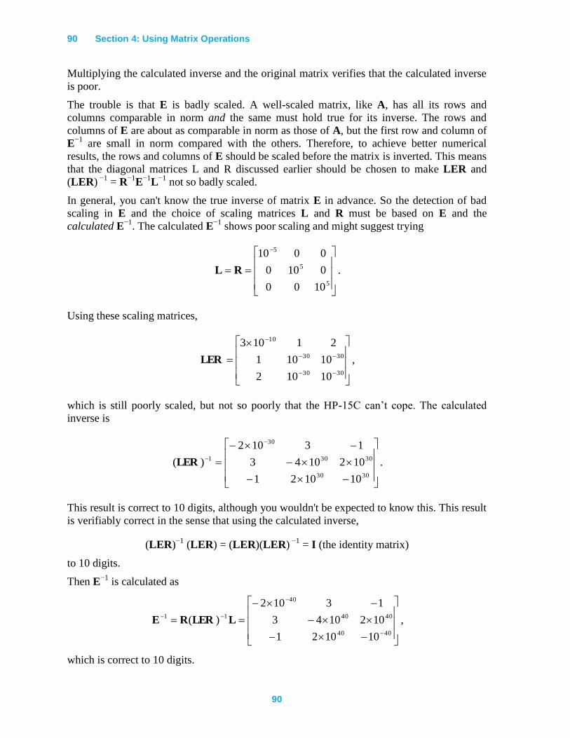
90 Section 4: Using Matrix Operations
90
Multiplying the calculated inverse and the original matrix verifies that the calculated inverse
is poor.
The trouble is that E is badly scaled. A well-scaled matrix, like A, has all its rows and
columns comparable in norm and the same must hold true for its inverse. The rows and
columns of E are about as comparable in norm as those of A, but the first row and column of
E−1
are small in norm compared with the others. Therefore, to achieve better numerical
results, the rows and columns of E should be scaled before the matrix is inverted. This means
that the diagonal matrices L and R discussed earlier should be chosen to make LER and
(LER) −1
= R−1
E−1
L−1
not so badly scaled.
In general, you can't know the true inverse of matrix E in advance. So the detection of bad
scaling in E and the choice of scaling matrices L and R must be based on E and the
calculated E−1
. The calculated E−1
shows poor scaling and might suggest trying
5
5
5
1000
0100
0010
RL .
Using these scaling matrices,
3030
3030
10
10102
10101
21103
LER ,
which is still poorly scaled, but not so poorly that the HP-15C can’t cope. The calculated
inverse is
3030
3030
30
1
101021
1021043
13102
)(LER .
This result is correct to 10 digits, although you wouldn't be expected to know this. This result
is verifiably correct in the sense that using the calculated inverse,
(LER)−1
(LER) = (LER)(LER) −1
= I (the identity matrix)
to 10 digits.
Then E−1
is calculated as
4040
4040
40
11
101021
1021043
13102
)( LLERRE ,
which is correct to 10 digits.
Section 4: Using Matrix Operations 91
If (LER) −1
is verifiably poor, you can repeat the scaling, using LER in place of E and using
new scaling matrices suggested by LER and the calculated (LER)−1
.
You can also apply scaling to solving a system of equations, for example EX = B, where E is
poorly scaled. When solving for X, replace the system EX = B by a system (LER)Y = LB to
be solved for Y. The diagonal scaling matrices L and R are chosen as before to make the
matrix LER well-scaled. After you calculate Y from the new system, calculate the desired
solution as X = RY.
Preconditioning
Preconditioning is another method by which you can replace a difficult system, EX = B, by
an easier one, AX = D, with the same solution X.
Suppose that E is ill-conditioned (nearly singular). You can detect this by calculating the
inverse E−1
and observing that 1/||E−1
|| is very small compared to ||E|| (or equivalently by a
large condition number K(E)). Then almost every row vector uT will have the property that
||uT||/||u
T E
−1|| is also very small compared with ||E||, where E
−1 is the calculated inverse. This
is because most row vectors uT will have ||u
T E
−1|| not much smaller than ||u
T|| ||E
−1||, and
||E−1
|| will be large. Choose such a row vector uT and calculate v
T = au
TE
−1. Choose the scalar
a so that the row vector rT, obtained by rounding every element of v
T to an integer between
−100 and 100, does not differ much from vT. Then r
T is a row vector with integer elements
with magnitudes less than 100. ||rTE|| will be small compared with ||r
T|| ||E||—the smaller the
better.
Next, choose the kth element of rT having one of the largest magnitudes. Replace the kth row
of E by rTE and the kth row of B by r
TB. Provided that no roundoff has occurred during the
evaluation of these new rows, the new system matrix A should be better conditioned (farther
from singular) than E was, but the system will still have the same solution X as before.
This process works best when E and A are both scaled so that every row of E and of A have
roughly the same norm as every other. You can do this by multiplying the rows of the
systems of equations EX = B and AX = D by suitable powers of 10. If A is not far enough
from singular, though well scaled, repeat the preconditioning process.
As an illustration of the preconditioning process, consider the system EX = B, where
0
0
0
0
1
, BE
xyyyy
yxyyy
yyxyy
yyyxy
yyyyx
and x = 8000.00002 and y = −1999.99998. If you attempt to solve this system directly, the
HP-15C calculates the solution X and the inverse E−1
to be
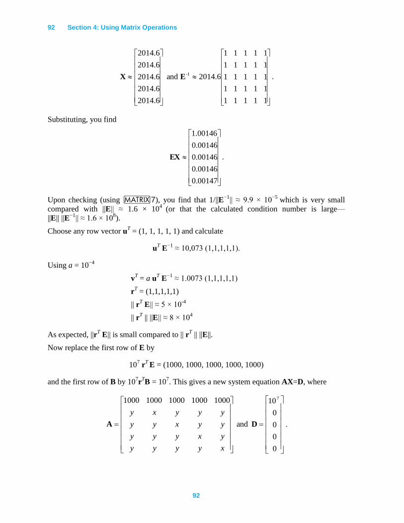
92 Section 4: Using Matrix Operations
92
11111
11111
11111
11111
11111
6.2014and
6.2014
6.2014
6.2014
6.2014
6.2014
1-EX .
Substituting, you find
00147.0
00146.0
00146.0
00146.0
00146.1
EX .
Upon checking (using >7), you find that 1/||E−1
|| ≈ 9.9 × 10⁻⁵
which is very small
compared with ||E|| ≈ 1.6 × 10⁴
(or that the calculated condition number is large—
||E|| ||E−1
|| ≈ 1.6 × 10⁸).
Choose any row vector uT = (1, 1, 1, 1, 1) and calculate
uT E
−1 ≈ 10,073 (1,1,1,1,1).
Using a = 10−4
vT = a u
T E
−1 ≈ 1.0073 (1,1,1,1,1)
rT = (1,1,1,1,1)
|| rT E|| ≈ 5 × 10
-4
|| rT || ||E|| ≈ 8 × 10
4
As expected, ||rT E|| is small compared to || r
T || ||E||.
Now replace the first row of E by
107 r
T E = (1000, 1000, 1000, 1000, 1000)
and the first row of B by 107r
TB = 10
7. This gives a new system equation AX=D, where
0
0
0
0
10
and
10001000100010001000 7
DA
xyyyy
yxyyy
yyxyy
yyyxy
.
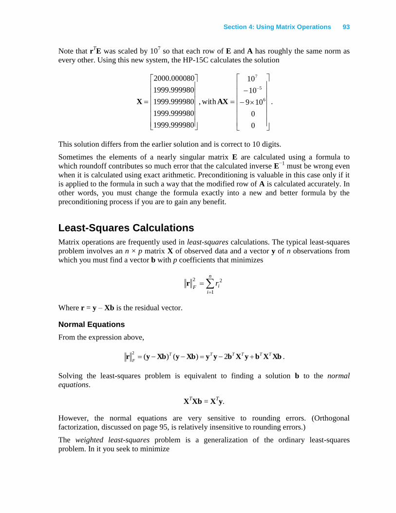
Section 4: Using Matrix Operations 93
Note that rTE was scaled by 10
7 so that each row of E and A has roughly the same norm as
every other. Using this new system, the HP-15C calculates the solution
0
0
109
10
10
with,
999980.1999
999980.1999
999980.1999
999980.1999
000080.2000
6
5
7
AXX .
This solution differs from the earlier solution and is correct to 10 digits.
Sometimes the elements of a nearly singular matrix E are calculated using a formula to
which roundoff contributes so much error that the calculated inverse E−1
must be wrong even
when it is calculated using exact arithmetic. Preconditioning is valuable in this case only if it
is applied to the formula in such a way that the modified row of A is calculated accurately. In
other words, you must change the formula exactly into a new and better formula by the
preconditioning process if you are to gain any benefit.
Least-Squares Calculations
Matrix operations are frequently used in least-squares calculations. The typical least-squares
problem involves an n × p matrix X of observed data and a vector y of n observations from
which you must find a vector b with p coefficients that minimizes
n
i
iFr
1
22r
Where r = y – Xb is the residual vector.
Normal Equations
From the expression above,
XbXbyXbyyXbyXbyrTTTTTT
F 2)()(
2.
Solving the least-squares problem is equivalent to finding a solution b to the normal
equations.
XTXb = X
Ty.
However, the normal equations are very sensitive to rounding errors. (Orthogonal
factorization, discussed on page 95, is relatively insensitive to rounding errors.)
The weighted least-squares problem is a generalization of the ordinary least-squares
problem. In it you seek to minimize
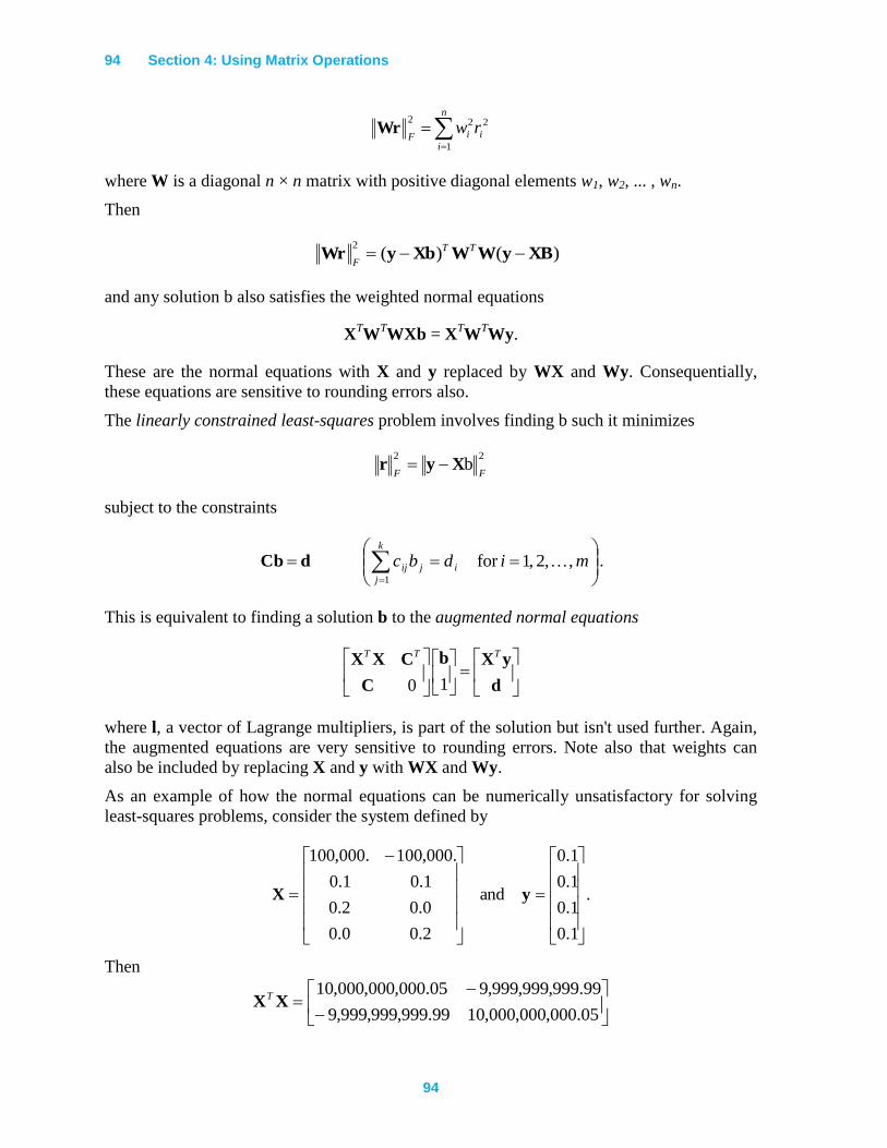
94 Section 4: Using Matrix Operations
94
n
i
iiFrw
1
222Wr
where W is a diagonal n × n matrix with positive diagonal elements w1, w2, ... , wn.
Then
)()(2
XByWWXbyWr TT
F
and any solution b also satisfies the weighted normal equations
XTW
TWXb = X
TW
TWy.
These are the normal equations with X and y replaced by WX and Wy. Consequentially,
these equations are sensitive to rounding errors also.
The linearly constrained least-squares problem involves finding b such it minimizes
22b
FFXyr
subject to the constraints
k
j
ijij midbc1
,,2,1for dCb .
This is equivalent to finding a solution b to the augmented normal equations
d
yXb
C
CXXTTT
10
where l, a vector of Lagrange multipliers, is part of the solution but isn't used further. Again,
the augmented equations are very sensitive to rounding errors. Note also that weights can
also be included by replacing X and y with WX and Wy.
As an example of how the normal equations can be numerically unsatisfactory for solving
least-squares problems, consider the system defined by
.
1.0
1.0
1.0
1.0
and
2.00.0
0.02.0
1.01.0
.000,100.000,100
yX
Then
05.000,000,000,1099.999,999,999,9
99.999,999,999,905.000,000,000,10XX
T
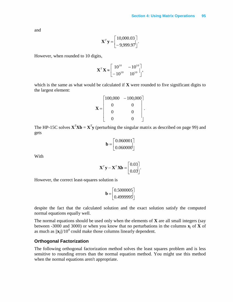
Section 4: Using Matrix Operations 95
and
.97.999,9
03.000,10
yX
T
However, when rounded to 10 digits,
,1010
10101010
1010
XX
T
which is the same as what would be calculated if X were rounded to five significant digits to
the largest element:
.
00
00
00
000,100000,100
X
The HP-15C solves XTXb = X
Ty (perturbing the singular matrix as described on page 99) and
gets
060000.0
060001.0b
With
.03.0
03.0
XbXyX
TT
However, the correct least-squares solution is
4999995.0
5000005.0b
despite the fact that the calculated solution and the exact solution satisfy the computed
normal equations equally well.
The normal equations should be used only when the elements of X are all small integers (say
between -3000 and 3000) or when you know that no perturbations in the columns xj of X of
as much as ||xj||/104 could make those columns linearly dependent.
Orthogonal Factorization
The following orthogonal factorization method solves the least squares problem and is less
sensitive to rounding errors than the normal equation method. You might use this method
when the normal equations aren't appropriate.
96 Section 4: Using Matrix Operations
96
Any n × p matrix X can be factored as X = QTU, where Q is an n × n orthogonal matrix
characterized by QT = Q
−l and U is an n × p upper-triangular matrix. The essential property
of orthogonal matrices is that they preserve length in the sense that
.
)r()(
2
2
F
T
TT
T
F
r
rr
QrQr
QQrrQ
Therefore, if r = y – Xb, it has the same length as
Qr = Qy – QXb = Qy – Ub.
The upper-triangular matrix U and the product Qy can be written as
.rows)(
rows)(and
rows)(
rows)(ˆ
pn
p
pn
p
f
gQy
O
UU
Then
2
22
2
22
ˆ
r
F
FF
F
FF
f
fbUg
UbQy
Qr
with equality when 0bUg ˆ . In other words, the solution to the ordinary least-squares
problem is any solution to gbU ˆ and the minimal sum of squares is 2
Ff . This is the basis
of all numerically sound least-squares programs.
You can solve the unconstrained least-squares problem in two steps:
1. Perform the orthogonal factorization of the augmented n × (p + 1) matrix
VQyXT
where QT = Q
−1, and retain only the upper-triangular factor V, which you can then
partition as
rows)1(
row)(1
rows)(ˆ
pn
p
q
00
0
gU
V
(1 column)
(p columns)
Section 4: Using Matrix Operations 97
Only the first p + 1 rows (and columns) of V need to be retained. (Note that Q here is
not the same as that mentioned earlier, since this Q must also transform y.)
2. Solve the following system for b:
.1
ˆ
0b
0
gU
(If q = 0, replace it by any small nonzero number, say 10−99
.) The −1 in the solution
matrix automatically appears; it requires no additional calculations.
In the absence of rounding errors, q = ±||y – Xb||F; this may be inaccurate if |q| is too
small, say smaller than ||y||/l06. If you desire a more accurate estimate of ||y – Xb||F,
you can calculate it directly from X, y, and the computed solution b.
For the weighted least-squares problem, replace X and y by WX and Wy, where W is the
diagonal matrix containing the weights.
For the linearly constrained least-squares problem, you must recognize that constraints may
be inconsistent. In addition, they can't always be satisfied exactly by a calculated solution
because of rounding errors. Therefore, you must specify a tolerance t such that the constraints
are said to be satisfied when ||Cb – d|| < t. Certainly t > ||d||/1010
for 10-digit computation,
and in some cases a much larger tolerance must be used.
Having chosen t, select a weight factor w that satisfies w > ||y||/t. For convenience, choose w
to be a power of 10 somewhat bigger than ||y||/t. Then w||Cb – d|| > ||y|| unless ||Cb – d|| < t.
However, the constraint may fail to be satisfied for one of two reasons:
No b exists for which ||Cb – d|| < t.
The leading columns of C are nearly linearly dependent.
Check for the first situation by determining whether a solution exists for the constraints
alone. When [wC wd] has been factored to Q[U g], solve this system for b
)row1(
)rows(
1)diag()rows1(
)rows( p
qqkp
k
0b
0
gU
using any small nonzero number q. If the computed solution b satisfies Cb ≈ d, then the
constraints are not inconsistent.
The second situation is rarely encountered and can be avoided. It shows itself by causing at
least one of the diagonal elements of U to be much smaller than the largest element above it
in the same column, where U is from the orthogonal factorization wC = QU.
To avoid this situation, reorder the columns of wC and X and similarly reorder the elements
(rows) of b. The reordering can be chosen easily if the troublesome diagonal element of U is
also much smaller than some subsequent element in its row. Just swap the corresponding
98 Section 4: Using Matrix Operations
98
columns in the original data and refactor the weighted constraint equations. Repeat this
procedure if necessary.
For example, if the factorization of wC gives
2.15.15.200
1.00.35.002.00
3.05.15.00.20.1
U ,
then the second diagonal element is much smaller than the value 2.0 above it. This indicates
that the first and second columns in the original constraints are nearly dependent. The
diagonal element is also much smaller than the subsequent value 3.0 in its row. Then the
second and fourth columns should be swapped in the original data and the factorization
repeated.
It is always prudent to check for consistent constraints. The test for small diagonal elements
of U can be done at the same time.
Finally, using U and g as the first k rows, add rows corresponding to X and y. (Refer to
Least-Squares Using Successive Rows on page 118 for additional information.) Then solve
the unconstrained least-squares problem with
y
dy
X
CX
wwand .
Provided the calculated solution b satisfies ||Cb – d|| < t, that solution will also minimize ||y –
Xb|| subject to the constraint Cb ≈ d.
Singular and Nearly Singular Matrices
A matrix is singular if and only if its determinant is zero. The determinant of a matrix is
equal to (−1)r times the product of the diagonal elements of U, where U is the upper-diagonal
matrix of the matrix's LU decomposition and r is the number of row interchanges in the
decomposition. Then, theoretically, a matrix is singular if at least one of the diagonal
elements of U, the pivots, is zero; otherwise it is nonsingular.
However, because the HP-15C performs calculations with only a finite number of digits,
some singular and nearly singular matrices can't be distinguished in this way. For example,
consider the matrix
LUB
00
33
1
01
11
33
31
,
which is singular. Using 10-digit accuracy, this matrix is decomposed as
Section 4: Using Matrix Operations 99
10100
33
13333333333.
01LU ,
which is nonsingular. The singular matrix B can't be distinguished from the nonsingular
matrix
19999999999.
33D
since they both have identical calculated LU decompositions.
On the other hand, the matrix
LUA
103
1 100
33
1
01
9999999999.1
33
is nonsingular. Using 10-digit accuracy, matrix A is decomposed as
00
33
13333333333.
01LU .
This would incorrectly indicate that matrix A is singular. The nonsingular matrix A can't be
distinguished from the singular matrix
9999999999.9999999999.
33C
since they both have identical calculated LU decompositions.
When you use the HP-15C to calculate an inverse or to solve a system of equations, you
should understand that some singular and nearly singular matrices have the same calculated
LU decomposition. For this reason, the HP-15C always calculates a result by ensuring that all
decomposed matrices never have zero pivots. It does this by perturbing the pivots, if
necessary, by an amount that is usually smaller than the rounding error in the calculations.
This enables you to invert matrices and solve systems of equations without being interrupted
by zero pivots. This is very important in applications such as calculating eigenvectors using
the method of inverse iteration (refer to page 130).
The effect of rounding errors and possible intentional perturbations is to cause the calculated
decomposition to have all nonzero pivots and to correspond to a nonsingular matrix A + ΔA
usually identical to or negligibly different from the original matrix A. Specifically, unless
every element in some column of A has absolute value less than 10−89
, the column sum norm
||ΔA||C will be negligible (to 10 significant digits) compared with ||A||C.
The HP-15C calculates the determinant of a square matrix as the signed product of the
(possibly perturbed) calculated pivots. The calculated determinant is the determinant of the
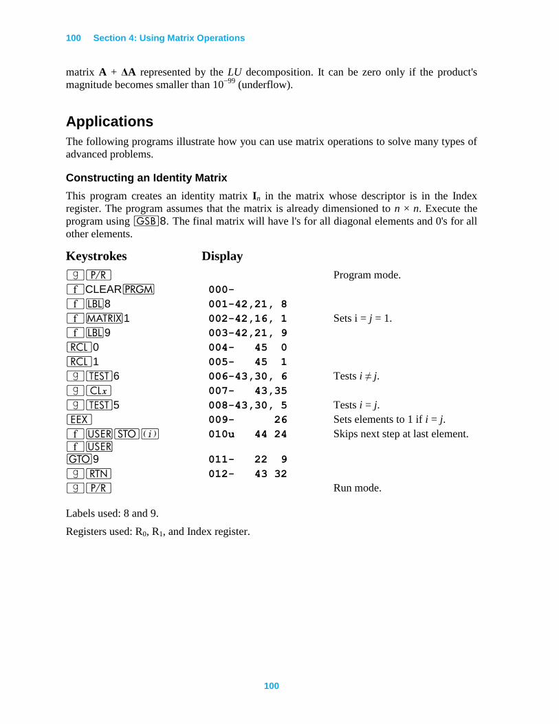
100 Section 4: Using Matrix Operations
100
matrix A + ΔA represented by the LU decomposition. It can be zero only if the product's
magnitude becomes smaller than 10−99
(underflow).
Applications
The following programs illustrate how you can use matrix operations to solve many types of
advanced problems.
Constructing an Identity Matrix
This program creates an identity matrix In in the matrix whose descriptor is in the Index
register. The program assumes that the matrix is already dimensioned to n × n. Execute the
program using G8. The final matrix will have l's for all diagonal elements and 0's for all
other elements.
Keystrokes Display
|¥ Program mode.
´CLEARM 000-
´b8 001-42,21, 8
´>1 002-42,16, 1 Sets i = j = 1.
´b9 003-42,21, 9
l0 004- 45 0
l1 005- 45 1
|T6 006-43,30, 6 Tests i ≠ j.
|` 007- 43,35
|T5 008-43,30, 5 Tests i = j.
“ 009- 26 Sets elements to 1 if i = j.
´UO% ´U
010u 44 24 Skips next step at last element.
t9 011- 22 9
|n 012- 43 32
|¥ Run mode.
Labels used: 8 and 9.
Registers used: R0, R1, and Index register.
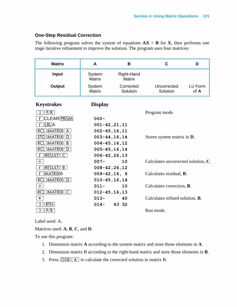
Section 4: Using Matrix Operations 101
One-Step Residual Correction
The following program solves the system of equations AX = B for X, then performs one
stage iterative refinement to improve the solution. The program uses four matrices:
Matrix A B C D
Input System Matrix
Right-Hand Matrix
Output System Matrix
Corrected Solution
Uncorrected Solution
LU Form of A
Keystrokes Display
|¥ Program mode.
´CLEARM 000-
´bA 001-42,21,11
l>A 002-45,16,11
O>Á 003-44,16,14 Stores system matrix in D.
l>B 004-45,16,12
l>Á 005-45,16,14
´<C 006-42,26,13
÷ 007- 10 Calculates uncorrected solution, C.
´<B 008-42,26,12
´>6 009-42,16, 6 Calculates residual, B.
l>Á 010-45,16,14
÷ 011- 10 Calculates correction, B.
l>C 012-45,16,13
+ 013- 40 Calculates refined solution, B.
|n 014- 43 32
|¥ Run mode.
Label used: A.
Matrices used: A, B, C, and D.
To use this program:
1. Dimension matrix A according to the system matrix and store those elements in A.
2. Dimension matrix B according to the right-hand matrix and store those elements in B.
3. Press GA to calculate the corrected solution in matrix B.
102 Section 4: Using Matrix Operations
102
Example: Use the residual correction program to calculate the inverse of matrix A for
.
1748
571024
721633
A
The theoretical inverse of A is
.
93/23/8
2/512/58
323/83/291
A
Find the inverse by solving AX = B for X, where B is a 3 × 3 identity matrix.
First, enter the program from above. Then, in Run mode, enter the elements into matrix A
(the system matrix) and matrix B (the right-hand, identity matrix). Press GA to
execute the program.
Recall the elements of the uncorrected solution, matrix C:
.
000000203.96666666836.0666666728.2
50000055.25500000046.2000000167.8
00000071.32666666726.2666666881.9
C
This solution is correct to seven digits. The accuracy is well within that predicted by the
equation on page 88.
(number of correct digits) ≥ 9 – log(||A|| ||C||) – log (3) ≈ 4.8.
Recall the elements of the corrected solution, matrix B:
.
000000000.96666666667.0666666667.2
50000000.25500000000.2000000000.8
00000000.32666666667.2666666667.9
B
One iteration of refinement yields 10 correct digits in this case.
Solving a System of Nonlinear Equations
Consider a system of p nonlinear equations in p unknowns:
fi(x1, x2, …, xp) = 0 for i = 1, 2, …, p
for which the solution x1, x2, … , xp is sought.
Section 4: Using Matrix Operations 103
Let
)()(
)()(
)()(
)(and,
)(
)(
)(
)(,
1
221
111
2
1
2
1
xx
xx
xx
xF
x
x
x
xfx
ppp
p
p
pp FF
FF
FF
f
f
f
x
x
x
,
where
)()( xx i
j
ij fx
F
for i, j = 1, 2, …, p.
The system of equations can be expressed as f(x) = 0. Newton's method starts with an initial
guess x(0)
to a root x of f(x) = 0 and calculates
x(k + 1)
= x(k)
− (F(x(k)
))−1
f(x(k)
) for k = 0, 1, 2, …
until x(k+1)
converges.
The program in the following example performs one iteration of Newton's method. The
computations are performed as
x(k + 1)
= x(k)
− d(k)
,
where d(k)
is the solution to the p×p linear system
F(x(k)
)d(k)
= f(x(k)
) .
The program displays the Euclidean lengths of f(x(k)
) and the correction d(k)
at the end of each
iteration.
Example: For the random variable y having a normal distribution with unknown mean m and
variance v2, construct an unbiased test of the hypothesis that 2
02 vv versus the alternative that
20
2 vv for a particular value 20v .
For a random sample of y consisting of y1, y2, … , yn an unbiased test rejects the hypothesis if
2
02
2
01 vxsorvxs nn ,
where
n
i
i
n
i
in yn
yandyys11
2 1)(
for some constants x1 and x2.
If the size of the test is a (0 < a < 1), you can find xl and x2 by solving the system of
equations f1(x) = f2(x) = 0, where
f1(x) = (n – 1) ln(x2 / x1) + x1 – x2
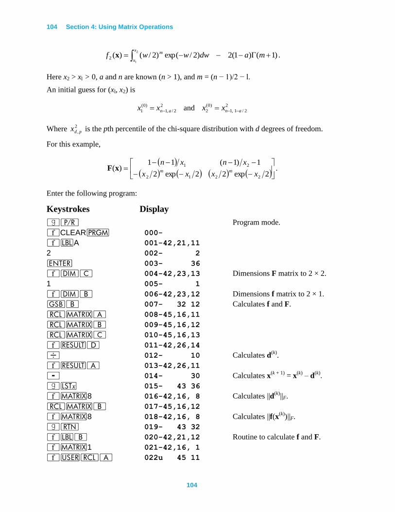
104 Section 4: Using Matrix Operations
104
2
1
)1()1(2)2/exp()2/()(2
x
x
m madwwwf x .
Here x2 > xl > 0, a and n are known (n > 1), and m = (n − 1)/2 − l.
An initial guess for (xl, x2) is
2
2/,1
)0(
1 anxx and 2
2/1,1
)0(
2 anxx
Where 2
, pdx is the pth percentile of the chi-square distribution with d degrees of freedom.
For this example,
2exp22exp2
1)1(11)(
2212
21
xxxx
xnxnmmxF .
Enter the following program:
Keystrokes Display
|¥ Program mode.
´CLEARM 000-
´bA 001-42,21,11
2 002- 2
v 003- 36
´mC 004-42,23,13 Dimensions F matrix to 2 × 2.
1 005- 1
´mB 006-42,23,12 Dimensions f matrix to 2 × 1.
GB 007- 32 12 Calculates f and F.
l>A 008-45,16,11
l>B 009-45,16,12
l>C 010-45,16,13
´<Á 011-42,26,14
÷ 012- 10 Calculates d(k)
.
´<A 013-42,26,11
- 014- 30 Calculates x(k + 1)
= x(k)
– d(k)
.
|K 015- 43 36
´>8 016-42,16, 8 Calculates ||d(k)
||F.
l>B 017-45,16,12
´>8 018-42,16, 8 Calculates ||f(x(k)
)||F.
|n 019- 43 32
´bB 020-42,21,12 Routine to calculate f and F.
´>1 021-42,16, 1
´UlA 022u 45 11
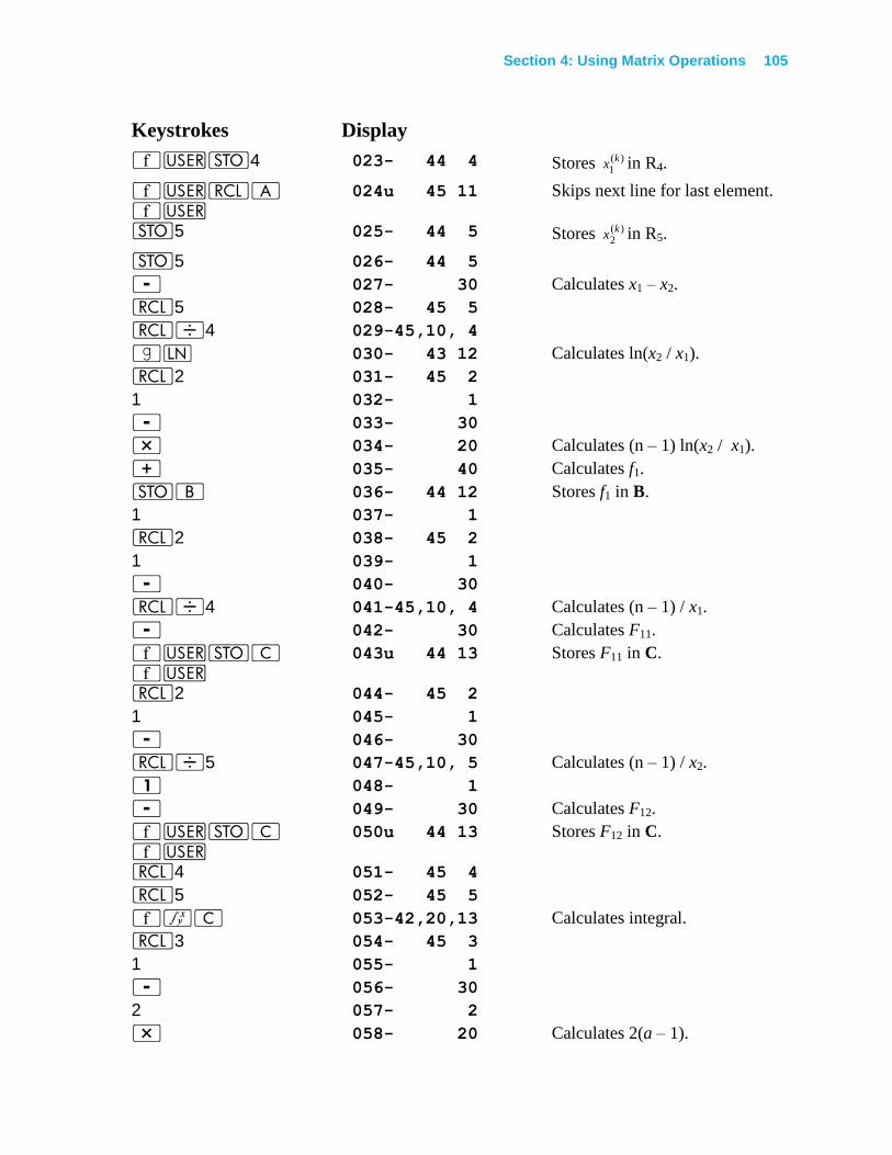
Section 4: Using Matrix Operations 105
Keystrokes Display
´UO4 023- 44 4 Stores )(1
kx in R4.
´UlA ´U
024u 45 11 Skips next line for last element.
O5 025- 44 5 Stores )(2k
x in R5.
O5 026- 44 5
- 027- 30 Calculates x1 – x2.
l5 028- 45 5
l÷4 029-45,10, 4
|N 030- 43 12 Calculates ln(x2 / x1).
l2 031- 45 2
1 032- 1
- 033- 30
* 034- 20 Calculates (n – 1) ln(x2 / x1).
+ 035- 40 Calculates f1.
OB 036- 44 12 Stores f1 in B.
1 037- 1
l2 038- 45 2
1 039- 1
- 040- 30
l÷4 041-45,10, 4 Calculates (n – 1) / x1.
- 042- 30 Calculates F11.
´UOC ´U
043u 44 13 Stores F11 in C.
l2 044- 45 2
1 045- 1
- 046- 30
l÷5 047-45,10, 5 Calculates (n – 1) / x2.
1 048- 1
- 049- 30 Calculates F12.
´UOC ´U
050u 44 13 Stores F12 in C.
l4 051- 45 4
l5 052- 45 5
´fC 053-42,20,13 Calculates integral.
l3 054- 45 3
1 055- 1
- 056- 30
2 057- 2
* 058- 20 Calculates 2(a – 1).
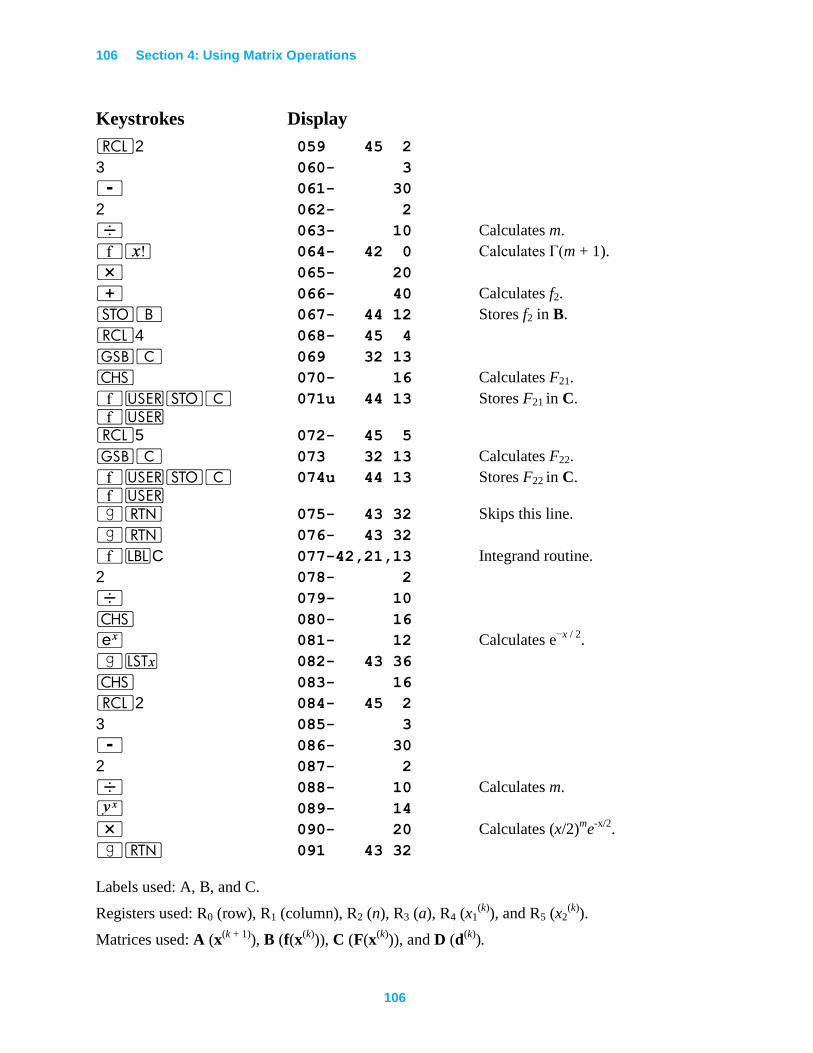
106 Section 4: Using Matrix Operations
106
Keystrokes Display
l2 059 45 2
3 060- 3
- 061- 30
2 062- 2
÷ 063- 10 Calculates m.
´! 064- 42 0 Calculates Γ(m + 1).
* 065- 20
+ 066- 40 Calculates f2.
OB 067- 44 12 Stores f2 in B.
l4 068- 45 4
GC 069 32 13
” 070- 16 Calculates F21.
´UOC ´U
071u 44 13 Stores F21 in C.
l5 072- 45 5
GC 073 32 13 Calculates F22.
´UOC ´U
074u 44 13 Stores F22 in C.
|n 075- 43 32 Skips this line.
|n 076- 43 32
´bC 077-42,21,13 Integrand routine.
2 078- 2
÷ 079- 10
” 080- 16
' 081- 12 Calculates e−x / 2
.
|K 082- 43 36
” 083- 16
l2 084- 45 2
3 085- 3
- 086- 30
2 087- 2
÷ 088- 10 Calculates m.
Y 089- 14
* 090- 20 Calculates (x/2)me
-x/2.
|n 091 43 32
Labels used: A, B, and C.
Registers used: R0 (row), R1 (column), R2 (n), R3 (a), R4 (x1(k)
), and R5 (x2(k)
).
Matrices used: A (x(k + 1)
), B (f(x(k)
)), C (F(x(k)
)), and D (d(k)
).
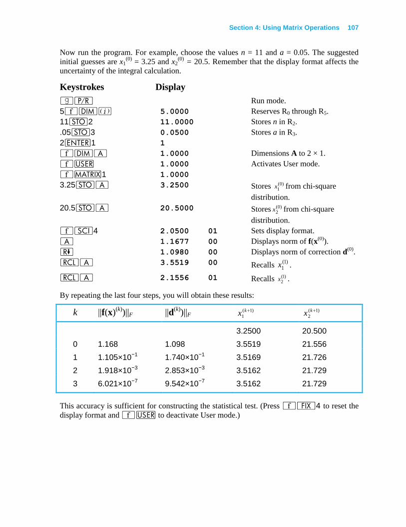
Section 4: Using Matrix Operations 107
Now run the program. For example, choose the values n = 11 and a = 0.05. The suggested
initial guesses are x1(0)
= 3.25 and x2(0)
= 20.5. Remember that the display format affects the
uncertainty of the integral calculation.
Keystrokes Display
|¥ Run mode.
5´m% 5.0000 Reserves R0 through R5.
11O2 11.0000 Stores n in R2.
.05O3 0.0500 Stores a in R3.
2v1 1
´mA 1.0000 Dimensions A to 2 × 1.
´U 1.0000 Activates User mode.
´>1 1.0000
3.25OA 3.2500 Stores )0(1
x from chi-square
distribution.
20.5OA 20.5000 Stores )0(2
x from chi-square
distribution.
´i4 2.0500 01 Sets display format.
A 1.1677 00 Displays norm of f(x(0)
).
) 1.0980 00 Displays norm of correction d(0)
.
lA 3.5519 00 Recalls )1(
1x .
lA 2.1556 01 Recalls )1(2
x .
By repeating the last four steps, you will obtain these results:
k ||f(x)(k)
)||F ||d(k)
)||F )1(
1
kx )1(
2
kx
3.2500 20.500
0 1.168 1.098 3.5519 21.556
1 1.105×10⁻¹ 1.740×10⁻¹ 3.5169 21.726
2 1.918×10⁻³ 2.853×10⁻³ 3.5162 21.729
3 6.021×10⁻⁷ 9.542×10⁻⁷ 3.5162 21.729
This accuracy is sufficient for constructing the statistical test. (Press ´•4 to reset the
display format and ´U to deactivate User mode.)
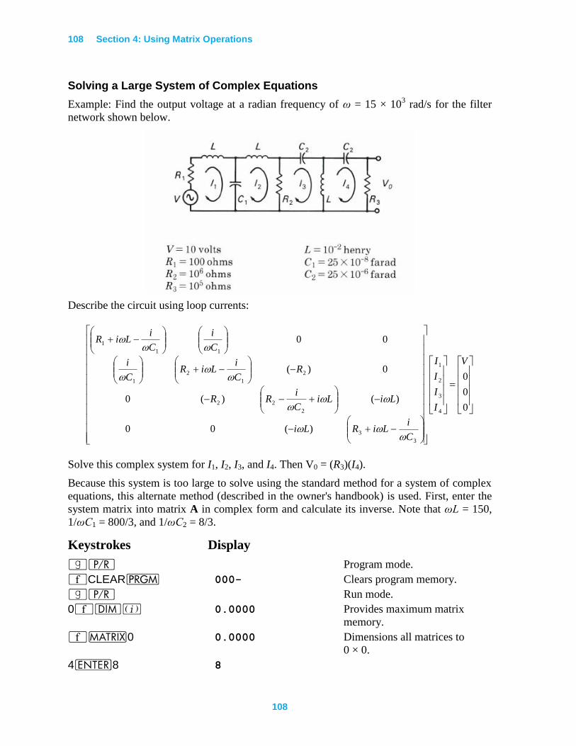
108 Section 4: Using Matrix Operations
108
Solving a Large System of Complex Equations
Example: Find the output voltage at a radian frequency of ω = 15 × 103 rad/s for the filter
network shown below.
Describe the circuit using loop currents:
0
0
0
)(00
)()(0
0)(
00
4
3
2
1
3
3
2
22
2
1
2
1
11
1
V
I
I
I
I
C
iLiRLi
LiLiC
iRR
RC
iLiR
C
i
C
i
C
iLiR
Solve this complex system for I1, I2, I3, and I4. Then V0 = (R3)(I4).
Because this system is too large to solve using the standard method for a system of complex
equations, this alternate method (described in the owner's handbook) is used. First, enter the
system matrix into matrix A in complex form and calculate its inverse. Note that ωL = 150,
1/ωC1 = 800/3, and 1/ωC2 = 8/3.
Keystrokes Display
|¥ Program mode.
´CLEARM 000- Clears program memory.
|¥ Run mode.
0´m% 0.0000 Provides maximum matrix
memory.
´>0 0.0000 Dimensions all matrices to
0 × 0.
4v8 8
Section 4: Using Matrix Operations 109
Keystrokes Display
´mA 8.0000 Dimensions matrix A to
4 × 8.
´>1 8.0000
´U 8.0000 Activates User mode.
100OA 100.0000 Stores Re(a11).
150v 150.0000
800v3÷ 266.6667
-OA -116.6667 Stores Im(a11).
⋮
150v 150.0000
8v3÷ 2.6667
-OA 147.3333 Stores Im(a44).
l>A A 4 8
´p A 8 4 Transforms AC to A
P.
´>2 A 8 8 Transforms AP to .
~A
O< A 8 8
´⁄ A 8 8 Calculates inverse of A~
in A.
Delete the second half of the rows of A to provide space to store the right-hand matrix B.
Keystrokes Display
4v8 8
´mA 8.0000 Redimensions matrix A to
4 × 8.
4v2 2
´mB 2.0000 Dimensions matrix B to
4 × 2.
´>1 2.0000
10OB 10.0000 Stores Re(V). (Other elements
are 0.)
l>A A 4 8
l>B b 4 2
´p b 8 1 Transforms BC to B
P.
´>2 b 8 2 Transforms BP to B
~.
´<C b 8 2
* C 4 2 Calculates solution in C.
´>4 C 2 4 Calculates transpose.
´>2 C 2 8 Transforms C to C~
.
110 Section 4: Using Matrix Operations
110
Keystrokes Display
1v8 8
´mC 8.0000 Redimensions matrix C to
1 × 8.
l< C 1 8
´>4 C 8 1 Calculates transpose.
|c C 4 2 Transforms CP to C
C.
Matrix C contains the desired values of I1, I2, I3, and I4 in rectangular form. Their phasor
forms are easy to compute:
Keystrokes Display
´>1 C 4 2 Resets R0 and R1.
´i4 C 4 2
lC 1.9550 -04 Recalls Re(I1).
lC 4.0964 -03 Recalls Im(I1).
®|: 4.1013 -03 Displays |I1|.
® 8.7212 01 Displays Arg(I1) in degrees.
lC -1.4489 -03
lC -3.5633 -02
®|: 3.5662 -02 Displays |I2|.
® -9.2328 01
lC -1.4541 -03
lC -3.5633 -02
®|: 3.5662 -02 Displays |I3|.
® -9.2337 01
lC 5.3446 -05
lC -2.2599 -06
®|: 5.3494 -05 Displays |I4|.
® -2.4212 00
®“5* 5.3494 00 Calculates |V0| = (R3)|I4|.
´•4 5.3494
´U 5.3494 Deactivates User mode.
The output voltage is 5.3494 ∠ −2.4212°.
Section 4: Using Matrix Operations 111
Least-Squares Using Normal Equations
The unconstrained least-squares problem is known in statistical literature as multiple linear
regression. It uses the linear model
p
j
jj rxby1
Here, b1, …, bp are the unknown parameters, xl, ..., xp are the independent (or explanatory)
variables, y is the dependent (or response) variable, and r is the random error having
expected value E(r) = 0, variance σ2.
After making n observations of y and x1, x2, ..., xp, this problem can be expressed as
y = Xb + r
where y is an n-vector, X is an n × p matrix, and r is an n-vector consisting of the unknown
random errors satisfying E(r) = 0 and Cov(r) = E(rrT) = σ
2In.
If the model is correct and XTX has an inverse, then the calculated least-squares solution
yXXXbTT 1)(ˆ has the following properties:
E( b̂ ) = b, so that b̂ is an unbiased estimator of b.
Cov( b̂ ) = E(( b̂ − b)T( b̂ − b)) = σ
2(X
TX)
–l, the covariance matrix of the estimator b̂ .
E( r̂ ) = 0, where r̂ = y − X b̂ is the vector of residuals.
22 )()||ˆ(||E pnF bXy , so that )/(||ˆ||ˆ 22 pnF r is an unbiased estimator for
σ2. You can estimate Cov( b̂ ) by replacing σ
2 by 2̂ .
The total sum of squares 2|||| Fy can be partitioned according to
2|||| Fy = y
Ty
= (y − X b̂ + X b̂ )T(y − X b̂ + X b̂ )
= (y − X b̂ )T(y − X b̂ ) - 2 b̂ T
XT(y − X b̂ ) + (X b̂ )
T(X b̂ )
= 22 ||ˆ||||ˆ|| FF bXbXy
=
SquaresofSum
Regression
SquaresofSum
Residual.
When the model is correct,
2222 ||||||ˆ||E pp FF XbbX
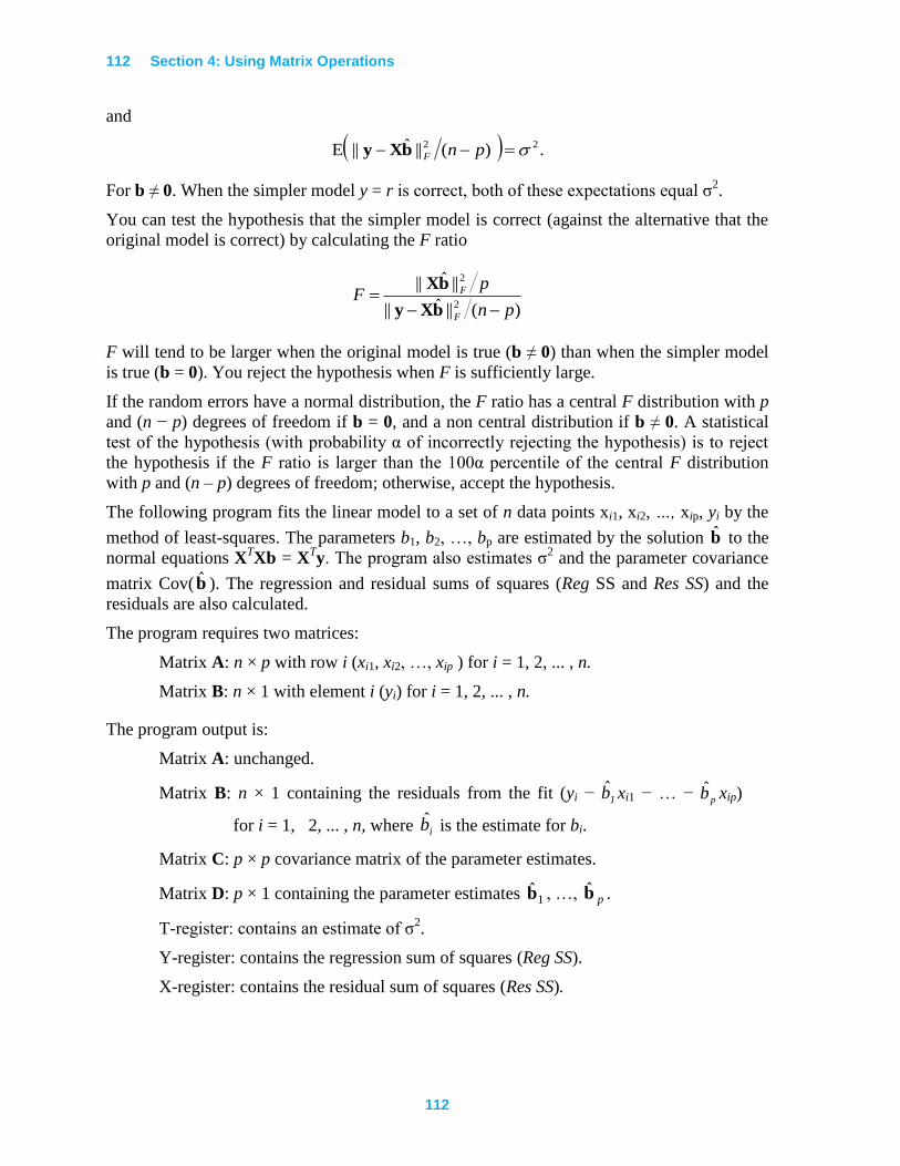
112 Section 4: Using Matrix Operations
112
and
.)(||ˆ||E 22 pnFbXy
For b ≠ 0. When the simpler model y = r is correct, both of these expectations equal σ2.
You can test the hypothesis that the simpler model is correct (against the alternative that the
original model is correct) by calculating the F ratio
)(||ˆ||
||ˆ||2
2
pn
pF
F
F
bXy
bX
F will tend to be larger when the original model is true (b ≠ 0) than when the simpler model
is true (b = 0). You reject the hypothesis when F is sufficiently large.
If the random errors have a normal distribution, the F ratio has a central F distribution with p
and (n − p) degrees of freedom if b = 0, and a non central distribution if b ≠ 0. A statistical
test of the hypothesis (with probability α of incorrectly rejecting the hypothesis) is to reject
the hypothesis if the F ratio is larger than the 100α percentile of the central F distribution
with p and (n – p) degrees of freedom; otherwise, accept the hypothesis.
The following program fits the linear model to a set of n data points xi1, xi2, …, xip, yi by the
method of least-squares. The parameters b1, b2, …, bp are estimated by the solution b̂ to the
normal equations XTXb = X
Ty. The program also estimates σ
2 and the parameter covariance
matrix Cov( b̂ ). The regression and residual sums of squares (Reg SS and Res SS) and the
residuals are also calculated.
The program requires two matrices:
Matrix A: n × p with row i (xi1, xi2, …, xip ) for i = 1, 2, ... , n.
Matrix B: n × 1 with element i (yi) for i = 1, 2, ... , n.
The program output is:
Matrix A: unchanged.
Matrix B: n × 1 containing the residuals from the fit (yi − 1b̂ xi1 − … − pb̂ xip)
for i = 1, 2, ... , n, where ib̂ is the estimate for bi.
Matrix C: p × p covariance matrix of the parameter estimates.
Matrix D: p × 1 containing the parameter estimates 1b̂ , …, pb̂ .
T-register: contains an estimate of σ2.
Y-register: contains the regression sum of squares (Reg SS).
X-register: contains the residual sum of squares (Res SS).
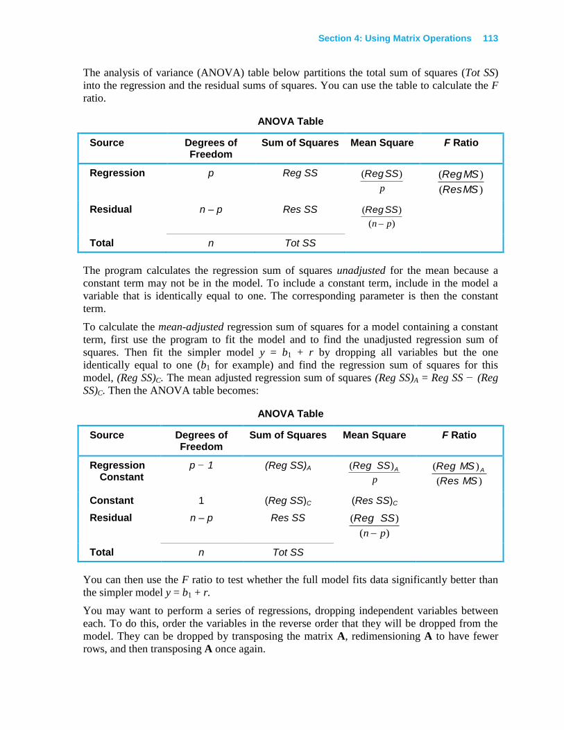
Section 4: Using Matrix Operations 113
The analysis of variance (ANOVA) table below partitions the total sum of squares (Tot SS)
into the regression and the residual sums of squares. You can use the table to calculate the F
ratio.
ANOVA Table
Source Degrees of Freedom
Sum of Squares Mean Square F Ratio
Regression p Reg SS
p
)( SSReg
)(
)(
MSRes
MSReg
Residual n – p
Res SS
)(
)(
pn
SSReg
Total n Tot SS
The program calculates the regression sum of squares unadjusted for the mean because a
constant term may not be in the model. To include a constant term, include in the model a
variable that is identically equal to one. The corresponding parameter is then the constant
term.
To calculate the mean-adjusted regression sum of squares for a model containing a constant
term, first use the program to fit the model and to find the unadjusted regression sum of
squares. Then fit the simpler model y = b1 + r by dropping all variables but the one
identically equal to one (b1 for example) and find the regression sum of squares for this
model, (Reg SS)C. The mean adjusted regression sum of squares (Reg SS)A = Reg SS − (Reg
SS)C. Then the ANOVA table becomes:
ANOVA Table
Source Degrees of Freedom
Sum of Squares Mean Square F Ratio
Regression Constant
p − 1 (Reg SS)A
p
ASSReg )(
)(
)(
MSRes
MSReg A
Constant 1 (Reg SS)C (Res SS)C
Residual n – p
Res SS
)(
)(
pn
SSReg
Total n Tot SS
You can then use the F ratio to test whether the full model fits data significantly better than
the simpler model y = b1 + r.
You may want to perform a series of regressions, dropping independent variables between
each. To do this, order the variables in the reverse order that they will be dropped from the
model. They can be dropped by transposing the matrix A, redimensioning A to have fewer
rows, and then transposing A once again.
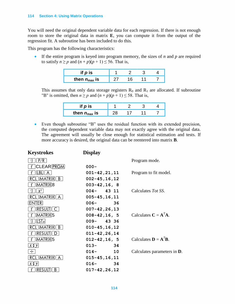
114 Section 4: Using Matrix Operations
114
You will need the original dependent variable data for each regression. If there is not enough
room to store the original data in matrix E, you can compute it from the output of the
regression fit. A subroutine has been included to do this.
This program has the following characteristics:
If the entire program is keyed into program memory, the sizes of n and p are required
to satisfy n ≥ p and (n + p)(p + 1) ≤ 56. That is,
if p is 1 2 3 4
then nmax is 27 16 11 7
This assumes that only data storage registers R0 and R1 are allocated. If subroutine
"B" is omitted, then n ≥ p and (n + p)(p + 1) ≤ 58. That is,
if p is 1 2 3 4
then nmax is 28 17 11 7
Even though subroutine “B” uses the residual function with its extended precision,
the computed dependent variable data may not exactly agree with the original data.
The agreement will usually be close enough for statistical estimation and tests. If
more accuracy is desired, the original data can be reentered into matrix B.
Keystrokes Display
|¥ Program mode.
´CLEARM 000-
´bA 001-42,21,11 Program to fit model.
l>B 002-45,16,12
´>8 003-42,16, 8
|x 004- 43 11 Calculates Tot SS.
l>A 005-45,16,11
v 006- 36
´<C 007-42,26,13
´>5 008-42,16, 5 Calculates C = ATA.
|K 009- 43 36
l>B 010-45,16,12
´<Á 011-42,26,14
´>5 012-42,16, 5 Calculates D = ATB.
® 013- 34
÷ 014- 10 Calculates parameters in D.
l>A 015-45,16,11
® 016- 34
´<B 017-42,26,12
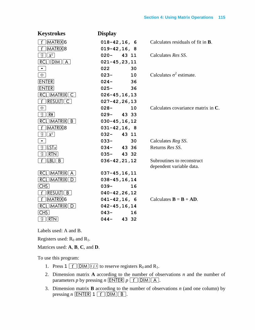
Section 4: Using Matrix Operations 115
Keystrokes Display
´>6 018-42,16, 6 Calculates residuals of fit in B.
´>8 019-42,16, 8
|x 020- 43 11 Calculates Res SS.
lmA 021-45,23,11
- 022 30
÷ 023- 10 Calculates σ2 estimate.
v 024- 36
v 025- 36
l>C 026-45,16,13
´<C 027-42,26,13
÷ 028- 10 Calculates covariance matrix in C.
|( 029- 43 33
l>B 030-45,16,12
´>8 031-42,16, 8
|x 032- 43 11
- 033- 30 Calculates Reg SS.
|K 034- 43 36 Returns Res SS.
|n 035- 43 32
´bB 036-42,21,12 Subroutines to reconstruct
dependent variable data.
l>A 037-45,16,11
l>Á 038-45,16,14
” 039- 16
´<B 040-42,26,12
´>6 041-42,16, 6 Calculates B = B + AD.
l>Á 042-45,16,14
” 043- 16
|n 044- 43 32
Labels used: A and B.
Registers used: R0 and R1.
Matrices used: A, B, C, and D.
To use this program:
1. Press 1 ´m% to reserve registers R0 and R1.
2. Dimension matrix A according to the number of observations n and the number of
parameters p by pressing n v p ´mA.
3. Dimension matrix B according to the number of observations n (and one column) by
pressing n v 1 ´mB.
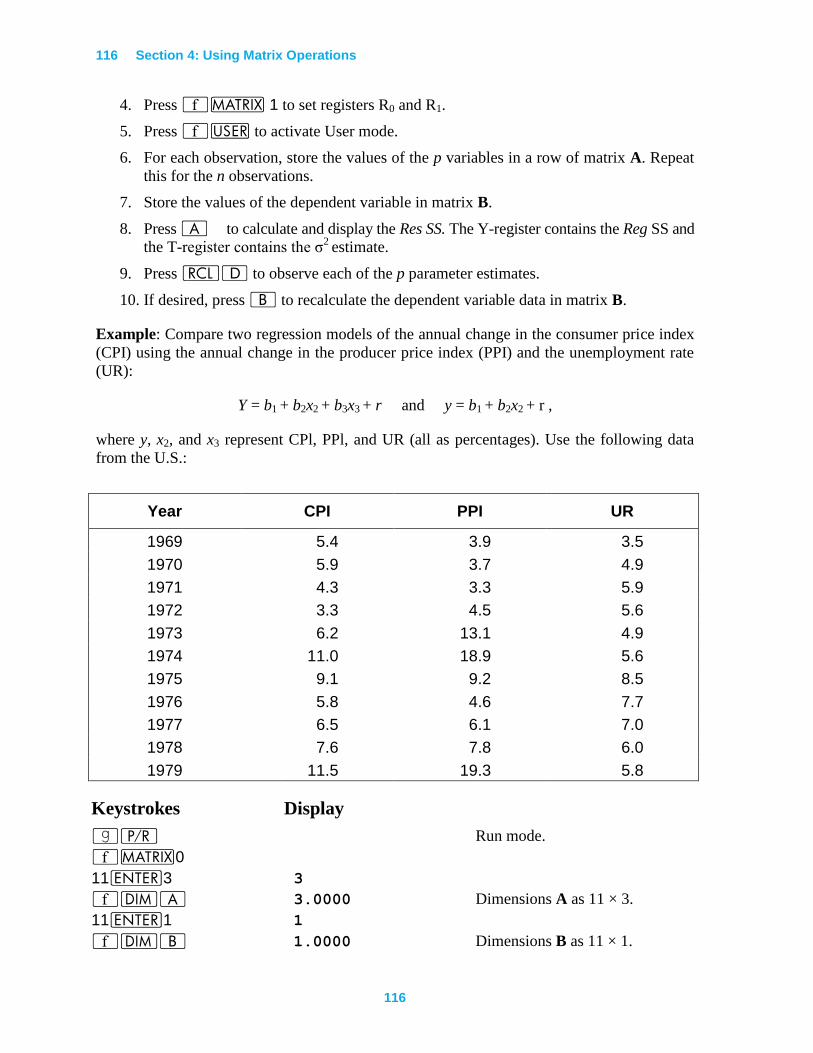
116 Section 4: Using Matrix Operations
116
4. Press ´> 1 to set registers R0 and R1.
5. Press ´U to activate User mode.
6. For each observation, store the values of the p variables in a row of matrix A. Repeat
this for the n observations.
7. Store the values of the dependent variable in matrix B.
8. Press A to calculate and display the Res SS. The Y-register contains the Reg SS and
the T-register contains the σ2
estimate.
9. Press lÁ to observe each of the p parameter estimates.
10. If desired, press B to recalculate the dependent variable data in matrix B.
Example: Compare two regression models of the annual change in the consumer price index
(CPI) using the annual change in the producer price index (PPI) and the unemployment rate
(UR):
Y = b1 + b2x2 + b3x3 + r and y = b1 + b2x2 + r ,
where y, x2, and x3 represent CPl, PPl, and UR (all as percentages). Use the following data
from the U.S.:
Year CPI PPI UR
1969 5.4 3.9 3.5
1970 5.9 3.7 4.9
1971 4.3 3.3 5.9
1972 3.3 4.5 5.6
1973 6.2 13.1 4.9
1974 11.0 18.9 5.6
1975 9.1 9.2 8.5
1976 5.8 4.6 7.7
1977 6.5 6.1 7.0
1978 7.6 7.8 6.0
1979 11.5 19.3 5.8
Keystrokes Display
|¥ Run mode.
´>0
11v3 3
´mA 3.0000 Dimensions A as 11 × 3.
11v1 1
´mB 1.0000 Dimensions B as 11 × 1.
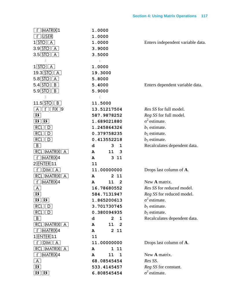
Section 4: Using Matrix Operations 117
´>1 1.0000
´U 1.0000
1OA 1.0000 Enters independent variable data.
3.9OA 3.9000
3.5OA 3.5000
⋮ ⋮
1OA 1.0000
19.3OA 19.3000
5.8OA 5.8000
5.4OB 5.4000 Enters dependent variable data.
5.9OB 5.9000
⋮ ⋮
11.5OB 11.5000
A´•9 13.51217504 Res SS for full model.
) 587.9878252 Reg SS for full model.
)) 1.689021880 σ2
estimate.
lÁ 1.245864326 b1 estimate.
lÁ 0.379758235 b2 estimate.
lÁ 0.413552218 b3 estimate.
B d 3 1 Recalculates dependent data.
l>A A 11 3
´>4 A 3 11
2v11 11
´mA 11.00000000 Drops last column of A.
l>A A 2 11
´>4 A 11 2 New A matrix.
A 16.78680552 Res SS for reduced model.
) 584.7131947 Reg SS for reduced model.
)) 1.865200613 σ2
estimate.
lÁ 3.701730745 b1 estimate.
lÁ 0.380094935 b2 estimate.
B d 2 1 Recalculates dependent data.
l>A A 11 2
´>4 A 2 11
1v11 11
´mA 11.00000000 Drops last column of A.
l>A A 1 11
´>4 A 11 1 New A matrix.
A 68.08545454 Res SS.
) 533.4145457 Reg SS for constant.
)) 6.808545454 σ2
estimate.
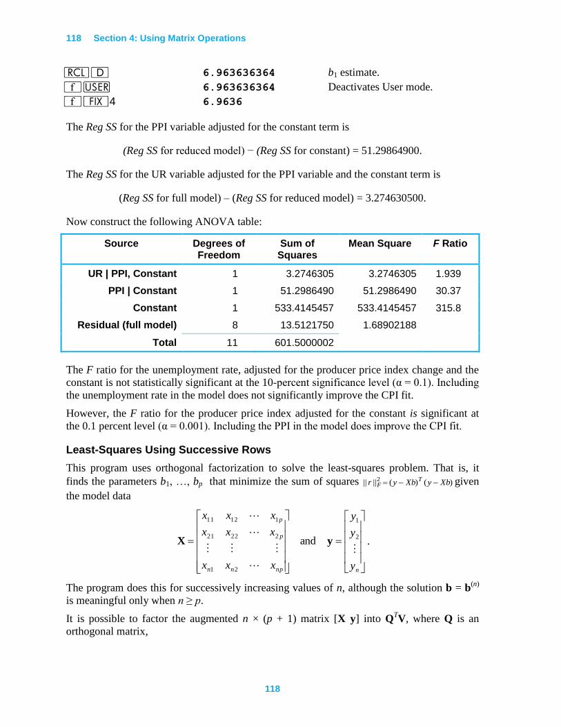
118 Section 4: Using Matrix Operations
118
lÁ 6.963636364 b1 estimate.
´U 6.963636364 Deactivates User mode.
´•4 6.9636
The Reg SS for the PPI variable adjusted for the constant term is
(Reg SS for reduced model) − (Reg SS for constant) = 51.29864900.
The Reg SS for the UR variable adjusted for the PPI variable and the constant term is
(Reg SS for full model) – (Reg SS for reduced model) = 3.274630500.
Now construct the following ANOVA table:
Source Degrees of Freedom
Sum of Squares
Mean Square F Ratio
UR | PPI, Constant 1 3.2746305 3.2746305 1.939
PPI | Constant 1 51.2986490 51.2986490 30.37
Constant 1 533.4145457 533.4145457 315.8
Residual (full model) 8 13.5121750 1.68902188
Total 11 601.5000002
The F ratio for the unemployment rate, adjusted for the producer price index change and the
constant is not statistically significant at the 10-percent significance level (α = 0.1). Including
the unemployment rate in the model does not significantly improve the CPI fit.
However, the F ratio for the producer price index adjusted for the constant is significant at
the 0.1 percent level (α = 0.001). Including the PPI in the model does improve the CPI fit.
Least-Squares Using Successive Rows
This program uses orthogonal factorization to solve the least-squares problem. That is, it
finds the parameters b1, …, bp that minimize the sum of squares )()(|||| 2 XbyXbyr TF given
the model data
nnpnn
p
p
y
y
y
xxx
xxx
xxx
2
1
21
22221
11211
and yX .
The program does this for successively increasing values of n, although the solution b = b(n)
is meaningful only when n ≥ p.
It is possible to factor the augmented n × (p + 1) matrix [X y] into QTV, where Q is an
orthogonal matrix,
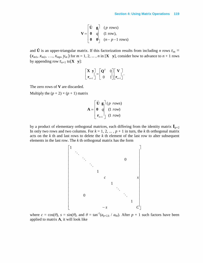
Section 4: Using Matrix Operations 119
)rows1(
),row1(
rows)(ˆ
pn
p
q
00
0
gU
V
and Û is an upper-triangular matrix. If this factorization results from including n rows rm =
(xm1, xm2, …, xmp, ym ) for m = 1, 2, ... , n in [X y], consider how to advance to n + 1 rows
by appending row rn+1 to[X y]:
11 10
0
n
T
n r
VQ
r
yX.
The zero rows of V are discarded.
Multiply the (p + 2) × (p + 1) matrix
)1(
)1(
)(ˆ
1 row
row
rowsp
q
n
r
0
gU
A
by a product of elementary orthogonal matrices, each differing from the identity matrix Ip+2 In only two rows and two columns. For k = 1, 2, ... , p + 1 in turn, the k th orthogonal matrix
acts on the k th and last rows to delete the k th element of the last row to alter subsequent
elements in the last row. The k th orthogonal matrix has the form
Cs
sc
1
0
1
1
0
1
where c = cos(θ), s = sin(θ), and θ = tan-1
(ap+2,k / akk). After p + 1 such factors have been
applied to matrix A, it will look like
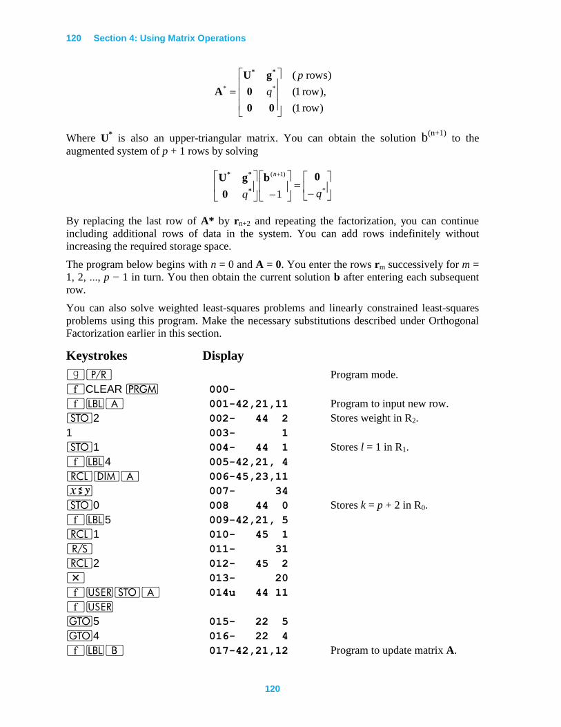
120 Section 4: Using Matrix Operations
120
)row1(
),row1(
rows)(*
p
q*
00
0
gU
A
**
Where U* is also an upper-triangular matrix. You can obtain the solution b
(n+1) to the
augmented system of p + 1 rows by solving
*
)1(
1 qq
n 0b
0
gU*
**
By replacing the last row of A* by rn+2 and repeating the factorization, you can continue
including additional rows of data in the system. You can add rows indefinitely without
increasing the required storage space.
The program below begins with n = 0 and A = 0. You enter the rows rm successively for m =
1, 2, ..., p − 1 in turn. You then obtain the current solution b after entering each subsequent
row.
You can also solve weighted least-squares problems and linearly constrained least-squares
problems using this program. Make the necessary substitutions described under Orthogonal
Factorization earlier in this section.
Keystrokes Display
|¥ Program mode.
´CLEAR M 000-
´bA 001-42,21,11 Program to input new row.
O2 002- 44 2 Stores weight in R2.
1 003- 1
O1 004- 44 1 Stores l = 1 in R1.
´b4 005-42,21, 4
lmA 006-45,23,11
® 007- 34
O0 008 44 0 Stores k = p + 2 in R0.
´b5 009-42,21, 5
l1 010- 45 1
¦ 011- 31
l2 012- 45 2
* 013- 20
´UOA 014u 44 11
´U
t5 015- 22 5
t4 016- 22 4
´bB 017-42,21,12 Program to update matrix A.
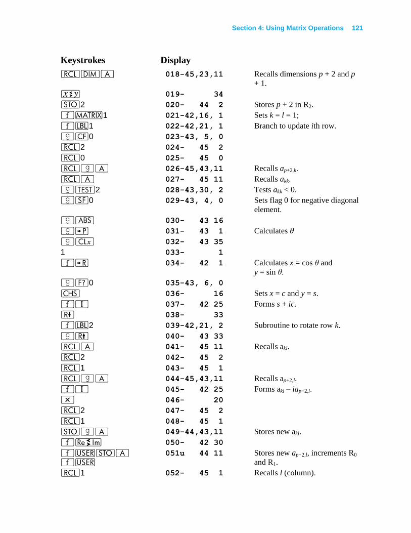
Section 4: Using Matrix Operations 121
Keystrokes Display
lmA 018-45,23,11 Recalls dimensions p + 2 and p
+ 1.
® 019- 34
O2 020- 44 2 Stores p + 2 in R2.
´>1 021-42,16, 1 Sets k = l = 1;
´b1 022-42,21, 1 Branch to update ith row.
|"0 023-43, 5, 0
l2 024- 45 2
l0 025- 45 0
l|A 026-45,43,11 Recalls ap+2,k.
lA 027- 45 11 Recalls akk.
|T2 028-43,30, 2 Tests akk < 0.
|F0 029-43, 4, 0 Sets flag 0 for negative diagonal
element.
|a 030- 43 16
|: 031- 43 1 Calculates θ
|` 032- 43 35
1 033- 1
´; 034- 42 1 Calculates x = cos θ and
y = sin θ.
|?0 035-43, 6, 0
” 036- 16 Sets x = c and y = s.
´V 037- 42 25 Forms s + ic.
) 038- 33
´b2 039-42,21, 2 Subroutine to rotate row k.
|( 040- 43 33
lA 041- 45 11 Recalls akl.
l2 042- 45 2
l1 043- 45 1
l|A 044-45,43,11 Recalls ap+2,l.
´V 045- 42 25 Forms akl – iap+2,l.
* 046- 20
l2 047- 45 2
l1 048- 45 1
O|A 049-44,43,11 Stores new akl.
´} 050- 42 30
´UOA ´U
051u 44 11 Stores new ap+2,l, increments R0
and R1.
l1 052- 45 1 Recalls l (column).
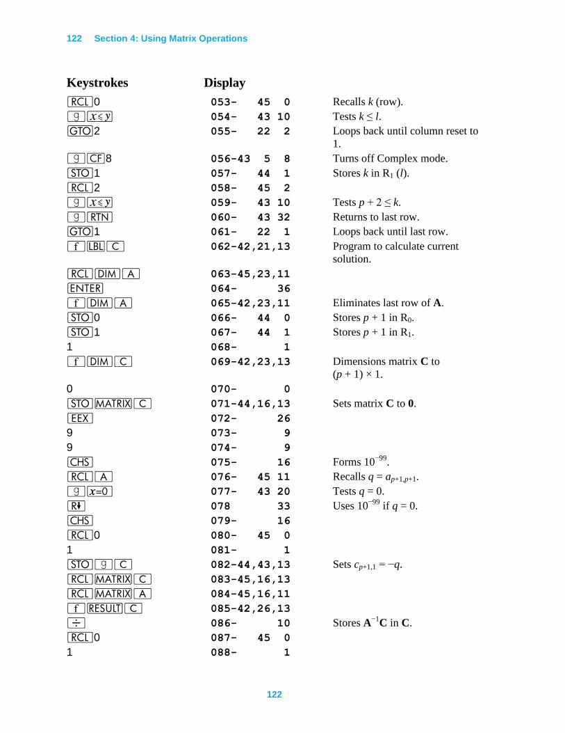
122 Section 4: Using Matrix Operations
122
Keystrokes Display
l0 053- 45 0 Recalls k (row).
|£ 054- 43 10 Tests k ≤ l.
t2 055- 22 2 Loops back until column reset to
1.
|"8 056-43 5 8 Turns off Complex mode.
O1 057- 44 1 Stores k in R1 (l).
l2 058- 45 2
|£ 059- 43 10 Tests p + 2 ≤ k.
|n 060- 43 32 Returns to last row.
t1 061- 22 1 Loops back until last row.
´bC 062-42,21,13 Program to calculate current
solution.
lmA 063-45,23,11
v 064- 36
´mA 065-42,23,11 Eliminates last row of A.
O0 066- 44 0 Stores p + 1 in R0.
O1 067- 44 1 Stores p + 1 in R1.
1 068- 1
´mC 069-42,23,13 Dimensions matrix C to
(p + 1) × 1.
0 070- 0
O>C 071-44,16,13 Sets matrix C to 0.
“ 072- 26
9 073- 9
9 074- 9
” 075- 16 Forms 10−99
.
lA 076- 45 11 Recalls q = ap+1,p+1.
|~ 077- 43 20 Tests q = 0.
) 078 33 Uses 10−99
if q = 0.
” 079- 16
l0 080- 45 0
1 081- 1
O|C 082-44,43,13 Sets cp+1,1 = −q.
l>C 083-45,16,13
l>A 084-45,16,11
´<C 085-42,26,13
÷ 086- 10 Stores A−1
C in C.
l0 087- 45 0
1 088- 1
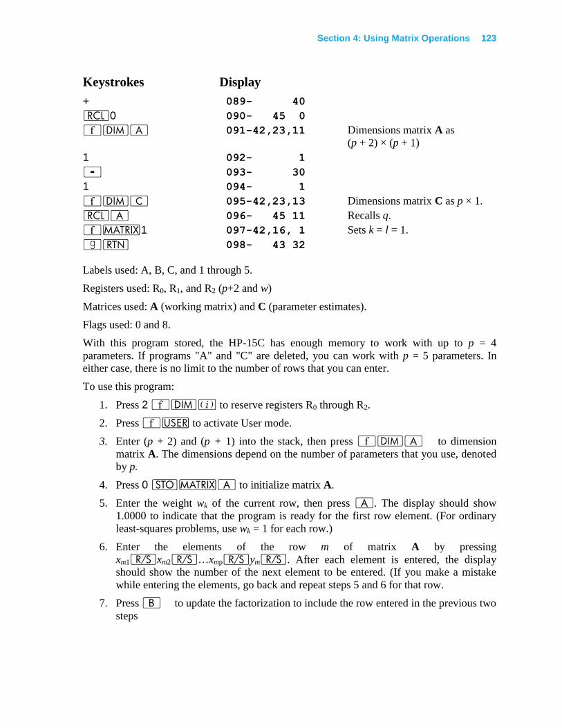
Section 4: Using Matrix Operations 123
Keystrokes Display
+ 089- 40
l0 090- 45 0
´mA 091-42,23,11 Dimensions matrix A as
(p + 2) × (p + 1)
1 092- 1
- 093- 30
1 094- 1
´mC 095-42,23,13 Dimensions matrix C as p × 1.
lA 096- 45 11 Recalls q.
´>1 097-42,16, 1 Sets k = l = 1.
|n 098- 43 32
Labels used: A, B, C, and 1 through 5.
Registers used: R0, R1, and R2 (p+2 and w)
Matrices used: A (working matrix) and C (parameter estimates).
Flags used: 0 and 8.
With this program stored, the HP-15C has enough memory to work with up to p = 4
parameters. If programs "A" and "C" are deleted, you can work with p = 5 parameters. In
either case, there is no limit to the number of rows that you can enter.
To use this program:
1. Press 2 ´m% to reserve registers R0 through R2.
2. Press ´U to activate User mode.
3. Enter (p + 2) and (p + 1) into the stack, then press ´mA to dimension
matrix A. The dimensions depend on the number of parameters that you use, denoted
by p.
4. Press 0 O>A to initialize matrix A.
5. Enter the weight wk of the current row, then press A. The display should show
1.0000 to indicate that the program is ready for the first row element. (For ordinary
least-squares problems, use wk = 1 for each row.)
6. Enter the elements of the row m of matrix A by pressing
xm1¦xm2¦…xmp¦ym¦. After each element is entered, the display
should show the number of the next element to be entered. (If you make a mistake
while entering the elements, go back and repeat steps 5 and 6 for that row.
7. Press B to update the factorization to include the row entered in the previous two
steps

124 Section 4: Using Matrix Operations
124
8. Optionally, press C|x to calculate and display the residual sum of squares q2
and to calculate the current solution b. Then press lCp times to display b1, b2,
…, bp in turn.
9. Repeat steps 5 through 8 for each additional row.
Example: Use this program and the CPI data from the previous example to fit the model
y = bl + b2x2 + b3x3 + r,
where y, x2, and x3 represent the CPI, PPI, and UR (all as percentages).
This problem involves p = 3 parameters, so matrix A should be 5 × 4. The rows of matrix A
are (1, xm2, xm3, ym) for m = 1,2, ... , 11. Each row has weight wm = 1.
Keystrokes Display
|¥ Run mode.
2´m% 2.0000 Reserves R0 through R2.
´U 2.0000 Activates User mode.
´>0 2.0000 Clears matrix memory.
5v4 4
´mA 4.0000 Dimensions matrix A to 5 ×4.
0O>A 0.0000 Stores zero in all elements.
1A 1.0000 Enters weight for row 1.
1¦ 2.0000 Enters x11.
3.9¦ 3.0000 Enters x12.
3.5¦ 4.0000 Enters x13.
5.4¦ 1.0000 Enters y1.
B 5.0000 Updates factorization.
⋮ ⋮
1A 1.0000 Enters weight for row 11.
1¦ 2.0000 Enters x11,1.
19.3¦ 3.0000 Enters x11,2.
5.8¦ 4.0000 Enters x11,3.
11.5¦ 1.0000 Enters y11.
B 5.0000 Updates factorization.
C 3.6759 Calculates current estimates and q.
´•9 3.675891055
|x 13.51217505 Calculates residual sum of squares
q2.
lC 1.245864306 Displays )11(1
b .
lC 0.379758235 Displays )11(2
b .
lC 0.413552221 Displays )11(3
b .
Section 4: Using Matrix Operations 125
These estimates agree (to within 3 in the ninth significant digit) with the results of the
preceding example, which uses the normal equations. In addition, you can include additional
data and update the parameter estimates. For example, add this data from 1968: CPI = 4.2,
PPI = 2.5 and UR = 3.6.
Keystrokes Display
1A 1.000000000 Enters row weight for new row.
1¦ 2.000000000 Enters x12,1.
2.5¦ 3.000000000 Enters x12,2.
3.6¦ 4.000000000 Enters x12,3.
4.2¦ 1.000000000 Enters y12.
B 1.000000000 Updates factorization.
C 3.700256908
|x 13.691900119 Calculates residual sum of
squares.
lC 1.581596327 Displays )12(1
b .
lC 0.373826487 Displays )12(2
b .
lC 0.370971848 Displays )12(3
b .
´•4 0.3710
´U 0.3710 Deactivates User mode.
Eigenvalues of a Symmetric Real Matrix
The eigenvalues of a square matrix A are the roots λj of its characteristic equation
det(A − λI) = 0.
When A is real and symmetric (A = AT) its eigenvalues λj are all real and possess orthogonal
eigenvectors qj. Then
Aqj= λjqj
and
.1
0
kjif
kjifk
T
j qq
The eigenvectors (q1, q2,…) constitute the columns of an orthogonal matrix Q which satisfies
QTAQ = diag(λ1, λ2, …)
and
QT = Q
−1.
126 Section 4: Using Matrix Operations
126
An orthogonal change of variables x = Qz, which is equivalent to rotating the coordinate
axes, changes the equation of a family of quadratic surfaces (xTAx = constant) into the form
.constantλ)( 2 k
j
jj
TTzzAQQz
With the equation in this form, you can recognize what kind of surfaces these are (ellipsoids,
hyperboloids, paraboloids, cones, cylinders, planes) because the surface's semi-axes lie along
the new coordinate axes.
The program below starts with a given matrix A that is assumed to be symmetric (if it isn't, it
is replaced by (A + AT)/2, which is symmetric).
Given a symmetric matrix A, the program constructs a skew-symmetric matrix (that is, one
for which B = −BT) using the formula
.00
0)))/(2(tan¼tan( -1
ij
ijjjiiij
ijaorjiif
aandjiifaaab
Then Q = 2(I + B)−1
− I must be an orthogonal matrix whose columns approximate the
eigenvalues of A; the smaller are all the elements of B, the better the approximation.
Therefore QTAQ must be more nearly diagonal than A but with the same eigenvalues. If
QTAQ is not close enough to diagonal, it is used in place of A above for a repetition of the
process.
In this way, successive orthogonal transformations Q1, Q2, Q3, ... are applied to A to produce
a sequence A1, A2, A3, ... , where
Aj = (Q1 Q2… Qj)TAQ1Q2…Qj
with each successive Aj more nearly diagonal than the one before.
This process normally leads to skew matrices whose elements are all small and Aj rapidly
converging to a diagonal matrix A. However, if some of the eigenvalues of matrix A are very
close but far from the others, convergence is slow; fortunately, this situation is rare.
The program stops after each iteration to display
jFj
j
A
A |ofelementsdiagonaloff|
2
1
which measures how nearly diagonal is Aj. If this measure is not negligible, you can press
¦ to calculate Aj+1; if it is negligible, then the diagonal elements of Aj approximate the
eigenvalues of A. The program needs only one iteration for 1 × 1 and 2 × 2 matrices, and
rarely more than six for 3 × 3 matrices. For 4 × 4 matrices the program takes slightly longer
and uses all available memory; usually 6 or 7 iterations are sufficient, but if some
eigenvalues are very close to each other and relatively far from the rest, then 10 to 16
iterations may be needed.
Section 4: Using Matrix Operations 127
Keystrokes Display
|¥ Program mode.
´CLEARM 000
´bA 001-42,21,11
l>A 002-45,16,11
O>B 003-44,16,12 Dimensions B.
O>C 004-44,16,13 Dimensions C.
´>4 005-42,16, 4 Transposes A.
l>B 006-45,16,12
O< 007- 44 26
+ 008- 40
2 009- 2
÷ 010- 10
O>A 011-44,16,11 Calculates A = (A + AT)/2
´>8 012-42,16, 8 Calculates ||A||F.
O2 013- 44 2 Stores ||A||F in R2.
|` 014- 43 35
O3 015- 44 3 Initializes off-diagonal sum.
O>C 016-44,16,13 Sets C = 0.
´>1 017-42,16, 1 Sets R0 = R1 = 1.
´b0 018-42,21, 0 Routine to construct Q.
l0 019- 45 0
l1 020- 45 1
|T5 021-43,30, 5 Tests column = row.
t3 022- 22 3
|T7 023-43,30, 7 Tests column > row
t1 024- 22 1
® 025- 34
l|B 026-45,43,12
” 027- 16
´UOB 028u 44 12 Sets bij = −bji.
´U
t0 029- 22 0
´b1 030-42,21, 1 Routine for column > row.
l|A 031-43,43,11
|a 032- 43 16 Calculates |aij|.
O+3 033-44,40, 3 Accumulates off-diagonal sum.
|K 034- 43 36
v 035- 36
+ 036- 40 Calculates 2aij.
128 Section 4: Using Matrix Operations
128
Keystrokes Display
l0 037- 45 0
v 038- 36
l|A 039-45,43,11 Recalls aii.
l1 040- 45 1
v 041- 36
l|A 042-45,43,11 Recalls ajj.
- 043- 30 Calculates aii −ajj.
|T3 044-43,30, 3 Tests x ≥ 0.
t2 045- 22 2
” 046- 16 Keeps angle of rotation between
−90° and 90°.
® 047- 34
” 048- 16
® 049- 34
´b2 050-42,21, 2
|: 051- 43 1 Calculates angle of rotation.
|` 052- 43 35
4 053- 4
÷ 054- 10
] 055- 25 Calculates bij.
´UOB 056u 44 12
´U
t0 057- 22 0
´b3 058-42,21, 3 Routine for row = column.
1 059- 1
OC 060- 44 13 Sets cii = 1.
´UOB 061u 44 12 Sets bii = 1.
´U
t0 062- 22 0
l3 063- 45 3
l÷2 064-45,10, 2 Calculates off-diagonal ratio.
¦ 065- 31 Displays ratio.
2 066- 2
l>B 067-45,16,12
÷ 068- 10
l>C 069-45,16,13
- 070- 30 Calculates B = 2(I + skew)−1
– I.
l>A 071-45,16,11
´<C 072-42,26,13
Section 4: Using Matrix Operations 129
Keystrokes Display
´>5 073-42,16, 5 Calculates C = BTA.
l>B 074-45,16,12
´<A 075-42,26,11
* 076- 20 Calculates A = BTAB.
tA 077- 22 11
Labels used: A, 0, 1, 2, and 3.
Registers used: R0, R1, R2 (off-diagonal sum), and R3 (||Aj||F).
Matrices used: A (Aj), B (Qj), and C.
To use the program:
1. Press 4 ´m% to reserve registers R0 through R4.
2. Press ´U to activate User mode.
3. Dimension and enter the elements of matrix A using ´mA and OA.
The dimensions can be up to 4 × 4, provided that there is sufficient memory available
for matrices B and C having the same dimensions also.
4. Press A to calculate and display the off-diagonal ratio.
5. Press ¦ repeatedly until the displayed ratio is negligible, say less than 10−8
.
6. Press lA repeatedly to observe the elements of matrix A. The diagonal
elements are the eigenvalues.
Example: What quadratic surface is described by the equation below?
3
2
1
321
432
321
210
x
x
x
xxxTAxx
= 221 xx + 4
31 xx + 22
2x + 632 xx + 4
3
3x
= 7
Keystrokes Display
|¥ Run mode.
4´m% 4.0000 Allocates memory.
´U 4.0000 Activates User mode.
3v´mA 3.0000 Dimensions A to 3 × 3.
´>1 3.0000 Sets R0 and R1 to 1.
0OA 0.0000 Enters a11.
1OA 1.0000 Enters a12.
130 Section 4: Using Matrix Operations
130
Keystrokes Display
⋮
3OA 3.0000 Enters a32.
4OA 4.0000 Enters a33.
A 0.8660 Calculates ratio-too large.
¦ 0.2304 Again, too large.
¦ 0.1039 Again, too large.
¦ 0.0060 Again, too large.
¦ 3.0463 -05 Again, too large.
¦ 5.8257 -10 Negligible ratio.
lA -0.8730 Recalls a11=λ1.
lA -9.0006 -10 Recalls a12.
lA -2.0637 -09 Recalls a13.
lA -9.0006 -10 Recalls a21.
lA 9.3429 -11 Recalls a22=λ2.
lA 1.0725 -09 Recalls a23.
lA -2.0637 -09 Recalls a31.
lA 1.0725 -09 Recalls a32.
lA 6.8730 Recalls a33=λ3.
´U 6.8730 Deactivates User mode.
In the new coordinate system the equation of the quadratic surface is approximately
−0.87302
1z + 02
2z + 6.87302
3z = 7
This is the equation of a hyperbolic cylinder.
Eigenvectors of a Symmetric Real Matrix
As discussed in the previous application, a real symmetric matrix A has real eigenvalues λ1,
λ2 ... and corresponding orthogonal eigenvectors ql, q2, ... .
This program uses inverse iteration to calculate an eigenvector qk that corresponds to the
eigenvalue λk such that ||qk||R = 1. The technique uses an initial vector z(0)
to calculate
subsequent vectors w(n)
and z(n)
repeatedly from the equations
)()1( nnzwIA
R
nnn s )1()1()1( wwz
where s denotes the sign of the first component of w(n+1)
having the largest absolute value.
The iterations continue until z(n)
converges. That vector is an eigenvector qk corresponding to
the eigenvalue λk.
Section 4: Using Matrix Operations 131
The value used for λk need not be exact; the calculated eigenvector is determined accurately
in spite of small inaccuracies in λk. Furthermore, don't be concerned about having too
accurate an approximation to λk; the HP-15C can calculate the eigenvector even when
A − λk I is very ill-conditioned.
This technique requires that vector z(0)
have a nonzero component along the unknown
eigenvector qk.. Because there are no other restrictions on z(0)
, the program uses random
components for z(0)
. At the end of each iteration, the program displays ||z(n+1) − z
(n)||R to show
the rate of convergence.
This program can accommodate a matrix A that isn't symmetric but has a diagonal Jordan
canonical form−that is, there exists some nonsingular matrix P such that P-1
AP= diag(λ1, λ2,
…).
Keystrokes Display
|¥ Program mode.
´CLEARM 000-
´bC 001-42,21,13
O2 002- 44 2 Stores eigenvalue in R2
l>A 003-45,16,11
O>B 004-44,16,12 Stores A in B.
lmA 005-45,23,11
O0 006- 44 0
´b4 007-42,21, 4
l0 008- 45 0
O1 009- 44 1
lB 010- 45 12
l-2 011-45,30, 2
OB 012- 44 12 Modifies diagonal elements of
B.
´e0 013-42, 5, 0
t4 014- 22 4
lmA 015-45,23,11
1 016- 1
´mC 017-42,23,13 Dimensions C to n × 1.
´>1 018-42,16, 1
´b5 019-42,21, 5
´# 020- 42 36
´UOC´U
021u 44 13 Stores random components in
C.
t5 022- 22 5
´b6 023-42,21, 6 Routine for iterating z(n)
and
w(n)
.
132 Section 4: Using Matrix Operations
132
Keystrokes Display
l>C 024-45,16,13
O>Á 025-44,16,14 Stores z(n)
in D.
O< 026- 44 26
l>B 027-45,16,12
÷ 028- 10 Calculates w(n+1)
in C.
v 029- 36
´>7 030-42,16, 7
÷ 031- 10 Calculates ±z(n+1)
in C.
´>1 032-42,16, 1
´b7 033-42,21, 7 Routine to find sign of largest
element.
´UlC ´U
034u 45 13
v 035- 36 (This line skipped for last
element.)
|a 036- 43 16
1 037- 1
|T6 038-43,30, 6 Tests |aj|≠1
t7 039- 22 7
l>C 040-45,16,13
|K 041- 43 36 Recalls extreme aj.
÷ 042- 10 Calculates z(n+1)
in C.
l>Á 043-45,16,14
O< 044- 44 26
- 045- 30 Calculates z(n+1)-z
(n) in D.
´>7 046-42,16, 7 Calculates ||z(n+1)-z
(n)||R.
´>1 047-42,16, 1 Sets R0=R1=1 for viewing C.
¦ 048- 31 Displays convergence
parameter.
t6 049- 22 6
Labels used: C, 4, 5, 6, and 7.
Registers used: R0, R1, and R2 (eigenvalue).
Matrices used: A (original matrix), B (A − λI), C (z(n+1)
), and D (z(n+1)
− z(n)
).
To use this program:
1. Press 2 ´m% to reserve registers R0, R1, and R2.
2. Press ´U to activate User mode.
Section 4: Using Matrix Operations 133
3. Dimension and enter the elements into matrix A using ´mA, ´>1,
and OA.
4. Key in the eigenvalue and press C. The display shows the correction parameter
||z(1) − z
(0)||R.
5. Press ¦ repeatedly until the correction parameter is negligibly small.
6. Press lC repeatedly to view the components of qk, the eigenvector.
Example: For matrix A of the previous example,
432
321
210
A
Calculate the eigenvectors q1, q2, and q3.
Keystrokes Display
|¥ Run mode.
2´m% 2.0000 Reserves registers R0 through
R2.
´U 2.0000 Activates User mode.
3v´mA 3.0000 Dimensions A to 3 × 3.
´>1 3.0000
0OA 0.0000 Enters elements of A
1OA 1.0000
⋮
4OA 4.0000
.8730” -0.8730 Enters λ1=−0.8730
(approximation).
C 0.8982 ||z(1) − z(0)
||.*
¦ 0.0001 ||z
(2) − z(1)||.*
¦ 2.4000 -09 ||z
(3) − z(2)||.*
¦ 1.0000 -10 ||z
(4) − z(3)||.*
¦ 0.0000 ||z
(5) − z(4)||.*
lC 1.0000
lC 0.2254 Eigenvector forλ1.
lC -0.5492
0C 0.8485 Uses λ2=0 (approximation).
¦ 0.0000
* The correction norms will vary, depending upon the current random number seed.
134 Section 4: Using Matrix Operations
134
Keystrokes Display
lC -0.5000
lC 1.0000 Eigenvector forλ2.
lC -0.5000
6.8730C 0.7371 Uses λ3=6.8730
(approximation).
¦ 1.9372 -06
¦ 1.0000 -10
¦ 0.0000
lC 0.3923
lC 0.6961 Eigenvector forλ3.
lC 1.0000
´U 1.0000 Deactivates User mode.
If matrix A is no larger than 3×3, this program can be included with the previous eigenvalue
program. Since the eigenvalue program modifies matrix A, the original eigenvalues must be
saved and the original matrix reentered in matrix A before running the eigenvector program.
The following program can be added to store the calculated eigenvalues in matrix E.
Keystrokes Display
´bE 127-42,21,15
lmA 128-45,23,11
O0 129- 44 0
1 130- 1
´mE 131-42,23,15 Dimensions E to n × 1.
´b8 132-42,21, 8
l0 133- 45 0
v 134- 36
l|A 135-45,43,11 Recalls diagonal element.
l0 136- 45 0
1 137- 1
O|E 138-44,43,15 Stores aii in ei.
´e0 139-42, 5, 0
t8 140- 22 8
´>1 141-42,16, 1 Resets R0=R1=1.
|n 142- 43 32
|¥ Run mode.
Section 4: Using Matrix Operations 135
Labels used: E and 8.
Registers used: no additional registers.
Matrices used: A (from previous program) and E (eigenvalues).
To use the combined eigenvalue, eigenvalue storage, and eigenvector programs for an A
matrix up to 3×3:
1. Execute the eigenvalue program as described earlier.
2. Press E to store the eigenvalues.
3. Enter again the elements of the original matrix into A.
4. Recall the desired eigenvalue from matrix E using l E.
5. Execute the eigenvector program as described above.
6. Repeat steps 4 and 5 for each eigenvalue.
Optimization
Optimization describes a class of problems in which the object is to find the minimum or
maximum value of a specified function. Often, the interest is focused on the behavior of the
function in a particular region.
The following program uses the method of steepest descent to determine local minimums or
maximums for a real-valued function of two or more variables. This method is an iterative
procedure that uses the gradient of the function to determine successive sample points. Four
input parameters control the sampling plan.
For the function
f (x) = f (x1,x2, … ,xn)
the gradient of f, f, is defined by
n
2
1
)(
xf
xf
xf
f
x
The critical points of f(x) are the solutions to f (x) = 0. A critical point may be a local
minimum, a local maximum, or a point that is neither.
The gradient of f(x) evaluated at a point x gives the direction of steepest ascent—that is, the
way in which x should be changed in order to cause the most rapid increase in f(x). The
negative gradient gives the direction of steepest descent. The direction vector is
136 Section 4: Using Matrix Operations
136
maximum.afindingfor)(
minimumafindingfor)(
x
xs
f
f
Once the direction is determined from the gradient, the program looks for the optimum
distance to move from xj in the direction indicated by sj—the distance that gives the greatest
improvement in f(x) toward a minimum or maximum
To do this, the program finds the optimum value tj by calculating the slope of the function
gj(t) = f(xj + tsj)
at increasing values of t until the slope changes sign. This procedure is called "bounding
search" since the program tries to bound the desired value tj within an interval. When the
program finds a change of sign, it then reduces the interval by halving it j + 1 times to find
the best t value near t=0. This procedure is called "interval reduction"—it yields more
accurate values for tj as xj converges toward the desired solution. (These two processes are
collectively called "line search.") The new value of x is then
xj+1 = xj + tjsj.
The program uses four parameters that define how it proceeds toward the desired solution.
Although no method of line search can guarantee success for finding an optimum value of t,
the first two parameters give you considerable flexibility in specifying how the program
samples t.
d Determines the initial step u1 for the bounding search. The first value of t tried is
Fjj
du
s)1(1
.
This corresponds to a distance of
1
1
j
du
Fjjj xsx ,
which shows that d and the iteration number define how close to the last x value the
program starts the bounding search.
a Determines the values u2, u3, … of subsequent steps in the bounding search. These
values of t are defined by
ui+1 = aui
Essentially, a is an expansion factor that is normally greater than 1, producing an
increasing sequence of values of t.
e Determines the acceptable tolerance on the size of the gradient. The iterative process
stops when
||f(xj)||F e.
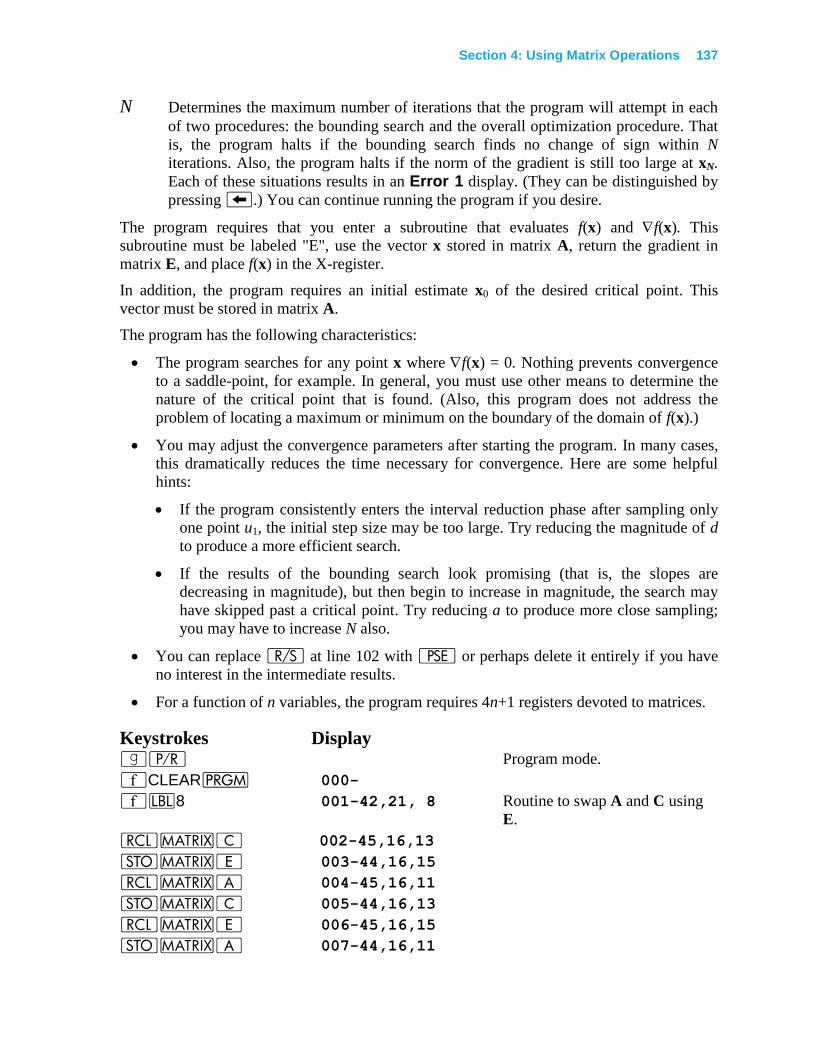
Section 4: Using Matrix Operations 137
N Determines the maximum number of iterations that the program will attempt in each
of two procedures: the bounding search and the overall optimization procedure. That
is, the program halts if the bounding search finds no change of sign within N
iterations. Also, the program halts if the norm of the gradient is still too large at xN.
Each of these situations results in an Error 1 display. (They can be distinguished by
pressing −.) You can continue running the program if you desire.
The program requires that you enter a subroutine that evaluates f(x) and f(x). This
subroutine must be labeled "E", use the vector x stored in matrix A, return the gradient in
matrix E, and place f(x) in the X-register.
In addition, the program requires an initial estimate x0 of the desired critical point. This
vector must be stored in matrix A.
The program has the following characteristics:
The program searches for any point x where f(x) = 0. Nothing prevents convergence
to a saddle-point, for example. In general, you must use other means to determine the
nature of the critical point that is found. (Also, this program does not address the
problem of locating a maximum or minimum on the boundary of the domain of f(x).)
You may adjust the convergence parameters after starting the program. In many cases,
this dramatically reduces the time necessary for convergence. Here are some helpful
hints:
If the program consistently enters the interval reduction phase after sampling only
one point u1, the initial step size may be too large. Try reducing the magnitude of d
to produce a more efficient search.
If the results of the bounding search look promising (that is, the slopes are
decreasing in magnitude), but then begin to increase in magnitude, the search may
have skipped past a critical point. Try reducing a to produce more close sampling;
you may have to increase N also.
You can replace ¦ at line 102 with © or perhaps delete it entirely if you have
no interest in the intermediate results.
For a function of n variables, the program requires 4n+1 registers devoted to matrices.
Keystrokes Display
|¥ Program mode.
´CLEARM 000-
´b8 001-42,21, 8 Routine to swap A and C using
E.
l>C 002-45,16,13
O>E 003-44,16,15
l>A 004-45,16,11
O>C 005-44,16,13
l>E 006-45,16,15
O>A 007-44,16,11
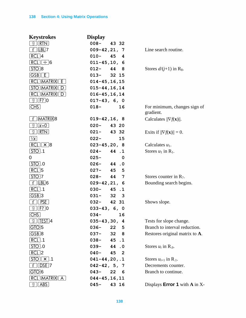
138 Section 4: Using Matrix Operations
138
Keystrokes Display
|n 008- 43 32
´b7 009-42,21, 7 Line search routine.
l4 010- 45 4
l÷6 011-45,10, 6
O8 012- 44 8 Stores d/(j+1) in R8.
GE 013- 32 15
l>E 014-45,16,15
O>Á 015-44,16,14
l>Á 016-45,16,14
|?0 017-43, 6, 0
” 018- 16 For minimum, changes sign of
gradient.
´>8 019-42,16, 8 Calculates ||f(x)||.
|~ 020- 43 20
|n 021- 43 32 Exits if ||f(x)|| = 0.
⁄ 022- 15
l*8 023-45,20, 8 Calculates u1.
O.1 024- 44 .1 Stores u1 in R1.
0 025- 0
O.0 026- 44 .0
l5 027- 45 5
O7 028- 44 7 Stores counter in R7.
´b6 029-42,21, 6 Bounding search begins.
l.1 030- 45 .1
G3 031- 32 3
´© 032- 42 31 Shows slope.
|?0 033-43, 6, 0
” 034- 16
|T4 035-43,30, 4 Tests for slope change.
t5 036- 22 5 Branch to interval reduction.
G8 037- 32 8 Restores original matrix to A.
l.1 038- 45 .1
O.0 039- 44 .0 Stores ui in R.0.
l2 040- 45 2
O*.1 041-44,20,.1 Stores ui+1 in R.1.
´s7 042-42, 5, 7 Decrements counter.
t6 043- 22 6 Branch to continue.
l>A 044-45,16,11
|a 045- 43 16 Displays Error 1 with A in X-
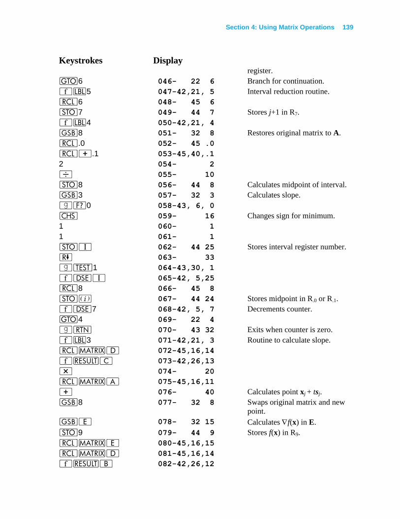
Section 4: Using Matrix Operations 139
Keystrokes Display
register.
t6 046- 22 6 Branch for continuation.
´b5 047-42,21, 5 Interval reduction routine.
l6 048- 45 6
O7 049- 44 7 Stores j+1 in R7.
´b4 050-42,21, 4
G8 051- 32 8 Restores original matrix to A.
l.0 052- 45 .0
l+.1 053-45,40,.1
2 054- 2
÷ 055- 10
O8 056- 44 8 Calculates midpoint of interval.
G3 057- 32 3 Calculates slope.
|?0 058-43, 6, 0
” 059- 16 Changes sign for minimum.
1 060- 1
1 061- 1
OV 062- 44 25 Stores interval register number.
) 063- 33
|T1 064-43,30, 1
´eV 065-42, 5,25
l8 066- 45 8
O% 067- 44 24 Stores midpoint in R.0 or R.1.
´e7 068-42, 5, 7 Decrements counter.
t4 069- 22 4
|n 070- 43 32 Exits when counter is zero.
´b3 071-42,21, 3 Routine to calculate slope.
l>Á 072-45,16,14
´<C 073-42,26,13
* 074- 20
l>A 075-45,16,11
+ 076- 40 Calculates point xj + tsj.
G8 077- 32 8 Swaps original matrix and new
point.
GE 078- 32 15 Calculates f(x) in E.
O9 079- 44 9 Stores f(x) in R9.
l>E 080-45,16,15
l>Á 081-45,16,14
´<B 082-42,26,12
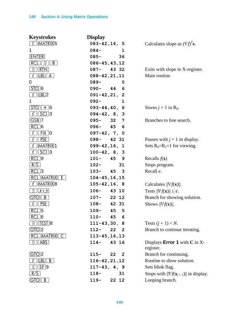
140 Section 4: Using Matrix Operations
140
Keystrokes Display
´>5 083-42,16, 5 Calculates slope as (f)Ts.
1 084- 1
v 085- 36
l|B 086-45,43,12
|n 087- 43 32 Exits with slope in X-register.
´bA 088-42,21,11 Main routine.
0 089- 0
O6 090- 44 6
´b2 091-42,21, 2
1 092- 1
O+6 093-44,40, 6 Stores j + 1 in R6.
´i3 094-42, 8, 3
G7 095- 32 7 Branches to line search.
l6 096- 45 6
´•0 097-42, 7, 0
´© 098- 42 31 Pauses with j + 1 in display.
´>1 099-42,16, 1 Sets R0=R1=1 for viewing.
´i3 100-42, 8, 3
l9 101- 45 9 Recalls f(x)
¦ 102- 31 Stops program.
l3 103- 45 3 Recall e.
l>E 104-45,16,15
´>8 105-42,16, 8 Calculates ||f(x)||.
|£ 106- 43 10 Tests ||f(x)|| ≤ e.
tB 107- 22 12 Branch for showing solution.
´© 108- 42 31 Shows ||f(x)||.
l5 109- 45 5
l6 110- 45 6
|T8 111-43,30, 8 Tests (j + 1) < N.
t2 112- 22 2 Branch to continue iterating.
l>C 113-45,16,13
|a 114- 43 16 Displays Error 1 with C in X-
register.
t2 115- 22 2 Branch for continuing.
´bB 116-42,21,12 Routine to show solution.
|F9 117-43, 4, 9 Sets blink flag.
¦ 118- 31 Stops with ||f(xj + 1)|| in display.
tB 119- 22 12 Looping branch.
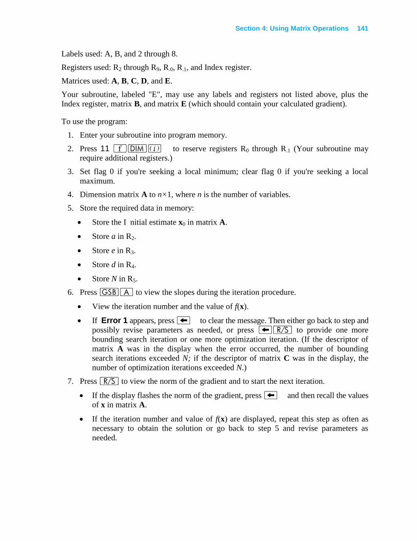
Section 4: Using Matrix Operations 141
Labels used: A, B, and 2 through 8.
Registers used: R2 through R9, R.0, R.1, and Index register.
Matrices used: A, B, C, D, and E.
Your subroutine, labeled "E", may use any labels and registers not listed above, plus the
Index register, matrix B, and matrix E (which should contain your calculated gradient).
To use the program:
1. Enter your subroutine into program memory.
2. Press 11 ´m% to reserve registers R0 through R.1 (Your subroutine may
require additional registers.)
3. Set flag 0 if you're seeking a local minimum; clear flag 0 if you're seeking a local
maximum.
4. Dimension matrix A to n×1, where n is the number of variables.
5. Store the required data in memory:
Store the I nitial estimate x0 in matrix A.
Store a in R2.
Store e in R3.
Store d in R4.
Store N in R5.
6. Press GA to view the slopes during the iteration procedure.
View the iteration number and the value of f(x).
If Error 1 appears, press − to clear the message. Then either go back to step and
possibly revise parameters as needed, or press −¦ to provide one more
bounding search iteration or one more optimization iteration. (If the descriptor of
matrix A was in the display when the error occurred, the number of bounding
search iterations exceeded N; if the descriptor of matrix C was in the display, the
number of optimization iterations exceeded N.)
7. Press ¦ to view the norm of the gradient and to start the next iteration.
If the display flashes the norm of the gradient, press − and then recall the values
of x in matrix A.
If the iteration number and value of f(x) are displayed, repeat this step as often as
necessary to obtain the solution or go back to step 5 and revise parameters as
needed.
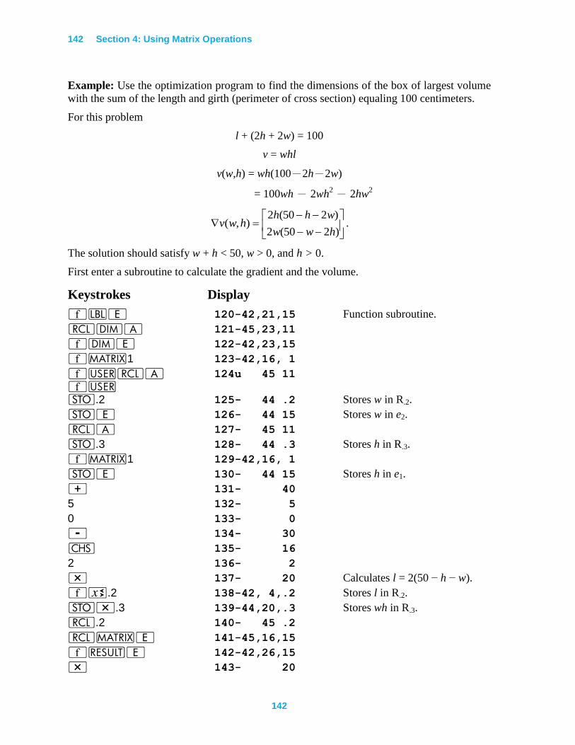
142 Section 4: Using Matrix Operations
142
Example: Use the optimization program to find the dimensions of the box of largest volume
with the sum of the length and girth (perimeter of cross section) equaling 100 centimeters.
For this problem
l + (2h + 2w) = 100
v = whl
v(w,h) = wh(100-2h-2w)
= 100wh - 2wh2 - 2hw
2
)250(2
)250(2),(
hww
whhhwv .
The solution should satisfy w + h < 50, w > 0, and h > 0.
First enter a subroutine to calculate the gradient and the volume.
Keystrokes Display
´bE 120-42,21,15 Function subroutine.
lmA 121-45,23,11
´mE 122-42,23,15
´>1 123-42,16, 1
´UlA ´U
124u 45 11
O.2 125- 44 .2 Stores w in R.2.
OE 126- 44 15 Stores w in e2.
lA 127- 45 11
O.3 128- 44 .3 Stores h in R.3.
´>1 129-42,16, 1
OE 130- 44 15 Stores h in e1.
+ 131- 40
5 132- 5
0 133- 0
- 134- 30
” 135- 16
2 136- 2
* 137- 20 Calculates l = 2(50 − h − w).
´X.2 138-42, 4,.2 Stores l in R.2.
O*.3 139-44,20,.3 Stores wh in R.3.
l.2 140- 45 .2
l>E 141-45,16,15
´<E 142-42,26,15
* 143- 20
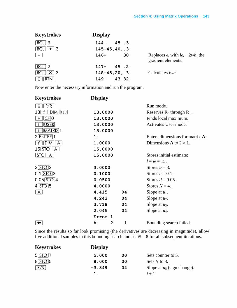
Section 4: Using Matrix Operations 143
Keystrokes Display
l.3 144- 45 .3
l+.3 145-45,40,.3
- 146- 30 Replaces ei with lei − 2wh, the
gradient elements.
l.2 147- 45 .2
l*.3 148-45,20,.3 Calculates lwh.
|n 149- 43 32
Now enter the necessary information and run the program.
Keystrokes Display
|¥ Run mode.
13´m% 13.0000 Reserves R0 through R.3.
|"0 13.0000 Finds local maximum.
´U 13.0000 Activates User mode.
´>1 13.0000
2v1 1 Enters dimensions for matrix A.
´mA 1.0000 Dimensions A to 2 × 1.
15OA 15.0000
OA 15.0000 Stores initial estimate:
l = w = 15.
3O2 3.0000 Stores a = 3.
0.1O3 0.1000 Stores e = 0.1 .
0.05O4 0.0500 Stores d = 0.05 .
4O5 4.0000 Stores N = 4.
A 4.415 04 Slope at u1.
4.243 04 Slope at u2.
3.718 04 Slope at u3.
2.045 04 Slope at u4.
Error 1
− A 2 1 Bounding search failed.
Since the results so far look promising (the derivatives are decreasing in magnitude), allow
five additional samples in this bounding search and set N = 8 for all subsequent iterations.
Keystrokes Display
5O7 5.000 00 Sets counter to 5.
8O5 8.000 00 Sets N to 8.
¦ -3.849 04 Slope at u5 (sign change).
1. j + 1.
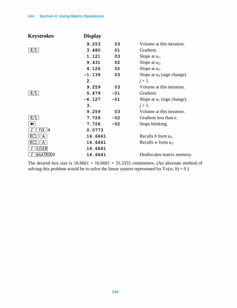
144 Section 4: Using Matrix Operations
144
Keystrokes Display
9.253 03 Volume at this iteration.
¦ 3.480 01 Gradient.
1.121 03 Slope at u1.
9.431 02 Slope at u2.
4.126 02 Slope at u3.
-1.139 03 Slope at u4 (sign change).
2. j + 1.
9.259 03 Volume at this iteration.
¦ 5.479 -01 Gradient.
-6.127 -01 Slope at u1 (sign change).
3. j + 1.
9.259 03 Volume at this iteration.
¦ 7.726 -02 Gradient less than e.
− 7.726 -02 Stops blinking.
´•4 0.0773
lA 16.6661 Recalls h form a1.
lA 16.6661 Recalls w form a2.
´U 16.6661
´>0 16.6661 Deallocates matrix memory.
The desired box size is 16.6661 × 16.6661 × 33.3355 centimeters. (An alternate method of
solving this problem would be to solve the linear system represented by v(w, h) = 0.)
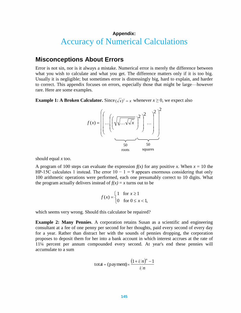
145
Appendix: Accuracy of Numerical Calculations
Misconceptions About Errors
Error is not sin, nor is it always a mistake. Numerical error is merely the difference between
what you wish to calculate and what you get. The difference matters only if it is too big.
Usually it is negligible; but sometimes error is distressingly big, hard to explain, and harder
to correct. This appendix focuses on errors, especially those that might be large—however
rare. Here are some examples.
Example 1: A Broken Calculator. Since xx 2)( whenever x ≥ 0, we expect also
22
22
)(
xxf
should equal x too.
A program of 100 steps can evaluate the expression f(x) for any positive x. When x = 10 the
HP-15C calculates 1 instead. The error 10 − 1 = 9 appears enormous considering that only
100 arithmetic operations were performed, each one presumably correct to 10 digits. What
the program actually delivers instead of f(x) = x turns out to be
,10for0
1for1)(
x
xxf
which seems very wrong. Should this calculator be repaired?
Example 2: Many Pennies. A corporation retains Susan as a scientific and engineering
consultant at a fee of one penny per second for her thoughts, paid every second of every day
for a year. Rather than distract her with the sounds of pennies dropping, the corporation
proposes to deposit them for her into a bank account in which interest accrues at the rate of
11¼ percent per annum compounded every second. At year's end these pennies will
accumulate to a sum
ni
nin
11)payment(total
50
roots
50
squares
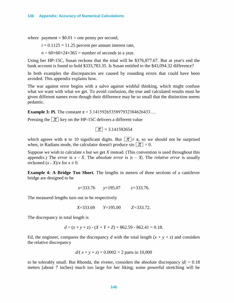
146 Appendix: Accuracy of Numerical Calculations
146
where payment = $0.01 = one penny per second,
i = 0.1125 = 11.25 percent per annum interest rate,
n = 60×60×24×365 = number of seconds in a year.
Using her HP-15C, Susan reckons that the total will be $376,877.67. But at year's end the
bank account is found to hold $333,783.35. Is Susan entitled to the $43,094.32 difference?
In both examples the discrepancies are caused by rounding errors that could have been
avoided. This appendix explains how.
The war against error begins with a salvo against wishful thinking, which might confuse
what we want with what we get. To avoid confusion, the true and calculated results must be
given different names even though their difference may be so small that the distinction seems
pedantic.
Example 3: Pi. The constant π = 3.1415926535897932384626433….
Pressing the $ key on the HP-15C delivers a different value
$ = 3.141592654
which agrees with π to 10 significant digits. But $≠ π, so we should not be surprised
when, in Radians mode, the calculator doesn't produce sin $ = 0.
Suppose we wish to calculate x but we get X instead. (This convention is used throughout this
appendix.) The error is x - X. The absolute error is |x – X|. The relative error is usually
reckoned (x - X)/x for x ≠ 0.
Example 4: A Bridge Too Short. The lengths in meters of three sections of a cantilever
bridge are designed to be
x=333.76 y=195.07 z=333.76.
The measured lengths turn out to be respectively
X=333.69 Y=195.00 Z=333.72.
The discrepancy in total length is
d = (x + y + z) - (X + Y + Z) = 862.59 - 862.41 = 0.18.
Ed, the engineer, compares the discrepancy d with the total length (x + y + z) and considers
the relative discrepancy
d/( x + y + z) = 0.0002 = 2 parts in 10,000
to be tolerably small. But Rhonda, the riveter, considers the absolute discrepancy |d| = 0.18
meters (about 7 inches) much too large for her liking; some powerful stretching will be
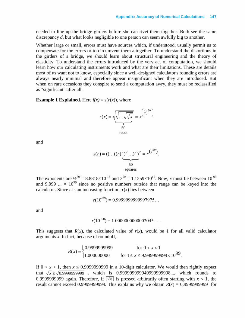
Appendix: Accuracy of Numerical Calculations 147
needed to line up the bridge girders before she can rivet them together. Both see the same
discrepancy d, but what looks negligible to one person can seem awfully big to another.
Whether large or small, errors must have sources which, if understood, usually permit us to
compensate for the errors or to circumvent them altogether. To understand the distortions in
the girders of a bridge, we should learn about structural engineering and the theory of
elasticity. To understand the errors introduced by the very act of computation, we should
learn how our calculating instruments work and what are their limitations. These are details
most of us want not to know, especially since a well-designed calculator's rounding errors are
always nearly minimal and therefore appear insignificant when they are introduced. But
when on rare occasions they conspire to send a computation awry, they must be reclassified
as "significant" after all.
Example 1 Explained. Here f(x) = s(r(x)), where
50
21
)( xxxr
and
.)(
))))(((()(50
22222 rrrs
The exponents are ½50
= 8.8818×10⁻¹⁶
and 250
= 1.1259×10¹⁵
. Now, x must lie between 10-99
and 9.999 ... × 1099
since no positive numbers outside that range can be keyed into the
calculator. Since r is an increasing function, r(x) lies between
r(10-99
) = 0.9999999999997975…
and
r(10100
) = 1.0000000000002045… .
This suggests that R(x), the calculated value of r(x), would be 1 for all valid calculator
arguments x. In fact, because of roundoff,
.9910999999999.91for000000000.1
10for9999999999.0)(
x
xxR
If 0 < x < 1, then x ≤ 0.9999999999 in a 10-digit calculator. We would then rightly expect
that 9999999999.0x , which is 0.999999999949999999998..., which rounds to
0.9999999999 again. Therefore, if ¤ is pressed arbitrarily often starting with x < 1, the
result cannot exceed 0.9999999999. This explains why we obtain R(x) = 0.9999999999 for
50
roots
50
squares
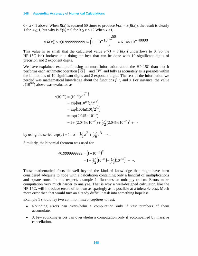
148 Appendix: Accuracy of Numerical Calculations
148
0 < x < 1 above. When R(x) is squared 50 times to produce F(x) = S(R(x)), the result is clearly
1 for x ≥ 1, but why is F(x) = 0 for 0 ≤ x < 1? When x <1,
.488981014.6
502101019999999999.0
sxRs
This value is so small that the calculated value F(x) = S(R(x)) underflows to 0. So the
HP-15C isn't broken; it is doing the best that can be done with 10 significant digits of
precision and 2 exponent digits.
We have explained example 1 using no more information about the HP-15C than that it
performs each arithmetic operation ¤ and x and fully as accurately as is possible within
the limitations of 10 significant digits and 2 exponent digits. The rest of the information we
needed was mathematical knowledge about the functions f, r, and s. For instance, the value
r(10100
) above was evaluated as
21313
13
50
50100
21
100100
)10045.2(2
1)10045.2(1
)10045.2exp(
2)10ln(100exp
2)10ln(exp
)10()10(
50
r
by using the series .36
122
11)exp( zzzz
Similarly, the binomial theorem was used for
.21010
21
10
108
1102
11
1019999999999.0
These mathematical facts lie well beyond the kind of knowledge that might have been
considered adequate to cope with a calculation containing only a handful of multiplications
and square roots. In this respect, example 1 illustrates an unhappy truism: Errors make
computation very much harder to analyze. That is why a well-designed calculator, like the
HP-15C, will introduce errors of its own as sparingly as is possible at a tolerable cost. Much
more error than that would turn an already difficult task into something hopeless.
Example 1 should lay two common misconceptions to rest:
Rounding errors can overwhelm a computation only if vast numbers of them
accumulate.
A few rounding errors can overwhelm a computation only if accompanied by massive
cancellation.
Appendix: Accuracy of Numerical Calculations 149
Regarding the first misconception, example 1 would behave in the same perverse way if it
suffered only one rounding error, the one that produces R(x) = 1 or 0.9999999999, in error by
less than one unit in its last (10th) significant digit.
Regarding the second misconception, cancellation is what happens when two nearly equal
numbers are subtracted. For example, calculating
2/)cos1()( xxxc
in Radians mode for small values of x is hazardous because of cancellation. Using x =
1.2×10⁻⁵
and rounding results to 10 digits
cos x = 0.9999999999
and
1 - cos x = 0.0000000001
with cancellation leaving maybe one significant digit in the numerator. Also
x2 = 1.44×10
-10.
Then
C(x) = 0.6944.
This calculated value is wrong because 2
1)(0 xc for all x≠ 0. To avoid numerical
cancellation, exploit the trigonometric identity 2sin21cos 2 xx to cancel the 1 exactly and
obtain a better formula
.
sin
2
1)(
2
2
2
x
xxc
When this latter expression is evaluated (in Radians mode) at x = 1.2×10⁻⁵
, the computed
result C(x) = 0.5 is correct to 10 significant digits. This example, while explaining the
meaning of the word "cancellation," suggests that it is always a bad thing. That is another
misconception to be dispatched later. For the present, recall that example 1 contains no
subtraction, therefore no cancellation, and is still devastated by its rounding error. In this
respect example 1 is counterintuitive, a little bit scary. Nowhere in it can we find one or two
arithmetic operations to blame for the catastrophe; no small rearrangement will set
everything right as happened for c(x). Alas, example 1 is not an isolated example. As
computers and calculators grow in power, so do instances of insidious error growth become
more common.
To help you recognize error growth and cope with it is the ultimate goal of this appendix. We
shall start with the simplest kinds of errors and work our way up gradually to the subtle
errors that can afflict the sophisticated computations possible on the HP-15C.
150 Appendix: Accuracy of Numerical Calculations
150
A Hierarchy of Errors
Some errors are easier to explain and to tolerate than others. Therefore, the functions
delivered by single keystrokes on the HP-15C have been categorized, for the purposes of
easier exposition, according to how difficult their errors are to estimate. The estimates should
be regarded as goals set by the calculator's designers rather than as specifications that
guarantee some stated level of accuracy. On the other hand, the designers believe they can
prove mathematically that their accuracy goals have been achieved, and extensive testing has
produced no indication so far that they might be mistaken.
Level 0: No Error
Functions which should map small integers (smaller than 1010
) to small integers do so
exactly, without error, as you might expect.
Examples:
24 -23
= -8 320
= 3,486,784,401
log(109) = 9 6! = 720
cos-1
(0) = 90 (in Degrees mode)
ABS(4,686,660 + 4,684,659 i) = 6,625,109 (in Complex mode)
Also exact for real arguments are a, q, ‘, &, and comparisons (such as
£). But the matrix functions *, ÷, ⁄, >6, and >9 (determinant)
are exceptions (refer to page 160).
Level ∞: Overflow/Underflow
Results which would lie closer to zero than 10-99
underflow quietly to zero. Any result that
would lie beyond the overflow thresholds ±9.999999999×1099
is replaced by the nearest
threshold, and then flag 9 is set and the display blinks. (Pressing == or "9 or −
will clear flag 9 and stop the blinking.) Most functions that result in more than one
component can tolerate overflow/underflow in one component without contaminating the
other; examples are ;, :, complex arithmetic, and most matrix operations. The
exceptions are matrix inversion (⁄ and ÷), > 9 (determinant), and L.
Level 1: Correctly Rounded, or Nearly So
Operations that deliver "correctly rounded" results whose error cannot exceed ½ unit in their
last (10th) significant digit include the real algebraic operations +, -, *, ÷, x,
¤, ⁄, and k, the complex and matrix operations + and -, matrix by scalar
operations *and ÷(excluding division by a matrix), and h. These results are the
best that 10 significant digits can represent, as are familiar constants $, 1', 2N,
10N, 1r, and many more. Operations that can suffer a slightly larger error, but still
Appendix: Accuracy of Numerical Calculations 151
significantly smaller than one unit in the 10th significant digit of the result, include ∆, À,r,d,p,and c; N,o, @,P]for real arguments;
:, ,, {, /,H[, H\and H]for real and complex
arguments; a, ¤, and⁄for complex arguments; matrix norms >7, >8;
and finally [, \, and ] for real arguments in Degrees and Grads modes (but not
in Radians mode − refer to Level 2, page 154)
A function that grows to ∞ or decays to 0 exponentially fast as its argument approaches ± ∞
may suffer an error larger than one unit in its 10th significant digit, but only if its magnitude
is smaller than 10-20
or larger than 1020
; and though the relative error gets worse as the result
gets more extreme (small or large), the error stays below three units in the last (10th)
significant digit. The reason for this error is explained later. Functions so affected, are ',
Y, ! (for non-integer x), P[, and P\ for real arguments. The worst
case known is 3201
, which calculated as 7.968419664×1095
. The last digit 4 should be 6
instead, as is the case for 7.2933.5
, calculated as 7.968419666×1028
.
The foregoing statements about errors can be summarized for all functions in Level 1 in a
way that will prove convenient later:
Attempts to calculate a function f in Level 1 produce instead a computed value F = (1 +ε) f
whose relative errorε, though unknown, is very small:
.1Levelinfunctionsotherallfor101
roundedcorrectlyif1059
10
F
F
This simple characterization of all the functions in Level l fails to convey many other
important properties they all possess, properties like
Exact integer values: mentioned in Level 0.
Sign symmetry: sinh(−x) = −sinh(x), cosh(−x) = cosh(x), ln(1/x) = −ln(x) (if l/x is
computed exactly).
Monotonicity: if f(x) ≥ f(y), then computed F(x) ≥ F(y).
These additional properties have powerful implications; for instance, TAN(20°) =
TAN(200°) = TAN(2,000°) = ... = TAN(2× 1099
°) = 0.3639702343 correctly. But the simple
characterization conveys most of what is worth knowing, and that can be worth money.
Example 2 Explained. Susan tried to calculate
ni
nin
11paymenttotal
where
payment = $0.01,
i = 0.1125, and
n = 60 × 60 × 24 × 365 = 31,536,000.
152 Appendix: Accuracy of Numerical Calculations
152
She calculated $376,877.67 on her HP-15C, but the bank's total was $333,783.35, and this
latter total agrees with the results calculated on good, modern financial calculators like the
HP-12C, HP-37E, HP-38E/38C, and HP-92. Where did Susan's calculation go awry? No
severe cancellation, no vast accumulation of errors; just one rounding error that grew
insidiously caused the damage:
i/n = 0.000000003567351598
1 + i/n = 1.000000004
when rounded to 10 significant digits. There is the rounding error that hurts. Subsequently
attempting to calculate (1+i/n)n, Susan must get instead (1.000000004)
31,536,000 =
1.134445516, which is wrong in its second decimal place.
How can the correct value be calculated? Only by not throwing away so many digits of i/n.
Observe that
nin
enni1ln
1 ,
so we might try to calculate the logarithm in some way that does not discard those precious
digits. An easy way to do so on the HP-15C does exist.
To calculate λ(x) = ln(1+x) accurately for all x>−1, even if |x| is very small:
1. Calculate u = 1 + x rounded.
2. Then
.11)ln(
1)(
uifuxu
uifxx
The following program calculates λ(x) = ln(1+x)
Keystrokes Display
|¥
´CLEARM 000-
´bA 001-42,21,11 Assumes x is in X-register.
v 002- 36
v 003- 36
“ 004- 26 Places 1 in X-register.
+ 005- 40 Calculates u = 1 + x rounded.
|N 006- 43 12 Calculates ln(u) (zero for u = 1).
® 007- 34 Restores x to X-register.
|K 008- 43 36 Recalls u.
“ 009- 26 Places 1 in X-register.
|T6 010-43,30, 6 Tests u≠1.
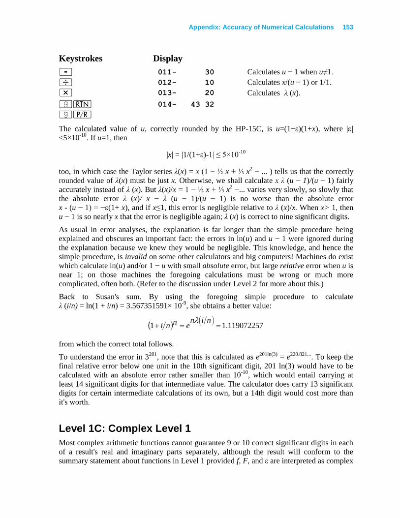
Appendix: Accuracy of Numerical Calculations 153
Keystrokes Display
- 011- 30 Calculates u − 1 when u≠1.
÷ 012- 10 Calculates x/(u − 1) or 1/1.
* 013- 20 Calculates λ(x).
|n 014- 43 32
|¥
The calculated value of u, correctly rounded by the HP-15C, is u=(1+ε)(1+x), where |ε|
<5×10⁻¹⁰
. If u=1, then
|x| = |1/(1+ε)-1| ≤ 5×10⁻¹⁰
too, in which case the Taylor series λ(x) = x (1 − ½ x + ⅓ x2 − ... ) tells us that the correctly
rounded value of λ(x) must be just x. Otherwise, we shall calculate x λ (u − 1)/(u − 1) fairly
accurately instead of λ (x). But λ(x)/x = 1 − ½ x + ⅓ x2 −... varies very slowly, so slowly that
the absolute error λ (x)/ x − λ (u − 1)/(u − 1) is no worse than the absolute error
x - (u − 1) = −ε(1+ x), and if x≤1, this error is negligible relative to λ (x)/x. When x> 1, then
u − 1 is so nearly x that the error is negligible again; λ (x) is correct to nine significant digits.
As usual in error analyses, the explanation is far longer than the simple procedure being
explained and obscures an important fact: the errors in ln(u) and u − 1 were ignored during
the explanation because we knew they would be negligible. This knowledge, and hence the
simple procedure, is invalid on some other calculators and big computers! Machines do exist
which calculate ln(u) and/or 1 − u with small absolute error, but large relative error when u is
near 1; on those machines the foregoing calculations must be wrong or much more
complicated, often both. (Refer to the discussion under Level 2 for more about this.)
Back to Susan's sum. By using the foregoing simple procedure to calculate
λ (i/n) = ln(1 + i/n) = 3.567351591× 10⁻⁹
, she obtains a better value:
119072257.11
nin
enni
from which the correct total follows.
To understand the error in 3201
, note that this is calculated as e201ln(3)
= e220.821...
. To keep the
final relative error below one unit in the 10th significant digit, 201 ln(3) would have to be
calculated with an absolute error rather smaller than 10-10
, which would entail carrying at
least 14 significant digits for that intermediate value. The calculator does carry 13 significant
digits for certain intermediate calculations of its own, but a 14th digit would cost more than
it's worth.
Level 1C: Complex Level 1
Most complex arithmetic functions cannot guarantee 9 or 10 correct significant digits in each
of a result's real and imaginary parts separately, although the result will conform to the
summary statement about functions in Level 1 provided f, F, and ε are interpreted as complex
154 Appendix: Accuracy of Numerical Calculations
154
numbers. In other words, every complex function f in Level 1C will produce a calculated
complex value F = (1 + ε) f whose small complex relative error ε must satisfy |ε| < 10-9
. The
complex functions in Level lC are *,÷,x,N,o,,,{,/, H[, H\, and H]. Therefore, a function like λ(z) = ln(1+z) can be
calculated accurately for all z by the same program given above with the same explanation.
To understand why a complex result's real and imaginary parts might not individually be
correct to 9 or 10 significant digits, consider *, for example: (a + ib) × (c + id) = (ac − bd)
+ i(ad + bc) ideally. Try this with a = c = 9.999999998, b = 9.999999999, and d =
9.999999997; the exact value of the product's real part (ac − bd) should then be
(9.999999998)2 − (9.999999999)(9.999999997)
= 99.999999980000000004 − 99.999999980000000003
= 10-18
which requires that at least 20 significant digits be carried during the intermediate
calculation. The HP-15C carries 13 significant digits for internal intermediate results, and
therefore obtains 0 instead of 10-18
for the real part, but this error is negligible compared to
the imaginary part 199.9999999.
Level 2: Correctly Rounded for Possibly Perturbed Input
Trigonometric Functions of Real Radian Angles
Recall example 3, which noted that the calculator's $ key delivers an approximation to π
correct to 10 significant digits but still slightly different from π, so 0 = sin(π) ≠ sin ($) for
which the calculator delivers
[($) = −4.100000000×10⁻¹⁰
.
This computed value is not quite the same as the true value
sin($) = −4.10206761537356…×10-10
.
Whether the discrepancy looks small (absolute error less than 2.1 × 10⁻¹³
) or relatively large
(wrong in the fourth significant digit) for a 10-significant-digit calculator, the discrepancy
deserves to be understood because it foreshadows other errors that look, at first sight, much
more serious.
Consider
1014
π = 314159265358979.3238462643…
with sin(1014
π) = 0 and
1014
× $ = 314159265400000
Appendix: Accuracy of Numerical Calculations 155
with [ (1014
$) = 0.7990550814, although the true
sin (1014
$) = −0.78387…
The wrong sign is an error too serious to ignore; it seems to suggest a defect in the calculator.
To understand the error in trigonometric functions we must pay attention to small differences
among π and two approximations to π:
true π = 3.1415926535897932384626433 ...
key $ = 3.141592654 (matches π to 10 digits)
internal p = 3.141592653590 (matches π to 13 digits)
Then all is explained by the following formula for the calculated value:
[(x) = sin(x π / p) to within ±0.6 units in its last (10th) significant digit.
More generally, if trig(x) is any of the functions sin(x), cos(x), or tan(x), evaluated in real
Radians mode, the HP-15C produces
Æ(x) = trig(x π / p)
to within ±0.6 units in its 10th significant digit.
This formula has important practical implications:
Since π / p = 1 − 2.0676... × 10-13
/ p = 0.9999999999999342 ..., the value produced by
Æ (x) differs from trig(x) by no more than can be attributed to two perturbations:
one in the 10th significant digit of the output trig(x), and one in the 13th significant
digit of the input x.
If x has been calculated and rounded to 10 significant digits, the error inherited in its
10th significant digit is probably orders of magnitude bigger than Æ's second
perturbation in x's 13th significant digit, so this second perturbation can be ignored
unless x is regarded as known or calculated exactly.
Every trigonometric identity that does not explicitly involve π is satisfied to within
roundoff in the 10th significant digit of the calculated values in the identity. For
instance,
sin2(x) + cos
2(x) = 1, so ([(x))
2 + (\(x))
2=1
sin(x)/cos(x) = tan(x), so [(x) / \(x) = ](x)
with each calculated result correct to nine significant digits for all x. Note that \(x)
vanishes for no value of x representable exactly with just 10 significant digits. And if 2x
can be calculated exactly given x,
sin(2x) = 2 sin(x)cos(x), so [(2x) = 2[(x) \(x)
to nine significant digits. Try the last identity for x = 52174 radians on the HP-15C:
156 Appendix: Accuracy of Numerical Calculations
156
[(2x) = −0.00001100815000
2[(x) \(x) = −0.00001100815000.
Note the close agreement even though for this x, sin(2x) = 2sin(x)cos(x) =
−0.0000110150176 ... disagrees with [(2x) in its fourth significant digit. The same
identities are satisfied by Æ(x) values as by trig(x) values even though Æ(x) and
trig(x) may disagree.
Despite the two kinds of errors in Æ, its computed values preserve familiar
relationships wherever possible:
Sign symmetry: \(−x) = \(x)
[(−x) = − [(x)
Monotonicity: if trig(x) ≥ trig(y),
then Æ(x) ≥ Æ(y)
(provided |x − y| < 3)
Limiting inequalities: [(x) / x ≤ 1 for all x ≠ 0
](x) / x ≥ 1 for 0 < |x| < π/2
−1 ≤ [(x) and \(x) ≤ 1
for all x
What do these properties imply for engineering calculations? You don't have to remember
them!
In general, engineering calculations will not be affected by the difference between p and π,
because the consequences of that difference in the formula defining Æ(x) above are
swamped by the difference between $ and π and by ordinary unavoidable roundoff in x or
in trig(x). For engineering purposes, the ratio π / p = 0.9999999999999342... could be
replaced by 1 without visible effect upon the behavior of Æ.
Example 5: Lunar Phases. If the distance between our Earth and its moon were known
accurately, we could calculate the phase difference between radar signals transmitted to and
reflected from the moon. In this calculation the phase shift introduced by p ≠ π has less effect
than changing the distance between Earth and moon by as little as the thickness of this page.
Moreover, the calculation of the strength, direction, and rate of change of radiated signals
near the moon or reflected signals near the Earth, calculations that depend upon the
trigonometric identities' continuing validity, are unaffected by the fact that p ≠ π; they rely
instead upon the fact that p is a constant (independent of x in the formula for Æ(x)), and
that constant is very near π.
The HP·15C's keyboard functions that involve p are the trigonometric functions [,
\, and ]for real and complex arguments; hyperbolic functions P[,
P\, and P] for complex arguments; complex operations ', @, and
Y; and real and complex ;.
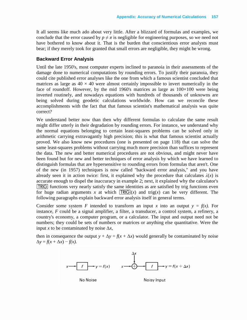
Appendix: Accuracy of Numerical Calculations 157
It all seems like much ado about very little. After a blizzard of formulas and examples, we
conclude that the error caused by p ≠ π is negligible for engineering purposes, so we need not
have bothered to know about it. That is the burden that conscientious error analysts must
bear; if they merely took for granted that small errors are negligible, they might be wrong.
Backward Error Analysis
Until the late 1950's, most computer experts inclined to paranoia in their assessments of the
damage done to numerical computations by rounding errors. To justify their paranoia, they
could cite published error analyses like the one from which a famous scientist concluded that
matrices as large as 40 × 40 were almost certainly impossible to invert numerically in the
face of roundoff. However, by the mid 1960's matrices as large as 100×100 were being
inverted routinely, and nowadays equations with hundreds of thousands of unknowns are
being solved during geodetic calculations worldwide. How can we reconcile these
accomplishments with the fact that that famous scientist's mathematical analysis was quite
correct?
We understand better now than then why different formulas to calculate the same result
might differ utterly in their degradation by rounding errors. For instance, we understand why
the normal equations belonging to certain least-squares problems can be solved only in
arithmetic carrying extravagantly high precision; this is what that famous scientist actually
proved. We also know new procedures (one is presented on page 118) that can solve the
same least-squares problems without carrying much more precision than suffices to represent
the data. The new and better numerical procedures are not obvious, and might never have
been found but for new and better techniques of error analysis by which we have learned to
distinguish formulas that are hypersensitive to rounding errors from formulas that aren't. One
of the new (in 1957) techniques is now called "backward error analysis," and you have
already seen it in action twice: first, it explained why the procedure that calculates λ(x) is
accurate enough to dispel the inaccuracy in example 2; next, it explained why the calculator's
Æ functions very nearly satisfy the same identities as are satisfied by trig functions even
for huge radian arguments x at which Æ(x) and trig(x) can be very different. The
following paragraphs explain backward error analysis itself in general terms.
Consider some system F intended to transform an input x into an output y = f(x). For
instance, F could be a signal amplifier, a filter, a transducer, a control system, a refinery, a
country's economy, a computer program, or a calculator. The input and output need not be
numbers; they could be sets of numbers or matrices or anything else quantitative. Were the
input x to be contaminated by noise Δx,
then in consequence the output y + Δy = f(x + Δx) would generally be contaminated by noise
Δy = f(x + Δx) − f(x).
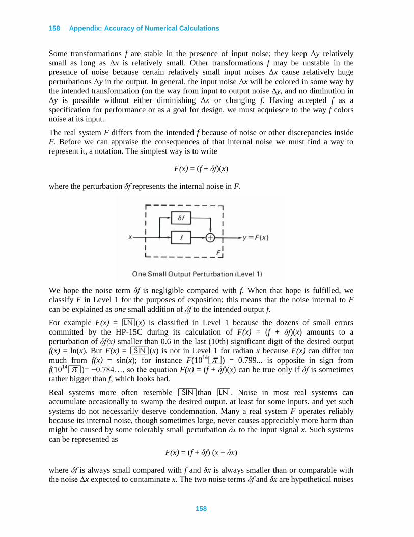
158 Appendix: Accuracy of Numerical Calculations
158
Some transformations f are stable in the presence of input noise; they keep Δy relatively
small as long as Δx is relatively small. Other transformations f may be unstable in the
presence of noise because certain relatively small input noises Δx cause relatively huge
perturbations Δy in the output. In general, the input noise Δx will be colored in some way by
the intended transformation (on the way from input to output noise Δy, and no diminution in
Δy is possible without either diminishing Δx or changing f. Having accepted f as a
specification for performance or as a goal for design, we must acquiesce to the way f colors
noise at its input.
The real system F differs from the intended f because of noise or other discrepancies inside
F. Before we can appraise the consequences of that internal noise we must find a way to
represent it, a notation. The simplest way is to write
F(x) = (f + δf)(x)
where the perturbation δf represents the internal noise in F.
We hope the noise term δf is negligible compared with f. When that hope is fulfilled, we
classify F in Level 1 for the purposes of exposition; this means that the noise internal to F
can be explained as one small addition of δf to the intended output f.
For example F(x) = N(x) is classified in Level 1 because the dozens of small errors
committed by the HP-15C during its calculation of F(x) = (f + δf)(x) amounts to a
perturbation of δf(x) smaller than 0.6 in the last (10th) significant digit of the desired output
f(x) = ln(x). But F(x) = [(x) is not in Level 1 for radian x because F(x) can differ too
much from f(x) = sin(x); for instance F(1014$) = 0.799... is opposite in sign from
f(1014$)= −0.784…, so the equation F(x) = (f + δf)(x) can be true only if δf is sometimes
rather bigger than f, which looks bad.
Real systems more often resemble [than N. Noise in most real systems can
accumulate occasionally to swamp the desired output. at least for some inputs. and yet such
systems do not necessarily deserve condemnation. Many a real system F operates reliably
because its internal noise, though sometimes large, never causes appreciably more harm than
might be caused by some tolerably small perturbation δx to the input signal x. Such systems
can be represented as
F(x) = (f + δf) (x + δx)
where δf is always small compared with f and δx is always smaller than or comparable with
the noise Δx expected to contaminate x. The two noise terms δf and δx are hypothetical noises
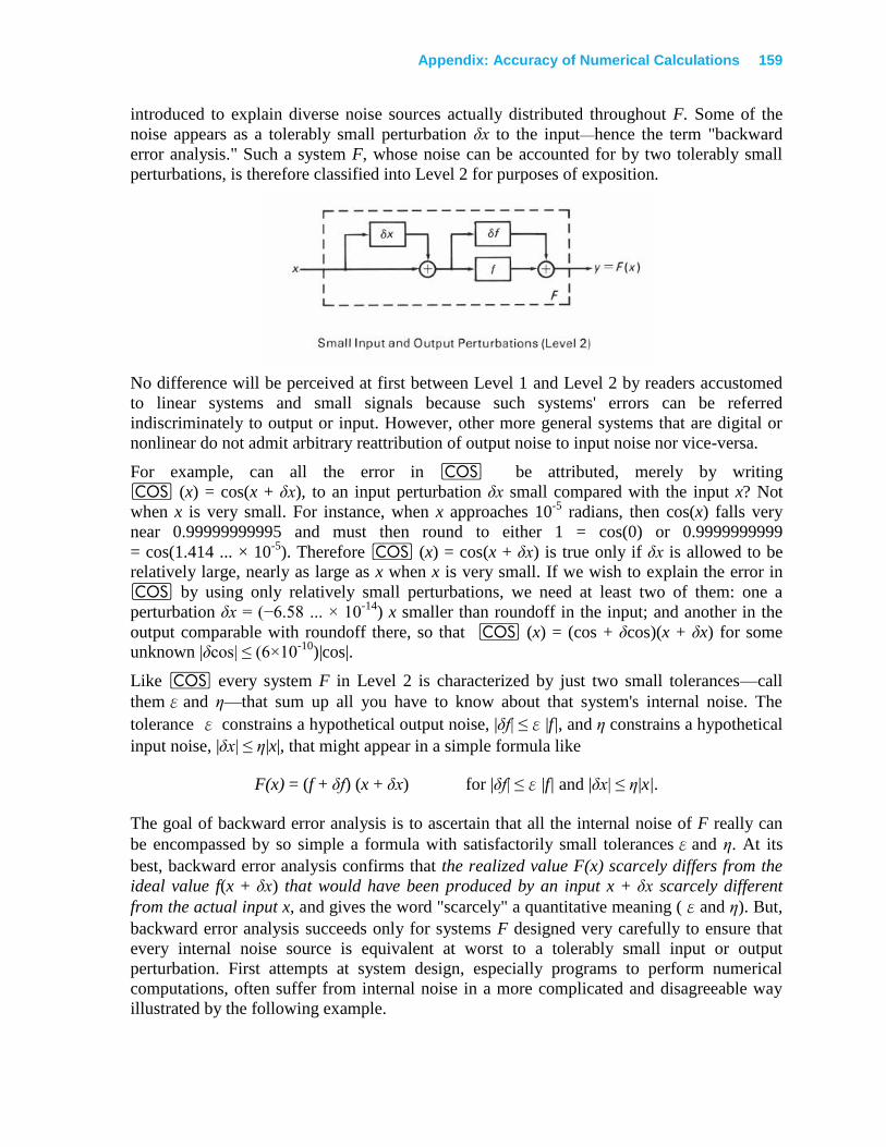
Appendix: Accuracy of Numerical Calculations 159
introduced to explain diverse noise sources actually distributed throughout F. Some of the
noise appears as a tolerably small perturbation δx to the input—hence the term "backward
error analysis." Such a system F, whose noise can be accounted for by two tolerably small
perturbations, is therefore classified into Level 2 for purposes of exposition.
No difference will be perceived at first between Level 1 and Level 2 by readers accustomed
to linear systems and small signals because such systems' errors can be referred
indiscriminately to output or input. However, other more general systems that are digital or
nonlinear do not admit arbitrary reattribution of output noise to input noise nor vice-versa.
For example, can all the error in \ be attributed, merely by writing
\ (x) = cos(x + δx), to an input perturbation δx small compared with the input x? Not
when x is very small. For instance, when x approaches 10-5
radians, then cos(x) falls very
near 0.99999999995 and must then round to either 1 = cos(0) or 0.9999999999
= cos(1.414 ... × 10-5
). Therefore \ (x) = cos(x + δx) is true only if δx is allowed to be
relatively large, nearly as large as x when x is very small. If we wish to explain the error in
\ by using only relatively small perturbations, we need at least two of them: one a
perturbation δx = (−6.58 ... × 10-14
) x smaller than roundoff in the input; and another in the
output comparable with roundoff there, so that \ (x) = (cos + δcos)(x + δx) for some
unknown |δcos| ≤ (6×10⁻¹⁰
)|cos|.
Like \ every system F in Level 2 is characterized by just two small tolerances—call
themεand η—that sum up all you have to know about that system's internal noise. The
tolerance ε constrains a hypothetical output noise, |δf| ≤ε|f|, and η constrains a hypothetical
input noise, |δx| ≤ η|x|, that might appear in a simple formula like
F(x) = (f + δf) (x + δx) for |δf| ≤ε|f| and |δx| ≤ η|x|.
The goal of backward error analysis is to ascertain that all the internal noise of F really can
be encompassed by so simple a formula with satisfactorily small tolerancesεand η. At its
best, backward error analysis confirms that the realized value F(x) scarcely differs from the
ideal value f(x + δx) that would have been produced by an input x + δx scarcely different
from the actual input x, and gives the word "scarcely" a quantitative meaning (εand η). But,
backward error analysis succeeds only for systems F designed very carefully to ensure that
every internal noise source is equivalent at worst to a tolerably small input or output
perturbation. First attempts at system design, especially programs to perform numerical
computations, often suffer from internal noise in a more complicated and disagreeable way
illustrated by the following example.
160 Appendix: Accuracy of Numerical Calculations
160
Example 6: The Smaller Root of a Quadratic. The two roots x and y of the quadratic
equation c − 2bz + az2 = 0 are real whenever d = b
2 − ac is nonnegative. Then the root y of
smaller magnitude can be regarded as a function y = f(a,b,c) of the quadratic's coefficients
otherwise. 2/)/(
0if /))sgn((),,(
bc
aabdbcbaf
Were this formula translated directly in a program F(a, b, c) intended to calculate f(a, b, c),
then whenever ac is so small compared with b2 that the computed value of d rounds to b
2,
that program could deliver F = 0 even though f ≠ 0. So drastic an error cannot be explained
by backward error analysis because no relatively small perturbations to each coefficient a, b,
and c could drive c to zero, as would be necessary to change the smaller root y into 0. On the
other hand, the algebraically equivalent formula
otherwise 0
nonzero isdivisor if ))sgn(/(),,(
bdbccbaf
translates into a much more accurate program F whose errors do no more damage than would
a perturbation in the last (10th) significant digit of c. Such a program will be listed later (page
172) and must be used in those instances, common in engineering, when the smaller root y is
needed accurately despite the fact that the quadratic's other unwanted root is relatively large.
Almost all the functions built into the HP-15C have been designed so that backward error
analysis will account for their errors satisfactorily. The exceptions are _, f, and the
statistics keys S, L, and j which can malfunction in certain pathological cases.
Otherwise, every calculator function F intended to produce f(x) produces instead a value F(x)
no farther from f(x) than if first x had been perturbed to x+δx with |δx| ≤ η|x|, then f(x+δx)
were perturbed to(f+δf)(x+δx) with|δf| ≤ ε|f|. The tolerances η and ε vary a little from function
to function; roughly speaking
η = 0 and ε < 10-9
for all functions in Level 1,
η < 10-12
and ε < 6×10⁻¹⁰
for all real and complex functions.
For matrix operations, the magnitudes |δx|, |x|, |δf|, and |f| replaced by matrix norms ||δx||, ||x||,
||δf||, and ||f|| respectively, which are explained in section 4 and evaluated using > 7 or
> 8. Then all matrix functions not in Level 1 fall into Level 2 with roughly
η ≤ 10-12
n and ε < 10-9
for all matrix operations (other than
determinant > 9, ÷, ⁄)
η < 10-9
n and ε < 10-9
for determinant > 9, ⁄,
and ÷ with matrix divisor
where n is the largest dimension of any matrix involved in the operation.
The implications of successful backward error analysis look simple only when the input data
x comes contaminated by unavoidable and uncorrelated noise Δx, as is often the case. Then
Appendix: Accuracy of Numerical Calculations 161
when we wish to calculate f(x), the best we could hope to get is f(x + Δx), but we actually get
F(x+Δx)=(f+δf)(x+Δx+δx), where |δf| ≤ ε|f| and |δx| ≤ η|x|.
What we get is scarcely worse than the best we could hope for provided the tolerances ε and
η are small enough, particularly if |Δx| is likely to be at least roughly as big as η|x|. Of course,
the best we could hope for may be very bad, especially if f possesses a singularity closer to x
than the tolerances upon x's perturbation Δx and δx.
Backward Error Analysis Versus Singularities
The word "singularity" refers to both a special value of the argument x and to the way f(x)
misbehaves as x approaches that special value. Most commonly, f(x) or its first derivative
f'(x) may become infinite or violently oscillatory as x approaches the singularity. Sometimes
the singularities of ln|f| are called singularities of f, thereby including the zeros of f among its
singularities; this makes sense when the relative accuracy of a computation of f is at issue, as
we shall see. For our purposes the meaning of "singularity" can be left a little vague.
What we usually want to do with singularities is avoid or neutralize them. For instance, the
function
otherwise 21
0 if 2cos1 )(
xxxxc
has no singularity at x = 0 even though its constituents 1 − cos x and x2 (actually, their
logarithms) do behave singularly as x approaches 0. The constituent singularities cause
trouble for the program that calculates c(x). Most of the trouble is neutralized by the choice
of a better formula
otherwise. 21
02 if
2
2
2sin
2
1)( x
x
xxc
Now the singularity can be avoided entirely by testing whether x/2 = 0 in the program that
calculates c(x).
Backward error analysis complicates singularities in a way that is easiest to illustrate with the
function λ(x) = ln(1 + x) that solved the savings problem in example 2. The procedure used
there calculated u = 1 + x (rounded) = 1 + x + Δx. Then
otherwise. )1()ln(
1u if )(
uxu
xx
This procedure exploits the fact that λ(x)/x has a removable singularity at x = 0, which means
that λ(x)/x varies continuously and approaches 1 as x approaches 0. Therefore, λ(x)/x is
relatively closely approximated by λ(x+Δx) / (x+Δx) when |Δx| < 10-9
, and hence
λ(x) = x(λ(x)/x) ≈ x(λ(x+Δx)/(x+Δx)) = x(ln(u)/(u−1)),
162 Appendix: Accuracy of Numerical Calculations
162
all calculated accurately because N is in Level 1. What might happen if N were in Level
2 instead?
If N were in Level 2, then "successful" backward error analysis would show that, for
arguments u near 1, N (u) = ln(u +δu) with |δu| < 10-9
. Then the procedure above would
produce not x(ln(u)/(u−1)), but
.1)(
1)(
)(
)(
)(
1
)ln(
xx
ux
xx
u
x
xx
xx
uxx
uxx
uxxx
xx
uxxx
u
uux
When |x+Δx| is not much bigger than 10-9
, the last expression can be utterly different from λ
(x). Therefore, the procedure that solved example 2 would fail on machines whose N is not
in Level 1. There are such machines, and on them the procedure does collapse for certain
otherwise innocuous inputs. Similar failures also occur on machines that produce (u+δ’u) − 1
instead of u − 1 because their - function lies in Level 2 instead of Level 1. And those
machines that produce ln(u + δu )/(u + δ’u − 1) instead of ln(u)/(u − 1), because both N
and - lie in Level 2, would be doubly vulnerable but for an ill-understood accident that
usually correlates the two backward errors δu and δ’u in such a way as causes only half the
significant digits of the computed λ, instead of all of them, to be wrong.
Summary to Here
Now that the complexity injected by backward error analysis into singularities has been
exposed, the time has come to summarize, to simplify, and to consolidate what has been
discussed so far.
Many numerical procedures produce results too wrong to be justified by any
satisfactory error analysis, backward or not.
Some numerical procedures produce results only slightly worse than would have been
obtained by exactly solving a problem differing only slightly from the given problem.
Such procedures, classified in Level 2 for our purposes, are widely accepted as
satisfactory from the point of view of backward error analysis.
Procedures in Level 2 can produce results relatively far from what would have been
obtained had no errors at all been committed, but large errors can result only for data
relatively near a singularity of the function being computed.
Procedures in Level 1 produce relatively accurate results regardless of near approach to
a singularity. Such procedures are rare, but preferable if only because their results are
easier to interpret, especially when several variables are involved.
A simple example illustrates all four points.
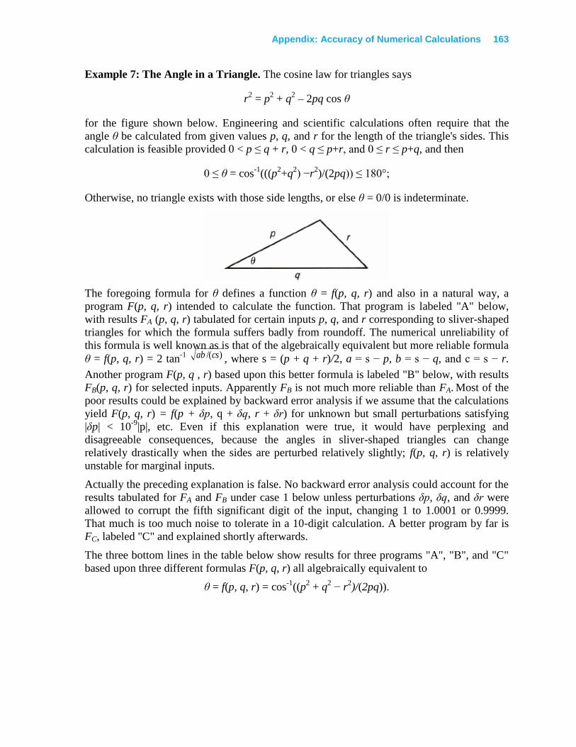
Appendix: Accuracy of Numerical Calculations 163
Example 7: The Angle in a Triangle. The cosine law for triangles says
r2 = p
2 + q
2 – 2pq cos θ
for the figure shown below. Engineering and scientific calculations often require that the
angle θ be calculated from given values p, q, and r for the length of the triangle's sides. This
calculation is feasible provided 0 < p ≤ q + r, 0 < q ≤ p+r, and 0 ≤ r ≤ p+q, and then
0 ≤ θ = cos-1
(((p2+q
2) −r
2)/(2pq)) ≤ 180°;
Otherwise, no triangle exists with those side lengths, or else θ = 0/0 is indeterminate.
The foregoing formula for θ defines a function θ = f(p, q, r) and also in a natural way, a
program F(p, q, r) intended to calculate the function. That program is labeled "A" below,
with results FA (p, q, r) tabulated for certain inputs p, q, and r corresponding to sliver-shaped
triangles for which the formula suffers badly from roundoff. The numerical unreliability of
this formula is well known as is that of the algebraically equivalent but more reliable formula
θ = f(p, q, r) = 2 tan-1
)/(csab , where s = (p + q + r)/2, a = s − p, b = s − q, and c = s − r.
Another program F(p, q , r) based upon this better formula is labeled "B" below, with results
FB(p, q, r) for selected inputs. Apparently FB is not much more reliable than FA. Most of the
poor results could be explained by backward error analysis if we assume that the calculations
yield F(p, q, r) = f(p + δp, q + δq, r + δr) for unknown but small perturbations satisfying
|δp| < 10-9
|p|, etc. Even if this explanation were true, it would have perplexing and
disagreeable consequences, because the angles in sliver-shaped triangles can change
relatively drastically when the sides are perturbed relatively slightly; f(p, q, r) is relatively
unstable for marginal inputs.
Actually the preceding explanation is false. No backward error analysis could account for the
results tabulated for FA and FB under case 1 below unless perturbations δp, δq, and δr were
allowed to corrupt the fifth significant digit of the input, changing 1 to 1.0001 or 0.9999.
That much is too much noise to tolerate in a 10-digit calculation. A better program by far is
FC, labeled "C" and explained shortly afterwards.
The three bottom lines in the table below show results for three programs "A", "B", and "C"
based upon three different formulas F(p, q, r) all algebraically equivalent to
θ = f(p, q, r) = cos-1
((p2 + q
2 − r
2)/(2pq)).
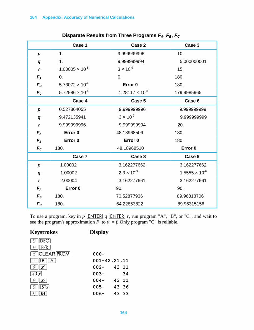
164 Appendix: Accuracy of Numerical Calculations
164
Disparate Results from Three Programs FA, FB, FC
Case 1 Case 2 Case 3
p 1. 9.999999996 10.
q 1. 9.999999994 5.000000001
r 1.00005 × 10⁻⁵ 3 × 10⁻⁹ 15.
FA 0. 0. 180.
FB 5.73072 × 10⁻⁴ Error 0 180.
FC 5.72986 × 10⁻⁴ 1.28117 × 10⁻⁸ 179.9985965
Case 4 Case 5 Case 6
p 0.527864055 9.999999996 9.999999999
q 9.472135941 3 × 10⁻⁹ 9.999999999
r 9.999999996 9.999999994 20.
FA Error 0 48.18968509 180.
FB Error 0 Error 0 180.
FC 180. 48.18968510 Error 0
Case 7 Case 8 Case 9
p 1.00002 3.162277662 3.162277662
q 1.00002 2.3 × 10⁻⁹ 1.5555 × 10⁻⁶
r 2.00004 3.162277661 3.162277661
FA Error 0 90. 90.
FB 180. 70.52877936 89.96318706
FC 180. 64.22853822 89.96315156
To use a program, key in p v q v r, run program "A", "B", or "C", and wait to
see the program's approximation F to θ = f. Only program "C" is reliable.
Keystrokes Display
|D
|¥
´CLEARM 000-
´bA 001-42,21,11
|x 002- 43 11
® 003- 34
|x 004- 43 11
|K 005- 43 36
|( 006- 43 33
Appendix: Accuracy of Numerical Calculations 165
Keystrokes Display
* 007- 20
® 008- 34
|K 009- 43 36
|x 010- 43 11
+ 011- 40
|( 012- 43 33
- 013- 30
® 014- 34
v 015- 36
+ 016- 40
÷ 017- 10
|{ 018- 43 24
|n 019- 43 32
´bB 020-42,21,12
O1 021- 44 1
v 022- 36
|( 023- 43 33
O+1 024-44,40, 1
|( 025- 43 33
O+1 026-44,40, 1
2 027- 2
O÷1 028-44,10, 1
) 029- 33
l-1 030-45,30, 1
® 031- 34
l-1 032-45,30, 1
* 033- 20
¤ 034- 11
® 035- 34
l-1 036-45,30, 1
l*1 037-45,20, 1
” 038- 16
¤ 039- 11
|: 040- 43 1
) 041- 33
* 042- 20
|n 043- 43 32
´bC 044-42,21,13
O0 045- 44 0
166 Appendix: Accuracy of Numerical Calculations
166
Keystrokes Display
) 046- 33
|£ 047- 43 10
® 048- 34
O1 049- 44 1
O+0 050-44,40, 0
® 051- 34
O+0 052-44,40, 0
- 053- 30
|( 054- 43 33
O-1 055-44,30, 1
|K 056- 43 36
v 057- 36
l+1 058-45,40, 1
¤ 059- 11
´X0 060-42, 4, 0
¤ 061- 11
O*0 062-44,20, 0
|` 063- 43 35
+ 064- 40
) 065- 33
+ 066- 40
´X1 067-42, 4, 1
|( 068- 43 33
|K 069- 43 36
|£ 070- 43 10
t.9 071- 22 .9
) 072- 33
|T2 073-43,30, 2
¤ 074- 11
® 075- 34
t.8 076- 22 .8
´b.9 077-42,21,.9
|T2 078-43,30, 2
¤ 079- 11
|( 080- 43 33
´b.8 081-42,21,.8
- 082- 30
¤ 083- 11
l1 084- 45 1
Appendix: Accuracy of Numerical Calculations 167
Keystrokes Display
¤ 085- 11
* 086- 20
l0 087- 45 0
|: 088- 43 1
|~ 089- 43 20
÷ 090- 10
® 091- 34
v 092- 36
+ 093- 40
|n 094- 43 32
|¥
The results FC(p, q , r) are correct to at least nine significant digits. They are obtained from a
program "C" that is utterly reliable though rather longer than the unreliable programs "A" and
"B". The method underlying program "C" is:
1. If p < q, then swap them to ensure p ≥ q.
2. Calculate b=(p−q)+r, c=(p−r)+q, and s=(p+r)+q.
3. Calculate
exists). triangle(no otherwise
0 if )(
0if )(
0 Error
qrrpq
r qqpr
a
4. Calculate FC(p, q, r) = 2 tan-1
( csab ).
This procedure delivers FC(p, q, r) = θ correct to almost nine significant digits, a result surely
easier to use and interpret than the results given by the other better-known formulas. But this
procedure's internal workings are hard to explain; indeed, the procedure may malfunction on
some calculators and computers.
The procedure works impeccably on only certain machines like the HP-15C, whose
subtraction operation is free from avoidable error and therefore enjoys the following
property: Whenever y lies between x/2 and 2x, the subtraction operation introduces no
roundoff error into the calculated value of x − y. Consequently, whenever cancellation might
leave relatively large errors contaminating a, b, or c, the pertinent difference (p − q) or (p − r)
turns out to be free from error, and then cancellation turns out to be advantageous!
Cancellation remains troublesome on those other machines that calculate (x +δx) − (y + δy)
instead of x − y even though neither δx nor δy amounts to as much as one unit in the last
significant digit carried in x or y respectively. Those machines deliver FC(p, q, r) = f(p + δp,
q + δq, r + δr) with end-figure perturbations δp , δq, and δr that always seem negligible from
the viewpoint of backward error analysis, but which can have disconcerting consequences.
For instance, only one of the triples (p, q, r) or (p + δp, q + δq, r + δr), not both, might
168 Appendix: Accuracy of Numerical Calculations
168
constitute the edge lengths of a feasible triangle, so FC might produce an error message when
it shouldn't, or vice-versa, on those machines.
Backward Error Analysis of Matrix Inversion
The usual measure of the magnitude of a matrix X is a norm ||X|| such as is calculated by
either >7 or >8; we shall use the former norm, the row norm
j
ijxi
maxX
in what follows. This norm has properties similar to those of the length of a vector and also
the multiplicative property
||XY|| ≤ ||X|| ||Y|| .
When the equation Ax = b is solved numerically with a given n × n matrix A and column
vector b, the calculated solution is a column vector c which satisfies nearly the same equation
as does x, namely
(A + δA) c = b
with ||δA|| < 10-9
n ||A||.
Consequently the residual b − Ac = (δA)c is always relatively small; quite often the residual
norm ||b − Ac|| smaller than xAb where x is obtained from the true solution x by
rounding each of its elements to 10 significant digits. Consequently, c can differ significantly
from x only if A is nearly singular, or equivalently only if ||A-1
|| is relatively large compared
with 1/||A||;
||x − c|| = ||A-1
(b − Ac)||
≤ ||A-1
|| ||δA|| ||c||
≤ 10-9
n ||c|| / σ(A)
where σ(A) = 1/(||A|| ||A-1
||) is the reciprocal of the condition number and measures how
relatively near to A is the nearest singular matrix S, since
.σ0)det(
min A(A)SAS
These relations and some of their consequences are discussed extensively in section 4.
The calculation of A-1
is more complicated. Each column of the calculated inverse ⁄(A) is
the corresponding column of some (A+δA)-1
, but each column has its own small δA.
Consequently, no single small δA, with ||δA||≤10-9
n ||A||, need exist satisfying
||(A+ δA)-1
− ⁄ (A)|| ≤ 10-9
||⁄ (A)||
roughly. Usually such a δA exists, but not always. This does not violate the prior assertion
that the matrix operations ⁄and ÷ lie in Level 2; they are covered by the second
assertion of the summary on page 162. The accuracy of ⁄ (A) can be described in terms of
the inverses of all matrices A + ΔA so near A that ||ΔA|| ≤ 10-9
n||A||; the worst among those
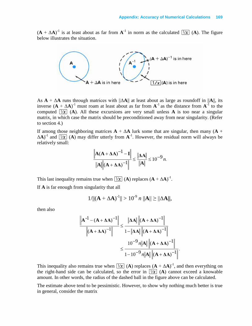
Appendix: Accuracy of Numerical Calculations 169
(A + ΔA)-1
is at least about as far from A-1
in norm as the calculated ⁄ (A). The figure
below illustrates the situation.
As A + ΔA runs through matrices with ||ΔA|| at least about as large as roundoff in ||A||, its
inverse (A + ΔA)-1
must roam at least about as far from A-1
as the distance from A-1
to the
computed ⁄ (A). All these excursions are very small unless A is too near a singular
matrix, in which case the matrix should be preconditioned away from near singularity. (Refer
to section 4.)
If among those neighboring matrices A + ΔA lurk some that are singular, then many (A +
ΔA)-1
and ⁄ (A) may differ utterly from A-1
. However, the residual norm will always be
relatively small:
.910
1)(
1)(n
A
ΔA
ΔAAA
IΔAAA
This last inequality remains true when ⁄ (A) replaces (A + ΔA)-1
.
If A is far enough from singularity that all
1/||(A + ΔA)-1
|| > 10-9
n ||A|| ≥ ||ΔA||,
then also
.1)(9101
1)(910
1)(1
1)(
1)(
1)(1
ΔAAA
ΔAAA
ΔAAΔA
ΔAAΔA
ΔAA
ΔAAA
n
n
-
This inequality also remains true when ⁄ (A) replaces (A + ΔA)-1
, and then everything on
the right-hand side can be calculated, so the error in ⁄ (A) cannot exceed a knowable
amount. In other words, the radius of the dashed ball in the figure above can be calculated.
The estimate above tend to be pessimistic. However, to show why nothing much better is true
in general, consider the matrix
170 Appendix: Accuracy of Numerical Calculations
170
000,52000
03.000,5000002.000
4503.000,50000,500
4503.000,5000050000020 ,.
X
and
692300001923070000
95192076480005000
980770764803000500000200
0005000050
1
.
.,,
.,.,.
qp,,
-X
Ideally, p = q = 0, but the HP-15C's approximation to X-1
, namely ⁄ (X), has
q = 9.643.269231 instead, a relative error
,0964.0)(
1
1
X
XX
Nearly 10 percent. On the other hand, if X + ΔX differs from X only in its second column
where −50,000 and 50,000 are replaced respectively by −50,000.000002 and 49,999.999998
(altered in the 11th significant digit), then (X + ΔX)-1
differs significantly from X-1
only
insofar as p = 0 and q = 0 must be replaced by p = 10,000.00600 ... and q = 9,615.396154 ....
Hence,
;196.0
1
11
X
ΔXXX
the relative error in (X + ΔX)-1
is nearly twice that in ⁄ (X). Do not try to calculate (X +
ΔX)-1
directly. but use instead the formula
(X − cbT)
-1 = X
-1 + X
-1cb
TX
-1 / (1 − b
TX
-1c),
which is valid for any column vector c and row vector bT, and specifically for
0
0
1
1
c and 00000002.00Tb .
Despite that
||X-1
− ⁄ (X)|| < ||X-1
− (X+ ΔX)-1
|| ,
it can be shown that no very small end-figure perturbation δX exists for which (X + δX)-1
matches ⁄ (X) to more than five significant digits in norm.
⁄
Appendix: Accuracy of Numerical Calculations 171
Of course, none of these horrible things could happen if X were not so nearly singular.
Because ||X|| ||X-1
|| > 1010
, a change in X amounting to less than one unit in the 10th
significant digit of ||X|| could make X singular; such a change might replace one of the
diagonal elements 0.00002 of X by zero. Since X is so nearly singular, the accuracy ⁄(X)
in this case rather exceeds what might be expected in general. What makes this example
special is bad scaling; X was obtained from an unexceptional matrix
25000
0000035200
1054000003550
10540000035502
~12
12
.
..
...
....
X
by multiplying each row and each column by a carefully chosen power of 10. Compensatory
division of the columns and rows of the equally unexceptional matrix
19230769230000
480769519205000
480769807700000035200
5050
~ 1
.
..
...
qp..
-X
yielded X-1
, with p = q = 0. The HP-15C calculates ⁄( X~
) = X~ -1
except that q = 0 is
replaced by q = 9.6×10⁻¹¹
, a negligible change. This illustrates how drastically the perceived
quality of computed results can be altered by scaling. (Refer to section 4 for more
information about scaling.)
Is Backward Error Analysis a Good Idea?
The only good thing to be said for backward error analysis is that it explains internal errors in
a way that liberates a system's user from having to know about internal details of the system.
Given two tolerances, one upon the input noise s« and one upon the output noise δf, the user
can analyze the consequences of internal noise In
F(x) = (f + δf) (x + δx)
by studying the noise propagation properties of the ideal system f without further reference to
the possibly complex internal structure of F.
But backward error analysis is no panacea; it may explain errors but not excuse them.
Because it complicates computations involving singularities, we have tried to eliminate the
need for it wherever we could. If we knew how to eliminate the need for backward error
analysis from every function built into the calculator, and to do so at tolerable cost, we would
do that and simplify life for everyone. That simplicity would cost too much speed and
memory for today's technology. The next example will illustrate the trade-offs involved.
172 Appendix: Accuracy of Numerical Calculations
172
Example 6 Continued. The program listed below solves the real quadratic equation c − 2 bz
+ az2 = 0 for real or complex roots.
To use the program, key the real constants into the stack (c v b v a) and run
program "A".
The roots x and y will appear in the X- and Y-registers. If the roots are complex, the C
annunciator turns on, indicating that Complex mode has been activated. The program uses
labels "A" and ".9" and the Index register (but none of the other registers 0 to .9); therefore,
the program may readily be called as a subroutine by other programs. The calling programs
(after clearing flag 8 if necessary) can discover whether roots are real or complex by testing
flag 8, which gets set only if roots are complex.
The roots x and y are so ordered that |x| ≥ |y| except possibly when |x| and |y| agree to more
than nine significant digits. The roots are as accurate as if the coefficient c had first been
perturbed in its 10th significant digit, the perturbed equation had been solved exactly, and its
roots rounded to 10 significant digits. Consequently, the computed roots match the given
quadratic's roots to at least five significant digits. More generally, if the roots x and y agree to
n significant digits for some positive n ≤ 5, then they are correct to at least 10 − n significant
digits unless overflow or underflow occurs.
Keystrokes Display
|¥
´CLEARM 000-
´bA 001-42,21,11
v 002- 36
|( 003- 43 33
* 004- 20
|K 005- 43 36
® 006- 34
|( 007- 43 33
OV 008- 44 25
|x 009- 43 11
- 010- 30
|T1 011-43,30, 1
t.9 012- 22 .9
” 013- 16
¤ 014- 11
´XV 015-42, 4,25
|T2 016-43,30, 2
l-V 017-45,30,25
|T3 018-43,30, 3
l+V 019-45,40,25
|T0 020-43,30, 0
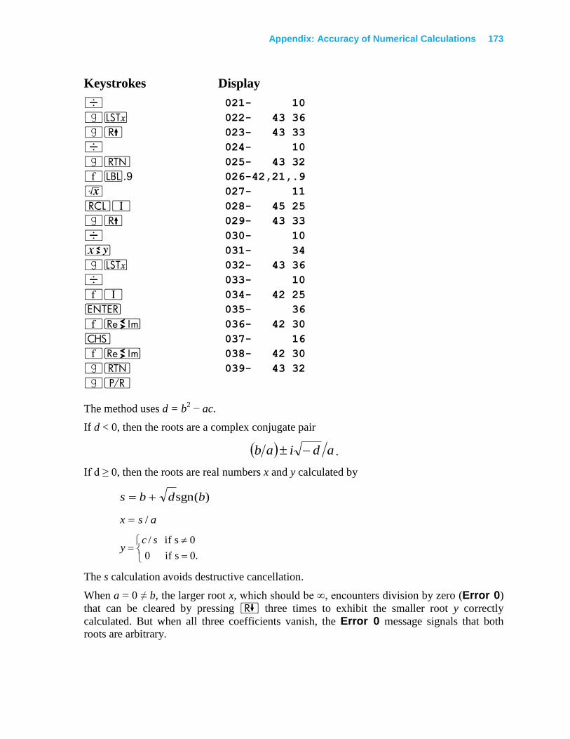
Appendix: Accuracy of Numerical Calculations 173
Keystrokes Display
÷ 021- 10
|K 022- 43 36
|( 023- 43 33
÷ 024- 10
|n 025- 43 32
´b.9 026-42,21,.9
¤ 027- 11
lV 028- 45 25
|( 029- 43 33
÷ 030- 10
® 031- 34
|K 032- 43 36
÷ 033- 10
´V 034- 42 25
v 035- 36
´} 036- 42 30
” 037- 16
´} 038- 42 30
|n 039- 43 32
|¥
The method uses d = b2 − ac.
If d < 0, then the roots are a complex conjugate pair
adiab .
If d ≥ 0, then the roots are real numbers x and y calculated by
)(sgn bdbs
asx /
0.s if 0
0s if / scy
The s calculation avoids destructive cancellation.
When a = 0 ≠ b, the larger root x, which should be ∞, encounters division by zero (Error 0)
that can be cleared by pressing ) three times to exhibit the smaller root y correctly
calculated. But when all three coefficients vanish, the Error 0 message signals that both
roots are arbitrary.
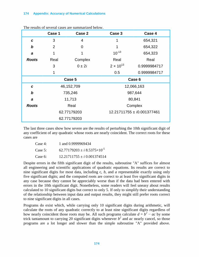
174 Appendix: Accuracy of Numerical Calculations
174
The results of several cases are summarized below.
Case 1 Case 2 Case 3 Case 4
c 3 4 1 654,321
b 2 0 1 654,322
a 1 1 10-13 654,323
Roots Real Complex Real Real
3 0 ± 2i 2 × 10¹³ 0.9999984717
1 0.5 0.9999984717
Case 5 Case 6
c 46,152,709 12,066,163
b 735,246 987,644
a 11,713 80,841
Roots Real Complex
62.77179203 12.21711755 ± i0.001377461
62.77179203
The last three cases show how severe are the results of perturbing the 10th significant digit of
any coefficient of any quadratic whose roots are nearly coincident. The correct roots for these
cases are
Case 4: 1 and 0.9999969434
Case 5: 62.77179203 ± i 8.5375×10⁻⁵
Case 6: 12.21711755 ± i 0.001374514
Despite errors in the fifth significant digit of the results, subroutine "A" suffices for almost
all engineering and scientific applications of quadratic equations. Its results are correct to
nine significant digits for most data, including c, b, and a representable exactly using only
five significant digits; and the computed roots are correct to at least five significant digits in
any case because they cannot be appreciably worse than if the data had been entered with
errors in the 10th significant digit. Nonetheless, some readers will feel uneasy about results
calculated to 10 significant digits but correct to only 5. If only to simplify their understanding
of the relationship between input data and output results, they might still prefer roots correct
to nine significant digits in all cases.
Programs do exist which, while carrying only 10 significant digits during arithmetic, will
calculate the roots of any quadratic correctly to at least nine significant digits regardless of
how nearly coincident those roots may be. All such programs calculate d = b2 − ac by some
trick tantamount to carrying 20 significant digits whenever b2 and ac nearly cancel, so those
programs are a lot longer and slower than the simple subroutine "A" provided above.
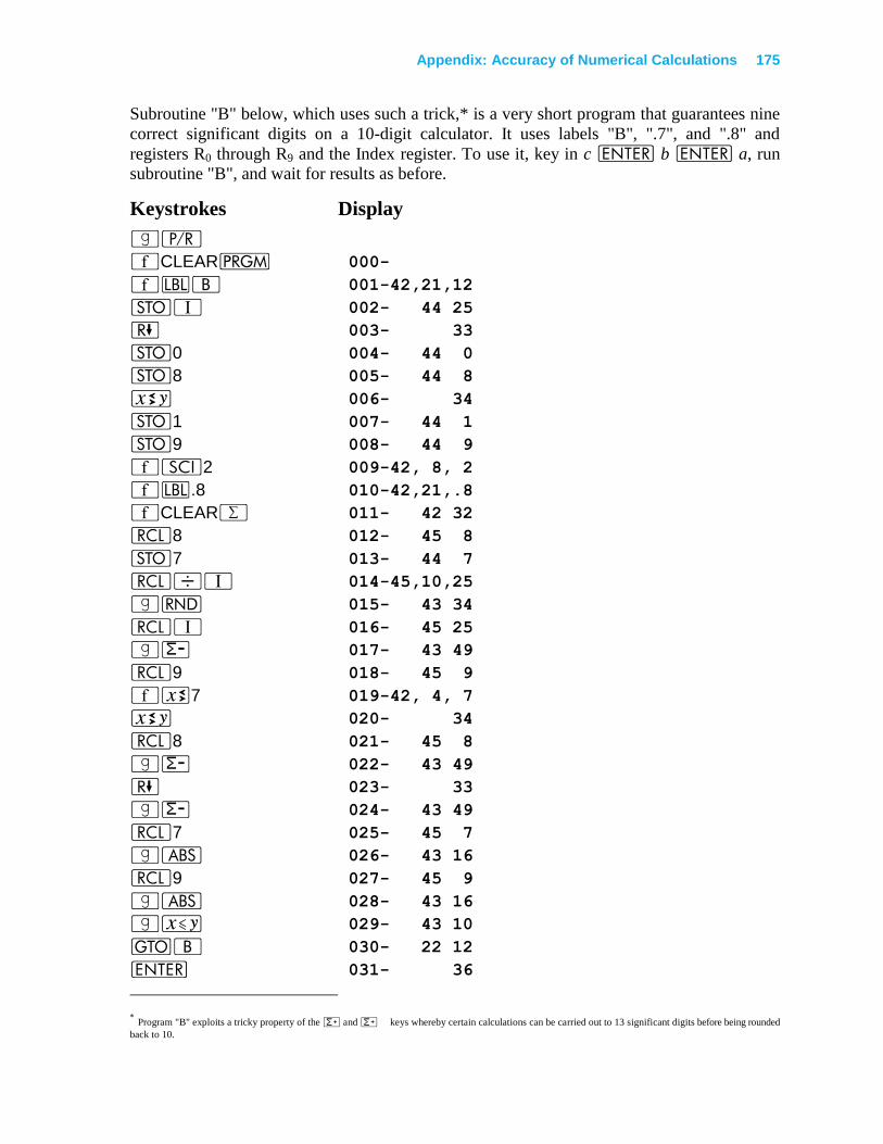
Appendix: Accuracy of Numerical Calculations 175
Subroutine "B" below, which uses such a trick,* is a very short program that guarantees nine
correct significant digits on a 10-digit calculator. It uses labels "B", ".7", and ".8" and
registers R0 through R9 and the Index register. To use it, key in c v b v a, run
subroutine "B", and wait for results as before.
Keystrokes Display
|¥
´CLEARM 000-
´bB 001-42,21,12
OV 002- 44 25
) 003- 33
O0 004- 44 0
O8 005- 44 8
® 006- 34
O1 007- 44 1
O9 008- 44 9
´i2 009-42, 8, 2
´b.8 010-42,21,.8
´CLEAR∑ 011- 42 32
l8 012- 45 8
O7 013- 44 7
l÷V 014-45,10,25
|& 015- 43 34
lV 016- 45 25
|w 017- 43 49
l9 018- 45 9
´X7 019-42, 4, 7
® 020- 34
l8 021- 45 8
|w 022- 43 49
) 023- 33
|w 024- 43 49
l7 025- 45 7
|a 026- 43 16
l9 027- 45 9
|a 028- 43 16
|£ 029- 43 10
tB 030- 22 12
v 031- 36
* Program "B" exploits a tricky property of the z and z keys whereby certain calculations can be carried out to 13 significant digits before being rounded
back to 10.
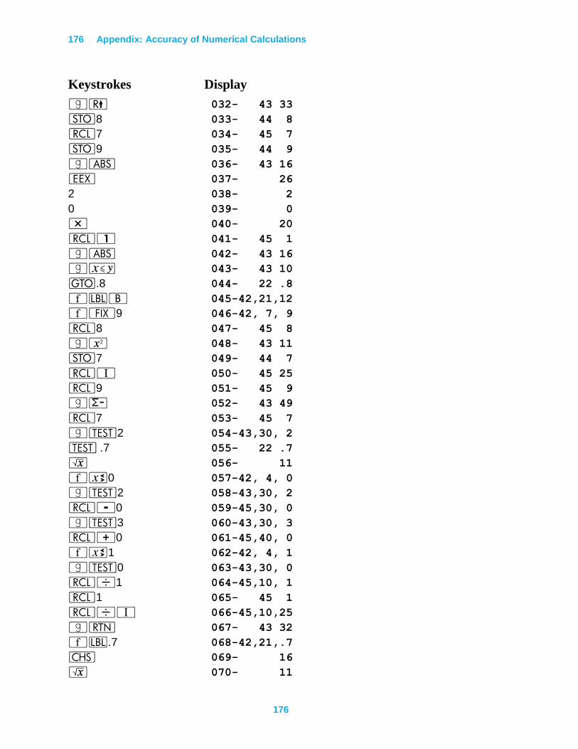
176 Appendix: Accuracy of Numerical Calculations
176
Keystrokes Display
|( 032- 43 33
O8 033- 44 8
l7 034- 45 7
O9 035- 44 9
|a 036- 43 16
“ 037- 26
2 038- 2
0 039- 0
* 040- 20
l1 041- 45 1
|a 042- 43 16
|£ 043- 43 10
t.8 044- 22 .8
´bB 045-42,21,12
´•9 046-42, 7, 9
l8 047- 45 8
|x 048- 43 11
O7 049- 44 7
lV 050- 45 25
l9 051- 45 9
|w 052- 43 49
l7 053- 45 7
|T2 054-43,30, 2
T .7 055- 22 .7
¤ 056- 11
´X0 057-42, 4, 0
|T2 058-43,30, 2
l-0 059-45,30, 0
|T3 060-43,30, 3
l+0 061-45,40, 0
´X1 062-42, 4, 1
|T0 063-43,30, 0
l÷1 064-45,10, 1
l1 065- 45 1
l÷V 066-45,10,25
|n 067- 43 32
´b.7 068-42,21,.7
” 069- 16
¤ 070- 11
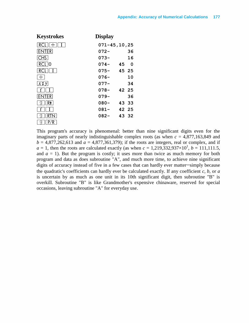
Appendix: Accuracy of Numerical Calculations 177
Keystrokes Display
l÷V 071-45,10,25
v 072- 36
” 073- 16
l0 074- 45 0
lV 075- 45 25
÷ 076- 10
® 077- 34
´V 078- 42 25
v 079- 36
|( 080- 43 33
´V 081- 42 25
|n 082- 43 32
|¥
This program's accuracy is phenomenal: better than nine significant digits even for the
imaginary parts of nearly indistinguishable complex roots (as when c = 4,877,163,849 and
b = 4,877,262,613 and a = 4,877,361,379); if the roots are integers, real or complex, and if
a = 1, then the roots are calculated exactly (as when c = 1,219,332,937×101, b = 111,111.5,
and a = 1). But the program is costly; it uses more than twice as much memory for both
program and data as does subroutine "A", and much more time, to achieve nine significant
digits of accuracy instead of five in a few cases that can hardly ever matter−simply because
the quadratic's coefficients can hardly ever be calculated exactly. If any coefficient c, b, or a
is uncertain by as much as one unit in its 10th significant digit, then subroutine "B" is
overkill. Subroutine "B" is like Grandmother's expensive chinaware, reserved for special
occasions, leaving subroutine "A" for everyday use.
178
Index
Page numbers in bold type indicate primary references; page numbers in regular type indicate
secondary references.
A
Absolute error · 146, 153, 154
Accuracy
in Complex mode · 63–65
of integrand · 41–43
of numerical calculations · 145–177
of solutions to linear system · 87–88
Aliasing · 41
Analysis of variance · 113–118
Analysis, discounted cash flow · 34–39
Angle in triangle · 163–168
Annuities · 24–34
Annuity due · 25
Annuity, ordinary · 25
Annunciator, C · 172
Annunciator, trig mode · 58
ANOVA table · 113, 118
Augmented matrix · 118
Augmented normal equations · 94
Augmented system · 120
B
Backward error analysis · 157–161
Balloon payment · 25, 27, 32
Binomial theorem · 148
Bounding search · 136, 137, 141, 143
Branch, principal · 59–62
Bridge too short · 146
Broken calculator · 145
C
Calculation time, f · 43–48
Calculations, numerical accuracy · 145–177
Cancellation · 148, 149, 152, 167, 173
Cash flow analysis, discounted · 34–39
Cash flow diagram · 25–39
Characteristic equation · 69, 125
Column norm · 84
Complementary error function · 51–55
Index 179
Complementary normal distribution function · 51–55
Complex components, accurate · 64
Complex equations, solving large system · 107–110
Complex math functions · 59–62
Complex mode · 56–81
_ and f · 63
accuracy · 63–65
Complex multivalued functions · 59–62
Complex number, n th roots · 59, 67–69
Complex number, storing and recalling · 65–66
Complex potential function · 76–81
Complex relative error · 154
Complex roots of equation · 69–73, 17–18
Complex roots of quadratic equation · 171–177
Complex single-valued functions · 59
Components, accurate complex · 64
Compound amounts · 24–34
Condition number · 84–87, 91, 92, 168
Conformal mapping · 76
Constrained least-squares · 94, 97, 120
Consumer price index · 116
Contour integral · 73–76
Correctly rounded result · 150–53
perturbed input · 154–77
Covariance matrix · 111, 112, 115
Critical point · 135, 137
D
Declination · 13–15
Decomposition, LU · 82–83
descriptor · 83
Deflation · 12
Degrees of freedom · 104, 112
Delay equation · 69–73
Derivative · 12
Descartes' Rule of Signs · 12–13
Descriptor of LU decomposition · 83
Determinant · 82–83, 99
Diagram, cash flow · 25–39
Discounted cash flow and analysis · 34–39
Discounted rate of return · 35
Display format · 40–43
Doolittle method · 83
E
Eigenvalue · 125–35
storage · 135
Eigenvector · 125, 130–35
180 Index
180
Electrostatic field · 50
Endpoint, f sampling at · 41, 48
Equations
complex, solving large system · 107–110
equivalent · 11–12
solving inaccurate · 12
solving nonlinear system · 102–107
with several roots · 12
Equipotential lines · 76–81
Equivalent equations · 11–12
Error · 145
absolute · 146, 153
hierarchy · 150
in matrix elements · 84
misconceptions · 145–149
relative · 146, 151
Error 0 · 27, 164, 167, 173
Error 1 · 137, 141
Error 4 · 26, 27, 35
Error 8 · 11, 22
Error analysis, backward · 157–161
Example
angle in triangle · 163–168
annuities · 31–34
bridge too short · 146
broken calculator · 145
cash flow · 38–39
compound amounts · 31–34
consumer price index regression · 116–118
contour integral · 75–76
declination of sun · 13–15
delay equation · 69–73
eigenvectors · 133–134
equipotential line · 81
field Intensity of antenna · 18–24
filter network · 107–110
Gamma function · 56–58
lunar phases · 156
n th root of complex number · 68
normal distribution function · 42, 55
optimizing box · 141–43
pennies · 145–46
pi · 146
quadratic surface · 129–30
residual correction · 101–2
roots of quadratic equation · 160, 171–77
storing and recalling complex numbers · 65–66
streamline · 79–80
subdividing interval of integration · 44–46
transformation of variables · 47–48
unbiased test of hypothesis · 103–7
Index 181
Extended precision · 41
Extremes of function · 18–24
F
F actorization, orthogonal · 95–98, 118–25
F ratio · 112–18
Field Intensity · 18–24
Financial equation · 26
Financial problems · 24–39
Format, display · 40–41, 42
Frobenius norm · 84
Functions, complex · 59–62
G
Gamma function, complex · 56–58
Gradient · 135, 136, 137, 141, 142
Grandmother's expensive chinaware · 177
H
Hierarchy of error · 150
Horner's method · 13, 14
Hyperbolic cylinder · 129–30
I
Identity matrix · 100
Ill-conditioned matrix · 84–87
Ill-conditioned system of equations · 88–93
Improper integral · 48–51
Inaccurate equations, solving · 12
Inaccurate roots · 11–12
Input noise · 157–61
Integral
contour · 73–76
evaluating difficult · 48–51
improper · 48–51
Integration in complex mode · 63
Integration, numerical, using f · 40–55
Interchange, row · 82, 83
Interest rate · 24–39
Internal rate of return · 34–39
Interval of integration, subdividing · 43–48, 50
Interval reduction · 136, 137
Inverse iteration · 130
Inverse of function · 59
Inverse of matrix · 90, 101–102
182 Index
182
backward error analysis · 168–171
IRR · 34–39
Iterative refinement · 88, 100–102
J
Jordon canonical form · 131
L
Large system of complex equations, solving · 107–110
Least-squares · 93–98, 110–25, 157
linearly constrained · 94, 120
weighted · 93, 94, 97, 98, 120
Least-Squares
linearly constrained · 98
Level 0 · 150
Level 1 · 150–53, 159, 162
Level 1C · 153–54
Level 2 · 154–177
Level ∞ · 150
Line search · 136
Linear model · 111
Linear regression, multiple . See also Least-squares · 111
Linear system, accuracy of numerical solution · 87–88
Linearly constrained least-squares · 94, 97, 120
Lower-triangular matrix · 82, 83
LU decomposition · 82–83, 88, 98, 99, 100
descriptor · 83
Lunar phases · 156
M
Mapping, contour · 76
Mathematical functions, complex · 59–62
Mathematical functions, pure · 42–43
Mathematical model · 42
Matrix elements, errors in · 84–85
Matrix inversion, backward error analysis · 168–171
Matrix operations · 65–66
error levels · 150, 160
Maximum of function · 18–24, 135
Mean-adjusted regression sum of squares · 113
Minimum of function · 18–24, 135
Model, linear · 111
Model, mathematical · 42
Monotonicity · 151, 156
Multiple linear regression . See also Least-squares · 111
Multiple root · 12
Index 183
Multivalued functions, complex · 59–62
N
n th roots of complex number · 59, 67–69
Nearly singular matrix · 88, 93
Net present value · 34–39
equation · 34
Network, filter · 107–10
Newton's iteration method · 69–70, 103
Noise, input and output · 157–61
Nonlinear equations, solving system · 102–7
Nonsingular matrix · 85–86, 99
Norm · 84, 85, 86, 90, 91
Normal distribution · 42, 103, 112
Normal distribution function · 42, 51–55
complementary · 51–55
Normal equations · 93–94, 110–18
augmented · 93–94
weighted · 93–94
NPV · 34–39
equation · 34
Number of correct digits · 63, 102
Numerical calculations, accuracy · 144–77
Numerical Integration · 40–55
Numerical solutions to linear system, accuracy · 87–88
Numerically finding roots · 9–39
O
Optimization · 135–44
Ordinary annuity · 25
Orthogonal factorization · 93, 95–98, 118, 120
Orthogonal matrix · 96, 118, 119, 125, 126
Output noise · 157–61
Overflow · 150
P
Payment · 24–34
Pennies · 145–46
Phases, lunar · 156
Physical situation · 42
Pi · 146
Pivots · 98
Polar form · 59
Polynomials · 12–16
Potential function, complex · 76–81
Precision, extended · 41
184 Index
184
Preconditioning a system · 91–93
Present value · 24–39
Principal branch · 59–62
Principal value · 59–62
Q
Quadratic equation, roots · 160, 171–77
Quadratic surface · 126, 129–30
R
Radians, in complex mode · 58
Rate of return · 34–39
Recalling complex numbers · 65–66
Rectangular form · 59
Refinement, iterative · 88
Regression sum of squares · 111–18
mean-adjusted · 113
Regression, multiple linear . See also Least-squares · 111
Relative error · 146, 153
complex · 63–65
Relative uncertainty of matrix · 85
Repeated estimation · 22–24
Residual · 100–102
Residual correction · 100–102
Residual sum of squares · 111–18
Resonance · 41
Return, rate of · 34–39
Romberg method · 41
Roots
complex · 69–73, 17–18
equations with several · 12
inaccurate · 11–12
multiple · 12
not found · 11, 26
numerically finding · 9–39
of complex number · 59, 67–69
of equation, complex · 69–73
of quadratic equation · 160, 171–77
Rounding error · 41, 42
Round-off error . See also Rounding error · 41, 42
Row interchange · 82, 83, 98
Row norm · 84, 168
S
Saddle-point · 137
Samples, _ · 9–11, 63
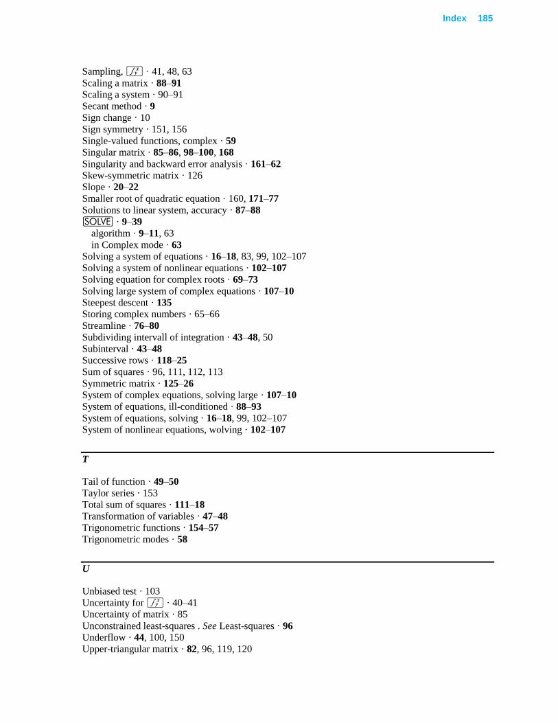
Index 185
Sampling, f · 41, 48, 63
Scaling a matrix · 88–91
Scaling a system · 90–91
Secant method · 9
Sign change · 10
Sign symmetry · 151, 156
Single-valued functions, complex · 59
Singular matrix · 85–86, 98–100, 168
Singularity and backward error analysis · 161–62
Skew-symmetric matrix · 126
Slope · 20–22
Smaller root of quadratic equation · 160, 171–77
Solutions to linear system, accuracy · 87–88
_ · 9–39
algorithm · 9–11, 63
in Complex mode · 63
Solving a system of equations · 16–18, 83, 99, 102–107
Solving a system of nonlinear equations · 102–107
Solving equation for complex roots · 69–73
Solving large system of complex equations · 107–10
Steepest descent · 135
Storing complex numbers · 65–66
Streamline · 76–80
Subdividing intervall of integration · 43–48, 50
Subinterval · 43–48
Successive rows · 118–25
Sum of squares · 96, 111, 112, 113
Symmetric matrix · 125–26
System of complex equations, solving large · 107–10
System of equations, ill-conditioned · 88–93
System of equations, solving · 16–18, 99, 102–107
System of nonlinear equations, wolving · 102–107
T
Tail of function · 49–50
Taylor series · 153
Total sum of squares · 111–18
Transformation of variables · 47–48
Trigonometric functions · 154–57
Trigonometric modes · 58
U
Unbiased test · 103
Uncertainty for f · 40–41
Uncertainty of matrix · 85
Unconstrained least-squares . See Least-squares · 96
Underflow · 44, 100, 150
Upper-triangular matrix · 82, 96, 119, 120

186 Index
186
V
Variables, transforming · 47–48
W
Weighted least-squares · 93–94, 97–98, 120
Weighted normal equations · 94
Y
Yield · 35
Z
Zero of polynomial · 13


![Abramowitz & Stegun - Handbook of Mathematical Functions [1970]](https://img.pdfslide.us/doc/110x75/54507e19b1af9fd07b8b4dee/abramowitz-stegun-handbook-of-mathematical-functions-1970.jpg)