Embed Size (px)
Citation preview

Please do not quote!
Advanced Econometrics 1
and
Theoretical Econometrics
Lecture Notes
Laszlo Matyas
2020
1
Topics : 1− 2
Short Introduction to Identificationand Asymptotics
2
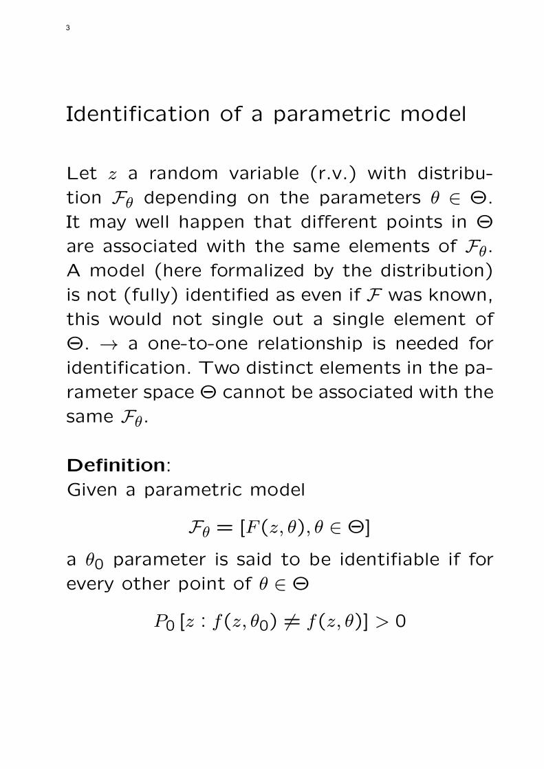
Identification of a parametric model
Let z a random variable (r.v.) with distribu-
tion Fθ depending on the parameters θ ∈ Θ.
It may well happen that different points in Θ
are associated with the same elements of Fθ.
A model (here formalized by the distribution)
is not (fully) identified as even if F was known,
this would not single out a single element of
Θ. → a one-to-one relationship is needed for
identification. Two distinct elements in the pa-
rameter space Θ cannot be associated with the
same Fθ.
Definition:
Given a parametric model
Fθ = [F (z, θ), θ ∈ Θ]
a θ0 parameter is said to be identifiable if for
every other point of θ ∈ Θ
P0 [z : f(z, θ0) = f(z, θ)] > 0
3

where P0 denotes the probability with respect
to the density f(z, θ0). A model is (fully) iden-
tified if it is identified in all its parameter points
∈ Θ.
Partial identification → identification in a re-
stricted parameter space. E.g., Local identifi-
cation → “around”, in the “neighbourhood” of
a parameter value.
Asymptotic identification → when the model is
identified in large samples (sample size → ∞).
EXAMPLE:
Let Fθ the parametric model generated by r.v.
u ∼ N2(0, I2) (2D normal r.v.) through the
transformation g(u) = Γu, where Γ is a (2×2)
matrix.
This model is NOT identified as, for example,
Γ0 =
(2 11 2
), Γ1 =
( √5 0
4/√5 3/
√5
)
4

are associated with the same N2(0, σ):
Σ = Γ0Γ′0 = Γ1Γ
′1 =
(5 44 5
).
Elements of asymptotic theory(Detailed theory in lecture READER 1!)
Definition: Limit of a deterministic sequence (or
convergnece)
Series xn, n = 1, . . . converges to a constant c
if for any ε > 0 there is an n ≥ N such that
|xn − c| < ε, then limn→∞xn = c .
Definition: Limit of a random sequence
Series of random variables xn converges to con-
stant c if
limn→∞Prob [(|xn − c|) > ε] = 0, for any ε > 0.
5
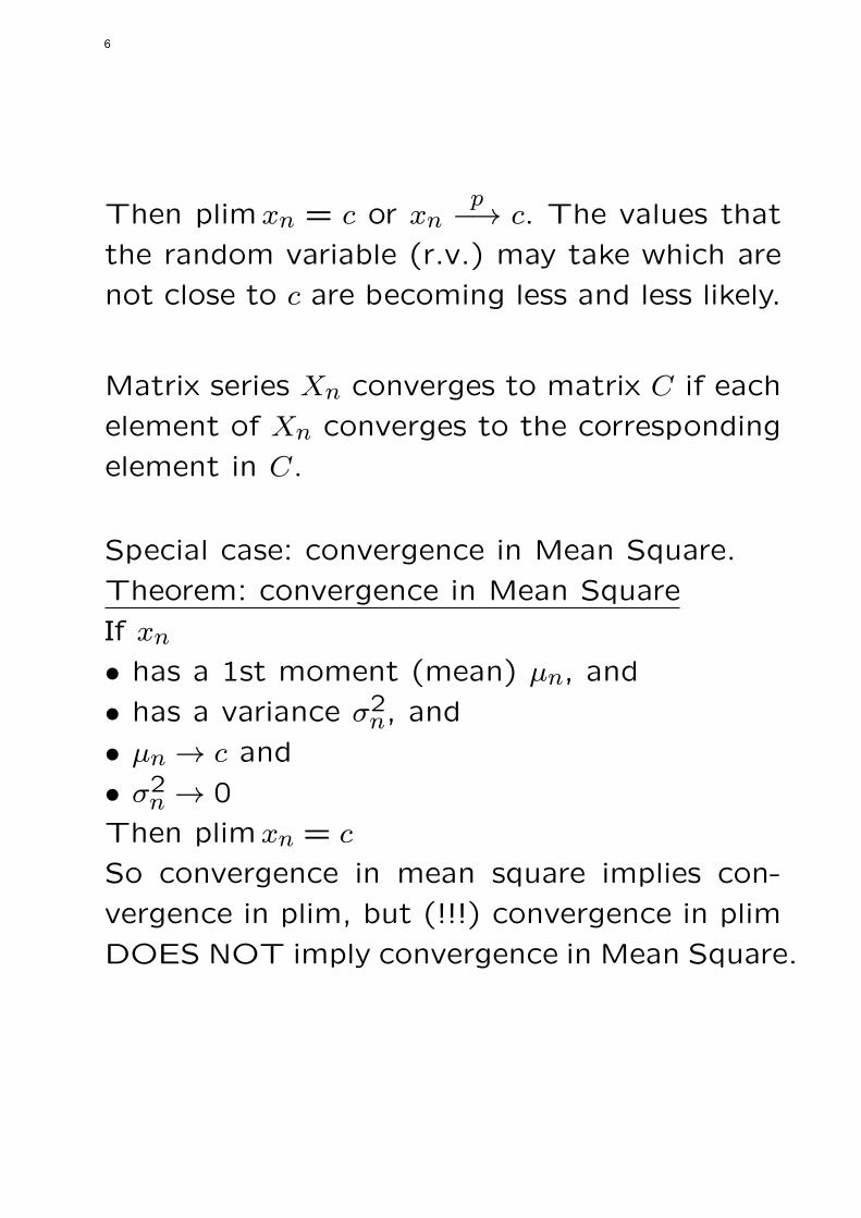
Then plimxn = c or xnp−→ c. The values that
the random variable (r.v.) may take which are
not close to c are becoming less and less likely.
Matrix series Xn converges to matrix C if each
element of Xn converges to the corresponding
element in C.
Special case: convergence in Mean Square.
Theorem: convergence in Mean Square
If xn
• has a 1st moment (mean) µn, and
• has a variance σ2n, and
• µn → c and
• σ2n → 0
Then plimxn = c
So convergence in mean square implies con-
vergence in plim, but (!!!) convergence in plim
DOES NOT imply convergence in Mean Square.
6

Slutsky theoremFor a continous function g(xn), which is not afunction of n
plim g(xn) = g(plimxn) .
Properties of the plim
If plimxn = c and plim yn = d, then:plim(xn + yn) = c+ d
plimxnyn = c d
plim xnyn
= cd, d = 0 .
If XN is an invertible random matrix,then plimXn = Ω implies plimX−1
n = Ω−1.
Uniform convergence in probabilitySeries of r.v. xn(θ) (r.v. x depends on θ) con-verges uniformly to the constant c(θ) in prob-ability on the parameter space Ω if
limn→∞P (sup
θ∈Ω|xn(θ)− c(θ)| < ξ) = 1 ∀ξ > 0
7

Some laws of large numbersGeneric Weak Law of Large Numbers - WLLN
Let xn be a series of r.v. on n = 1, . . . , N , with
E(xn) = µ If some regularity conditions are
met, then
xn =
∑Nn=1 xn
N
p−→ µ .
Some “applications” of this.
WLLN for iid series
Let xn be a series of r.v. on n = 1, . . . , N , with
E(xn) = µ and the same variance σ2 = E(xn−µ)2, then
xn =
∑xn
N
p−→ µ .
WLLN for non iid series
Let xn be a series of i.i.d. r.v. on n = 1, . . . , N ,
with E(xn) = µ and different variances σ2n =
E(xn − µ)2. If V ar(xn) → 0, then
xnp−→ µ .
8

Distributions
Definition: Convergence in distribution
Let xn series of r.v. with cdf Fn(x), then xn
converges in distribution to a r.v x with cdf
F (x) if
limn→∞ |Fn(x)− F (x)| = 0
at all points of F (x): xnd−→ x. This called the
Limiting Distribution.
Convergence in distribution DOES NOT mean
convergence in plim! Let us see an example!
Let r.v xn have the following distribution:
Prob(xn = 1) =1
2+
1
n+1
Prob(xn = 2) =1
2−
1
n+1
Now
xnd−→ f(x) =
P (x = 1) = 1/2
P (x = 2) = 1/2
9
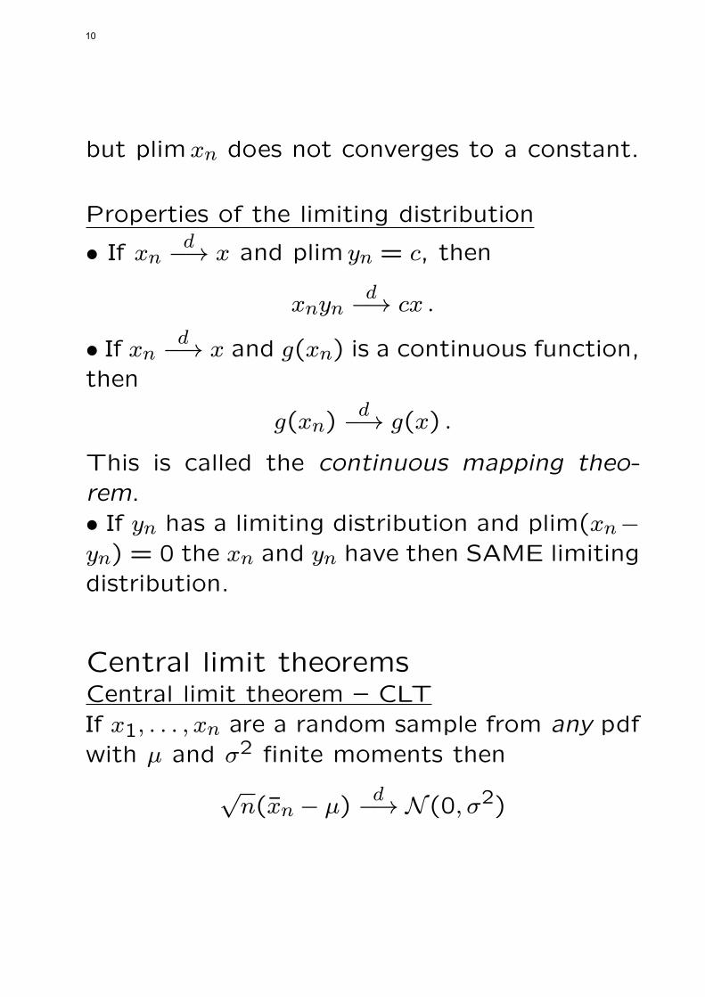
but plimxn does not converges to a constant.
Properties of the limiting distribution
• If xnd−→ x and plim yn = c, then
xnynd−→ cx .
• If xnd−→ x and g(xn) is a continuous function,
then
g(xn)d−→ g(x) .
This is called the continuous mapping theo-rem.• If yn has a limiting distribution and plim(xn−yn) = 0 the xn and yn have then SAME limitingdistribution.
Central limit theoremsCentral limit theorem – CLTIf x1, . . . , xn are a random sample from any pdfwith µ and σ2 finite moments then
√n(xn − µ)
d−→ N (0, σ2)
10

Lindberg – Levy CLTIf x1, . . . , xn are a random sample from a mul-tivariate distribution (random vectors) with fi-nite moment µ and Q covariance matrix, then
√n(xn − µ)
d−→ N (0, Q)
Lindberg – Feller CLTIf x1, . . . , xn are a random sample from a multi-variate distribution with finite moment E(xi) =µi, it’s demeaned version E(xi − µi) = 0 ∀i,V ar(xi) = Qi,
Qn =
∑iQi
n, lim Qn = Q pos. definite ∀n
and some regularity conditions are satisfied,then
√n(xn − µn)
d−→ N (0, Q)
with µn = 1n
∑i µi.
Definition: Asymptotic DistributionIt is a distribution to approximate the (often
11
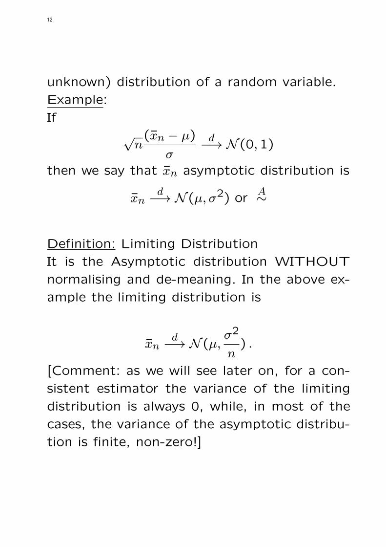
unknown) distribution of a random variable.
Example:
If√n(xn − µ)
σ
d−→ N (0,1)
then we say that xn asymptotic distribution is
xnd−→ N (µ, σ2) or
A∼
Definition: Limiting Distribution
It is the Asymptotic distribution WITHOUT
normalising and de-meaning. In the above ex-
ample the limiting distribution is
xnd−→ N (µ,
σ2
n) .
[Comment: as we will see later on, for a con-
sistent estimator the variance of the limiting
distribution is always 0, while, in most of the
cases, the variance of the asymptotic distribu-
tion is finite, non-zero!]
12

Rates of convergence – Order notation
Definition: Same Order
A deterministic sequence θT is O(T k) (of the
order T k) if: for some M > 0, there exists some
number K such that∣∣∣∣T−kθT
∣∣∣∣ < M
for all T > K.
This definition states that θT is O(T k) if T−kθTbecomes bounded as T → ∞. Notice it must
hold for some M , not all M . If the definition
held for all M then T−kθT would converge to
zero.
Example 1:
If
θT = T2,
then θT = O(T2) since T−2θT = 1 for all T ,
and hence is bounded for all T .
13

Example 2: (a bit more challenging)If
θT =T∑
t=1
t,
then θT = O(T2).
Definition: Smaller/Lower OrderA deterministic sequence θT is o(T k) if: forall ϵ > 0, there exists some number K suchthat ∣∣∣∣T−kθT
∣∣∣∣ < ϵ
for all T > K.That is, if θT = o(T k) then
T−kθT → 0.
This notation is used most commonly as “θT =op(1)”, to state that θT → 0.Example:
θT =T∑
t=1
t then θT = o(T3) .
14

Operations with orders:
O(np)±O(nq) = O(nmax(p,q))
o(np)± o(nq) = o(nmax(p,q))
O(np)± o(nq) = O(np) if p ≥ q
O(np)± o(nq) = o(nq) if p < q
O(np)O(nq) = O(n(p+q))
o(np)o(nq) = o(n(p+q))
O(np)o(nq) = o(n(p+q))
Example: xt has µ as a first moment, and the
CLT applies to it, then
n∑t=1
xt = O(n) if µ = 0
and in the de-meaned casen∑
t=1
(xt − µ) = O(n1/2) .
15

Applying asymptotics to the linear re-gression model
y = Xβ + u
and the “usual” assumptions apply. Further,
we also assume that
limn→∞
1
nX ′X = Q positive definite
then
plim βOLS = β +plim(1
nX ′X)−1 (
1
nX ′u)
= β +Q−1 plim(1
nX ′u)
From the Mean Square Convergence, we need
lim1
nX ′uu′X
1
n=
σ2
n
X ′X
n
limσ2/n = 0, limX ′X/n = 0
so plim 1nX
′u = 0, i.e., the OLS is consistent.
16

Now let us see the asymptotic distribution of
the OLS. We are interested in
√n(β − β) =
(X ′X
n
)−1 1√nX ′u
and we need the limiting distribution of 1√nX ′u.
Using the Lindberg–Feller CLT we get
1√nX ′u d−→ N (0, σ2Q)
which implies that
√n(β − β)
A∼ N (0, σ2Q−1) .
17

Topic : 3
Maximum Likelihood Estimation
18

Inverse Function
For scalars:
y = f(x)
where f(.) is strictly monotonic, there is aninverse function such as
x = f−1(y)
Example:
y = a+ bx
x = −a
b+
1
by
where
d x
d y=
d f−1(y)
d y
is the Jacobian of the transformation, here 1b .
For vectors:
y = f(x) , J =∂x
∂y′
19

is the Jacobian matrix,∂x1∂y1
. . . ∂x1∂yn... . . . . . .
∂xn∂y1
. . . ∂xn∂yn
Example:
y = Ax
x = A−1y
where abs(det(J)) i.e., the absolute value of thedeterminant is the Jacobian of x to y;
abs(det(J)) = abs(det(A−1)) =1
abs(det(A))
Let us now turn to the case of distributions.
Assume that x1 and x2 are random variableswith a joint distribution fx(x1, x2) and y1 andy2 are two monotonic functions of x1 and x2:
y1 = y1(x1, x2)
y2 = y2(x1, x2)
20
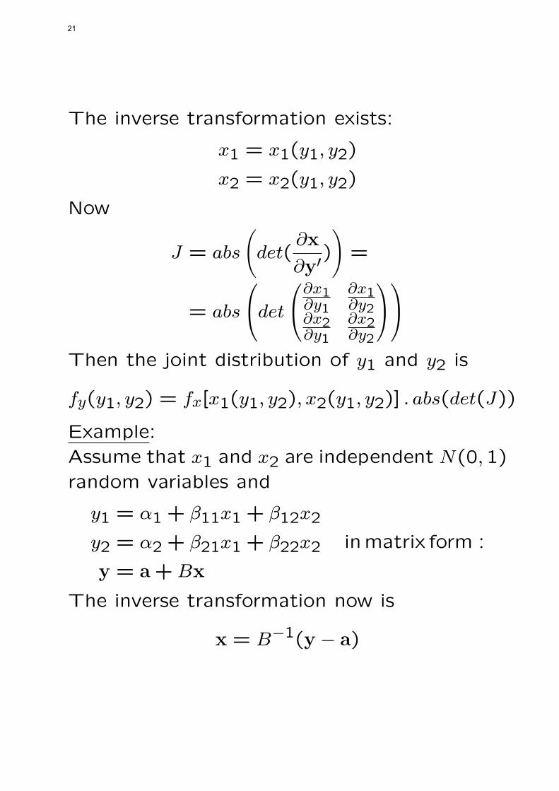
The inverse transformation exists:
x1 = x1(y1, y2)
x2 = x2(y1, y2)
Now
J = abs
(det(
∂x
∂y′)
)=
= abs
det∂x1
∂y1∂x1∂y2
∂x2∂y1
∂x2∂y2
Then the joint distribution of y1 and y2 is
fy(y1, y2) = fx[x1(y1, y2), x2(y1, y2)] . abs(det(J))
Example:
Assume that x1 and x2 are independent N(0,1)
random variables and
y1 = α1 + β11x1 + β12x2
y2 = α2 + β21x1 + β22x2 inmatrix form :
y = a+Bx
The inverse transformation now is
x = B−1(y − a)
21

and the Jacobian
J = abs(det(B−1)
)=
1
abs (det(B))
The joint distribution of x is the product of
the marginals since they are assumed to be
independent:
fx(x) = (2π)−1e−(x21+x22)/2
= (2π)−1e−X ′X/2
and so
fy(y) = (2π)−1 1
abs(det(B))e−((y−a)′(BB′)−1(y−a))/2
In general: If x is a continuous r.v. with pdf
fx(x) and y = g(x) is an invertible function of
x then the density of y is
fy(y) = fx(g−1(y)).abs
(det(d g−1(y))
)where d stands for the first derivative.
22

Example:
Let be
x ∼ N(0, I) y = A′x+ µ
y ∼ N(µ, V ), V = A′A
The Jacobian from y to x is now abs(det(A−1)).
The density of y in then
y = (2π)−n/2abs(det(A)−1
)×
× exp[−1/2(y − µ)′A−1A−1′(y − µ)]
= (2π)−n/2abs(det(V )−1/2
)×
× exp[−1/2(y − µ)′V −1(y − µ)]
Likelihood estimation
Reminder: Analytically the joint density func-
tion and the likelihood function are the same.
The difference is in how we look at it. In the
density function the parameters are known and
the variables are unknown. In the likelihood
23
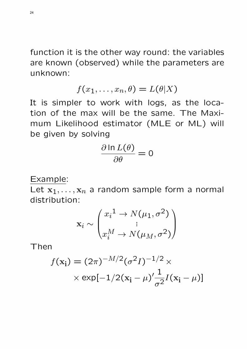
function it is the other way round: the variablesare known (observed) while the parameters areunknown:
f(x1, . . . , xn, θ) = L(θ|X)
It is simpler to work with logs, as the loca-tion of the max will be the same. The Maxi-mum Likelihood estimator (MLE or ML) willbe given by solving
∂ lnL(θ)
∂θ= 0
Example:Let x1, . . . ,xn a random sample form a normaldistribution:
xi ∼
xi1 → N(µ1, σ
2)...
xMi → N(µM , σ2)
Then
f(xi) = (2π)−M/2(σ2I)−1/2×
× exp[−1/2(xi − µ)′1
σ2I(xi − µ)]
24

Now taking the logs and summing over the
sample gives
lnL = −nM
2ln(2π)−
nM
2lnσ2−
−1
2σ2∑i
(xi − µ)′(xi − µ)
For the MLE
∂ lnL
∂µ=
1
σ2
∑i
(xi − µ)
∂ lnL
∂σ2= −
nM
2σ2+
1
2σ4∑i
(xi − µ)′(xi − µ)
Solving these equations gives:
µMLE,m = xm =1
n
∑i
xi,m
σ2 =
∑i∑
m(xim − xm)2
nM
ML estimation of the linear regressionmodel
25

y = Xβ + u
L(β, σ2|y, X) → L(β, σ2) → L
= (2πσ2)−n/2 exp[−(y −Xβ)′(y −Xβ)/2σ2]
The log-likelihood is
lnL = −n/2 ln(2π)− (n/2) lnσ2
− (y −Xβ)′(y −Xβ)/2σ2
To maximise it:
∂L
∂β=
1
σ2X ′(y −Xβ) = 0
∂L
∂σ2= −
n
2σ2+
(y −Xβ)′(y −Xβ)
2σ4= 0
Solving this gives
βML = (X ′X)−1X ′y
σ2ML = (y −XβML)′(y −XβML)/n
In most of the cases maximising the likelihooddoes not give a closed analytical form. Often tocarry out the max one needs numerical tools.
26
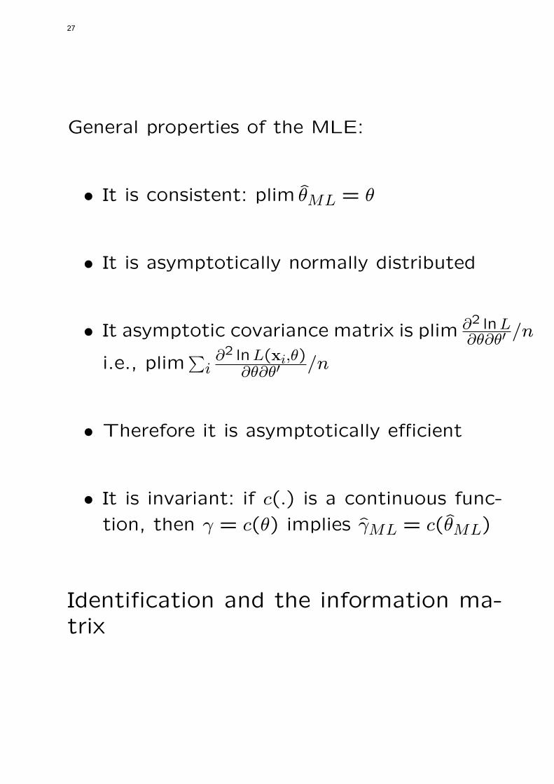
General properties of the MLE:
• It is consistent: plim θML = θ
• It is asymptotically normally distributed
• It asymptotic covariance matrix is plim ∂2 lnL∂θ∂θ′ /n
i.e., plim∑
i∂2 lnL(xi,θ)
∂θ∂θ′ /n
• Therefore it is asymptotically efficient
• It is invariant: if c(.) is a continuous func-
tion, then γ = c(θ) implies γML = c(θML)
Identification and the information ma-trix
27
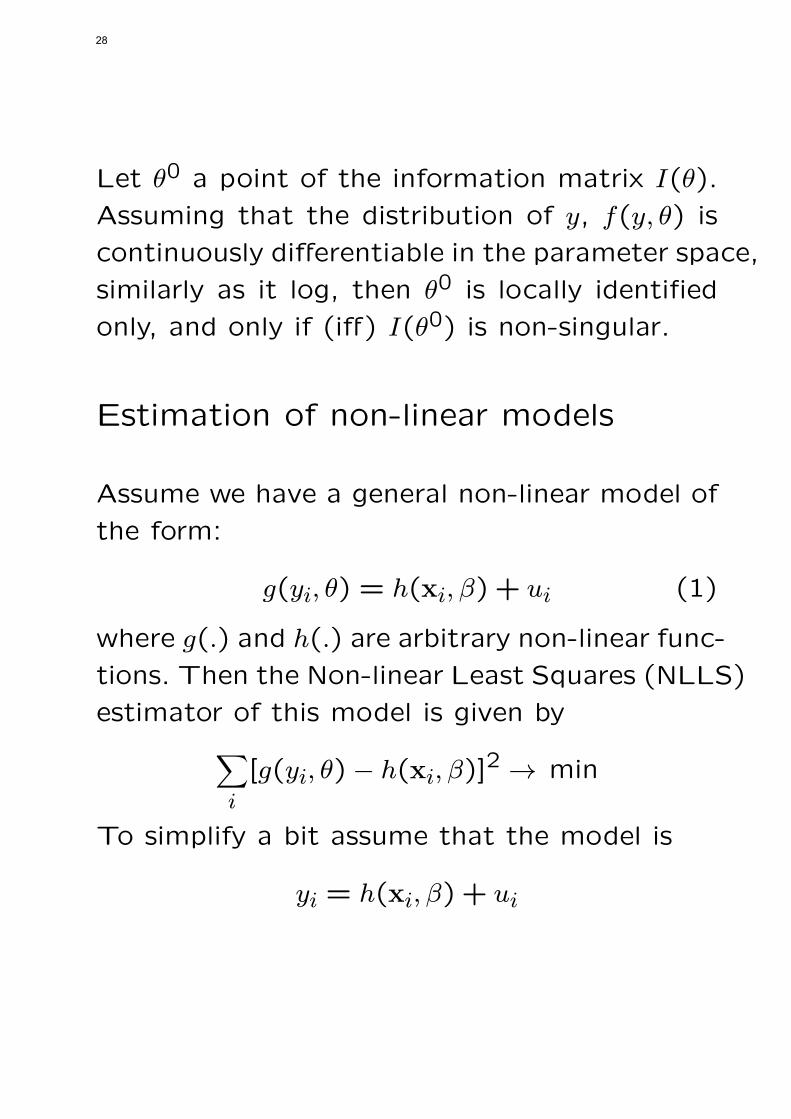
Let θ0 a point of the information matrix I(θ).
Assuming that the distribution of y, f(y, θ) is
continuously differentiable in the parameter space,
similarly as it log, then θ0 is locally identified
only, and only if (iff) I(θ0) is non-singular.
Estimation of non-linear models
Assume we have a general non-linear model of
the form:
g(yi, θ) = h(xi, β) + ui (1)
where g(.) and h(.) are arbitrary non-linear func-
tions. Then the Non-linear Least Squares (NLLS)
estimator of this model is given by∑i
[g(yi, θ)− h(xi, β)]2 → min
To simplify a bit assume that the model is
yi = h(xi, β) + ui
28
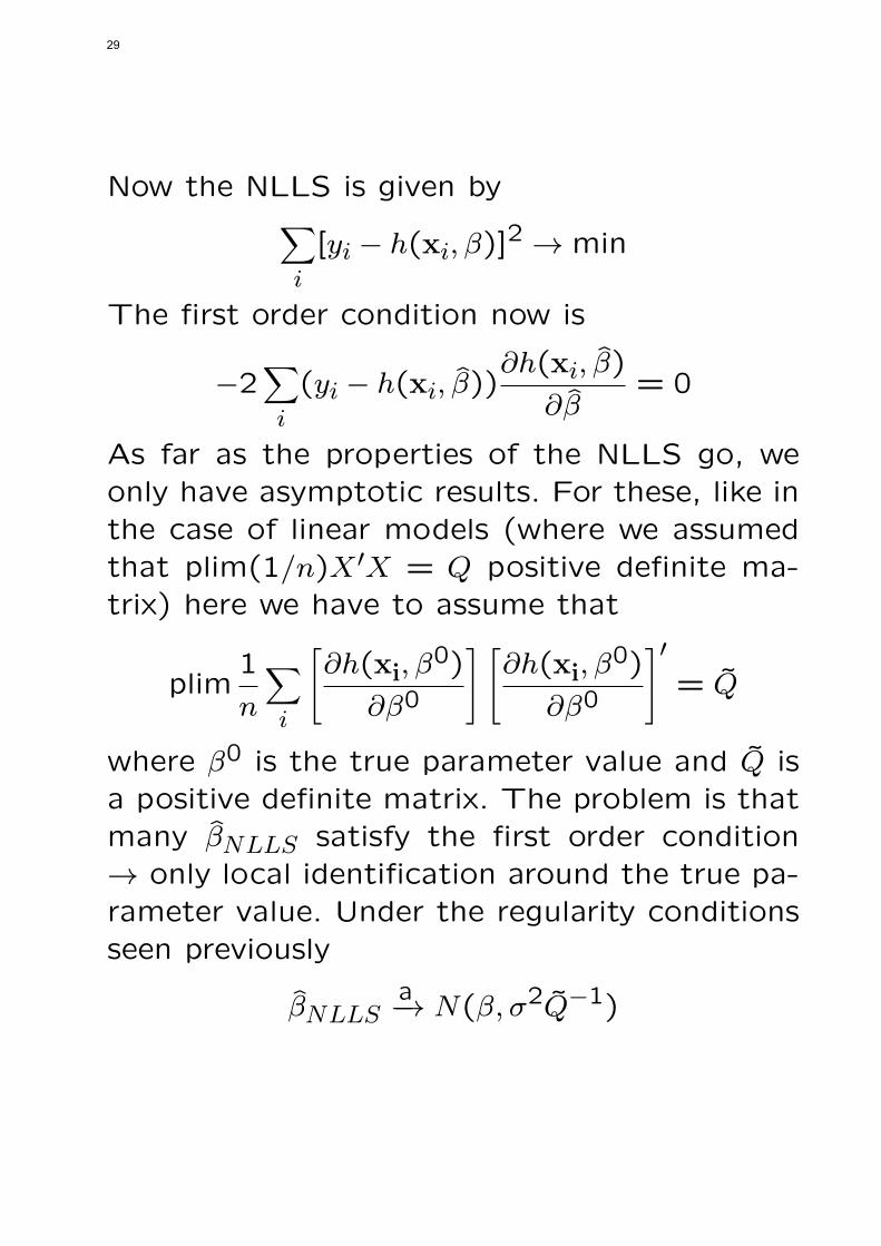
Now the NLLS is given by∑i
[yi − h(xi, β)]2 → min
The first order condition now is
−2∑i
(yi − h(xi, β))∂h(xi, β)
∂β= 0
As far as the properties of the NLLS go, weonly have asymptotic results. For these, like inthe case of linear models (where we assumedthat plim(1/n)X ′X = Q positive definite ma-trix) here we have to assume that
plim1
n
∑i
[∂h(xi, β
0)
∂β0
] [∂h(xi, β
0)
∂β0
]′= Q
where β0 is the true parameter value and Q isa positive definite matrix. The problem is thatmany βNLLS satisfy the first order condition→ only local identification around the true pa-rameter value. Under the regularity conditionsseen previously
βNLLSa−→ N(β, σ2Q−1)
29

Let us now turn back to the MLE and model(1). Assuming that the ui disturbance termsare normally distributed, the Jacobian is
J(yi, θ) = Ji = abs
(det(
∂g(yi, θ)
∂yi)
)so the log-likelihood is
lnL = −n/2 ln(2π)− n/2 lnσ2 +∑i
ln J(yi, θ)−
−1
2σ2∑i
[g(yi, θ)− h(xi, β)]2
The first order conditions are
∂ lnL
∂β= 1/σ2
∑i
ui∂h(xi, β)
∂β= 0
∂ lnL
∂θ=∑i
1
Ji(∂Ji∂θ
)− 1/σ2∑i
ui∂g(yi, θ)
∂θ= 0
∂ lnL
∂σ2= −
n
2σ2+
1
2σ4∑i
u2i = 0
(2)
In general numerical procedures are required tosolve it and to maximise the likelihood func-tion.
30

Concentrated likelihood
Many problems can be formulated by parti-
tioning the parameter vector θ = [θ1θ2] such
that the maximisation problem for θ2,ML can
be written as a function of θ1,ML:
θ2,ML = f(θ1,ML)
Then the concentrate likelihood is
Lc((θ1, θ2) = Lc(θ1, f(θ1))
Example 1:
From (2)
σ2ML = 1/n∑i
[g(yiθML)− h(xiβML)]2
Substituting this back into the lnL gives
lnLc =∑i
ln J(yi, θ)− n/2(1 + ln(2π))
− n/2 ln[1/n∑i
u2i ]
31

This concentrated log-likelihood is only a func-
tion of θ and β but not of σ2.
Example 2:
Estimation of the first two moments of a nor-
mal population:
lnL(µ, σ2) = −n
2[ln(2π) + lnσ2]−
−1
2σ2∑i
(xi − µ)2 which gives
σ2ML =1
n
∑i
(xi − µML)2
Now putting this back into the log-likelihood
we get
lnLc = −n
2
1+ ln(2π) + ln[1
n
∑i
(xi − µML)2]
The solution now for µ now is x. We can also
concentrate the log-likelihood over µ instead
of σ2.
32

Topic : 4
Pseudo Maximum Likelihood andExtremum Estimation
33

Pseudo (Quasi) Maximum Likelihood
The Kullbac–Leibler index/measure of prox-
imity/discrepancy measures the similarity be-
tween two distributions/densities. Let p(y) and
π(y) be two probability distributions for the
random variable Y . The KL index is:
KL(p, π) = Ep[ln(p(y)/π(y))]
where Ep[.] denotes the expectation taken with
respect to the density p(y).
The closer KL(p, π) to zero the more similar is
p(y) to πy. KL= 0 iff p(y) = π(y). If Ep[.] does
not exist, we take KL= ∞.
Application of the KL
Let us have the density f(z, θ0) and any other
density f(z, θ). Then
KL = E0[ln f(z, θ0)]− E0[ln f(z, θ)]
34

This means that searching for the maximumof the log-likelihood is in fact searching for theminimum KL!
Now let us turn to the Pseudo (Quasi) ML.Let us assume that the true pdf behind ourmodel is p(y) but our estimation, the pseudolikelihood, is based on the π(y, θ) pdf θ ∈ Ω. Letθ∗ be the value (called pseudo-true value)thatminimises the KL p(y) relative to π(y, θ):
θ∗ = minθ∈Ω
[Ep(ln(p(y)/π(y, θ))]
and pseudo/quasi ML based on the π(y, θ)
θQML → maxθ∈Ω
[lnLQ(θ, y, x)]
θQML consistently estimates θ∗ and it can beshow easily that
θQMLA∼ N(0, h(θ∗)−1Σ∗h(θ∗)−1]
where
Σ∗ =1
n
(∂ lnLQ(θ, y,X)
∂θ|θ∗
)(∂ lnLQ(θ, y,X)
∂θ|θ∗
)
35

and
h(θ∗) =1
n
(∂2 lnLQ(...)
∂θ∂θ′
)The main question now is how far the pseudo-
true value θ∗ is from the true value θ0?
Let us consider the “usual” model
yi = h(x,β0) + ui
with no endogeneity. Then, under the usual
regularity conditions (to be seen later on):
Theorem
The Pseudo (Quasi) ML estimator is “fully”
consistent (i.e., it is a consistent estimator of
the true parameter value θ0) if the pseudo-
likelihood is based on the exponential family
of distributions:
f(x, θ) = exp [A(θ).B(x) + C(x) +D(θ)]
36

where A(.), B(.), C9.) and D(.) are real val-ued functions. Examples of such distributions:Normal, Gamma, Binomial, Poisson, Geomet-ric, etc....
Extremum Estimation (or M-estimation)
Any estimator that can be written in the form
θ = argmaxθ∈Ω[m(θ, y,X)]
where m(.) is the objective function is an Ex-tremum Estimator (EE) also called M-estimator.The properties of the EE depends on someregularity conditions.
Examples
ML → m(θ, y,X) = L(θ, y,X)
OLS → m(θ, yX) = (y −Xβ)′(y −Xβ)
Asymptotic Properties
37

Consistency
Intuition: The criterion function m(.) converges
to a non-stochastic function of θ that is max-
imised uniquely at the true parameter value θ0if the limit of the max of m(.) = the max of
the limit of m(.), then the max of the objective
function converges to the max of m0(θ) which
is θ0.
Two sufficient (but not necessary) conditions
for the consistency of the EE (plim θ = θ0):
Theorem 1
a) m(θ, y,X) converges uniformly in probabil-
ity to a function of θ, say m0(θ),
[m(, θ, ...)p−→ m0(θ)]
b) m0(θ) is continuous in θ
38

c) m0(θ) is uniquely maximised at θ
d) The parameter space Ω is compact (closed
and bounded)
Theorem 2
a)-c) a) and c) the same as above
b) m0(θ) is concave in θ
d) Ω is a convex set with θ0 inside
Asymptotic normality
Intuition: EE is an asymptotically linear func-
tion of a multivariate normal r.v. so it is itself
as. normally distributed.
39

Theorem 3: Conditions for the asymptotic nor-
mality
a) plim(θ) = θ0
b) θ0 is inside Ω
c) m(.) is twice continuously differentiable in
θ in the neighborhood (κ(θ0)) of θ0
d)
√n∂m(θ, y,X)
∂θ|θ0
d−→ N(0,Σ)
e)
limn→∞P
supθ∈κ(θ)
||∂2m(...)
∂θ∂θ′− h(θ)|| < ε
= 1
∀ε > 0
40

where h(θ) is a function and ||...|| is the Eu-
clidean distance from zero, if C is a matrix
→ [vec(C)′vec(C)]1/2
f) h(θ) is continuous and non-singular at θ0
Then√n(θ − θ0)
d−→ N(0, h(θ0)
−1Σh(θ0)−1)
Application
The ML estimator is consistent if
a) 1/n lnL(θ) converges uniformly in proba-
bility to L0(θ)
b) L0(θ) is continuous in θ
c) L0(θ) is uniquely maximised at θ0
41

d) Ω is compact
The ML estimator has an asymptotic normal
distribution if
a) θp−→ θ0
b) θ0 is inside Ω
c) 1/n lnL(θ) is twice differentiable
d)
(1/√n)
∂ lnL(...)
∂θ|θ0
d−→ N(0,Σ)
e)
1/n∂2 lnL(...)
∂θ∂θ′
42

converges in probability to h(θ)
f) The same as in Theorem 3
43

Topic : 6
Elements of Hypothesis Testing inEconometrics
44

Hypothesis testing
Hypothesis testing is based on a test-function
(or test statistic) with known distribution un-
der the H0 hypothesis.
Type I error → when we reject the null hypoth-
esis when in fact it is true.
Type II error → when we do not reject the null
hypothesis when in fact it is not true.
Significance level of a test (1%,5%,10%) is
the probability of Type I error. This is also
called the size of the test.
The power of a test is 1− the probability of
Type II error: 1− Prob(Type II error).
Uniformly Most Powerful (UMP) test has greater
power than any other test of the same size for
all admissible values of the parameter(s).
Unbiased test: It has greater power than size
for all admissible parameter values (quite weak
45

requirement!). If a test is biased for some pa-
rameter values we are more likely to accept the
null when it is false than when it is true.
Consistent test: Power → 1 as n → ∞.
Some important types of tests
Simple/composite hypotheses: A hypothesis that
completely specifies the distribution of the r.v
Z (the test statistic) is called simple, otherwise
it is composite. Example → simple: H0 : θ = θ0;
composite H1 : θ = θ0.
Nested hypotheses: When the Ωθ parameter
space is made up of two disjoint subsets Ωθ0and Ωθ1 with Ωθ1 = Ωθ − Ωθ0 the H0 related
on Ωθ0 is nested in HA related to Ωθ.
When both the null and the alternative hy-
potheses are simple (e.g., H0 : θ = θ0 and
46

HA : θ = θ1 then the Neyman-Pearson theo-
rem guarantees the existence of a UMP test.
On the other hand, when the alternative is
composite there is a UMP test only iff the crit-
ical region is the same for each simple alter-
natives that make up HA. → This is a very
exceptional case, in practice does not happen.
Testing for parameter restrictions
Consider the ML estimation of the parame-
ter(s) θ and test
H0 : C(θ) = 0
where C(.) are a set of restrictions on the pa-
rameter(s).
1. The Likelihood Ratio (LR) test
Intuition: If the restrictions C(θ) are valid
(true) in the sample, imposing them for
47
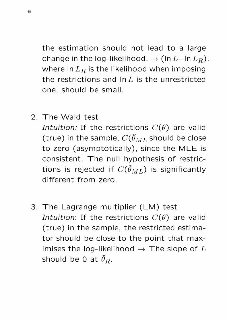
the estimation should not lead to a large
change in the log-likelihood. → (lnL−lnLR),
where lnLR is the likelihood when imposing
the restrictions and lnL is the unrestricted
one, should be small.
2. The Wald test
Intuition: If the restrictions C(θ) are valid
(true) in the sample, C(θML should be close
to zero (asymptotically), since the MLE is
consistent. The null hypothesis of restric-
tions is rejected if C(θML) is significantly
different from zero.
3. The Lagrange multiplier (LM) test
Intuition: If the restrictions C(θ) are valid
(true) in the sample, the restricted estima-
tor should be close to the point that max-
imises the log-likelihood → The slope of L
should be 0 at θR.
48

1. The LR test:
λ =L(θ)RL(θ)
0 < λ < 1
If λ is too small the restriction are probably not
true. Under the usual regularity conditions
−2 lnλA∼ χ2
with DF equal to the number of restrictions.
2. The Wald test.
To deal with this we need a technical detour!
Full rank quadratic form. If
u ∼ N(µ,Σ)
then
Σ−1/2(u− µ) ∼ N(0, I)
and
(u− µ)′Σ−1(u− µ) ∼ χ2(n)
Now if the H0 hypothesis that E(u) = µ is true,
this will have a χ2 distribution, if false the form
49

will likely to be large.
Let us go now back to the Wald test and the
θ be the unrestricted parameter estimate.
H0 : C(θ) = q
If true (C(θ)− q) should be close to zero.
W =[(C(θ)− q)′(V ar(C(θ − q))−1(C(θ)− q)
]A∼ χ2
if the null is true, with DF equal to the number
of restrictions, i.e., the number of equations in
(C(θ)− q))
Let us have a small detour again!
if√n(θ − θ)
d−→ N(0, σ2)
and g(θ) is a continuous function then
g(θ)d−→ N
(g(θ),plim(
g′(θ)2σ2
n)
)
50
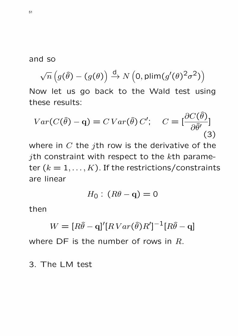
and so
√n(g(θ)− (g(θ)
) d−→ N(0,plim(g′(θ)2σ2)
)Now let us go back to the Wald test using
these results:
V ar(C(θ)− q) = C V ar(θ)C′; C = [∂C(θ)
∂θ′]
(3)
where in C the jth row is the derivative of the
jth constraint with respect to the kth parame-
ter (k = 1, . . . ,K). If the restrictions/constraints
are linear
H0 : (Rθ − q) = 0
then
W = [Rθ − q]′[RV ar(θ)R′]−1[Rθ − q]
where DF is the number of rows in R.
3. The LM test
51

The Lagrangian formulation:
maxθ
f(θ, . . . ) subject to
C1(θ) = 0...
CJ(θ) = 0
constraints is the same as
maxθ,λ
L∗(θ, λ) = f(θ) + λ′C(θ)
where L∗ is the Lagrangian and has a ∗ in ordernot to confused with the likelihood. First orderconditions are
∂L∗
∂θ=
∂f(θ)
∂θ+
∂λ′C(θ)
∂θ= 0
∂L∗
∂λ= C(θ) = 0 with
∂λ′C(θ)
∂θ= λ′C = C′λ
with C defined in (3). If the restriction aretrue/valid imposing them will have little effecton the estimation so λ is going to be small:
H0 : λ = 0
52

We know that
∂ lnL(θR)
∂θR≈ 0
I.e., the derivatives of the log-likelihood evalu-
ated at the restricted parameters will be ≈ 0.
This is also called the score test as
∂ lnL(θ)
∂θ
is the score. So similarly to the case of the
Wald test, the test statistic now is
LM =
(∂ lnL(θR)
∂θR
)′[I(θR)]
−1(∂ lnL(θR)
∂θR
)A∼ χ2
with DF equal to the number of restrictions.(The
variance of the first derivative vector here is the
Information matrix!)
In finite samples:
W ≥ LR ≥ LM
53

Asymptotically:
W = LR = LM
EXAMPLE 1
Let be a random sample x1, . . . , xn from a nor-
mal distribution with 1st moment µ and σ2 =
4. The H0 : µ = 2. For the LR test
maxLR =(1/2√2π)n exp[−1/8
∑i
(xi − 2)2] = LR
maxL =(1/2√2π)n exp[−1/8
∑i
(xi − x)2] = L
λ = exp[−1/8∑i
(xi − 2)2 +1/8∑i
(xi − x)2] =
= exp[−n/8(x− 2)2 so
LR = −2 lnλ =(x− 2)2
4/n∼ χ2(1) under H0
54

Now turning to the Wald test
W = (µML − 2)′V ar(µML)(µML − 2) with
V ar(µML) = E(∂2 lnL(µ)
∂µ2) = (
n
4) so
W = (x− 2)2(n
4)
And finally the LM (score) test. The score nowis
s(µ) =∂ lnL(µ)
∂µ=
=
∑i(xi − µ)
4= n
(x− µ)
4so under H0
s(2) =n(x− µ)
4and the LM
LM =n2(x− 2)2
16
4
n=
n(x− 2)2
4
EXAMPLE 2The same as above, but now the sample is
55

from a N(µ, σ2) distribution.
LR = N2 ln
∑i(xi − 2)2∑i(xi − x)2
W =N2(x− 2)2∑
i(xi − x)2
LM =N2(x− 2)2∑
i(xi − 2)2
56

Topic : 7
Instrumental Variables Estimation
57

IV estimation
The consistency of the LS methods rely on
plim1
TX ′u = 0 (4)
i.e., that all explanatory variables are indepen-
dent from (orthogonal to) the disturbance terms.
This condition cannot directly be verified as
by construction uLS residual is always uncorre-
lated with u → LS will not provide evidence of
the inconsistency. When this condition is not
satisfied, we talk about endogeneity.
Examples
Examples when this (4) condition is not satis-
fied.
1. Simple measurement error.
Let us have the simple relationship
yt = β0 + β1xt + ut
58

but only
x∗i = xi + vi
is observed where vi is a white noise. So in fact
we estimate the model
yi = β0 + β1x∗i − β1vi + ui︸ ︷︷ ︸
u∗i
with u∗i being the new disturbance term. Clearly
now x∗ and u∗ are correlated as there is a neg-
ative correlation.
2. Autocorrelation in the disturbances and lagged
dependent variable(s) in the model.
Let us have the model
yt = β0 + β1xt + β2yt−1 + εt
with εt = ρεt−1 + vt, where vt is a white noise
and ρ < 1, β2 < 1. Then
E(xtεt) = 0 but now
E(yt−1εt) = 0
59
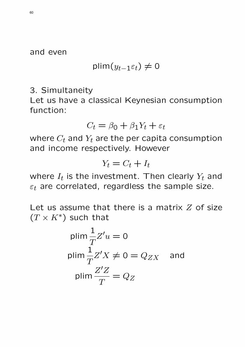
and even
plim(yt−1εt) = 0
3. SimultaneityLet us have a classical Keynesian consumptionfunction:
Ct = β0 + β1Yt + εt
where Ct and Yt are the per capita consumptionand income respectively. However
Yt = Ct + It
where It is the investment. Then clearly Yt andεt are correlated, regardless the sample size.
Let us assume that there is a matrix Z of size(T ×K∗) such that
plim1
TZ′u = 0
plim1
TZ′X = 0 = QZX and
plimZ′Z
T= QZ
60
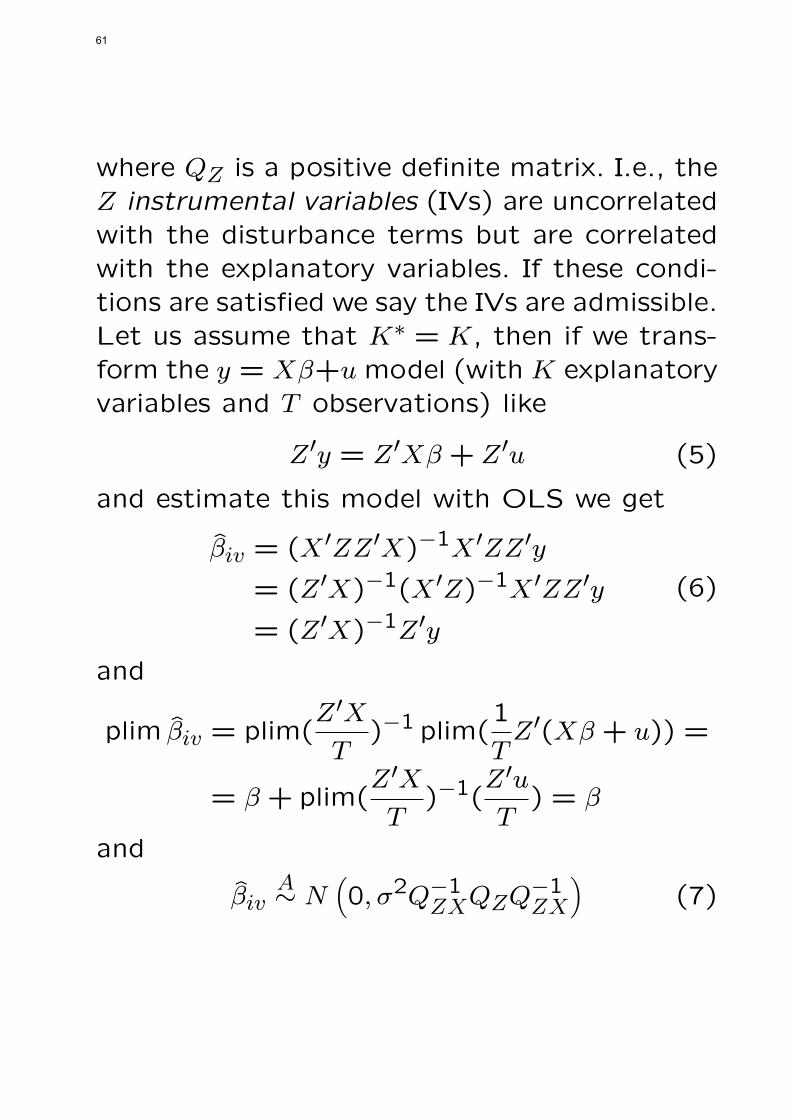
where QZ is a positive definite matrix. I.e., theZ instrumental variables (IVs) are uncorrelatedwith the disturbance terms but are correlatedwith the explanatory variables. If these condi-tions are satisfied we say the IVs are admissible.Let us assume that K∗ = K, then if we trans-form the y = Xβ+u model (with K explanatoryvariables and T observations) like
Z′y = Z′Xβ + Z′u (5)
and estimate this model with OLS we get
βiv = (X ′ZZ′X)−1X ′ZZ′y
= (Z′X)−1(X ′Z)−1X ′ZZ′y
= (Z′X)−1Z′y
(6)
and
plim βiv = plim(Z′X
T)−1 plim(
1
TZ′(Xβ + u)) =
= β +plim(Z′X
T)−1(
Z′u
T) = β
and
βivA∼ N
(0, σ2Q−1
ZXQZQ−1ZX
)(7)
61

The number of IVs can be larger than the num-
ber of (stochastic) explanatory variables (that
need to be instrumented for). For the non-
stochastic explanatory variables the instruments
are themselves. (But the number of IVs must
be < T .) Next let us assume that K∗ > K.
Then the transformed model (5) should be es-
timated by GLS instead of OLS. This gives
βiv = [X ′Z(Z′Z)−1Z′X]−1[X ′Z(Z′Z)−1Z′]y(8)
When K∗ = K this gives back estimator (6).
The asymptotic covariance matrix of this es-
timator is also (7). When X and Z are not
strongly correlated the standard errors based
on (7) can be very large. → in this case we
talk about weak instruments.
For this estimator (8) in fact we minimise the
quadratic form
(y −Xβ)PZ(y −Xβ) where
PZ = Z(Z′Z)−1Z′
62

So far we have implicitly assumed that the dis-
turbance term of the untransformed model u
has a scalar covariance matrix, i.e., E(uu′) =
σ2I. When this is not the case and E(uu′) = Ω
the covariance matrix of model (5) is (Z′ΩZ).
Therefore the GLS estimator becomes
βiv = [X ′Z(Z′ΩZ)−1Z′X]−1×× [X ′Z(Z′ΩZ)−1Z′]y
with asymptotic covariance matrix
σ2
Q−1ZX plim(
Z′ΩZ
T
−1
)Q−1ZX
If K∗ = K this gives back (6). Now let us look
at another type of IV estimator. Let us call it
“GLS analog” IV. We know that a covariance
matrix Ω can be decomposed as
P ∗ΩP ∗ = IT and P ∗′P ∗ = Ω−1
First let us transform the model as
P ∗y = P ∗Xβ + P ∗u︸ ︷︷ ︸Scalar cov.matrix
63

So if we transform with P ∗ the instruments as
well and then instrument this model we get
Z′P ∗′P ∗y = Z′P ∗′P ∗Xβ + Z′P ∗′P ∗u
Z′Ω−1y = Z′Ω−1Xβ + Z′Ω−1u leading to
βiv = [X ′Ω−1Z(Z′Ω−1Z)−1Z′Ω−1X]−1×× [X ′Ω−1Z(Z′Ω−1Z)−1Z′Ω−1]y
Why is this “GLS analog”? Because if we have
K∗ = K we get back a GLS type estimator:
βiv = (Z′Ω−1X)−1Z′Ω−1y
The orthogonality condition needed for consis-
tency is
plim1
TZ′Ω−1u = 0
Non-linear IVLet be the general non-linear model
yi = g(xi, β) + ϵi
64
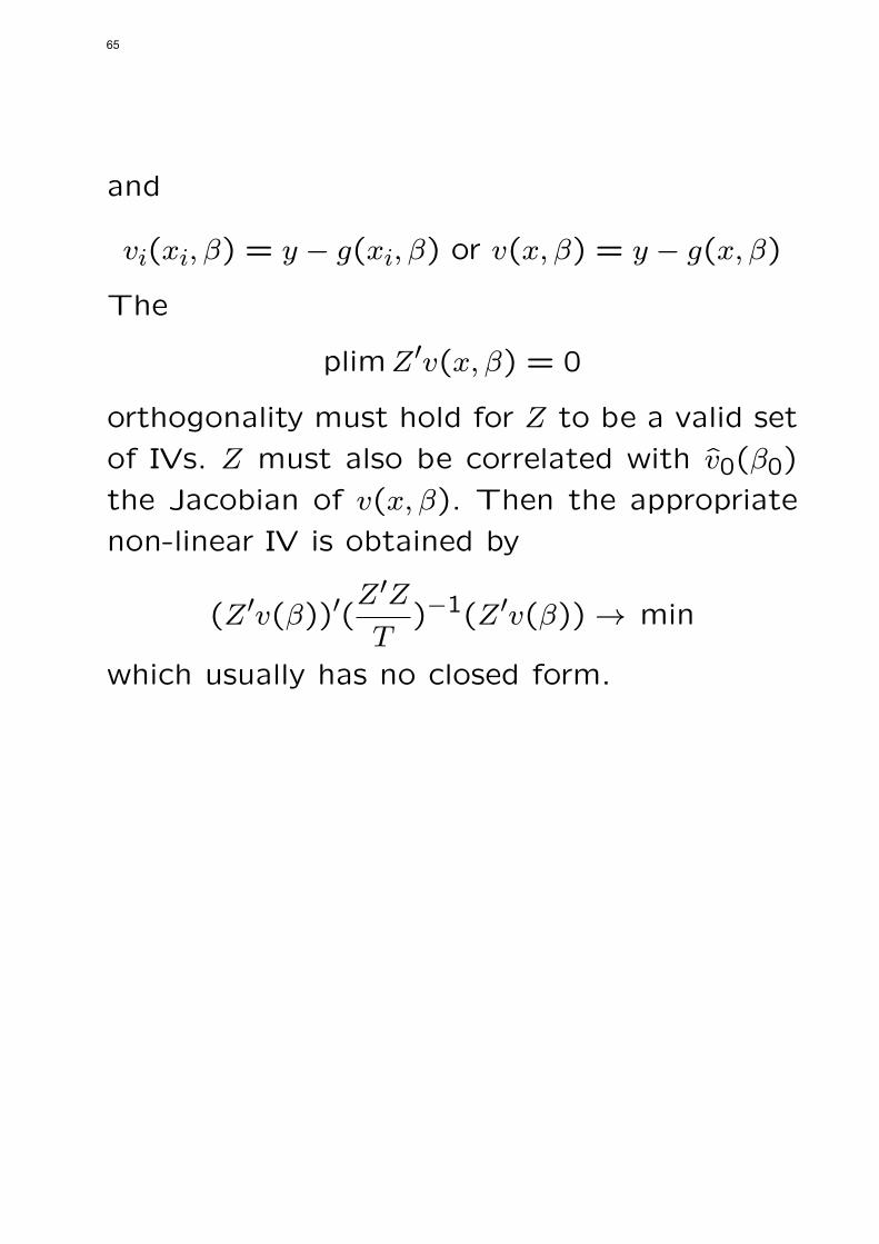
and
vi(xi, β) = y − g(xi, β) or v(x, β) = y − g(x, β)
The
plimZ′v(x, β) = 0
orthogonality must hold for Z to be a valid set
of IVs. Z must also be correlated with v0(β0)
the Jacobian of v(x, β). Then the appropriate
non-linear IV is obtained by
(Z′v(β))′(Z′Z
T)−1(Z′v(β)) → min
which usually has no closed form.
65

Topic : 8
Generalised Method of MomentsEstimation – GMM
66

GMM estimation
One of the most important tasks in econo-
metrics and statistics is to find techniques en-
abling us to estimate, for a given data set,
the unknown parameters of a specific model.
Estimation procedures based on the minimi-
sation (or maximisation) of some kind of cri-
terium function (EE or M–estimators) have
successfully been used for many different types
of models. The main difference between these
estimators lies in what must be specified of
the model. The most widely applied such esti-
mation, the maximum likelihood, requires the
complete specification of the model and its
probability distribution. The Generalised Method
of Moments (GMM) does not require this sort
of full knowledge. It only demands the speci-
fication of a set of moment conditions which
the model should satisfy.
67

Let us start with the Method of Moments (MM)
estimation.
The Method of Moments – MM
The Method of Moments is an estimation tech-
nique which suggests that the unknown param-
eters should be estimated by matching popula-
tion (or theoretical) moments (which are func-
tions of the unknown parameters) with the ap-
propriate sample moments. The first step is to
properly define the moment conditions.
Moment Conditions
Assume that we have a sample xt : t = 1, . . . , Tfrom which we want to estimate an unknown
p×1 parameter vector θ with true value θ0. Let
f(xt, θ) be a continuous q × 1 vector function
68
of θ, and let E(f(xt, θ)
)exist and be finite for
all t and θ. Then the moment conditions are
E(f(xt, θ0)
)= 0
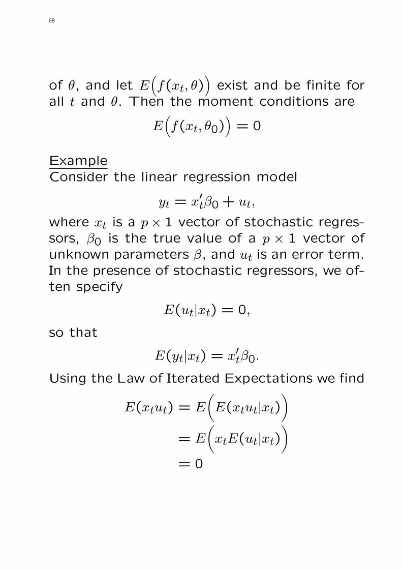
ExampleConsider the linear regression model
yt = x′tβ0 + ut,
where xt is a p× 1 vector of stochastic regres-sors, β0 is the true value of a p × 1 vector ofunknown parameters β, and ut is an error term.In the presence of stochastic regressors, we of-ten specify
E(ut|xt) = 0,
so that
E(yt|xt) = x′tβ0.
Using the Law of Iterated Expectations we find
E(xtut) = E
(E(xtut|xt)
)= E
(xtE(ut|xt)
)= 0
69

The equations
E(xtut) = E
(xt(yt − x′tβ0)
)= 0,
are moment conditions for this model. That is,θ = β and f
((xt, yt), θ
)= xt(yt − x′tβ).
Notice that in this example E(xtut) = 0 con-sists of p equations since xt is a p × 1 vector.Since β is a p × 1 parameter, these momentconditions exactly identify β. If we had fewerthan p moment conditions, then we could notidentify β, and if we had more than p momentconditions, then β would be over–identified.Estimation is feasible if the parameter vectoris exactly or over–identified.Compared to the maximum likelihood approach(ML), we have specified relatively little infor-mation about ut. Using ML, we would be re-quired to give the distribution of ut, as wellas parameterising any autocorrelation and het-eroskedasticity, while this information is not re-quired in formulating the moment conditions.
70

The MM estimation
Consider first the case when q = p, that is,
where θ is exactly identified by the moment
conditions. Then the moment conditions
E(f(xt, θ)
)= 0
represent a set of p equations for p unknowns.
Solving these equations would give the value of
θ which satisfies the moment conditions, and
this would be the true value θ0. However, we
cannot observe E(f(., .)
), only f(xt, θ). The ob-
vious way to proceed is to define the sample
moments of f(xt, θ)
fT (θ) = T−1T∑
t=1
f(xt, θ),
which is the Method of Moments (MM) esti-
mator of E(f(xt, θ)
).
Example 1
For the linear regression model, the sample
71

moment conditions are
T−1T∑
t=1
xtut = T−1T∑
t=1
xt(yt − x′tβT ) = 0,
and solving for βT gives
β =
T∑t=1
xtx′t
−1 T∑t=1
xtyt = (X ′X)−1X ′y.
That is, OLS is an MM estimator.
Example 2
The linear regression with q = p instrumental
variables is also exactly identified. The sample
moment conditions are
T−1T∑
t=1
ztut = T−1T∑
t=1
zt(yt − x′tβT ) = 0,
and solving for β gives
β =
T∑t=1
ztx′t
−1 T∑t=1
ztyt = (Z′X)−1Z′y,
72

which is the standard IV estimator.
Example 3
The Maximum Likelihood estimator can be given
an MM interpretation. If the log–likelihood for
a single observation is denoted l(θ|xt), then the
sample log–likelihood is T−1∑Tt=1 l(θ|xt). The
first order conditions for the maximisation of
the log–likelihood function are then
T−1T∑
t=1
∂l(θ|xt)∂θ
|θ=θT
= 0.
These first order conditions can be regarded
as a set of moment conditions.
The GMM
The GMM estimator is used when the θ param-
eters are over–identified by the moment condi-
tions, i.e., there are more moment conditions
73
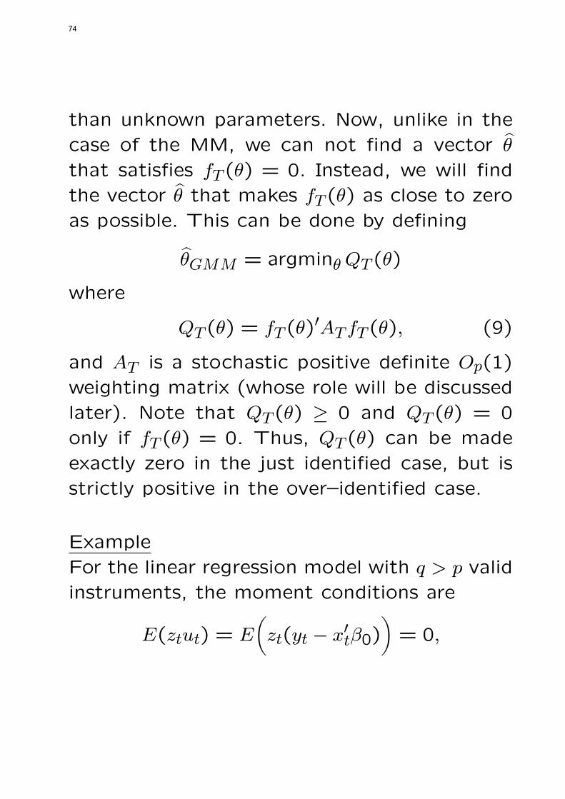
than unknown parameters. Now, unlike in the
case of the MM, we can not find a vector θ
that satisfies fT (θ) = 0. Instead, we will find
the vector θ that makes fT (θ) as close to zero
as possible. This can be done by defining
θGMM = argminθQT (θ)
where
QT (θ) = fT (θ)′ATfT (θ), (9)
and AT is a stochastic positive definite Op(1)
weighting matrix (whose role will be discussed
later). Note that QT (θ) ≥ 0 and QT (θ) = 0
only if fT (θ) = 0. Thus, QT (θ) can be made
exactly zero in the just identified case, but is
strictly positive in the over–identified case.
Example
For the linear regression model with q > p validinstruments, the moment conditions are
E(ztut) = E
(zt(yt − x′tβ0)
)= 0,
74

and the sample moments are
fT (β) = T−1T∑
t=1
zt(yt−x′tβ) = T−1(Z′y−Z′Xβ).
Suppose we choose
AT =
T−1T∑
t=1
ztz′t
−1
= T (Z′Z)−1,
and assume we have a weak law of large num-
bers for ztz′t so that T−1Z′Z converges in prob-
ability to a constant matrix A. Then the crite-
rion function is
QT (β) = T−1(Z′y−Z′Xβ)′(Z′Z)−1(Z′y−Z′Xβ).
Differentiating with respect to β gives
∂QT (β)
∂β= T−12X ′Z(Z′Z)−1(Z′y − Z′Xβ) = 0.
Setting this derivative to zero and solving for
βT gives
βT =(X ′Z(Z′Z)−1Z′X
)−1X ′Z(Z′Z)−1Z′y.
75
This is the standard IV estimator for the case
where there are more instruments than regres-
sors.
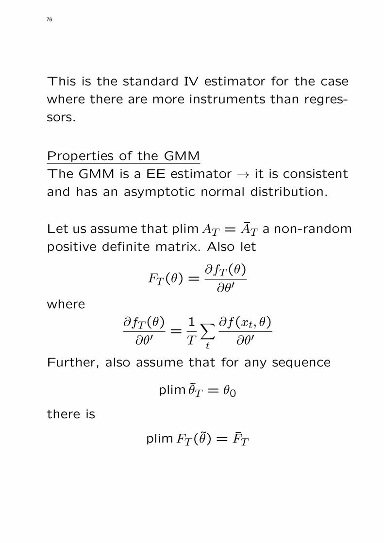
Properties of the GMM
The GMM is a EE estimator → it is consistent
and has an asymptotic normal distribution.
Let us assume that plimAT = AT a non-random
positive definite matrix. Also let
FT (θ) =∂fT (θ)
∂θ′
where
∂fT (θ)
∂θ′=
1
T
∑t
∂f(xt, θ)
∂θ′
Further, also assume that for any sequence
plim θT = θ0
there is
plimFT (θ) = FT
76
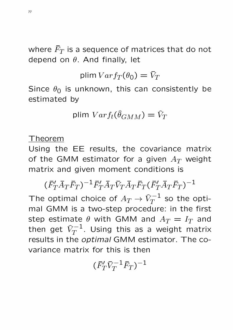
where FT is a sequence of matrices that do notdepend on θ. And finally, let
plimV arfT (θ0) = VT
Since θ0 is unknown, this can consistently beestimated by
plim V arft(θGMM) = VT
TheoremUsing the EE results, the covariance matrixof the GMM estimator for a given AT weightmatrix and given moment conditions is
(F ′T AT FT )
−1F ′T AT VT AT FT (F
′T AT FT )
−1
The optimal choice of AT → V −1T so the opti-
mal GMM is a two-step procedure: in the firststep estimate θ with GMM and AT = IT andthen get V −1
T . Using this as a weight matrixresults in the optimal GMM estimator. The co-variance matrix for this is then
(F ′T V
−1T FT )
−1
77

.
Testing for over-identifying restrictions
This is in fact specification testing.
The idea: Divide the restrictions (for “historic”
reasons we talk usually here of “restrictions”
while in fact we mean moment or orthogonality
conditions) into two groups: identifying restric-
tion and over-identifying restrictions. Estimate
the unknown parameters using the identifying
restriction and then test whether the estimated
parameters satisfy the over-identifying ones. If
so the identification is regarded as correct.
Assume that θT is the estimated parameter ob-
tained using GMM and the identifying restric-
tions. Then the test statistic
JT = QT (θT )A∼ χ2
q−p
78

where QT is (9), q is the number of over-identifying restrictions and p is the number ofparameters.
A special case of this test is the Hausman spec-ification test:
H0 : ML and E(f(xt, θ0)) = 0 are correct
HA : only E(f(xt, θ0)) = 0 is correct
Then the test statistic is
HT = (θT,ML − θT,GMM)′(VT,ML − VT,GMM)−1 .
. (θT,ML − θT,GMM)A∼ χ2
p
where V are consistent estimator of the respec-tive covariance matrices. In the original Haus-man paper the OLS and IV estimation werecompared → with the null that both the OLSand IV are consistent so there is no measure-ment error.
Let us have a look at another version of thetesting for over ident. restrictions called con-ditional moment test.
79

Let us have a model estimated by ML. Theconditional density of the explanatory variableXt, given the sample is pt(xt, θ0) and E[Lt(θ0)] =0 where now
Lt(θ0) =∂ ln(pt(xt, θ0))
∂θ
which (as seen in earlier lectures) are the or-thogonality conditions on which the ML is based.Now assume that if the model is correctly spec-ified, the data also satisfy the (q × 1) momentconditions E[f(xt, θ0)] = 0. So we would liketo test the null hypothesis
H0 : E[f(xt, θ0)] = 0
The test statistic now is
CMT =1
T
∑t
h(θT,ML)′V −1
T ×
× h(θT,ML)A∼ χ2
q
where
ht(θ) = [f(xt, θ)′, Ft(θ)
′]′
and VT is a consistent estimator of lim V ar(ht(θ0)).
80
Topic : 9
Biased Estimation
81

Biased estimation
A good estimator → likely to be in a small
neighbourhood of the true parameter value with
high probability. A biased estimator therefore
may be better than an unbiased one as the
smaller 2nd moment may “compensate” for
the inaccuracy caused by the bias.
Definition: Loss function: A function of the un-
known parameters of the model, their estima-
tor(s) and other parameters which expresses
the difference between the parameter estimates
and the true parameter values. → Reflects the
loss caused by the imprecision of an estimator.
Definition: Risk function: The expected value
of the Loss function (expected loss) → this in
fact measure the “goodness” of an estimator,
the smaller the risk the better.
82

Example: Weighted quadratic loss
L(β, β) = (β − β)′W (β − β)
if W = I we talk about squared error loss. Let
us have the “usual” linear model and we are
looking for an estimator of the form β = Ay
with the smallest risk.
minβ
E[(β − β)′(β − β)] = σ2tr(A′A)+
β′(AX − I)′(AX − I)β
which of course gives A = (X ′X)−1X.
The most straightforward way to improve on
any estimation is to use additional information.
The simplest way is to include in the estimation
process some parameter restrictions:
Rβ = r
where R is a known matrix of size (J×K), r is
a known vector of size (J ×1) both containing
83

the prior information, with J the number of
restrictions. So we want to estimate the model
y = Xβ+u under the restrictions Rβ = r which
will result in the called Restricted estimator:
minβ
(y−XβRLS)′(y−XβRLS) subject to Rβ = r
Using the Lagrangian formulation
L∗ = (y −XβRLS)′(y −XβRLS)− 2λ′(Rβ − r)
∂L∗
∂β= −2X ′(y −Xβ)− 2R′λ = 0
∂L∗
∂λ= 2(RβRLS − r) = 0
which gives
βRLS = βOLS + (X ′X)−1R′λ
Solving this for λ → pre-multiply by R and
Rβ = r is satisfied:
RβRLS = RβOLS +R(X ′X)−1R′λ = r
λ = −[R(X ′X)−1R′]−1[RβOLS − r]
84

That is
βRLS = βOLS + (X ′X)−1R[R(X ′X)−1R′]−1××(r −RβOLS)
Now about its properties. The 1st moment is
E(βRLS) = β + (X ′X)−1X ′u+
+ (X ′X)−1R[R(X ′X)−1R′]−1×× [r −R(X ′X)−1X ′Xβ +R(X ′X)−1X ′u]
= β +(I − (X ′X)−1R′[R(X ′X)−1R′]−1R
)×
× (X ′X)−1X ′u
This means that the estimator is unbiased onlyif RβRLS = r, i.e., the restrictions are true/correctin the sample. Then RβOLS = r and βRLS =βOLS.Let us turn now to the 2nd moment
E[(βRLS − β)(βRLS − β)′] =(I − (X ′X)−1R′[R(X ′X)−1R′]−1R
)(X ′X)−1X ′u︸ ︷︷ ︸
A
A′
= σ2(X ′X)−1××(I −R′[R(X ′X)−1R′]−1R(X ′X)−1
)
85
It can be shown that thew difference between
the covariance matrix of the OLS estimator
σ2(X ′X)−1 and the of the RLS is positive semi-
definite. This means that the variance of the
RLS is less than equal to the variance of the
OLS. When the restrictions are true/correct in
the sample the RLS is BLUE, consistent and
asymptotically efficient, using the information
in the sample and the restrictions.
The next question is what is going to hap-
pen when the restrictions are not true/correct,
Rβ − r = 0, Rβ − r = δ?! Obviously RLS → bi-
ased.
Intuition: If the restrictions are “somewhat”
not correct, although the RLS is biased, we
still may be better of using it, as the smaller
bias may “compensate” for this. So the valid-
ity of the restriction should be tested in the
sample.
86
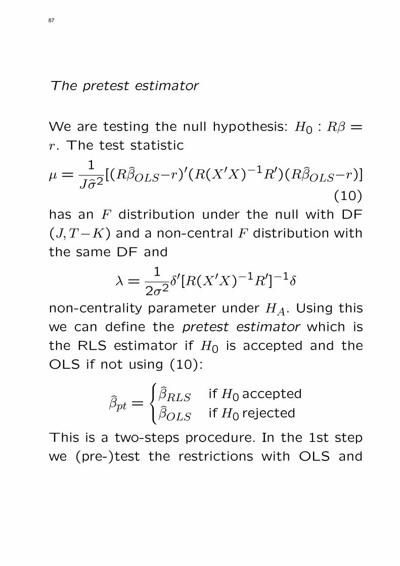
The pretest estimator
We are testing the null hypothesis: H0 : Rβ =
r. The test statistic
µ =1
Jσ2[(RβOLS−r)′(R(X ′X)−1R′)(RβOLS−r)]
(10)
has an F distribution under the null with DF
(J, T−K) and a non-central F distribution with
the same DF and
λ =1
2σ2δ′[R(X ′X)−1R′]−1δ
non-centrality parameter under HA. Using this
we can define the pretest estimator which is
the RLS estimator if H0 is accepted and the
OLS if not using (10):
βpt =
βRLS if H0 accepted
βOLS if H0 rejected
This is a two-steps procedure. In the 1st step
we (pre-)test the restrictions with OLS and
87

(10) and in the 2nd step, depending on the
outcome, the RLS or OLS is applied for infer-
ence.
1. If δ = 0 the pretest estimator is unbiased.
2. The risk of the pretest estimator, based on
the weighted quadratic loss, is smaller that the
risk of the OLS and is a decreasing function
of the critical value of the test (10).
3.With the increase of δ the risk of the pretest
estimator increases, but after reaching its max-
imum (which is higher that that of the OLS)
it decreases to the level of the OLS.
Stochastic restrictions
Assume now that our prior information, i.e.,
our restrictions are not deterministic, but stochas-
tic:
r = Rβ + v
where v is a vector of random variables, E(v) =
0 and E(vv′) = Ψ. Taking our usual linear
88
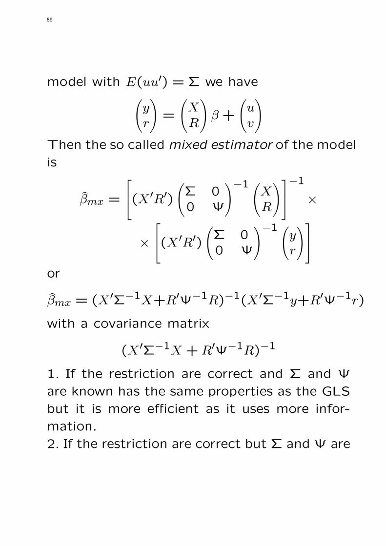
model with E(uu′) = Σ we have(yr
)=
(XR
)β +
(uv
)Then the so called mixed estimator of the model
is
βmx =
(X ′R′)
(Σ 00 Ψ
)−1(XR
)−1
×
×
(X ′R′)
(Σ 00 Ψ
)−1(yr
)or
βmx = (X ′Σ−1X+R′Ψ−1R)−1(X ′Σ−1y+R′Ψ−1r)
with a covariance matrix
(X ′Σ−1X +R′Ψ−1R)−1
1. If the restriction are correct and Σ and Ψ
are known has the same properties as the GLS
but it is more efficient as it uses more infor-
mation.
2. If the restriction are correct but Σ and Ψ are
89

unknown, if we have consistent estimators of
them, by using them the mx estimator is going
to have the same properties as the FGLS but
it is going to be asymptotically more efficient.
3. If the variance of v → 0, i.e., the prior infor-
mation becomes deterministic, the mixed esti-
mator approaches the restricted one.
4. If the variance of v → ∞, i.e., the prior in-
formation becomes diffuse or non-informative
the mixed estimator approaches the OLS.
The pretest estimator related to stochastic re-
strictions is testing H0 : E(r − Rβ) = δ = 0
with
µ =1
σ2[(r −RβOLS)
′(R(X ′X)−1R′ +Ψ)−1×
× (r −RβOLS)]
which has a χ2(J) under the null. If the vari-
ances are estimated we end up with an F dis-
tribution.
90

Topic : 10
Some Non-linear Models
91

Non-Nested model selection
Non-nested model selection most frequently is
base on information criteria.
To start with, let us remind ourselves the KL
measure, see when we dealt with the Pseudo
ML: The Kullback–Leibler index/measure of
proximity or discrepancy measures the simi-
larity between two distributions/densities. Let
g(y) and f(y, θ) be two probability distributions
for the random variable Y . The KL index is:
KL(g(.), f(.)) =∫yg(y) ln
g(y)
f(y, θ)d y =
= Eg[ln(g(y)/f(y, θ))] =
=∫yg(y) ln(g(y))d y︸ ︷︷ ︸
A
−∫yg(y) ln f(y, θ)d y︸ ︷︷ ︸
B
where Eg[.] denotes the expectation taken with
respect to the density g(y), which is the true
unknown distribution of y. f(y, θ) is the para-
metric distribution of the model, θ is the ML
92

estimate of the unknown parameters. The smaller
KL the closer the model is to the true distri-
bution. Task → find an f(y, θ) that min KL
→ minf B, as A is a constant from the view
point of this operation. Unfortunately this is
not possible as g(y) is unknown.
Different information criteria are drawn by “es-
timating” this B.
1.
B = −2 ln
L(y,θ)︷ ︸︸ ︷f(y, θ)+2j
where j is the size of θ. This is the so called
Akaike Information Criteria – AIC.
Model selection → calculate the AIC for all rel-
evant model alternatives and pick the model
with the smallest AIC
2. In many application the above B is consid-
ered “biased”. So there are alternatives, mostly
by using different “penalties” on the likelihood:
B = −Ln(y, θ) +j
2lnn
93

which is the Bayesian (Schwartz) Information
criteria or BIC.
Binary choice models – a quick reminder
y =
1 Prob(y = 1) = f(β′x)
0 Prob(y = 0) = 1− f(β′x)
Linear probability model: f(β′x) = β′x:1. No linear model would generate such depen-
dent variable.
2. Can yield negative probabilities, β′x may not
be in (01).
3. There is heteroscedasticity → V ar(u) = β′x(1−β′x).So why so people still use it? Because in a
non-linear model
∂E(y)
∂x= f ′(β′x)β
not the marginal effect we are used to → it
varies with x, which can be inconvenient in
some applications.
94
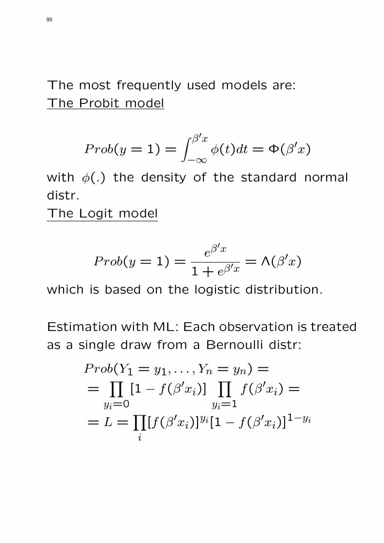
The most frequently used models are:
The Probit model
Prob(y = 1) =∫ β′x
−∞ϕ(t)dt = Φ(β′x)
with ϕ(.) the density of the standard normal
distr.
The Logit model
Prob(y = 1) =eβ
′x
1+ eβ′x
= Λ(β′x)
which is based on the logistic distribution.
Estimation with ML: Each observation is treated
as a single draw from a Bernoulli distr:
Prob(Y1 = y1, . . . , Yn = yn) =
=∏
yi=0
[1− f(β′xi)]∏
yi=1
f(β′xi) =
= L =∏i
[f(β′xi)]yi[1− f(β′xi)]
1−yi
95
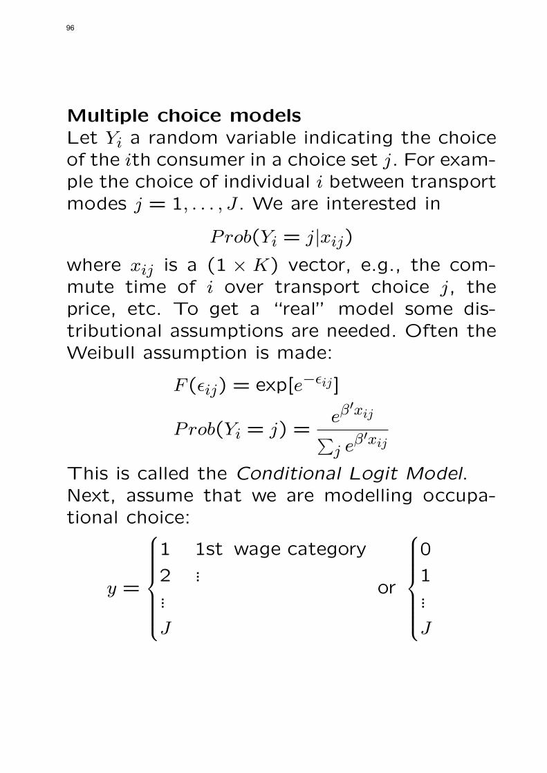
Multiple choice modelsLet Yi a random variable indicating the choiceof the ith consumer in a choice set j. For exam-ple the choice of individual i between transportmodes j = 1, . . . , J. We are interested in
Prob(Yi = j|xij)where xij is a (1 × K) vector, e.g., the com-mute time of i over transport choice j, theprice, etc. To get a “real” model some dis-tributional assumptions are needed. Often theWeibull assumption is made:
F (ϵij) = exp[e−ϵij]
Prob(Yi = j) =eβ
′xij∑j e
β′xij
This is called the Conditional Logit Model.Next, assume that we are modelling occupa-tional choice:
y =
1 1st wage category
2 ......
J
or
0
1...
J
96

This type of problem is dealt with the Multi-
nomial logit model: Assuming again a Weibull
distribution
Prob(Yi = j) =eβ′jxi
J∑k=0
eβ′kxi
To make the model identified some some re-
strictions on the βs are needed, like β0 = 0.
Then
Prob(Yi = j) =eβ′jxi
1+J∑
k=1eβ
′kxi
j = 1, . . . , J
and
Prob(Yi = 0) =1
1+J∑
k=1eβ
′kxi
97

The log-likelihood now is
ln∑i
J∑j=0
dijProb(Yi = j)
dij
1 if i choses j
0 otherwise
When normalized at β0 = 0 the jth log-odd
ratio is
ln
[Pij
Pi0
]= β′
jxi
when we normalize on any other parameter
(say the k-th)
ln
[Pij
Pik
]= x′i(β
′j − βk)
The odds ratios do not depend on the other
choices (what the others have chosen). This is
called the Independence of Irrelevant Alterna-
tives.
98

Ordered multiple choice models
The model again is y∗ = β′x+ ϵ, but y∗ is not
observed, instead we observe, for example,
y = 0 if y∗ ≤ 0
y = 1 if 0 < y∗ ≤ µ1...
y = J if µJ−1 ≤ y∗
where the µ-s can be known or unknown! Es-
timation → standard ML!
Let us make now a technical detour! Condi-
tional distribution.
When r.v X and Y are a bivariate normal dis-
tribution, the have the following joint density
f(x, y) =1
2πσxσy
exp[−
1
2(1− ρ2)[(x− µx
σx)2 + (
y − µy
σy)2
− 2ρ(x− µx
σx)(
y − µy
σy)]]
99

where ρ is the correlation between X and Y .
This joint density can be re-written as
f(x, y) = f(y|x)︸ ︷︷ ︸conditional
.
marginal︷ ︸︸ ︷f1(x) =
=1
√2πσy
√1− ρ2
exp[−
1
2σ2y(1− ρ2)
[y − µy − ρσy
σx(x− µx)]
2]×
×1√2πσx
exp[−1
2σ2y(x− µx)
2]
Let us next turn to the conditional moments.
The conditional 1st moment is
E(y|x) =∫yyf(y|x)dy
when y is continuous and
E(y|x) =∑y
yf(y|x)
when y is discrete. the conditional variance now
100
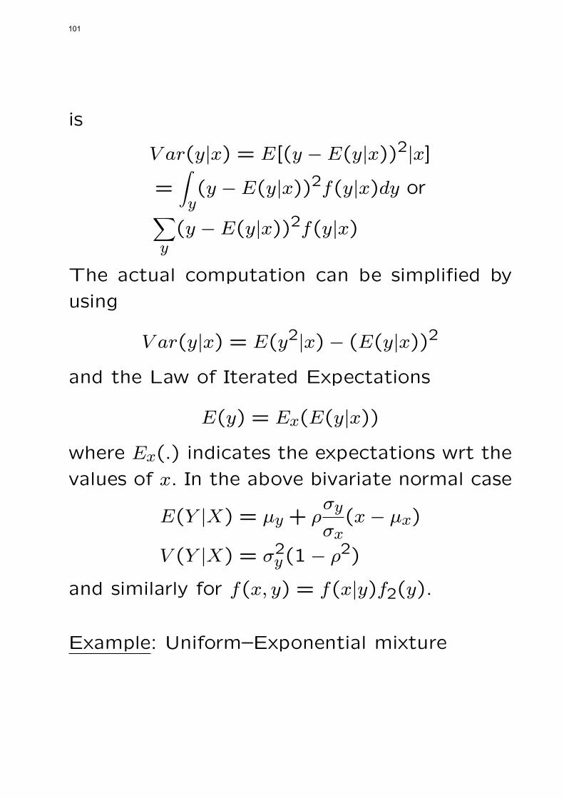
is
V ar(y|x) = E[(y − E(y|x))2|x]
=∫y(y − E(y|x))2f(y|x)dy or∑
y(y − E(y|x))2f(y|x)
The actual computation can be simplified by
using
V ar(y|x) = E(y2|x)− (E(y|x))2
and the Law of Iterated Expectations
E(y) = Ex(E(y|x))
where Ex(.) indicates the expectations wrt the
values of x. In the above bivariate normal case
E(Y |X) = µy + ρσy
σx(x− µx)
V (Y |X) = σ2y(1− ρ2)
and similarly for f(x, y) = f(x|y)f2(y).
Example: Uniform–Exponential mixture
101

f(y|x) =1
α+ βxexp[−
y
α+ βx]
y ≤ 0, 0 ≤ x ≤ 1
E(y|x) = α+ βx
if x is uniform (0,1) the f(x) = 1. f(x, y) =f(y|x)f(x) so
E(y) =∫ ∞
0
∫ 1
0y(
1
α+ βx).
. exp[−y
α+ βx]dx dy
So
E(y) = Ex(E(y|x))= E(α+ βx)
= α+ β E(x)︸ ︷︷ ︸1/2
= α+ β1/2
Now about the variance
V ar(y) = V arx(E(y|x)) + Ex(V ar(y|x))
102

So
V ar(y) = α(α+ β) +5β2
12
Truncation
For example: incomes over/below a given limit
are not observed, etc.
Definition: Truncated distribution: part of an
un-truncated distribution, above or below some
specific values.
Definition: Density of a truncated r.v.:
If continuous r.v. x has a pdf f(x) and a is a
constant
f(x|x > a) =f(x)
Prob(x > a)
which amounts to nothing more that scaling
the density so its∫= 1. (Truncated from above
→ the same.)
103

Example: Uniform x truncated at 1/3.
So x is U(01), f(x) = 1
f(x|x >1
3) =
f(x)
Prob(x > 13)
=123
,1
3< x ≤ 1
1st moment of a truncated r.v.
E(x|x > a) =∫ ∞
axf(x|x > a)dx
Example: Uniform distribution
E(x|x >1
3) =
∫ 1
1/3x(.)dx =
2
3
For the variance calculations are similar.
Truncation from below → increases mean
Truncation from above → decreases mean
Truncation → reduces variance.
104

Truncated normal distr:
Prob(x > a) = 1−Φ(a− µ
σ)
= 1−Φ(α)
f(x|x > a) =f(x)
1−Φ(α)
where Φ(.) is the normal cdf.
E(x|x > a) = µ+ σλ(α)
V ar(x|x > a) = σ2(1− δ(α))
with
λ(α) =ϕ(α)
1−Φ(α)if x > a
λ(α) = −ϕ(α)
Φ(α)if x < a
δ(α) = λ(α)(λ(α)− α) and
0 < δ(α) < 1 ∀αand λ(α) → inverse Mills ratio.
Truncated regression.
yi = β′xi + εi
105

εi ∼ N(0, σ2) →(yi|xi) ∼ N(β′xi, σ2). With a truncation point a
E(yi|yi > a) = β′xi + σ
λi︷ ︸︸ ︷λ(αi)
αi =a− β′xi
σV ar(yi|yi > a) = σ2(1− δ(αi))
LS estimation
(yi|yi > a) = β′xi + σλi + ui
where σλi is a function of x and if omitted →omitted variable bias; and ui is heteroscedastic:
V ar(ui) = σ2(1− λ2i + λiαi)
ML estimation
f(yi|yi > a) =1σϕ(yi − β′xi)/σ)
1−Φ(a− β′xi)/σ)
106

lnL = −n
2[ln(2π) + lnσ2]−
−1
2σ2∑i
(yi − β′xi)2−
−∑i
ln[1−Φ(a− β′xi
σ)] → max
Censoring
Let us have a continuous r.v y∗ and a new one
y transformed from the original as
y = 0 if y∗ ≤ 0
y = y∗ if y∗ > 0(11)
This is censoring at 0, but it can be at any
other value.
Lemma:
If y∗ ∼ N(µ, σ2) then
Prob(y = 0) = Prob(y∗ ≤ 0)
= 1−Φ(µ
σ)
and if y∗ > 0 y has the density of y∗. → mix-
ture of continuous and discrete distributions.
107
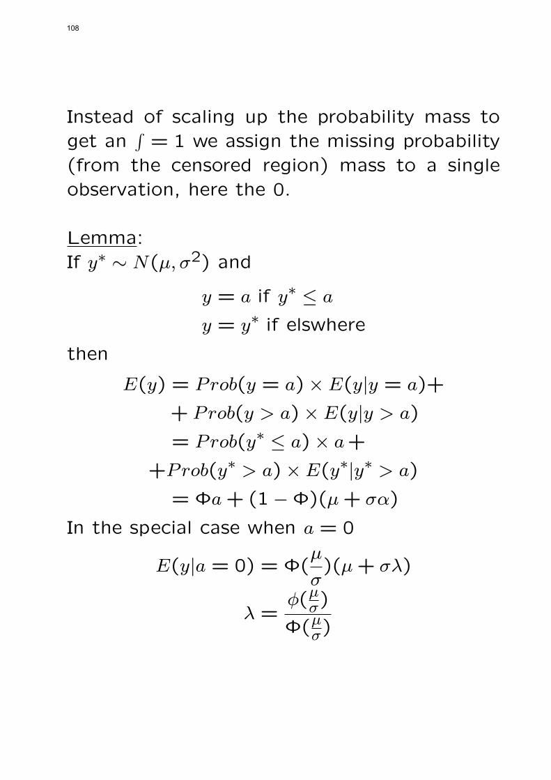
Instead of scaling up the probability mass toget an
∫= 1 we assign the missing probability
(from the censored region) mass to a singleobservation, here the 0.
Lemma:If y∗ ∼ N(µ, σ2) and
y = a if y∗ ≤ a
y = y∗ if elswhere
then
E(y) = Prob(y = a)× E(y|y = a)+
+ Prob(y > a)× E(y|y > a)
= Prob(y∗ ≤ a)× a+
+Prob(y∗ > a)× E(y∗|y∗ > a)
= Φa+ (1−Φ)(µ+ σα)
In the special case when a = 0
E(y|a = 0) = Φ(µ
σ)(µ+ σλ)
λ =ϕ(µσ)
Φ(µσ)
108

And for the variance
V ar(y) = σ2(1−Φ)((1− δ) + (α− λ)2Φ)
where
Φ = Φ(α) = Prob(y∗ ≤ a)
= Φ(a− µ
σ)
λ =ϕ
1−Φand
δ = λ2 − λα
Censored regression (the Tobit model)
Let us have now a linear regression model with
dependent variable as in (11):
E(yi|xi) = Φ(β′xiσ
)(β′xi + σλi)
λi =ϕ(β
′xiσ )
1−Φ(β′xiσ )
109
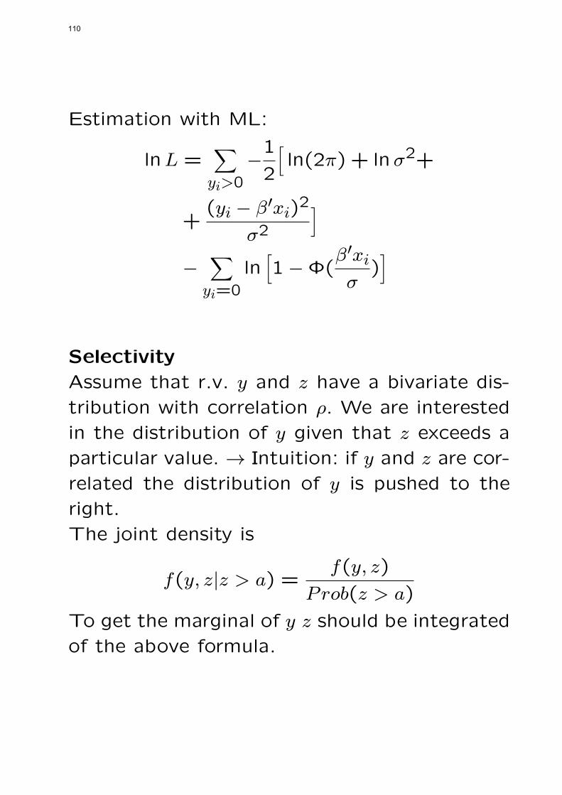
Estimation with ML:
lnL =∑yi>0
−1
2
[ln(2π) + lnσ2+
+(yi − β′xi)2
σ2
]−
∑yi=0
ln[1−Φ(
β′xiσ
)]
Selectivity
Assume that r.v. y and z have a bivariate dis-
tribution with correlation ρ. We are interested
in the distribution of y given that z exceeds a
particular value. → Intuition: if y and z are cor-
related the distribution of y is pushed to the
right.
The joint density is
f(y, z|z > a) =f(y, z)
Prob(z > a)
To get the marginal of y z should be integrated
of the above formula.
110

Theorem: Moments of a bivariate normal dis-
tribution with selectivity (also called: incidental
truncation):
E(y|z > a) = µy + ρσyλ(αz)
V ar(y|z > a) = σ2y(1− ρ2δ(αz)) where
αz =a− µz
σz
λ(αz) =ϕ(αz)
1−Φ(αz)and
δ(αz) = λ(αz)(λ(αz)− αz)
which is similar to the truncation → if ρ = 0
we get back the “usual” case, when ρ = 1 we
get back the truncation case.
Regression with selectivity (or incidental trun-
cation):
yi = β′xi + ϵi focus equation
z∗i = γ′wi + ui selection equation(12)
and yi is only observed when z∗i > 0. Now as-
sume that ui and ϵi are bivariate normal with
111

correlation ρ. Then
E(yi|yi is observed) = E(yi|z∗i > 0)
= E(yi|ui > −γ′wi)
= β′xi + E(ϵi|ui > −γ′wi)
= β′xi + ρσϵ︸︷︷︸βλ
λi(αu) where
αu = −γ′wi
σuand
λ(αu) =ϕ(γ′wi/σu)
Φ(γ′wi/σu)
So the model with selectivity is
(yi|z∗i > 0) = β′xi + β′λλi(αu) + vi (13)
Estimation: ML or the Heckman two-step pro-cedure:1. Estimate the selection equation by ML andthe compute
λi =ϕ(γ′MLwi)
Φ(γ′MLwi)
and
δ∗i = λi(λi + γ′wi)
112

2. Estimate (13) using λi and δi.
The Heckman 2-step procedure is consistent,
but the standard errors need to be corrected
as there is heteroscedasticity.
Nonresponse – Ignorable selectivity
The most important types of nonresponse that
can occur in panel data sets (and mostly in
other types of data sets as well)
1. Initial nonresponse occurs when individu-
als contacted for the first time refuse (or
are not able) to cooperate with the sur-
vey, or—for some reason—can not be con-
tacted at all. Because only very limited in-
formation is recorded for this group of non-
respondents this type of nonresponse is one
of the most difficult to deal with during
the analysis stage. Usually, the researcher
is not even aware of the problem of initial
113
nonresponse and implicitly assumes that it
does not distort his analysis.
2. Unit nonresponse is initial nonresponse that
results in missing data on all variables for
a particular unit. Only in cases where the
persons in question are interviewed at a
later stage both concepts do not coincide.
3. Item nonresponse occurs when information
on a particular variable for some individ-
ual is missing. For example, individuals may
refuse to report their income, while provid-
ing data for all other questions, like age,
education, family size, expenditure patterns,
etc.
4. Wave nonresponse is typical for panel data
and occurs when units do not respond for
114
one or more waves but participate in the
preceding and succeeding wave. In a monthly
panel a typical situation where this occurs
is that where an individual is on vacation
for a couple of weeks.
5. Attrition occurs when individuals having par-
ticipated one or more waves leave the panel.
These individuals do not return in the panel.
This can be caused by removal, emigration
or decease, but also by the fact that indi-
viduals are just “tired” of answering similar
questions each time.
Standard econometric methods are usually based
on a rectangular data set in which no data are
missing. If a data set with missing values is
used, for example, in statistical software, usu-
ally all observations are discarded for which one
115

or more of the variables under analysis is miss-ing. This is not only inefficient (because in-formation loss), but, more importantly, the re-maining cases may no longer be representativefor the population. Therefore, it is importantfor a researcher to pay attention to the natureof the nonresponse whether selection is likelyto be present or not.
Now let us assume that in (12) the dependentvariable of the selection equation is a binaryvariable r = 1 if all our variables are observedand r = 0 if an observation for any of the vari-ables in the model is missing. Let us call theselection mechanism to be ignorable if con-ditioning on the response indicator variable r
does not affect the joint distribution of y andx, i.e., if
f(y, x | β) = f(y, x | r;β),which implies that r is independent of (y, z).This in practice can be tested with the use ofa binary choice model.
116
Topic : PD0
Matrix Algebra Notes for LinearPanel Data Models
117

In these notes we review the main matrices
used when dealing with linear models, their
behaviour and properties.∗
Notation
• A single parameter (or scalar) is always
a lower case Roman or Greek letter;
• A vector is always an underlined lower
case Roman or Greek letter;
• An element of a vector is [ai];
• A matrix is always an upper case letter;
• An element of a matrix is [aij];
∗This appendix is based on Alain Trognon’s unpub-lished manuscript.
118

• An estimated parameter, parameter vec-
tor or parameter matrix is denoted by a
hat;
• The identity matrix is denoted by I and
if necessary I with the appropriate size
(N ×N) → IN ;
• The unit vector (all elements = 1) of
size (N × 1) is denoted by lN and the
unit matrix of size (N × N) is denoted
by JN .
119

In a two-dimensional panel data set (2D) all
variables look like this:
x =
x11x12...
x1T...
xN1xN2...
xNT
or
[xit] i = 1, . . . , N t = 1, . . . , T
120

The matrices used
It is well known that the total variability of
a vector (of N individuals for T periods) can
be decomposed as∑i
∑t
(xit − x)2 =
∑i∑
t(xit − xi)2 + T
∑i(xi − x)2∑
i∑
t(xit − xt)2 +N∑
t(xt − x)2∑i∑
t(xit − xi − xt + x)2 + T∑
i(xi − x)2+
+N∑
t(xt − x)2 ,
where
xi =1T
∑t xit is the mean of the individual i,
xt =1N
∑i xit is the mean of the period t,
x = 1NT
∑i∑
t xit is the overall mean, and∑i∑
t(xit−x)2 is the total variability (around
the general mean),∑i∑
t(xit − xi)2 is the within individual vari-
ability,
T∑
i(xi − x)2 is the between individual vari-
ability,∑i∑
t(xit−xt)2 is the within period variabil-
ity,
121
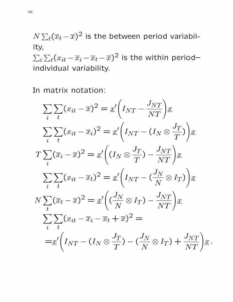
N∑
t(xt−x)2 is the between period variabil-
ity,∑i∑
t(xit−xi−xt−x)2 is the within period–
individual variability.
In matrix notation:∑i
∑t
(xit − x)2 = x′(INT −
JNT
NT
)x
∑i
∑t
(xit − xi)2 = x′
(INT − (IN ⊗
JTT
)
)x
T∑i
(xi − x)2 = x′((IN ⊗
JTT
)−JNT
NT
)x
∑i
∑t
(xit − xt)2 = x′
(INT − (
JNN
⊗ IT )
)x
N∑t
(xt − x)2 = x′((JNN
⊗ IT )−JNT
NT
)x∑
i
∑t
(xit − xi − xt + x)2 =
=x′(INT − (IN ⊗
JTT
)− (JNN
⊗ IT ) +JNT
NT
)x .
122

The abbreviation and the rank of these ma-
trices are
T ∗ = INT −JNT
NTrank :NT − 1
Bn = (IN ⊗JTT
)−JNT
NT= (IN −
JNN
)⊗JTT
rank :N − 1
Bt = (JNN
⊗ IT )−JNT
NT=
JNN
⊗ (IT −JTT
)
rank :T − 1
Wn = INT − (IN ⊗JTT
) = IN ⊗ (IT −JTT
)
rank :N(T − 1)
Wt = INT − (JNN
⊗ IT ) = (IN −JNN
)⊗ IT
rank :T (N − 1)
W ∗ = INT − (IN ⊗JTT
)− (JNN
⊗ IT ) +JNT
NT
= (IN −JNN
)⊗ (IT −JTT
)
rank : (N − 1)(T − 1).
123

These matrices can be considered as or-
thogonal projectors into a subspace of RNT ,
where the dimension of these subspaces equals
the rank of the projector.
The main properties of these projector ma-
trices are:
T ∗ =
Wn +Bn
Wt +Bt
W ∗ +Bn +Bt ,
and
WnBn = WtBt = W ∗Bn = W ∗Bt = BnBt = 0
T ∗JNT
NT= W ∗JNT
NT= Wn
JNT
NT=
= WtJNT
NT= Bn
JNT
NT= Bt
JNT
NT= 0 .
The matrices T ∗, W ∗, Wn, Wt, Bn, and Bt
are symmetric and idempotent.
124

For the non–centered case the variability de-composition is
∑i
∑t
x2it =
∑
i∑
t(xit − xi)2 + T
∑x2i∑
i∑
t(xit − xt)2 +N∑
x2t .
The necessary non–centered transformationmatrices are
T∗ = INT , Bn = IN ⊗
JTT
,
Bt =JNN
⊗ IT , W∗ = W ∗ +
JNT
NTWn = Wn, W t = Wt .
The total variability in this case is made upas
T∗ =
Wn +Bn
Wt +Bt
W∗ +Bn +Bt .
The properties of these matrices are:
WnBn = WtBt = 0
W∗Bn = W
∗Bt = 0
and T∗, Bn, and Bt are symmetric and idem-
potent.
125

Partitioned inverse of matrices
Let
B = A−1 =
[B11 B12B21 B22
], and
[A11 A12A21 A22
]Then
B11 =(A11 −A12A
−122A21
)−1
B12 = −A−111A12
(A22 −A21A
−111A12
)−1
B21 = −A−122A21
(A11 −A12A
−122A21
)−1
B22 =(A22 −A21A
−111A12
)−1
126

The necessary spectral decompositions
In the case of the error components mod-
els, in order to derive the GLS and FGLS
estimators it is necessary to elaborate the
inverse of the covariance matrix of the dis-
turbance terms. This is based on the spec-
tral decomposition of these matrices.
Assume we have a symmetric matrix S. De-
composition QSQ = Λ always exists, where
Q contains the orthogonal eigen vectors of
S and λ is diagonal with the eigen values in
its elements.
S = QΛQ =∑
λiqiq′i
where λi are the eigen values, and qi the
appropriate eigen vectors
127

Topic : PD1
Linear Panel Data Models withFixed Effects – FE Models
128

Model with individual effects only
Let the basic FE model be:
yit = αi + x′itβ + uit
the˜notes that x does not contain the col-
umn of 1-s of the regression constant. We
will not use this just “simply”
yit = αi + x′itβ + uit
where αi are the individual effects. In fact
the regression constant is broken up into N
fixed effects. For individual i the model is:
yi = lTαi +Xiβ + ui ,
where yi is the T × 1 vector of the yit, lT is
the unit vector of size T , Xi is the T×(K−1)
matrix whose t–th row is x′it and ui, is the
T × 1 vector of disturbances.
129
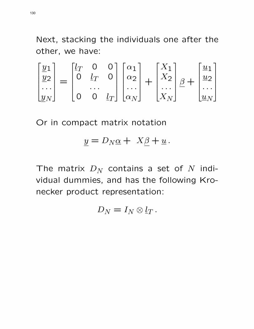
Next, stacking the individuals one after the
other, we have:y1y2. . .yN
=
lT 0 00 lT 0
. . .0 0 lT
α1α2. . .αN
+
X1X2. . .XN
β +
u1u2. . .uN
Or in compact matrix notation
y = DNα+ Xβ + u .
The matrix DN contains a set of N indi-
vidual dummies, and has the following Kro-
necker product representation:
DN = IN ⊗ lT .
130

It can easily be verified that the following
properties hold:
1. DN lN = lN ⊗ lT = lNT
2. D′NDN = TIN
3. DND′N = IN ⊗ lT l
′T = IN ⊗ JT
4. 1TD
′Ny = [y1, . . . , yN ]′
where yi =1T
∑Tt=1 yit and, by definition, JT =
lT l′T (the unit matrix of order T ).
131

Note (!!!):
We assume NT > N +K (which is satisfied
for large N whenever T ≥ 2), this requires
that the columns of X be linearly indepen-
dent from those of DN . For this to be the
case, the matrices Xi must not contain the
constant term (an obvious restriction) nor a
column proportional to it (which precludes
any variable, such as years of schooling, that
is constant for a given adult individual, al-
though varying from individual to individ-
ual).
Next let us turn to the estimation of this
model
132

y = DNα+ Xβ + u .
Let us simplify and not underline when not
really needed
y = (DN , X)
(αβ
)+ u (1)
y = (DN , X)γ + u
Estimating this model with OLS
γ =
[(D′
NX ′
)(DN , X)
]−1(D′
NX ′
)y =
[D′
NDN D′NX
X ′DN X ′X
]−1(D′
NX ′
)y
which gives
β = (X ′WnX)−1X ′Wny
This is called the WITHIN estimator!
133
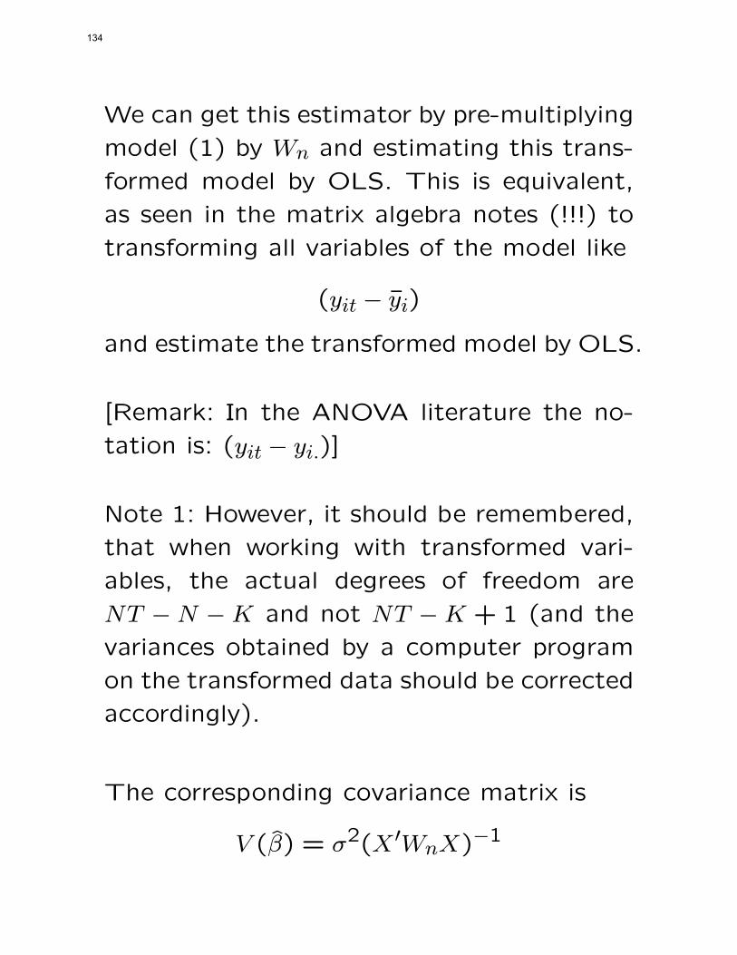
We can get this estimator by pre-multiplying
model (1) by Wn and estimating this trans-
formed model by OLS. This is equivalent,
as seen in the matrix algebra notes (!!!) to
transforming all variables of the model like
(yit − yi)
and estimate the transformed model by OLS.
[Remark: In the ANOVA literature the no-
tation is: (yit − yi.)]
Note 1: However, it should be remembered,
that when working with transformed vari-
ables, the actual degrees of freedom are
NT − N − K and not NT − K + 1 (and the
variances obtained by a computer program
on the transformed data should be corrected
accordingly).
The corresponding covariance matrix is
V (β) = σ2(X ′WnX)−1
134
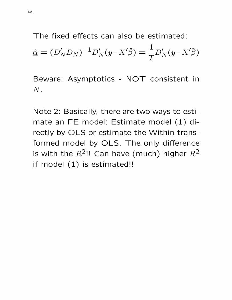
The fixed effects can also be estimated:
α = (D′NDN)−1D′
N(y−X ′β) =1
TD′
N(y−X ′β)
Beware: Asymptotics - NOT consistent in
N .
Note 2: Basically, there are two ways to esti-
mate an FE model: Estimate model (1) di-
rectly by OLS or estimate the Within trans-
formed model by OLS. The only difference
is with the R2!! Can have (much) higher R2
if model (1) is estimated!!
135
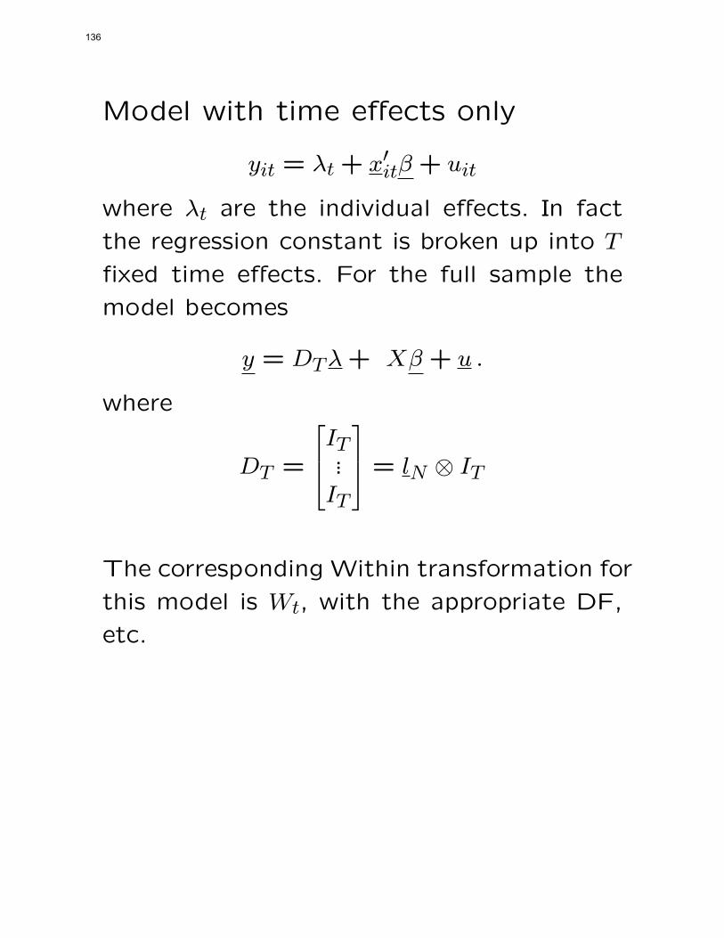
Model with time effects only
yit = λt + x′itβ + uit
where λt are the individual effects. In fact
the regression constant is broken up into T
fixed time effects. For the full sample the
model becomes
y = DTλ+ Xβ + u .
where
DT =
IT...IT
= lN ⊗ IT
The corresponding Within transformation for
this model is Wt, with the appropriate DF,
etc.
136

Model with individual and time ef-fects
yit = αi + λt + x′itβ + uit
or
y = DNα+DTλ+ Xβ + u .
Beware of the Dummy Variable Trap!!
Appropriate operator is the transformed W ∗,for identification.
Asymptotic properties: N → ∞ and T finite.
T → ∞ N finite. N and T go to ∞ then the
rates should be evaluated.
Separability of the parameter estimates!!
137

Some extensionsConstant Variables in One Dimension
The generic fixed individual effect consid-
ered may be the result of some factors (such
as sex, years of schooling, race, etc.) which
are constant through time for any individual
but vary across individuals. If observations
are available on such variables, we might
wish to incorporate them explicitly in the
regression equation. The model may thus
be written as:
yit = z′iδ + x′itβ + uit
where the row–vector z′i now contains the
observations on the variables which are con-
stant for individual i, including the constant
term, and δ is the associated vector of coef-
ficients. We assume that there are Kz such
variables.
138

Collecting the T observations for individual
i, we get:
yi = (z′i ⊗ lT )δ +Xiβ + ui
and, finally, stacking the N individuals, we
obtain the full model
y = (Z ⊗ lT )δ +Xiβ + u
where Z is the N × Kz matrix whose i–th
row is z′i.
Let us note that the columns of (Z⊗ lT ) are
linear combinations of the columns of the
matrix of individual dummies. In fact:
(Z ⊗ lT ) = (IN ⊗ lT )(Z ⊗ 1) = DNZ
139
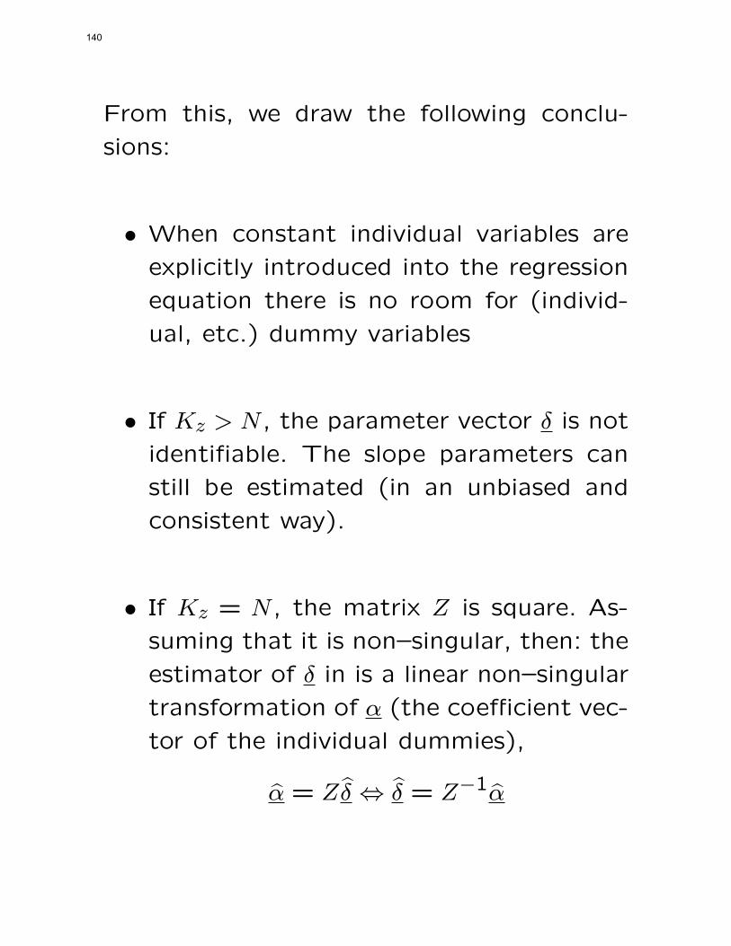
From this, we draw the following conclu-
sions:
• When constant individual variables are
explicitly introduced into the regression
equation there is no room for (individ-
ual, etc.) dummy variables
• If Kz > N , the parameter vector δ is not
identifiable. The slope parameters can
still be estimated (in an unbiased and
consistent way).
• If Kz = N , the matrix Z is square. As-
suming that it is non–singular, then: the
estimator of δ in is a linear non–singular
transformation of α (the coefficient vec-
tor of the individual dummies),
α = Zδ ⇔ δ = Z−1α
140

• If Kz < N , α = Zδ. When Kz < N , a
total of N −Kz restrictions are imposed
on the vector α, (F ′α = 0, where F ′ is a
(N−Kz)×N matrix of full rank such that
F ′Z = 0). Ignoring these restrictions on
α is like estimating a model with some
additional extraneous variables, which pro-
duces unbiased but inefficient estimates.
The same argument applies when the model
is extended to include variables that vary in
time, but that are constant for all individuals
(such as prices).
141

Topic : PD2
Linear Panel Data Models withRandom Effects – RE Models (alsocalled Error Components Models –
EC Models)
142
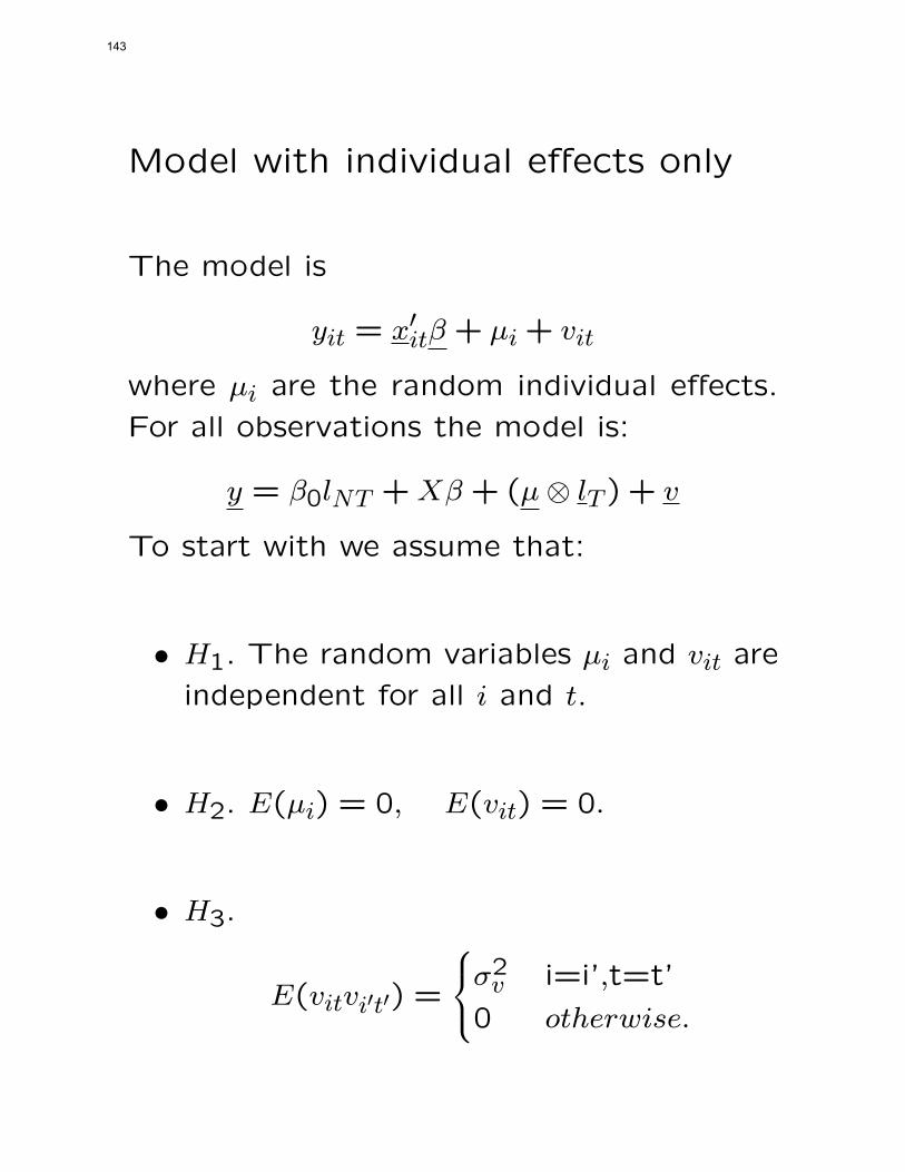
Model with individual effects only
The model is
yit = x′itβ + µi + vit
where µi are the random individual effects.
For all observations the model is:
y = β0lNT +Xβ + (µ⊗ lT ) + v
To start with we assume that:
• H1. The random variables µi and vit are
independent for all i and t.
• H2. E(µi) = 0, E(vit) = 0.
• H3.
E(vitvi′t′) =
σ2v i=i’,t=t’
0 otherwise.
143

• H4.
E(µiµi′) =
σ2µ i=i
0 otherwise.
• H5.
vit ∼ N (0, σ2v ) .
• H6. The random variable µi (∀i) has a
normal distribution, µi ∼ N (0, σ2µ).
• H7. The matrix of the regressors X is
non-stochastic.
144

If we introduce time effects as well into the
model we have
yit = x′itβ + µi + εt + vit
and so get
u = µ⊗ lT + (lN ⊗ IT )ε+ v ,
where ε is the random vector of time effects
(T×1). As in the previous model we assume
that µ, ε and v are mutually independent,
with 0 expected values, σ2ε is normally dis-
tributed, and
E(µµ′) = σ2µIN , E(εε′) = σ2ε IT , E(vv′) = σ2v INT .
Since the individual and time effects are in-
corporated in the model through the resid-
ual (error) structure, our main interest has
to be focused on the covariance matrix of
the residual (error) term.
145

If only individual effects are present, then
for the individual i the covariance matrix is
E(uiu′i) = σ2µJT + σ2v IT = Σ ,
and, taking into account the properties of
the projection matrices Wn and Bn for all
individuals,
E(uu′) = σ2vWn + (σ2v + Tσ2µ)Bn = Ω .
In the case when time effects are also present
E(uu′) = σ2µ(IN⊗JT )+σ2ε (JN⊗IT )+σ2v INT = Ω .
146
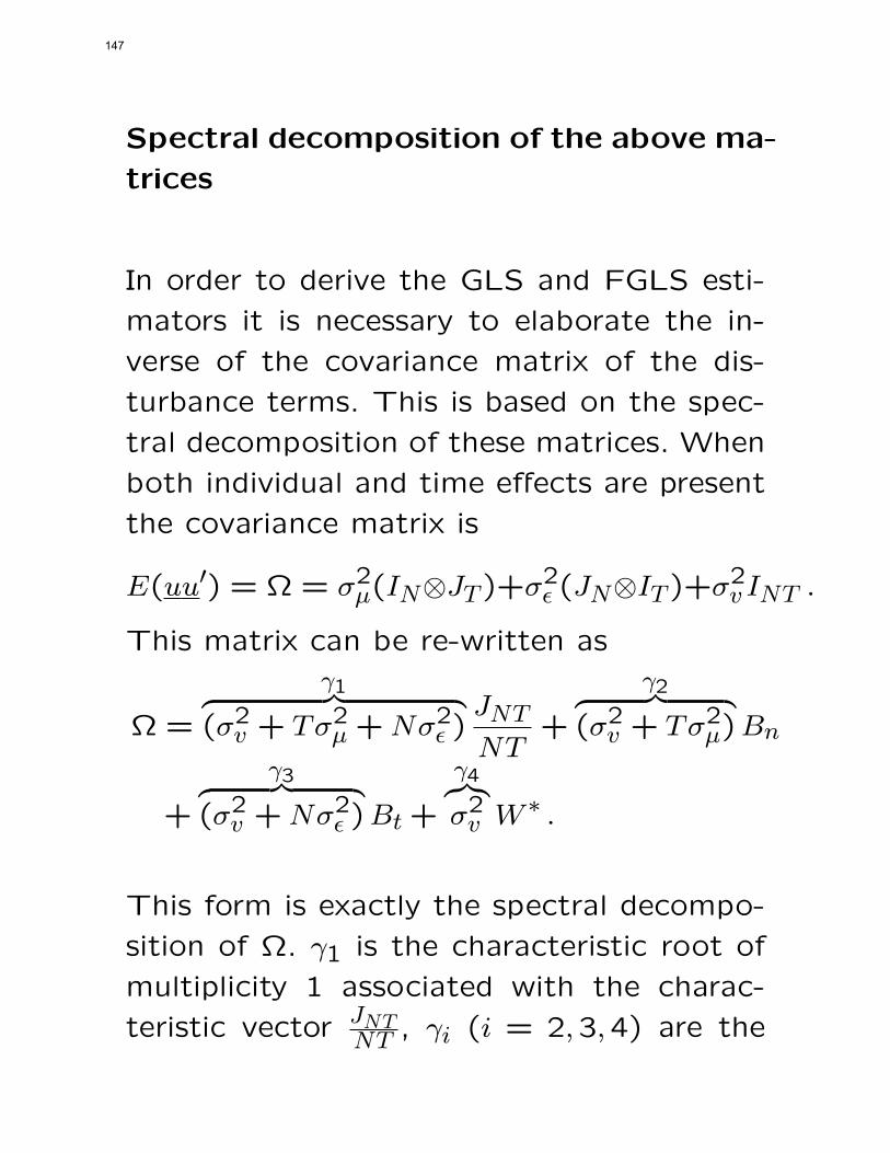
Spectral decomposition of the above ma-
trices
In order to derive the GLS and FGLS esti-
mators it is necessary to elaborate the in-
verse of the covariance matrix of the dis-
turbance terms. This is based on the spec-
tral decomposition of these matrices. When
both individual and time effects are present
the covariance matrix is
E(uu′) = Ω = σ2µ(IN⊗JT )+σ2ϵ (JN⊗IT )+σ2v INT .
This matrix can be re-written as
Ω =
γ1︷ ︸︸ ︷(σ2v + Tσ2µ +Nσ2ϵ )
JNT
NT+
γ2︷ ︸︸ ︷(σ2v + Tσ2µ)Bn
+
γ3︷ ︸︸ ︷(σ2v +Nσ2ϵ )Bt +
γ4︷︸︸︷σ2v W ∗ .
This form is exactly the spectral decompo-
sition of Ω. γ1 is the characteristic root of
multiplicity 1 associated with the charac-
teristic vector JNTNT , γi (i = 2,3,4) are the
147

characteristic roots of N − 1, T − 1, and
(N−1)(T −1) multiplicity respectively asso-
ciated with the characteristic vectors of the
matrices Bn, Bt, and W ∗. This means that
every power α of Ω can be written as
Ωα = γα1JNT
NT+ γα2Bn + γα3Bt + γα4W
∗ ,
so for instance its inverse is
Ω−1 = γ−11
JNT
NT+ γ−1
2 Bn + γ−13 Bt + γ−1
4 W ∗ .
Similarly the spectral decomposition of the
covariance matrix of the error components
model with only individual effects is
E(uu′) =
γ∗1︷︸︸︷σ2v Wn +
γ∗2︷ ︸︸ ︷(σ2v + Tσ2µ)Bn = Ω .
This means that any power of Ω can be
elaborated as
Ωα = γ∗α1 Wn + γ∗α2 Bn .
148

Estimation methods
1. OLS estimation
A “natural” estimator of the error compo-nents regression model is the OLS estima-tor. It is obvious that it is unbiased for bothmodels with only individual effects, and mod-els with individual and time effects. It has anormal distribution and its covariance ma-trix is
V (βOLS
) = (X ′X)−1X ′ΩX(X ′X)−1 .
We may need the OLS estimator for onlythe regression coefficients of the model(withoutthe constant term)
βOLS
= (X ′T ∗X)−1X ′T ∗y
and the covariance matrix in this case is
V (βOLS
) = (X ′T ∗X)−1X ′T ∗ΩT ∗X(X ′T ∗X)−1 .
After these evident small sample propertiesthe large sample properties have to be anal-ysed. Let us start with the model containingonly individual effects.
149

Model with Individual Effects
Assume that
H∗1 : lim
N&T→∞1
NTX ′BnX = BXX
is a positive definite matrix.
H∗2 : lim
N&T→∞1
NTX ′WnX = WXX
is also a positive definite matrix. Assump-tion H∗
2 implies that the estimated model(and therefore X) does not contain the con-stant term. When this term is present it isnecessary to assume that
plimN&T→∞
(1/NT )X ′T ∗X
and
plimN&T→∞
(1/NT )X ′BnX
are positive definite matrices. Then the OLSestimator is consistent.
(Conditions H∗1. and H∗
2. imply that
limN&T→∞
1
NTX ′X
is also a positive definite matrix.)
150

Under these assumptions the OLS estima-
tor is consistent when both N and T → ∞[The case in which both N and T → ∞ is
called asymptotic, when only N → ∞ it is
called semi–asymptotic.] . Unfortunately the
asymptotic covariance matrix of the OLS
estimator in this case is not finite: [This
reflects the fact that even asymptotically
(N&T → ∞), the covariance matrix V (βOLS−β) goes to zero at the speed 1/N . → Nor-
malization problem!]
V
(√NT (βOLS − β)
)=
=NT
(X ′X
NT
)−1X ′ΩX
N2T2
(X ′X
NT
)−1
=
(X ′X
NT
)−1X ′ΩX
NT
(X ′X
NT
)−1
.
151

The problem is that limN&T→∞X ′ΩXNT is not
finite, because
limN&T→∞
(σ2v + Tσ2µ)X′BnX
NT
is not finite due to the T factor.
If we now focus our attention on the semi–
asymptotic case, it can be shown under as-
sumptions
H∗3: limN→∞
1NX ′BnX = BXX is a positive
definite matrix, and
H∗4: limN→∞
1NX ′WnX = WXX is a positive
definite matrix, the OLS estimator is con-
sistent (N → ∞) and its asymptotic distri-
bution√N(β
OLS− β) is
N(0 , σ2µ(BXX+WXX)−1BXX(BXX+WXX)−1
).
152

Model with Individual and Time Effects
Under similar conditions than above the N
and T → ∞ the OLS estimator is consis-tent, but unfortunately just as in the previ-ous model its asymptotic covariance matrixis not finite. In the semi–asymptotic casethe OLS estimator is no longer consistent,even if we suppose that both
H∗5 : lim
N→∞1
NX ′X = T ∗
XX
and
H∗6 : lim
N→∞1
NX ′W ∗X = W ∗
XX
are positive definite matrices.
To show this, we start from the covariancematrix
Ω = σ2µTBn + σ2εNBt + σ2v INT .
The covariance matrix of the OLS estimatoris
V (β) = (X ′X)−1X ′ΩX(X ′X)−1 ,
153

then
limN→∞
V (β) = T ∗−1XX lim
N→∞X ′ΩX
N2T ∗−1XX ,
so we can see that the analysed limit is not
equal to zero i.e., the OLS estimator is in-
consistent. The same thing happens if we
want to estimate a model with only indi-
vidual effects, or a model with individual
and time effects, when N is finite and only
T → ∞, or also when only time effects are
present and T is finite. This is due to the un-
usual fact that in these cases there are a lim-
ited number of observations for a given ran-
dom variable even if the sample size grows
to infinity.
Of course, in none of the cases is the OLS
estimator efficient, because it neglects the
information present in the covariance matrix
of the error term.
154

2. GLS estimation
The GLS estimator is
βGLS = (X ′Ω−1X)−1X ′Ω−1y .
If we want to use this, we need the inverseof the covariance matrix Ω. Starting fromthe covariance matrices of the error com-ponents models and using their spectral de-composition
for the model with individual effects only,
Ω−1 =1
σ2vWn +
1
(σ2v + Tσ2µ)Bn ,
and, for the model with both individual andtime effects,
Ω−1 =1
σ2v + Tσ2µ +Nσ2ε
JNT
NT+
1
σ2v + Tσ2µBn+
+1
σ2v +Nσ2εBt +
1
σ2vW ∗ .
Using these inverse matrices, the GLS esti-mators are
βGLS = (X ′WnX+θX ′BnX)−1(X ′Wny+θX ′Bny) ,
155
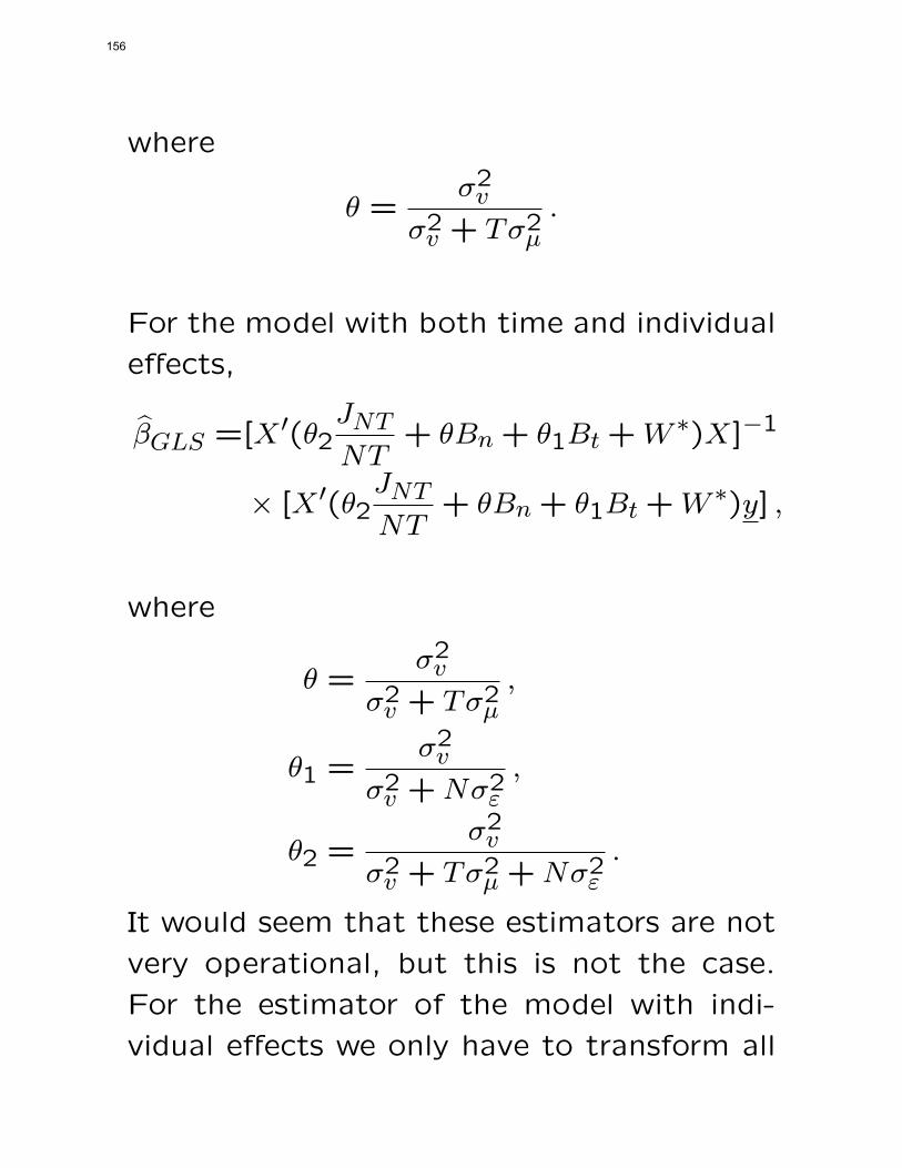
where
θ =σ2v
σ2v + Tσ2µ.
For the model with both time and individual
effects,
βGLS =[X ′(θ2JNT
NT+ θBn + θ1Bt +W ∗)X]−1
× [X ′(θ2JNT
NT+ θBn + θ1Bt +W ∗)y] ,
where
θ =σ2v
σ2v + Tσ2µ,
θ1 =σ2v
σ2v +Nσ2ε,
θ2 =σ2v
σ2v + Tσ2µ +Nσ2ε.
It would seem that these estimators are not
very operational, but this is not the case.
For the estimator of the model with indi-
vidual effects we only have to transform all
156
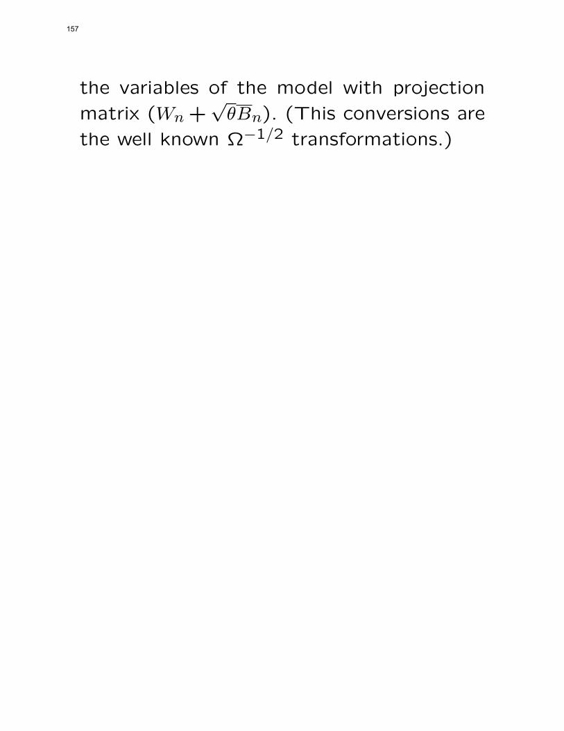
the variables of the model with projection
matrix (Wn +√θBn). (This conversions are
the well known Ω−1/2 transformations.)
157

The effects of these projections can be shown,
for example, on the vector y:
(Wn +√θBn)y = [yit − (1−
√θ)yi]
We can proceed likewise for the models with
both individual and time effects (see the
reader).
Summing up, the GLS estimators are useful
to estimate the error components models if
the Θ, Θ1 and Θ2 parameters are known.
We only have to perform appropriate trans-
formations on all the variables of the model
and then use the OLS to estimate the trans-
formed model.
158

Now it is time to analyse the properties ofthe GLS estimators.
Properties of the GLS Estimator for theModel with Only Individual Effects.
It is obvious from classical theory that theGLS estimator is unbiased and (from theGauss–Markov theorem) it is the best linearunbiased estimator (BLUE) of the param-eters (The GLS estimators can be consid-ered the optimal linear combinations of thewithin and between estimators.)
Its covariance matrix is
V (βGLS
) = (X ′Ω−1X)−1
= σ2v(X ′WnX +
σ2vσ2v + Tσ2µ
X ′BnX)−1
.
Under the normality assumptions the GLSestimator has a normal distribution:
βGLS
∼ N(β , σ2v
(X ′WnX+
σ2vσ2v + Tσ2µ
X ′BnX)−1
).
159

Now let us focus our attention on the large
sample properties. Under hypotheses made
earlier if T and N → ∞ is consistent. This
can be shown as follows:
limN&T→∞
V (βGLS
) =
= limN&T→∞
σ2v(NT
X ′WnX
NT+
NTσ2v
σ2v + Tσ2µ
X ′BnX
NT
)−1= 0 .
Moreover the asymptotic distribution of the
GLS estimator is√NT (β
GLS− β)
A∼N (0, σ2vW−1XX) .
The semi-asymptotic case (N → ∞ T finite)
and the model with individual and time ef-
fects can be dealt with in a similar way (see
reader).
In general we do not know the variance com-
ponents, so they must be estimated from
the sample and the GLS cannot be applied
directly.
160
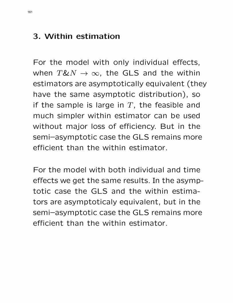
3. Within estimation
For the model with only individual effects,
when T&N → ∞, the GLS and the within
estimators are asymptotically equivalent (they
have the same asymptotic distribution), so
if the sample is large in T , the feasible and
much simpler within estimator can be used
without major loss of efficiency. But in the
semi–asymptotic case the GLS remains more
efficient than the within estimator.
For the model with both individual and time
effects we get the same results. In the asymp-
totic case the GLS and the within estima-
tors are asymptoticaly equivalent, but in the
semi–asymptotic case the GLS remains more
efficient than the within estimator.
161

Estimators for the Variance Components
For the model with individual effects only:
E(u2it) = σ2µ + σ2v ,
E
(1T
∑t
uit)2
= σ2µ +1
Tσ2v ,
and the estimates of these expected values
are
E(uit)2 ⇒
∑i∑
t u2it
NT −K
E
(1T
∑t
uit)2
⇒∑
i1T (∑
t uit)2
N −K,
where uit can be for example the OLS, the
within or any other residual obtained by the
consistent estimation of the model. Then
the estimates of the variance components
162
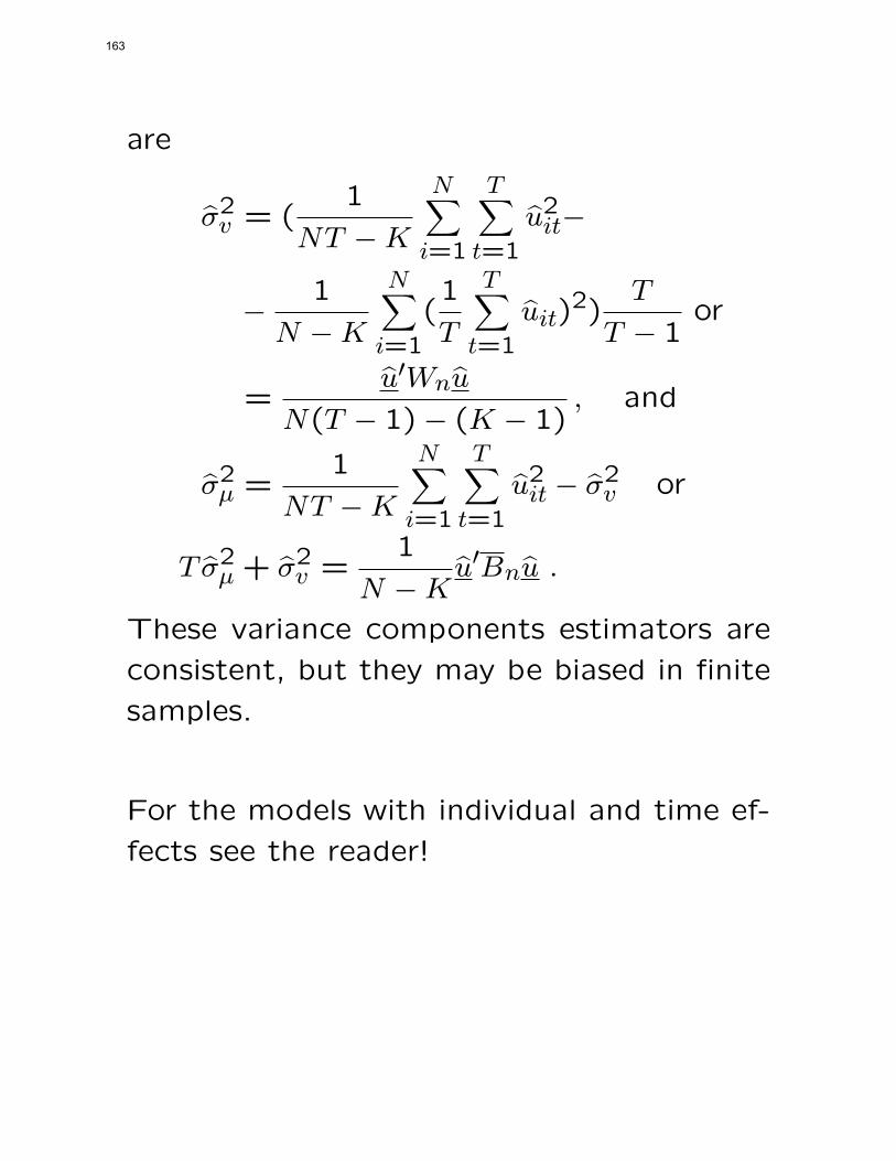
are
σ2v = (1
NT −K
N∑i=1
T∑t=1
u2it−
−1
N −K
N∑i=1
(1
T
T∑t=1
uit)2)
T
T − 1or
=u′Wnu
N(T − 1)− (K − 1), and
σ2µ =1
NT −K
N∑i=1
T∑t=1
u2it − σ2v or
T σ2µ + σ2v =1
N −Ku′Bnu .
These variance components estimators are
consistent, but they may be biased in finite
samples.
For the models with individual and time ef-
fects see the reader!
163

Topic : PD3
Linear Panel Data Models Summaryand Dynamic Models
164

Linear Panel Data Estimators – Sum-
mary
1. FE(1) model – WITHIN estimator: i)
Separability, ii) restrictions on the indi-
vidual effects and the constant term
• consistent for β (N&T → ∞ and N →∞)
• not consistent for α (if N → ∞)
2. FE(2) model – WITHIN estimator: i)
Separability, ii) restrictions on the indi-
vidual and time effects
• consistent for β (N&T → ∞ and N →∞)
• not consistent for α and/or λ if that
dimension goes to infinity.
165

3. RE(1) model
• OLS – i) not finite asympt. cov ma-
trix but consistent when N&T → ∞;
ii) consistent and finite asympt. cov
matrix when N → ∞.
• GLS – i) consistent and finite asympt.
cov. matrix when N → ∞; ii) consis-
tent and asympt. cov matrix = Within
asympt. cov. matrix when N&T →∞;
• Within – i) N&T → ∞ GLS and Within
estimators are equivalent; ii) N → ∞consitent, asympt. cov. matrix finite,
but GLS more efficient.
166

4. RE(2) model
• OLS – not finite asympt. cov matrix
but consistent when N&T → ∞; but
not consistent when N → ∞.
• GLS – i) consistent and finite asympt.
cov. matrix when N → ∞; ii) consis-
tent and asympt. cov matrix = Within
asympt. cov. matrix when N&T →∞;
• Within – i) N&T → ∞ GLS and Within
estimators are equivalent; ii) N → ∞consitent, asympt. cov. matrix finite,
but GLS more efficient.
167

Dynamic Linear Panel Data Models
The autoregressive fixed effects model canbe written as:
yit = δyi,t−1 + x′itβ + αi + uit .
We assume that the disturbances are uncor-related with the explanatory variables, arenot serially correlated and are homoscedas-tic. Stacking all observations over individu-als and time periods, we get, in matrix form,the following model:
y = δy−1 +Xβ +DNα+ u
with
y =
y11...
y1T...
yNT
, y−1 =
y10...
y1,T−1...
yN,T−1
,
X =
x(1)11 . . . x
(k)11... . . . ...
x(1)1T . . . x
(k)1T... . . . ...
x(1)NT . . . x
(k)NT
168

The Inconsistency of the LSDV (Within)
Estimator When T is Finite
Although the disturbances of the model are
assumed to be i.i.d., this model cannot be
consistently estimated by OLS (or Within
which in this case is the same) as long as
the number of periods is finite. We have
seen that the estimation of coefficients δ
and β can be done by applying OLS to the
following transformed model:
Wny = Wny−1δ +WnXβ +Wnu ,
Then, the OLS estimator of δ and β can be
written as(δ
β
)=
(y′−1Wny−1 y′−1WnX
X ′Wny−1 X ′WnX
)−1(y′−1Wny
X ′Wny
)since Wn is a symmetric idempotent matrix.
169

When N → ∞, one can write:
plimN→∞
(δ
β
)=
(δβ
)+
+
plimN→∞
1NT y
′−1Wny−1 plim
N→∞1
NT y′−1WnX
plimN→∞
1NTX
′Wny−1 plimN→∞
1NTX
′WnX
−1
×
plimN→∞
1NT y
′−1Wnu
plimN→∞
1NTX
′Wnu
.
The inconsistency of this estimator rests on
the fact that, given the assumption about
the disturbances, one has
plimN→∞
1
NTX ′Wnu = 0
170

but, on the other hand,
plimN→∞
1
NTy′−1Wnu =
= plimN→∞
1
NT
∑i
∑t
(yi,t−1 − yi−1)(uit − ui)
= E(1T
∑t
(yi,t−1 − yi−1)(uit − ui))
= −1
T2
T − 1− Tδ + δT
(1− δ)2σ2u = 0 .
Then, as long as the number of periods is
kept fixed, the OLS estimator of an autore-
gressive fixed effects model is not consis-
tent. This semi–inconsistency is due to the
asymptotic correlation that exists between
(yi,t−1 − yi−1) and (uit − ui) when N → ∞ :
though yi,t−1, and uit are uncorrelated, their
respective individual means are correlated
with each other, with uit and with yi,t−1, and
the sum of those three covariances does not
vanish.
171

As it is clear from above, when N & T → ∞,
this estimator is consistent since (we need
to assume |δ| < 1.)
plimN&T→∞
1
NTy′−1Wnu = 0 .
Hence, if the number of periods in the sam-
ple is large enough, the asymptotic bias of
this estimator is likely to be rather small.
Nevertheless, frequently panel data sets that
one has to deal with contain observations
over only a few time–periods. Therefore,
one has to look for estimation methods that
are consistent when T is fixed.
172

Instrumental Variables (IV) Estimation
The semi–inconsistency of the OLS estima-
tor of an autoregressive fixed effects model
is due to the asymptotic correlation between
the lagged endogenous variable and the dis-
turbances. A traditional way to tackle this
kind of problem is to use an instrumental
variables estimation method. There are two
main ways to deal with the problem: i) in-
strument the model in levels, or ii) instru-
ment the model in first differences. (We can
also use GMM of course!) Let us see how
this second works.
Let us write the model in first differences:
∆y = δ∆y−1 +∆X ′β +∆u
that is,
yit − yi,t−1 = δ(yi,t−1 − yi,t−2)+
+ (x′it − x′i,t−1)β + uit − ui,t−1
The OLS estimator is not consistent for
this model as correlation exists between the
173

lagged endogenous variable and the distur-
bances. However, it is possible to tackle this
problem by using IV. For example, Anderson–
Hsiao(1982) proposed to use as instrumen-
tal variables either
Z1it =(yi,t−2, x
′it − x′i,t−1
)or
Z2it =(yi,t−2 − yi,t−3,, x
′it − x′i,t−1
)Obviously, the variables yi,t−2 and ∆yi,t−2 =
yi,t−2−yi,t−3 are valid instruments since they
are correlated with yi,t−1−yi,t−2, but are un-
correlated with the disturbance uit − ui,t−1,
given the non–autocorrelation of the uit’s.
There are many other IVs proposed in the
literature.
174
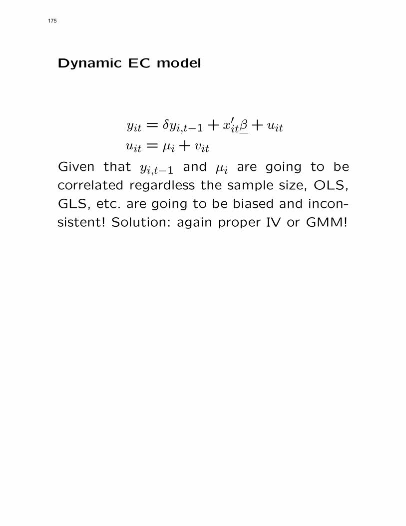
Dynamic EC model
yit = δyi,t−1 + x′itβ + uit
uit = µi + vit
Given that yi,t−1 and µi are going to be
correlated regardless the sample size, OLS,
GLS, etc. are going to be biased and incon-
sistent! Solution: again proper IV or GMM!
175

Topic : PD4
Linear Panel Data Models:Poolability and Extensions
176
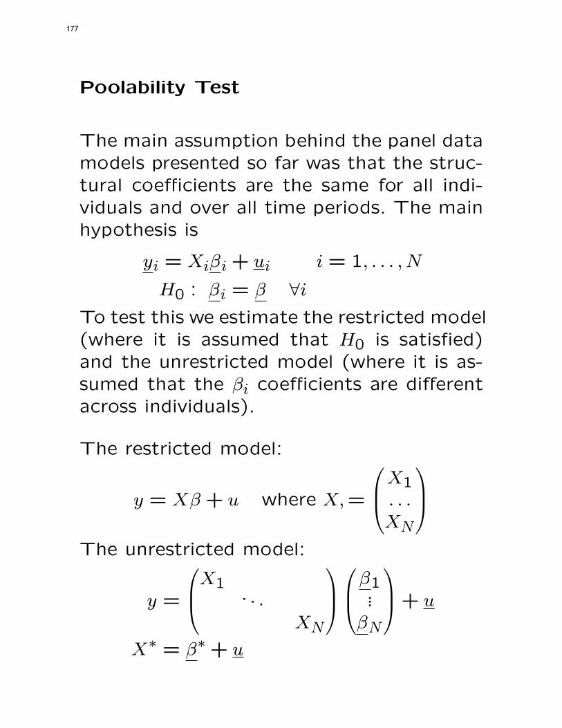
Poolability Test
The main assumption behind the panel datamodels presented so far was that the struc-tural coefficients are the same for all indi-viduals and over all time periods. The mainhypothesis is
yi = Xiβi + ui i = 1, . . . , N
H0 : βi = β ∀iTo test this we estimate the restricted model(where it is assumed that H0 is satisfied)and the unrestricted model (where it is as-sumed that the βi coefficients are differentacross individuals).
The restricted model:
y = Xβ + u where X,=
X1. . .XN
The unrestricted model:
y =
X1. . .
XN
β1
...βN
+ u
X∗ = β∗ + u
177

Taking the residuals (easing the notation:
no underlining):
y = XβOLS + e
e = My, M = INT −X(X ′X)−1X ′
and for the unrestricted case
yi = XiβOLS + ei
ei = Miyi, Mi = IT −Xi(X′iXi)
−1X ′i
M∗ =
M1. . .
MN
y = X∗β∗ + e∗
e∗ = M∗y
Then the test statistic is
F =(e′e− e∗
′e∗)/tr(M)− tr(M∗)
e∗′e∗/tr(M∗)
where tr stands for trace, tr(M)− tr(M∗) =
(N − 1)K, tr(M∗) = N(T − K), which are
the DF of the F test! Please note: this is in
fact a generalized Chow test!
There are other, but similar in concept tests.
178

Unbalanced Panels
1. Rotating panels; 2. Missing at rando/not
random
Example: For the FE model with individual
effects the Within transformation (yit − yi)
now has
yi =
∑Tit=1 yit
Ti
where Ti is the number of time periods ob-
served for individual i. The corresponding
within transformation is
Wn = diag[(IT1 − JT1/T1), . . . , (ITN − JTN/TN)
]which is to be used to transform the model.
With time effects: much more complicated.
179

Varying Coefficients
Fixed coefficients:y1...
yN
=
Z1 0.. .
ZN
γ1
...γN
+Xβ + u
y = Zγ +Xβ + u
We need two projector matrices:
PZ = [INT − Z′(Z′Z)−1Z]
PX = [INT −X ′(X ′X)−1X]
Then the transformed model
PZy = PZZγ + PZXβ + PZu
can be estimated by OLS as PZZ = 0, which
gives
β = (X ′PZx)−1X ′PZy
which is N and T consistent as well.
180
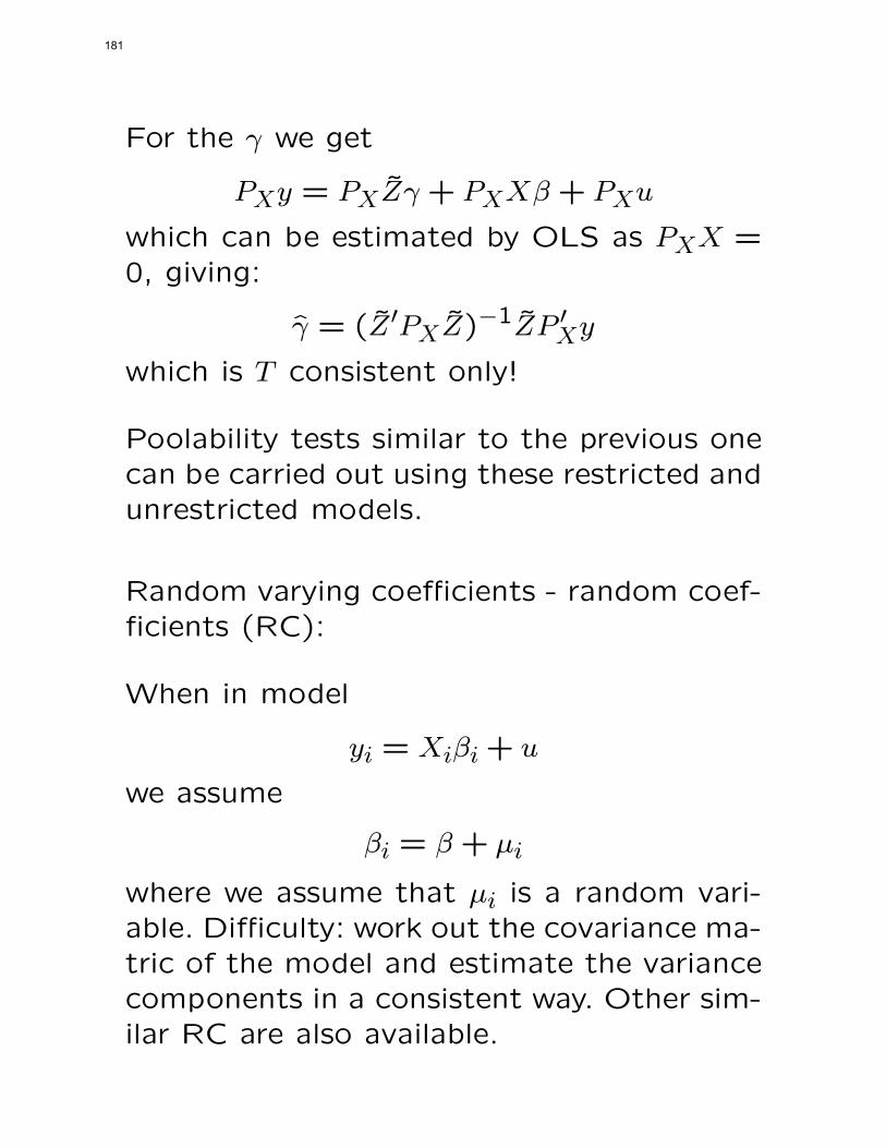
For the γ we get
PXy = PXZγ + PXXβ + PXu
which can be estimated by OLS as PXX =0, giving:
γ = (Z′PXZ)−1ZP ′Xy
which is T consistent only!
Poolability tests similar to the previous onecan be carried out using these restricted andunrestricted models.
Random varying coefficients - random coef-ficients (RC):
When in model
yi = Xiβi + u
we assume
βi = β + µi
where we assume that µi is a random vari-able. Difficulty: work out the covariance ma-tric of the model and estimate the variancecomponents in a consistent way. Other sim-ilar RC are also available.
181
Non-linear models
Main difficulties:FE models: Non-separability → The incon-sistency in the estimation of the Fixed Ef-fects is carried over to the estimation of thestructural parameters β.RE models: Misspecified heterogeneity → Bi-ased and inconsistent parameter estimates.
EXAMPLES:
Probit FE model:
yit = F (β′xit + αi) + ϵit
The estimation of β and αi-s are linked. SoMLE consistent only if T → ∞ and N fixedfinite, or N&T → ∞ but N/T → 0.
Similarly, for the Logit model, the Log L is:
lnL =∑∑
ln[1 + exp(β′xit + αi)]+
+∑∑
yit(β′xit + αi)
182

similarly as for the Probit, plimN→∞ βML =β!
RE models:
To take into account the individual random
effect (or heterogeneity factor) µi we need
to specify its distribution:
µi ∼ π(ν, γ)
then
f(yit/xit, µ, β, γ) =
=∫
f(yit, x′itβ + µ)π(µ, γ)dµ
that is we integrate out the µi individual
effects. (There are N integrals in the above
formula!)
EXAMPLE: Probit model with normal µi
P (yit = 1/xit, µi) = Φ(x′itβ + µi)
if µ ∼ N(0, σ2µ), then
P (yit = 1/xit) =∫
Φ(x′itβ + µ)1
σϕ(
µ
σµ)dµ
183

Duration models
Variable of interest → the duration of an
event, the length of time that elapses (du-
ration) from the beginning of some event
until its end (or the end of the measure-
ment). E.g., unemployment duration, dura-
tion of strikes, etc...
Observations → cross sections (panels in
fact) of durations. Duration we observe are
called spells.
Problem of censoring → at the end of mea-
surements many spells are censored (e.g.,
may be unemployed beyond the measure-
ment period).
Problem of time continuity → Explanatory
variables of a model may take different val-
ues of a spell. E.g., employment is a func-
tion of education, but this may change over
an unemployment spell if this time is used
184

for education (these are called in this con-
text time varying covariates).
BACKGROUND
Assume that r.v T (sorry, but this is the
usual notation here, please do not confuse
it with the time period length!) has a con-
tinuous probability distribution f(t) and t is
a realization of T .The cumulative then is:
F (t) =∫ t
0f(s)ds = Prob(T ≤ t)
We are usually interested in how long does
a spell last → survival function:
S(t) = 1− F (t) = Prob(T ≥ t)
Question: Assuming a spell has lasted up to
time t, what is the probability that it will end
in the next ∆ time interval. This is called
Hazard rate:
l(t,∆) = Prob(t ≤ T ≤ t+∆/T ≥ t)
185

Then the rate at which spells are completed
after a duration t is
λt = lim∆→0
Prob(t ≤ T ≤ t+∆/T ≥ t)
∆
= lim∆→0
F (t+∆)− F (t)
∆S(t)
=f(t)
S(t)
Frequent model simplifying assumptions:
Hazard rate does not change over time: λ(t) =
λ.
Or λ(t) = α+ βt.
Or: positive duration dependence → the like-
lihood of the end of a spell at t is conditional
upon the duration up to t.
Estimation by ML (with θ parameters):
lnL =∑
uncensored observations
ln f(t/θ)+
+∑
censored observations
lnS(t/θ)
186

The most popular (simple) model formula-
tion is where the durations are exponentially
distributed:
f(yit/zit, β) =
λit exp (−λityit) if yit > 0
0
with λit = exp(z′itβ).
The same with random individual hetero-
geneity:
yit = (λ+ µi) exp[−(λ+ µi)yit]
187

Topic : PD5
Short Introduction toMulti-dimensional Panel Models
188

A typical 3D panel model looks like this:
yijt = x′ijtβ + uijt
i = 1, . . . N1, j = 1, . . . , N2 t = 1, . . . , T.
Examples of such 3D data: Matched employer-
employee, matched doctor-patient, trade, etc....
Higher dimensional data: E.g., with more
detailed geographical location → xijst trade
from country i in county j to country s in
time t. Another example: Priceijst price of
a good i, in a supermarket j, in location s,
at time t (barcode data).
Main features:
• Heterogeneity: FE and RE, but the avail-
able formulation much larger due to the
interaction effects.
• Incomplete/unbalanced data
189

• several different “semi–asymptotics”
• Potentially very large data sets
• Right hand side “index deficit”
190

Fixed Effects Models
In general that the index sets i ∈ 1, . . . , N1and j ∈ 1, . . . , N2 are (completely or par-
tially) different. When dealing with economic
flows, such as trade, capital, investment (FDI),
etc., there is some kind of reciprocity, in
such cases it is assumed that N1 = N2 =
N . The main question is how to formal-
ize the individual and time heterogeneity –
in our case, fixed effects. In standard two-
dimensional panels, there are only two ef-
fects, individual and time, so in principle
22 model specifications are possible (if we
also count the model with no fixed effects).
The situation is fundamentally different in
three-dimensions. Strikingly, the 6 unique
fixed effects formulations enable a great va-
riety, precisely 26, of possible model speci-
fications. Of course, only a subset of these
are used, or make sense empirically.
191
The most relevant models specifications are:
yijt = x′ijtβ + αi + γj + λt + εijt , (2)
where the αi, γj, and λt parameters are the
individual and time-specific fixed effects. One
of the most complex ones with multiple in-
teraction effect is:
yijt = x′ijtβ + γij + αit + α∗jt + εijt ,
In matrix form
y = Xβ +Dπ + ε
with y and X being the vector and matrix
of the dependent and explanatory variables
(covariates) respectively of size (N1N2T ×1) and (N1N2T × K), β being the vector
of the slope parameters of size (K × 1), π
the composite fixed effects parameters, D
the matrix of dummy variables, and finally,
ε the vector of the disturbance terms.
192

For model (2) π = (α′ γ′ λ′)′ with α′ =
(α1, . . . , αN1), γ′ = (γ1, . . . , γN2
) and λ′ =
(λ1, . . . , λT ) and the appropriate D matrices
are for the above two models:((IN1
⊗ lN2T ), (lN1⊗ IN2
⊗ lT ), (lN1N2⊗ IT )
)and((IN1N2
⊗ lT ), (IN1⊗ lN2
⊗ IT ), (lN1⊗ IN2T )
)
The models (β parameters) can be estimated
(for complete data) with generalized Within
transformations of the form
[I − (IN1⊗ JN2T )− (JN1
⊗ IN2⊗ JT )−
− (JN1N2⊗ IT ) + 2JN1N2T ]
with DF = N1N2T −N1−N2−T +1−K and
[I − (IN1⊗ JN2
⊗ IT )− (JN1⊗ IN2T )−
− (IN1N2⊗ JT ) + (JN1N2
⊗ IT )+
+ (JN1⊗ IN2
⊗ JT ) + (IN1⊗ JN2T )− JN1N2T ]
with DF = (N1−1)(N2−1)(T −1)−K and
J denotes the normalized J (each element
is divided by the number in the subscript).
193

Beware: right hand side index deficit and
fixed effects formulations should be “coor-
dinated” for identification purposes. For ex-
ample in a 3D model if we have xit type ex-
planatory variables, we should not have αit
type fixed effects, etc. as they cannot be
identified separately (the respective within
transformation would wipe both out).
194

Supporting materials for the Lecture Notes
Topics and Reading
195
Topic 0: Assumed Background
• Classical linear regression model, assumptions
• How to derive the OLS and GLS estimators
• OLS finite sample properties
• GLS finite sample properties
• Where are all the above assumptions used
• Model wit AR(1) disturbances and heteroscedasticity, related tests
• Basic hypothesis testing (null and alternative, significance level, criticalvalue)
• Basic tests in the Classical linear regression model (t, F , R2, het-eroscedasticity and autocorrelation, etc.)
REFERENCES:
Bruce E. Hansen: Econometrics (2019), 12-27, 39-41, 63-74, 75-82, 101-106, 108-111, 113-117, 100-106, 147-151, 154-156.
William Greene: Econometric Analysis (6th edition, 2008), pp: 8-39, 43-63, 148-150, 154-173, 945-972, 974-975, 976-983, 987-1019, 1023-1032, 1034-1036.
Jeffrey Wooldridge: Introductory Econometrics (2003), 21-111, 116-153, 257-279
Russell Davidson and James MacKinnon: Econometric Theory andMethods (2004), pp. 1-30, 42-75, 100-103, 122-146.
William Griffiths, Carter Hill, and George Judge: Learning andPracticing Econometrics, 1993, pp.287-355, 431-444, 483-513, 514-579
Fumio Hayashi: Econometrics, 2000, pp. 3-44,
Further useful references:
Maxwell King: Serial Correlation, in Baltagi: A Companion to The-oretical Econometrics, 2001, pp. 62-81.
William E. Griffiths: Heteroscedasticity, in Baltagi: A Companion toTheoretical Econometrics, 2001, pp. 82-93.
196

Topics 1-2
• Parametric, non-parametric models, conditional distributions
• Identification
• Elements of Asymptotic Theory:
• OLS and GLS estimators asymptotic properties
• FGLS estimator asymptotic properties
REFERENCES:
Main reading
Harris-Matyas: Handout/Reader: pp. 1-23, 31-36Bruce E. Hansen: Econometrics (2019), 171-176, 177-180, 182-183, 186-
187, 212-217, 222-224
Additional references
Benedikt Potscher and Ingmar Prucha: Basic Elements of Asymp-totic Theory, in Baltagi, A Companion to Theoretical Econometrics, 2001,pp.201-229.
Franco Peracchi: Econometrics, 2001, pp. 1-47, 657-670William Greene: Econometric Analysis (6th Edition, 2008) pp: 63-76,
151-156, 1038-1061Jeffrey Wooldridge: Econometric Analysis of Cross Section and Panel
Data, 2002, pp. 13-24, 29-31, 35-42, 51-55
Further references
Brendan McCabe and Andrew Tremayne: Elements of ModernAsymptotic Theory with Statistical Applications, Manchester University Press,1993, Chapters 3 and 4.
Russell Davidson and James G. MacKinnon: Estimation and In-ference in Econometrics, Oxford University Press, 1993, pp. 99-139.
Ron Mittelhammer, George Judge and Douglas Miller: Econo-metric Foundations, 2000, pp.13-32.
197

Topics 3-4
• Maximum likelihood estimation
• Concentrated maximum likelihood
• Quasi (Pseudo) maximum likelihood estimation
• Extremum estimation
REFERENCES:
Main reading
William Greene: Econometric Analysis (6th Edition, 2008) pp: 484-496Russell Davidson and James MacKinnon: Econometric Theory and
Methods (2004), pp: 399-420Aris Spanos: Statistical Foundations of Econometric Modelling, Cam-
bridge University Press (first edition 1986): pp: 257-284Ron Mittelhammer, George Judge and Douglas Miller: Econo-
metric Foundations, 2000, pp. 35-53, 133-156, 245-255Fumio Hayashi: Econometrics, 2000, 445-465, 469-478
Additional suggested/recommended (but not compulsory!) reading
Jeffrey Wooldridge: Econometric Analysis of Cross Section and PanelData, 2002, pp. 389-397, 401-408, 648-656.
Christian Gourieroux and Alain Monfort: Statistics and Econo-metric Models, Cambridge University Press, 1996, v1, pp. 234-248, v2, pp.276-282.
Brendan McCabe and Andrew Tremayne: Elements of ModernAsymptotic Theory with Statistical Applications, Manchester Uni. Press,1993: pp: 129-154
Franco Peracchi: Econometrics, 2001, pp. 139-172Fernandez-Villaverde et al.: Convergence Properties of the Likelihood
of Computed Dynamic Models, Econometrica, 2006, pp. 93-119Daniel Ackerberg et al.: Comment on ”Convergence Properties of the
Likelihood of Computed Dynamic Models”, Econometrica, 2009, pp. 2009-2017.
198
Topic 5
• Empirical Likelihood
• Monte-Carlo methods (simulation)
• Bootstrapping (re-sampling)
REFERENCES:
Ron Mittelhammer, George Judge and Douglas Miller: Econo-metric Foundations (2000), pp. 281-312, 713-730
Bruce E. Hansen: Econometrics (2018), 479-482.Russell Davidson and James G. MacKinnon: Estimation and In-
ference in Econometrics, Oxford University Press, 1993, pp. 731-769William Greene: Econometric Analysis (6th Edition, 2008) (meager):
pp. 573-576, 584-589, 596-598Colin Cameron and Pravin Trivedi: Microeconometrics, Cambridge
Univ Press 2005, pp: 251-257, 357-373
Additional Reading:
Art B. Owen: Empirical Likelihood, Chapman & Hall, 2001
199

Topic 6
• Hypothesis testing in econometrics
REFERENCES:
Bruce E. Hansen: Econometrics (2019), 139-159, 230-233, 236-237, 276-293, 301-305.
William Greene: Econometric Analysis (6th Edition, 2008): pp: 81-82,92-96, 133-146, 298-300, 498-507, 518-522.
Aris Spanos: Probability Theory and Statistical Inference, 1999, pp.681-728.
Ron Mittelhammer, George Judge and Douglas Miller: Econo-metric Foundations, 2000, pp. 63-72, 105-111, 114-117, 118-120, 217-219
Colin Cameron and Pravin Trivedi: Microeconometrics, CambridgeUniv Press 2005, pp: 223-256
Russell Davidson and James G. MacKinnon: Estimation and In-ference in Econometrics, Oxford University Press, 1993, pp. 435-479.
Aris Spanos: Statistical Foundations of Econometrics Modelling, pp.285-306, 328-338, 392-402, 589-599.
James Davidson: Econometric Theory, 2000, pp. 283-307Christian Gourieroux and Alain Monfort: Statistics and Economet-
ric Models, Vol 2, 1995, pp.1-324
200

Topics 7-8
• Instrumental variables estimation (IV)
• Generalised Method of Moments estimation (GMM)
• Testing for overidentifying restrictions, Conditional Moments Tests,Hausman Test.
REFERENCES:
Bruce E. Hansen: Econometrics (2019): 388-393, 396-399, 401-403, 428-438, 442-448.
David Harris, and Laszlo Matyas: Asymptotics for Estimation andInference; handout; pp. 45-51.
Laszlo Matyas (ed): Generalized Method of Moments Estimation, Cam-bridge University Press, 1999, Chapter 1, pp. 3-30. (main reference)
Further reading
Colin Cameron and Pravin Trivedi: Microeconometrics, CambridgeUniv Press 2005, pp: 95-111, 166-212, 260-274
Joshua D. Angris and Alan B. Krueger: Instrumental Variables andthe Search for Identification. (Handout).
201
Topic 9
• Restricted estimation
• Mixed estimation
• Pre-test estimators
REFERENCES:
Bruce E. Hansen: Econometrics (2019): 251-259.William Greene: Econometric Analysis (4th Edition, 2000): pp: 338-
345.Russell Davidson and James G. MacKinnon: Estimation and In-
ference in Econometrics, Oxford University Press, 1993, pp. 16-24, 677-680Ron Mittelhammer, George Judge and Douglas Miller: Econo-
metric Foundations, 2000, pp. 80-82, 551-556, 500-508
and (a bit old but still the main reference in this area)
Thomas Fomby, Carter Hill and Stanley Johnson: Advanced Econo-metric Methods, Springer-Verlag, 1984, pp.80-108, 122-131
202

Topics 10
• Non-nested Model Selection
• Binary Choice Models and Multinomial Models
• Truncated and Censored models
• Sample Selectivity
REFERENCES:
Marno Verbeek: A Guide to Modern Econometrics, Wiley 2000, pp.177-223. (handout).
Jeff Wooldridge: Econometric Analysis of Cross Section and PanelData, 2002, pp. 453-472, 497-499, 517-529, 536-538, 551-566, 645-653, 685-695
William Greene: Econometric Analysis (5th Edition, 2003): pp: 663-689, 723-728, 756-768, 780-786.
AND (just as supplementary reading)
Russell Davidson and James G. MacKinnon: Estimation and Inferencein Econometrics, Oxford University Press, 1993, pp. 511-546
Colin Cameron and Pravin Trivedi: Microeconometrics, CambridgeUniv Press 2005, pp: 461-474, 476-479, 490-497, 529-544, 546-551
Patrick A. Puhani: The Heckman Correction for Sample Selection andits Critique, Journal of Economic Surveys,Vol.14, No. 1, 2002.
Additional reading only (but this is the main reference book in these topics)
Christian Gourieroux: Econometrics of Qualitative Dependent Vari-ables, Cambridge University Press, 2000 (a bit outdated, but still the mainreference book in this field), pp. 1-37, 72-106, 170-200, 270-281, 284-357.
203

Topic 11
• Linear models for panel data
• Dynamic models
• Selectivity
• Non-linear models for panel data
• Multi-dimensional panels
REFERENCES:
Matyas et al.: e.handout on the e.learning site; main reference.William Greene: Econometric Analysis (4th Edition, 2000): pp: 557-584Jeff Wooldridge: Econometric Analysis of Cross Section and Panel
Data, 2002, pp. 169-179, 247-291, 299-323, 401-409, 410-414, 482-495, 497-504, 538-544, 577-590, 668-676
Badi Baltagi: The Econometric Analysis of Panel Data (Wiley, 1995):pp:1-26, 47-76, 125-148, 169-196
Laszlo Matyas (ed): The Econometrics of Multi-dimensional Panels: pp.1-70
AND (as additional reading only)Laszlo Matyas and Patrick Sevestre: The Econometrics of Panel
Data (Kluwer Academic Publishers, 1992, 1996, 2008): Any chapter in Parts1 & 2 (this forms the basis of your handout)
Cheng Hsiao: Analysis of Panel Data (Cambridge, 1986), any part, abit outdated in some aspects.
Jeff Wooldridge: Econometric Analysis of Cross Section and PanelData, 2002, pp 603-614, 686-714
204


![Takeshi Amemiya-Advanced Econometrics[1]](https://img.pdfslide.us/doc/110x75/543b86b9afaf9fe7568b4999/takeshi-amemiya-advanced-econometrics1.jpg)