Embed Size (px)
Citation preview
INTERMEDIATE AND ADVANCEDECONOMETRICS
Problems and Solutions
Stanislav Anatolyev
February 7, 2002

2
Contents
I Problems 9
1 Asymptotic theory 111.1 Asymptotics of t-ratios . . . . . . . . . . . . . . . . . . . . . . . . . . . . . . . . . . . 111.2 Asymptotics with shrinking regressor . . . . . . . . . . . . . . . . . . . . . . . . . . . 111.3 Creeping bug on simplex . . . . . . . . . . . . . . . . . . . . . . . . . . . . . . . . . . 121.4 Asymptotics of rotated logarithms . . . . . . . . . . . . . . . . . . . . . . . . . . . . 121.5 Trended vs. differenced regression . . . . . . . . . . . . . . . . . . . . . . . . . . . . 121.6 Second-order Delta-Method . . . . . . . . . . . . . . . . . . . . . . . . . . . . . . . . 131.7 Brief and exhaustive . . . . . . . . . . . . . . . . . . . . . . . . . . . . . . . . . . . . 131.8 Asymptotics of averages of AR(1) and MA(1) . . . . . . . . . . . . . . . . . . . . . . 13
2 Bootstrap 152.1 Brief and exhaustive . . . . . . . . . . . . . . . . . . . . . . . . . . . . . . . . . . . . 152.2 Bootstrapping t-ratio . . . . . . . . . . . . . . . . . . . . . . . . . . . . . . . . . . . . 152.3 Bootstrap correcting mean and its square . . . . . . . . . . . . . . . . . . . . . . . . 152.4 Bootstrapping conditional mean . . . . . . . . . . . . . . . . . . . . . . . . . . . . . . 152.5 Bootstrap adjustment for endogeneity? . . . . . . . . . . . . . . . . . . . . . . . . . . 16
3 Regression in general 173.1 Property of conditional distribution . . . . . . . . . . . . . . . . . . . . . . . . . . . . 173.2 Unobservables among regressors . . . . . . . . . . . . . . . . . . . . . . . . . . . . . . 173.3 Consistency of OLS in presence of lagged dependent variable and serially correlated
errors . . . . . . . . . . . . . . . . . . . . . . . . . . . . . . . . . . . . . . . . . . . . 173.4 Incomplete regression . . . . . . . . . . . . . . . . . . . . . . . . . . . . . . . . . . . 183.5 Brief and exhaustive . . . . . . . . . . . . . . . . . . . . . . . . . . . . . . . . . . . . 18
4 OLS and GLS estimators 214.1 Brief and exhaustive . . . . . . . . . . . . . . . . . . . . . . . . . . . . . . . . . . . . 214.2 Estimation of linear combination . . . . . . . . . . . . . . . . . . . . . . . . . . . . . 214.3 Long and short regressions . . . . . . . . . . . . . . . . . . . . . . . . . . . . . . . . . 214.4 Ridge regression . . . . . . . . . . . . . . . . . . . . . . . . . . . . . . . . . . . . . . 224.5 Exponential heteroskedasticity . . . . . . . . . . . . . . . . . . . . . . . . . . . . . . 224.6 OLS and GLS are identical . . . . . . . . . . . . . . . . . . . . . . . . . . . . . . . . 224.7 OLS and GLS are equivalent . . . . . . . . . . . . . . . . . . . . . . . . . . . . . . . 234.8 Equicorrelated observations . . . . . . . . . . . . . . . . . . . . . . . . . . . . . . . . 23
5 IV and 2SLS estimators 255.1 Instrumental variables in ARMA models . . . . . . . . . . . . . . . . . . . . . . . . . 255.2 Inappropriate 2SLS . . . . . . . . . . . . . . . . . . . . . . . . . . . . . . . . . . . . . 255.3 Inconsistency under alternative . . . . . . . . . . . . . . . . . . . . . . . . . . . . . . 255.4 Trade and growth . . . . . . . . . . . . . . . . . . . . . . . . . . . . . . . . . . . . . . 26
CONTENTS 3
6 Extremum estimators 276.1 Extremum estimators . . . . . . . . . . . . . . . . . . . . . . . . . . . . . . . . . . . 276.2 Regression on constant . . . . . . . . . . . . . . . . . . . . . . . . . . . . . . . . . . . 276.3 Quadratic regression . . . . . . . . . . . . . . . . . . . . . . . . . . . . . . . . . . . . 28
7 Maximum likelihood estimation 297.1 MLE for three distributions . . . . . . . . . . . . . . . . . . . . . . . . . . . . . . . . 297.2 Comparison of ML tests . . . . . . . . . . . . . . . . . . . . . . . . . . . . . . . . . . 297.3 Individual effects . . . . . . . . . . . . . . . . . . . . . . . . . . . . . . . . . . . . . . 307.4 Does the link matter? . . . . . . . . . . . . . . . . . . . . . . . . . . . . . . . . . . . 307.5 Nuisance parameter in density . . . . . . . . . . . . . . . . . . . . . . . . . . . . . . 307.6 MLE versus OLS . . . . . . . . . . . . . . . . . . . . . . . . . . . . . . . . . . . . . . 307.7 MLE in heteroskedastic time series regression . . . . . . . . . . . . . . . . . . . . . . 317.8 Maximum likelihood and binary variables . . . . . . . . . . . . . . . . . . . . . . . . 317.9 Maximum likelihood and binary dependent variable . . . . . . . . . . . . . . . . . . 327.10 Bootstrapping ML tests . . . . . . . . . . . . . . . . . . . . . . . . . . . . . . . . . . 327.11 Trivial parameter space . . . . . . . . . . . . . . . . . . . . . . . . . . . . . . . . . . 32
8 Generalized method of moments 338.1 GMM and chi-squared . . . . . . . . . . . . . . . . . . . . . . . . . . . . . . . . . . . 338.2 Improved GMM . . . . . . . . . . . . . . . . . . . . . . . . . . . . . . . . . . . . . . . 338.3 Nonlinear simultaneous equations . . . . . . . . . . . . . . . . . . . . . . . . . . . . . 338.4 Trinity for GMM . . . . . . . . . . . . . . . . . . . . . . . . . . . . . . . . . . . . . . 348.5 Testing moment conditions . . . . . . . . . . . . . . . . . . . . . . . . . . . . . . . . 348.6 Interest rates and future inflation . . . . . . . . . . . . . . . . . . . . . . . . . . . . . 348.7 Spot and forward exchange rates . . . . . . . . . . . . . . . . . . . . . . . . . . . . . 358.8 Brief and exhaustive . . . . . . . . . . . . . . . . . . . . . . . . . . . . . . . . . . . . 358.9 Efficiency of MLE in GMM class . . . . . . . . . . . . . . . . . . . . . . . . . . . . . 36
9 Panel data 379.1 Alternating individual effects . . . . . . . . . . . . . . . . . . . . . . . . . . . . . . . 379.2 Time invariant regressors . . . . . . . . . . . . . . . . . . . . . . . . . . . . . . . . . 379.3 First differencing transformation . . . . . . . . . . . . . . . . . . . . . . . . . . . . . 38
10 Nonparametric estimation 3910.1 Nonparametric regression with discrete regressor . . . . . . . . . . . . . . . . . . . . 3910.2 Nonparametric density estimation . . . . . . . . . . . . . . . . . . . . . . . . . . . . 3910.3 First difference transformation and nonparametric regression . . . . . . . . . . . . . 39
11 Conditional moment restrictions 4111.1 Usefulness of skedastic function . . . . . . . . . . . . . . . . . . . . . . . . . . . . . . 4111.2 Symmetric regression error . . . . . . . . . . . . . . . . . . . . . . . . . . . . . . . . 4111.3 Optimal instrument in AR-ARCH model . . . . . . . . . . . . . . . . . . . . . . . . . 4111.4 Modified Poisson regression and PML estimators . . . . . . . . . . . . . . . . . . . . 4211.5 Optimal instrument and regression on constant . . . . . . . . . . . . . . . . . . . . . 42
12 Empirical Likelihood 4512.1 Common mean . . . . . . . . . . . . . . . . . . . . . . . . . . . . . . . . . . . . . . . 4512.2 Kullback–Leibler Information Criterion . . . . . . . . . . . . . . . . . . . . . . . . . . 45
4 CONTENTS
II Solutions 47
1 Asymptotic theory 491.1 Asymptotics of t-ratios . . . . . . . . . . . . . . . . . . . . . . . . . . . . . . . . . . . 491.2 Asymptotics with shrinking regressor . . . . . . . . . . . . . . . . . . . . . . . . . . . 501.3 Creeping bug on simplex . . . . . . . . . . . . . . . . . . . . . . . . . . . . . . . . . . 511.4 Asymptotics of rotated logarithms . . . . . . . . . . . . . . . . . . . . . . . . . . . . 521.5 Trended vs. differenced regression . . . . . . . . . . . . . . . . . . . . . . . . . . . . 521.6 Second-order Delta-Method . . . . . . . . . . . . . . . . . . . . . . . . . . . . . . . . 531.7 Brief and exhaustive . . . . . . . . . . . . . . . . . . . . . . . . . . . . . . . . . . . . 541.8 Asymptotics of averages of AR(1) and MA(1) . . . . . . . . . . . . . . . . . . . . . . 54
2 Bootstrap 572.1 Brief and exhaustive . . . . . . . . . . . . . . . . . . . . . . . . . . . . . . . . . . . . 572.2 Bootstrapping t-ratio . . . . . . . . . . . . . . . . . . . . . . . . . . . . . . . . . . . . 572.3 Bootstrap correcting mean and its square . . . . . . . . . . . . . . . . . . . . . . . . 572.4 Bootstrapping conditional mean . . . . . . . . . . . . . . . . . . . . . . . . . . . . . . 582.5 Bootstrap adjustment for endogeneity? . . . . . . . . . . . . . . . . . . . . . . . . . . 58
3 Regression in general 613.1 Property of conditional distribution . . . . . . . . . . . . . . . . . . . . . . . . . . . . 613.2 Unobservables among regressors . . . . . . . . . . . . . . . . . . . . . . . . . . . . . . 613.3 Consistency of OLS in presence of lagged dependent variable and serially correlated
errors . . . . . . . . . . . . . . . . . . . . . . . . . . . . . . . . . . . . . . . . . . . . 623.4 Incomplete regression . . . . . . . . . . . . . . . . . . . . . . . . . . . . . . . . . . . 623.5 Brief and exhaustive . . . . . . . . . . . . . . . . . . . . . . . . . . . . . . . . . . . . 63
4 OLS and GLS estimators 654.1 Brief and exhaustive . . . . . . . . . . . . . . . . . . . . . . . . . . . . . . . . . . . . 654.2 Estimation of linear combination . . . . . . . . . . . . . . . . . . . . . . . . . . . . . 654.3 Long and short regressions . . . . . . . . . . . . . . . . . . . . . . . . . . . . . . . . . 664.4 Ridge regression . . . . . . . . . . . . . . . . . . . . . . . . . . . . . . . . . . . . . . 664.5 Exponential heteroskedasticity . . . . . . . . . . . . . . . . . . . . . . . . . . . . . . 674.6 OLS and GLS are identical . . . . . . . . . . . . . . . . . . . . . . . . . . . . . . . . 674.7 OLS and GLS are equivalent . . . . . . . . . . . . . . . . . . . . . . . . . . . . . . . 684.8 Equicorrelated observations . . . . . . . . . . . . . . . . . . . . . . . . . . . . . . . . 68
5 IV and 2SLS estimators 715.1 Instrumental variables in ARMA models . . . . . . . . . . . . . . . . . . . . . . . . . 715.2 Inappropriate 2SLS . . . . . . . . . . . . . . . . . . . . . . . . . . . . . . . . . . . . . 715.3 Inconsistency under alternative . . . . . . . . . . . . . . . . . . . . . . . . . . . . . . 725.4 Trade and growth . . . . . . . . . . . . . . . . . . . . . . . . . . . . . . . . . . . . . . 72
6 Extremum estimators 756.1 Extremum estimators . . . . . . . . . . . . . . . . . . . . . . . . . . . . . . . . . . . 756.2 Regression on constant . . . . . . . . . . . . . . . . . . . . . . . . . . . . . . . . . . . 766.3 Quadratic regression . . . . . . . . . . . . . . . . . . . . . . . . . . . . . . . . . . . . 78
CONTENTS 5
7 Maximum likelihood estimation 797.1 MLE for three distributions . . . . . . . . . . . . . . . . . . . . . . . . . . . . . . . . 797.2 Comparison of ML tests . . . . . . . . . . . . . . . . . . . . . . . . . . . . . . . . . . 807.3 Individual effects . . . . . . . . . . . . . . . . . . . . . . . . . . . . . . . . . . . . . . 817.4 Does the link matter? . . . . . . . . . . . . . . . . . . . . . . . . . . . . . . . . . . . 827.5 Nuisance parameter in density . . . . . . . . . . . . . . . . . . . . . . . . . . . . . . 827.6 MLE versus OLS . . . . . . . . . . . . . . . . . . . . . . . . . . . . . . . . . . . . . . 837.7 MLE in heteroskedastic time series regression . . . . . . . . . . . . . . . . . . . . . . 847.8 Maximum likelihood and binary variables . . . . . . . . . . . . . . . . . . . . . . . . 867.9 Maximum likelihood and binary dependent variable . . . . . . . . . . . . . . . . . . 877.10 Bootstrapping ML tests . . . . . . . . . . . . . . . . . . . . . . . . . . . . . . . . . . 887.11 Trivial parameter space . . . . . . . . . . . . . . . . . . . . . . . . . . . . . . . . . . 88
8 Generalized method of moments 898.1 GMM and chi-squared . . . . . . . . . . . . . . . . . . . . . . . . . . . . . . . . . . . 898.2 Improved GMM . . . . . . . . . . . . . . . . . . . . . . . . . . . . . . . . . . . . . . . 908.3 Nonlinear simultaneous equations . . . . . . . . . . . . . . . . . . . . . . . . . . . . . 908.4 Trinity for GMM . . . . . . . . . . . . . . . . . . . . . . . . . . . . . . . . . . . . . . 918.5 Testing moment conditions . . . . . . . . . . . . . . . . . . . . . . . . . . . . . . . . 928.6 Interest rates and future inflation . . . . . . . . . . . . . . . . . . . . . . . . . . . . . 938.7 Spot and forward exchange rates . . . . . . . . . . . . . . . . . . . . . . . . . . . . . 938.8 Brief and exhaustive . . . . . . . . . . . . . . . . . . . . . . . . . . . . . . . . . . . . 948.9 Efficiency of MLE in GMM class . . . . . . . . . . . . . . . . . . . . . . . . . . . . . 95
9 Panel data 979.1 Alternating individual effects . . . . . . . . . . . . . . . . . . . . . . . . . . . . . . . 979.2 Time invariant regressors . . . . . . . . . . . . . . . . . . . . . . . . . . . . . . . . . 999.3 First differencing transformation . . . . . . . . . . . . . . . . . . . . . . . . . . . . . 100
10 Nonparametric estimation 10110.1 Nonparametric regression with discrete regressor . . . . . . . . . . . . . . . . . . . . 10110.2 Nonparametric density estimation . . . . . . . . . . . . . . . . . . . . . . . . . . . . 10110.3 First difference transformation and nonparametric regression . . . . . . . . . . . . . 102
11 Conditional moment restrictions 10511.1 Usefulness of skedastic function . . . . . . . . . . . . . . . . . . . . . . . . . . . . . . 10511.2 Symmetric regression error . . . . . . . . . . . . . . . . . . . . . . . . . . . . . . . . 10611.3 Optimal instrument in AR-ARCH model . . . . . . . . . . . . . . . . . . . . . . . . . 10711.4 Modified Poisson regression and PML estimators . . . . . . . . . . . . . . . . . . . . 10811.5 Optimal instrument and regression on constant . . . . . . . . . . . . . . . . . . . . . 110
12 Empirical Likelihood 11312.1 Common mean . . . . . . . . . . . . . . . . . . . . . . . . . . . . . . . . . . . . . . . 11312.2 Kullback–Leibler Information Criterion . . . . . . . . . . . . . . . . . . . . . . . . . . 115
6 CONTENTS
Preface
This manuscript is a collection of problems that I have been using in teaching intermediate andadvanced level econometrics courses at the New Economic School (NES), Moscow, during lastseveral years. All problems are accompanied by sample solutions that may be viewed ”canonical”within the philosophy of NES econometrics courses.
Approximately, Chapters 1 through 5 of the collection belong to a course in intermediate leveleconometrics (”Econometrics III” in the NES internal course structure); Chapters 6 through 9 –to a course in advanced level econometrics (”Econometrics IV”, respectively). The problems inChapters 10 through 12 require knowledge of advanced and special material. They have been usedin the courses ”Topics in Econometrics” and ”Topics in Cross-Sectional Econometrics”.
Most of the problems are not new. Many are inspired by my former teachers of econometricsin different years: Hyungtaik Ahn, Mahmoud El-Gamal, Bruce Hansen, Yuichi Kitamura, CharlesManski, Gautam Tripathi, and my dissertation supervisor Kenneth West. Many problems areborrowed from their problem sets, as well as problem sets of other leading econometrics scholars.
Release of this collection would be hard, if not to say impossible, without valuable help of myteaching assistants during various years: Andrey Vasnev, Viktor Subbotin, Semyon Polbennikov,Alexandr Vaschilko and Stanislav Kolenikov, to whom go my deepest thanks. I wish all of themsuccess in further studying the exciting science of econometrics.
Preparation of this manuscript was supported in part by a fellowship from the EconomicsEducation and Research Consortium, with funds provided by the Government of Sweden throughthe Eurasia Foundation. The opinions expressed in the manuscript are those of the author anddo not necessarily reflect the views of the Government of Sweden, the Eurasia Foundation, or anyother member of the Economics Education and Research Consortium.
I would be grateful to everyone who finds errors, mistakes and typos in this collection andreports them to [email protected].
CONTENTS 7

8 CONTENTS

Part I
Problems
9

1. ASYMPTOTIC THEORY
1.1 Asymptotics of t-ratios
Let Xi, i = 1, · · · , n, be an IID sample of scalar random variables with E [Xi] = µ, V [Xi] = σ2,
E
[(Xi − µ)3
]= 0, E
[(Xi − µ)4
]= τ , all parameters being finite.
(a) Define Tn ≡X
σ, where, as usual,
X ≡ 1n
n∑i=1
Xi, σ2 ≡ 1n
n∑i=1
(Xi −X
)2.
Derive the limiting distribution of√nTn under the assumption µ = 0.
(b) Now suppose it is not assumed that µ = 0. Derive the limiting distribution of
√n
(Tn− plim
n→∞Tn
).
Be sure your answer reduces to the result of part (a), when µ = 0.
(c) Define Rn ≡X
σ, where
σ2 ≡ 1n
n∑i=1
X2i
is the constrained estimator of σ2 under the (possibly incorrect) assumption µ = 0. Derivethe limiting distribution of
√n
(Rn− plim
n→∞Rn
)for arbitrary µ and σ2 > 0. Under what conditions on µ and σ2 will this asymptotic distri-bution be the same as in part (b)?
1.2 Asymptotics with shrinking regressor
Suppose thatyi = α+ βxi + ui,
where ui are IID with E [ui] = 0, E[u2i
]= σ2 and E
[u3i
]= ν, while the regressor xi is deter-
ministic: xi = ρi, ρ ∈ (0, 1). Let the sample size be n. Discuss as fully as you can the asymptoticbehavior of the usual least-squares estimates (α, β, σ2) of (α, β, σ2) as n→∞.
ASYMPTOTIC THEORY 11
1.3 Creeping bug on simplex
Consider a positive (x, y) orthant, i.e. R2+, and the unit simplex on it, i.e. the line segment x+y = 1,
x ≥ 0, y ≥ 0. Take an arbitrary natural number k ∈ N. Imagine a bug starting creeping from theorigin (x, y) = (0, 0). Each second the bug goes either in the positive x direction with probabilityp, or in the positive y direction with probability 1 − p, each time covering distance 1
k . Evidently,this way the bug reaches the unit simplex in k seconds. Let it arrive there at point (xk, yk). Nowlet k →∞, i.e. as if the bug shrinks in size and physical abilities per second. Determine:
(a) the probability limit of (xk, yk);
(b) the rate of convergence;
(c) the asymptotic distribution of (xk, yk).
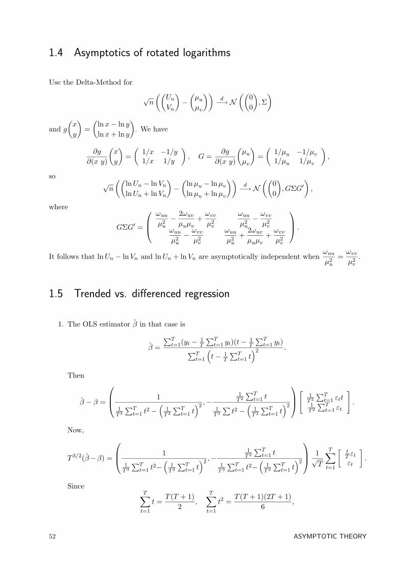
1.4 Asymptotics of rotated logarithms
Let the positive random vector (Un, Vn)′
be such that
√n
((UnVn
)−(µuµv
))d→ N
((00
),
(ωuu ωuvωuv ωvv
))as n→∞. Find the joint asymptotic distribution of(
lnUn − lnVnlnUn + lnVn
).
What is the condition under which lnUn− lnVn and lnUn + lnVn are asymptotically independent?
1.5 Trended vs. differenced regression
Consider a linear model with a linearly trending regressor:
yt = α+ βt+ εt,
where the sequence εt is independently and identically distributed according to some distributionD with mean zero and variance σ2. The object of interest is β.
1. Write out the OLS estimator β of β in deviations form. Find the asymptotic distribution ofβ.
2. An investigator suggests getting rid of the trending regressor by taking differences to obtain
yt − yt−1 = β + εt − εt−1
and estimating β by OLS. Write out the OLS estimator β of β and find its asymptoticdistribution.
3. Compare the estimators β and β in terms of asymptotic efficiency.
12 ASYMPTOTIC THEORY
1.6 Second-order Delta-Method
Let Sn = 1n
∑ni=1Xi, where Xi, i = 1, · · · , n, is an IID sample of scalar random variables with
E [Xi] = µ and V [Xi] = 1. It is easy to show that√n(S2
n − µ2) d→ N (0, 4µ2) when µ 6= 0.
(a) Find the asymptotic distribution of S2n when µ = 0, by taking a square of the asymptotic
distribution of Sn.
(b) Find the asymptotic distribution of cos(Sn). Hint: take a higher order Taylor expansionapplied to cos(Sn).
(c) Using the technique of part (b), formulate and prove an analog of the Delta-Method for thecase when the function is scalar-valued, has zero first derivative and nonzero second derivative,when the derivatives are evaluated at the probability limit. For simplicity, let all the randomvariables be scalars.
1.7 Brief and exhaustive
Give brief but exhaustive answers to the following short questions.
1. Suppose that xt is generated by xt = ρxt−1 + et, where et = εt + θεt−1 and εt is white noise.Is the OLS estimator of ρ consistent?
2. The process for the scalar random variable xt is covariance stationary with the followingautocovariances: 3 at lag 0; 2 at lag 1; 1 at lag 2; and zero for all higher lags. Let T denotethe sample size. What is the long-run variance of xt, i.e. lim
T→∞V
(1√T
∑Tt=1 xt
)?
3. Often one needs to estimate the long-run variance Vze of the stationary sequence ztet thatsatisfies the restriction E[et|zt] = 0. Derive a compact expression for Vze in the case whenet and zt follow independent scalar AR(1) processes. For this example, propose a way toconsistently estimate Vze and show your estimator’s consistency.
1.8 Asymptotics of averages of AR(1) and MA(1)
Let xt be a martingale difference sequence relative to its own past, and let all conditions for theCLT be satisfied:
√TxT = 1√
T
∑Tt=1 xt
d→ N (0, σ2). Let now yt = ρyt−1 + xt and zt = xt + θxt−1,
where |ρ| < 1 and |θ| < 1. Consider time averages yT = 1T
∑Tt=1 yt and zT = 1
T
∑Tt=1 zt.
1. Are yt and zt martingale difference sequences relative to their own past?
2. Find the asymptotic distributions of yT and zT .
3. How would you estimate the asymptotic variances of yT and zT ?
SECOND-ORDER DELTA-METHOD 13
4. Repeat what you did in parts 1–3 when xt is a k×1 vector, and we have√TxT = 1√
T
∑Tt=1 xt
d→N (0,Σ), yt = Pyt−1 + xt, zt = xt + Θxt−1, and P and Θ are k× k matrices with eigenvaluesinside the unit circle.
14 ASYMPTOTIC THEORY
2. BOOTSTRAP
2.1 Brief and exhaustive
Give brief but exhaustive answers to the following short questions.
1. Comment on: ”The only difference between Monte-Carlo and the bootstrap is possibility andimpossibility, respectively, of sampling from the true population.”
2. Comment on: ”When one does bootstrap, there is no reason to raise B too high: there is alevel when increasing B does not give any increase in precision”.
3. Comment on: ”The bootstrap estimator of the parameter of interest is preferable to theasymptotic one, since its rate of convergence to the true parameter is often larger”.
4. Suppose that one got in an application θ = 1.2 and s(θ) = .2. By the nonparametric bootstrapprocedure, the 2.5% and 97.5% bootstrap critical values for the bootstrap distribution of θturned out to be .75 and 1.3. Find: (a) 95% Efron percentile interval for θ, (b) 95% Hallpercentile interval for θ, (c) 95% percentile-t interval for θ.
2.2 Bootstrapping t-ratio
Consider the following bootstrap procedure. Using the nonparametric bootstrap, generate pseu-
dosamples and calculateθ∗b − θs(θ)
at each bootstrap repetition. Find the quantiles q∗α/2 and q∗1−α/2
from this bootstrap distribution, and construct
CI = [θ − s(θ)q∗1−α/2, θ − s(θ)q∗α/2].
Show that CI is exactly the same as Hall’s percentile interval, and not the t-percentile interval.
2.3 Bootstrap correcting mean and its square
Consider a random variable x with mean µ. A random sample xini=1 is available. One estimatesµ by xn and µ2 by x2
n. Find out what the bootstrap bias corrected estimators of µ and µ2 are.
2.4 Bootstrapping conditional mean
Take the linear regressionyi = x′iβ + ei,
BOOTSTRAP 15
with E [ei|xi] = 0. For a particular value of x, the object of interest is the conditional meang(x) = E [yi|x] . Describe how you would use the percentile-t bootstrap to construct a confidenceinterval for g(x).
2.5 Bootstrap adjustment for endogeneity?
Let the model beyi = x′iβ + ei,
but E [eixi] 6= 0, i.e. the regressors are endogenous. Then the OLS estimator β is biased forthe parameter β. We know that the bootstrap is a good way to estimate bias, so the idea is toestimate the bias of β and construct a bias-adjusted estimate of β. Explain whether or not thenon-parametric bootstrap can be used to implement this idea.
16 BOOTSTRAP
3. REGRESSION IN GENERAL
3.1 Property of conditional distribution
Consider a random pair (Y,X). Prove that the correlation coefficient
ρ(Y, f(X)),
where f is any measurable function, is maximized in absolute value when f(X) is linear in E [Y |X] .
3.2 Unobservables among regressors
Consider the following situation. The vector (y, x, z, w) is a random quadruple. It is known that
E [y|x, z, w] = α+ βx+ γz.
It is also known that C [x, z] = 0 and that C [w, z] > 0. The parameters α, β and γ are not known.A random sample of observations on (y, x, w) is available; z is not observable.
In this setting, a researcher weighs two options for estimating β. One is a linear least squaresfit of y on x. The other is a linear least squares fit of y on (x,w). Compare these options.
3.3 Consistency of OLS in presence of lagged dependent variable and
serially correlated errors
1Let yt+∞t=−∞ be a strictly stationary and ergodic stochastic process with zero mean and finitevariance.
(i) Define
β =C [yt, yt−1]V [yt]
, ut = yt − βyt−1,
so that we can writeyt = βyt−1 + ut.
Show that the error ut satisfies E [ut] = 0 and C [ut, yt−1] = 0.
(ii) Show that the OLS estimator β from the regression of yt on yt−1 is consistent for β.
(iii) Show that, without further assumptions, ut is serially correlated. Construct an example withserially correlated ut.
1This problem closely follows J.M. Wooldridge (1998) Consistency of OLS in the Presence of Lagged DependentVariable and Serially Correlated Errors. Econometric Theory 14, Problem 98.2.1.
REGRESSION IN GENERAL 17
(iv) A 1994 paper in the Journal of Econometrics leads with the statement: ”It is well known thatin linear regression models with lagged dependent variables, ordinary least squares (OLS)estimators are inconsistent if the errors are autocorrelated”. This statement, or a slightvariation on it, appears in virtually all econometrics textbooks. Reconcile this statementwith your findings from parts (ii) and (iii).
3.4 Incomplete regression
Consider the linear regression
yi = x′i βk1×1
+ ei, E [ei|xi] = 0, E
[e2i |xi
]= σ2.
Suppose that some component of the error ei is observable, so that
ei = z′i γk2×1
+ ηi,
where zi is a vector of observables such that E [ηi|zi] = 0 and E [xiz′i] 6= 0. The researcher wants toestimate β and γ and considers two alternatives:
1. Run the regression of yi on xi and zi to find the OLS estimates β and γ of β and γ.
2. Run the regression of yi on xi to get the OLS estimate β of β, compute the OLS residualsei = yi − x′iβ and run the regression of ei on zi to retrieve the OLS estimate γ of γ.
Which of the two methods would you recommend from the point of view of consistency ofβ and γ? For the method(s) that yield(s) consistent estimates, find the limiting distribution of√n (γ − γ) .
3.5 Brief and exhaustive
Give brief but exhaustive answers to the following short questions.
1. Comment on: ”Treating regressors x in a linear mean regression y = x′β + e as randomvariables rather than fixed numbers simplifies further analysis, since then the observations(xi, yi) may be treated as IID across i”.
2. A labor economist argues: ”It is more plausible to think of my regressors as random ratherthan fixed. Look at education, for example. A person chooses her level of education, thus itis random. Age may be misreported, so it is random too. Even gender is random, becauseone can get a sex change operation done.” Comment on this pearl.
3. Let (x, y, z) be a random triple. For a given real constant γ a researcher wants to estimateE [y|E [x|z] = γ]. The researcher knows that E [x|z] and E [y|z] are strictly increasing andcontinuous functions of z, and is given consistent estimates of these functions. Show how theresearcher can use them to obtain a consistent estimate of the quantity of interest.
18 REGRESSION IN GENERAL

4. Comment on: ”When one suspects heteroskedasticity, one should use White’s formula
Q−1xxQxxe2Q
−1xx
instead of conventional σ2Q−1xx , since under heteroskedasticity the latter does not make sense,
because σ2 is different for each observation”.
BRIEF AND EXHAUSTIVE 19

20 REGRESSION IN GENERAL
4. OLS AND GLS ESTIMATORS
4.1 Brief and exhaustive
Give brief but exhaustive answers to the following short questions.
1. Consider a linear mean regression yi = x′iβ + ei, E [ei|xi] = 0, where xi, instead of being IIDacross i, depends on i through an unknown function ϕ as xi = ϕ(i) + ui, where ui are IIDindependent of ei. Show that the OLS estimator of β is still unbiased.
2. Consider a model y = (α+βx)e, where y and x are scalar observables, e is unobservable. LetE [e|x] = 1 and V [e|x] = 1. How would you estimate (α, β) by OLS? What standard errors(conventional or White’s) would you construct?
4.2 Estimation of linear combination
Suppose one has an IID random sample of n observations from the linear regression model
yi = α+ βxi + γzi + ei,
where ei has mean zero and variance σ2 and is independent of (xi, zi) .
1. What is the conditional variance of the best linear conditionally (on the xi and zi observations)unbiased estimator θ of
θ = α+ βcx + γcz,
where cx and cz are some given constants?
2. Obtain the limiting distribution of √n(θ − θ
).
Write your answer as a function of the means, variances and correlations of xi, zi and ei andof the constants α, β, γ, cx, cz, assuming that all moments are finite.
3. For what value of the correlation coefficient between xi and zi is the asymptotic varianceminimized for given variances of ei and xi?
4. Discuss the relationship of the result of part 3 with the problem of multicollinearity.
4.3 Long and short regressions
Take the true model Y = X1β1 + X2β2 + e, E [e|X1, X2] = 0. Suppose that β1 is estimated onlyby regressing Y on X1 only. Find the probability limit of this estimator. What are the conditionswhen it is consistent for β1?
OLS AND GLS ESTIMATORS 21
4.4 Ridge regression
In the standard linear mean regression model, one estimates k × 1 parameter β by
β =(X ′X + λIk
)−1X ′Y,
where λ > 0 is a fixed scalar, Ik is a k × k identity matrix, X is n× k and Y is n× 1 matrices ofdata.
1. Find E[β|X
]. Is β conditionally unbiased? Is it unbiased?
2. Find plimn→∞
β. Is β consistent?
3. Find the asymptotic distribution of β.
4. From your viewpoint, why may one want to use β instead of the OLS estimator β? Giveconditions under which β is preferable to β according to your criterion, and vice versa.
4.5 Exponential heteroskedasticity
Let y be scalar and x be k× 1 vector random variables. Observations (yi, xi) are drawn at randomfrom the population of (y, x). You are told that E [y|x] = x′β and that V [y|x] = exp(x′β+α), with(β, α) unknown. You are asked to estimate β.
1. Propose an estimation method that is asymptotically equivalent to GLS that would be com-putable were V [y|x] fully known.
2. In what sense is the feasible GLS estimator of Part 1 efficient? In which sense is it inefficient?
4.6 OLS and GLS are identical
Let Y = X(β+ v) +u, where X is n× k, Y and u are n× 1, and β and v are k× 1. The parameterof interest is β. The properties of (Y,X, u, v) are: E [u|X] = E [v|X] = 0, E [uu′|X] = σ2In,E [vv′|X] = Γ, E [uv′|X] = 0. Y and X are observable, while u and v are not.
1. What are E [Y |X] and V [Y |X]? Denote the latter by Σ. Is the environment homo- orheteroskedastic?
2. Write out the OLS and GLS estimators β and β of β. Prove that in this model they areidentical. Hint: First prove that X ′e = 0, where e is the n× 1 vector of OLS residuals. Nextprove that X ′Σ−1e = 0. Then conclude. Alternatively, use formulae for the inverse of a sumof two matrices. The first method is preferable, being more ”econometric”.
3. Discuss benefits of using both estimators in this model.
22 OLS AND GLS ESTIMATORS
4.7 OLS and GLS are equivalent
Let us have a regression written in a matrix form: Y = Xβ+u, where X is n×k, Y and u are n×1,and β is k×1. The parameter of interest is β. The properties of u are: E [u|X] = 0, E [uu′|X] = Σ.Let it be also known that ΣX = XΘ for some k × k nonsingular matrix Θ.
1. Prove that in this model the OLS and GLS estimators β and β of β have the same finitesample conditional variance.
2. Apply this result to the following regression on a constant:
yi = α+ ui,
where the disturbances are equicorrelated, that is, E [ui] = 0, V [ui] = σ2 and C [ui, uj ] = ρσ2
for i 6= j.
4.8 Equicorrelated observations
Suppose xi = θ + ui, where E [ui] = 0 and
E [uiuj ] =
1 if i = j
γ if i 6= j
with i, j = 1, · · · , n. Is xn = 1n (x1 + · · ·+ xn) the best linear unbiased estimator of θ? Investigate
xn for consistency.
OLS AND GLS ARE EQUIVALENT 23

24 OLS AND GLS ESTIMATORS
5. IV AND 2SLS ESTIMATORS
5.1 Instrumental variables in ARMA models
1. Consider an AR(1) model xt = ρxt−1 + et with E [et|It−1] = 0, E[e2t |It−1
]= σ2, and |ρ| < 1.
We can look at this as an instrumental variables regression that implies, among others, instru-ments xt−1, xt−2, · · · . Find the asymptotic variance of the instrumental variables estimatorthat uses instrument xt−j , where j = 1, 2, · · · . What does your result suggest on what theoptimal instrument must be?
2. Consider an ARMA(1, 1) model yt = αyt−1 +et−θet−1 with |α| < 1, |θ| < 1 and E [et|It−1] =0. Suppose you want to estimate α by just-identifying IV. What instrument would you useand why?
5.2 Inappropriate 2SLS
Consider the modelyi = αz2
i + ui, zi = πxi + vi,
where (xi, ui, vi) are IID, E [ui|xi] = E [vi|xi] = 0 and V[(uivi
)|xi]
= Σ, with Σ unknown.
1. Show that α, π and Σ are identified. Suggest analog estimators for these parameters.
2. Consider the following two stage estimation method. In the first stage, regress zi on xi anddefine zi = πxi, where π is the OLS estimator. In the second stage, regress yi in z2
i to obtainthe least squares estimate of α. Show that the resulting estimator of α is inconsistent.
3. Suggest a method in the spirit of 2SLS for estimating α consistently.
5.3 Inconsistency under alternative
Suppose thaty = α+ βx+ u,
where u is distributed N (0, σ2) independently of x. The variable x is unobserved. Instead weobserve z = x+ v, where v is distributed N (0, η2) independently of x and u. Given a sample of sizen, it is proposed to run the linear regression of y on z and use a conventional t-test to test the nullhypothesis β = 0. Critically evaluate this proposal.
IV AND 2SLS ESTIMATORS 25
5.4 Trade and growth
In the paper ”Does Trade Cause Growth?” (American Economic Review, June 1999), JeffreyFrankel and David Romer study the effect of trade on income. Their simple specification is
log Yi = α+ βTi + γWi + εi, (5.1)
where Yi is per capita income, Ti is international trade, Wi is within-country trade, and εi reflectsother influences on income. Since the latter is likely to be correlated with the trade variables,Frankel and Romer decide to use instrumental variables to estimate the coefficients in (5.1). Asinstruments, they use a country’s proximity to other countries Pi and its size Si, so that
Ti = ψ + φPi + δi (5.2)
andWi = η + λSi + νi, (5.3)
where δi and νi are the best linear prediction errors.
1. As the key identifying assumption, Frankel and Romer use the fact that countries’ geographi-cal characteristics Pi and Si are uncorrelated with the error term in (5.1). Provide an economicrationale for this assumption and a detailed explanation how to estimate (5.1) when one hasdata on Y, T, W, P and S for a list of countries.
2. Unfortunately, data on within-country trade are not available. Determine if it is possible toestimate any of the coefficients in (5.1) without further assumptions. If it is, provide all thedetails on how to do it.
3. In order to be able to estimate key coefficients in (5.1), Frankel and Romer add anotheridentifying assumption that Pi is uncorrelated with the error term in (5.3). Provide a detailedexplanation how to estimate (5.1) when one has data on Y, T, P and S for a list of countries.
4. Frankel and Romer estimated an equation similar to (5.1) by OLS and IV and found outthat the IV estimates are greater than the OLS estimates. One explanation may be that thediscrepancy is due to a sampling error. Provide another, more econometric, explanation whythere is a discrepancy and what the reason is that the IV estimates are larger.
26 IV AND 2SLS ESTIMATORS
6. EXTREMUM ESTIMATORS
6.1 Extremum estimators
Consider the following class of estimators called Extremum Estimators. Let the true parameter βbe the unique solution of the following optimization problem:
β =arg maxb∈B
E [f(z, b)] , (6.1)
where z ∈ Rl is a random vector on which the data are available, b ∈ Rk is a parameter, f is aknown function, B is a parameter space. The latter is assumed to be compact, so that there are noproblems with existence of the optimizer. The data zi, i = 1, ..., n, are IID.
1. Construct the extremum estimator β of β by using the analogy principle applied to (6.1).Assuming that consistency holds, derive the asymptotic distribution of β. Explicitly state allassumptions that you made to derive it.
2. Verify that your answer to part 1 reconciles with the results we obtained in class during thelast module for the NLLS and WNLLS estimators, by appropriately choosing the form offunction f .
6.2 Regression on constant
Apply the results of the previous problem to the following model:
yi = β + ei, i = 1, · · · , n,
where all variables are scalars. Assume that ei are IID with E[ei] = 0, E[e2i ] = β2, E[e3
i ] = 0 andE[e4
i ] = κ. Consider the following three estimators of β:
β1 =1n
n∑i=1
yi,
β2 =arg minb
log b2 +
1nb2
n∑i=1
(yi − b)2
,
β3 =12
arg minb
n∑i=1
(yib− 1)2.
Derive the asymptotic distributions of these three estimators. Which of them would you prefer moston the asymptotic basis? Bonus question: what was the idea behind each of the three estimators?
EXTREMUM ESTIMATORS 27
6.3 Quadratic regression
Consider a nonlinear regression model
yi = (β0 + xi)2 + ui,
where we assume:
(A) Parameter space is B =[−1
2 ,+12
].
(B) ui are IID with E [ui] = 0, V [ui] = σ20.
(C) xi are IID with uniform distribution over [1, 2], distributed independently of ui. Inparticular, this implies E
[x−1i
]= ln 2 and E [xri ] = 1
1+r (2r+1 − 1) for integer r 6= −1.
Define two estimators of β0:
1. β minimizes Sn(β) =∑n
i=1
[yi − (β + xi)
2]2
over B.
2. β minimizes Wn(β) =∑n
i=1
yi
(β + xi)2 + ln (β + xi)
2
over B.
For the case β0 = 0, obtain asymptotic distributions of β and β. Which one of the two do youprefer on the asymptotic basis?
28 EXTREMUM ESTIMATORS
7. MAXIMUM LIKELIHOOD ESTIMATION
7.1 MLE for three distributions
1. A random variable X is said to have a Pareto distribution with parameter λ, denoted X ∼Pareto(λ), if it is continuously distributed with density
fX(x|λ) =λx−(λ+1), if x > 1,0, otherwise.
A random sample x1, · · · , xn from the Pareto(λ) population is available.
(i) Derive the ML estimator λ of λ, prove its consistency and find its asymptotic distribution.
(ii) Derive the Wald, Likelihood Ratio and Lagrange Multiplier test statistics for testing thenull hypothesis H0 : λ = λ0 against the alternative hypothesis Ha : λ 6= λ0. Do any ofthese statistics coincide?
2. Let x1, · · · , xn be a random sample from N (µ, µ2). Derive the ML estimator µ of µ and proveits consistency.
3. Let x1, · · · , xn be a random sample from a population of x distributed uniformly on [0, θ].Construct an asymptotic confidence interval for θ with significance level 5% by employing amaximum likelihood approach.
7.2 Comparison of ML tests
1Berndt and Savin in 1977 showed that W ≥ LR ≥ LM for the case of a multivariate regressionmodel with normal disturbances. Ullah and Zinde-Walsh in 1984 showed that this inequality isnot robust to non-normality of the disturbances. In the spirit of the latter article, this problemconsiders simple examples from non-normal distributions and illustrates how this conflict amongcriteria is affected.
1. Consider a random sample x1, · · · , xn from a Poisson distribution with parameter λ. Showthat testing λ = 3 versus λ 6= 3 yields W ≥ LM for x ≤ 3 and W ≤ LM for x ≥ 3.
2. Consider a random sample x1, · · · , xn from an exponential distribution with parameter θ.Show that testing θ = 3 versus θ 6= 3 yields W ≥ LM for 0 < x ≤ 3 and W ≤ LM for x ≥ 3.
3. Consider a random sample x1, · · · , xn from a Bernoulli distribution with parameter θ. Showthat for testing θ = 1
2 versus θ 6= 12 , we always getW ≥ LM. Show also that for testing θ = 2
3versus θ 6= 2
3 , we get W ≤ LM for 13 ≤ x ≤
23 and W ≥ LM for 0 < x ≤ 1
3 or 23 ≤ x ≤ 1.
1This problem closely follows Badi H. Baltagi (2000) Conflict Among Criteria for Testing Hypotheses: Examplesfrom Non-Normal Distributions. Econometric Theory 16, Problem 00.2.4.
MAXIMUM LIKELIHOOD ESTIMATION 29
7.3 Individual effects
Suppose (xi, yi)ni=1 is a serially independent sample from a sequence of jointly normal distributionswith E [xi] = E [yi] = µi, V [xi] = V [yi] = σ2, and C [xi, yi] = 0 (i.e., xi and yi are independentwith common but varying means and a constant common variance). All parameters are unknown.Derive the maximum likelihood estimate of σ2 and show that it is inconsistent. Explain why. Findan estimator of σ2 which would be consistent.
7.4 Does the link matter?
2Consider a binary random variable y and a scalar random variable x such that
P y = 1|x = F (α+ βx) ,
where the link F (·) is a continuous distribution function. Show that when x assumes only twodifferent values, the value of the log-likelihood function evaluated at the maximum likelihood esti-mates of α and β is independent of the form of the link function. What are the maximum likelihoodestimates of α and β?
7.5 Nuisance parameter in density
Let zi ≡ (yi, x′i)′ have a joint density of the form
f(Z|θ0) = fc(Y |X, γ0, δ0)fm(X|δ0),
where θ0 ≡ (γ0, δ0), both γ0 and δ0 are scalar parameters, and fc and fm denote the conditionaland marginal distributions, respectively. Let θc ≡ (γc, δc) be the conditional ML estimators of γ0
and δ0, and δm be the marginal ML estimator of δ0. Now define
γ ≡ arg maxγ
∑i
ln fc(yi|xi, γ, δm),
a two-step estimator of subparameter γ0 which uses marginal ML to obtain a preliminary estimatorof the ”nuisance parameter” δ0. Find the asymptotic distribution of γ. How does it compare tothat for γc? You may assume all the needed regularity conditions for consistency and asymptoticnormality to hold.
Hint: You need to apply the Taylor’s expansion twice, i.e. for both stages of estimation.
7.6 MLE versus OLS
Consider the model where yi is regressed only on a constant:
yi = α+ ei, i = 1, . . . , n,2This problem closely follows Joao M.C. Santos Silva (1999) Does the link matter? Econometric Theory 15,
Problem 99.5.3.
30 MAXIMUM LIKELIHOOD ESTIMATION
where ei conditioned on xi is distributed as N (0, x2iσ
2); xi’s are drawn from a population of somerandom variable x that is not present in the regression; σ2 is unknown; yi’s and xi’s are observable,ei’s are unobservable; the pairs (yi, xi) are IID.
1. Find the OLS estimator αOLS of α. Is it unbiased? Consistent? Obtain its asymptoticdistribution. Is αOLS the best linear unbiased estimator for α?
2. Find the ML estimator αML of α and derive its asymptotic distribution. Is αML unbiased? IsαML asymptotically more efficient than αOLS? Does your conclusion contradicts your answerto the last question of part 1? Why or why not?
7.7 MLE in heteroskedastic time series regression
Assume that data (yt, xt), t = 1, 2, · · · , T, are stationary and ergodic and generated by
yt = α+ βxt + ut,
where ut|xt ∼ N (0, σ2t ), xt ∼ N (0, v), E[utus|xt, xs] = 0, t 6= s. Explain, without going into deep
math, how to find estimates and their standard errors for all parameters when:
1. The entire σ2t as a function of xt is fully known.
2. The values of σ2t at t = 1, 2, · · · , T are known.
3. It is known that σ2t = (θ + δxt)2, but the parameters θ and δ are unknown.
4. It is known that σ2t = θ + δu2
t−1, but the parameters θ and δ are unknown.
5. It is only known that σ2t is stationary.
7.8 Maximum likelihood and binary variables
Suppose Z and Y are discrete random variables taking values 0 or 1. The distribution of Z and Yis given by
PZ = 1 = α, PY = 1|Z =eγZ
1 + eγZ, Z = 0, 1.
Here α and γ are scalar parameters of interest.
1. Find the ML estimator of (α, γ) (giving an explicit formula whenever possible) and derive itsasymptotic distribution.
2. Suppose we want to test H0 : α = γ using the asymptotic approach. Derive the t test statisticand describe in detail how you would perform the test.
3. Suppose we want to test H0 : α = 12 using the bootstrap approach. Derive the LR (likelihood
ratio) test statistic and describe in detail how you would perform the test.
MLE IN HETEROSKEDASTIC TIME SERIES REGRESSION 31
7.9 Maximum likelihood and binary dependent variable
Suppose y is a discrete random variable taking values 0 or 1 representing some choice of an indi-vidual. The distribution of y given the individual’s characteristic x is
Py = 1|x =eγx
1 + eγx,
where γ is the scalar parameter of interest. The data yi, xi, i = 1, ..., n, are IID. When derivingvarious estimators, try to make the formulas as explicit as possible.
1. Derive the ML estimator of γ and its asymptotic distribution.
2. Find the (nonlinear) regression function by regressing y on x. Derive the NLLS estimator ofγ and its asymptotic distribution.
3. Show that the regression you obtained in Part 2 is heteroskedastic. Setting weights ω(x) equalto the variance of y conditional on x, derive the WNLLS estimator of γ and its asymptoticdistribution.
4. Write out the systems of moment conditions implied by the ML, NLLS and WNLLS problemsof Parts 1–3.
5. Rank the three estimators in terms of asymptotic efficiency. Do any of your findings appearunexpected? Give intuitive explanation for anything unusual.
7.10 Bootstrapping ML tests
1. For the likelihood ratio test of H0 : g(θ) = 0, we use the statistic
LR = 2(
maxq∈Θ
`n(q)− maxq∈Θ,g(q)=0
`n(q)).
Write out the formula (no need to describe the entire algorithm) for the bootstrap pseudo-statistic LR∗.
2. For the Lagrange Multiplier test of H0 : g(θ) = 0, we use the statistic
LM =1n
∑i
s(zi, θ
R
ML
)′J−1
∑i
s(zi, θ
R
ML
).
Write out the formula (no need to describe the entire algorithm) for the bootstrap pseudo-statistic LM∗.
7.11 Trivial parameter space
Consider a parametric model with density f(X|θ0), known up to a parameter θ0, but with Θ = θ1,i.e. the parameter space is reduced to only one element. What is an ML estimator of θ0, and whatare its asymptotic properties?
32 MAXIMUM LIKELIHOOD ESTIMATION
8. GENERALIZED METHOD OF MOMENTS
8.1 GMM and chi-squared
Let z be distributed as χ2(1). Then the moment function
m(z, q) =(
z − qz2 − q2 − 2q
)has mean zero for q = 1. Describe efficient GMM estimation of θ = 1 in details.
8.2 Improved GMM
Consider GMM estimation with the use of the moment function
m(x, y, q) =(x− qy
).
Determine under what conditions the second restriction helps in reducing the asymptotic varianceof the GMM estimator of θ.
8.3 Nonlinear simultaneous equations
Letyi = βxi + ui, xi = γy2
i + vi, i = 1, . . . , n,
where xi’s and yi’s are observable, but ui’s and vi’s are not. The data are IID across i.
1. Suppose we know that E [ui] = E [vi] = 0. When are β and γ identified? Propose analogestimators for these parameters.
2. Let also be known that E [uivi] = 0.
(a) Propose a method to estimate β and γ as efficiently as possible given the above informa-tion. Your estimator should be fully implementable given the data xi, yini=1. What is theasymptotic distribution of your estimator?
(b) Describe in detail how to test H0 : β = γ = 0 using the bootstrap approach and the Waldtest statistic.
(c) Describe in detail how to test H0 : E [ui] = E [vi] = E [uivi] = 0 using the asymptoticapproach.
GENERALIZED METHOD OF MOMENTS 33
8.4 Trinity for GMM
Derive the three classical tests (W, LR, LM) for the composite null
H0 : θ ∈ Θ0 ≡ θ : h(θ) = 0,
where h : Rk → Rq, for the efficient GMM case. The analog for the Likelihood Ratio test will be
called the Distance Difference test. Hint: treat the GMM objective function as the ”normalizedloglikelihood”, and its derivative as the ”sample score”.
8.5 Testing moment conditions
In the linear modelyi = x′iβ + ui
under random sampling and the unconditional moment restriction E [xiui] = 0, suppose you wantedto test the additional moment restriction E
[xiu
3i
]= 0, which might be implied by conditional
symmetry of the error terms ui.A natural way to test for the validity of this extra moment condition would be to efficiently
estimate the parameter vector β both with and without the additional restriction, and then to checkwhether the corresponding estimates differ significantly. Devise such a test and give step-by-stepinstructions for carrying it out.
8.6 Interest rates and future inflation
Frederic Mishkin in early 90’s investigated whether the term structure of current nominal interestrates can give information about future path of inflation. He specified the following econometricmodel:
πmt − πnt = αm,n + βm,n (imt − int ) + ηm,nt , Et [ηm,nt ] = 0, (8.1)
where πkt is k-periods-into-the-future inflation rate, ikt is the current nominal interest rate for k-periods-ahead maturity, and ηm,nt is the prediction error.
1. Show how (8.1) can be obtained from the conventional econometric model that tests thehypothesis of conditional unbiasedness of interest rates as predictors of inflation. What re-striction on the parameters in (8.1) implies that the term structure provides no informationabout future shifts in inflation? Determine the autocorrelation structure of ηm,nt .
2. Describe in detail how you would test the hypothesis that the term structure provides noinformation about future shifts in inflation, by using overidentifying GMM and asymptotictheory. Make sure that you discuss such issues as selection of instruments, construction ofthe optimal weighting matrix, construction of the GMM objective function, estimation ofasymptotic variance, etc.
3. Describe in detail how you would test for overidentifying restrictions that arose from your setof instruments, using the nonoverlapping blocks bootstrap approach.
34 GENERALIZED METHOD OF MOMENTS
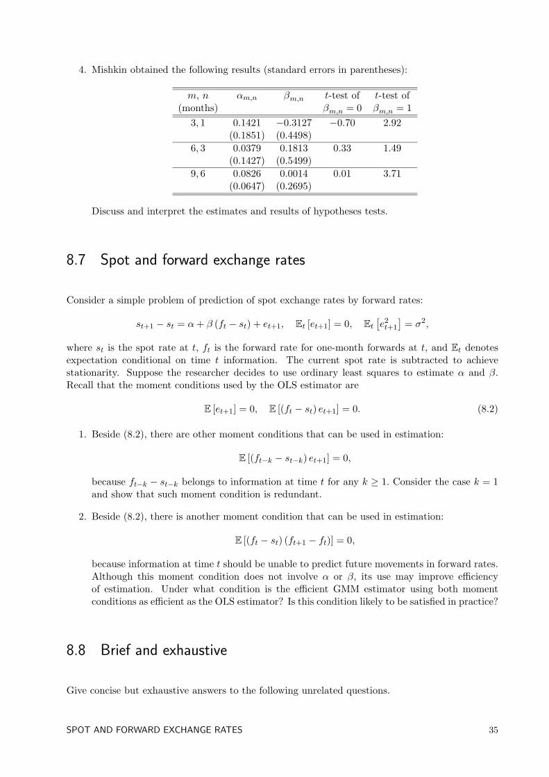
4. Mishkin obtained the following results (standard errors in parentheses):
m, n αm,n βm,n t-test of t-test of(months) βm,n = 0 βm,n = 1
3, 1 0.1421 −0.3127 −0.70 2.92(0.1851) (0.4498)
6, 3 0.0379 0.1813 0.33 1.49(0.1427) (0.5499)
9, 6 0.0826 0.0014 0.01 3.71(0.0647) (0.2695)
Discuss and interpret the estimates and results of hypotheses tests.
8.7 Spot and forward exchange rates
Consider a simple problem of prediction of spot exchange rates by forward rates:
st+1 − st = α+ β (ft − st) + et+1, Et [et+1] = 0, Et
[e2t+1
]= σ2,
where st is the spot rate at t, ft is the forward rate for one-month forwards at t, and Et denotesexpectation conditional on time t information. The current spot rate is subtracted to achievestationarity. Suppose the researcher decides to use ordinary least squares to estimate α and β.Recall that the moment conditions used by the OLS estimator are
E [et+1] = 0, E [(ft − st) et+1] = 0. (8.2)
1. Beside (8.2), there are other moment conditions that can be used in estimation:
E [(ft−k − st−k) et+1] = 0,
because ft−k − st−k belongs to information at time t for any k ≥ 1. Consider the case k = 1and show that such moment condition is redundant.
2. Beside (8.2), there is another moment condition that can be used in estimation:
E [(ft − st) (ft+1 − ft)] = 0,
because information at time t should be unable to predict future movements in forward rates.Although this moment condition does not involve α or β, its use may improve efficiencyof estimation. Under what condition is the efficient GMM estimator using both momentconditions as efficient as the OLS estimator? Is this condition likely to be satisfied in practice?
8.8 Brief and exhaustive
Give concise but exhaustive answers to the following unrelated questions.
SPOT AND FORWARD EXCHANGE RATES 35

1. Let it be known that the scalar random variable w has mean µ and that its fourth central mo-ment equals three times its squared variance (like for a normal random variable). Formulatea system of moment conditions for GMM estimation of µ.
2. Suppose an econometrician estimates parameters of a time series regression by GMM afterhaving chosen an overidentifying vector of instrumental variables. He performs the overiden-tification test and claims: ”A big value of the J-statistic is an evidence against validity of thechosen instruments”. Comment on this claim.
3. We know that one should use recentering when bootstrapping a GMM estimator. We alsoknow that the OLS estimator is one of GMM estimators. However, when we bootstrap theOLS estimator, we calculate β
∗= (X∗′X∗)−1X∗′Y ∗ at each bootstrap repetition, and do not
recenter. Resolve the contradiction.
8.9 Efficiency of MLE in GMM class
We proved that the ML estimator of a parameter is efficient in the class of extremum estimatorsof the same parameter. Prove that it is also efficient in the class of GMM estimators of the sameparameter.
36 GENERALIZED METHOD OF MOMENTS
9. PANEL DATA
9.1 Alternating individual effects
Suppose that the unobservable individual effects in a one-way error component model are differentacross odd and even periods:
yit = µOi + x′itβ + vit for odd t,yit = µEi + x′itβ + vit for even t,
(∗)
where t = 1, 2, · · · , 2T, i = 1, · · ·n. Note that there are 2T observations for each individual. Wewill call (9.1) ”alternating effects” specification. As usual, we assume that vit are IID(0, σ2
v)independent of x’s.
1. There are two ways to arrange the observations: (a) in the usual way, first by individual, thenby time for each individual; (b) first all ”odd” observations in the usual order, then all ”even”observations, so it is as though there are 2N ”individuals” each having T observations. Findout the Q-matrices that wipe out individual effects for both arrangements and explain howthey transform the original equations. For the rest of the problem, choose the Q-matrix toyour liking.
2. Treating individual effects as fixed, describe the Within estimator and its properties. Developan F -test for individual effects, allowing heterogeneity across odd and even periods.
3. Treating individual effects as random and assuming their independence of x’s, v’s and eachother, propose a feasible GLS procedure. Consider two cases: (a) when the variance of”alternating effects” is the same: V
[µOi]
= V
[µEi]
= σ2µ, (b) when the variance of ”alternating
effects” is different: V[µOi]
= σ2O, V
[µEi]
= σ2E , σ2
O 6= σ2E .
9.2 Time invariant regressors
Consider a panel data model
yit = x′itβ + ziγ + µi + vit, i = 1, 2, · · · , n, t = 1, 2, · · · , T,
where n is large and T is small. One wants to estimate β and γ.
1. Explain how to efficiently estimate β and γ under (a) fixed effects, (b) random effects, when-ever it is possible. State clearly all assumptions that you will need.
2. Consider the following proposal to estimate γ. At the first step, estimate the model yit =x′itβ+πi+vit by the least squares dummy variables approach. At the second step, take theseestimates πi and estimate the coefficient of the regression of πi on zi. Investigate the resultingestimator of γ for consistency. Can you suggest a better estimator of γ?
PANEL DATA 37

9.3 First differencing transformation
In a one-way error component model with fixed effects, instead of using individual dummies, onecan alternatively eliminate individual effects by taking the first differencing (FD) transformation.After this procedure one has n(T − 1) equations without individual effects, so the vector β ofstructural parameters can be estimated by OLS. Evaluate this proposal.
38 PANEL DATA
10. NONPARAMETRIC ESTIMATION
10.1 Nonparametric regression with discrete regressor
Let (xi, yi), i = 1, · · · , n be an IID sample from the population of (x, y), where x has a discretedistribution with the support a(1), · · · , a(k), where a(1) < · · · < a(k). Having written the conditionalexpectation E
[y|x = a(j)
]in the form that allows to apply the analogy principle, propose an analog
estimator gj of gj = E
[y|x = a(j)
]and derive its asymptotic distribution.
10.2 Nonparametric density estimation
Suppose we have an IID sample xini=1 and let
F (x) =1n
n∑i=1
I [xi ≤ x]
denote the empirical distribution function if xi, where I(·) is an indicator function. Consider twodensity estimators: one-sided estimator:
f1(x) =F (x+ h)− F (x)
h two-sided estimator:
f2(x) =F (x+ h/2)− F (x− h/2)
hShow that:
(a) F (x) is an unbiased estimator of F (x). Hint: recall that F (x) = Pxi ≤ x = E [I [xi ≤ x]] .
(b) The bias of f1(x) is O (ha) . Find the value of a. Hint: take a second-order Taylor seriesexpansion of F (x+ h) around x.
(c) The bias of f2(x) is O(hb). Find the value of b. Hint: take a second-order Taylor series
expansion of F(x+ h
2
)and F
(x+ h
2
)around x.
Now suppose that we want to estimate the density at the sample mean xn, the sample minimumx(1) and the sample maximum x(n). Given the results in (b) and (c), what can we expect from theestimates at these points?
10.3 First difference transformation and nonparametric regression
This problem illustrates the use of a difference operator in nonparametric estimation with IID data.Suppose that there is a scalar variable z that takes values on a bounded support. For simplicity,
NONPARAMETRIC ESTIMATION 39
let z be deterministic and compose a uniform grid on the unit interval [0, 1]. The other variablesare IID. Assume that for the function g (·) below the following Lipschitz condition is satisfied:
|g(u)− g(v)| ≤ G|u− v|
for some constant G.
1. Consider a nonparametric regression of y on z:
yi = g(zi) + ei, i = 1, · · · , n, (10.1)
where E [ei|zi] = 0. Let the data (zi, yi)ni=1 be ordered so that the z’s are in increasingorder. A first difference transformation results in the following set of equations:
yi − yi−1 = g(zi)− g(zi−1) + ei − ei−1, i = 2, · · · , n. (10.2)
The target is to estimate σ2 ≡ E[e2i
]. Propose its consistent estimator based on the FD-
transformed regression (2). Prove consistency of your estimator.
2. Consider the following partially linear regression of y on x and z:
yi = x′iβ + g(zi) + ei, i = 1, · · · , n, (10.3)
where E [ei|xi, zi] = 0. Let the data (xi, zi, yi)ni=1 be ordered so that the z’s are in increasingorder. The target is to nonparametrically estimate g. Propose its consistent estimator basedon the FD-transformation of (3). [Hint: on the first step, consistently estimate β from theFD-transformed regression.] Prove consistency of your estimator.
40 NONPARAMETRIC ESTIMATION
11. CONDITIONAL MOMENT RESTRICTIONS
11.1 Usefulness of skedastic function
Suppose that for the following linear regression model
yi = x′iβ + ei, E [ei|xi] = 0
the form of a skedastic function is
E
[e2i |xi
]= h(xi, β, π),
where h(·) is a known smooth function, and π is an additional parameter vector. Compare asymp-totic variances of optimal GMM estimators of β when only the first restriction or both restrictionsare employed. Under what conditions does including the second restriction into a set of momentrestrictions reduce asymptotic variance? Try to answer these questions in the general case, thenspecialize to the following cases:
1. the function h(·) does not depend on β;
2. the function h(·) does not depend on β and the distribution of ei conditional on xi is sym-metric.
11.2 Symmetric regression error
Suppose that it is known that the equation
y = αx+ e
is a regression of y on x, i.e. that E [e|x] = 0. All variables are scalars. The random sampleyi, xini=1 is available.
1. The investigator also suspects that y, conditional on x, is distributed symmetrically aroundthe conditional mean. Devise a Hausman specification test for this symmetry. Be specificand give all details at all stages when constructing the test.
2. Suppose that even though the Hausman test rejects symmetry, the investigator uses theassumption that e|x ∼ N (0, σ2). Derive the asymptotic properties of the QML estimator ofα.
11.3 Optimal instrument in AR-ARCH model
Consider an AR(1) − ARCH(1) model: xt = ρxt−1 + εt where the distribution of εt conditionalon It−1 is symmetric around 0 with E
[ε2t |It−1
]= (1 − α) + αε2
t−1, where 0 < ρ, α < 1 andIt = xt, xt−1, · · · .
CONDITIONAL MOMENT RESTRICTIONS 41
1. Let the space of admissible instruments for estimation of the AR(1) part be
Zt =
∞∑i=1
φixt−i, s.t.∞∑i=1
φ2i <∞
.
Using the optimality condition, find the optimal instrument as a function of the model pa-rameters ρ and α. Outline how to construct its feasible version.
2. Use your intuition to speculate on relative efficiency of the optimal instrument you found inPart 1 versus the optimal instrument based on the conditional moment restriction E [εt|It−1] =0.
11.4 Modified Poisson regression and PML estimators
1Let the observable random variable y be distributed, conditionally on observable x and unobserv-able ε as Poisson with the parameter λ(x) = exp(x′β+ε), where E[exp ε|x] = 1 and V[exp ε|x] = σ2.Suppose that vector x is distributed as multivariate standard normal.
1. Find the regression and skedastic functions, where the conditional information involves onlyx.
2. Find the asymptotic variances of the Nonlinear Least Squares (NLLS) and Weighted NonlinearLeast Squares (WNLLS) estimators of β.
3. Find the asymptotic variances of the Pseudo-Maximum Likelihood (PML) estimators of βbased on
(a) the normal distribution;
(b) the Poisson distribution;
(c) the Gamma distribution.
4. Rank the five estimators in terms of asymptotic efficiency.
11.5 Optimal instrument and regression on constant
Consider the following model:yi = α+ ei, i = 1, . . . , n,
where unobservable ei conditionally on xi is distributed symmetrically with mean zero and variancex2iσ
2 with unknown σ2. The data (yi, xi) are IID.
1. Construct a pair of conditional moment restrictions from the information about the condi-tional mean and conditional variance. Derive the optimal unconditional moment restrictions,corresponding to (a) the conditional restriction associated with the conditional mean; (b) theconditional restrictions associated with both the conditional mean and conditional variance.
1The idea of this problem is borrowed from Gourieroux, C. and Monfort, A. ”Statistics and Econometric Models”,Cambridge University Press, 1995.
42 CONDITIONAL MOMENT RESTRICTIONS

2. Describe in detail the GMM estimators that correspond to the two optimal sets of uncondi-tional moment restrictions of part 1. Note that in part 1(a) the parameter σ2 is not identified,therefore propose your own estimator of σ2 that differs from the one implied by part 1(b). Allestimators that you construct should be fully feasible. If you use nonparametric estimation,give all the details. Your description should also contain estimation of asymptotic variances.
3. Compare the asymptotic properties of the GMM estimators that you designed.
4. Derive the Pseudo-Maximum Likelihood estimator of α and σ2 of order 2 (PML2) that isbased on the normal distribution. Derive its asymptotic properties. How does this estimatorrelate to the GMM estimators you obtained in part 2?
OPTIMAL INSTRUMENT AND REGRESSION ON CONSTANT 43

44 CONDITIONAL MOMENT RESTRICTIONS
12. EMPIRICAL LIKELIHOOD
12.1 Common mean
Suppose we have the following moment restrictions: E [x] = E [y] = θ.
1. Find the system of equations that yield the maximum empirical likelihood (MEL) estimatorθ of θ, the associated Lagrange multipliers λ and the implied probabilities pi. Derive theasymptotic variances of θ and λ and show how to estimate them.
2. Reduce the number of parameters by eliminating the redundant ones. Then linearize thesystem of equations with respect to the Lagrange multipliers that are left, around theirpopulation counterparts of zero. This will help to find an approximate, but explicit solutionfor θ, λ and pi. Derive that solution and interpret it.
3. Instead of defining the objective function
1n
n∑i=1
log pi
as in the EL approach, let the objective function be
− 1n
n∑i=1
pi log pi.
This gives rise to the exponential tilting (ET) estimator of θ. Find the system of equationsthat yields the ET estimator of θ, the associated Lagrange multipliers λ and the impliedprobabilities pi. Derive the asymptotic variances of θ and λ and show how to estimate them.
12.2 Kullback–Leibler Information Criterion
The Kullback–Leibler Information Criterion (KLIC) measures the distance between distributions,say g(z) and h(z):
KLIC(g : h) = Eg
[log
g(z)h(z)
],
where Eg [·] denotes mathematical expectation according to g(z).Suppose we have the following moment condition:
E
[m(zi, θ0
k×1)]
= 0`×1
, ` ≥ k,
and an IID sample z1, · · · , zn with no elements equal to each other. Denote by e the empiricaldistribution function (EDF), i.e. the one that assigns probability 1
n to each sample point. Denoteby π a discrete distribution that assigns probability πi to the sample point zi, i = 1, · · · , n.
EMPIRICAL LIKELIHOOD 45
1. Show that minimization of KLIC(e : π) subject to∑n
i=1 πi = 1 and∑n
i=1 πim(zi, θ) =0 yields the Maximum Empirical Likelihood (MEL) value of θ and corresponding impliedprobabilities.
2. Now we switch the roles of e and π and consider minimization of KLIC(π : e) subject tothe same constraints. What familiar estimator emerges as the solution to this optimizationproblem?
3. Now suppose that we have a priori knowledge about the distribution of the data. So, insteadof using the EDF, we use the distribution p that assigns known probability pi to the samplepoint zi, i = 1, · · · , n (of course,
∑ni=1 pi = 1). Analyze how the solutions to the optimization
problems in parts 1 and 2 change.
4. Now suppose that we have postulated a family of densities f(z, θ) which is compatible withthe moment condition. Interpret the value of θ that minimizes KLIC(e : f).
46 EMPIRICAL LIKELIHOOD

Part II
Solutions
47

1. ASYMPTOTIC THEORY
1.1 Asymptotics of t-ratios
The solution is straightforward, once we determine to what vector to apply LLN and CLT.
(a) When µ = 0, we have: Xp→ 0,
√nX
d→ N (0, σ2), and σ2 p→ σ2, therefore
√nTn =
√nX
σ
d→ 1σN (0, σ2) = N (0, 1)
(b) Consider the vector
Wn ≡(X
σ2
)=
1n
n∑i=1
(Xi
(Xi − µ)2
)−(
0(X − µ)2
).
Due to the LLN, the last term goes in probability to the zero vector, and the first term, andthus the whole Wn, converges in probability to
plimn→∞
Wn =(
µσ2
).
Moreover, since√n(X − µ
) d→ N (0, σ2), we have√n(X − µ
)2 d→ 0.
Next, let Wi ≡(Xi (Xi − µ)2
)′. Then√n
(Wn− plim
n→∞Wn
)d→ N (0, V ), where V ≡ V [Wi].
Let us calculate V . First, V [Xi] = σ2 and V[(Xi − µ)2
]= E
[((Xi − µ)2 − σ2)2
]= τ − σ4.
Second, C[Xi, (Xi − µ)2
]= E
[(Xi − µ)((Xi − µ)2 − σ2)
]= 0. Therefore,
√n
(Wn− plim
n→∞Wn
)d→ N
((00
),
(σ2 00 τ − σ4
))Now use the Delta-Method with function
g
(t1t2
)≡ t1√
t2⇒ g′
(t1t2
)=
1√t2
1
− t12t2
to get
√n
(Tn− plim
n→∞Tn
)d→ N
(0, 1 +
µ2(τ − σ4)4σ6
).
Indeed, the answer reduces to N (0, 1) when µ = 0.
(c) Similarly we solve this part. Consider the vector
Wn ≡(Xσ2
)=
1n
n∑i=1
(Xi
X2i
).
ASYMPTOTIC THEORY 49
Due to the LLN, Wn, converges in probability to
plimn→∞
Wn =(
µµ2 + σ2
).
Next,√n
(Wn− plim
n→∞Wn
)d→ N (0, V ), where V ≡ V [Wi], Wi ≡
(Xi X
2i
)′. Let us calcu-
late V . First, V [Xi] = σ2 and V[X2i
]= E
[(X2
i − µ2 − σ2)2]
= τ + 4µ2σ2 − σ4. Second,C
[Xi, X
2i
]= E
[(Xi − µ)(X2
i − µ2 − σ2)]
= 2µσ2. Therefore,
√n
(Wn− plim
n→∞Wn
)d→ N
((00
),
(σ2 2µσ2
2µσ2 τ + 4µ2σ2 − σ4
))
Now use the Delta-Method with g
(t1t2
)=
t1√t2
to get
√n
(Rn− plim
n→∞Rn
)d→ N
(0,µ2τ − µ2σ4 + 4σ6)
4(µ2 + σ2)3
).
The answer reduces to that of Part (b) iff µ = 0. Under this condition, Tn and Rn areasymptotically equivalent .
1.2 Asymptotics with shrinking regressor
The formulae for the OLS estimators are
β =1n
∑i yixi −
1n2
∑i yi∑
i xi1n
∑i x
2i −
(1n
∑i xi)2 , α = y − βx, σ2 =
1n
∑i
ei2. (1.1)
Let us talk about β first. From (1.1) it follows that
β =1n
∑i(α+ βxi + ui)xi − 1
n2
∑i(α+ βxi + ui)
∑i xi
1n
∑i x
2i − ( 1
n
∑i xi)2
= β +1n
∑i ρiui − 1
n2
∑i ui∑
i ρi
1n
∑i ρ
2i − 1n2 (∑
i ρi)2
= β +
∑i ρiui − ρ(1−ρ1+n)
1−ρ(
1n
∑i ui)
ρ2(1−ρ2(n+1))1−ρ2 − 1
n
(ρ(1−ρ(n+1))
1−ρ
)2
which converges to
β +1− ρ2
ρ2plimn→∞
n∑i=1
ρiui,
if ξ ≡ plim∑
i ρiui exists and is a well-defined random variable. It has E [ξ] = 0, E
[ξ2]
= σ2 ρ2
1−ρ2
and E[ξ3]
= ν ρ3
1−ρ3 . Hence
β − β d→ 1− ρ2
ρ2ξ. (1.2)
Now let us look at α. Again, from (1.1) we see that
α = α+ (β − β) · 1n
∑i
ρi +1n
∑i
uip→ α,
50 ASYMPTOTIC THEORY
where we used (1.2) and the LLN for ui. Next,
√n(α− α) =
1√n
(β − β)ρ(1− ρ1+n)
1− ρ+
1√n
∑i
ui = Un + Vn.
Because of (1.2), Unp→ 0. From the CLT it follows that Vn
d→ N (0, σ2). Together,
√n(α− α) d→ N (0, σ2).
Lastly, let us look at σ2:
σ2 =1n
∑i
e2i =
1n
∑i
((α− α) + (β − β)xi + ui
)2. (1.3)
Using the facts that: (1) (α − α)2 p→ 0, (2) (β − β)2/np→ 0, (3) 1
n
∑i u
2i
p→ σ2, (4) 1n
∑i ui
p→ 0,(5) 1√
n
∑i ρiui
p→ 0, we can derive that
σ2 p→ σ2.
The rest of this solution is optional and is usually not meant when the asymptotics of σ2 isconcerned. Before proceeding to deriving its asymptotic distribution, we would like to mark outthat (β − β)/nδ
p→ 0 and (∑
i ρiui)/nδ
p→ 0 for any δ > 0. Using the same algebra as before wehave
√n(σ2 − σ2) A∼ 1√
n
∑i
(u2i − σ2),
since the other terms converge in probability to zero. Using the CLT, we get
√n(σ2 − σ2) d→ N (0,m4),
where m4 = E
[u4i
]− σ4, provided that it is finite.
1.3 Creeping bug on simplex
Since xk and yk are perfectly correlated, it suffices to consider either one, say, xk. Note that ateach step xk increases by 1
k with probability p, or stays the same. That is, xk = xk−1 + 1kξk, where
ξk is IID Bernoulli(p). This means that xk = 1k
∑ki=1 ξi which by the LLN converges in probability
to E [ξi] = p as k →∞. Therefore, plim(xk, yk) = (p, 1− p). Next, due to the CLT,
√n (xk − plimxk)
d→ N (0, p(1− p)) .
Therefore, the rate of convergence is√n, as usual, and
√n
((xkyk
)− plim
(xkyk
))d→ N
((00
),
(p(1− p) −p(1− p)−p(1− p) p(1− p)
)).
CREEPING BUG ON SIMPLEX 51
1.4 Asymptotics of rotated logarithms
Use the Delta-Method for
√n
((UnVn
)−(µuµv
))d−→ N
((00
),Σ)
and g
(x
y
)=(
lnx− ln ylnx+ ln y
). We have
∂g
∂(x y)
(x
y
)=(
1/x −1/y1/x 1/y
), G =
∂g
∂(x y)
(µuµv
)=(
1/µu −1/µv1/µu 1/µv
),
so√n
((lnUn − lnVnlnUn + lnVn
)−(
lnµu − lnµvlnµu + lnµv
))d−→ N
((00
), GΣG′
),
where
GΣG′ =
ωuuµ2u
− 2ωuvµuµv
+ωvvµ2v
ωuuµ2u
− ωvvµ2v
ωuuµ2u
− ωvvµ2v
ωuuµ2u
+2ωuvµuµv
+ωvvµ2v
.
It follows that lnUn − lnVn and lnUn + lnVn are asymptotically independent whenωuuµ2u
=ωvvµ2v
.
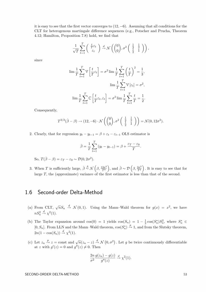
1.5 Trended vs. differenced regression
1. The OLS estimator β in that case is
β =∑T
t=1(yt − 1T
∑Tt=1 yt)(t−
1T
∑Tt=1 yt)∑T
t=1
(t− 1
T
∑Tt=1 t
)2 .
Then
β − β =
11T 3
∑Tt=1 t
2 −(
1T 2
∑Tt=1 t
)2 ,−1T 2
∑Tt=1 t
1T 3
∑t2 −
(1T 2
∑Tt=1 t
)2
[ 1T 3
∑Tt=1 εtt
1T 2
∑Tt=1 εt
].
Now,
T 3/2(β−β) =
11T 3
∑Tt=1 t
2−(
1T 2
∑Tt=1 t
)2 ,−1T 2
∑Tt=1 t
1T 3
∑Tt=1 t
2−(
1T 2
∑Tt=1 t
)2
1√T
T∑t=1
[tT εtεt
].
SinceT∑t=1
t =T (T + 1)
2,
T∑t=1
t2 =T (T + 1)(2T + 1)
6,
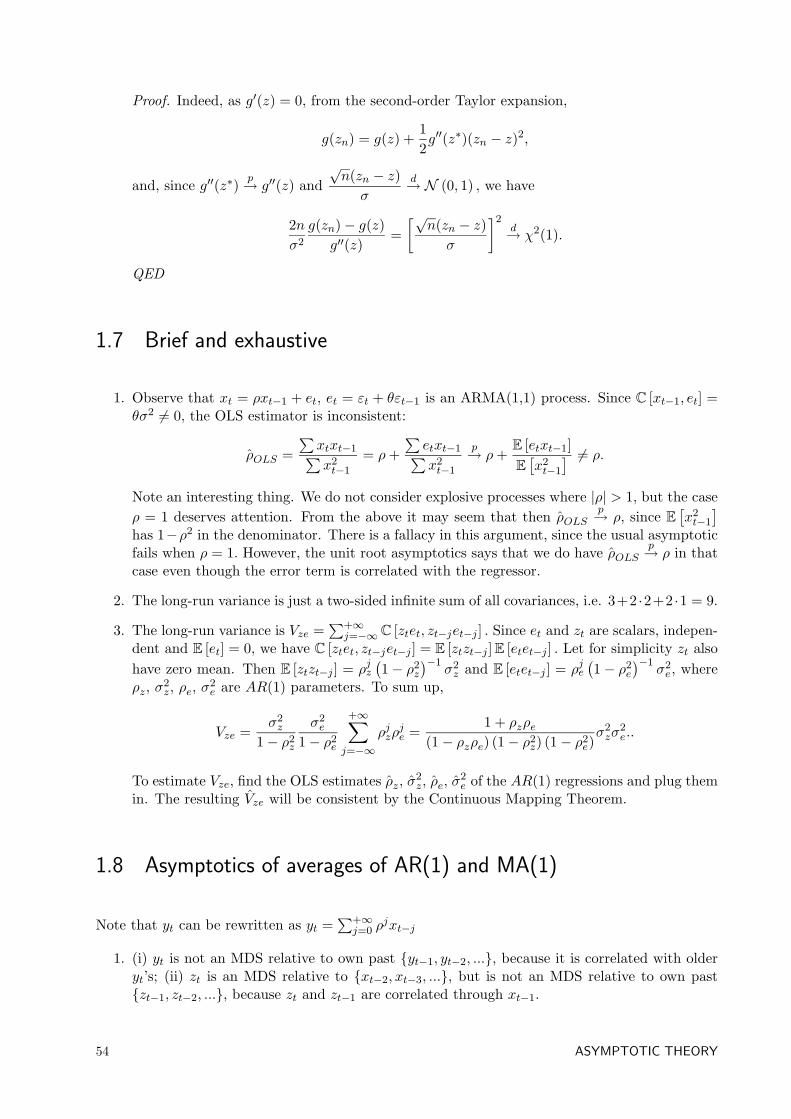
52 ASYMPTOTIC THEORY
it is easy to see that the first vector converges to (12,−6). Assuming that all conditions for theCLT for heterogenous martingale difference sequences (e.g., Potscher and Prucha, Theorem4.12; Hamilton, Proposition 7.8) hold, we find that
1√T
T∑t=1
(tT εtεt
)d→ N
((00
), σ2
(13
12
12 1
)),
since
lim1T
T∑t=1
V
[t
Tεt
]= σ2 lim
1T
T∑t=1
(t
T
)2
=13,
lim1T
T∑t=1
V [εt] = σ2,
lim1T
T∑t=1
C
[t
Tεt, εt
]= σ2 lim
1T
T∑t=1
t
T=
12.
Consequently,
T 3/2(β − β)→ (12,−6) · N((
00
), σ2
(13
12
12 1
))= N (0, 12σ2).
2. Clearly, that for regression yt − yt−1 = β + εt − εt−1 OLS estimator is
β =1T
T∑t=1
(yt − yt−1) = β +εT − ε0
T.
So, T (β − β) = εT − ε0 ∼ D(0, 2σ2).
3. When T is sufficiently large, β A∼ N(β, 12σ2
T 3
), and β ∼ D
(β, 2σ2
T 2
). It is easy to see that for
large T, the (approximate) variance of the first estimator is less than that of the second.
1.6 Second-order Delta-Method
(a) From CLT,√nSn
d→ N (0, 1). Using the Mann–Wald theorem for g(x) = x2, we havenS2
nd→ χ2(1).
(b) The Taylor expansion around cos(0) = 1 yields cos(Sn) = 1 − 12 cos(S∗n)S2
n, where S∗n ∈[0, Sn]. From LLN and the Mann–Wald theorem, cos(S∗n)
p→ 1, and from the Slutsky theorem,2n(1− cos(Sn)) d→ χ2(1).
(c) Let znp→ z = const and
√n(zn − z)
d→ N(0, σ2
). Let g be twice continuously differentiable
at z with g′(z) = 0 and g′′(z) 6= 0. Then
2nσ2
g(zn)− g(z)g′′(z)
d→ χ2(1).
SECOND-ORDER DELTA-METHOD 53
Proof. Indeed, as g′(z) = 0, from the second-order Taylor expansion,
g(zn) = g(z) +12g′′(z∗)(zn − z)2,
and, since g′′(z∗)p→ g′′(z) and
√n(zn − z)
σ
d→ N (0, 1) , we have
2nσ2
g(zn)− g(z)g′′(z)
=[√
n(zn − z)σ
]2d→ χ2(1).
QED
1.7 Brief and exhaustive
1. Observe that xt = ρxt−1 + et, et = εt + θεt−1 is an ARMA(1,1) process. Since C [xt−1, et] =θσ2 6= 0, the OLS estimator is inconsistent:
ρOLS =∑xtxt−1∑x2t−1
= ρ+∑etxt−1∑x2t−1
p→ ρ+E [etxt−1]E
[x2t−1
] 6= ρ.
Note an interesting thing. We do not consider explosive processes where |ρ| > 1, but the caseρ = 1 deserves attention. From the above it may seem that then ρOLS
p→ ρ, since E[x2t−1
]has 1−ρ2 in the denominator. There is a fallacy in this argument, since the usual asymptoticfails when ρ = 1. However, the unit root asymptotics says that we do have ρOLS
p→ ρ in thatcase even though the error term is correlated with the regressor.
2. The long-run variance is just a two-sided infinite sum of all covariances, i.e. 3+2 ·2+2 ·1 = 9.
3. The long-run variance is Vze =∑+∞
j=−∞C [ztet, zt−jet−j ] . Since et and zt are scalars, indepen-dent and E [et] = 0, we have C [ztet, zt−jet−j ] = E [ztzt−j ]E [etet−j ] . Let for simplicity zt alsohave zero mean. Then E [ztzt−j ] = ρjz
(1− ρ2
z
)−1σ2z and E [etet−j ] = ρje
(1− ρ2
e
)−1σ2e, where
ρz, σ2z, ρe, σ
2e are AR(1) parameters. To sum up,
Vze =σ2z
1− ρ2z
σ2e
1− ρ2e
+∞∑j=−∞
ρjzρje =
1 + ρzρe(1− ρzρe) (1− ρ2
z) (1− ρ2e)σ2zσ
2e..
To estimate Vze, find the OLS estimates ρz, σ2z, ρe, σ
2e of the AR(1) regressions and plug them
in. The resulting Vze will be consistent by the Continuous Mapping Theorem.
1.8 Asymptotics of averages of AR(1) and MA(1)
Note that yt can be rewritten as yt =∑+∞
j=0 ρjxt−j
1. (i) yt is not an MDS relative to own past yt−1, yt−2, ..., because it is correlated with olderyt’s; (ii) zt is an MDS relative to xt−2, xt−3, ..., but is not an MDS relative to own pastzt−1, zt−2, ..., because zt and zt−1 are correlated through xt−1.
54 ASYMPTOTIC THEORY
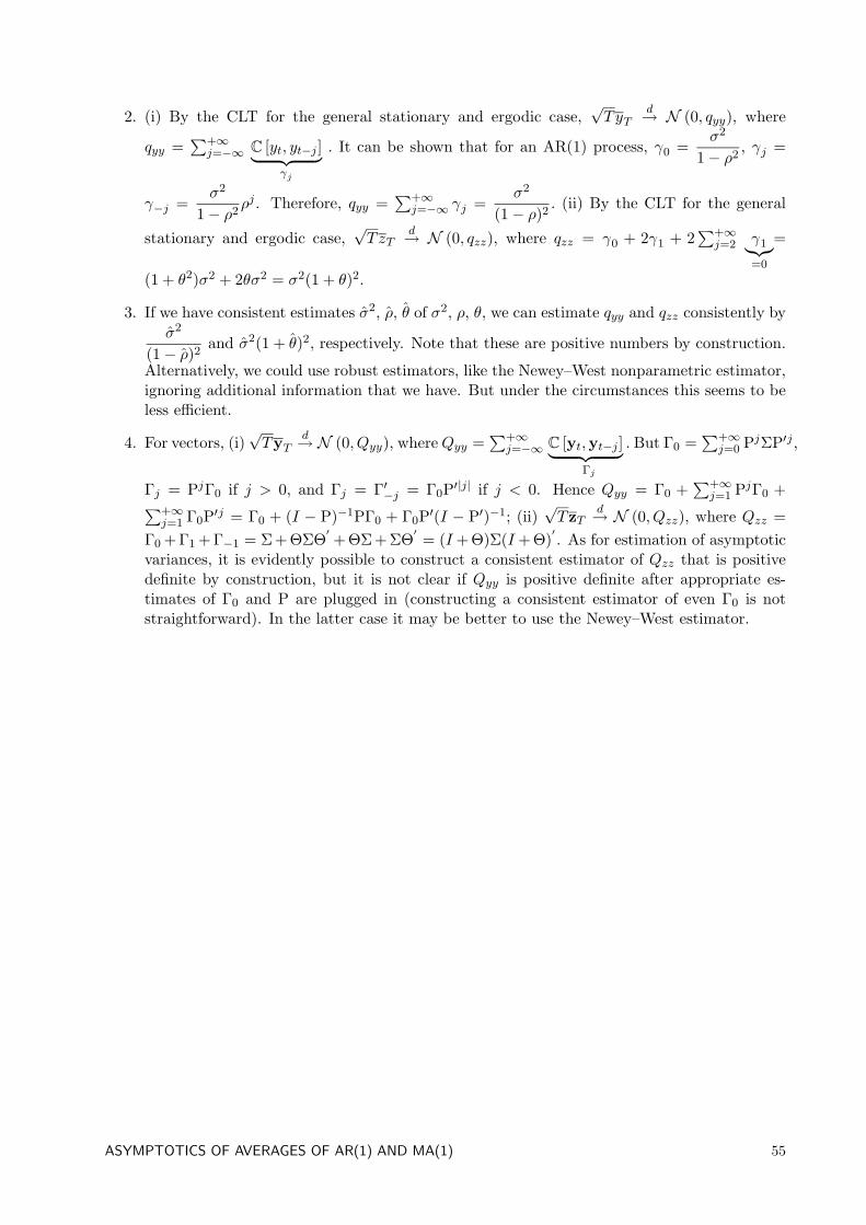
2. (i) By the CLT for the general stationary and ergodic case,√TyT
d→ N (0, qyy), where
qyy =∑+∞
j=−∞ C [yt, yt−j ]︸ ︷︷ ︸γj
. It can be shown that for an AR(1) process, γ0 =σ2
1− ρ2, γj =
γ−j =σ2
1− ρ2ρj . Therefore, qyy =
∑+∞j=−∞ γj =
σ2
(1− ρ)2. (ii) By the CLT for the general
stationary and ergodic case,√TzT
d→ N (0, qzz), where qzz = γ0 + 2γ1 + 2∑+∞
j=2 γ1︸︷︷︸=0
=
(1 + θ2)σ2 + 2θσ2 = σ2(1 + θ)2.
3. If we have consistent estimates σ2, ρ, θ of σ2, ρ, θ, we can estimate qyy and qzz consistently byσ2
(1− ρ)2and σ2(1 + θ)2, respectively. Note that these are positive numbers by construction.
Alternatively, we could use robust estimators, like the Newey–West nonparametric estimator,ignoring additional information that we have. But under the circumstances this seems to beless efficient.
4. For vectors, (i)√TyT
d→ N (0, Qyy), whereQyy =∑+∞
j=−∞ C [yt,yt−j ]︸ ︷︷ ︸ .Γj
But Γ0 =∑+∞
j=0 PjΣP′j ,
Γj = PjΓ0 if j > 0, and Γj = Γ′−j = Γ0P′|j| if j < 0. Hence Qyy = Γ0 +∑+∞
j=1 PjΓ0 +∑+∞j=1 Γ0P′j = Γ0 + (I − P)−1PΓ0 + Γ0P′(I − P′)−1; (ii)
√TzT
d→ N (0, Qzz), where Qzz =Γ0 + Γ1 + Γ−1 = Σ + ΘΣΘ
′+ ΘΣ + ΣΘ
′= (I + Θ)Σ(I + Θ)
′. As for estimation of asymptotic
variances, it is evidently possible to construct a consistent estimator of Qzz that is positivedefinite by construction, but it is not clear if Qyy is positive definite after appropriate es-timates of Γ0 and P are plugged in (constructing a consistent estimator of even Γ0 is notstraightforward). In the latter case it may be better to use the Newey–West estimator.
ASYMPTOTICS OF AVERAGES OF AR(1) AND MA(1) 55

56 ASYMPTOTIC THEORY
2. BOOTSTRAP
2.1 Brief and exhaustive
1. The mentioned difference indeed exists, but it is not the principal one. The two methods havesome common features like computer simulations, sampling, etc., but they serve completelydifferent goals. The bootstrap is an alternative to analytical asymptotic theory for makinginferences, while Monte-Carlo is used for studying small-sample properties of the estimators.
2. After some point raising B does not help since the bootstrap distribution is intrinsicallydiscrete, and raising B cannot smooth things out. Even more than that if we’re interestedin quantiles, and we usually are: the quantile for a discrete distribution is a whole interval,and the uncertainty about which point to choose to be a quantile doesn’t disappear when weraise B.
3. There is no such thing as a ”bootstrap estimator”. Bootstrapping is a method of inference,not of estimation. The same goes for an ”asymptotic estimator”.
4. (a) CE = [q∗n(2.5%), q∗n(97.5%)] = [.75, 1.3]. (b) CH = [θ − qθ∗−θ(97.5%), θ − q
θ∗−θ(2.5%)] =
[2θ − q∗n(97.5%), 2θ − q∗n(2.5%)] = [1.1, 1.65].(c) We cannot compute this from the given information, since we need the quantiles of thet-statistic, which are unavailable.
2.2 Bootstrapping t-ratio
The Hall percentile interval is CIH = [θ − q∗1−α/2, θ − q∗α/2], where q∗α is the bootstrap α-quantile
of θ∗ − θ, i.e. α = Pθ∗ − θ ≤ q∗α. But then
q∗α
s(θ)is the α-quantile of
θ∗ − θs(θ)
= T ∗n , since
P
θ∗ − θs(θ)
≤ q∗α
s(θ)
= α. But by construction, the α-quantile of T ∗n is q∗α, hence q∗α = s(θ)q∗α.
Substituting this into CIH , we get the CI as in the problem.
2.3 Bootstrap correcting mean and its square
The bootstrap version x∗n of xn has mean xn with respect to the EDF: E∗ [x∗n] = xn. Thus thebootstrap version of the bias (which is itself zero) is Bias∗(xn) = E
∗ [x∗n] − xn = 0. Therefore, thebootstrap bias corrected estimator of µ is xn − Bias∗(xn) = xn. Now consider the bias of x2
n:
Bias(x2n) = E
[x2n
]− µ2 = V
[x2n
]=
1nV [x] .
BOOTSTRAP 57
Thus the bootstrap version of the bias is the sample analog of this quantity:
Bias∗(x2n) =
1nV∗ [x] =
1n
(1n
∑x2i − x2
n
). Therefore, the bootstrap bias corrected estimator of µ2 is
x2n − Bias∗(x2
n) =n+ 1n
x2n −
1n2
∑x2i .
2.4 Bootstrapping conditional mean
We are interested in g(x) = E [x′β + e|x] = x′β, and as the point estimate we take g(x) = x′β,where β is the OLS estimator for β. To pivotize g(x), we observe that
x′(β − β) d→ N (0, x(E
[xix′i
])−1E
[e2ixix
′i
] (E
[xix′i
])−1x′),
so the appropriate statistic to bootstrap is
tg =x′(β − β)s (g(x))
,
where s (g(x)) =√x (∑xix′i)
−1 (∑ e2ixix
′i
)(∑xix′i)
−1 x′. The bootstrap version is
t∗g =x′(β
∗ − β)s (g∗(x))
,
where s (g∗(x)) =√x (∑x∗ix
∗′i )−1 (∑ e∗2i x
∗ix∗′i
)(∑x∗ix
∗′i )−1 x′. The rest is standard, and the con-
fidence interval isCIt =
[x′β − q∗1−α
2s (g(x)) ;x′β − q∗α
2s (g(x))
],
where q∗α2
and q∗1−α2
are appropriate bootstrap quantiles for t∗g.
2.5 Bootstrap adjustment for endogeneity?
When we bootstrap an inconsistent estimator, its bootstrap analogs are concentrated more andmore around the probability limit of the estimator, and thus the estimate of the bias becomessmaller and smaller as the sample size grows. That is, bootstrapping is able to correct the biascaused by finite sample nonsymmetry of the distribution, but not the asymptotic bias (differencebetween the probability limit of the estimator and the true parameter value). Rigorously, assumefor simplicity that x and β are scalars. Then β
p→ β + a, where
a =plimn→∞
∑ni=1 xiei∑ni=1 x
2i
=E[xiei]E[x2
i ].
58 BOOTSTRAP
Denote g(uv
)= β + u
v , and let G1 be the vector of the first derivatives of g, and G2 be the matrix
of its second derivatives. Also let us define: x =(
1n
∑ni=1 xiei
1n
∑ni=1 x
2i
)and µ =
(E [xiei]E
[x2i
] ) . Then
β − (β + a) = G1(µ)(x− µ) +12
(x− µ)′G1(µ)(x− µ) +Rn,
and so
E
[β − β
]= a+
12E
[(x− µ)′G1(µ)(x− µ)
]+O
(1n2
).
Thus we see that β is biased from β by
Bn = a+12E
[(x− µ)′G1(µ)(x− µ)
]+O
(n−2
).
For the bootstrap analogs,
β∗ − β = G1(x)(x∗ − x) +
12
(x∗ − x)′G1(x)(x∗ − x) +R∗n,
and
E∗[β∗ − β
]=
12E∗ [(x∗ − x)′G1(x)(x∗ − x)
]+O
(1n2
).
so the bootstrap bias is
B∗n = E∗ [(x∗ − x)′G1(x)(x∗ − x)
]+O
(n−2
).
Moreover, a + E [B∗n] = Bn + O(n−2). We see that E[β − β
]= a + O
(n−1
)and E
[β −B∗n
]=
β +Bn − E [B∗n] = β + a+O(n−2), which means that by adjusting the estimator β by changing itto β − B∗n, we get rid of the bias due to finiteness of sample, but do not put away the asymptoticbias a.
BOOTSTRAP ADJUSTMENT FOR ENDOGENEITY? 59

60 BOOTSTRAP
3. REGRESSION IN GENERAL
3.1 Property of conditional distribution
By definition,
|ρ(Y, f(X))| = |C [Y, f(X)]|√V [Y ]
√V [f(X)]
.
Now,
|C [Y, f(X)]| = |E [(Y − E [Y ]) (f(X)− E [f(X)])]| = |E [E [Y − E [Y ] |X] (f(X)− E [f(X)])]|= |E [(E [Y |X]− E [Y ]) (f(X)− E [f(X)])]|≤ E |(E [Y |X]− E [Y ]) (f(X)− E [f(X)])|
≤√E
[(E [Y |X]− E [Y ])2
]√E
[(f(X)− E [f(X)])2
]=√V [E [Y |X]]
√V [f(X)],
therefore
|ρ(Y, f(X))| ≤
√V [E [Y |X]]V [Y ]
.
Note that this bound does not depend on f(X). We will now see that a + bE(Y |X) attains thisbound, and therefore is a maximizer. Indeed,
|ρ(Y, a+ bE [Y |X])| =|C [Y, a+ bE [Y |X]]|√V [Y ]
√V [a+ bE [Y |X]]
=|b| |C [Y,E [Y |X]]|√V [Y ]
√b2V [E [Y |X]]
=|E [(Y − E [Y ]) (E [Y |X]− E [Y ])]|√
V [Y ]√V [E [Y |X]]
=|E [(E [Y |X]− E [Y ]) (E [Y |X]− E [Y ])]|√
V [Y ]√V [E [Y |X]]
=V [E [Y |X]]√
V [Y ]√V [E [Y |X]]
=
√V [E [Y |X]]V [Y ]
.
3.2 Unobservables among regressors
By the Law of Iterated Expectations, E [y|x, z] = α + βx + γz. Thus we know that in the linearprediction y = α + βx + γz + ey, the prediction error ey is uncorrelated with the predictors, i.e.C [ey, x] = C [ey, z] = 0. Consider the linear prediction of z by x: z = ζ + δx + ez, C [ez, x] = 0.But since C [z, x] = 0, we know that δ = 0. Now, if we linearly predict y only by x, we will havey = α + βx + γ (ζ + ez) + ey = α + γζ + βx + γez + ey. Here the composite error γez + ey isuncorrelated with x and thus is the best linear prediction error. As a result, the OLS estimator ofβ is consistent.
REGRESSION IN GENERAL 61
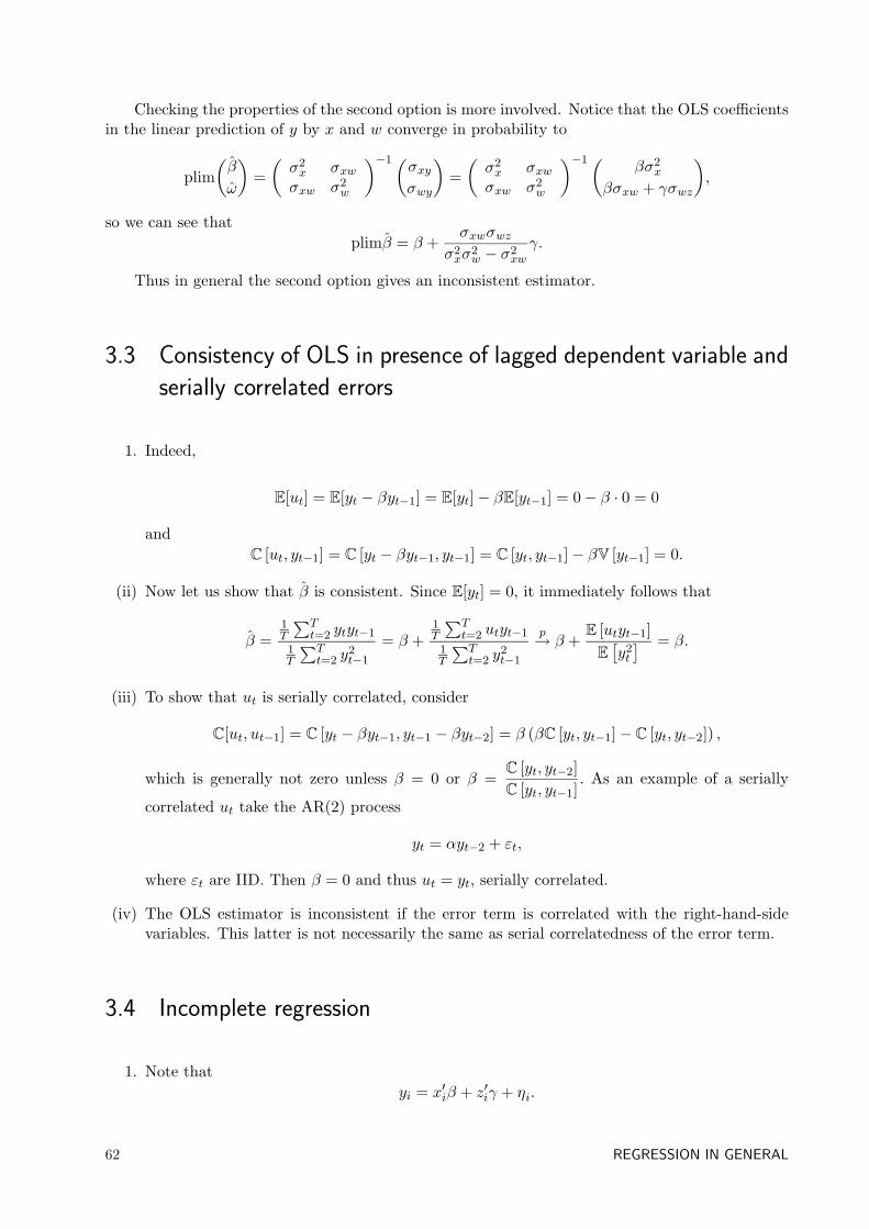
Checking the properties of the second option is more involved. Notice that the OLS coefficientsin the linear prediction of y by x and w converge in probability to
plim(β
ω
)=(σ2x σxwσxw σ2
w
)−1(σxyσwy
)=(σ2x σxwσxw σ2
w
)−1(βσ2
x
βσxw + γσwz
),
so we can see thatplimβ = β +
σxwσwzσ2xσ
2w − σ2
xw
γ.
Thus in general the second option gives an inconsistent estimator.
3.3 Consistency of OLS in presence of lagged dependent variable and
serially correlated errors
1. Indeed,
E[ut] = E[yt − βyt−1] = E[yt]− βE[yt−1] = 0− β · 0 = 0
andC [ut, yt−1] = C [yt − βyt−1, yt−1] = C [yt, yt−1]− βV [yt−1] = 0.
(ii) Now let us show that β is consistent. Since E[yt] = 0, it immediately follows that
β =1T
∑Tt=2 ytyt−1
1T
∑Tt=2 y
2t−1
= β +1T
∑Tt=2 utyt−1
1T
∑Tt=2 y
2t−1
p→ β +E [utyt−1]E
[y2t
] = β.
(iii) To show that ut is serially correlated, consider
C[ut, ut−1] = C [yt − βyt−1, yt−1 − βyt−2] = β (βC [yt, yt−1]− C [yt, yt−2]) ,
which is generally not zero unless β = 0 or β =C [yt, yt−2]C [yt, yt−1]
. As an example of a serially
correlated ut take the AR(2) process
yt = αyt−2 + εt,
where εt are IID. Then β = 0 and thus ut = yt, serially correlated.
(iv) The OLS estimator is inconsistent if the error term is correlated with the right-hand-sidevariables. This latter is not necessarily the same as serial correlatedness of the error term.
3.4 Incomplete regression
1. Note thatyi = x′iβ + z′iγ + ηi.
62 REGRESSION IN GENERAL
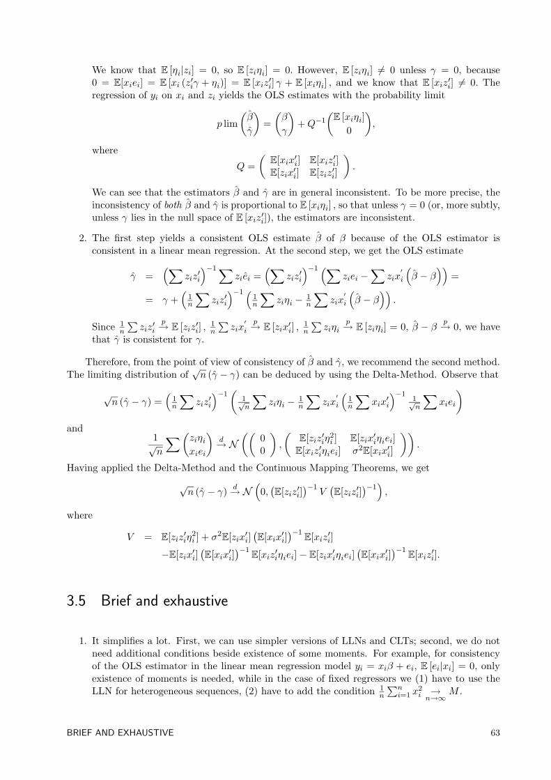
We know that E [ηi|zi] = 0, so E [ziηi] = 0. However, E [ziηi] 6= 0 unless γ = 0, because0 = E[xiei] = E [xi (z′iγ + ηi)] = E [xiz′i] γ + E [xiηi] , and we know that E [xiz′i] 6= 0. Theregression of yi on xi and zi yields the OLS estimates with the probability limit
p lim(β
γ
)=(β
γ
)+Q−1
(E [xiηi]
0
),
where
Q =(E[xix′i] E[xiz′i]E[zix′i] E[ziz′i]
).
We can see that the estimators β and γ are in general inconsistent. To be more precise, theinconsistency of both β and γ is proportional to E [xiηi] , so that unless γ = 0 (or, more subtly,unless γ lies in the null space of E [xiz′i]), the estimators are inconsistent.
2. The first step yields a consistent OLS estimate β of β because of the OLS estimator isconsistent in a linear mean regression. At the second step, we get the OLS estimate
γ =(∑
ziz′i
)−1∑ziei =
(∑ziz′i
)−1 (∑ziei −
∑zix
′i
(β − β
))=
= γ +(
1n
∑ziz′i
)−1 (1n
∑ziηi − 1
n
∑zix
′i
(β − β
)).
Since 1n
∑ziz′ip→ E [ziz′i] ,
1n
∑zix
′ip→ E [zix′i] ,
1n
∑ziηi
p→ E [ziηi] = 0, β − β p→ 0, we havethat γ is consistent for γ.
Therefore, from the point of view of consistency of β and γ, we recommend the second method.The limiting distribution of
√n (γ − γ) can be deduced by using the Delta-Method. Observe that
√n (γ − γ) =
(1n
∑ziz′i
)−1(
1√n
∑ziηi − 1
n
∑zix
′i
(1n
∑xix′i
)−11√n
∑xiei
)and
1√n
∑(ziηixiei
)d→ N
((00
),
(E[ziz′iη
2i ] E[zix′iηiei]
E[xiz′iηiei] σ2E[xix′i]
)).
Having applied the Delta-Method and the Continuous Mapping Theorems, we get
√n (γ − γ) d→ N
(0,(E[ziz′i]
)−1V(E[ziz′i]
)−1),
where
V = E[ziz′iη2i ] + σ2
E[zix′i](E[xix′i]
)−1E[xiz′i]
−E[zix′i](E[xix′i]
)−1E[xiz′iηiei]− E[zix′iηiei]
(E[xix′i]
)−1E[xiz′i].
3.5 Brief and exhaustive
1. It simplifies a lot. First, we can use simpler versions of LLNs and CLTs; second, we do notneed additional conditions beside existence of some moments. For example, for consistencyof the OLS estimator in the linear mean regression model yi = xiβ + ei, E [ei|xi] = 0, onlyexistence of moments is needed, while in the case of fixed regressors we (1) have to use theLLN for heterogeneous sequences, (2) have to add the condition 1
n
∑ni=1 x
2i →n→∞M .
BRIEF AND EXHAUSTIVE 63

2. The economist is probably right about treating the regressors as random if he has a randomsampling experiment. But his reasoning is completely ridiculous. For a sampled individual,his/her characteristics (whether true or false) are fixed; randomness arises from the fact thatthis individual is randomly selected.
3. E [x|z] = g(z) is a strictly increasing and continuous function, therefore g−1(·) exists andE [x|z] = γ is equivalent to z = g−1(γ). If E[y|z] = f(z), then E [y|E [x|z] = γ] = f(g−1(γ)).
4. Yes, one should use White’s formula, but not because σ2Q−1xx does not make sense. It does
make sense, but is irrelevant to calculation of the asymptotic variance of the OLS estimator,which in general takes the ”sandwich” form. It is not true that σ2 varies from observation toobservation, if by σ2 we mean unconditional variance of the error term.
64 REGRESSION IN GENERAL
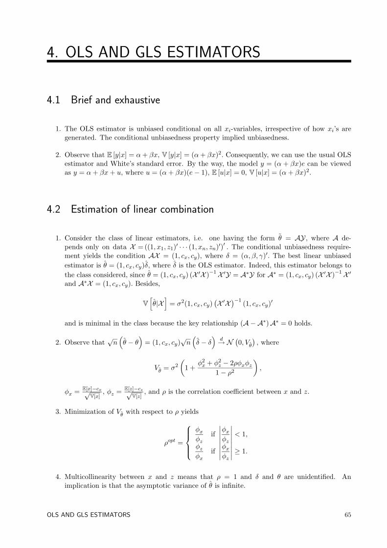
4. OLS AND GLS ESTIMATORS
4.1 Brief and exhaustive
1. The OLS estimator is unbiased conditional on all xi-variables, irrespective of how xi’s aregenerated. The conditional unbiasedness property implied unbiasedness.
2. Observe that E [y|x] = α+ βx, V [y|x] = (α+ βx)2. Consequently, we can use the usual OLSestimator and White’s standard error. By the way, the model y = (α + βx)e can be viewedas y = α+ βx+ u, where u = (α+ βx)(e− 1), E [u|x] = 0, V [u|x] = (α+ βx)2.
4.2 Estimation of linear combination
1. Consider the class of linear estimators, i.e. one having the form θ = AY, where A de-pends only on data X = ((1, x1, z1)′ · · · (1, xn, zn)′)′ . The conditional unbiasedness require-ment yields the condition AX = (1, cx, cy), where δ = (α, β, γ)′. The best linear unbiasedestimator is θ = (1, cx, cy)δ, where δ is the OLS estimator. Indeed, this estimator belongs tothe class considered, since θ = (1, cx, cy) (X ′X )−1X ′Y = A∗Y for A∗ = (1, cx, cy) (X ′X )−1X ′and A∗X = (1, cx, cy). Besides,
V
[θ|X
]= σ2(1, cx, cy)
(X ′X
)−1 (1, cx, cy)′
and is minimal in the class because the key relationship (A−A∗)A∗ = 0 holds.
2. Observe that√n(θ − θ
)= (1, cx, cy)
√n(δ − δ
)d→ N
(0, Vθ
), where
Vθ = σ2
(1 +
φ2x + φ2
z − 2ρφxφz1− ρ2
),
φx = E[x]−cx√V[x]
, φz = E[z]−cz√V[z]
, and ρ is the correlation coefficient between x and z.
3. Minimization of Vθ with respect to ρ yields
ρopt =
φxφz
if∣∣∣∣φxφz
∣∣∣∣ < 1,
φzφx
if∣∣∣∣φxφz
∣∣∣∣ ≥ 1.
4. Multicollinearity between x and z means that ρ = 1 and δ and θ are unidentified. Animplication is that the asymptotic variance of θ is infinite.
OLS AND GLS ESTIMATORS 65
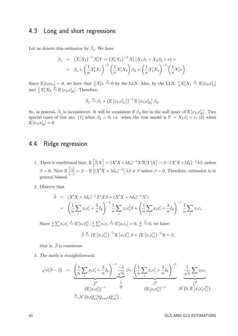
4.3 Long and short regressions
Let us denote this estimator by β1. We have
β1 =(X ′1X1
)−1X ′1Y =
(X ′1X1
)−1X ′1 (X1β1 +X2β2 + e) =
= β1 +(
1nX ′1X1
)−1( 1nX ′1X2
)β2 +
(1nX ′1X1
)−1( 1nX ′1e
).
Since E [eix1i] = 0, we have that 1nX′1e
p→ 0 by the LLN. Also, by the LLN, 1nX′1X1
p→ E [x1ix′1i]
and 1nX′1X2
p→ E [x1ix′2i] . Therefore,
β1p→ β1 +
(E
[x1ix
′1i
])−1E
[x1ix
′2i
]β2.
So, in general, β1 is inconsistent. It will be consistent if β2 lies in the null space of E [x1ix′2i] . Two
special cases of this are: (1) when β2 = 0, i.e. when the true model is Y = X1β1 + e; (2) whenE [x1ix
′2i] = 0.
4.4 Ridge regression
1. There is conditional bias: E[β|X
]= (X ′X+λIk)−1X ′E [Y |X] = β−(X ′X+λIk)−1λβ, unless
β = 0. Next E[β]
= β − E[(X ′X + λIk)−1
]λβ 6= β unless β = 0. Therefore, estimator is in
general biased.
2. Observe that
β = (X ′X + λIk)−1X ′Xβ + (X ′X + λIk)−1X ′ε
=
(1n
∑i
xix′i +
λ
nIk
)−11n
∑i
xix′iβ +
(1n
∑i
xix′i +
λ
nIk
)−11n
∑i
xiεi.
Since 1n
∑xix′ip→ E [xix′i] ,
1n
∑xiεi
p→ E [xiεi] = 0, λnp→ 0, we have:
βp→(E
[xix′i
])−1E
[xix′i
]β +
(E
[xix′i
])−1 0 = β,
that is, β is consistent.
3. The math is straightforward:
√n(β − β) =
(1n
∑i
xix′i +
λ
nIk
)−1
︸ ︷︷ ︸↓p
(E [xix′i])−1
−λ√n︸︷︷︸↓0
β+
(1n
∑i
xix′i +
λ
nIk
)−1
︸ ︷︷ ︸↓p
(E [xix′i])−1
1√n
∑i
xiεi︸ ︷︷ ︸↓d
N(0,E
[xix′iε
2i
])p→ N
(0, Q−1
xxQxxe2Q−1xx
).
66 OLS AND GLS ESTIMATORS
4. The conditional mean squared error criterion E[(β − β
)2|X]
can be used. For the OLS
estimator,
E
[(β − β
)2|X]
= V
[β]
= (X ′X)−1X ′ΩX(X ′X)−1.
For the ridge estimator,
E
[(β − β
)2|X]
=(X ′X + λIk
)−1 (X ′ΩX + λ2ββ′
) (X ′X + λIk
)−1
By the first order approximation, if λ is small, (X ′X + λIk)−1 ≈ (X ′X)−1(Ik − λ(X ′X)−1).Hence,
E
[(β − β
)2|X]≈ (X ′X)−1(I − λ(X ′X)−1)(X ′ΩX)(I − λ(X ′X)−1)(X ′X)−1
≈ E[(β − β)2]− λ(X ′X)−1[X ′ΩX(X ′X)−1 + (X ′X)−1X ′ΩX](X ′X)−1.
That is E[(β − β
)2|X]− E
[(β − β
)2|X]
= A, where A is likely to be positive definite.
Thus for small λ, β may be a preferable estimator to β according to the mean squared errorcriterion, despite its biasedness.
4.5 Exponential heteroskedasticity
1. At the first step, estimate consistently α and β. This can be done using the relationship
E
[y2|x
]= (x′β)2 + exp(x′β + α),
by using NLLS on this nonlinear mean regression, to get β. Then construct σ2i ≡ exp(x′iβ)
for all i (we don’t need exp(α) since it is just a multiplicative scalar that eventually cancelsout) and use these weights at the second step to construct a feasible GLS estimator of β:
β =
(1n
∑i
σ−2i xix
′i
)−11n
∑i
σ−2i xiyi.
2. The feasible GLS estimator is asymptotically efficient, since it is asymptotically equivalent toGLS. It is finite-sample inefficient, since we changed the weights from what GLS presumes.
4.6 OLS and GLS are identical
1. Evidently, E [Y |X] = Xβ and Σ = V [Y |X] = XΓX ′ + σ2In. Since the latter depends on X,we are in the heteroskedastic environment.
2. The OLS estimator isβ =
(X ′X
)−1X ′Y,
EXPONENTIAL HETEROSKEDASTICITY 67
and the GLS estimator isβ =
(X ′Σ−1X
)−1X ′Σ−1Y.
First, X ′e = X ′(Y −X (X ′X)−1X ′Y
)= X ′Y − X ′X (X ′X)−1X ′Y = X ′Y − X ′Y = 0.
Premultiply this by XΓ: XΓX ′e = 0. Add σ2e to both sides and combine the terms on theleft-hand side:
(XΓX ′ + σ2In
)e ≡ Σe = σ2e. Now predividing by matrix Σ gives e = σ2Σ−1e.
Premultiply once gain by X ′ to get 0 = X ′e = σ2X ′Σ−1e, or just X ′Σ−1e = 0. Recall nowwhat e is: X ′Σ−1Y = X ′Σ−1X (X ′X)−1X ′Y which implies β = β.
The fact that the two estimators are identical implies that all the statistics based on the twowill be identical and thus have the same distribution.
3. Evidently, in this model the coincidence of the two estimators gives unambiguous superiorityof the OLS estimator. In spite of heteroskedasticity, it is efficient in the class of linear unbiasedestimators, since it coincides with GLS. The GLS estimator is worse since its feasible versionrequires estimation of Σ, while the OLS estimator does not. Additional estimation of Σ addsnoise which may spoil finite sample performance of the GLS estimator. But all this is nottypical for ranking OLS and GLS estimators and is a result of a special form of matrix Σ.
4.7 OLS and GLS are equivalent
1. When ΣX = XΘ, we have X ′ΣX = X ′XΘ and Σ−1X = XΘ−1, so that
V
[β|X
]=(X ′X
)−1X ′ΣX
(X ′X
)−1 = Θ(X ′X
)−1
andV
[β|X
]=(X ′Σ−1X
)−1 =(X ′XΘ−1
)−1 = Θ(X ′X
)−1.
2. In this example,
Σ = σ2
1 ρ · · · ρρ 1 · · · ρ...
.... . .
...ρ ρ · · · 1
,and ΣX = σ2(1 + ρ(n− 1)) · (1, 1, · · · , 1)′ = XΘ, where
Θ = σ2(1 + ρ(n− 1)).
Thus one does not need to use GLS but instead do OLS to achieve the same finite-sampleefficiency.
4.8 Equicorrelated observations
This is essentially a repetition of the second part of the previous problem, from which it followsthat under the circumstances xn the best linear conditionally (on a constant which is the same asunconditionally) unbiased estimator of θ because of coincidence of its variance with that of the GLS
68 OLS AND GLS ESTIMATORS
estimator. Appealing to the case when |γ| > 1 (which is tempting because then the variance of xnis larger than that of, say, x1) is invalid, because it is ruled out by the Cauchy-Schwartz inequality.
One cannot appeal to the usual LLNs because x is non-ergodic. The variance of xn is V [xn] =1n · 1 + n−1
n · γ → γ as n → ∞, so the estimator xn is in general inconsistent (except in the casewhen γ = 0). For an example of inconsistent xn, assume that γ > 0 and consider the followingconstruct: ui = ε+ ς i, where ς i ∼ IID(0, 1− γ) and ε ∼ (0, γ) independent of ς i for all i. Then thecorrelation structure is exactly as in the problem, and 1
n
∑ui
p→ ε, a random nonzero limit.
EQUICORRELATED OBSERVATIONS 69

70 OLS AND GLS ESTIMATORS
5. IV AND 2SLS ESTIMATORS
5.1 Instrumental variables in ARMA models
Give brief but exhaustive answers to the following short questions.
1. The instrument xt−j is scalar, the parameter is scalar, so there is exact identification. Theinstrument is obviously valid. The asymptotic variance of the just identifying IV estimator ofa scalar parameter under homoskedasticity is Vxt−j = σ2Q−2
xz Qzz. Let us calculate all pieces:
Qzz = E
[x2t−j
]= V [xt] = σ2
(1− ρ2
)−1 ; Qxz = E [xt−1xt−j ] = C [xt−1, xt−j ] = ρj−1V [xt] =
σ2ρj−1(1− ρ2
)−1. Thus, Vxt−j = ρ2−2j
(1− ρ2
). It is monotonically declining in j, so this
suggests that the optimal instrument must be xt−1. Although this is not a proof of the fact,the optimal instrument is indeed xt−1.. The result makes sense, since the last observation ismost informative and embeds all information in all the other instruments.
2. It is possible to use as instruments lags of yt starting from yt−2 back to the past. The regressoryt−1 will not do as it is correlated with the error term through et−1. Among yt−2, yt−3, · · · thefirst one deserves more attention, since, intuitively, it contains more information than oldervalues of yt.
5.2 Inappropriate 2SLS
1. Since E[u] = 0, we have E [y] = αE[z2], so α is identified as long as z is not deterministic
zero. The analog estimator is
α =
(1n
∑i
z2i
)−11n
∑i
yi.
Since E[v] = 0, we have E[z] = πE[x], so π is identified as long as x is not centered aroundzero. The analog estimator is
π =
(1n
∑i
xi
)−11n
∑i
zi.
Since Σ does not depend on xi, we have Σ = V
(uivi
), so Σ is identified since both u and v
are identified. The analog estimator is
Σ =1n
∑i
(uivi
)(uivi
)′,
where ui = yi − αz2i and vi = zi − πxi.
IV AND 2SLS ESTIMATORS 71
2. The estimator satisfies
α =
(1n
∑i
z4i
)−11n
∑i
z2i yi =
(π4 1n
∑i
x4i
)−1
π2 1n
∑i
x2i yi.
We know that 1n
∑i x
4i
p→ E
[x4], 1n
∑i x
2i yi = απ2 1
n
∑i x
4i + 2απ 1
n
∑i x
3i vi + α 1
n
∑i x
2i v
2i +
1n
∑i x
2iui
p→ απ2E
[x4]
+ αE[x2v2
], and π
p→ π. Therefore,
αp→ α+
α
π2
E
[x2v2
]E [x4]
6= α.
3. Evidently, we should fit the estimate of the square of zi, instead of the square of the estimate.To do this, note that the second equation and properties of the model imply
E
[z2i |xi
]= E
[(πxi + vi)2|xi
]= π2x2
i + 2E [πxivi|xi] + E[v2i |xi
]= π2x2
i + σ2v.
That is, we have a linear mean regression of z2 on x2 and a constant. Therefore, in thefirst stage we should regress z2 on x2 and a constant and construct z2
i = π2x2i + σ2
v, and inthe second stage, we should regress yi on z2
i . Consistency of this estimator follows from thetheory of 2SLS, when we treat z2 as a right hand side variable, not z.
5.3 Inconsistency under alternative
We are interesting in the question whether the t-statistics can be used to check H0 : β = 0. Inorder to answer this question we have to investigate the asymptotic properties of β. First of all,β = β +
(∑ni=1 z
2i
)−1∑ni=1 ziεi →p 0, since under the null,
n∑i=1
ziεip→ E [(x+ v)(u− βv)] = −βη2 = 0.
It is straightforward to show that under the null the conventional standard error correctly estimates(i.e. if correctly normalized, is consistent for) the asymptotic variance of β . That is, under thenull, tβ
d→ N (0, 1) , which means that we can use the conventional t-statistics for testing H0.
5.4 Trade and growth
1. The economic rationale for uncorrelatedness is that the variables Pi and Si are exogenousand are unaffected by what’s going on in the economy, and on the other hand, hardly canthey affect the income in other ways than through the trade. To estimate (5.1), we can usejust-identifying IV estimation, where the vector of right-hand-side variables is x = (1, T,W )′
and the instrument vector is z = (1, P, S)′. (Note: the full answer should include the detailsof performing the estimation up to getting the standard errors).
2. When data on within-country trade are not available, none of the coefficients in (5.1) isidentifiable without further assumptions. In general, neither of the available variables canserve as instruments for T in (5.1) where the composite error term is γWi + εi.
72 IV AND 2SLS ESTIMATORS
3. We can exploit the assumption that Pi is uncorrelated with the error term in (5.3). Substitute(5.3) into (5.1) to get
log Yi = (α+ γη) + βTi + γλSi + (γνi + εi) .
Now we see that Si and Pi are uncorrelated with the composite error term γνi + εi due totheir exogeneity and due to their uncorrelatedness with νi which follows from the additionalassumption and νi being the best linear prediction error in (5.3). (Note: again, the full answershould include the details of performing the estimation up to getting the standard errors, atleast). As for the coefficients of (5.1), only β will be consistently estimated, but not α or γ.
4. In general, for this model the OLS is inconsistent, and the IV method is consistent. Thus, thediscrepancy may be due to the different probability limits of the two estimators. The fact thatthe IV estimates are larger says that probably Let θIV
p→ θ and θOLSp→ θ + a, a < 0. Then
for large samples, θIV ≈ θ and θOLS ≈ θ + a. The difference is a which is (E [xx′])−1E[xe].
Since (E [xx′])−1 is positive definite, a < 0 means that the regressors tend to be negativelycorrelated with the error term. In the present context this means that the trade variables arenegatively correlated with other influences on income.
TRADE AND GROWTH 73

74 IV AND 2SLS ESTIMATORS
6. EXTREMUM ESTIMATORS
6.1 Extremum estimators
Part 1. The analog estimator is
β =arg maxb∈B
1n
n∑i=1
f(zi, b). (6.1)
Assume that:
1. βp→ β;
2. β is an interior point of the compact set B (i. e. β is contained in B with its open neighbor-hood);
3. f(z, b) is a twice continuously differentiable function of b for almost all z;
4. the derivatives ∂f(z,b)∂b and ∂2f(z,b)
∂b∂b′ satisfy the ULLN condition in B;
5. ∀b ∈ B there exist and are finite the moments E [|f(z, b)|] , E[∥∥∥∂f(z,b)
∂b
∥∥∥] and E[∥∥∥∂2f(z,b)
∂b∂b′
∥∥∥];6. there exists finite E [fbf ′b] ≡ E
[∂f(z,β)∂b
∂f(z,β)∂b′
], and matrix E [fbb] ≡ E
[∂2f(z,β)∂b∂b′
]is non-
degenerate.
Then β is asymptotically normal with asymptotic variance given below in (6.3). To see thiswrite the FOC for an interior solution of problem (6.1) and expand the first derivative aroundb = β:
0 =∂
∂b
(1n
n∑i=1
f(zi, β)
)=
∂
∂b
(1n
n∑i=1
f(zi, β)
)+
∂2
∂b∂b′
(1n
n∑i=1
f(zi, β∗)
)(β − β), (6.2)
where β∗s ∈ [βs, βs] and β∗ may be different in different equations of (6.2). In particular, β∗p→ β.
From here,√n(β − β) = −
(1n
n∑i=1
∂2f(zi, β∗)∂b∂b′
)−11√n
n∑i=1
∂f(zi, β)∂b
.
By the ULLN condition for∂2f(z,b)∂b∂b′ one has
1n
n∑i=1
∂2f(zi, β∗)∂b∂b′
p→ E [fbb] .
By the CLT, applicable to independent random variables,
1√n
n∑i=1
∂f(zi, β)∂b
d→ N(0,E
[fbf′b
]).
EXTREMUM ESTIMATORS 75
The last equality uses the FOC for the extremum problem for β: E[∂f(zi,β)
∂b
]= 0. Thus,
√n(β − β) d→ N
(0,(
(E [fbb])−1E
[fbf′b
](E [fbb])
−1)−1
). (6.3)
Part 2. Let E [y|x] = g(x, β), σ2(x) ≡ E[(y − g(x, β))2
]. The NLLS and WNLLS estimators
are extremum estimators with
f1(x, y, b) = −12
(y − g(x, b))2 for NLLS,
and
f2(x, y, b) = −12
(y − g(x, b))2
σ2(x)=f1(x, y, b)σ2(x)
for WNLLS.
It was shown in class that√n(βNLLS − β) d→ N
(0, Q−1
gg Qgge2Q−1gg
),√n(βWNLLS − β) d→ N
(0, Q gg
σ2
),
where
Qgg = E
[gb(x, β)gb(x, β)′
],
Qgge2 = E
[gb(x, β)gb(x, β)′(y − g(x, β))2
],
Q gg
σ2= E
[gb(x, β)gb(x, β)′/σ2(x)
].
This coincides with (6.3) since
∂f1(x, β)∂b
= (y − g(x, β))gb(x, β)
and∂2f1(x, β)∂b∂b′
= (y − g(x, β))gbb(x, β)− gb(x, β)gb(x, β)′,
and E [(y − g(x, β))gbb(x, β)] = E [E [y − g(x, β)|x] gbb(x, β)] = 0. In fact, we have E [f1bf′1b] = Qgge2 ,
−E [f1bb] = Qgg, E [f2bf′2b] = −E [f2bb] = Q gg
σ2.
It is worth noting that under the ID-condition for NLLS/WNLLS estimators the solution ofcorresponding extremum problem in population is unique and equals β.
6.2 Regression on constant
For the first estimator use standard LLN and CLT:
β1 =1n
n∑i=1
yip→ E[yi] = β (consistency),
√n(β1 − β) =
1√n
n∑i=1
eid→ N (0,V[ei]) = N
(0, β2
)(asymptotic normality).
Consider
β2 =arg minb
log b2 +
1nb2
n∑i=1
(yi − b)2
. (6.4)
76 EXTREMUM ESTIMATORS
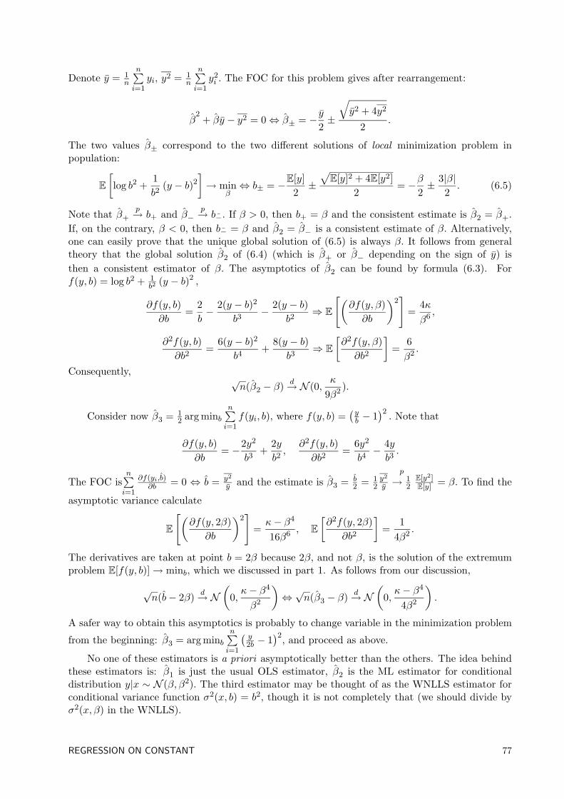
Denote y = 1n
n∑i=1
yi, y2 = 1n
n∑i=1
y2i . The FOC for this problem gives after rearrangement:
β2
+ βy − y2 = 0⇔ β± = − y2±
√y2 + 4y2
2.
The two values β± correspond to the two different solutions of local minimization problem inpopulation:
E
[log b2 +
1b2
(y − b)2
]→ min
β⇔ b± = −E[y]
2±√E[y]2 + 4E[y2]
2= −β
2± 3|β|
2. (6.5)
Note that β+p→ b+ and β−
p→ b−. If β > 0, then b+ = β and the consistent estimate is β2 = β+.
If, on the contrary, β < 0, then b− = β and β2 = β− is a consistent estimate of β. Alternatively,one can easily prove that the unique global solution of (6.5) is always β. It follows from generaltheory that the global solution β2 of (6.4) (which is β+ or β− depending on the sign of y) isthen a consistent estimator of β. The asymptotics of β2 can be found by formula (6.3). Forf(y, b) = log b2 + 1
b2(y − b)2 ,
∂f(y, b)∂b
=2b− 2(y − b)2
b3− 2(y − b)
b2⇒ E
[(∂f(y, β)∂b
)2]
=4κβ6 ,
∂2f(y, b)∂b2
=6(y − b)2
b4+
8(y − b)b3
⇒ E
[∂2f(y, β)∂b2
]=
6β2 .
Consequently,√n(β2 − β) d→ N (0,
κ
9β2 ).
Consider now β3 = 12 arg minb
n∑i=1
f(yi, b), where f(y, b) =(yb − 1
)2. Note that
∂f(y, b)∂b
= −2y2
b3+
2yb2,
∂2f(y, b)∂b2
=6y2
b4− 4yb3.
The FOC isn∑i=1
∂f(yi,b)∂b = 0 ⇔ b = y2
y and the estimate is β3 = b2 = 1
2y2
y
p
→ 12E[y2]E[y] = β. To find the
asymptotic variance calculate
E
[(∂f(y, 2β)
∂b
)2]
=κ− β4
16β6 , E
[∂2f(y, 2β)
∂b2
]=
14β2 .
The derivatives are taken at point b = 2β because 2β, and not β, is the solution of the extremumproblem E[f(y, b)]→ minb, which we discussed in part 1. As follows from our discussion,
√n(b− 2β) d→ N
(0,κ− β4
β2
)⇔√n(β3 − β) d→ N
(0,κ− β4
4β2
).
A safer way to obtain this asymptotics is probably to change variable in the minimization problem
from the beginning: β3 = arg minbn∑i=1
( y2b − 1
)2, and proceed as above.
No one of these estimators is a priori asymptotically better than the others. The idea behindthese estimators is: β1 is just the usual OLS estimator, β2 is the ML estimator for conditionaldistribution y|x ∼ N (β, β2). The third estimator may be thought of as the WNLLS estimator forconditional variance function σ2(x, b) = b2, though it is not completely that (we should divide byσ2(x, β) in the WNLLS).
REGRESSION ON CONSTANT 77
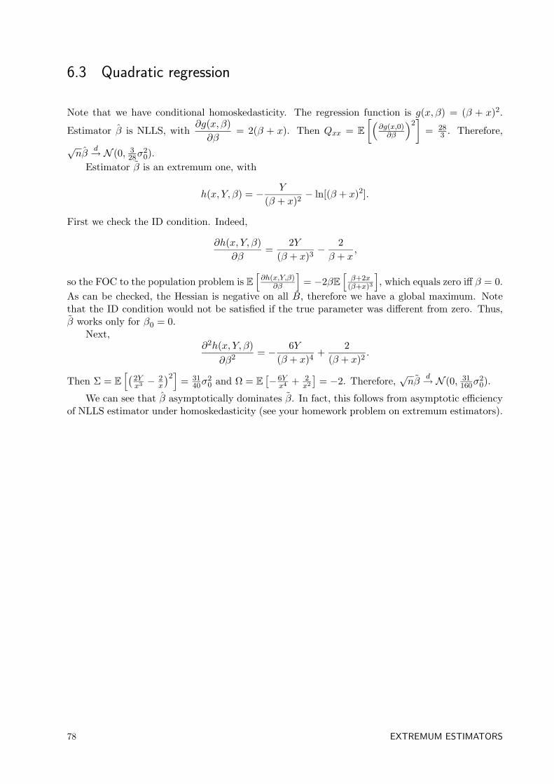
6.3 Quadratic regression
Note that we have conditional homoskedasticity. The regression function is g(x, β) = (β + x)2.
Estimator β is NLLS, with∂g(x, β)∂β
= 2(β + x). Then Qxx = E
[(∂g(x,0)∂β
)2]
= 283 . Therefore,
√nβ
d→ N (0, 328σ
20).
Estimator β is an extremum one, with
h(x, Y, β) = − Y
(β + x)2− ln[(β + x)2].
First we check the ID condition. Indeed,
∂h(x, Y, β)∂β
=2Y
(β + x)3− 2β + x
,
so the FOC to the population problem is E[∂h(x,Y,β)
∂β
]= −2βE
[β+2x
(β+x)3
], which equals zero iff β = 0.
As can be checked, the Hessian is negative on all B, therefore we have a global maximum. Notethat the ID condition would not be satisfied if the true parameter was different from zero. Thus,β works only for β0 = 0.
Next,∂2h(x, Y, β)
∂β2 = − 6Y(β + x)4
+2
(β + x)2.
Then Σ = E
[(2Yx3 − 2
x
)2] = 3140σ
20 and Ω = E
[−6Yx4 + 2
x2
]= −2. Therefore,
√nβ
d→ N (0, 31160σ
20).
We can see that β asymptotically dominates β. In fact, this follows from asymptotic efficiencyof NLLS estimator under homoskedasticity (see your homework problem on extremum estimators).
78 EXTREMUM ESTIMATORS
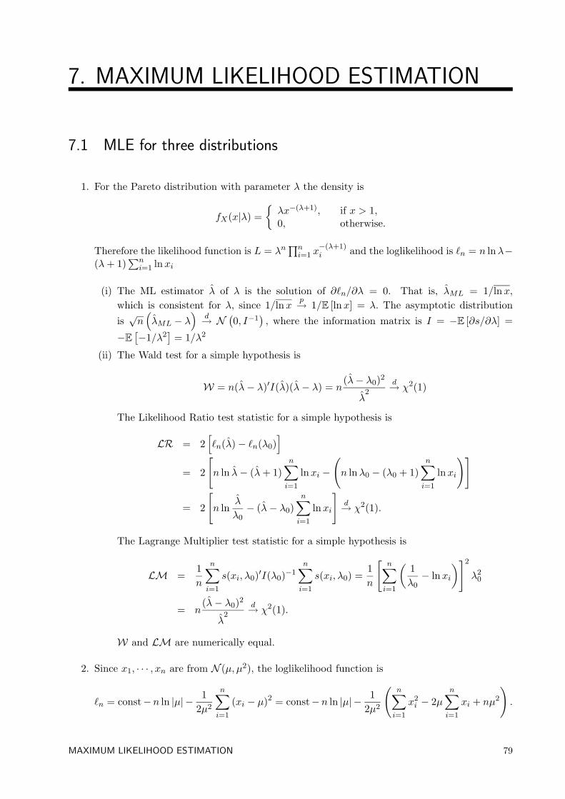
7. MAXIMUM LIKELIHOOD ESTIMATION
7.1 MLE for three distributions
1. For the Pareto distribution with parameter λ the density is
fX(x|λ) =λx−(λ+1), if x > 1,0, otherwise.
Therefore the likelihood function is L = λn∏ni=1 x
−(λ+1)i and the loglikelihood is `n = n lnλ−
(λ+ 1)∑n
i=1 lnxi
(i) The ML estimator λ of λ is the solution of ∂`n/∂λ = 0. That is, λML = 1/lnx,which is consistent for λ, since 1/lnx
p→ 1/E [lnx] = λ. The asymptotic distributionis√n(λML − λ
)d→ N
(0, I−1
), where the information matrix is I = −E [∂s/∂λ] =
−E[−1/λ2
]= 1/λ2
(ii) The Wald test for a simple hypothesis is
W = n(λ− λ)′I(λ)(λ− λ) = n(λ− λ0)2
λ2
d→ χ2(1)
The Likelihood Ratio test statistic for a simple hypothesis is
LR = 2[`n(λ)− `n(λ0)
]= 2
[n ln λ− (λ+ 1)
n∑i=1
lnxi −
(n lnλ0 − (λ0 + 1)
n∑i=1
lnxi
)]
= 2
[n ln
λ
λ0− (λ− λ0)
n∑i=1
lnxi
]d→ χ2(1).
The Lagrange Multiplier test statistic for a simple hypothesis is
LM =1n
n∑i=1
s(xi, λ0)′I(λ0)−1n∑i=1
s(xi, λ0) =1n
[n∑i=1
(1λ0− lnxi
)]2
λ20
= n(λ− λ0)2
λ2
d→ χ2(1).
W and LM are numerically equal.
2. Since x1, · · · , xn are from N (µ, µ2), the loglikelihood function is
`n = const−n ln |µ| − 12µ2
n∑i=1
(xi − µ)2 = const−n ln |µ| − 12µ2
(n∑i=1
x2i − 2µ
n∑i=1
xi + nµ2
).
MAXIMUM LIKELIHOOD ESTIMATION 79
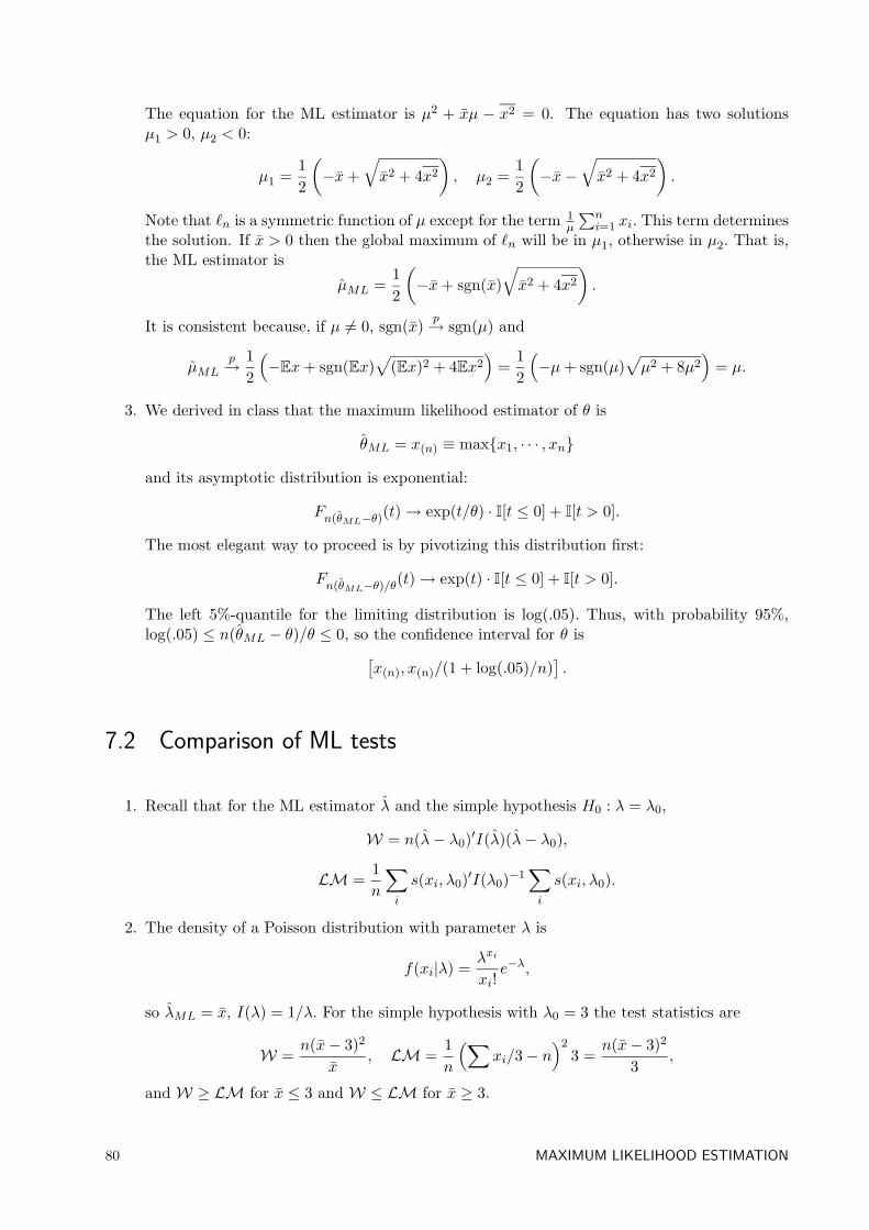
The equation for the ML estimator is µ2 + xµ − x2 = 0. The equation has two solutionsµ1 > 0, µ2 < 0:
µ1 =12
(−x+
√x2 + 4x2
), µ2 =
12
(−x−
√x2 + 4x2
).
Note that `n is a symmetric function of µ except for the term 1µ
∑ni=1 xi. This term determines
the solution. If x > 0 then the global maximum of `n will be in µ1, otherwise in µ2. That is,the ML estimator is
µML =12
(−x+ sgn(x)
√x2 + 4x2
).
It is consistent because, if µ 6= 0, sgn(x)p→ sgn(µ) and
µMLp→ 1
2
(−Ex+ sgn(Ex)
√(Ex)2 + 4Ex2
)=
12
(−µ+ sgn(µ)
√µ2 + 8µ2
)= µ.
3. We derived in class that the maximum likelihood estimator of θ is
θML = x(n) ≡ maxx1, · · · , xn
and its asymptotic distribution is exponential:
Fn(θML−θ)(t)→ exp(t/θ) · I[t ≤ 0] + I[t > 0].
The most elegant way to proceed is by pivotizing this distribution first:
Fn(θML−θ)/θ(t)→ exp(t) · I[t ≤ 0] + I[t > 0].
The left 5%-quantile for the limiting distribution is log(.05). Thus, with probability 95%,log(.05) ≤ n(θML − θ)/θ ≤ 0, so the confidence interval for θ is[
x(n), x(n)/(1 + log(.05)/n)].
7.2 Comparison of ML tests
1. Recall that for the ML estimator λ and the simple hypothesis H0 : λ = λ0,
W = n(λ− λ0)′I(λ)(λ− λ0),
LM =1n
∑i
s(xi, λ0)′I(λ0)−1∑i
s(xi, λ0).
2. The density of a Poisson distribution with parameter λ is
f(xi|λ) =λxi
xi!e−λ,
so λML = x, I(λ) = 1/λ. For the simple hypothesis with λ0 = 3 the test statistics are
W =n(x− 3)2
x, LM =
1n
(∑xi/3− n
)23 =
n(x− 3)2
3,
and W ≥ LM for x ≤ 3 and W ≤ LM for x ≥ 3.
80 MAXIMUM LIKELIHOOD ESTIMATION
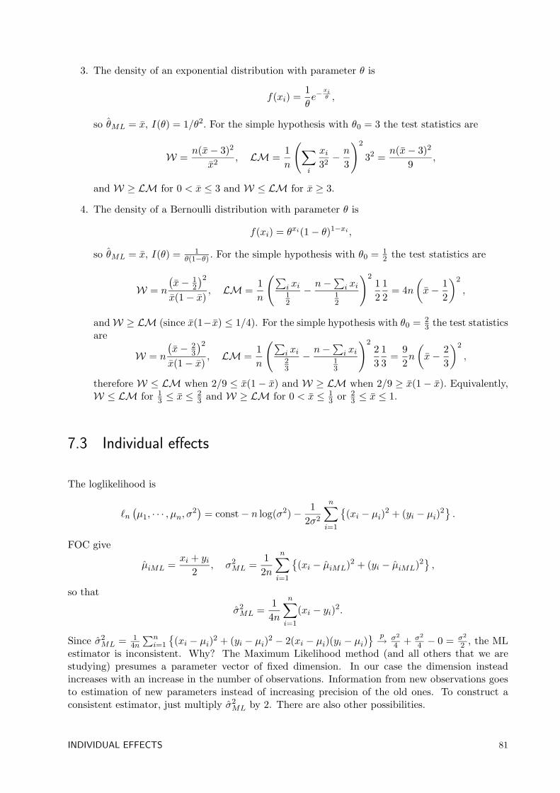
3. The density of an exponential distribution with parameter θ is
f(xi) =1θe−
xiθ ,
so θML = x, I(θ) = 1/θ2. For the simple hypothesis with θ0 = 3 the test statistics are
W =n(x− 3)2
x2, LM =
1n
(∑i
xi32− n
3
)2
32 =n(x− 3)2
9,
and W ≥ LM for 0 < x ≤ 3 and W ≤ LM for x ≥ 3.
4. The density of a Bernoulli distribution with parameter θ is
f(xi) = θxi(1− θ)1−xi ,
so θML = x, I(θ) = 1θ(1−θ) . For the simple hypothesis with θ0 = 1
2 the test statistics are
W = n
(x− 1
2
)2x(1− x)
, LM =1n
(∑i xi12
−n−
∑i xi
12
)212
12
= 4n(x− 1
2
)2
,
andW ≥ LM (since x(1−x) ≤ 1/4). For the simple hypothesis with θ0 = 23 the test statistics
are
W = n
(x− 2
3
)2x(1− x)
, LM =1n
(∑i xi23
−n−
∑i xi
13
)223
13
=92n
(x− 2
3
)2
,
therefore W ≤ LM when 2/9 ≤ x(1− x) and W ≥ LM when 2/9 ≥ x(1− x). Equivalently,W ≤ LM for 1
3 ≤ x ≤23 and W ≥ LM for 0 < x ≤ 1
3 or 23 ≤ x ≤ 1.
7.3 Individual effects
The loglikelihood is
`n(µ1, · · · , µn, σ2
)= const− n log(σ2)− 1
2σ2
n∑i=1
(xi − µi)2 + (yi − µi)2
.
FOC give
µiML =xi + yi
2, σ2
ML =1
2n
n∑i=1
(xi − µiML)2 + (yi − µiML)2
,
so that
σ2ML =
14n
n∑i=1
(xi − yi)2.
Since σ2ML = 1
4n
∑ni=1
(xi − µi)2 + (yi − µi)2 − 2(xi − µi)(yi − µi)
p→ σ2
4 + σ2
4 − 0 = σ2
2 , the MLestimator is inconsistent. Why? The Maximum Likelihood method (and all others that we arestudying) presumes a parameter vector of fixed dimension. In our case the dimension insteadincreases with an increase in the number of observations. Information from new observations goesto estimation of new parameters instead of increasing precision of the old ones. To construct aconsistent estimator, just multiply σ2
ML by 2. There are also other possibilities.
INDIVIDUAL EFFECTS 81
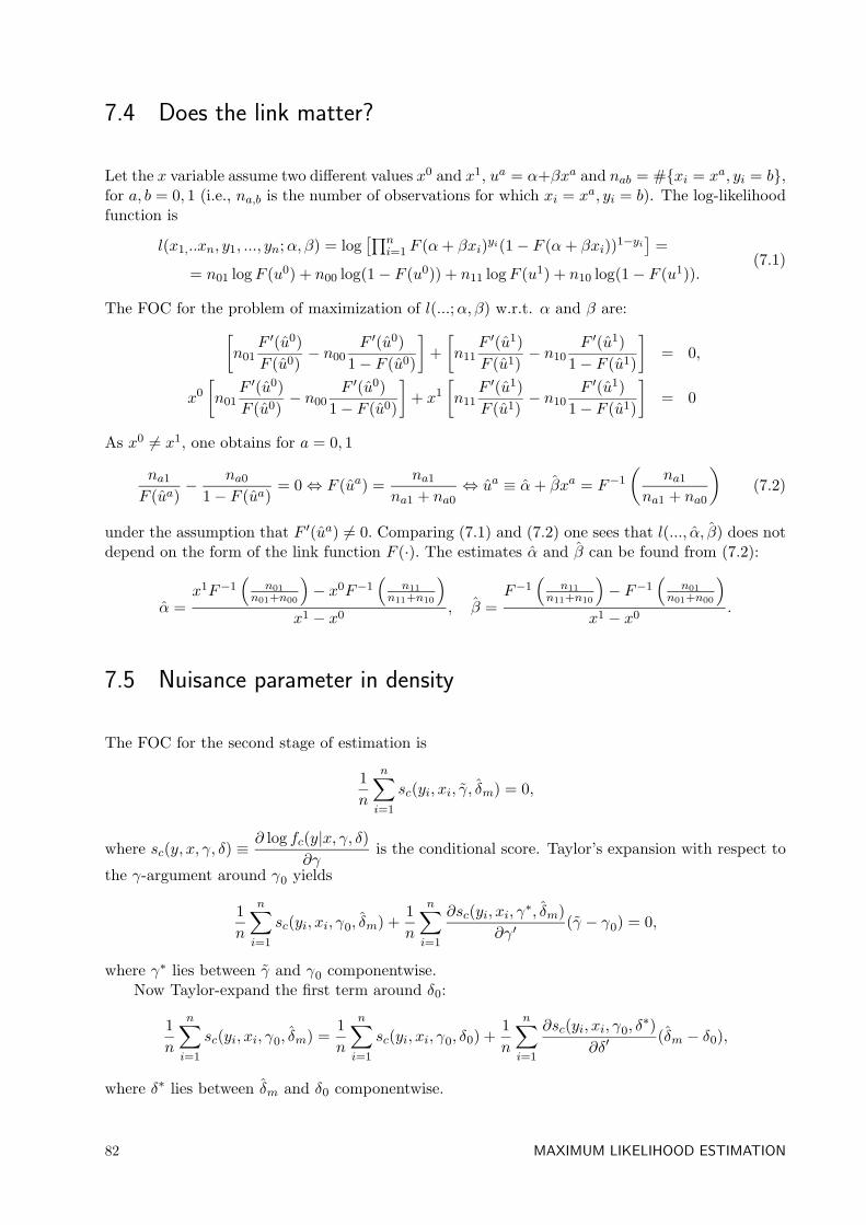
7.4 Does the link matter?
Let the x variable assume two different values x0 and x1, ua = α+βxa and nab = #xi = xa, yi = b,for a, b = 0, 1 (i.e., na,b is the number of observations for which xi = xa, yi = b). The log-likelihoodfunction is
l(x1,..xn, y1, ..., yn;α, β) = log[∏n
i=1 F (α+ βxi)yi(1− F (α+ βxi))1−yi]
=
= n01 logF (u0) + n00 log(1− F (u0)) + n11 logF (u1) + n10 log(1− F (u1)).(7.1)
The FOC for the problem of maximization of l(...;α, β) w.r.t. α and β are:[n01
F ′(u0)F (u0)
− n00F ′(u0)
1− F (u0)
]+[n11
F ′(u1)F (u1)
− n10F ′(u1)
1− F (u1)
]= 0,
x0
[n01
F ′(u0)F (u0)
− n00F ′(u0)
1− F (u0)
]+ x1
[n11
F ′(u1)F (u1)
− n10F ′(u1)
1− F (u1)
]= 0
As x0 6= x1, one obtains for a = 0, 1
na1
F (ua)− na0
1− F (ua)= 0⇔ F (ua) =
na1
na1 + na0⇔ ua ≡ α+ βxa = F−1
(na1
na1 + na0
)(7.2)
under the assumption that F ′(ua) 6= 0. Comparing (7.1) and (7.2) one sees that l(..., α, β) does notdepend on the form of the link function F (·). The estimates α and β can be found from (7.2):
α =x1F−1
(n01
n01+n00
)− x0F−1
(n11
n11+n10
)x1 − x0
, β =F−1
(n11
n11+n10
)− F−1
(n01
n01+n00
)x1 − x0
.
7.5 Nuisance parameter in density
The FOC for the second stage of estimation is
1n
n∑i=1
sc(yi, xi, γ, δm) = 0,
where sc(y, x, γ, δ) ≡∂ log fc(y|x, γ, δ)
∂γis the conditional score. Taylor’s expansion with respect to
the γ-argument around γ0 yields
1n
n∑i=1
sc(yi, xi, γ0, δm) +1n
n∑i=1
∂sc(yi, xi, γ∗, δm)∂γ′
(γ − γ0) = 0,
where γ∗ lies between γ and γ0 componentwise.Now Taylor-expand the first term around δ0:
1n
n∑i=1
sc(yi, xi, γ0, δm) =1n
n∑i=1
sc(yi, xi, γ0, δ0) +1n
n∑i=1
∂sc(yi, xi, γ0, δ∗)
∂δ′(δm − δ0),
where δ∗ lies between δm and δ0 componentwise.
82 MAXIMUM LIKELIHOOD ESTIMATION
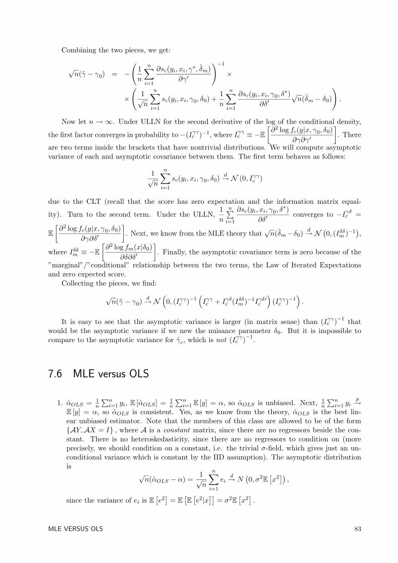
Combining the two pieces, we get:
√n(γ − γ0) = −
(1n
n∑i=1
∂sc(yi, xi, γ∗, δm)∂γ′
)−1
×
×
(1√n
n∑i=1
sc(yi, xi, γ0, δ0) +1n
n∑i=1
∂sc(yi, xi, γ0, δ∗)
∂δ′√n(δm − δ0)
).
Now let n → ∞. Under ULLN for the second derivative of the log of the conditional density,
the first factor converges in probability to −(Iγγc )−1, where Iγγc ≡ −E[∂2 log fc(y|x, γ0, δ0)
∂γ∂γ′
]. There
are two terms inside the brackets that have nontrivial distributions. We will compute asymptoticvariance of each and asymptotic covariance between them. The first term behaves as follows:
1√n
n∑i=1
sc(yi, xi, γ0, δ0) d→ N (0, Iγγc )
due to the CLT (recall that the score has zero expectation and the information matrix equal-
ity). Turn to the second term. Under the ULLN,1n
n∑i=1
∂sc(yi, xi, γ0, δ∗)
∂δ′converges to −Iγδc =
E
[∂2 log fc(y|x, γ0, δ0)
∂γ∂δ′
]. Next, we know from the MLE theory that
√n(δm−δ0) d→ N
(0, (Iδδm )−1
),
where Iδδm ≡ −E[∂2 log fm(x|δ0)
∂δ∂δ′
]. Finally, the asymptotic covariance term is zero because of the
”marginal”/”conditional” relationship between the two terms, the Law of Iterated Expectationsand zero expected score.
Collecting the pieces, we find:
√n(γ − γ0) d→ N
(0, (Iγγc )−1
(Iγγc + Iγδc (Iδδm )−1Iγδc
′)
(Iγγc )−1).
It is easy to see that the asymptotic variance is larger (in matrix sense) than (Iγγc )−1 thatwould be the asymptotic variance if we new the nuisance parameter δ0. But it is impossible tocompare to the asymptotic variance for γc, which is not (Iγγc )−1.
7.6 MLE versus OLS
1. αOLS = 1n
∑ni=1 yi, E [αOLS ] = 1
n
∑ni=1 E [y] = α, so αOLS is unbiased. Next, 1
n
∑ni=1 yi
p→E [y] = α, so αOLS is consistent. Yes, as we know from the theory, αOLS is the best lin-ear unbiased estimator. Note that the members of this class are allowed to be of the formAY,AX = I , where A is a constant matrix, since there are no regressors beside the con-stant. There is no heteroskedasticity, since there are no regressors to condition on (moreprecisely, we should condition on a constant, i.e. the trivial σ-field, which gives just an un-conditional variance which is constant by the IID assumption). The asymptotic distributionis
√n(αOLS − α) =
1√n
n∑i=1
eid→ N
(0, σ2
E
[x2]),
since the variance of ei is E[e2]
= E
[E
[e2|x
]]= σ2
E
[x2].
MLE VERSUS OLS 83
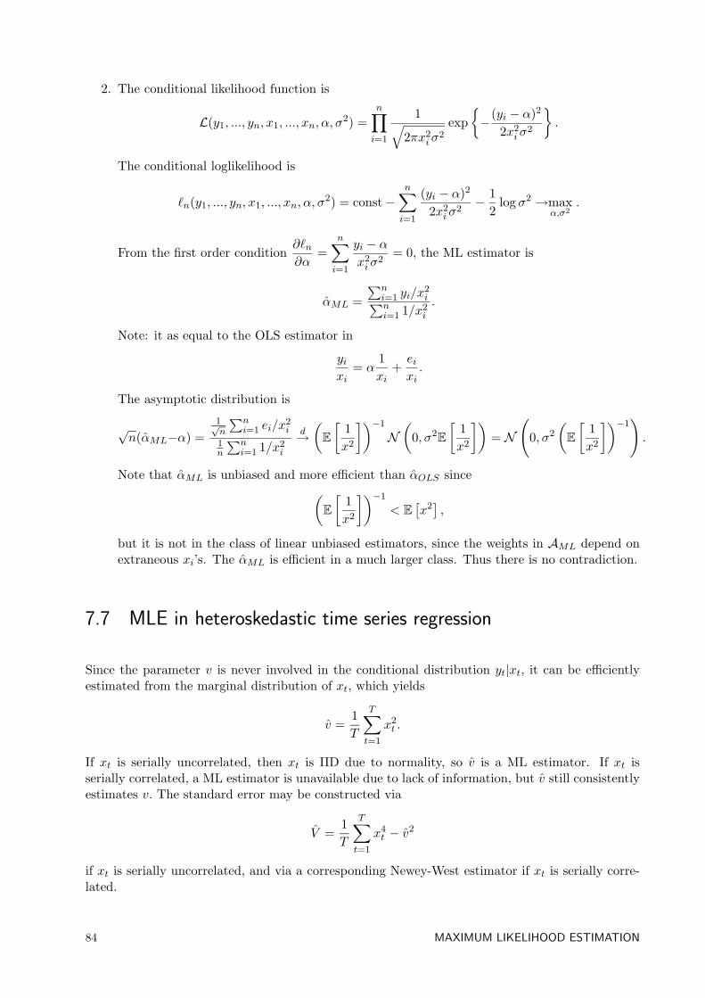
2. The conditional likelihood function is
L(y1, ..., yn, x1, ..., xn, α, σ2) =
n∏i=1
1√2πx2
iσ2
exp−(yi − α)2
2x2iσ
2
.
The conditional loglikelihood is
`n(y1, ..., yn, x1, ..., xn, α, σ2) = const−
n∑i=1
(yi − α)2
2x2iσ
2− 1
2log σ2 →max
α,σ2.
From the first order condition∂`n∂α
=n∑i=1
yi − αx2iσ
2= 0, the ML estimator is
αML =∑n
i=1 yi/x2i∑n
i=1 1/x2i
.
Note: it as equal to the OLS estimator in
yixi
= α1xi
+eixi.
The asymptotic distribution is
√n(αML−α) =
1√n
∑ni=1 ei/x
2i
1n
∑ni=1 1/x2
i
d→(E
[1x2
])−1
N(
0, σ2E
[1x2
])= N
(0, σ2
(E
[1x2
])−1).
Note that αML is unbiased and more efficient than αOLS since(E
[1x2
])−1
< E[x2],
but it is not in the class of linear unbiased estimators, since the weights in AML depend onextraneous xi’s. The αML is efficient in a much larger class. Thus there is no contradiction.
7.7 MLE in heteroskedastic time series regression
Since the parameter v is never involved in the conditional distribution yt|xt, it can be efficientlyestimated from the marginal distribution of xt, which yields
v =1T
T∑t=1
x2t .
If xt is serially uncorrelated, then xt is IID due to normality, so v is a ML estimator. If xt isserially correlated, a ML estimator is unavailable due to lack of information, but v still consistentlyestimates v. The standard error may be constructed via
V =1T
T∑t=1
x4t − v2
if xt is serially uncorrelated, and via a corresponding Newey-West estimator if xt is serially corre-lated.
84 MAXIMUM LIKELIHOOD ESTIMATION
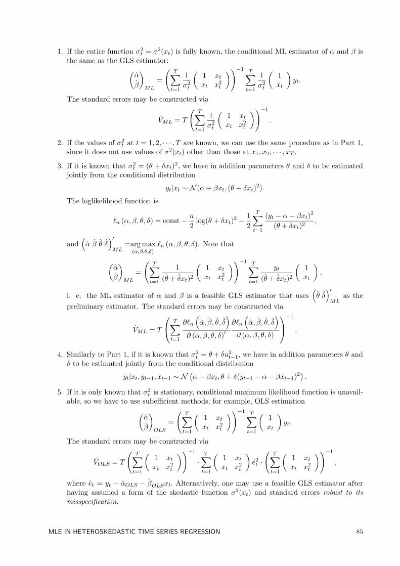
1. If the entire function σ2t = σ2(xt) is fully known, the conditional ML estimator of α and β is
the same as the GLS estimator:(α
β
)ML
=
(T∑t=1
1σ2t
(1 xtxt x2
t
))−1 T∑t=1
1σ2t
(1xt
)yt.
The standard errors may be constructed via
VML = T
(T∑t=1
1σ2t
(1 xtxt x2
t
))−1
.
2. If the values of σ2t at t = 1, 2, · · · , T are known, we can use the same procedure as in Part 1,
since it does not use values of σ2(xt) other than those at x1, x2, · · · , xT .
3. If it is known that σ2t = (θ + δxt)2, we have in addition parameters θ and δ to be estimated
jointly from the conditional distribution
yt|xt ∼ N (α+ βxt, (θ + δxt)2).
The loglikelihood function is
`n (α, β, θ, δ) = const− n
2log(θ + δxt)2 − 1
2
T∑t=1
(yt − α− βxt)2
(θ + δxt)2,
and(α β θ δ
)′ML
=arg max(α,β,θ,δ)
`n (α, β, θ, δ). Note that
(α
β
)ML
=
(T∑t=1
1
(θ + δxt)2
(1 xtxt x2
t
))−1 T∑t=1
yt
(θ + δxt)2
(1xt
),
i. e. the ML estimator of α and β is a feasible GLS estimator that uses(θ δ)′ML
as thepreliminary estimator. The standard errors may be constructed via
VML = T
T∑t=1
∂`n
(α, β, θ, δ
)∂ (α, β, θ, δ)′
∂`n
(α, β, θ, δ
)∂ (α, β, θ, δ)
−1
.
4. Similarly to Part 1, if it is known that σ2t = θ+ δu2
t−1, we have in addition parameters θ andδ to be estimated jointly from the conditional distribution
yt|xt, yt−1, xt−1 ∼ N(α+ βxt, θ + δ(yt−1 − α− βxt−1)2
).
5. If it is only known that σ2t is stationary, conditional maximum likelihood function is unavail-
able, so we have to use subefficient methods, for example, OLS estimation(α
β
)OLS
=
(T∑t=1
(1 xtxt x2
t
))−1 T∑t=1
(1xt
)yt.
The standard errors may be constructed via
VOLS = T
(T∑t=1
(1 xtxt x2
t
))−1
·T∑t=1
(1 xtxt x2
t
)e2t ·
(T∑t=1
(1 xtxt x2
t
))−1
,
where et = yt − αOLS − βOLSxt. Alternatively, one may use a feasible GLS estimator afterhaving assumed a form of the skedastic function σ2(xt) and standard errors robust to itsmisspecification.
MLE IN HETEROSKEDASTIC TIME SERIES REGRESSION 85
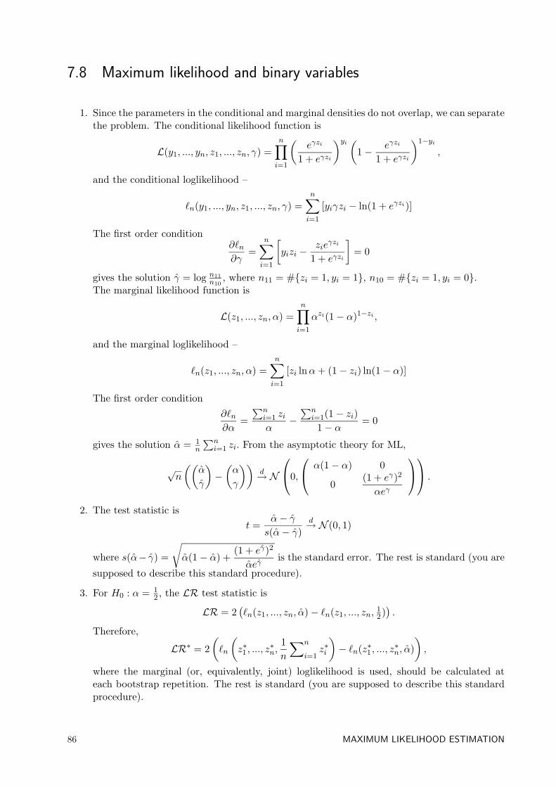
7.8 Maximum likelihood and binary variables
1. Since the parameters in the conditional and marginal densities do not overlap, we can separatethe problem. The conditional likelihood function is
L(y1, ..., yn, z1, ..., zn, γ) =n∏i=1
(eγzi
1 + eγzi
)yi (1− eγzi
1 + eγzi
)1−yi,
and the conditional loglikelihood –
`n(y1, ..., yn, z1, ..., zn, γ) =n∑i=1
[yiγzi − ln(1 + eγzi)]
The first order condition∂`n∂γ
=n∑i=1
[yizi −
zieγzi
1 + eγzi
]= 0
gives the solution γ = log n11n10, where n11 = #zi = 1, yi = 1, n10 = #zi = 1, yi = 0.
The marginal likelihood function is
L(z1, ..., zn, α) =n∏i=1
αzi(1− α)1−zi ,
and the marginal loglikelihood –
`n(z1, ..., zn, α) =n∑i=1
[zi lnα+ (1− zi) ln(1− α)]
The first order condition∂`n∂α
=∑n
i=1 ziα
−∑n
i=1(1− zi)1− α
= 0
gives the solution α = 1n
∑ni=1 zi. From the asymptotic theory for ML,
√n
((α
γ
)−(α
γ
))d→ N
0,
α(1− α) 0
0(1 + eγ)2
αeγ
.
2. The test statistic ist =
α− γs(α− γ)
d→ N (0, 1)
where s(α− γ) =
√α(1− α) +
(1 + eγ)2
αeγis the standard error. The rest is standard (you are
supposed to describe this standard procedure).
3. For H0 : α = 12 , the LR test statistic is
LR = 2(`n(z1, ..., zn, α)− `n(z1, ..., zn,
12)).
Therefore,
LR∗ = 2(`n
(z∗1 , ..., z
∗n,
1n
∑n
i=1z∗i
)− `n(z∗1 , ..., z
∗n, α)
),
where the marginal (or, equivalently, joint) loglikelihood is used, should be calculated ateach bootstrap repetition. The rest is standard (you are supposed to describe this standardprocedure).
86 MAXIMUM LIKELIHOOD ESTIMATION
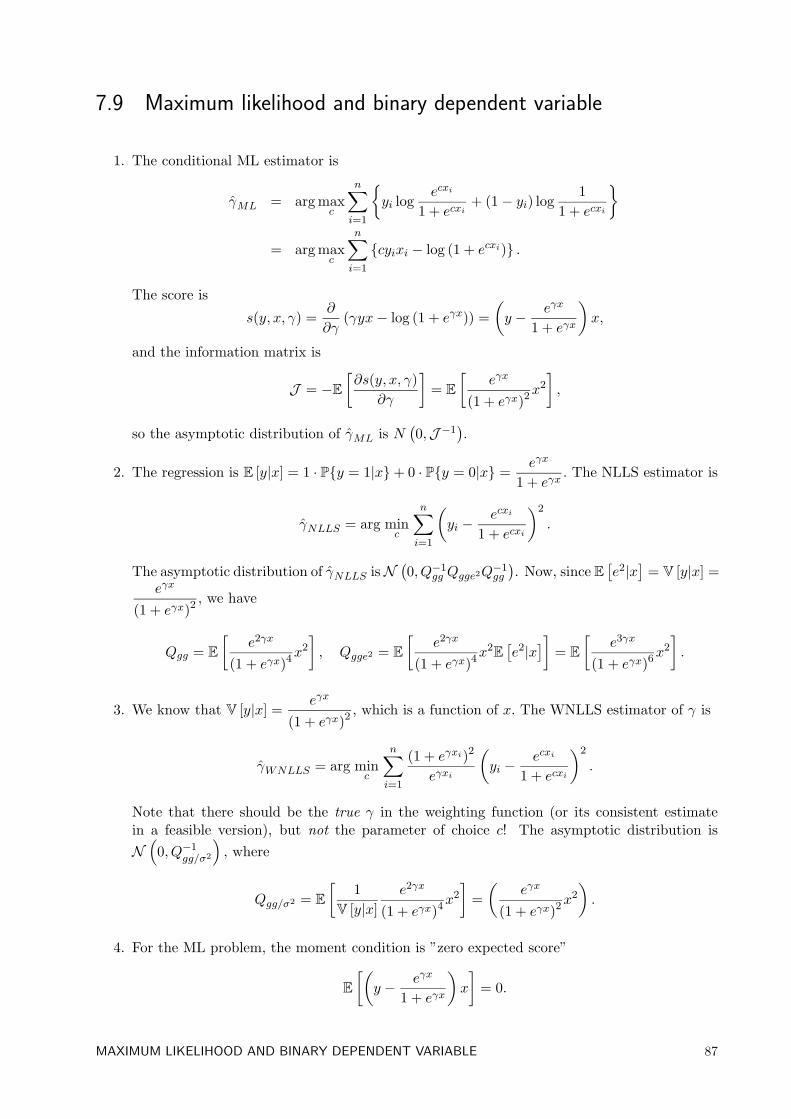
7.9 Maximum likelihood and binary dependent variable
1. The conditional ML estimator is
γML = arg maxc
n∑i=1
yi log
ecxi
1 + ecxi+ (1− yi) log
11 + ecxi
= arg maxc
n∑i=1
cyixi − log (1 + ecxi) .
The score is
s(y, x, γ) =∂
∂γ(γyx− log (1 + eγx)) =
(y − eγx
1 + eγx
)x,
and the information matrix is
J = −E[∂s(y, x, γ)
∂γ
]= E
[eγx
(1 + eγx)2x2
],
so the asymptotic distribution of γML is N(0,J −1
).
2. The regression is E [y|x] = 1 · Py = 1|x+ 0 · Py = 0|x =eγx
1 + eγx. The NLLS estimator is
γNLLS = arg minc
n∑i=1
(yi −
ecxi
1 + ecxi
)2
.
The asymptotic distribution of γNLLS isN(0, Q−1
gg Qgge2Q−1gg
). Now, since E
[e2|x
]= V [y|x] =
eγx
(1 + eγx)2 , we have
Qgg = E
[e2γx
(1 + eγx)4x2
], Qgge2 = E
[e2γx
(1 + eγx)4x2E
[e2|x
]]= E
[e3γx
(1 + eγx)6x2
].
3. We know that V [y|x] =eγx
(1 + eγx)2 , which is a function of x. The WNLLS estimator of γ is
γWNLLS = arg minc
n∑i=1
(1 + eγxi)2
eγxi
(yi −
ecxi
1 + ecxi
)2
.
Note that there should be the true γ in the weighting function (or its consistent estimatein a feasible version), but not the parameter of choice c! The asymptotic distribution isN(
0, Q−1gg/σ2
), where
Qgg/σ2 = E
[1
V [y|x]e2γx
(1 + eγx)4x2
]=(
eγx
(1 + eγx)2x2
).
4. For the ML problem, the moment condition is ”zero expected score”
E
[(y − eγx
1 + eγx
)x
]= 0.
MAXIMUM LIKELIHOOD AND BINARY DEPENDENT VARIABLE 87
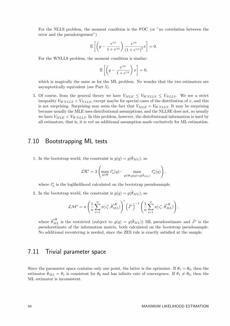
For the NLLS problem, the moment condition is the FOC (or ”no correlation between theerror and the pseudoregressor”)
E
[(y − eγx
1 + eγx
)eγx
(1 + eγx)2x
]= 0.
For the WNLLS problem, the moment condition is similar:
E
[(y − eγx
1 + eγx
)x
]= 0,
which is magically the same as for the ML problem. No wonder that the two estimators areasymptotically equivalent (see Part 5).
5. Of course, from the general theory we have VMLE ≤ VWNLLS ≤ VNLLS . We see a strictinequality VWNLLS < VNLLS , except maybe for special cases of the distribution of x, and thisis not surprising. Surprising may seem the fact that VMLE = VWNLLS . It may be surprisingbecause usually the MLE uses distributional assumptions, and the NLLSE does not, so usuallywe have VMLE < VWNLLS . In this problem, however, the distributional information is used byall estimators, that is, it is not an additional assumption made exclusively for ML estimation.
7.10 Bootstrapping ML tests
1. In the bootstrap world, the constraint is g(q) = g(θML), so
LR∗ = 2
(maxq∈Θ
`∗n(q)− maxq∈Θ,g(q)=g(θML)
`∗n(q)
),
where `∗n is the loglikelihood calculated on the bootstrap pseudosample.
2. In the bootstrap world, the constraint is g(q) = g(θML), so
LM∗ = n
(1n
n∑i=1
s(z∗i , θ∗RML)
)′ (J∗)−1
(1n
n∑i=1
s(z∗i , θ∗RML)
),
where θ∗RML is the restricted (subject to g(q) = g(θML)) ML pseudoestimate and J∗ is the
pseudoestimate of the information matrix, both calculated on the bootstrap pseudosample.No additional recentering is needed, since the ZES rule is exactly satisfied at the sample.
7.11 Trivial parameter space
Since the parameter space contains only one point, the latter is the optimizer. If θ1 = θ0, then theestimator θML = θ1 is consistent for θ0 and has infinite rate of convergence. If θ1 6= θ0, then theML estimator is inconsistent.
88 MAXIMUM LIKELIHOOD ESTIMATION
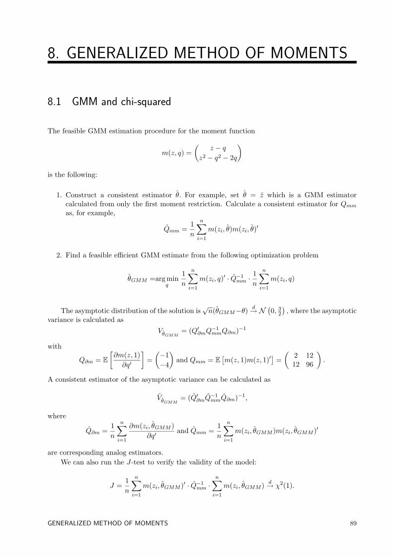
8. GENERALIZED METHOD OF MOMENTS
8.1 GMM and chi-squared
The feasible GMM estimation procedure for the moment function
m(z, q) =(
z − qz2 − q2 − 2q
)is the following:
1. Construct a consistent estimator θ. For example, set θ = z which is a GMM estimatorcalculated from only the first moment restriction. Calculate a consistent estimator for Qmmas, for example,
Qmm =1n
n∑i=1
m(zi, θ)m(zi, θ)′
2. Find a feasible efficient GMM estimate from the following optimization problem
θGMM =arg minq
1n
n∑i=1
m(zi, q)′ · Q−1mm ·
1n
n∑i=1
m(zi, q)
The asymptotic distribution of the solution is√n(θGMM−θ)
d→ N(0, 3
2
), where the asymptotic
variance is calculated as
VθGMM= (Q′∂mQ
−1mmQ∂m)−1
with
Q∂m = E
[∂m(z, 1)∂q′
]=(−1−4
)and Qmm = E
[m(z, 1)m(z, 1)′
]=(
2 1212 96
).
A consistent estimator of the asymptotic variance can be calculated as
VθGMM= (Q′∂mQ
−1mmQ∂m)−1,
where
Q∂m =1n
n∑i=1
∂m(zi, θGMM )∂q′
and Qmm =1n
n∑i=1
m(zi, θGMM )m(zi, θGMM )′
are corresponding analog estimators.We can also run the J-test to verify the validity of the model:
J =1n
n∑i=1
m(zi, θGMM )′ · Q−1mm ·
n∑i=1
m(zi, θGMM ) d→ χ2(1).
GENERALIZED METHOD OF MOMENTS 89
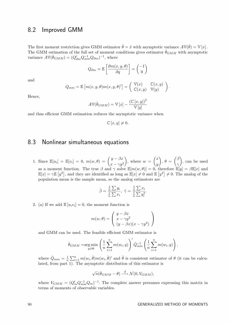
8.2 Improved GMM
The first moment restriction gives GMM estimator θ = x with asymptotic variance AV(θ) = V [x] .The GMM estimation of the full set of moment conditions gives estimator θGMM with asymptoticvariance AV(θGMM ) = (Q′∂mQ
−1mmQ∂m)−1, where
Q∂m = E
[∂m(x, y, θ)
∂q
]=(−10
)and
Qmm = E
[m(x, y, θ)m(x, y, θ)′
]=(V(x) C(x, y)C(x, y) V(y)
).
Hence,
AV(θGMM ) = V [x]− (C [x, y])2
V [y]
and thus efficient GMM estimation reduces the asymptotic variance when
C [x, y] 6= 0.
8.3 Nonlinear simultaneous equations
1. Since E[ui] = E[vi] = 0, m(w, θ) =(y − βxx− γy2
), where w =
(x
y
), θ =
(β
γ
), can be used
as a moment function. The true β and γ solve E[m(w, θ)] = 0, therefore E[y] = βE[x] andE[x] = γE
[y2], and they are identified as long as E[x] 6= 0 and E
[y2]6= 0. The analog of the
population mean is the sample mean, so the analog estimators are
β =1n
∑yi
1n
∑xi, γ =
1n
∑xi
1n
∑y2i
.
2. (a) If we add E [uivi] = 0, the moment function is
m(w, θ) =
y − βxx− γy2
(y − βx)(x− γy2)
and GMM can be used. The feasible efficient GMM estimator is
θGMM =arg minq∈Θ
(1n
n∑i=1
m(wi, q)
)′Q−1mm
(1n
n∑i=1
m(wi, q)
),
where Qmm = 1n
∑ni=1m(wi, θ)m(wi, θ)′ and θ is consistent estimator of θ (it can be calcu-
lated, from part 1). The asymptotic distribution of this estimator is
√n(θGMM − θ)
d−→ N (0, VGMM ),
where VGMM = (Q′mQ−1mmQm)−1. The complete answer presumes expressing this matrix in
terms of moments of observable variables.
90 GENERALIZED METHOD OF MOMENTS
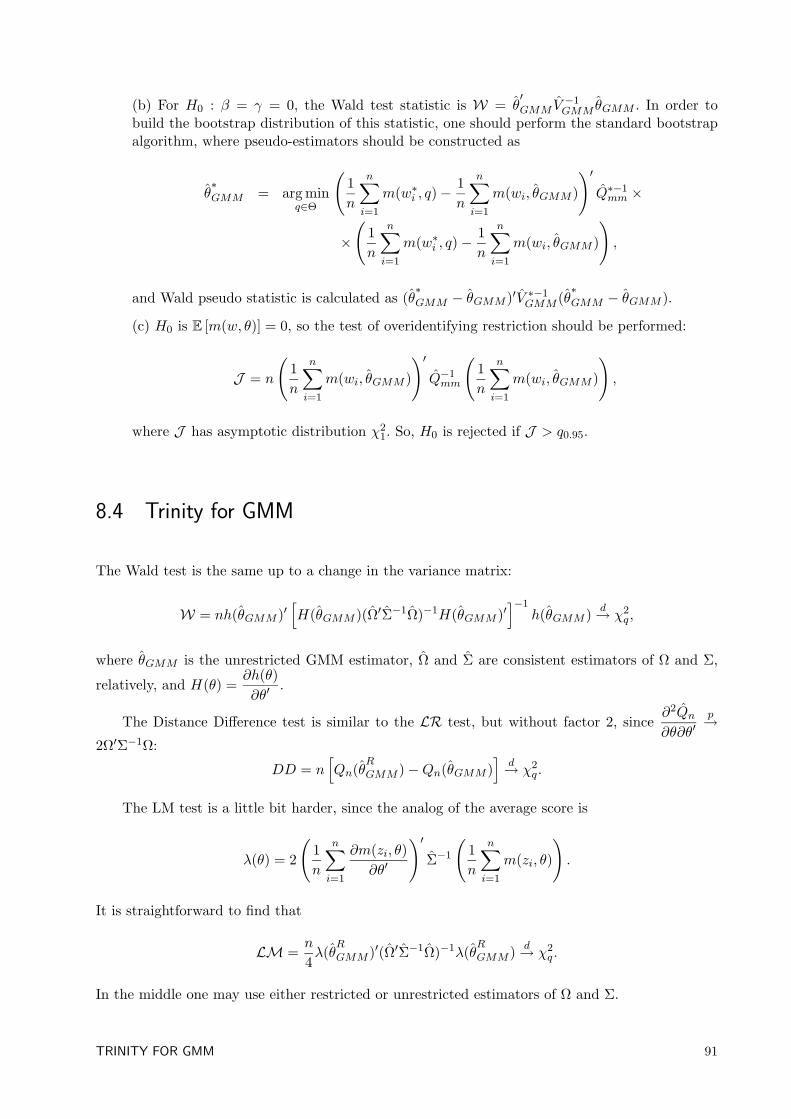
(b) For H0 : β = γ = 0, the Wald test statistic is W = θ′GMM V
−1GMM θGMM . In order to
build the bootstrap distribution of this statistic, one should perform the standard bootstrapalgorithm, where pseudo-estimators should be constructed as
θ∗GMM = arg min
q∈Θ
(1n
n∑i=1
m(w∗i , q)−1n
n∑i=1
m(wi, θGMM )
)′Q∗−1mm ×
×
(1n
n∑i=1
m(w∗i , q)−1n
n∑i=1
m(wi, θGMM )
),
and Wald pseudo statistic is calculated as (θ∗GMM − θGMM )′V ∗−1
GMM (θ∗GMM − θGMM ).
(c) H0 is E [m(w, θ)] = 0, so the test of overidentifying restriction should be performed:
J = n
(1n
n∑i=1
m(wi, θGMM )
)′Q−1mm
(1n
n∑i=1
m(wi, θGMM )
),
where J has asymptotic distribution χ21. So, H0 is rejected if J > q0.95.
8.4 Trinity for GMM
The Wald test is the same up to a change in the variance matrix:
W = nh(θGMM )′[H(θGMM )(Ω′Σ−1Ω)−1H(θGMM )′
]−1h(θGMM ) d→ χ2
q ,
where θGMM is the unrestricted GMM estimator, Ω and Σ are consistent estimators of Ω and Σ,
relatively, and H(θ) =∂h(θ)∂θ′
.
The Distance Difference test is similar to the LR test, but without factor 2, since∂2Qn∂θ∂θ′
p→2Ω′Σ−1Ω:
DD = n[Qn(θ
R
GMM )−Qn(θGMM )]
d→ χ2q .
The LM test is a little bit harder, since the analog of the average score is
λ(θ) = 2
(1n
n∑i=1
∂m(zi, θ)∂θ′
)′Σ−1
(1n
n∑i=1
m(zi, θ)
).
It is straightforward to find that
LM =n
4λ(θ
R
GMM )′(Ω′Σ−1Ω)−1λ(θR
GMM ) d→ χ2q .
In the middle one may use either restricted or unrestricted estimators of Ω and Σ.
TRINITY FOR GMM 91
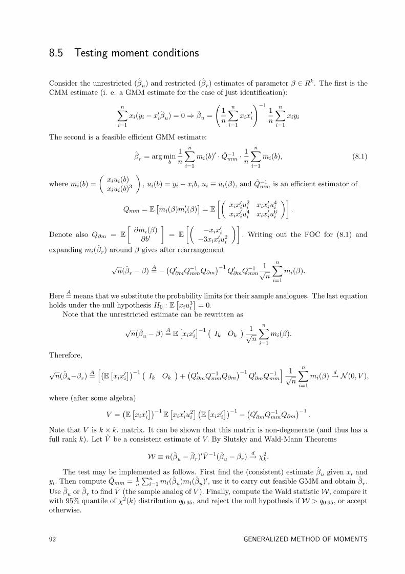
8.5 Testing moment conditions
Consider the unrestricted (βu) and restricted (βr) estimates of parameter β ∈ Rk. The first is theCMM estimate (i. e. a GMM estimate for the case of just identification):
n∑i=1
xi(yi − x′iβu) = 0⇒ βu =
(1n
n∑i=1
xix′i
)−11n
n∑i=1
xiyi
The second is a feasible efficient GMM estimate:
βr = arg minb
1n
n∑i=1
mi(b)′ · Q−1mm ·
1n
n∑i=1
mi(b), (8.1)
where mi(b) =(xiui(b)xiui(b)3
), ui(b) = yi − xib, ui ≡ ui(β), and Q−1
mm is an efficient estimator of
Qmm = E
[mi(β)m′i(β)
]= E
[(xix′iu
2i xix
′iu
4i
xix′iu
4i xix
′iu
6i
)].
Denote also Q∂m = E
[∂mi(β)∂b′
]= E
[(−xix′i−3xix′iu
2i
)]. Writing out the FOC for (8.1) and
expanding mi(βr) around β gives after rearrangement
√n(βr − β) A= −
(Q′∂mQ
−1mmQ∂m
)−1Q′∂mQ
−1mm
1√n
n∑i=1
mi(β).
Here A= means that we substitute the probability limits for their sample analogues. The last equationholds under the null hypothesis H0 : E
[xiu
3i
]= 0.
Note that the unrestricted estimate can be rewritten as
√n(βu − β) A= E
[xix′i
]−1 (Ik Ok
) 1√n
n∑i=1
mi(β).
Therefore,
√n(βu−βr)
A=[(E
[xix′i
])−1 (Ik Ok
)+(Q′∂mQ
−1mmQ∂m
)−1Q′∂mQ
−1mm
] 1√n
n∑i=1
mi(β) d→ N (0, V ),
where (after some algebra)
V =(E
[xix′i
])−1E
[xix′iu
2i
] (E
[xix′i
])−1 −(Q′∂mQ
−1mmQ∂m
)−1.
Note that V is k × k. matrix. It can be shown that this matrix is non-degenerate (and thus has afull rank k). Let V be a consistent estimate of V. By Slutsky and Wald-Mann Theorems
W ≡ n(βu − βr)′V −1(βu − βr)d→ χ2
k.
The test may be implemented as follows. First find the (consistent) estimate βu given xi andyi. Then compute Qmm = 1
n
∑ni=1mi(βu)mi(βu)′, use it to carry out feasible GMM and obtain βr.
Use βu or βr to find V (the sample analog of V ). Finally, compute the Wald statisticW, compare itwith 95% quantile of χ2(k) distribution q0.95, and reject the null hypothesis if W > q0.95, or acceptotherwise.
92 GENERALIZED METHOD OF MOMENTS
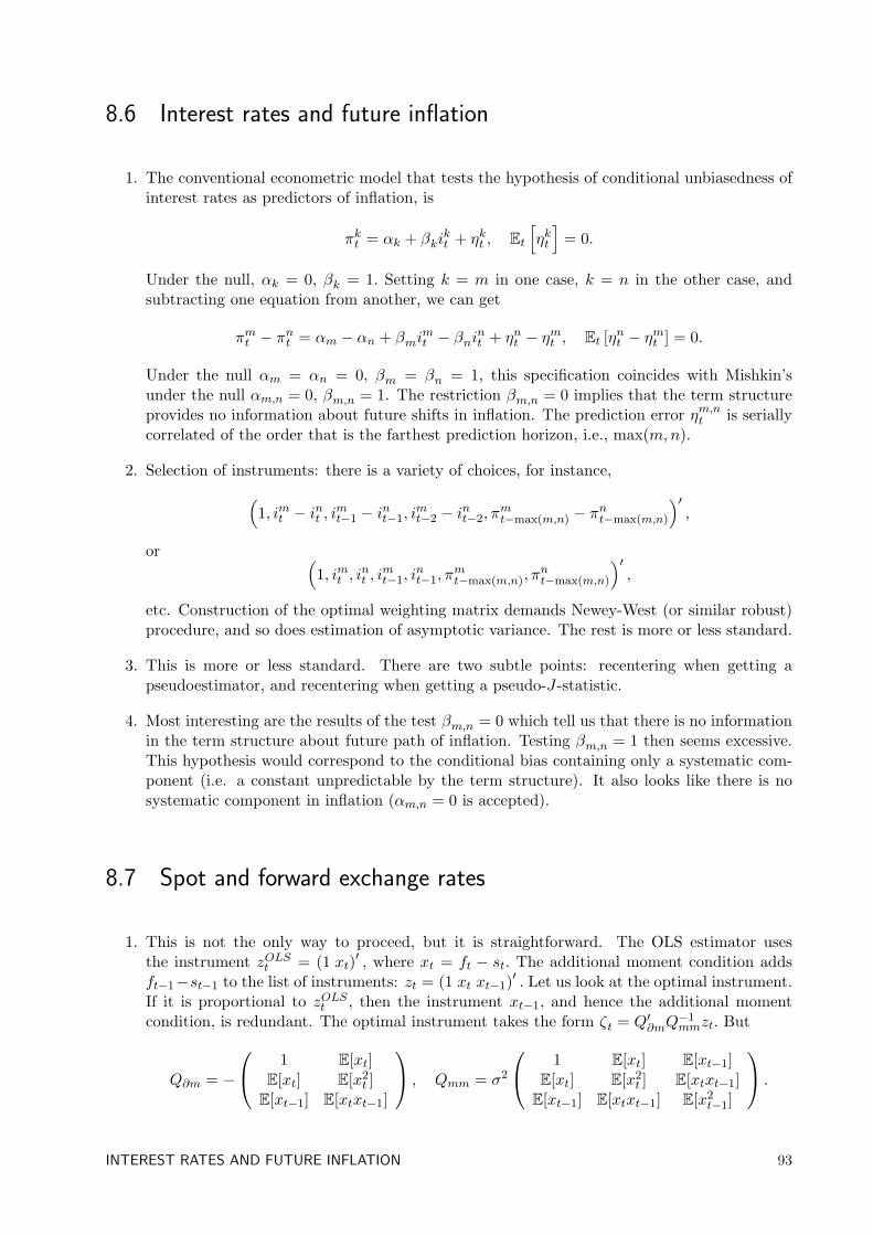
8.6 Interest rates and future inflation
1. The conventional econometric model that tests the hypothesis of conditional unbiasedness ofinterest rates as predictors of inflation, is
πkt = αk + βkikt + ηkt , Et
[ηkt
]= 0.
Under the null, αk = 0, βk = 1. Setting k = m in one case, k = n in the other case, andsubtracting one equation from another, we can get
πmt − πnt = αm − αn + βmimt − βnint + ηnt − ηmt , Et [ηnt − ηmt ] = 0.
Under the null αm = αn = 0, βm = βn = 1, this specification coincides with Mishkin’sunder the null αm,n = 0, βm,n = 1. The restriction βm,n = 0 implies that the term structureprovides no information about future shifts in inflation. The prediction error ηm,nt is seriallycorrelated of the order that is the farthest prediction horizon, i.e., max(m,n).
2. Selection of instruments: there is a variety of choices, for instance,(1, imt − int , imt−1 − int−1, i
mt−2 − int−2, π
mt−max(m,n) − π
nt−max(m,n)
)′,
or (1, imt , i
nt , i
mt−1, i
nt−1, π
mt−max(m,n), π
nt−max(m,n)
)′,
etc. Construction of the optimal weighting matrix demands Newey-West (or similar robust)procedure, and so does estimation of asymptotic variance. The rest is more or less standard.
3. This is more or less standard. There are two subtle points: recentering when getting apseudoestimator, and recentering when getting a pseudo-J-statistic.
4. Most interesting are the results of the test βm,n = 0 which tell us that there is no informationin the term structure about future path of inflation. Testing βm,n = 1 then seems excessive.This hypothesis would correspond to the conditional bias containing only a systematic com-ponent (i.e. a constant unpredictable by the term structure). It also looks like there is nosystematic component in inflation (αm,n = 0 is accepted).
8.7 Spot and forward exchange rates
1. This is not the only way to proceed, but it is straightforward. The OLS estimator usesthe instrument zOLSt = (1 xt)
′ , where xt = ft − st. The additional moment condition addsft−1−st−1 to the list of instruments: zt = (1 xt xt−1)′ . Let us look at the optimal instrument.If it is proportional to zOLSt , then the instrument xt−1, and hence the additional momentcondition, is redundant. The optimal instrument takes the form ζt = Q′∂mQ
−1mmzt. But
Q∂m = −
1 E[xt]E[xt] E[x2
t ]E[xt−1] E[xtxt−1]
, Qmm = σ2
1 E[xt] E[xt−1]E[xt] E[x2
t ] E[xtxt−1]E[xt−1] E[xtxt−1] E[x2
t−1]
.
INTEREST RATES AND FUTURE INFLATION 93
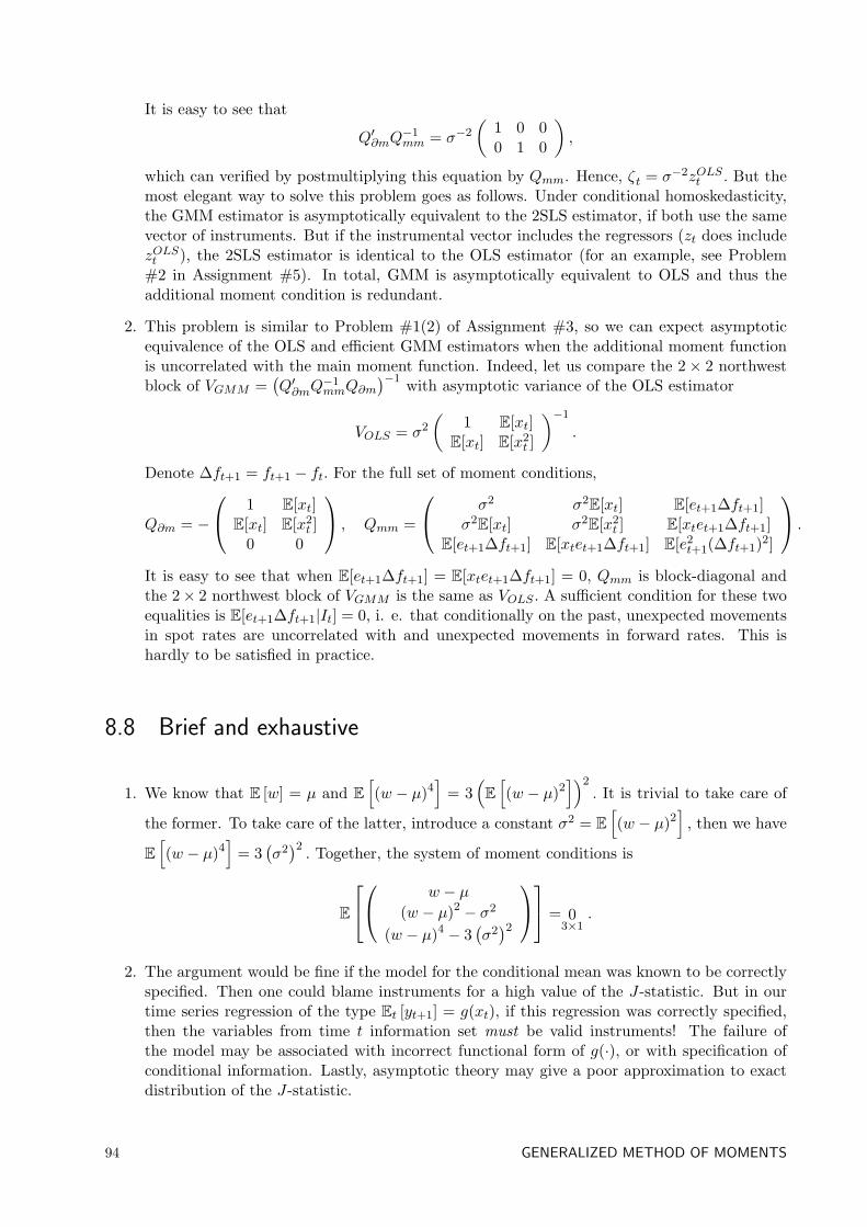
It is easy to see that
Q′∂mQ−1mm = σ−2
(1 0 00 1 0
),
which can verified by postmultiplying this equation by Qmm. Hence, ζt = σ−2zOLSt . But themost elegant way to solve this problem goes as follows. Under conditional homoskedasticity,the GMM estimator is asymptotically equivalent to the 2SLS estimator, if both use the samevector of instruments. But if the instrumental vector includes the regressors (zt does includezOLSt ), the 2SLS estimator is identical to the OLS estimator (for an example, see Problem#2 in Assignment #5). In total, GMM is asymptotically equivalent to OLS and thus theadditional moment condition is redundant.
2. This problem is similar to Problem #1(2) of Assignment #3, so we can expect asymptoticequivalence of the OLS and efficient GMM estimators when the additional moment functionis uncorrelated with the main moment function. Indeed, let us compare the 2× 2 northwestblock of VGMM =
(Q′∂mQ
−1mmQ∂m
)−1 with asymptotic variance of the OLS estimator
VOLS = σ2
(1 E[xt]
E[xt] E[x2t ]
)−1
.
Denote ∆ft+1 = ft+1 − ft. For the full set of moment conditions,
Q∂m = −
1 E[xt]E[xt] E[x2
t ]0 0
, Qmm =
σ2 σ2E[xt] E[et+1∆ft+1]
σ2E[xt] σ2
E[x2t ] E[xtet+1∆ft+1]
E[et+1∆ft+1] E[xtet+1∆ft+1] E[e2t+1(∆ft+1)2]
.
It is easy to see that when E[et+1∆ft+1] = E[xtet+1∆ft+1] = 0, Qmm is block-diagonal andthe 2× 2 northwest block of VGMM is the same as VOLS . A sufficient condition for these twoequalities is E[et+1∆ft+1|It] = 0, i. e. that conditionally on the past, unexpected movementsin spot rates are uncorrelated with and unexpected movements in forward rates. This ishardly to be satisfied in practice.
8.8 Brief and exhaustive
1. We know that E [w] = µ and E[(w − µ)4
]= 3
(E
[(w − µ)2
])2. It is trivial to take care of
the former. To take care of the latter, introduce a constant σ2 = E
[(w − µ)2
], then we have
E
[(w − µ)4
]= 3
(σ2)2. Together, the system of moment conditions is
E
w − µ(w − µ)2 − σ2
(w − µ)4 − 3(σ2)2 = 0
3×1.
2. The argument would be fine if the model for the conditional mean was known to be correctlyspecified. Then one could blame instruments for a high value of the J-statistic. But in ourtime series regression of the type Et [yt+1] = g(xt), if this regression was correctly specified,then the variables from time t information set must be valid instruments! The failure ofthe model may be associated with incorrect functional form of g(·), or with specification ofconditional information. Lastly, asymptotic theory may give a poor approximation to exactdistribution of the J-statistic.
94 GENERALIZED METHOD OF MOMENTS
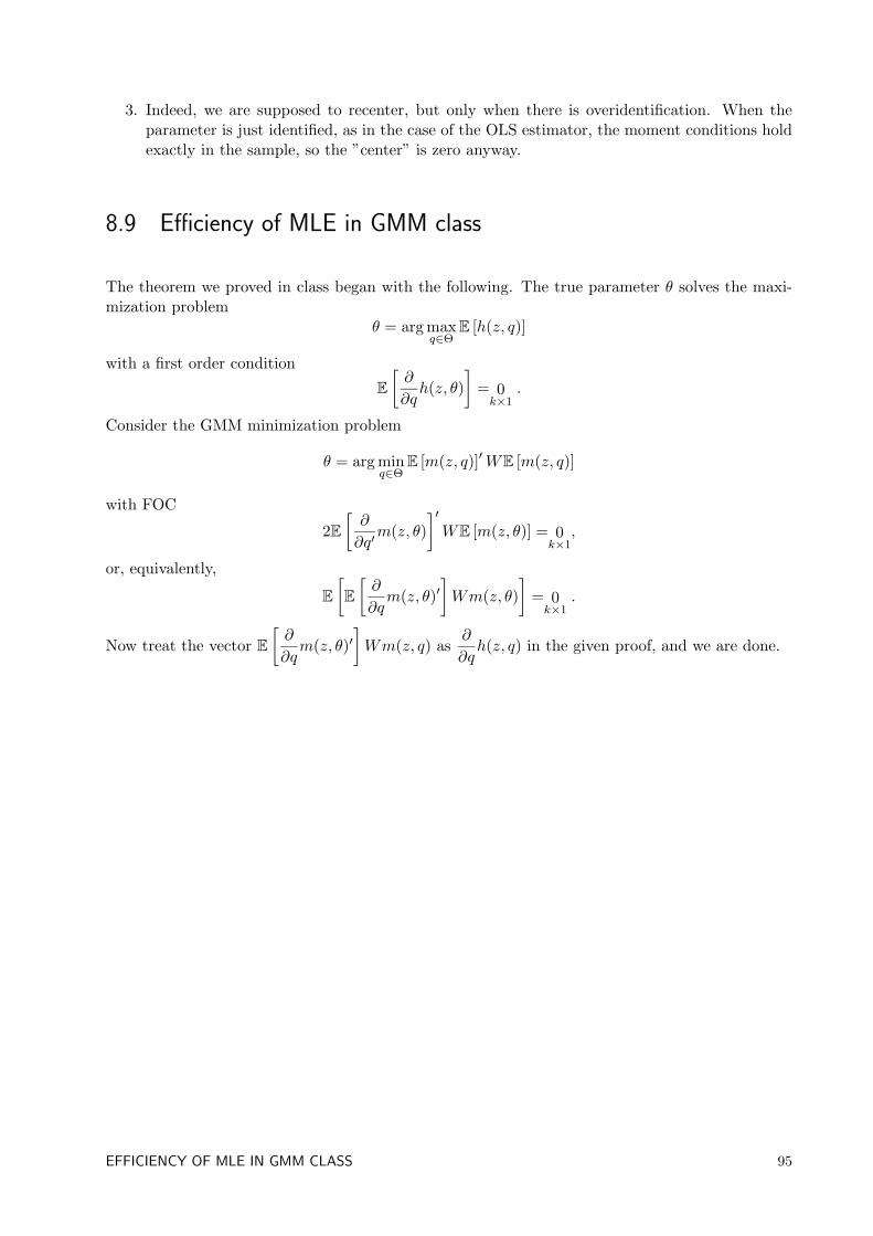
3. Indeed, we are supposed to recenter, but only when there is overidentification. When theparameter is just identified, as in the case of the OLS estimator, the moment conditions holdexactly in the sample, so the ”center” is zero anyway.
8.9 Efficiency of MLE in GMM class
The theorem we proved in class began with the following. The true parameter θ solves the maxi-mization problem
θ = arg maxq∈Θ
E [h(z, q)]
with a first order condition
E
[∂
∂qh(z, θ)
]= 0k×1
.
Consider the GMM minimization problem
θ = arg minq∈Θ
E [m(z, q)]′WE [m(z, q)]
with FOC
2E[∂
∂q′m(z, θ)
]′WE [m(z, θ)] = 0
k×1,
or, equivalently,
E
[E
[∂
∂qm(z, θ)′
]Wm(z, θ)
]= 0k×1
.
Now treat the vector E[∂
∂qm(z, θ)′
]Wm(z, q) as
∂
∂qh(z, q) in the given proof, and we are done.
EFFICIENCY OF MLE IN GMM CLASS 95

96 GENERALIZED METHOD OF MOMENTS
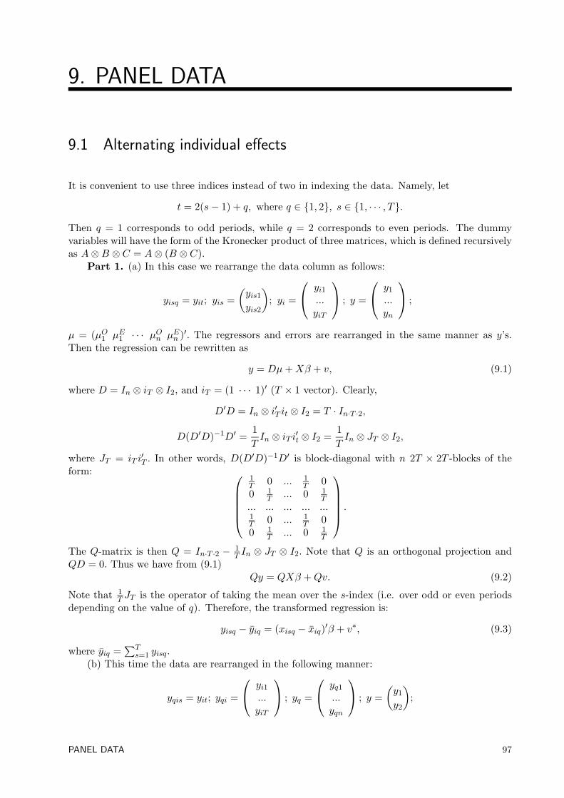
9. PANEL DATA
9.1 Alternating individual effects
It is convenient to use three indices instead of two in indexing the data. Namely, let
t = 2(s− 1) + q, where q ∈ 1, 2, s ∈ 1, · · · , T.
Then q = 1 corresponds to odd periods, while q = 2 corresponds to even periods. The dummyvariables will have the form of the Kronecker product of three matrices, which is defined recursivelyas A⊗B ⊗ C = A⊗ (B ⊗ C).
Part 1. (a) In this case we rearrange the data column as follows:
yisq = yit; yis =(yis1yis2
); yi =
yi1...yiT
; y =
y1
...yn
;
µ = (µO1 µE1 · · · µOn µEn )′. The regressors and errors are rearranged in the same manner as y’s.Then the regression can be rewritten as
y = Dµ+Xβ + v, (9.1)
where D = In ⊗ iT ⊗ I2, and iT = (1 · · · 1)′ (T × 1 vector). Clearly,
D′D = In ⊗ i′T it ⊗ I2 = T · In·T ·2,
D(D′D)−1D′ =1TIn ⊗ iT i′t ⊗ I2 =
1TIn ⊗ JT ⊗ I2,
where JT = iT i′T . In other words, D(D′D)−1D′ is block-diagonal with n 2T × 2T -blocks of the
form: 1T 0 ... 1
T 00 1
T ... 0 1T
... ... ... ... ...1T 0 ... 1
T 00 1
T ... 0 1T
.
The Q-matrix is then Q = In·T ·2 − 1T In ⊗ JT ⊗ I2. Note that Q is an orthogonal projection and
QD = 0. Thus we have from (9.1)Qy = QXβ +Qv. (9.2)
Note that 1T JT is the operator of taking the mean over the s-index (i.e. over odd or even periods
depending on the value of q). Therefore, the transformed regression is:
yisq − yiq = (xisq − xiq)′β + v∗, (9.3)
where yiq =∑T
s=1 yisq.(b) This time the data are rearranged in the following manner:
yqis = yit; yqi =
yi1...yiT
; yq =
yq1...yqn
; y =(y1
y2
);
PANEL DATA 97
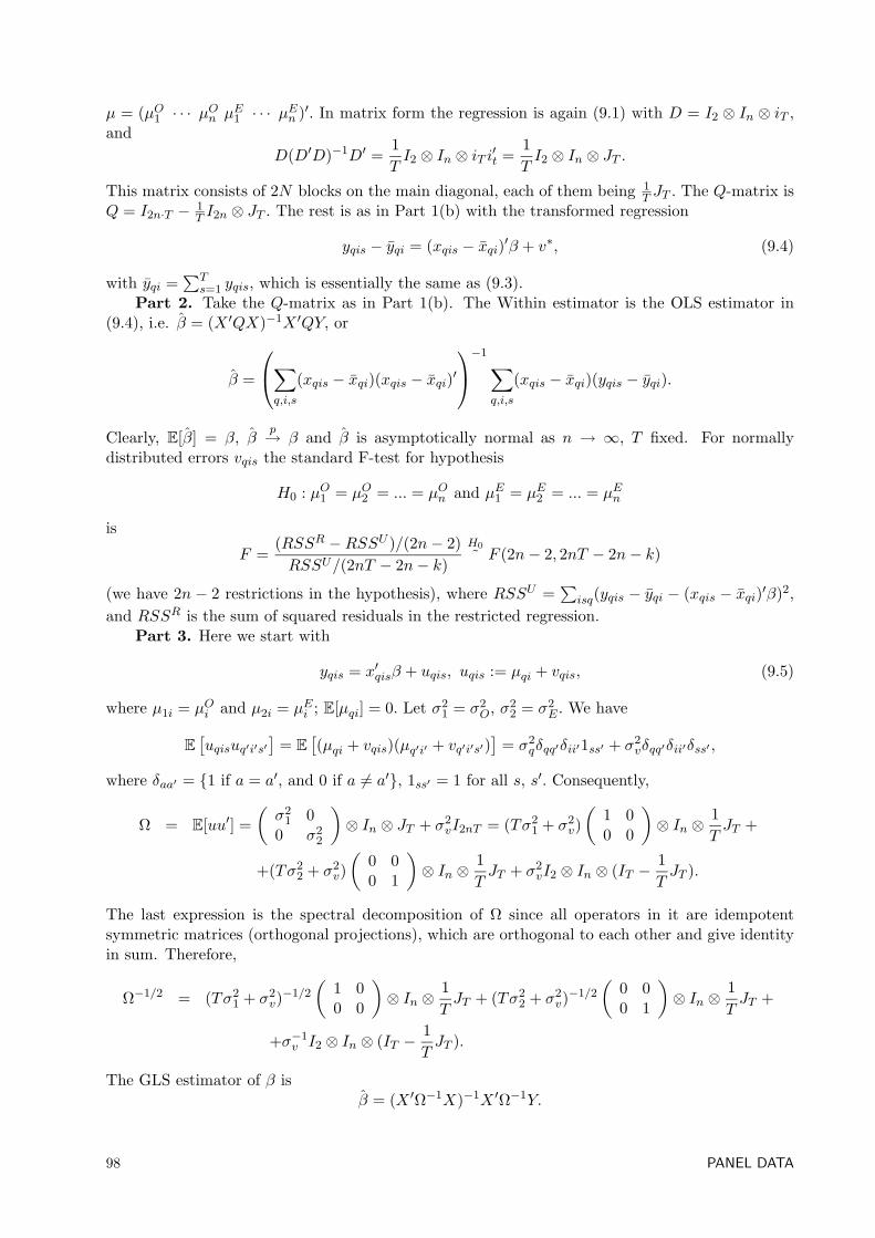
µ = (µO1 · · · µOn µE1 · · · µEn )′. In matrix form the regression is again (9.1) with D = I2 ⊗ In ⊗ iT ,and
D(D′D)−1D′ =1TI2 ⊗ In ⊗ iT i′t =
1TI2 ⊗ In ⊗ JT .
This matrix consists of 2N blocks on the main diagonal, each of them being 1T JT . The Q-matrix is
Q = I2n·T − 1T I2n ⊗ JT . The rest is as in Part 1(b) with the transformed regression
yqis − yqi = (xqis − xqi)′β + v∗, (9.4)
with yqi =∑T
s=1 yqis, which is essentially the same as (9.3).Part 2. Take the Q-matrix as in Part 1(b). The Within estimator is the OLS estimator in
(9.4), i.e. β = (X ′QX)−1X ′QY, or
β =
∑q,i,s
(xqis − xqi)(xqis − xqi)′−1∑
q,i,s
(xqis − xqi)(yqis − yqi).
Clearly, E[β] = β, βp→ β and β is asymptotically normal as n → ∞, T fixed. For normally
distributed errors vqis the standard F-test for hypothesis
H0 : µO1 = µO2 = ... = µOn and µE1 = µE2 = ... = µEn
is
F =(RSSR −RSSU )/(2n− 2)RSSU/(2nT − 2n− k)
H0
˜ F (2n− 2, 2nT − 2n− k)
(we have 2n − 2 restrictions in the hypothesis), where RSSU =∑
isq(yqis − yqi − (xqis − xqi)′β)2,
and RSSR is the sum of squared residuals in the restricted regression.Part 3. Here we start with
yqis = x′qisβ + uqis, uqis := µqi + vqis, (9.5)
where µ1i = µOi and µ2i = µEi ; E[µqi] = 0. Let σ21 = σ2
O, σ22 = σ2
E . We have
E
[uqisuq′i′s′
]= E
[(µqi + vqis)(µq′i′ + vq′i′s′)
]= σ2
qδqq′δii′1ss′ + σ2vδqq′δii′δss′ ,
where δaa′ = 1 if a = a′, and 0 if a 6= a′, 1ss′ = 1 for all s, s′. Consequently,
Ω = E[uu′] =(σ2
1 00 σ2
2
)⊗ In ⊗ JT + σ2
vI2nT = (Tσ21 + σ2
v)(
1 00 0
)⊗ In ⊗
1TJT +
+(Tσ22 + σ2
v)(
0 00 1
)⊗ In ⊗
1TJT + σ2
vI2 ⊗ In ⊗ (IT −1TJT ).
The last expression is the spectral decomposition of Ω since all operators in it are idempotentsymmetric matrices (orthogonal projections), which are orthogonal to each other and give identityin sum. Therefore,
Ω−1/2 = (Tσ21 + σ2
v)−1/2
(1 00 0
)⊗ In ⊗
1TJT + (Tσ2
2 + σ2v)−1/2
(0 00 1
)⊗ In ⊗
1TJT +
+σ−1v I2 ⊗ In ⊗ (IT −
1TJT ).
The GLS estimator of β isβ = (X ′Ω−1X)−1X ′Ω−1Y.
98 PANEL DATA
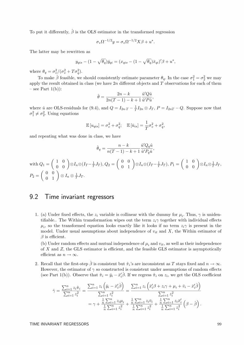
To put it differently, β is the OLS estimator in the transformed regression
σvΩ−1/2y = σvΩ−1/2Xβ + u∗.
The latter may be rewritten as
yqis − (1−√θq)yqi = (xqis − (1−
√θq)xqi)′β + u∗,
where θq = σ2v/(σ
2v + Tσ2
q).To make β feasible, we should consistently estimate parameter θq. In the case σ2
1 = σ22 we may
apply the result obtained in class (we have 2n different objects and T observations for each of them– see Part 1(b)):
θ =2n− k
2n(T − 1)− k + 1u′Qu
u′Pu,
where u are OLS-residuals for (9.4), and Q = I2n·T − 1T I2n ⊗ JT , P = I2nT −Q. Suppose now that
σ21 6= σ2
2. Using equations
E [uqis] = σ2v + σ2
q ; E [uis] =1Tσ2v + σ2
q ,
and repeating what was done in class, we have
θq =n− k
n(T − 1)− k + 1u′Qqu
u′Pqu,
with Q1 =(
1 00 0
)⊗In⊗(IT− 1
T JT ), Q2 =(
0 00 1
)⊗In⊗(IT− 1
T JT ), P1 =(
1 00 0
)⊗In⊗ 1
T JT ,
P2 =(
0 00 1
)⊗ In ⊗ 1
T JT .
9.2 Time invariant regressors
1. (a) Under fixed effects, the zi variable is collinear with the dummy for µi. Thus, γ is uniden-tifiable.. The Within transformation wipes out the term ziγ together with individual effectsµi, so the transformed equation looks exactly like it looks if no term ziγ is present in themodel. Under usual assumptions about independence of vit and X, the Within estimator ofβ is efficient.(b) Under random effects and mutual independence of µi and vit, as well as their independenceof X and Z, the GLS estimator is efficient, and the feasible GLS estimator is asymptoticallyefficient as n→∞.
2. Recall that the first-step β is consistent but πi’s are inconsistent as T stays fixed and n→∞.However, the estimator of γ so constructed is consistent under assumptions of random effects(see Part 1(b)). Observe that πi = yi− x′iβ. If we regress πi on zi, we get the OLS coefficient
γ =∑n
i=1 ziπi∑ni=1 z
2i
=
∑ni=1 zi
(yi − x′iβ
)∑n
i=1 z2i
=
∑ni=1 zi
(x′iβ + ziγ + µi + vi − x′iβ
)∑n
i=1 z2i
= γ +1n
∑ni=1 ziµi
1n
∑ni=1 z
2i
+1n
∑ni=1 zivi
1n
∑ni=1 z
2i
+1n
∑ni=1 zix
′i
1n
∑ni=1 z
2i
(β − β
).
TIME INVARIANT REGRESSORS 99
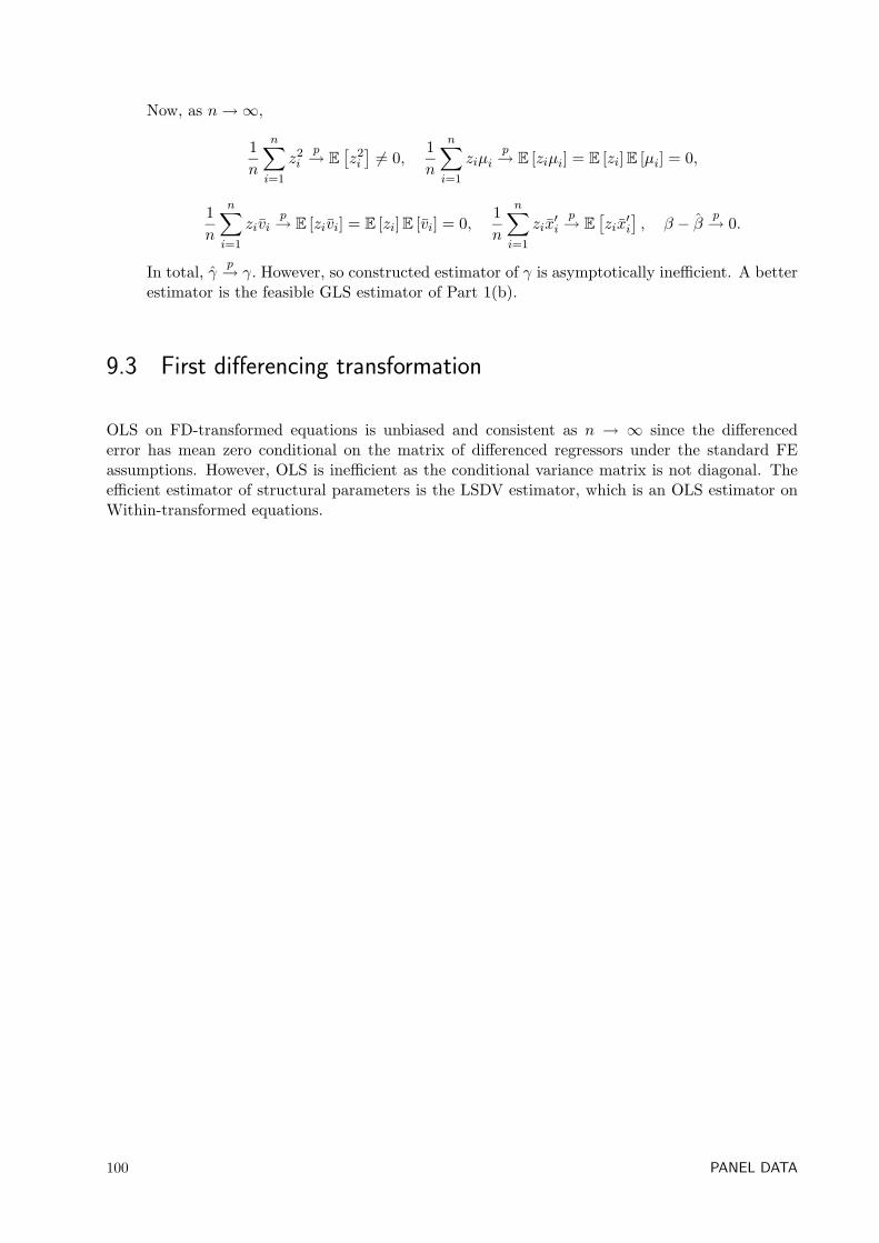
Now, as n→∞,
1n
n∑i=1
z2i
p→ E
[z2i
]6= 0,
1n
n∑i=1
ziµip→ E [ziµi] = E [zi]E [µi] = 0,
1n
n∑i=1
zivip→ E [zivi] = E [zi]E [vi] = 0,
1n
n∑i=1
zix′ip→ E
[zix′i
], β − β p→ 0.
In total, γp→ γ. However, so constructed estimator of γ is asymptotically inefficient. A better
estimator is the feasible GLS estimator of Part 1(b).
9.3 First differencing transformation
OLS on FD-transformed equations is unbiased and consistent as n → ∞ since the differencederror has mean zero conditional on the matrix of differenced regressors under the standard FEassumptions. However, OLS is inefficient as the conditional variance matrix is not diagonal. Theefficient estimator of structural parameters is the LSDV estimator, which is an OLS estimator onWithin-transformed equations.
100 PANEL DATA
10. NONPARAMETRIC ESTIMATION
10.1 Nonparametric regression with discrete regressor
Fix a(j), j = 1, . . . , k. Observe that
g(a(j)) = E[yi|xi = a(j)] =E(yiI[xi = a(j)])E(I[xi = a(j)])
because of the following equalities:
E
[I
[xi = a(j)
]]= 1 · Pxi = a(j)+ 0 · Pxi 6= a(j) = Pxi = a(j),
E
[yiI[xi = a(j)
]]= E
[yiI[xi = a(j)
]|xi = a(j)
]· Pxi = a(j) = E
[yi|xi = a(j)
]· Pxi = a(j).
According to the analogy principle we can construct g(a(j)) as
g(a(j)) =
∑ni=1 yiI
[xi = a(j)
]∑ni=1 I
[xi = a(j)
] .Now let us find its properties. First, according to the LLN,
g(a(j)) =
∑ni=1 yiI
[xi = a(j)
]∑ni=1 I
[xi = a(j)
] p→E
[yiI[xi = a(j)]
]E
[I[xi = a(j)]
] = g(a(j)).
Second,√n(g(a(j))− g(a(j))
)=√n
∑ni=1
(yi − E
[yi|xi = a(j)
])I
[xi = a(j)
]∑ni=1 I
[xi = a(j)
] .
According to the CLT,
1√n
n∑i=1
(yi − E
[yi|xi = a(j)
])I
[xi = a(j)
] d→ N (0, ω) ,
where
ω = V
[(yi − E
[yi|xi = a(j)
])I
[xi = a(j)
]]= E
[(yi − E
[yi|xi = a(j)
])2 |xi = a(j)
]Pxi = a(j)
= V
[yi|xi = a(j)
]Pxi = a(j).
Thus√n(g(a(j))− g(a(j))
) d→ N
(0,V
[yi|xi = a(j)
]Pxi = a(j)
).
10.2 Nonparametric density estimation
(a) Use the hint that E [I [xi ≤ x]] = F (x) to prove the unbiasedness of estimator:
E
[F (x)
]= E
[1n
n∑i=1
I [xi ≤ x]
]=
1n
n∑i=1
E [I [xi ≤ x]] =1n
n∑i=1
F (x) = F (x).
NONPARAMETRIC ESTIMATION 101
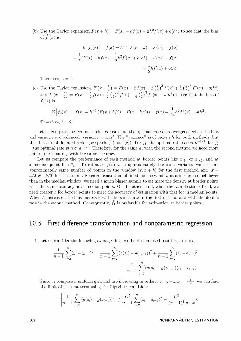
(b) Use the Taylor expansion F (x + h) = F (x) + hf(x) + 12h
2f ′(x) + o(h2) to see that the biasof f1(x) is
E
[f1(x)
]− f(x) = h−1 (F (x+ h)− F (x))− f(x)
=1h
(F (x) + hf(x) +12h2f ′(x) + o(h2)− F (x))− f(x)
=12hf ′(x) + o(h).
Therefore, a = 1.
(c) Use the Taylor expansions F(x+ h
2
)= F (x) + h
2f(x) + 12
(h2
)2f ′(x) + 1
6
(h2
)3f ′′(x) + o(h3)
and F(x− h
2
)= F (x) − h
2f(x) + 12
(h2
)2f ′(x) − 1
6
(h2
)3f ′′(x) + o(h3) to see that the bias of
f2(x) is
E
[f2(x)
]− f(x) = h−1 (F (x+ h/2)− F (x− h/2))− f(x) =
124h2f ′′(x) + o(h2).
Therefore, b = 2.
Let us compare the two methods. We can find the optimal rate of convergence when the biasand variance are balanced: variance ∝ bias2. The ”variance” is of order nh for both methods, butthe ”bias” is of different order (see parts (b) and (c)). For f1, the optimal rate is n ∝ h−1/3, for f2
– the optimal rate is n ∝ h−1/5. Therefore, for the same h, with the second method we need morepoints to estimate f with the same accuracy.
Let us compare the performance of each method at border points like x(1) or x(n), and ata median point like xn. To estimate f(x) with approximately the same variance we need anapproximately same number of points in the window [x, x + h] for the first method and [x −h/2, x+h/2] for the second. Since concentration of points in the window at a border is much lowerthan in the median window, we need a much bigger sample to estimate the density at border pointswith the same accuracy as at median points. On the other hand, when the sample size is fixed, weneed greater h for border points to meet the accuracy of estimation with that for in median points.When h increases, the bias increases with the same rate in the first method and with the doublerate in the second method. Consequently, f1 is preferable for estimation at border points.
10.3 First difference transformation and nonparametric regression
1. Let us consider the following average that can be decomposed into three terms:
1n− 1
n∑i=2
(yi − yi−1)2 =1
n− 1
n∑i=2
(g(zi)− g(zi−1))2 +1
n− 1
n∑i=2
(ei − ei−1)2
+2
n− 1
n∑i=2
(g(zi)− g(zi−1))(ei − ei−1).
Since zi compose a uniform grid and are increasing in order, i.e. zi− zi−1 = 1n−1 , we can find
the limit of the first term using the Lipschitz condition:∣∣∣∣∣ 1n− 1
n∑i=2
(g(zi)− g(zi−1))2
∣∣∣∣∣ ≤ G2
n− 1
n∑i=2
(zi − zi−1)2 =G2
(n− 1)2→
n→∞0
102 NONPARAMETRIC ESTIMATION
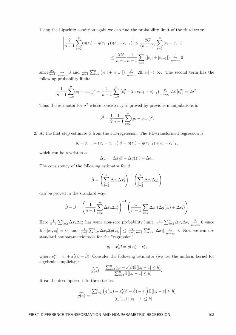
Using the Lipschitz condition again we can find the probability limit of the third term:∣∣∣∣∣ 2n− 1
n∑i=2
(g(zi)− g(zi−1))(ei − ei−1)
∣∣∣∣∣ ≤ 2G(n− 1)2
n∑i=2
|ei − ei−1|
≤ 2Gn− 1
1n− 1
n∑i=2
(|ei|+ |ei−1|)p→
n→∞0
since 2Gn−1 →
n→∞0 and 1
n−1
∑ni=2 (|ei|+ |ei−1|)
p→n→∞
2E |ei| < ∞. The second term has thefollowing probability limit:
1n− 1
n∑i=2
(ei − ei−1)2 =1
n− 1
n∑i=2
(e2i − 2eiei−1 + e2
i−1
) p→n→∞
2E[e2i
]= 2σ2.
Thus the estimator for σ2 whose consistency is proved by previous manipulations is
σ2 =12
1n− 1
n∑i=2
(yi − yi−1)2.
2. At the first step estimate β from the FD-regression. The FD-transformed regression is
yi − yi−1 = (xi − xi−1)′β + g(zi)− g(zi−1) + ei − ei−1,
which can be rewritten as∆yi = ∆x′iβ + ∆g(zi) + ∆ei.
The consistency of the following estimator for β
β =
(n∑i=2
∆xi∆x′i
)−1( n∑i=2
∆xi∆yi
)
can be proved in the standard way:
β − β =
(1
n− 1
n∑i=2
∆xi∆x′i
)−1(1
n− 1
n∑i=2
∆xi(∆g(zi) + ∆ei)
)
Here 1n−1
∑ni=2 ∆xi∆x′i has some non-zero probability limit, 1
n−1
∑ni=2 ∆xi∆ei
p→n→∞
0 since
E[ei|xi, zi] = 0, and∣∣∣ 1n−1
∑ni=2 ∆xi∆g(zi)
∣∣∣ ≤ Gn−1
1n−1
∑ni=2 |∆xi|
p→n→∞
0. Now we can usestandard nonparametric tools for the ”regression”
yi − x′iβ = g(zi) + e∗i ,
where e∗i = ei + x′i(β − β). Consider the following estimator (we use the uniform kernel foralgebraic simplicity):
g(z) =∑n
i=1(yi − x′iβ)I [|zi − z| ≤ h]∑ni=1 I [|zi − z| ≤ h]
.
It can be decomposed into three terms:
g(z) =
∑ni=1
(g(zi) + x′i(β − β) + ei
)I [|zi − z| ≤ h]∑n
i=1 I [|zi − z| ≤ h]
FIRST DIFFERENCE TRANSFORMATION AND NONPARAMETRIC REGRESSION 103
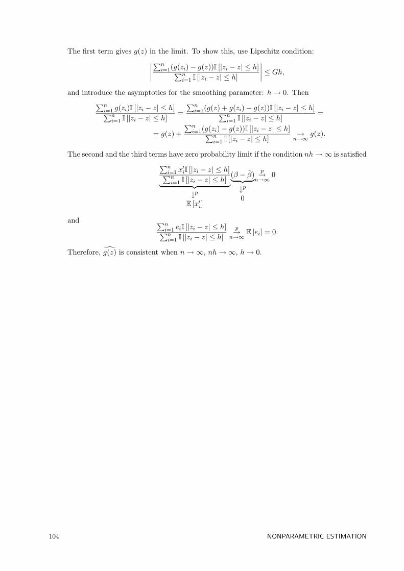
The first term gives g(z) in the limit. To show this, use Lipschitz condition:∣∣∣∣∑ni=1(g(zi)− g(z))I [|zi − z| ≤ h]∑n
i=1 I [|zi − z| ≤ h]
∣∣∣∣ ≤ Gh,and introduce the asymptotics for the smoothing parameter: h→ 0. Then∑n
i=1 g(zi)I [|zi − z| ≤ h]∑ni=1 I [|zi − z| ≤ h]
=∑n
i=1(g(z) + g(zi)− g(z))I [|zi − z| ≤ h]∑ni=1 I [|zi − z| ≤ h]
=
= g(z) +∑n
i=1(g(zi)− g(z))I [|zi − z| ≤ h]∑ni=1 I [|zi − z| ≤ h]
→n→∞
g(z).
The second and the third terms have zero probability limit if the condition nh→∞ is satisfied∑ni=1 x
′iI [|zi − z| ≤ h]∑n
i=1 I [|zi − z| ≤ h]︸ ︷︷ ︸↓pE [x′i]
(β − β)︸ ︷︷ ︸↓p0
p→n→∞
0
and ∑ni=1 eiI [|zi − z| ≤ h]∑ni=1 I [|zi − z| ≤ h]
p→n→∞
E [ei] = 0.
Therefore, g(z) is consistent when n→∞, nh→∞, h→ 0.
104 NONPARAMETRIC ESTIMATION
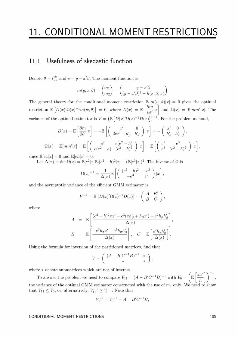
11. CONDITIONAL MOMENT RESTRICTIONS
11.1 Usefulness of skedastic function
Denote θ =(βπ
)and e = y − x′β. The moment function is
m(y, x, θ) =(m1
m2
)=(
y − x′β(y − x′β)2 − h(x, β, π)
)The general theory for the conditional moment restriction E [m(w, θ)|x] = 0 gives the optimal
restriction E[D(x)′Ω(x)−1m(w, θ)
]= 0, where D(x) = E
[∂m
∂θ′|x]
and Ω(x) = E[mm′|x]. The
variance of the optimal estimator is V =(E
[D(x)′Ω(x)−1D(x)
])−1. For the problem at hand,
D(x) = E
[∂m
∂θ′|x]
= −E[(
x′ 02ex′ + h′β h′π
)|x]
= −(
x′ 0h′β h′π
),
Ω(x) = E[mm′|x] = E
[(e2 e(e2 − h)
e(e2 − h) (e2 − h)2
)|x]
= E
[(e2 e3
e3 (e2 − h)2
)|x],
since E[ex|x] = 0 and E[eh|x] = 0.Let ∆(x) ≡ det Ω(x) = E[e2|x]E[(e2 − h)2|x]− (E[e3|x])2. The inverse of Ω is
Ω(x)−1 =1
∆(x)E
[((e2 − h)2 −e3
−e3 e2
)|x],
and the asymptotic variance of the efficient GMM estimator is
V −1 = E
[D(x)′Ω(x)−1D(x)
]=(A B′
B C
),
where
A = E
[(e2 − h)2xx′ − e3(xh′β + hβx
′) + e2hβh′β
∆(x)
],
B = E
[−e3hπx
′ + e2hπh′β
∆(x)
], C = E
[e2hπh
′π
∆(x)
].
Using the formula for inversion of the partitioned matrices, find that
V =(
(A−B′C−1B)−1 ∗∗ ∗
),
where ∗ denote submatrices which are not of interest.
To answer the problem we need to compare V11 = (A−B′C−1B)−1 with V0 =(E
[xx′
h
])−1
,
the variance of the optimal GMM estimator constructed with the use of m1 only. We need to showthat V11 ≤ V0, or, alternatively, V −1
11 ≥ V−1
0 . Note that
V −111 − V
−10 = A−B′C−1B,
CONDITIONAL MOMENT RESTRICTIONS 105
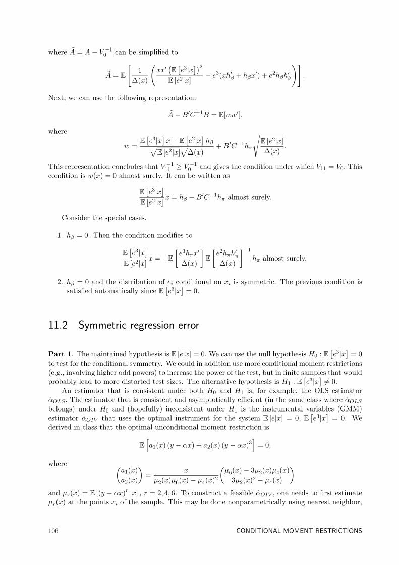
where A = A− V −10 can be simplified to
A = E
[1
∆(x)
(xx′(E
[e3|x
])2E [e2|x]
− e3(xh′β + hβx′) + e2hβh
′β
)].
Next, we can use the following representation:
A−B′C−1B = E[ww′],
where
w =E
[e3|x
]x− E
[e2|x
]hβ√
E [e2|x]√
∆(x)+B′C−1hπ
√E [e2|x]∆(x)
.
This representation concludes that V −111 ≥ V
−10 and gives the condition under which V11 = V0. This
condition is w(x) = 0 almost surely. It can be written as
E
[e3|x
]E [e2|x]
x = hβ −B′C−1hπ almost surely.
Consider the special cases.
1. hβ = 0. Then the condition modifies to
E
[e3|x
]E [e2|x]
x = −E[e3hπx
′
∆(x)
]E
[e2hπh
′π
∆(x)
]−1
hπ almost surely.
2. hβ = 0 and the distribution of ei conditional on xi is symmetric. The previous condition issatisfied automatically since E
[e3|x
]= 0.
11.2 Symmetric regression error
Part 1. The maintained hypothesis is E [e|x] = 0. We can use the null hypothesis H0 : E[e3|x
]= 0
to test for the conditional symmetry. We could in addition use more conditional moment restrictions(e.g., involving higher odd powers) to increase the power of the test, but in finite samples that wouldprobably lead to more distorted test sizes. The alternative hypothesis is H1 : E
[e3|x
]6= 0.
An estimator that is consistent under both H0 and H1 is, for example, the OLS estimatorαOLS . The estimator that is consistent and asymptotically efficient (in the same class where αOLSbelongs) under H0 and (hopefully) inconsistent under H1 is the instrumental variables (GMM)estimator αOIV that uses the optimal instrument for the system E [e|x] = 0, E
[e3|x
]= 0. We
derived in class that the optimal unconditional moment restriction is
E
[a1(x) (y − αx) + a2(x) (y − αx)3
]= 0,
where (a1(x)a2(x)
)=
x
µ2(x)µ6(x)− µ4(x)2
(µ6(x)− 3µ2(x)µ4(x)
3µ2(x)2 − µ4(x)
)and µr(x) = E [(y − αx)r |x] , r = 2, 4, 6. To construct a feasible αOIV , one needs to first estimateµr(x) at the points xi of the sample. This may be done nonparametrically using nearest neighbor,
106 CONDITIONAL MOMENT RESTRICTIONS
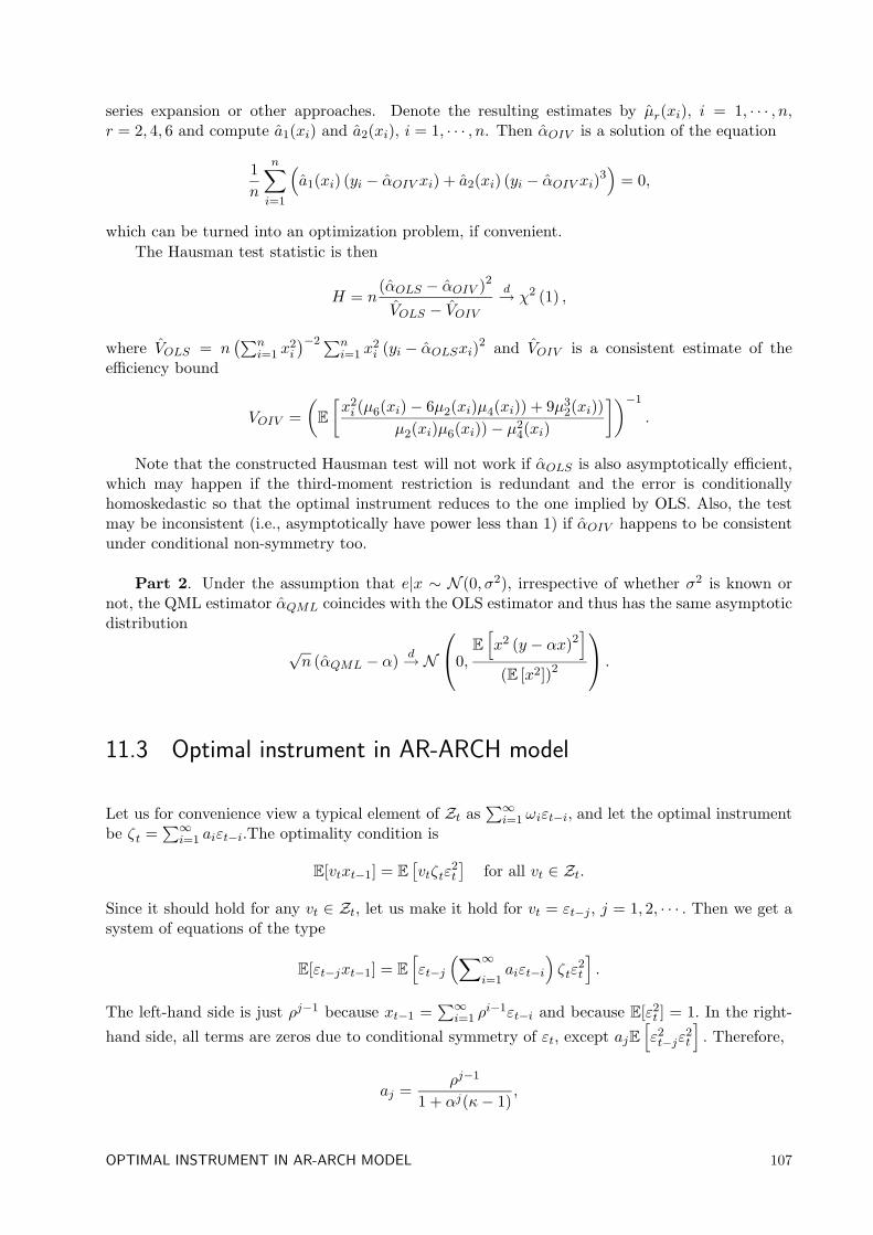
series expansion or other approaches. Denote the resulting estimates by µr(xi), i = 1, · · · , n,r = 2, 4, 6 and compute a1(xi) and a2(xi), i = 1, · · · , n. Then αOIV is a solution of the equation
1n
n∑i=1
(a1(xi) (yi − αOIV xi) + a2(xi) (yi − αOIV xi)3
)= 0,
which can be turned into an optimization problem, if convenient.The Hausman test statistic is then
H = n(αOLS − αOIV )2
VOLS − VOIVd→ χ2 (1) ,
where VOLS = n(∑n
i=1 x2i
)−2∑ni=1 x
2i (yi − αOLSxi)2 and VOIV is a consistent estimate of the
efficiency bound
VOIV =(E
[x2i (µ6(xi)− 6µ2(xi)µ4(xi)) + 9µ3
2(xi))µ2(xi)µ6(xi))− µ2
4(xi)
])−1
.
Note that the constructed Hausman test will not work if αOLS is also asymptotically efficient,which may happen if the third-moment restriction is redundant and the error is conditionallyhomoskedastic so that the optimal instrument reduces to the one implied by OLS. Also, the testmay be inconsistent (i.e., asymptotically have power less than 1) if αOIV happens to be consistentunder conditional non-symmetry too.
Part 2. Under the assumption that e|x ∼ N (0, σ2), irrespective of whether σ2 is known ornot, the QML estimator αQML coincides with the OLS estimator and thus has the same asymptoticdistribution
√n (αQML − α) d→ N
0,E
[x2 (y − αx)2
](E [x2])2
.
11.3 Optimal instrument in AR-ARCH model
Let us for convenience view a typical element of Zt as∑∞
i=1 ωiεt−i, and let the optimal instrumentbe ζt =
∑∞i=1 aiεt−i.The optimality condition is
E[vtxt−1] = E
[vtζtε
2t
]for all vt ∈ Zt.
Since it should hold for any vt ∈ Zt, let us make it hold for vt = εt−j , j = 1, 2, · · · . Then we get asystem of equations of the type
E[εt−jxt−1] = E
[εt−j
(∑∞
i=1aiεt−i
)ζtε
2t
].
The left-hand side is just ρj−1 because xt−1 =∑∞
i=1 ρi−1εt−i and because E[ε2
t ] = 1. In the right-
hand side, all terms are zeros due to conditional symmetry of εt, except ajE[ε2t−jε
2t
]. Therefore,
aj =ρj−1
1 + αj(κ− 1),
OPTIMAL INSTRUMENT IN AR-ARCH MODEL 107
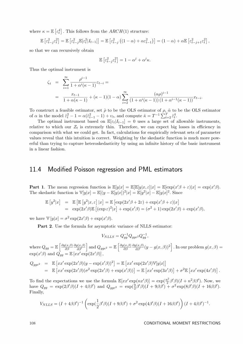
where κ = E
[ε4t
]. This follows from the ARCH(1) structure:
E
[ε2t−jε
2t
]= E
[ε2t−jE[ε2
t |It−1]]
= E
[ε2t−j((1− α) + αε2
t−1
)]= (1− α) + αE
[ε2t−j+1ε
2t
],
so that we can recursively obtain
E
[ε2t−jε
2t
]= 1− αj + αjκ.
Thus the optimal instrument is
ζt =∞∑i=1
ρi−1
1 + αi(κ− 1)εt−i =
=xt−1
1 + α(κ− 1)+ (κ− 1)(1− α)
∞∑i=2
(αρ)i−1
(1 + αi(κ− 1)) (1 + αi−1(κ− 1))xt−i.
To construct a feasible estimator, set ρ to be the OLS estimator of ρ, α to be the OLS estimatorof α in the model ε2
t − 1 = α(ε2t−1 − 1) + υt, and compute κ = T−1
∑Tt=2 ε
4t .
The optimal instrument based on E[εt|It−1] = 0 uses a large set of allowable instruments,relative to which our Zt is extremely thin. Therefore, we can expect big losses in efficiency incomparison with what we could get. In fact, calculations for empirically relevant sets of parametervalues reveal that this intuition is correct. Weighting by the skedastic function is much more pow-erful than trying to capture heteroskedasticity by using an infinite history of the basic instrumentin a linear fashion.
11.4 Modified Poisson regression and PML estimators
Part 1. The mean regression function is E[y|x] = E[E[y|x, ε]|x] = E[exp(x′β + ε)|x] = exp(x′β).The skedastic function is V[y|x] = E[(y − E[y|x])2|x] = E[y2|x]− E[y|x]2. Since
E
[y2|x
]= E
[E
[y2|x, ε
]|x]
= E
[exp(2x′β + 2ε) + exp(x′β + ε)|x
]= exp(2x′β)E
[(exp ε)2|x
]+ exp(x′β) = (σ2 + 1) exp(2x′β) + exp(x′β),
we have V [y|x] = σ2 exp(2x′β) + exp(x′β).
Part 2. Use the formula for asymptotic variance of NLLS estimator:
VNLLS = Q−1gg Qgge2Q
−1gg ,
whereQgg = E
[∂g(x,β)∂β
∂g(x,β)∂β′
]andQgge2 = E
[∂g(x,β)∂β
∂g(x,β)∂β′
(y − g(x, β))2]. In our problem g(x, β) =
exp(x′β) and Qgg = E [xx′ exp(2x′β)] ,
Qgge2 = E
[xx′ exp(2x′β)(y − exp(x′β))2
]= E
[xx′ exp(2x′β)V[y|x]
]= E
[xx′ exp(2x′β)(σ2 exp(2x′β) + exp(x′β))
]= E
[xx′ exp(3x′β)
]+ σ2
E
[xx′ exp(4x′β)
].
To find the expectations we use the formula E[xx′ exp(nx′β)] = exp(n2
2 β′β)(I + n2ββ′). Now, we
have Qgg = exp(2β′β)(I + 4ββ′) and Qgge2 = exp(92β′β)(I + 9ββ′) + σ2 exp(8β′β)(I + 16ββ′).
Finally,
VNLLS = (I + 4ββ′)−1
(exp(
12β′β)(I + 9ββ′) + σ2 exp(4β′β)(I + 16ββ′)
)(I + 4ββ′)−1.
108 CONDITIONAL MOMENT RESTRICTIONS
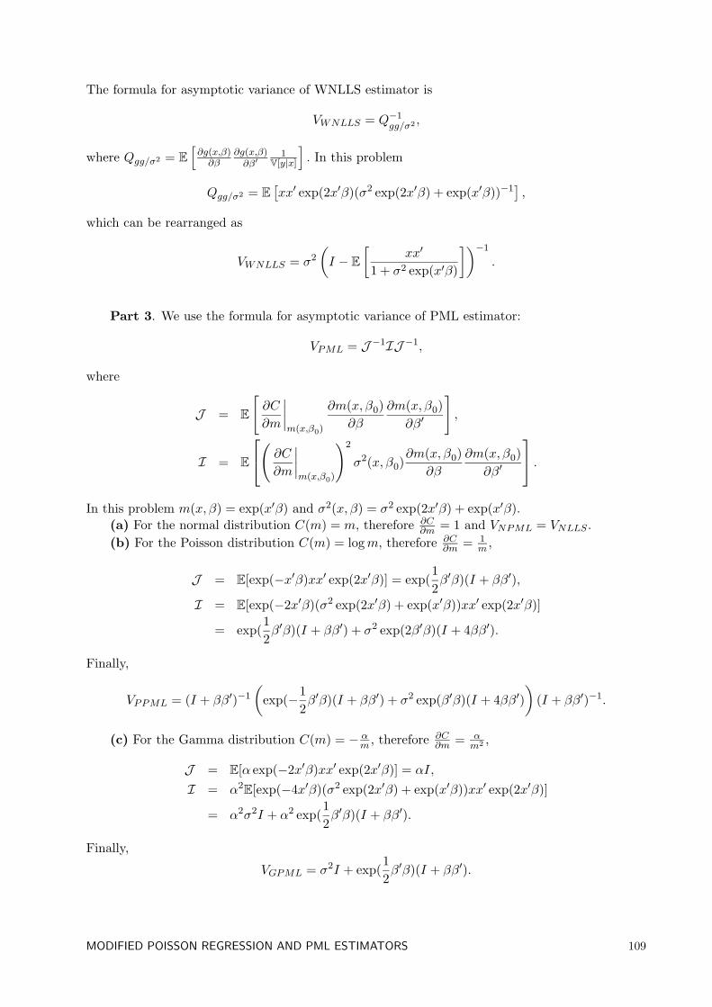
The formula for asymptotic variance of WNLLS estimator is
VWNLLS = Q−1gg/σ2 ,
where Qgg/σ2 = E
[∂g(x,β)∂β
∂g(x,β)∂β′
1V[y|x]
]. In this problem
Qgg/σ2 = E
[xx′ exp(2x′β)(σ2 exp(2x′β) + exp(x′β))−1
],
which can be rearranged as
VWNLLS = σ2
(I − E
[xx′
1 + σ2 exp(x′β)
])−1
.
Part 3. We use the formula for asymptotic variance of PML estimator:
VPML = J −1IJ −1,
where
J = E
[∂C
∂m
∣∣∣∣m(x,β0)
∂m(x, β0)∂β
∂m(x, β0)∂β′
],
I = E
( ∂C
∂m
∣∣∣∣m(x,β0)
)2
σ2(x, β0)∂m(x, β0)
∂β
∂m(x, β0)∂β′
.In this problem m(x, β) = exp(x′β) and σ2(x, β) = σ2 exp(2x′β) + exp(x′β).
(a) For the normal distribution C(m) = m, therefore ∂C∂m = 1 and VNPML = VNLLS .
(b) For the Poisson distribution C(m) = logm, therefore ∂C∂m = 1
m ,
J = E[exp(−x′β)xx′ exp(2x′β)] = exp(12β′β)(I + ββ′),
I = E[exp(−2x′β)(σ2 exp(2x′β) + exp(x′β))xx′ exp(2x′β)]
= exp(12β′β)(I + ββ′) + σ2 exp(2β′β)(I + 4ββ′).
Finally,
VPPML = (I + ββ′)−1
(exp(−1
2β′β)(I + ββ′) + σ2 exp(β′β)(I + 4ββ′)
)(I + ββ′)−1.
(c) For the Gamma distribution C(m) = − αm , therefore ∂C
∂m = αm2 ,
J = E[α exp(−2x′β)xx′ exp(2x′β)] = αI,
I = α2E[exp(−4x′β)(σ2 exp(2x′β) + exp(x′β))xx′ exp(2x′β)]
= α2σ2I + α2 exp(12β′β)(I + ββ′).
Finally,
VGPML = σ2I + exp(12β′β)(I + ββ′).
MODIFIED POISSON REGRESSION AND PML ESTIMATORS 109
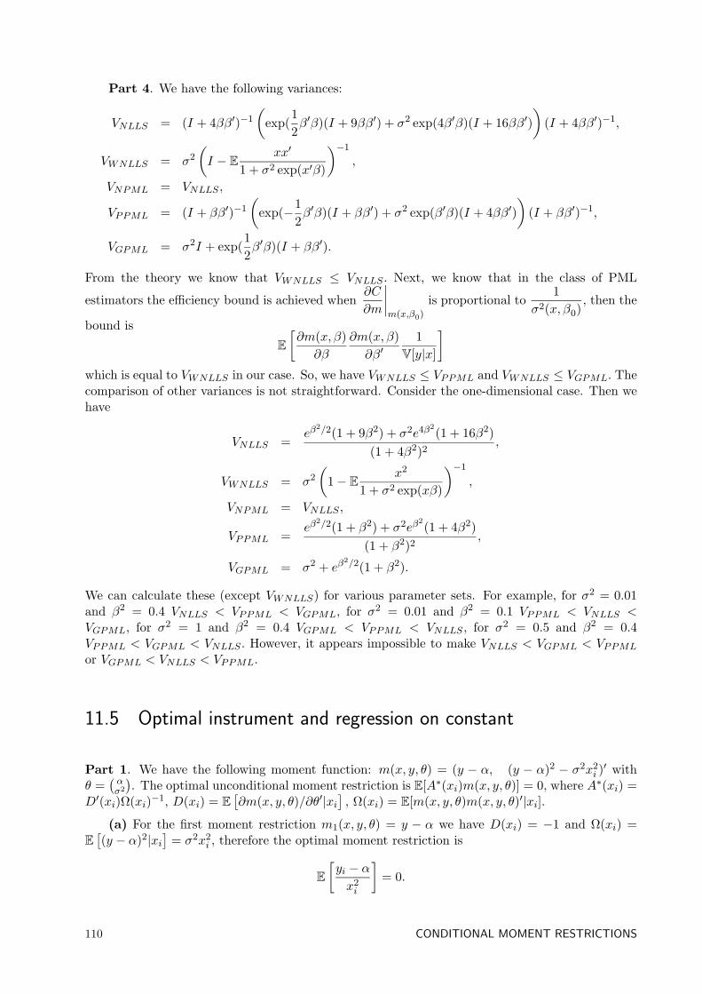
Part 4. We have the following variances:
VNLLS = (I + 4ββ′)−1
(exp(
12β′β)(I + 9ββ′) + σ2 exp(4β′β)(I + 16ββ′)
)(I + 4ββ′)−1,
VWNLLS = σ2
(I − E xx′
1 + σ2 exp(x′β)
)−1
,
VNPML = VNLLS ,
VPPML = (I + ββ′)−1
(exp(−1
2β′β)(I + ββ′) + σ2 exp(β′β)(I + 4ββ′)
)(I + ββ′)−1,
VGPML = σ2I + exp(12β′β)(I + ββ′).
From the theory we know that VWNLLS ≤ VNLLS . Next, we know that in the class of PML
estimators the efficiency bound is achieved when∂C
∂m
∣∣∣∣m(x,β0)
is proportional to1
σ2(x, β0), then the
bound is
E
[∂m(x, β)
∂β
∂m(x, β)∂β′
1V[y|x]
]which is equal to VWNLLS in our case. So, we have VWNLLS ≤ VPPML and VWNLLS ≤ VGPML. Thecomparison of other variances is not straightforward. Consider the one-dimensional case. Then wehave
VNLLS =eβ
2/2(1 + 9β2) + σ2e4β2(1 + 16β2)
(1 + 4β2)2,
VWNLLS = σ2
(1− E x2
1 + σ2 exp(xβ)
)−1
,
VNPML = VNLLS ,
VPPML =eβ
2/2(1 + β2) + σ2eβ2(1 + 4β2)
(1 + β2)2,
VGPML = σ2 + eβ2/2(1 + β2).
We can calculate these (except VWNLLS) for various parameter sets. For example, for σ2 = 0.01and β2 = 0.4 VNLLS < VPPML < VGPML, for σ2 = 0.01 and β2 = 0.1 VPPML < VNLLS <VGPML, for σ2 = 1 and β2 = 0.4 VGPML < VPPML < VNLLS , for σ2 = 0.5 and β2 = 0.4VPPML < VGPML < VNLLS . However, it appears impossible to make VNLLS < VGPML < VPPML
or VGPML < VNLLS < VPPML.
11.5 Optimal instrument and regression on constant
Part 1. We have the following moment function: m(x, y, θ) = (y − α, (y − α)2 − σ2x2i )′ with
θ =(ασ2
). The optimal unconditional moment restriction is E[A∗(xi)m(x, y, θ)] = 0, where A∗(xi) =
D′(xi)Ω(xi)−1, D(xi) = E
[∂m(x, y, θ)/∂θ′|xi
], Ω(xi) = E[m(x, y, θ)m(x, y, θ)′|xi].
(a) For the first moment restriction m1(x, y, θ) = y − α we have D(xi) = −1 and Ω(xi) =E
[(y − α)2|xi
]= σ2x2
i , therefore the optimal moment restriction is
E
[yi − αx2i
]= 0.
110 CONDITIONAL MOMENT RESTRICTIONS
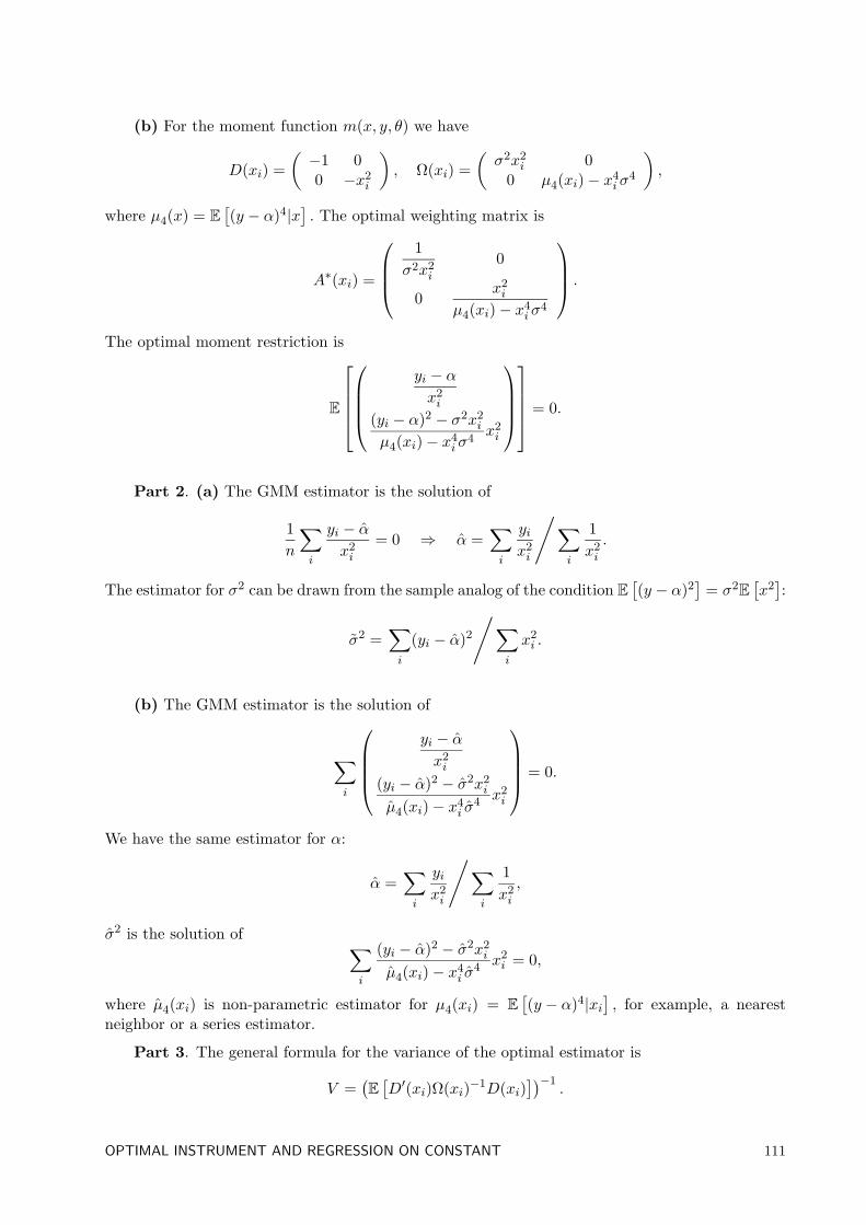
(b) For the moment function m(x, y, θ) we have
D(xi) =(−1 00 −x2
i
), Ω(xi) =
(σ2x2
i 00 µ4(xi)− x4
iσ4
),
where µ4(x) = E
[(y − α)4|x
]. The optimal weighting matrix is
A∗(xi) =
1
σ2x2i
0
0x2i
µ4(xi)− x4iσ
4
.
The optimal moment restriction is
E
yi − αx2i
(yi − α)2 − σ2x2i
µ4(xi)− x4iσ
4x2i
= 0.
Part 2. (a) The GMM estimator is the solution of
1n
∑i
yi − αx2i
= 0 ⇒ α =∑i
yix2i
/∑i
1x2i
.
The estimator for σ2 can be drawn from the sample analog of the condition E[(y − α)2
]= σ2
E
[x2]:
σ2 =∑i
(yi − α)2
/∑i
x2i .
(b) The GMM estimator is the solution of
∑i
yi − αx2i
(yi − α)2 − σ2x2i
µ4(xi)− x4i σ
4 x2i
= 0.
We have the same estimator for α:
α =∑i
yix2i
/∑i
1x2i
,
σ2 is the solution of ∑i
(yi − α)2 − σ2x2i
µ4(xi)− x4i σ
4 x2i = 0,
where µ4(xi) is non-parametric estimator for µ4(xi) = E
[(y − α)4|xi
], for example, a nearest
neighbor or a series estimator.
Part 3. The general formula for the variance of the optimal estimator is
V =(E
[D′(xi)Ω(xi)−1D(xi)
])−1.
OPTIMAL INSTRUMENT AND REGRESSION ON CONSTANT 111
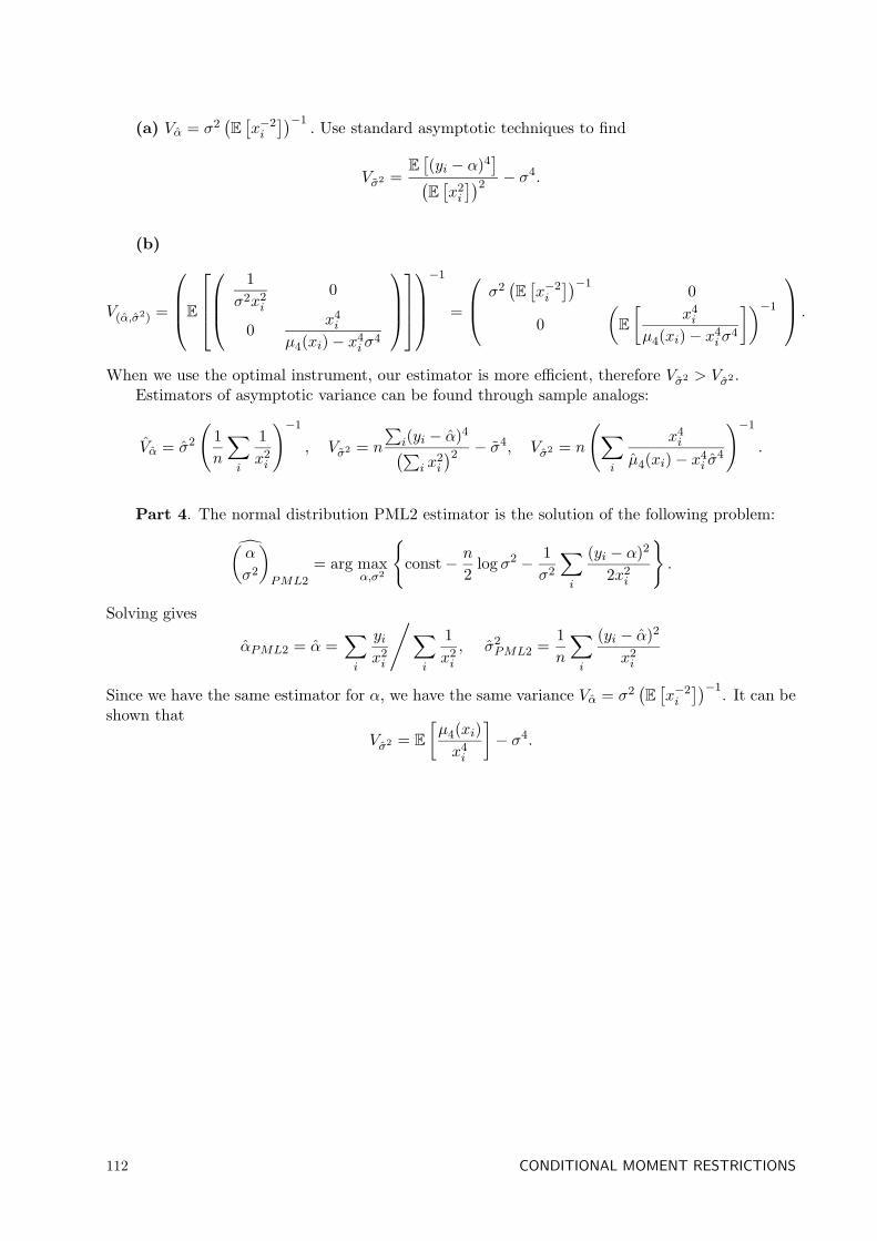
(a) Vα = σ2(E
[x−2i
])−1. Use standard asymptotic techniques to find
Vσ2 =E
[(yi − α)4
](E
[x2i
])2 − σ4.
(b)
V(α,σ2) =
E
1σ2x2
i
0
0x4i
µ4(xi)− x4iσ
4
−1
=
σ2(E
[x−2i
])−1 0
0(E
[x4i
µ4(xi)− x4iσ
4
])−1
.
When we use the optimal instrument, our estimator is more efficient, therefore Vσ2 > Vσ2 .Estimators of asymptotic variance can be found through sample analogs:
Vα = σ2
(1n
∑i
1x2i
)−1
, Vσ2 = n
∑i(yi − α)4(∑
i x2i
)2 − σ4, Vσ2 = n
(∑i
x4i
µ4(xi)− x4i σ
4
)−1
.
Part 4. The normal distribution PML2 estimator is the solution of the following problem:(α
σ2
)PML2
= arg maxα,σ2
const− n
2log σ2 − 1
σ2
∑i
(yi − α)2
2x2i
.
Solving gives
αPML2 = α =∑i
yix2i
/∑i
1x2i
, σ2PML2 =
1n
∑i
(yi − α)2
x2i
Since we have the same estimator for α, we have the same variance Vα = σ2(E
[x−2i
])−1. It can beshown that
Vσ2 = E
[µ4(xi)x4i
]− σ4.
112 CONDITIONAL MOMENT RESTRICTIONS
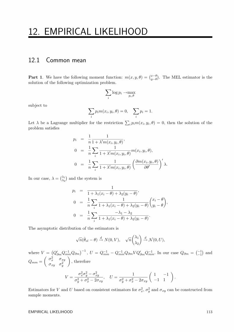
12. EMPIRICAL LIKELIHOOD
12.1 Common mean
Part 1. We have the following moment function: m(x, y, θ) =(x−θy−θ). The MEL estimator is the
solution of the following optimization problem.∑i
log pi →maxpi,θ
subject to ∑i
pim(xi, yi, θ) = 0,∑i
pi = 1.
Let λ be a Lagrange multiplier for the restriction∑
i pim(xi, yi, θ) = 0, then the solution of theproblem satisfies
pi =1n
11 + λ′m(xi, yi, θ)
,
0 =1n
∑i
11 + λ′m(xi, yi, θ)
m(xi, yi, θ),
0 =1n
∑i
11 + λ′m(xi, yi, θ)
(∂m(xi, yi, θ)
∂θ′
)′λ.
In our case, λ =(λ1
λ2
)and the system is
pi =1
1 + λ1(xi − θ) + λ2(yi − θ),
0 =1n
∑i
11 + λ1(xi − θ) + λ2(yi − θ)
(xi − θyi − θ
),
0 =1n
∑i
−λ1 − λ2
1 + λ1(xi − θ) + λ2(yi − θ).
The asymptotic distribution of the estimators is
√n(θel − θ)
d→ N(0, V ),√n
(λ1
λ2
)d→ N (0, U),
where V =(Q′∂mQ
−1mmQ∂m
)−1, U = Q−1
mm − Q−1mmQ∂mV Q
′∂mQ
−1mm. In our case Q∂m =
(−1−1
)and
Qmm =(σ2x σxyσxy σ2
y
), therefore
V =σ2xσ
2y − σ2
xy
σ2y + σ2
x − 2σxy, U =
1σ2y + σ2
x − 2σxy
(1 −1−1 1
).
Estimators for V and U based on consistent estimators for σ2x, σ2
y and σxy can be constructed fromsample moments.
EMPIRICAL LIKELIHOOD 113
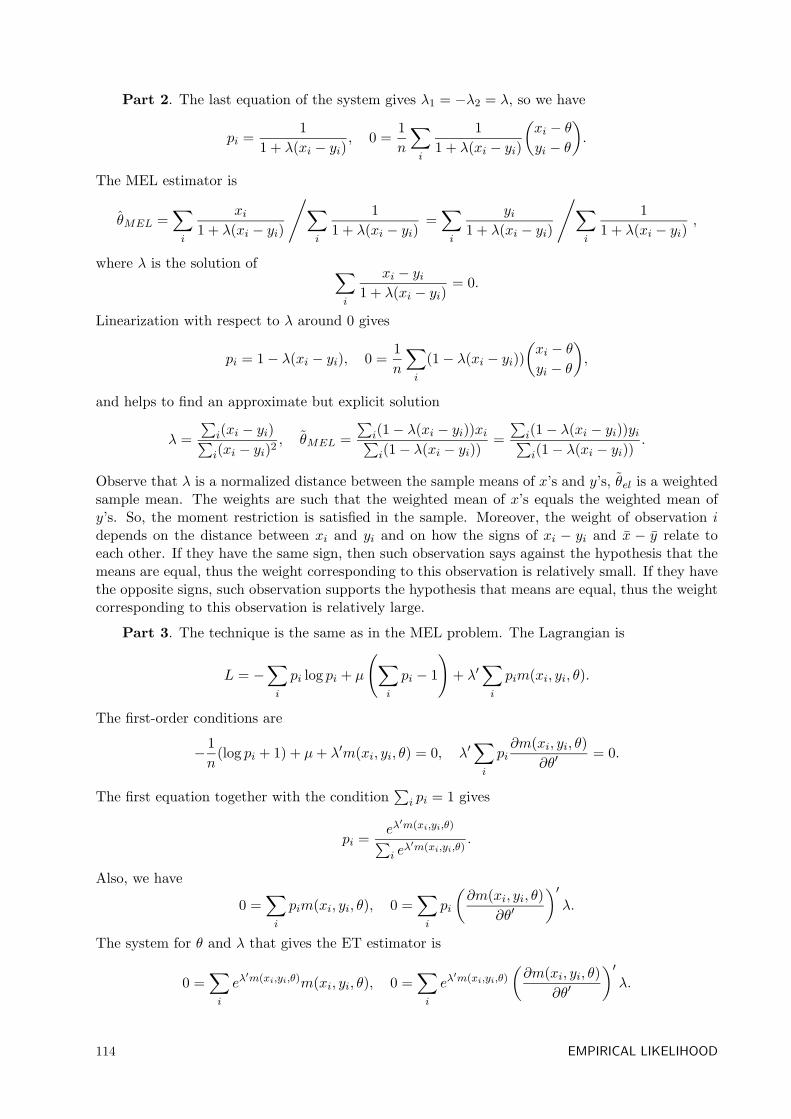
Part 2. The last equation of the system gives λ1 = −λ2 = λ, so we have
pi =1
1 + λ(xi − yi), 0 =
1n
∑i
11 + λ(xi − yi)
(xi − θyi − θ
).
The MEL estimator is
θMEL =∑i
xi1 + λ(xi − yi)
/∑i
11 + λ(xi − yi)
=∑i
yi1 + λ(xi − yi)
/∑i
11 + λ(xi − yi)
,
where λ is the solution of ∑i
xi − yi1 + λ(xi − yi)
= 0.
Linearization with respect to λ around 0 gives
pi = 1− λ(xi − yi), 0 =1n
∑i
(1− λ(xi − yi))(xi − θyi − θ
),
and helps to find an approximate but explicit solution
λ =∑
i(xi − yi)∑i(xi − yi)2
, θMEL =∑
i(1− λ(xi − yi))xi∑i(1− λ(xi − yi))
=∑
i(1− λ(xi − yi))yi∑i(1− λ(xi − yi))
.
Observe that λ is a normalized distance between the sample means of x’s and y’s, θel is a weightedsample mean. The weights are such that the weighted mean of x’s equals the weighted mean ofy’s. So, the moment restriction is satisfied in the sample. Moreover, the weight of observation idepends on the distance between xi and yi and on how the signs of xi − yi and x − y relate toeach other. If they have the same sign, then such observation says against the hypothesis that themeans are equal, thus the weight corresponding to this observation is relatively small. If they havethe opposite signs, such observation supports the hypothesis that means are equal, thus the weightcorresponding to this observation is relatively large.
Part 3. The technique is the same as in the MEL problem. The Lagrangian is
L = −∑i
pi log pi + µ
(∑i
pi − 1
)+ λ′
∑i
pim(xi, yi, θ).
The first-order conditions are
− 1n
(log pi + 1) + µ+ λ′m(xi, yi, θ) = 0, λ′∑i
pi∂m(xi, yi, θ)
∂θ′= 0.
The first equation together with the condition∑
i pi = 1 gives
pi =eλ′m(xi,yi,θ)∑
i eλ′m(xi,yi,θ)
.
Also, we have
0 =∑i
pim(xi, yi, θ), 0 =∑i
pi
(∂m(xi, yi, θ)
∂θ′
)′λ.
The system for θ and λ that gives the ET estimator is
0 =∑i
eλ′m(xi,yi,θ)m(xi, yi, θ), 0 =
∑i
eλ′m(xi,yi,θ)
(∂m(xi, yi, θ)
∂θ′
)′λ.
114 EMPIRICAL LIKELIHOOD
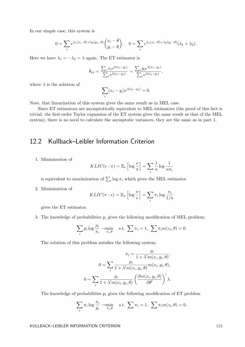
In our simple case, this system is
0 =∑i
eλ1(xi−θ)+λ2(yi−θ)(xi − θyi − θ
), 0 =
∑i
eλ1(xi−θ)+λ2(yi−θ)(λ1 + λ2).
Here we have λ1 = −λ2 = λ again. The ET estimator is
θet =∑
i xieλ(xi−yi)∑
i eλ(xi−yi)
=∑
i yieλ(xi−yi)∑
i eλ(xi−yi)
,
where λ is the solution of ∑i
(xi − yi)eλ(xi−yi) = 0.
Note, that linearization of this system gives the same result as in MEL case.Since ET estimators are asymptotically equivalent to MEL estimators (the proof of this fact is
trivial: the first-order Taylor expansion of the ET system gives the same result as that of the MELsystem), there is no need to calculate the asymptotic variances, they are the same as in part 1.
12.2 Kullback–Leibler Information Criterion
1. Minimization ofKLIC(e : π) = Ee
[log
e
π
]=∑i
1n
log1nπi
is equivalent to maximization of∑
i log πi which gives the MEL estimator.
2. Minimization ofKLIC(π : e) = Eπ
[log
π
e
]=∑i
πi logπi
1/n
gives the ET estimator.
3. The knowledge of probabilities pi gives the following modification of MEL problem:∑i
pi logpiπi→min
πi,θs.t.
∑πi = 1,
∑πim(zi, θ) = 0.
The solution of this problem satisfies the following system:
πi =pi
1 + λ′m(xi, yi, θ),
0 =∑i
pi1 + λ′m(xi, yi, θ)
m(xi, yi, θ),
0 =∑i
pi1 + λ′m(xi, yi, θ)
(∂m(xi, yi, θ)
∂θ′
)′λ.
The knowledge of probabilities pi gives the following modification of ET problem∑i
πi logπipi→min
πi,θs.t.
∑πi = 1,
∑πim(zi, θ) = 0.
KULLBACK–LEIBLER INFORMATION CRITERION 115
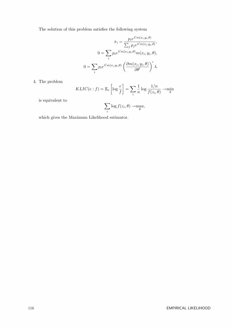
The solution of this problem satisfies the following system
πi =pie
λ′m(xi,yi,θ)∑j pje
λ′m(xj ,yj ,θ),
0 =∑i
pieλ′m(xi,yi,θ)m(xi, yi, θ),
0 =∑i
pieλ′m(xi,yi,θ)
(∂m(xi, yi, θ)
∂θ′
)′λ.
4. The problem
KLIC(e : f) = Ee
[log
e
f
]=∑i
1n
log1/n
f(zi, θ)→min
θ
is equivalent to ∑i
log f(zi, θ)→maxθ,
which gives the Maximum Likelihood estimator.
116 EMPIRICAL LIKELIHOOD