Advanced Control of Future ElectricPropulsion Systems for PassengerVehiclesMaster’s thesis in Automotive Engineering

VIGNESH ARUMUGAM SUBBIAHYASHASVI NANDIVADA

Department of Mechanics and Maritime SciencesCHALMERS UNIVERSITY OF TECHNOLOGYGoteborg, Sweden 2018

MASTER’S THESIS IN AUTOMOTIVE ENGINEERING

Advanced Control of Future Electric Propulsion Systems for PassengerVehicles

VIGNESH ARUMUGAM SUBBIAHYASHASVI NANDIVADA

Department of Mechanics and Maritime SciencesDivision of Vehicle Engineering and Autonomous Systems

CHALMERS UNIVERSITY OF TECHNOLOGY

Goteborg, Sweden 2018

Advanced Control of Future Electric Propulsion Systems for Passenger VehiclesVIGNESH ARUMUGAM SUBBIAHYASHASVI NANDIVADA

c© VIGNESH ARUMUGAM SUBBIAH, YASHASVI NANDIVADA, 2018Industrial Supervisor: Gunnar Olsson and Stefan Karlstrom, at AF Industry, TrollhattanExaminer: Mathias Lidberg, Associate Professor, Vehicle Dynamics Group, Chalmers University, Gothenburg

Master’s thesis 2018:40Department of Mechanics and Maritime SciencesDivision of Vehicle Engineering and Autonomous SystemsChalmers University of TechnologySE-412 96 GoteborgSwedenTelephone: +46 (0)31-772 1000

Cover:A BMW i3 Chassis with the high-voltage lithium-ion battery — Source Credits: BMW UK, https://discover.bmw.co.uk

Chalmers ReproserviceGoteborg, Sweden 2018

Advanced Control of Future Electric Propulsion Systems for Passenger VehiclesIndustrial Supervisor: Gunnar Olsson and Stefan Karlstrom, at AF Industry, TrollhattanMaster’s thesis in Automotive EngineeringVIGNESH ARUMUGAM SUBBIAHYASHASVI NANDIVADADepartment of Mechanics and Maritime SciencesDivision of Vehicle Engineering and Autonomous SystemsChalmers University of Technology

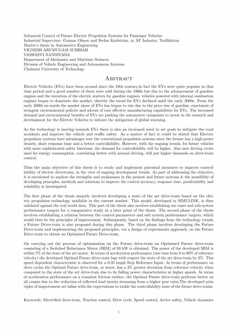
Abstract

Electric Vehicles (EVs) have been around since the 19th century,in fact the EVs were quite popular in thattime period and a good number of them were sold during the 1900s but due to the advancement of gasolineengines and the invention of the electric starters for gasoline engines, vehicles powered with internal combustionengines began to dominate the market, thereby the trend for EVs declined until the early 2000s. From theearly 2000s on-wards the market share of EVs has begun to rise due to the price rise of gasoline, enactment ofstringent environmental policies and advent of cost effective manufacturing capabilities for EVs. The increaseddemand and environmental benefits of EVs are pushing the automotive companies to invest in the research anddevelopment for the Electric Vehicles to initiate the mitigation of global warming.

As the technology is moving towards EVs there is also an increased need to set goals to mitigate the roadaccidents and improve the vehicle and traffic safety. As a matter of fact it could be stated that Electricpropulsion systems have advantages over the conventional propulsion systems since the former has a high-powerdensity, short response time and a better controllability. However, with the ongoing trends, for future vehicleswith more sophisticated safety functions, the demand for controllability will be higher. Also new driving cyclesused for energy consumption, correlating better with normal driving, will put higher demands on drive-traincontrol.

Thus the main objective of this thesis is to study and implement potential measures to improve control-lability of electric drivetrains, in the view of ongoing development trends. As part of addressing the objective,it is envisioned to analyse the strengths and weaknesses in the present and future systems & the possibility ofdeveloping principles, methods and solutions to improve the control accuracy, response time, predictability andreliability is investigated.

The first phase of the thesis majorly involved developing a state of the art drive-train based on the elec-tric propulsion technology available in the current market. This model, developed in SIMULINK, is thenvalidated against the real world data. This part of the thesis also involves establishing use cases and sub-systemperformance targets for a comparative study at a later point of the thesis. The second phase of the thesisinvolves establishing a relation between the control parameters and sub system performance targets, whichwould then be the principles of improvement. Subsequently, based on the findings from the technology trends,a Future Drive-train is also proposed during this phase. The third phase involves developing the FutureDrive-train and implementing the proposed principles, via a design of experiments approach, on the FutureDrive-train to obtain an Optimised Future Drive-train.

On carrying out the process of optimisation on the Future drive-train an Optimised Future drive-trainconsisting of a Switched Reluctance Motor (SRM) of 93 kW is obtained. The power of the developed SRM iswithin 7% of the state of the art motor. In terms of acceleration performance (rise time from 0 to 90% of referencevelocity) the developed Optimal Future drive-train lags with respect the state of the art drive-train by 2%. Thisspeed dependent characteristic is observed for a 0-35 kmph Step Reference Input. In terms of performance ondrive cycles the Optimal Future drive-train, at worst, has a 3% greater deviation from reference velocity whencompared to the state of the art drive-train due to its falling power characteristics at higher speeds. In termsof acceleration performance on a transient friction surface, the Optimal Future drive-train performs better onall counts due to the reduction of reflected load inertia stemming from a higher gear ratio.The developed prin-ciples of improvement are inline with the expectations to tackle the controllability issue of the future drive-trains.

Keywords: Electrified drive-train, Traction control, Drive cycle, Speed control, Active safety, Vehicle dynamics

i

Acknowledgements

This thesis was carried out at AF Industry and the division of Vehicle Engineering and Automotive Systemsat Chalmers University of Technology. We would like to thank our examiner Mathias Lidberg and IndustrialSupervisors Gunnar Olsson and Stefan Karlstrom for their continuous support throughout the thesis, especiallyfor their technical inputs and constructive feedback and helping us understand and implement the thesisdeliverables. We also thank Lennart Hasselqvist, the Business Unit Manager - MA Automotive R&D, JanTammpere, the Section Manager - Chassis and Vehicle Dynamics and Nicklas Karlsson, the Section Manager -Electricals for their invaluable suggestions during the Gate Presentations. Last but not least we want to thankIngrid Sjunnesson, Rudolf Brziak and Christopher Routledge from AF for their input and suggestions.

ii

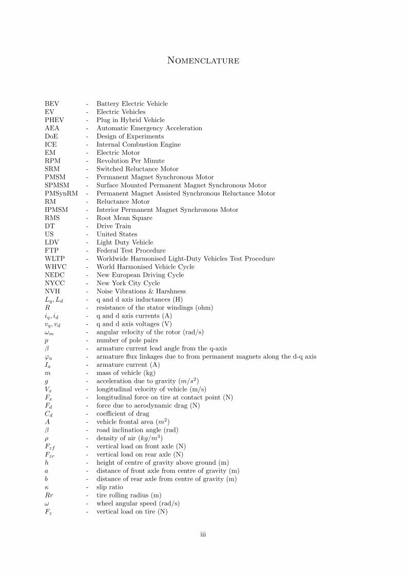
Nomenclature

BEV - Battery Electric VehicleEV - Electric VehiclesPHEV - Plug in Hybrid VehicleAEA - Automatic Emergency AccelerationDoE - Design of ExperimentsICE - Internal Combustion EngineEM - Electric MotorRPM - Revolution Per MinuteSRM - Switched Reluctance MotorPMSM - Permanent Magnet Synchronous MotorSPMSM - Surface Mounted Permanent Magnet Synchronous MotorPMSynRM - Permanent Magnet Assisted Synchronous Reluctance MotorRM - Reluctance MotorIPMSM - Interior Permanent Magnet Synchronous MotorRMS - Root Mean SquareDT - Drive TrainUS - United StatesLDV - Light Duty VehicleFTP - Federal Test ProcedureWLTP - Worldwide Harmonised Light-Duty Vehicles Test ProcedureWHVC - World Harmonised Vehicle CycleNEDC - New European Driving CycleNYCC - New York City CycleNVH - Noise Vibrations & HarshnessLq, Ld - q and d axis inductances (H)R - resistance of the stator windings (ohm)iq, id - q and d axis currents (A)vq, vd - q and d axis voltages (V)ωm - angular velocity of the rotor (rad/s)p - number of pole pairsβ - armature current lead angle from the q-axisϕa - armature flux linkages due to from permanent magnets along the d-q axisIa - armature current (A)m - mass of vehicle (kg)g - acceleration due to gravity (m/s2)Vx - longitudinal velocity of vehicle (m/s)Fx - longitudinal force on tire at contact point (N)Fd - force due to aerodynamic drag (N)Cd - coefficient of dragA - vehicle frontal area (m2)β - road inclination angle (rad)ρ - density of air (kg/m3)Fzf - vertical load on front axle (N)Fzr - vertical load on rear axle (N)h - height of centre of gravity above ground (m)a - distance of front axle from centre of gravity (m)b - distance of rear axle from centre of gravity (m)κ - slip ratioRr - tire rolling radius (m)ω - wheel angular speed (rad/s)Fz - vertical load on tire (N)

iii

B,C,D,E - magic tire formula coefficientsN - gear ratiorf - radius of follower gear (m)rb - radius of base gear (m)τb - torque acting on base gear (Nm)τf - torque acting on follower gear (Nm)τloss - losses in torque transfer calculated based on the efficiency parameter (Nm)ωf - follower gear angular velocity (rad/s)ωb - base gear angular velocity (rad/s)Jf - follower gear inertia (kgm2)Jb - base gear inertia (kgm2)error - velocity error (input to the controller)Vreference - reference/target velocity for the vehicle (m/s)P - proportional gainD - differential gainλ - amplitude of the flux induced by the permanent magnets of the rotor in the stator phases (Vs)Te - electromagnetic torque (Nm)θe - rotor angle (rad)Tph - torque generated by one phase (Nm)Ψph - magnetic flux linkage (Vs)θph - rotor angle (degree)iph - phase current (A)Vph - phase voltage (V)Rph - phase resistance (ohm)Tf - shaft static friction torque (Nm)Tm - shaft mechanical torque (Nm)F - combined viscous friction of rotor and loadJ - combined rotor and load inertia (kgm2)TM - motor torque (Nm)JM - motor inertia (kgm2)JL - load inertia (kgm2)J∗L - load inertia including gear-box inertia (kgm2)JGB - gear box inertia (kgm2)Jt - total reflected inertia (kgm2)NM - number of teeth on base gear wheelNL - number of teeth on follower gear wheel

iv

Contents

Abstract i

Acknowledgements ii

Nomenclature iii

Contents v

1 Introduction 11.1 Background . . . . . . . . . . . . . . . . . . . . . . . . . . . . . . . . . . . . . . . . . . . . . . . . . 11.2 Motivation for the Project . . . . . . . . . . . . . . . . . . . . . . . . . . . . . . . . . . . . . . . . . 31.3 Objective and Envisioned Solution . . . . . . . . . . . . . . . . . . . . . . . . . . . . . . . . . . . . 31.4 Deliverables . . . . . . . . . . . . . . . . . . . . . . . . . . . . . . . . . . . . . . . . . . . . . . . . . 31.5 Delimitations . . . . . . . . . . . . . . . . . . . . . . . . . . . . . . . . . . . . . . . . . . . . . . . . 41.6 Work Procedure and Methodology . . . . . . . . . . . . . . . . . . . . . . . . . . . . . . . . . . . . 4

2 Technology Review 72.1 Literature Review . . . . . . . . . . . . . . . . . . . . . . . . . . . . . . . . . . . . . . . . . . . . . 72.1.1 Electric Vehicle Database . . . . . . . . . . . . . . . . . . . . . . . . . . . . . . . . . . . . . . . . 72.1.2 Drive Cycles & Manoeuvres . . . . . . . . . . . . . . . . . . . . . . . . . . . . . . . . . . . . . . . 72.1.3 Market Trends . . . . . . . . . . . . . . . . . . . . . . . . . . . . . . . . . . . . . . . . . . . . . . 82.1.4 Powertrain Technology . . . . . . . . . . . . . . . . . . . . . . . . . . . . . . . . . . . . . . . . . . 102.1.5 Control and Power Electronics . . . . . . . . . . . . . . . . . . . . . . . . . . . . . . . . . . . . . 152.2 Technology Analysis . . . . . . . . . . . . . . . . . . . . . . . . . . . . . . . . . . . . . . . . . . . . 162.2.1 E-Motor Technology . . . . . . . . . . . . . . . . . . . . . . . . . . . . . . . . . . . . . . . . . . . 162.2.2 Transmission Technology . . . . . . . . . . . . . . . . . . . . . . . . . . . . . . . . . . . . . . . . 172.3 Priori for DoE . . . . . . . . . . . . . . . . . . . . . . . . . . . . . . . . . . . . . . . . . . . . . . . 182.3.1 Intro to DoE . . . . . . . . . . . . . . . . . . . . . . . . . . . . . . . . . . . . . . . . . . . . . . . 182.3.2 Adopted Experimental Design Setup . . . . . . . . . . . . . . . . . . . . . . . . . . . . . . . . . . 192.3.3 Model Fitting & Optimisation . . . . . . . . . . . . . . . . . . . . . . . . . . . . . . . . . . . . . 19

3 Selection of Use Cases 213.1 Cruise Control . . . . . . . . . . . . . . . . . . . . . . . . . . . . . . . . . . . . . . . . . . . . . . . 213.2 Drive Cycles . . . . . . . . . . . . . . . . . . . . . . . . . . . . . . . . . . . . . . . . . . . . . . . . 213.2.1 NEDC . . . . . . . . . . . . . . . . . . . . . . . . . . . . . . . . . . . . . . . . . . . . . . . . . . . 223.2.2 US06 . . . . . . . . . . . . . . . . . . . . . . . . . . . . . . . . . . . . . . . . . . . . . . . . . . . 233.2.3 WLTP Class 3 . . . . . . . . . . . . . . . . . . . . . . . . . . . . . . . . . . . . . . . . . . . . . . 233.3 Traction Control Use Case . . . . . . . . . . . . . . . . . . . . . . . . . . . . . . . . . . . . . . . . . 23

4 Vehicle and Drive-train Parameterisation 254.1 Vehicle Model . . . . . . . . . . . . . . . . . . . . . . . . . . . . . . . . . . . . . . . . . . . . . . . . 254.1.1 Vehicle Body . . . . . . . . . . . . . . . . . . . . . . . . . . . . . . . . . . . . . . . . . . . . . . . 254.1.2 Wheels & Tires . . . . . . . . . . . . . . . . . . . . . . . . . . . . . . . . . . . . . . . . . . . . . . 254.1.3 Transmission . . . . . . . . . . . . . . . . . . . . . . . . . . . . . . . . . . . . . . . . . . . . . . . 264.1.4 Open Differential . . . . . . . . . . . . . . . . . . . . . . . . . . . . . . . . . . . . . . . . . . . . . 264.1.5 Battery . . . . . . . . . . . . . . . . . . . . . . . . . . . . . . . . . . . . . . . . . . . . . . . . . . 264.1.6 Vehicle Controllers . . . . . . . . . . . . . . . . . . . . . . . . . . . . . . . . . . . . . . . . . . . . 264.1.7 Power Electronics . . . . . . . . . . . . . . . . . . . . . . . . . . . . . . . . . . . . . . . . . . . . 274.2 State of the Art Drive-train . . . . . . . . . . . . . . . . . . . . . . . . . . . . . . . . . . . . . . . . 294.2.1 Motor . . . . . . . . . . . . . . . . . . . . . . . . . . . . . . . . . . . . . . . . . . . . . . . . . . . 304.2.2 Motor Controller . . . . . . . . . . . . . . . . . . . . . . . . . . . . . . . . . . . . . . . . . . . . . 314.3 Proposed Future Drive-train . . . . . . . . . . . . . . . . . . . . . . . . . . . . . . . . . . . . . . . . 314.3.1 Motor . . . . . . . . . . . . . . . . . . . . . . . . . . . . . . . . . . . . . . . . . . . . . . . . . . . 324.3.2 Motor Controller . . . . . . . . . . . . . . . . . . . . . . . . . . . . . . . . . . . . . . . . . . . . . 33

v

4.4 Simulation Challenges & Solutions . . . . . . . . . . . . . . . . . . . . . . . . . . . . . . . . . . . . 334.5 Design of Experiments and Parameterisation . . . . . . . . . . . . . . . . . . . . . . . . . . . . . . 34

5 Results 375.1 DoE and Optimisation of Future Drive-train . . . . . . . . . . . . . . . . . . . . . . . . . . . . . . 375.2 Comparison of Motors . . . . . . . . . . . . . . . . . . . . . . . . . . . . . . . . . . . . . . . . . . . 395.3 Use Case-Cruise Control . . . . . . . . . . . . . . . . . . . . . . . . . . . . . . . . . . . . . . . . . . 415.3.1 Performance of State of the Art Drive-train . . . . . . . . . . . . . . . . . . . . . . . . . . . . . . 415.3.2 Performance of Optimised Future Drive-train . . . . . . . . . . . . . . . . . . . . . . . . . . . . . 415.3.3 Comparison and Validation . . . . . . . . . . . . . . . . . . . . . . . . . . . . . . . . . . . . . . . 425.4 Use Case-Drive Cycle . . . . . . . . . . . . . . . . . . . . . . . . . . . . . . . . . . . . . . . . . . . 445.4.1 NEDC . . . . . . . . . . . . . . . . . . . . . . . . . . . . . . . . . . . . . . . . . . . . . . . . . . . 445.4.2 US06 . . . . . . . . . . . . . . . . . . . . . . . . . . . . . . . . . . . . . . . . . . . . . . . . . . . 465.4.3 WLTP Class 3 . . . . . . . . . . . . . . . . . . . . . . . . . . . . . . . . . . . . . . . . . . . . . . 485.5 Use Case-Traction Control . . . . . . . . . . . . . . . . . . . . . . . . . . . . . . . . . . . . . . . . . 515.5.1 Performance of State of the Art Drive-train . . . . . . . . . . . . . . . . . . . . . . . . . . . . . . 515.5.2 Performance of Optimised Future Drive-train . . . . . . . . . . . . . . . . . . . . . . . . . . . . . 525.5.3 Comparison and Validation . . . . . . . . . . . . . . . . . . . . . . . . . . . . . . . . . . . . . . . 53

6 Conclusion 56

7 Future Work 57

References 58

A EV Database I

B Technology Analysis IIB.1 E - Motor . . . . . . . . . . . . . . . . . . . . . . . . . . . . . . . . . . . . . . . . . . . . . . . . . . IIB.2 Transmission . . . . . . . . . . . . . . . . . . . . . . . . . . . . . . . . . . . . . . . . . . . . . . . . IV

C Vehicle & Motor Specifications VIC.1 Vehicle Specifications . . . . . . . . . . . . . . . . . . . . . . . . . . . . . . . . . . . . . . . . . . . VIC.1.1 Vehicle Body . . . . . . . . . . . . . . . . . . . . . . . . . . . . . . . . . . . . . . . . . . . . . . . VIC.1.2 Wheels and Tires . . . . . . . . . . . . . . . . . . . . . . . . . . . . . . . . . . . . . . . . . . . . . VIC.1.3 Transmission . . . . . . . . . . . . . . . . . . . . . . . . . . . . . . . . . . . . . . . . . . . . . . . VIIIC.1.4 Open Differential . . . . . . . . . . . . . . . . . . . . . . . . . . . . . . . . . . . . . . . . . . . . . VIIIC.1.5 Cruise Controller . . . . . . . . . . . . . . . . . . . . . . . . . . . . . . . . . . . . . . . . . . . . . IXC.2 State of the Art Motor . . . . . . . . . . . . . . . . . . . . . . . . . . . . . . . . . . . . . . . . . . . IXC.3 Optimal Future Motor . . . . . . . . . . . . . . . . . . . . . . . . . . . . . . . . . . . . . . . . . . . X

D Design of Experiments XID.1 List of Experiments . . . . . . . . . . . . . . . . . . . . . . . . . . . . . . . . . . . . . . . . . . . . XI

E Motivations for Results XIIIE.1 Cruise Control Motivations . . . . . . . . . . . . . . . . . . . . . . . . . . . . . . . . . . . . . . . . XIIIE.2 Traction Control Motivations . . . . . . . . . . . . . . . . . . . . . . . . . . . . . . . . . . . . . . . XIV

vi

1 Introduction

1.1 Background

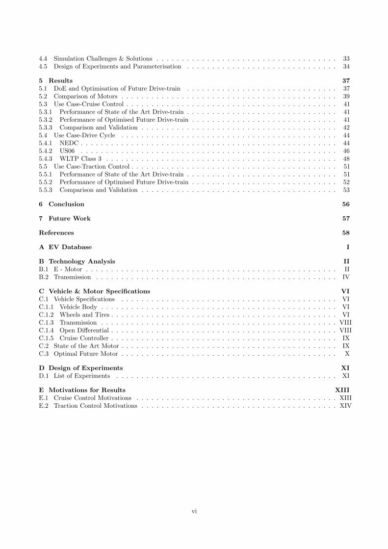
Electric vehicles (EVs) have been around since the late 1800s and their popularity has been steadily increasingever since as seen in Figure 1.1 [IE17], which depicts the growth of EVs between 2011 and 2025.This trend isexpected to hold if not increase and BEVs (Battery Electric Vehicles) are forecast to hold 60% of the totalelectric vehicle (including PHEV & HEV) sales by the year 2025, when the EV stock pile is expected to cross 7million with annual sales of over 1 million vehicles [CS17]. The increased market share and wider acceptance of

Figure 1.1: Evolution of the Global Electric Car Stock(2011-2025) [IE17]

EVs can be attributed to the factors below:

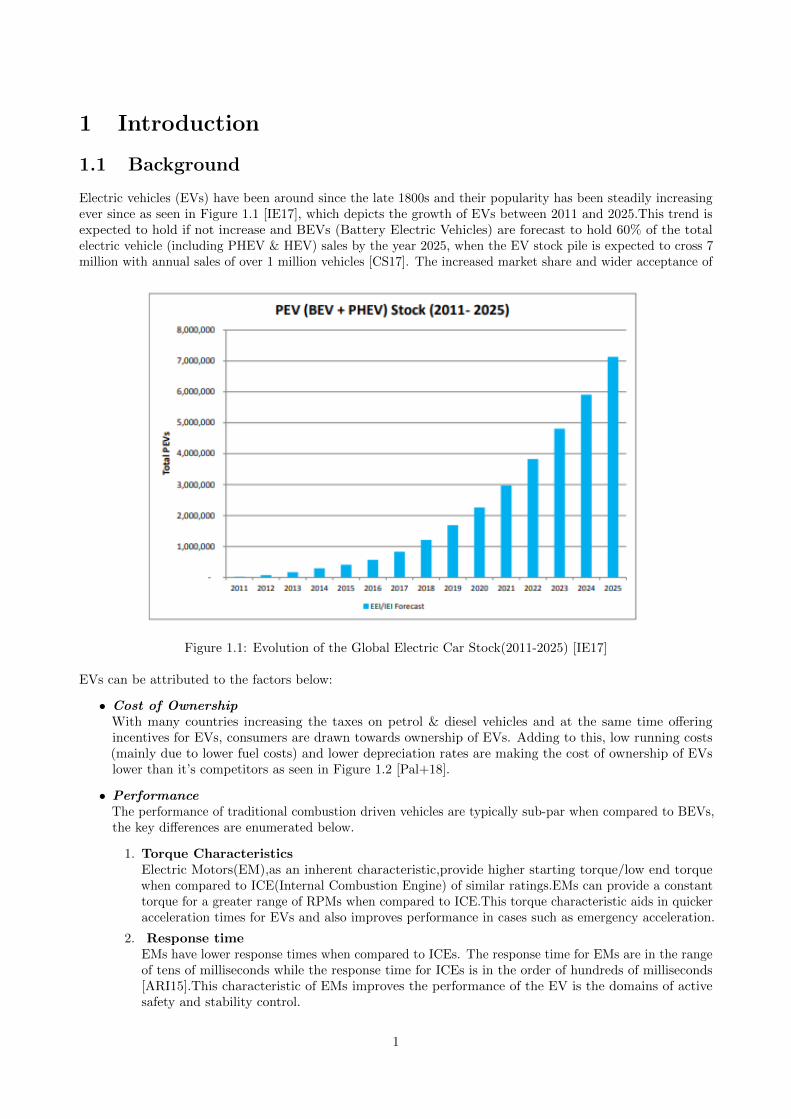
• Cost of OwnershipWith many countries increasing the taxes on petrol & diesel vehicles and at the same time offeringincentives for EVs, consumers are drawn towards ownership of EVs. Adding to this, low running costs(mainly due to lower fuel costs) and lower depreciation rates are making the cost of ownership of EVslower than it’s competitors as seen in Figure 1.2 [Pal+18].

• PerformanceThe performance of traditional combustion driven vehicles are typically sub-par when compared to BEVs,the key differences are enumerated below.

1. Torque CharacteristicsElectric Motors(EM),as an inherent characteristic,provide higher starting torque/low end torquewhen compared to ICE(Internal Combustion Engine) of similar ratings.EMs can provide a constanttorque for a greater range of RPMs when compared to ICE.This torque characteristic aids in quickeracceleration times for EVs and also improves performance in cases such as emergency acceleration.

2. Response timeEMs have lower response times when compared to ICEs. The response time for EMs are in the rangeof tens of milliseconds while the response time for ICEs is in the order of hundreds of milliseconds[ARI15].This characteristic of EMs improves the performance of the EV is the domains of activesafety and stability control.

1

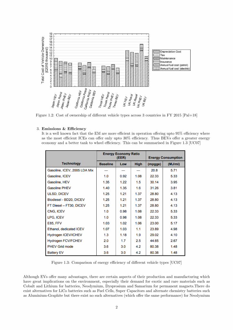
Figure 1.2: Cost of ownership of different vehicle types across 3 countries in FY 2015 [Pal+18]

3. Emissions & EfficiencyIt is a well known fact that the EM are more efficient in operation offering upto 95% efficiency whereas the most efficient ICEs can offer only upto 30% efficiency. Thus BEVs offer a greater energyeconomy and a better tank to wheel efficiency. This can be summarised in Figure 1.3 [UC07]

Figure 1.3: Comparison of energy efficiency of different vehicle types [UC07]

Although EVs offer many advantages, there are certain aspects of their production and manufacturing whichhave great implications on the environment, especially their demand for exotic and rare materials such asCobalt and Lithium for batteries, Neodymium, Dysprosium and Samarium for permanent magnets.There doexist alternatives for LiCo batteries such as Fuel Cells, Super Capacitors and alternate chemistry batteries suchas Aluminium-Graphite but there exist no such alternatives (which offer the same performance) for Neodymium

2

based permanent magnets.This is a cause for concern as:

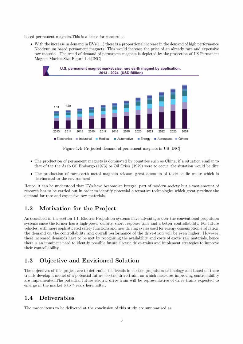
• With the increase in demand in EVs(1.1) there is a proportional increase in the demand of high performanceNeodymium based permanent magnets. This would increase the price of an already rare and expensiveraw material. The trend of demand of permanent magnets is depicted by the projection of US PermanentMagnet Market Size Figure 1.4 [INC]

Figure 1.4: Projected demand of permanent magnets in US [INC]

• The production of permanent magnets is dominated by countries such as China, if a situation similar tothat of the the Arab Oil Embargo (1973) or Oil Crisis (1979) were to occur, the situation would be dire.

• The production of rare earth metal magnets releases great amounts of toxic acidic waste which isdetrimental to the environment

Hence, it can be understood that EVs have become an integral part of modern society but a vast amount ofresearch has to be carried out in order to identify potential alternative technologies which greatly reduce thedemand for rare and expensive raw materials.

1.2 Motivation for the Project

As described in the section 1.1, Electric Propulsion systems have advantages over the conventional propulsionsystems since the former has a high-power density, short response time and a better controllability. For futurevehicles, with more sophisticated safety functions and new driving cycles used for energy consumption evaluation,the demand on the controllability and overall performance of the drive-train will be even higher. However,these increased demands have to be met by recognising the availability and costs of exotic raw materials, hencethere is an imminent need to identify possible future electric drive-trains and implement strategies to improvetheir controllability.

1.3 Objective and Envisioned Solution

The objectives of this project are to determine the trends in electric propulsion technology and based on thesetrends develop a model of a potential future electric drive-train, on which measures improving controllabilityare implemented.The potential future electric drive-train will be representative of drive-trains expected toemerge in the market 6 to 7 years hereinafter.

1.4 Deliverables

The major items to be delivered at the conclusion of this study are summarised as:

3

• A study of the technical, market and social trends in electric propulsion technology

• Define use cases e.g. real-life driving cycles (mainly US, China & Europe), and Automatic EmergencyAcceleration (AEA)

• Identify subsystem performance targets

• Develop principles for improving controllability based on identified use cases

• Demonstration of drive-trains with and without the proposed improvements on the identified use cases

1.5 Delimitations

To limit the scope of this study, certain boundaries on the field of study have been imposed:

• No vehicle configurations apart from passenger vehicles are considered

• Vehicle configurations with two driven wheels and no more than four wheels are considered

• Configurations involving hub motors are excluded

• Minimum of one and maximum of two motors are considered to propel the vehicle

• Longitudinal and straight line vehicle manoeuvres are considered

1.6 Work Procedure and Methodology

The work flow adopted can be described using the logical steps taken through the project as:

• Step 1: Literature Review, Technology Analysis and Prediction of Future Drive-trainThrough literature studies and interviews with subject matter experts, status and trends in E-motortechnology, transmissions and power electronics were determined.Further,the strengths and weaknessesof the State of the Art and future systems were identified and analysed. The conclusion of this stageincluded the realisation of:

1. Current EV technology and establishment of the State of the Art Drive-train

2. Possible development opportunities for Future Drive-train

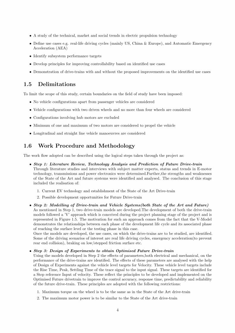
• Step 2: Modelling of Drive-train and Vehicle Systems(both State of the Art and Future)As mentioned in Step 1, two drive-train models are developed.The development of both the drive-trainmodels followed a ’V’ approach which is conceived during the project planning stage of the project and isrepresented in Figure 1.5. The motivation for such an approach comes from the fact that the V-Modeldemonstrates the relationships between each phase of the development life cycle and its associated phaseof reaching the surface level or the testing phase in this case.Once the models are developed, the use cases, on which the drive-trains are to be studied, are identified.Some of the driving scenarios of interest are real life driving cycles, emergency acceleration(to preventrear end collision), braking on low/stepped friction surface etc.

• Step 3: Design of Experiments to obtain Optimised Future Drive-trainUsing the models developed in Step 2 the effects of parameters,both electrical and mechanical, on theperformance of the drive-trains are identified. The effects of these parameters are analysed with the helpof Design of Experiments against the vehicle level targets for Velocity. These vehicle level targets includethe Rise Time, Peak, Settling Time of the trace signal to the input signal. These targets are identified fora Step reference Input of velocity. These reflect the principles to be developed and implemented on theOptimised Future drivetrain to improve the control accuracy, response time, predictability and reliabilityof the future drive-train. These principles are adopted with the following restrictions:

1. Maximum torque on the wheel is to be the same as in the State of the Art drive-train

2. The maximum motor power is to be similar to the State of the Art drive-train

4

Exploration of

Concepts and

Technology

Design of Vehicle

Level Systems

Complete Model

Implementation

Validation and

Testing of Models

Observed Response

Of Vehicle Model

Design of Subsystems

Figure 1.5: Adopted ’V’ approach for Model Development

3. The same vehicle level controllers is to be used for both drive-trains

4. The same drive-train layout is to be considered for both drive-trains

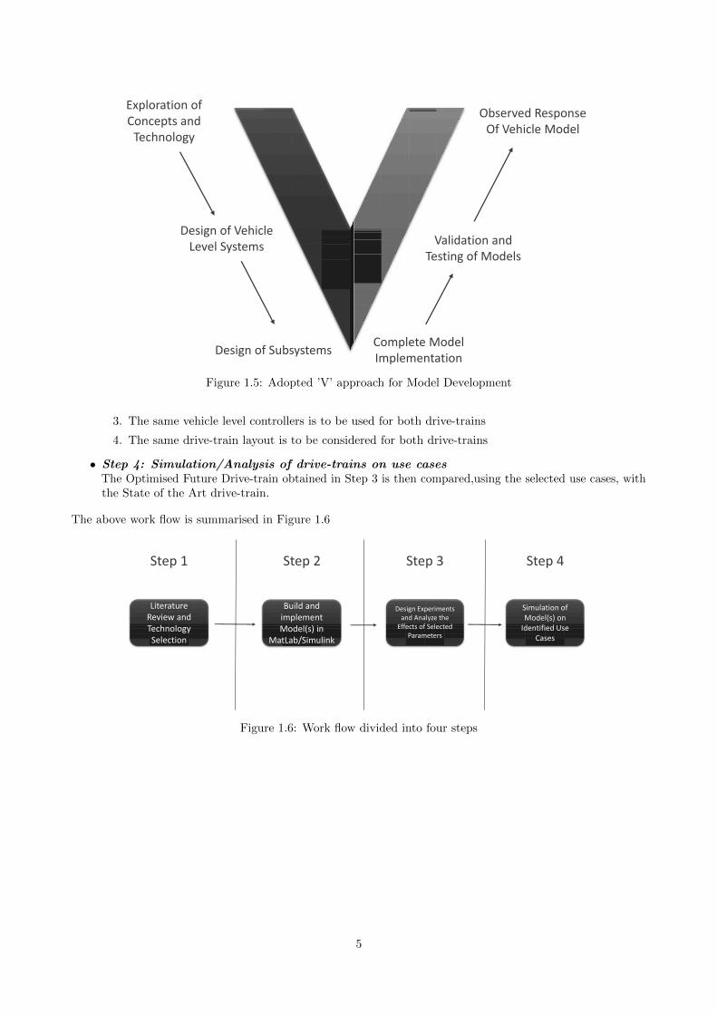
• Step 4: Simulation/Analysis of drive-trains on use casesThe Optimised Future Drive-train obtained in Step 3 is then compared,using the selected use cases, withthe State of the Art drive-train.

The above work flow is summarised in Figure 1.6

Build and

implement

Model(s) in

MatLab/Simulink

Design Experiments

and Analyze the

Effects of Selected

Parameters

Simulation of

Model(s) on

Identified Use

Cases

Literature

Review and

Technology

Selection

Step 1 Step 2 Step 3 Step 4

Figure 1.6: Work flow divided into four steps

5

6

2 Technology Review

This section briefly discusses the Literature review undertaken during the course of the thesis and the technologyanalysis pursued in order to establish a connection between the State of the Art and Future Systems. Theterms State of the Art corresponds to the Current Day Scenario in Technology.The priori for Design of Experiments is also discussed in this section, which helps understand the Analysis inthe later sections.

2.1 Literature Review

On a surface level, to understand the scope of the thesis better, the major areas of concentration are classifiedto be studied during the literature review phase. As part of this the areas of major focus are divided as below.

• Electric Vehicle Database - This section intends to identify the current State of the Art electric vehicletechnology which enables narrowing down the State of the Art Drive-train.

• Drive Cycles - This section intends to select the Drive Cycles that would put highest demand on thepowertrain, thus contributing for a better comparison. This section also establishes the base for Section 3

• Market Trends - This section intends to dwell the the factors driving the EV trend and establish theemerging and future trends.

• Powertrain Technology - This section intends to compare the existing Powertrain Technologies and discussin brief the reasons for their preference.

• Control & Power Electronics - This section briefly discusses the Power Electronics available and theirimportance in tackling the scope of this thesis.

2.1.1 Electric Vehicle Database

To understand the State of the Art scenario of Electric vehicles, it is very important to list down the specifi-cations of the vehicles available today. To simplify the search region, as established in the delimitations it isdecided to list down the Passenger Electric Vehicles. The parameters of technical importance are identified foreach vehicle and their respective values are captured.

The vehicle list here is the list of Highway Capable Passenger electric vehicles available in the market.Thevehicle database is as shown in table A.

2.1.2 Drive Cycles & Manoeuvres

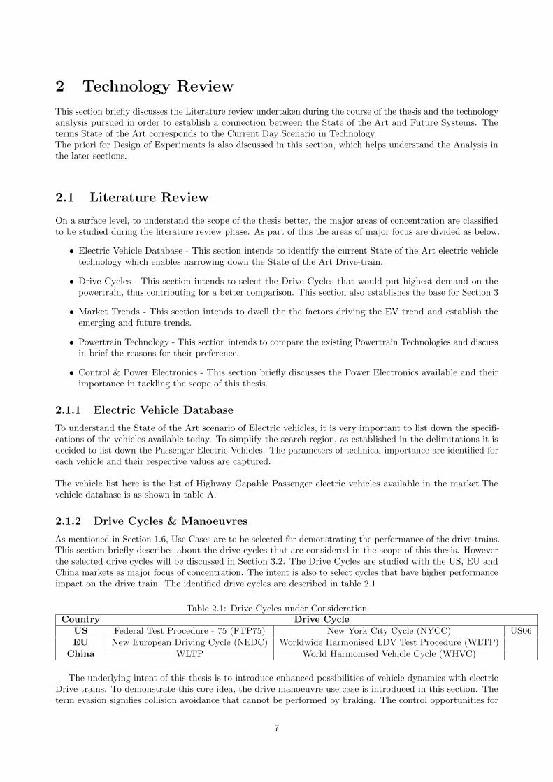
As mentioned in Section 1.6, Use Cases are to be selected for demonstrating the performance of the drive-trains.This section briefly describes about the drive cycles that are considered in the scope of this thesis. Howeverthe selected drive cycles will be discussed in Section 3.2. The Drive Cycles are studied with the US, EU andChina markets as major focus of concentration. The intent is also to select cycles that have higher performanceimpact on the drive train. The identified drive cycles are described in table 2.1

Table 2.1: Drive Cycles under ConsiderationCountry Drive Cycle

US Federal Test Procedure - 75 (FTP75) New York City Cycle (NYCC) US06EU New European Driving Cycle (NEDC) Worldwide Harmonised LDV Test Procedure (WLTP)

China WLTP World Harmonised Vehicle Cycle (WHVC)

The underlying intent of this thesis is to introduce enhanced possibilities of vehicle dynamics with electricDrive-trains. To demonstrate this core idea, the drive manoeuvre use case is introduced in this section. Theterm evasion signifies collision avoidance that cannot be performed by braking. The control opportunities for

7

0 500 1000 1500 2000 2500

Time [s]

0

5

10

15

20

25

30

Vel

ocity

[m/s

]

FTP75 Drive Cycle

Figure 2.1: FTP75 Drive Cycle

0 100 200 300 400 500 600

Time [s]

0

2

4

6

8

10

12

14

Vel

ocity

[m/s

]

NYCC Drive Cycle

Figure 2.2: NYCC Drive Cycle

0 100 200 300 400 500 600 700 800 900

Time [s]

0

2

4

6

8

10

12

14

16

18

20

Vel

ocity

[m/s

]

World Harmonized Vehicle Test Cycle

Figure 2.3: WHVC Drive Cycle

each of the manoeuvres are shown in their respective figures.The possibility of electric Drive-train intervention is briefly discussed in the Appendix.

2.1.3 Market Trends

As for the study of technology trends in the industry, McKinsey as a team with A2Mac1 [Err+17], a supplierof car benchmarking services, led an extensive scale benchmarking of first-and second-generation EV models,which included physically dismantling ten EV models: the 2011 Nissan LEAF, the 2013 Volkswagen e-up!, the2013 Tesla Model S, the 2014 Chevrolet Spark, the 2014 BMW i3, the 2015 Volkswagen e-Golf, the 2015 BYDe6, the 2017 Nissan LEAF, the 2017 Chevrolet Bolt, and the 2017 Opel Ampera-e. Together these modelsaccount for about 40 percent in the market share of Battery Electric Vehicles. This tear down analysis alongwith publicly available information and subject matter experts revealed key insights into the trend.The key insights include,

• Platform Architecture vs RangeThe benchmarking demonstrates a gap in bridging driving range and interior space between models withnative EV platform architectures and those based out of ICE platforms. OEM’s native architectureplatforms have better battery packaging where as the non-native platforms have forcefully fit batterypackaging which in turn limits the realisable energy capacity. The native EV battery pack, by far, cantake a basic, rectangular shape, making native EVs to double the range by more than 300 kilometers percharge and to roughly 400 kilometers for the best performing architectures, as per the EnvironmentalProtection Agency—without constraining up the price (2.4).Also, Native EVs accomplish a larger interiorspace (up to 10 percent by regression line) for a similar wheelbase compared to the ICE vehicles.

• Design to Cost RatioAs similar to the trends in the initial days of ICE development, OEMs are following a similar way oftackling problem for the EVs as well. Once the battle for establishing the leadership for performance andrange, OEMs are targeting the design to cost build-up in the second generation EVs being developed.This trend could be mostly noted in component integration and smarter usage of light weight materialsand avoiding over design. OEMs are trying to cut down the weight of the vehicle by leaps and bounds toachieve a better range (2.5). However there is always a limit beyond which the OEMs are not willing tocut down the weight to ensure a safe structure. This then brings us to the discussion of cutting down theweight of the powertrain. Generational leaps in powertrain technology are expected to yield significantweight reductions. This would not only reduce the weight but also the Powertrain Manufacturing costs.Although there aren’t any external incentives available today for cutting down weight in EVs, it could bea possibility in the near future thus enhancing the market.

• Competence and ComponentsThe combinations of engine transmission types are very minimal by the current EV industry, as the[Err+17] rightly says there is hardly any differentiation in performance in current EVs compared totheir ICE counterparts in the same segment. Base EV’s configurations contain many options alreadyunlike the ICEs which evolved over time. This will also imply that the small window for component level

8

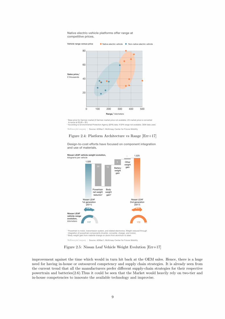
Figure 2.4: Platform Architecture vs Range [Err+17]

Figure 2.5: Nissan Leaf Vehicle Weight Evolution [Err+17]

improvement against the time which would in turn hit back at the OEM sales. Hence, there is a hugeneed for having in-house or outsourced competency and supply chain strategies. It is already seen fromthe current trend that all the manufacturers prefer different supply-chain strategies for their respectivepowertrain and batteries(2.6).Thus it could be seen that the Market would heavily rely on two-tier andin-house competencies to innovate the available technology and improvise.

9

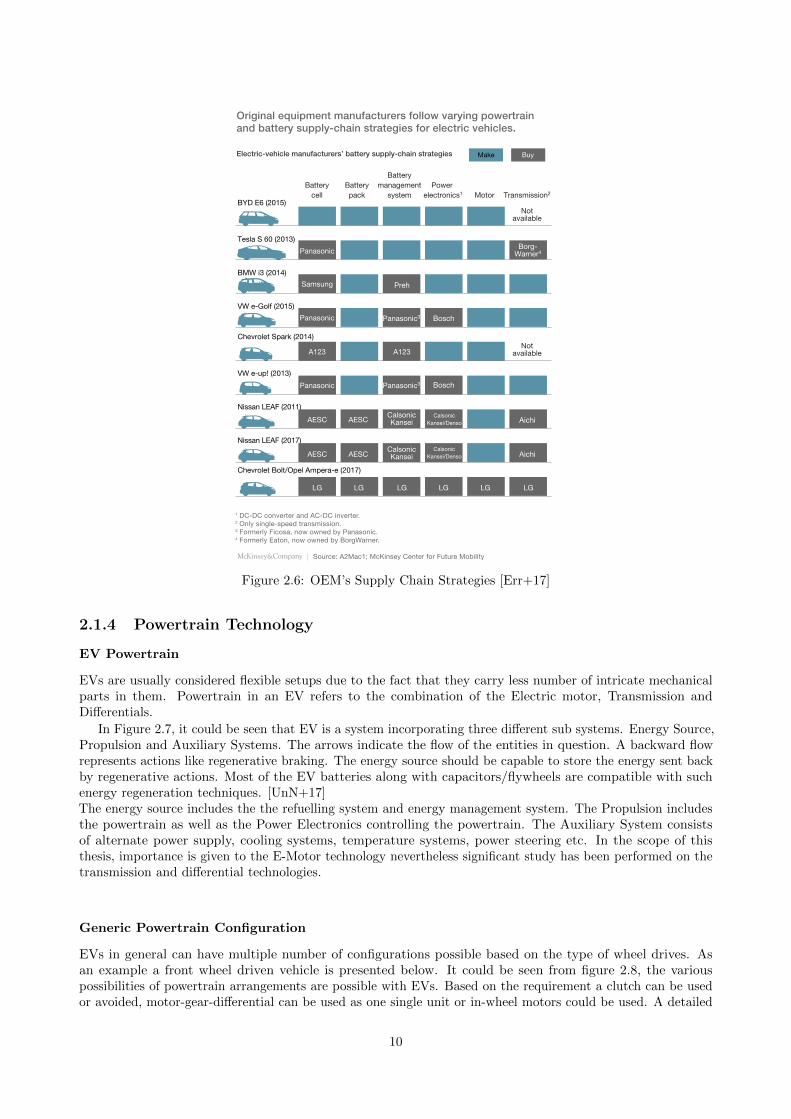
Figure 2.6: OEM’s Supply Chain Strategies [Err+17]

2.1.4 Powertrain Technology

EV Powertrain

EVs are usually considered flexible setups due to the fact that they carry less number of intricate mechanicalparts in them. Powertrain in an EV refers to the combination of the Electric motor, Transmission andDifferentials.

In Figure 2.7, it could be seen that EV is a system incorporating three different sub systems. Energy Source,Propulsion and Auxiliary Systems. The arrows indicate the flow of the entities in question. A backward flowrepresents actions like regenerative braking. The energy source should be capable to store the energy sent backby regenerative actions. Most of the EV batteries along with capacitors/flywheels are compatible with suchenergy regeneration techniques. [UnN+17]The energy source includes the the refuelling system and energy management system. The Propulsion includesthe powertrain as well as the Power Electronics controlling the powertrain. The Auxiliary System consistsof alternate power supply, cooling systems, temperature systems, power steering etc. In the scope of thisthesis, importance is given to the E-Motor technology nevertheless significant study has been performed on thetransmission and differential technologies.

Generic Powertrain Configuration

EVs in general can have multiple number of configurations possible based on the type of wheel drives. Asan example a front wheel driven vehicle is presented below. It could be seen from figure 2.8, the variouspossibilities of powertrain arrangements are possible with EVs. Based on the requirement a clutch can be usedor avoided, motor-gear-differential can be used as one single unit or in-wheel motors could be used. A detailed

10

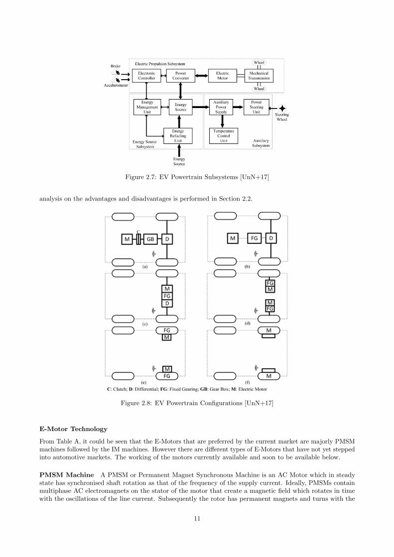
Figure 2.7: EV Powertrain Subsystems [UnN+17]

analysis on the advantages and disadvantages is performed in Section 2.2.

Figure 2.8: EV Powertrain Configurations [UnN+17]

E-Motor Technology

From Table A, it could be seen that the E-Motors that are preferred by the current market are majorly PMSMmachines followed by the IM machines. However there are different types of E-Motors that have not yet steppedinto automotive markets. The working of the motors currently available and soon to be available below.

PMSM Machine A PMSM or Permanent Magnet Synchronous Machine is an AC Motor which in steadystate has synchronised shaft rotation as that of the frequency of the supply current. Ideally, PMSMs containmultiphase AC electromagnets on the stator of the motor that create a magnetic field which rotates in timewith the oscillations of the line current. Subsequently the rotor has permanent magnets and turns with the

11

stator field in the same rate. This results in a second synchronised rotating magnetic field. For synchronousmotors the voltage equation can be given as equation 2.1. Equation 2.1 relates the d and q axis voltage (vd &vq) with d and q axis currents (id & iq),d and q axis inductance (Ld & Lq), motor angular speed (ωm),armatureflux linkages due to from permanent magnets along the d-q axis (ϕa),resistance of the stator windings (R) andnumber of pole pairs (p). [

vdvq

]=

[R+ pLd −ωmLq

ωmLd R+ pLq

] [idiq

]+

[0

ωmϕa

](2.1)

The output torque (T ) can be given by equation 2.2. In this equation the torque is a function of arma-ture current (Ia) and armature current lead angle from the q-axis (β)

T = p

{ϕaIacosβ +

1

2(Ld − Lq) I2asin2β

}(2.2)

Depending on the arrangements of the magnets, these motors are further divided into two broad categories.

SPMSM In this type of motor the arc-shaped magnets are mounted on the surface of the rotor core. Thesemagnets are also covered from outside with the help of steel sheets to avoid any magnet fallouts.Lack ofmagnetic saliency makes this motor use the magnetic torque alone. The maximum torque in this case isachieved at β=0 in equation 2.2. This is considered to be the most efficient phase angle. The motor having asimple construction has a major disadvantage of eddy current losses due to the steel coverings.

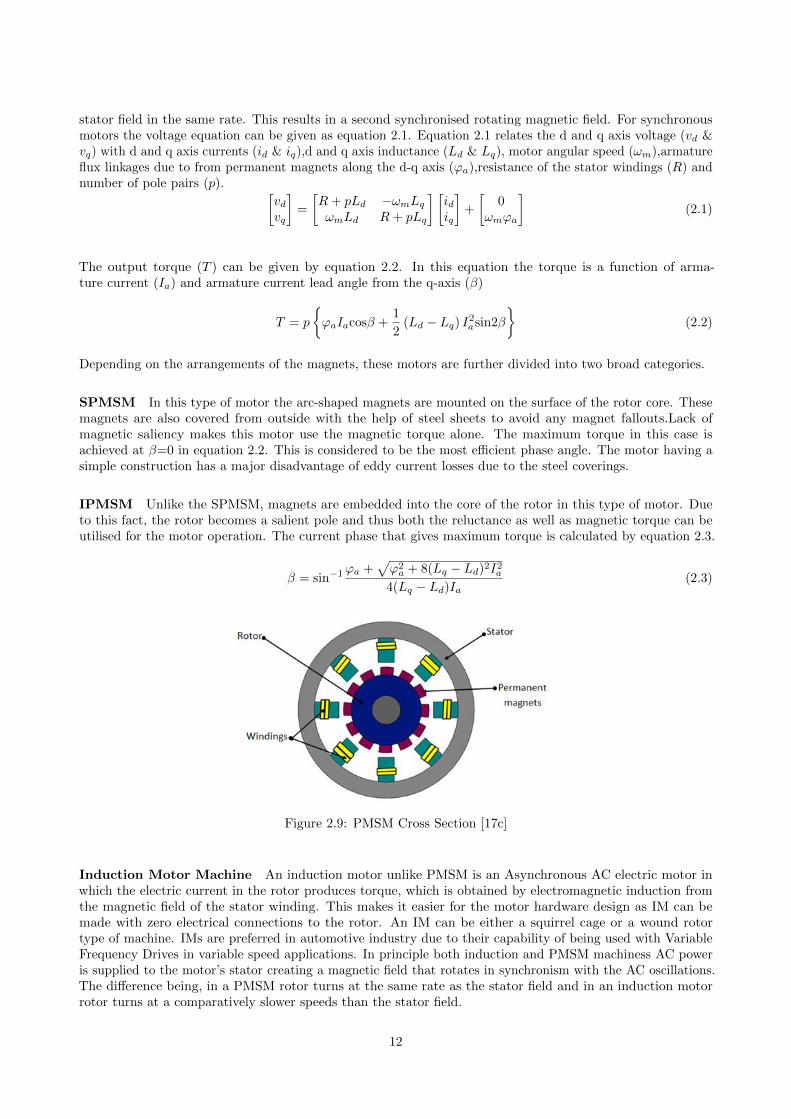
IPMSM Unlike the SPMSM, magnets are embedded into the core of the rotor in this type of motor. Dueto this fact, the rotor becomes a salient pole and thus both the reluctance as well as magnetic torque can beutilised for the motor operation. The current phase that gives maximum torque is calculated by equation 2.3.

β = sin−1ϕa +√ϕ2a + 8(Lq − Ld)2I2a

4(Lq − Ld)Ia(2.3)

Figure 2.9: PMSM Cross Section [17c]

Induction Motor Machine An induction motor unlike PMSM is an Asynchronous AC electric motor inwhich the electric current in the rotor produces torque, which is obtained by electromagnetic induction fromthe magnetic field of the stator winding. This makes it easier for the motor hardware design as IM can bemade with zero electrical connections to the rotor. An IM can be either a squirrel cage or a wound rotortype of machine. IMs are preferred in automotive industry due to their capability of being used with VariableFrequency Drives in variable speed applications. In principle both induction and PMSM machiness AC poweris supplied to the motor’s stator creating a magnetic field that rotates in synchronism with the AC oscillations.The difference being, in a PMSM rotor turns at the same rate as the stator field and in an induction motorrotor turns at a comparatively slower speeds than the stator field.

12

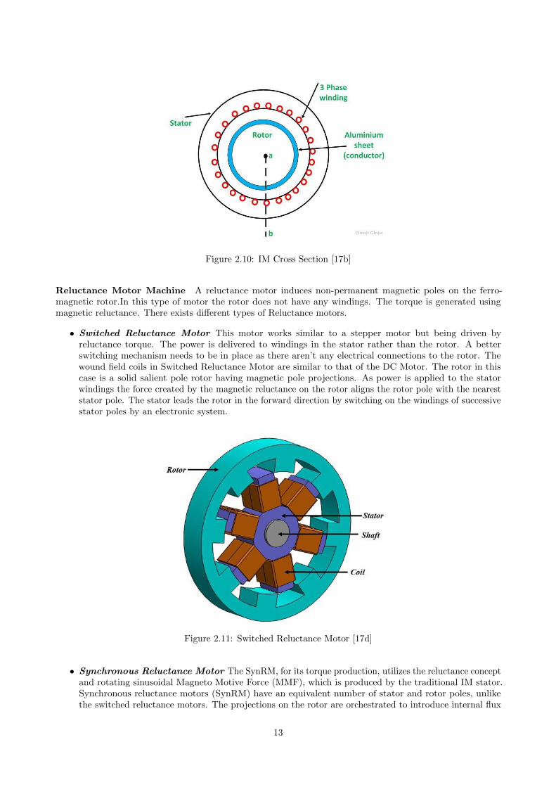
Figure 2.10: IM Cross Section [17b]

Reluctance Motor Machine A reluctance motor induces non-permanent magnetic poles on the ferro-magnetic rotor.In this type of motor the rotor does not have any windings. The torque is generated usingmagnetic reluctance. There exists different types of Reluctance motors.

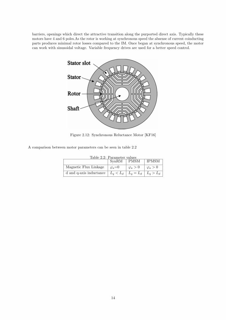
• Switched Reluctance Motor This motor works similar to a stepper motor but being driven byreluctance torque. The power is delivered to windings in the stator rather than the rotor. A betterswitching mechanism needs to be in place as there aren’t any electrical connections to the rotor. Thewound field coils in Switched Reluctance Motor are similar to that of the DC Motor. The rotor in thiscase is a solid salient pole rotor having magnetic pole projections. As power is applied to the statorwindings the force created by the magnetic reluctance on the rotor aligns the rotor pole with the neareststator pole. The stator leads the rotor in the forward direction by switching on the windings of successivestator poles by an electronic system.

Figure 2.11: Switched Reluctance Motor [17d]

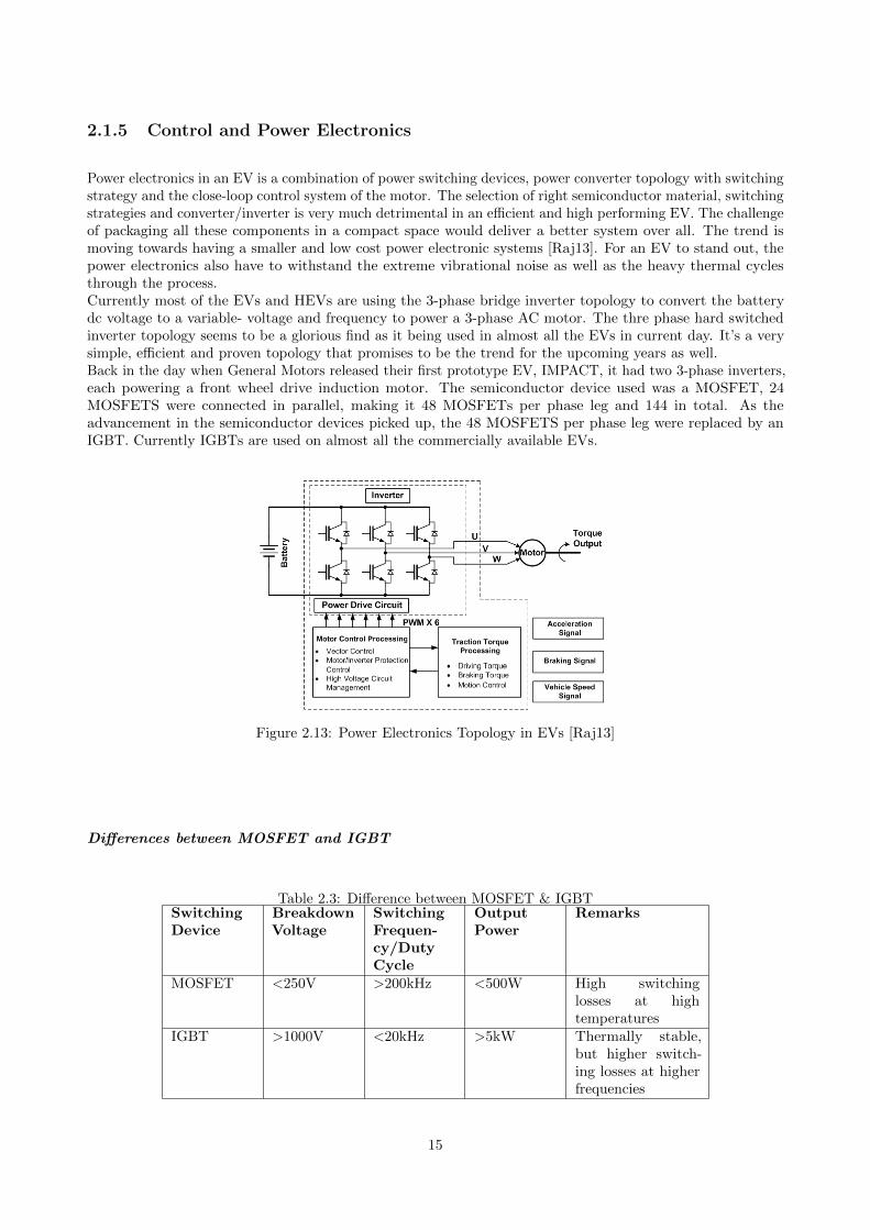
• Synchronous Reluctance Motor The SynRM, for its torque production, utilizes the reluctance conceptand rotating sinusoidal Magneto Motive Force (MMF), which is produced by the traditional IM stator.Synchronous reluctance motors (SynRM) have an equivalent number of stator and rotor poles, unlikethe switched reluctance motors. The projections on the rotor are orchestrated to introduce internal flux

13

barriers, openings which direct the attractive transition along the purported direct axis. Typically thesemotors have 4 and 6 poles.As the rotor is working at synchronous speed the absense of current coinductingparts produces minimal rotor losses compared to the IM. Once began at synchronous speed, the motorcan work with sinusoidal voltage. Variable frequency drives are used for a better speed control.

Figure 2.12: Synchronous Reluctance Motor [KF16]

A comparison between motor parameters can be seen in table 2.2

Table 2.2: Parameter valuesSynRM PMSM IPMSM

Magnetic Flux Linkage ϕa=0 ϕa > 0 ϕa > 0

d and q-axis inductance Lq < Ld Lq = Ld Lq > Ld

14

2.1.5 Control and Power Electronics

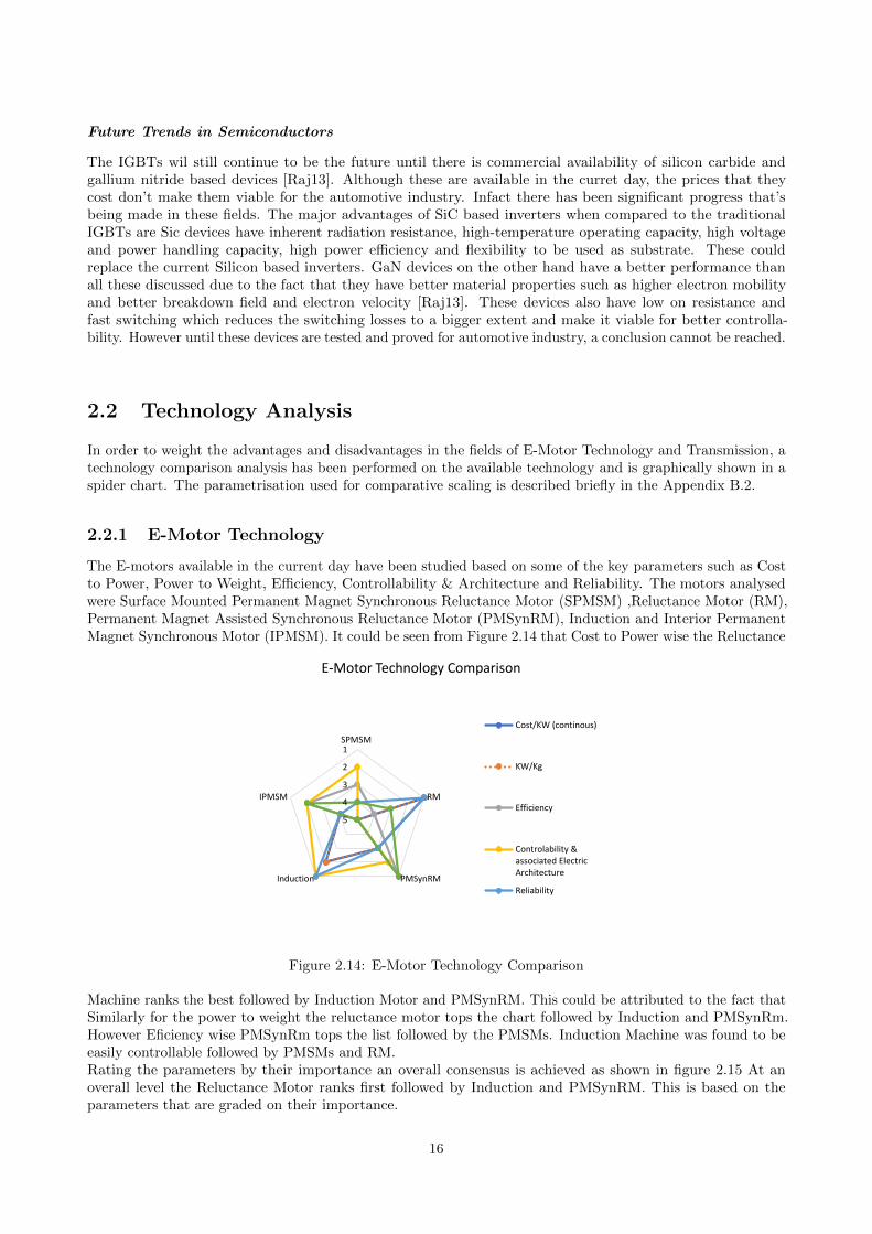
Power electronics in an EV is a combination of power switching devices, power converter topology with switchingstrategy and the close-loop control system of the motor. The selection of right semiconductor material, switchingstrategies and converter/inverter is very much detrimental in an efficient and high performing EV. The challengeof packaging all these components in a compact space would deliver a better system over all. The trend ismoving towards having a smaller and low cost power electronic systems [Raj13]. For an EV to stand out, thepower electronics also have to withstand the extreme vibrational noise as well as the heavy thermal cyclesthrough the process.Currently most of the EVs and HEVs are using the 3-phase bridge inverter topology to convert the batterydc voltage to a variable- voltage and frequency to power a 3-phase AC motor. The thre phase hard switchedinverter topology seems to be a glorious find as it being used in almost all the EVs in current day. It’s a verysimple, efficient and proven topology that promises to be the trend for the upcoming years as well.Back in the day when General Motors released their first prototype EV, IMPACT, it had two 3-phase inverters,each powering a front wheel drive induction motor. The semiconductor device used was a MOSFET, 24MOSFETS were connected in parallel, making it 48 MOSFETs per phase leg and 144 in total. As theadvancement in the semiconductor devices picked up, the 48 MOSFETS per phase leg were replaced by anIGBT. Currently IGBTs are used on almost all the commercially available EVs.

Figure 2.13: Power Electronics Topology in EVs [Raj13]

Differences between MOSFET and IGBT

Table 2.3: Difference between MOSFET & IGBTSwitchingDevice

BreakdownVoltage

SwitchingFrequen-cy/DutyCycle

OutputPower

Remarks

MOSFET <250V >200kHz <500W High switchinglosses at hightemperatures

IGBT >1000V <20kHz >5kW Thermally stable,but higher switch-ing losses at higherfrequencies

15

Future Trends in Semiconductors

The IGBTs wil still continue to be the future until there is commercial availability of silicon carbide andgallium nitride based devices [Raj13]. Although these are available in the curret day, the prices that theycost don’t make them viable for the automotive industry. Infact there has been significant progress that’sbeing made in these fields. The major advantages of SiC based inverters when compared to the traditionalIGBTs are Sic devices have inherent radiation resistance, high-temperature operating capacity, high voltageand power handling capacity, high power efficiency and flexibility to be used as substrate. These couldreplace the current Silicon based inverters. GaN devices on the other hand have a better performance thanall these discussed due to the fact that they have better material properties such as higher electron mobilityand better breakdown field and electron velocity [Raj13]. These devices also have low on resistance andfast switching which reduces the switching losses to a bigger extent and make it viable for better controlla-bility. However until these devices are tested and proved for automotive industry, a conclusion cannot be reached.

2.2 Technology Analysis

In order to weight the advantages and disadvantages in the fields of E-Motor Technology and Transmission, atechnology comparison analysis has been performed on the available technology and is graphically shown in aspider chart. The parametrisation used for comparative scaling is described briefly in the Appendix B.2.

2.2.1 E-Motor Technology

The E-motors available in the current day have been studied based on some of the key parameters such as Costto Power, Power to Weight, Efficiency, Controllability & Architecture and Reliability. The motors analysedwere Surface Mounted Permanent Magnet Synchronous Reluctance Motor (SPMSM) ,Reluctance Motor (RM),Permanent Magnet Assisted Synchronous Reluctance Motor (PMSynRM), Induction and Interior PermanentMagnet Synchronous Motor (IPMSM). It could be seen from Figure 2.14 that Cost to Power wise the Reluctance

1

2

3

4

5

SPMSM

RM

PMSynRMInduction

IPMSM

E-Motor Technology Comparison

Cost/KW (continous)

KW/Kg

Efficiency

Controlability &associated ElectricArchitecture

Reliability

Figure 2.14: E-Motor Technology Comparison

Machine ranks the best followed by Induction Motor and PMSynRM. This could be attributed to the fact thatSimilarly for the power to weight the reluctance motor tops the chart followed by Induction and PMSynRm.However Eficiency wise PMSynRm tops the list followed by the PMSMs. Induction Machine was found to beeasily controllable followed by PMSMs and RM.Rating the parameters by their importance an overall consensus is achieved as shown in figure 2.15 At anoverall level the Reluctance Motor ranks first followed by Induction and PMSynRM. This is based on theparameters that are graded on their importance.

16

1

1.5

2

2.5

3

3.5

4

4.5

5

SPMSM

RM

PMSynRMInduction

IPMSM

E-Motor Technology Overall Rank

Figure 2.15: E-Motor Technology Overall Comparison

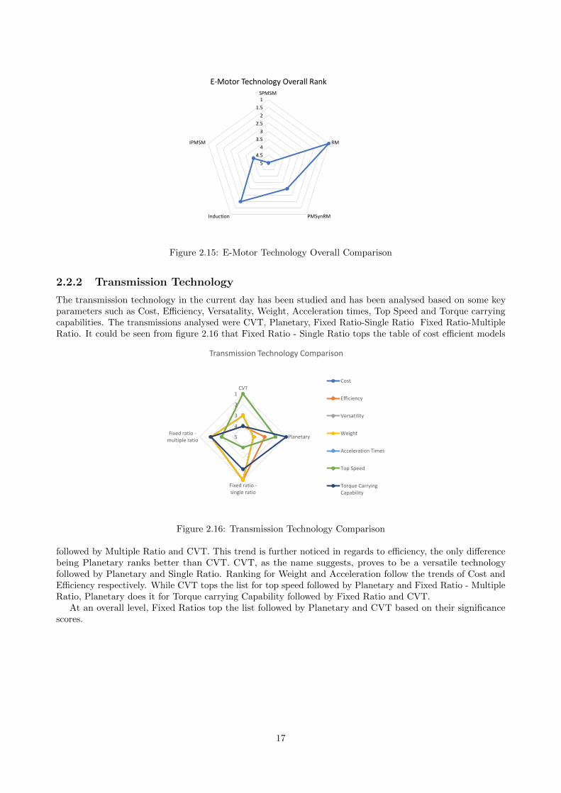
2.2.2 Transmission Technology

The transmission technology in the current day has been studied and has been analysed based on some keyparameters such as Cost, Efficiency, Versatality, Weight, Acceleration times, Top Speed and Torque carryingcapabilities. The transmissions analysed were CVT, Planetary, Fixed Ratio-Single Ratio Fixed Ratio-MultipleRatio. It could be seen from figure 2.16 that Fixed Ratio - Single Ratio tops the table of cost efficient models

1

2

3

4

5

CVT

Planetary

Fixed ratio -single ratio

Fixed ratio -multiple ratio

Transmission Technology Comparison

Cost

Efficiency

Versatility

Weight

Acceleration Times

Top Speed

Torque CarryingCapability

Figure 2.16: Transmission Technology Comparison

followed by Multiple Ratio and CVT. This trend is further noticed in regards to efficiency, the only differencebeing Planetary ranks better than CVT. CVT, as the name suggests, proves to be a versatile technologyfollowed by Planetary and Single Ratio. Ranking for Weight and Acceleration follow the trends of Cost andEfficiency respectively. While CVT tops the list for top speed followed by Planetary and Fixed Ratio - MultipleRatio, Planetary does it for Torque carrying Capability followed by Fixed Ratio and CVT.

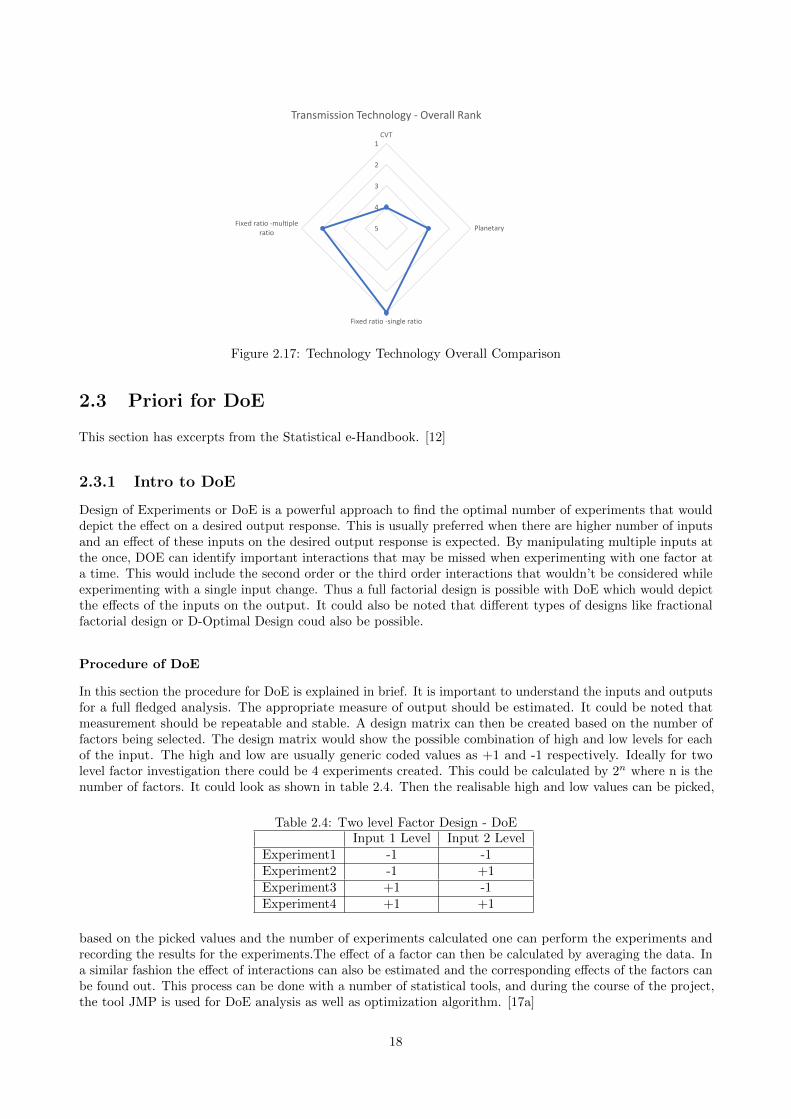
At an overall level, Fixed Ratios top the list followed by Planetary and CVT based on their significancescores.

17

1

2

3

4

5

CVT

Planetary

Fixed ratio -single ratio

Fixed ratio -multipleratio

Transmission Technology - Overall Rank

Figure 2.17: Technology Technology Overall Comparison

2.3 Priori for DoE

This section has excerpts from the Statistical e-Handbook. [12]

2.3.1 Intro to DoE

Design of Experiments or DoE is a powerful approach to find the optimal number of experiments that woulddepict the effect on a desired output response. This is usually preferred when there are higher number of inputsand an effect of these inputs on the desired output response is expected. By manipulating multiple inputs atthe once, DOE can identify important interactions that may be missed when experimenting with one factor ata time. This would include the second order or the third order interactions that wouldn’t be considered whileexperimenting with a single input change. Thus a full factorial design is possible with DoE which would depictthe effects of the inputs on the output. It could also be noted that different types of designs like fractionalfactorial design or D-Optimal Design coud also be possible.

Procedure of DoE

In this section the procedure for DoE is explained in brief. It is important to understand the inputs and outputsfor a full fledged analysis. The appropriate measure of output should be estimated. It could be noted thatmeasurement should be repeatable and stable. A design matrix can then be created based on the number offactors being selected. The design matrix would show the possible combination of high and low levels for eachof the input. The high and low are usually generic coded values as +1 and -1 respectively. Ideally for twolevel factor investigation there could be 4 experiments created. This could be calculated by 2n where n is thenumber of factors. It could look as shown in table 2.4. Then the realisable high and low values can be picked,

Table 2.4: Two level Factor Design - DoEInput 1 Level Input 2 Level

Experiment1 -1 -1Experiment2 -1 +1Experiment3 +1 -1Experiment4 +1 +1

based on the picked values and the number of experiments calculated one can perform the experiments andrecording the results for the experiments.The effect of a factor can then be calculated by averaging the data. Ina similar fashion the effect of interactions can also be estimated and the corresponding effects of the factors canbe found out. This process can be done with a number of statistical tools, and during the course of the project,the tool JMP is used for DoE analysis as well as optimization algorithm. [17a]

18

2.3.2 Adopted Experimental Design Setup

In this thesis, a D-Optimal design is performed and the classical designs like the factorial and fraction factorialdesign are not considered due to the fact that the latter design matrices are orthogonal and effect estimates arenot correlated. In a D-Optimal design orthogonal design matrices are possible and the effect estimates can becorrelated. However the interaction designs can still be performed with this design. The two major reasons forusing a D-Optimal design are,

• Classical designs like factorial or fractional factorial need a lot of runs for the amount of resources ortime allowed for the experiments

• The design is constrained

Thus when the design has to be constrained, which is the case in this thesis, a D-Optimal Design is favoured.

2.3.3 Model Fitting & Optimisation

Model Fitting

One of the major points in model building is the model validation. One could easily identify if the modelfits right with the value of variance. A higher R2 value ususally signifies a better fit. However this isn’t theonly way to validate the model. A graphical residual analysis gives a better picture of how well the model fits.Alongside the R2 statistic a graphical analysis would readily illustrate a broad range of complex aspects of therelationship between the model and the data. The residuals are the differences between the observed valueof the combination of inputs and the corresponding prediction of the response computed by a regression analysis.

Optimisation

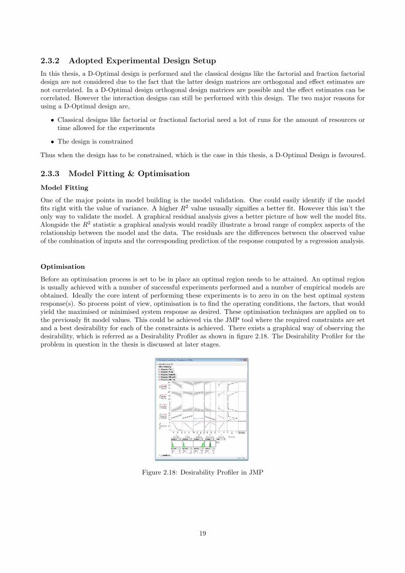
Before an optimisation process is set to be in place an optimal region needs to be attained. An optimal regionis usually achieved with a number of successful experiments performed and a number of empirical models areobtained. Ideally the core intent of performing these experiments is to zero in on the best optimal systemresponse(s). So process point of view, optimisation is to find the operating conditions, the factors, that wouldyield the maximised or minimised system response as desired. These optimisation techniques are applied on tothe previously fit model values. This could be achieved via the JMP tool where the required constraints are setand a best desirability for each of the constraints is achieved. There exists a graphical way of observing thedesirability, which is referred as a Desirability Profiler as shown in figure 2.18. The Desirability Profiler for theproblem in question in the thesis is discussed at later stages.

Figure 2.18: Desirability Profiler in JMP

19

20

3 Selection of Use Cases

This chapter describes the procedure and rational for the selection of use cases upon which the performanceof the drive-trains is compared. A total of three use cases are identified keeping in mind the scope of thethesis,these are described below.

3.1 Cruise Control

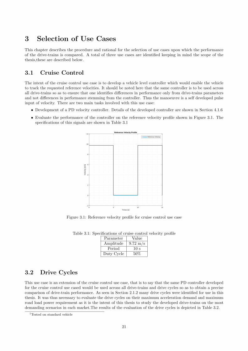
The intent of the cruise control use case is to develop a vehicle level controller which would enable the vehicleto track the requested reference velocities. It should be noted here that the same controller is to be used acrossall drive-trains so as to ensure that one identifies differences in performance only from drive-trains parametersand not differences in performance stemming from the controller. Thus the manoeuvre is a self developed pulseinput of velocity. There are two main tasks involved with this use case:

• Development of a PD velocity controller. Details of the developed controller are shown in Section 4.1.6

• Evaluate the performance of the controller on the reference velocity profile shown in Figure 3.1. Thespecifications of this signals are shown in Table 3.1

0 5 10 15

Times [s]

-2

0

2

4

6

8

10

12

Vel

ocity

[m/s

]

Reference Velocity Profile

Reference Velocity

Figure 3.1: Reference velocity profile for cruise control use case

Table 3.1: Specifications of cruise control velocity profileParameter ValueAmplitude 9.72 m/s

Period 10 sDuty Cycle 50%

3.2 Drive Cycles

This use case is an extension of the cruise control use case, that is to say that the same PD controller developedfor the cruise control use cased would be used across all drive-trains and drive cycles so as to obtain a precisecomparison of drive-train performance. As seen in Section 2.1.2 many drive cycles were identified for use in thisthesis. It was thus necessary to evaluate the drive cycles on their maximum acceleration demand and maximumroad load power requirement as it is the intent of this thesis to study the developed drive-trains on the mostdemanding scenarios in each market.The results of the evaluation of the drive cycles is depicted in Table 3.2.

1Tested on standard vehicle

21

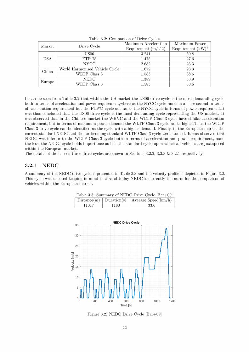
Table 3.2: Comparison of Drive Cycles

Market Drive CycleMaximum AccelerationRequirement (m/sˆ2)

Maximum PowerRequirement (kW)1

USAUS06 3.241 59.8

FTP 75 1.475 27.6NYCC 2.682 23.3

ChinaWorld Harmonised Vehicle Cycle 1.672 23.3

WLTP Class 3 1.583 38.6

EuropeNEDC 1.389 33.9

WLTP Class 3 1.583 38.6

It can be seen from Table 3.2 that within the US market the US06 drive cycle is the most demanding cycleboth in terms of acceleration and power requirement,where as the NYCC cycle ranks in a close second in termsof acceleration requirement but the FTP75 cycle out ranks the NYCC cycle in terms of power requirement.Itwas thus concluded that the US06 drive-cycle is the most demanding cycle representing the US market. Itwas observed that in the Chinese market the WHVC and the WLTP Class 3 cycle have similar accelerationrequirement, but in terms of maximum power demand the WLTP Class 3 cycle ranks higher.Thus the WLTPClass 3 drive cycle can be identified as the cycle with a higher demand. Finally, in the European market thecurrent standard NEDC and the forthcoming standard WLTP Class 3 cycle were studied. It was observed thatNEDC was inferior to the WLTP Class 3 cycle both in terms of acceleration and power requirement, nonethe less, the NEDC cycle holds importance as it is the standard cycle upon which all vehicles are juxtaposedwithin the European market.The details of the chosen three drive cycles are shown in Sections 3.2.2, 3.2.3 & 3.2.1 respectively.

3.2.1 NEDC

A summary of the NEDC drive cycle is presented in Table 3.3 and the velocity profile is depicted in Figure 3.2.This cycle was selected keeping in mind that as of today NEDC is currently the norm for the comparison ofvehicles within the European market.

Table 3.3: Summary of NEDC Drive Cycle [Bar+09]Distance(m) Duration(s) Average Speed(km/h)

11017 1180 33.6

0 200 400 600 800 1000 1200

Time [s]

0

5

10

15

20

25

30

35

Vel

ocity

[m/s

]

NEDC Drive Cycle

Figure 3.2: NEDC Drive Cycle [Bar+09]

22

3.2.2 US06

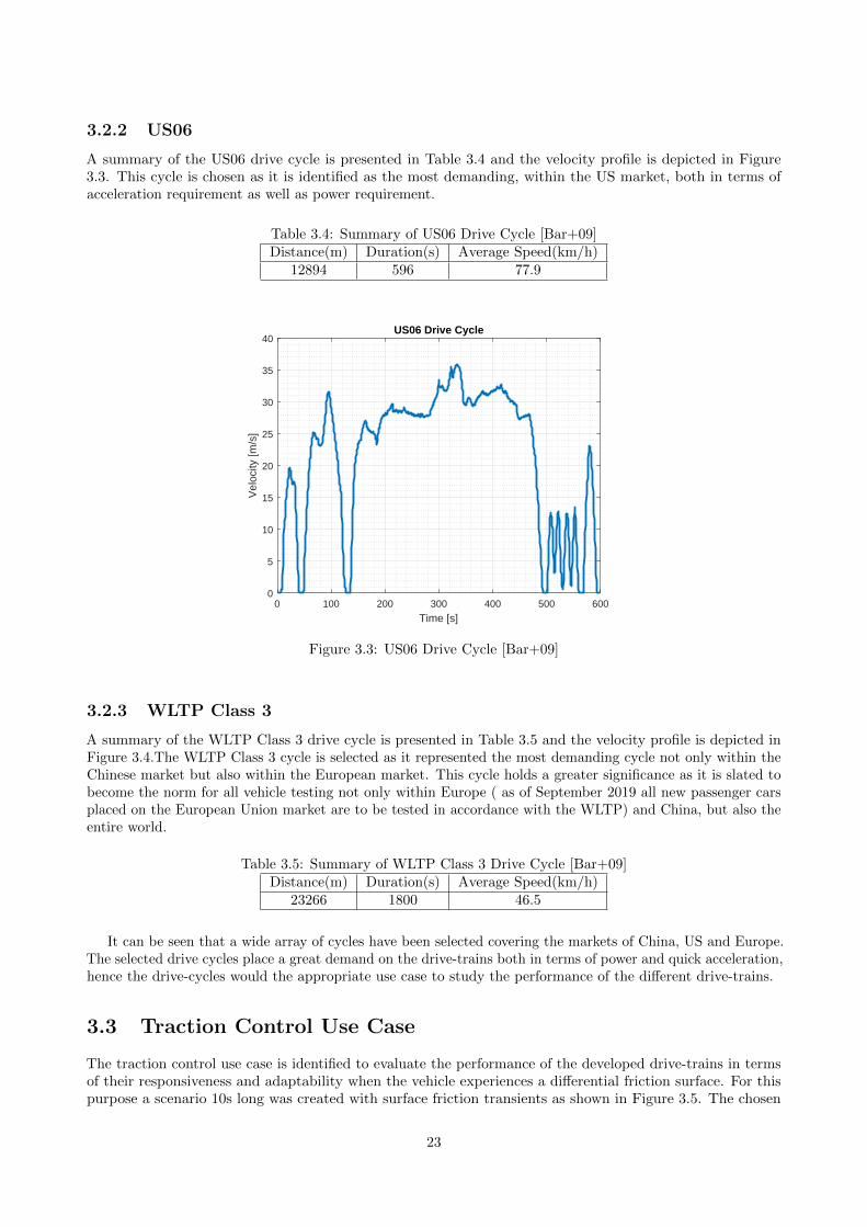
A summary of the US06 drive cycle is presented in Table 3.4 and the velocity profile is depicted in Figure3.3. This cycle is chosen as it is identified as the most demanding, within the US market, both in terms ofacceleration requirement as well as power requirement.

Table 3.4: Summary of US06 Drive Cycle [Bar+09]Distance(m) Duration(s) Average Speed(km/h)

12894 596 77.9

0 100 200 300 400 500 600

Time [s]

0

5

10

15

20

25

30

35

40

Vel

ocity

[m/s

]

US06 Drive Cycle

Figure 3.3: US06 Drive Cycle [Bar+09]

3.2.3 WLTP Class 3

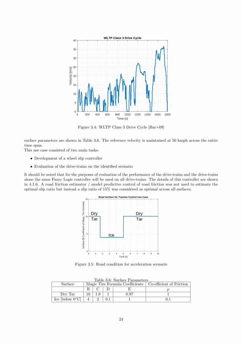
A summary of the WLTP Class 3 drive cycle is presented in Table 3.5 and the velocity profile is depicted inFigure 3.4.The WLTP Class 3 cycle is selected as it represented the most demanding cycle not only within theChinese market but also within the European market. This cycle holds a greater significance as it is slated tobecome the norm for all vehicle testing not only within Europe ( as of September 2019 all new passenger carsplaced on the European Union market are to be tested in accordance with the WLTP) and China, but also theentire world.

Table 3.5: Summary of WLTP Class 3 Drive Cycle [Bar+09]Distance(m) Duration(s) Average Speed(km/h)

23266 1800 46.5

It can be seen that a wide array of cycles have been selected covering the markets of China, US and Europe.The selected drive cycles place a great demand on the drive-trains both in terms of power and quick acceleration,hence the drive-cycles would the appropriate use case to study the performance of the different drive-trains.

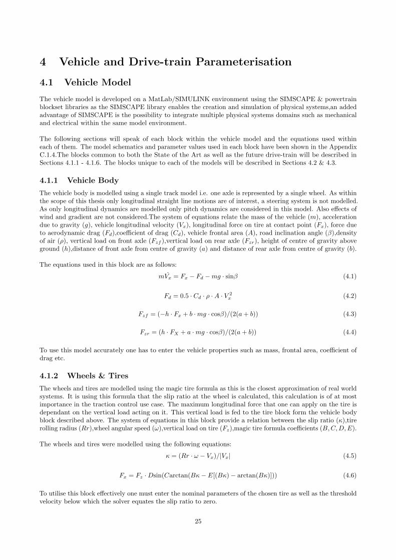
3.3 Traction Control Use Case

The traction control use case is identified to evaluate the performance of the developed drive-trains in termsof their responsiveness and adaptability when the vehicle experiences a differential friction surface. For thispurpose a scenario 10s long was created with surface friction transients as shown in Figure 3.5. The chosen

23

0 200 400 600 800 1000 1200 1400 1600 1800

Time [s]

0

5

10

15

20

25

30

35

40

Vel

ocity

[m/s

]

WLTP Class 3 Drive Cycle

Figure 3.4: WLTP Class 3 Drive Cycle [Bar+09]

surface parameters are shown in Table 3.6. The reference velocity is maintained at 50 kmph across the entiretime span.This use case consisted of two main tasks:

• Development of a wheel slip controller

• Evaluation of the drive-trains on the identified scenario

It should be noted that for the purposes of evaluation of the performance of the drive-trains and the drive-trainsalone the same Fuzzy Logic controller will be used on all drive-trains. The details of this controller are shownin 4.1.6. A road friction estimator / model predictive control of road friction was not used to estimate theoptimal slip ratio but instead a slip ratio of 15% was considered as optimal across all surfaces.

0 1 2 3 4 5 6 7 8 9 10

Time [s]

0

5

10

15

Sur

face

[B C

oeffi

cien

t of M

agic

Tire

For

mul

a]

Road Surface for Traction Control Use Case

DryTar

DryTar

Ice

Figure 3.5: Road condition for acceleration scenario

Table 3.6: Surface ParametersSurface Magic Tire Formula Coefficients Co-efficient of Friction

B C D E µDry Tar 10 1.9 1 0.97 1

Ice [below 0◦C] 4 2 0.1 1 0.1

24

4 Vehicle and Drive-train Parameterisation

4.1 Vehicle Model

The vehicle model is developed on a MatLab/SIMULINK environment using the SIMSCAPE & powertrainblockset libraries as the SIMSCAPE library enables the creation and simulation of physical systems,an addedadvantage of SIMSCAPE is the possibility to integrate multiple physical systems domains such as mechanicaland electrical within the same model environment.

The following sections will speak of each block within the vehicle model and the equations used withineach of them. The model schematics and parameter values used in each block have been shown in the AppendixC.1.4.The blocks common to both the State of the Art as well as the future drive-train will be described inSections 4.1.1 - 4.1.6. The blocks unique to each of the models will be described in Sections 4.2 & 4.3.

4.1.1 Vehicle Body

The vehicle body is modelled using a single track model i.e. one axle is represented by a single wheel. As withinthe scope of this thesis only longitudinal straight line motions are of interest, a steering system is not modelled.As only longitudinal dynamics are modelled only pitch dynamics are considered in this model. Also effects ofwind and gradient are not considered.The system of equations relate the mass of the vehicle (m), accelerationdue to gravity (g), vehicle longitudinal velocity (Vx), longitudinal force on tire at contact point (Fx), force dueto aerodynamic drag (Fd),coefficient of drag (Cd), vehicle frontal area (A), road inclination angle (β),densityof air (ρ), vertical load on front axle (Fzf ),vertical load on rear axle (Fzr), height of centre of gravity aboveground (h),distance of front axle from centre of gravity (a) and distance of rear axle from centre of gravity (b).

The equations used in this block are as follows:

mVx = Fx − Fd −mg · sinβ (4.1)

Fd = 0.5 · Cd · ρ ·A · V 2x (4.2)

Fzf = (−h · Fx + b ·mg · cosβ)/(2(a+ b)) (4.3)

Fzr = (h · FX + a ·mg · cosβ)/(2(a+ b)) (4.4)

To use this model accurately one has to enter the vehicle properties such as mass, frontal area, coefficient ofdrag etc.

4.1.2 Wheels & Tires

The wheels and tires are modelled using the magic tire formula as this is the closest approximation of real worldsystems. It is using this formula that the slip ratio at the wheel is calculated, this calculation is of at mostimportance in the traction control use case. The maximum longitudinal force that one can apply on the tire isdependant on the vertical load acting on it. This vertical load is fed to the tire block form the vehicle bodyblock described above. The system of equations in this block provide a relation between the slip ratio (κ),tirerolling radius (Rr),wheel angular speed (ω),vertical load on tire (Fz),magic tire formula coefficients (B,C,D,E).

The wheels and tires were modelled using the following equations:

κ = (Rr · ω − Vx)/|Vx| (4.5)

Fx = Fz ·Dsin(Carctan(Bκ− E[(Bκ)− arctan(Bκ)])) (4.6)

To utilise this block effectively one must enter the nominal parameters of the chosen tire as well as the thresholdvelocity below which the solver equates the slip ratio to zero.

25

4.1.3 Transmission

To model the transmission a simple gearbox is utilised. The gearbox is modelled with two gear wheels a basegear wheel and the follower gear wheel. The base gear wheel is the one which is attached to the motor andthe follower gear wheel is the one connected to the differential. Due to limitations within the gear box modelThe inertia of the gear wheels are not present within the gear box but are connected as an external inertia. Itshould be noted here that the inertia of the base and follower gear wheels have been calculated based onlyon their radii and are independent of their masses.The system of equations in this block relate the gear ratio(N),radius of follower gear (rf ),radius of base gear (rb),torque acting on base gear (τb),torque acting on followergear (τf ),losses in torque transfer calculated based on the efficiency parameter (τloss),follower gear angularvelocity (ωf ),base gear angular velocity (ωb),follower gear inertia (Jf ) ,base gear inertia (Jb).

The equations used in the modelling of the gearbox are as follows:

N = rf/rb (4.7)

Nτb + τf − τloss = 0 (4.8)

τb = Jb · ωb (4.9)

τf = Jf · ωf (4.10)

To utilise this model effectively one must provide parameters such as efficiency, damping and gear ratio.

4.1.4 Open Differential

The open differential is modelled using an arrangement of a single simple gearbox along with two Sun-Planetbevel gears. The output shafts of the two Sun-planet bevel gears are connected to each of the wheels. Theinput shaft to each of the bevel gears comes form the simple gearbox. This gear box is fed torque from thetransmission system described in Section 4.1.3.To utilise this block effectively one must provide the final driveratio, inertia of the input shaft/gear arrangement and inertia of the two output gear/shaft arrangement. Theequations used in this block are similar to those used in Section 4.1.3

4.1.5 Battery

A simple battery model is used as a part of this thesis as modelling the battery with discharge dynamics, finitecharge and non-ideal resistances in beyond the scope of this thesis. The battery is modelled as a constantvoltage source of infinite energy, this voltage source is capable of maintaining the required potential irrespectiveof the current drawn from the battery.

4.1.6 Vehicle Controllers

In this section the developed cruise controller as well as the traction controller will be discussed.

Velocity Controller(Cruise Control)

The velocity controller developed for the cruise control and drive cycle use case is a PD controller. A PDcontroller is deemed as the optimal controller configuration as the velocity and acceleration of the vehicle areto be controlled and not its position. It can also be understood that the addition of the differential gain andremoval of the integral gain tends to decrease the overshoot and the settling time whilst marginally improvingthe stability of the system. The only draw back is that the derivative system is highly sensitive to noise,this isnot a cause of concern within the scope of this thesis as no noise models have been introduced,i.e. a completelydeterministic system is studied.

The controller accepts an input of error (formulated in Equation 4.11) and outputs a control signal. The

26

control signal has values between -1 and 1, wherein 1 denotes maximum acceleration (complete depressionof accelerator pedal) and -1 denotes maximum braking (complete depression of brake pedal), any positivevalues(between 0 and 1) represents partial depression of the accelerator pedal and any negative value (between-1 and 0) represents partial depression of the brake pedal.This logic is represented in Equation 4.12 whereVreference is the reference/target velocity for the vehicle.

error = Vreference − Vx (4.11)

ControllerOutput =

1 : MaximumAcceleration(0, 1) : PartialAcceleration0 : NoOperation(−1, 0) : PartialDeceleration−1 : MaximumDeceleration

(4.12)

Furthermore, the tuning of the controller was carried out by studying the linearised plant system at differentoperating points.The transfer function of the plant at various operating points is shown in Table C.5 Havingidentified the plant dynamics one can derive the transfer function of the PD controller as in Equation 4.13.The tuned proportional (P ) and derivative (D) gains of the controller are presented in the appendix.

TransferFunction = P +Ds/(s+ 1) (4.13)

Traction Controller

In this section the traction controller designed to limit wheel slip will be described. To select the type ofcontroller a review of existing literature is carried out from the review of existing literature it is observed thatthe Fuzzy Logic type of control had the greatest potential in Traction control applications as stated in [Zet07].[Zet07] also states that ”The fuzzy controller, however, performed very well in all the tests. Besides frombeing nonlinear, it does not need a desired value and manages to localise the peak of the -slip curve by itself.Furthermore, the fuzzy logic, upon which the controller is based, is very easy to understand.”, hence it wasdecided to implement a fuzzy logic controller.

The fuzzy logic controller accepts two inputs:

1. Vehicle Velocity Error

2. Wheel Slip Ratio Error

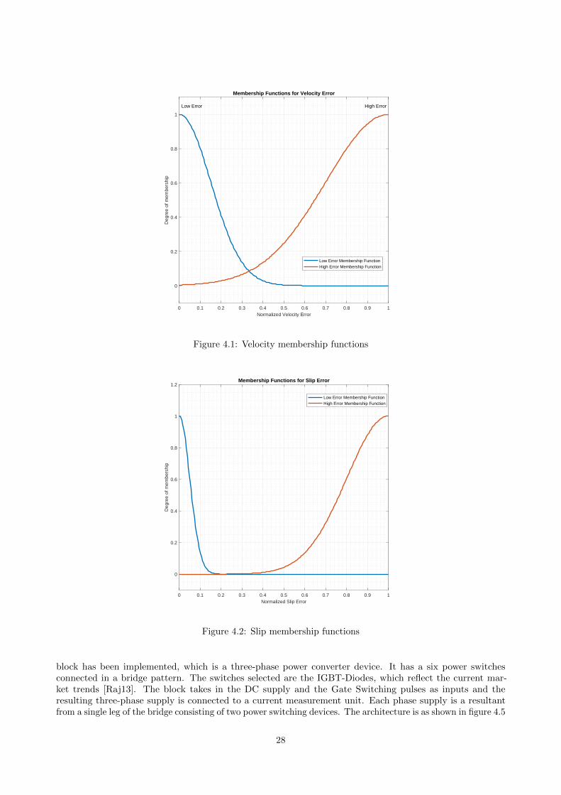
The vehicle velocity error is calculated by determining the deviation of the vehicle velocity from the referencevelocity(represented in Equation 4.11). The slip error is calculated by determining the deviation of the tire’sslip ratio from the optimal slip ratio which is assumed to be 15% for all surfaces. It is with these error inputsthat the controller determines if an accelerating or braking torque has to be applied on the wheel. In the casethat acceleration torque has to be applied the controller outputs a signal between 0 and 1 with 1 denotingmaximum acceleration and in the case of braking the controller outputs a signal between -1 and 0 with -1denoting maximum regenerative braking. The operation of the controller in the acceleration scenario is detailedbelow, the operation of the controller in the braking scenario is similar to that of the acceleration scenario, theonly difference being the controller output membership function. The output membership function for thebraking scenario is shown in Figure 4.3.

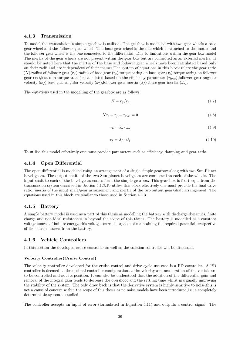
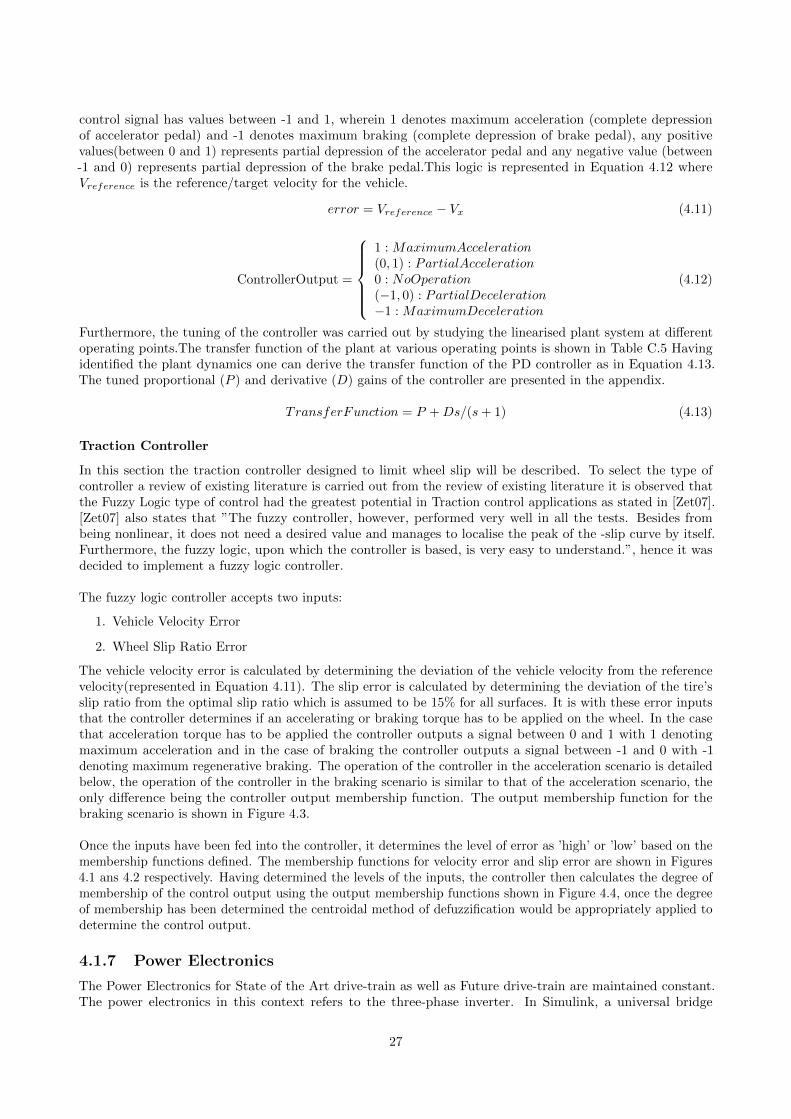
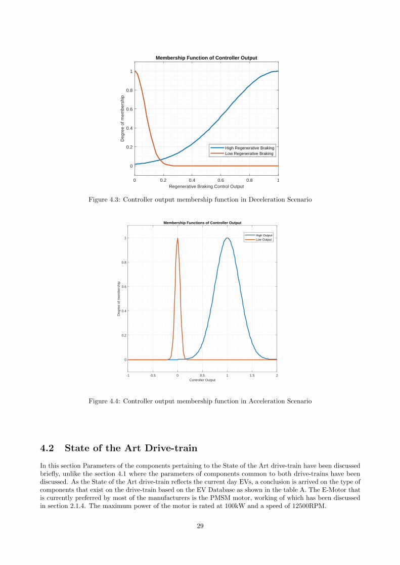
Once the inputs have been fed into the controller, it determines the level of error as ’high’ or ’low’ based on themembership functions defined. The membership functions for velocity error and slip error are shown in Figures4.1 ans 4.2 respectively. Having determined the levels of the inputs, the controller then calculates the degree ofmembership of the control output using the output membership functions shown in Figure 4.4, once the degreeof membership has been determined the centroidal method of defuzzification would be appropriately applied todetermine the control output.

4.1.7 Power Electronics

The Power Electronics for State of the Art drive-train as well as Future drive-train are maintained constant.The power electronics in this context refers to the three-phase inverter. In Simulink, a universal bridge

27

0 0.1 0.2 0.3 0.4 0.5 0.6 0.7 0.8 0.9 1Normalized Velocity Error

0

0.2

0.4

0.6

0.8

1

Deg

ree

of m

embe

rshi

p

Membership Functions for Velocity Error

Low Error High Error

Low Error Membership FunctionHigh Error Membership Function

Figure 4.1: Velocity membership functions

0 0.1 0.2 0.3 0.4 0.5 0.6 0.7 0.8 0.9 1Normalized Slip Error

0

0.2

0.4

0.6

0.8

1

1.2

Deg

ree

of m

embe

rshi

p

Membership Functions for Slip Error

Low Error Membership FunctionHigh Error Membership Function

Figure 4.2: Slip membership functions

block has been implemented, which is a three-phase power converter device. It has a six power switchesconnected in a bridge pattern. The switches selected are the IGBT-Diodes, which reflect the current mar-ket trends [Raj13]. The block takes in the DC supply and the Gate Switching pulses as inputs and theresulting three-phase supply is connected to a current measurement unit. Each phase supply is a resultantfrom a single leg of the bridge consisting of two power switching devices. The architecture is as shown in figure 4.5

28

0 0.2 0.4 0.6 0.8 1Regenerative Braking Control Output

0

0.2

0.4

0.6

0.8

1

Deg

ree

of m

embe

rshi

p

Membership Function of Controller Output

High Regenerative BrakingLow Regenerative Braking

Figure 4.3: Controller output membership function in Deceleration Scenario

-1 -0.5 0 0.5 1 1.5 2Controller Output

0

0.2

0.4

0.6

0.8

1

Deg

ree

of m

embe

rshi

p

Membership Functions of Controller Output

High OutputLow Output

Figure 4.4: Controller output membership function in Acceleration Scenario

4.2 State of the Art Drive-train

In this section Parameters of the components pertaining to the State of the Art drive-train have been discussedbriefly, unlike the section 4.1 where the parameters of components common to both drive-trains have beendiscussed. As the State of the Art drive-train reflects the current day EVs, a conclusion is arrived on the type ofcomponents that exist on the drive-train based on the EV Database as shown in the table A. The E-Motor thatis currently preferred by most of the manufacturers is the PMSM motor, working of which has been discussedin section 2.1.4. The maximum power of the motor is rated at 100kW and a speed of 12500RPM.

29

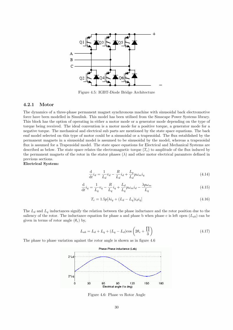
Figure 4.5: IGBT-Diode Bridge Architecture

4.2.1 Motor

The dynamics of a three-phase permanent magnet synchronous machine with sinusoidal back electromotiveforce have been modelled in Simulink. This model has been utilised from the Simscape Power Systems library.This block has the option of operating in either a motor mode or a generator mode depending on the type oftorque being received. The ideal convention is a motor mode for a positive torque, a generator mode for anegative torque. The mechanical and electrical sub parts are mentioned by the state space equations. The backemf model selected on this type of motor could be a sinusoidal or a trapezoidal. The flux established by thepermanent magnets in a sinusoidal model is assumed to be sinusoidal by the model, whereas a trapezoidalflux is assumed for a Trapezoidal model. The state space equations for Electrical and Mechanical Systems aredescribed as below. The state space relates the electromagnetic torque (Te) to amplitude of the flux induced bythe permanent magnets of the rotor in the stator phases (λ) and other motor electrical paramters defined inprevious sections.Electrical System:

d

dtid =

1

Ldvd −

R

Ldid +

Lq

Ldpωmiq (4.14)

d

dtiq =

1

Lqvq −

R

Lqiq +

Ld

Lqpωmid −

λpωm

Lq(4.15)

Te = 1.5p[λiq + (Ld − Lq)idiq] (4.16)

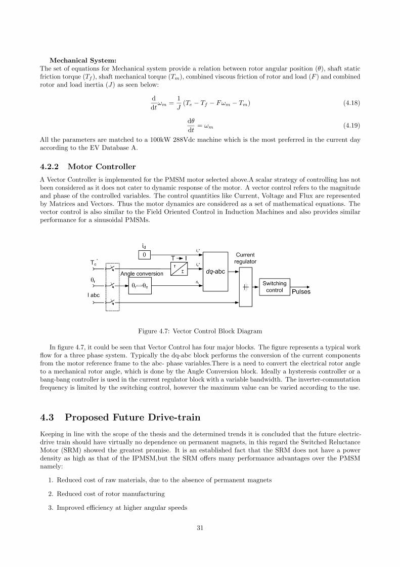
The Ld and Lq inductances signify the relation between the phase inductance and the rotor position due to thesaliency of the rotor. The inductance equation for phase a and phase b when phase c is left open (Lab) can begiven in terms of rotor angle (θe) by,

Lab = Ld + Lq + (Lq − Ld)cos

(2θe +

∏3

)(4.17)

The phase to phase variation against the rotor angle is shown as in figure 4.6

Figure 4.6: Phase vs Rotor Angle

30

Mechanical System:The set of equations for Mechanical system provide a relation between rotor angular position (θ), shaft staticfriction torque (Tf ), shaft mechanical torque (Tm), combined viscous friction of rotor and load (F ) and combinedrotor and load inertia (J) as seen below:

d

dtωm =

1

J(Te − Tf − Fωm − Tm) (4.18)

dθ

dt= ωm (4.19)

All the parameters are matched to a 100kW 288Vdc machine which is the most preferred in the current dayaccording to the EV Database A.

4.2.2 Motor Controller

A Vector Controller is implemented for the PMSM motor selected above.A scalar strategy of controlling has notbeen considered as it does not cater to dynamic response of the motor. A vector control refers to the magnitudeand phase of the controlled variables. The control quantities like Current, Voltage and Flux are representedby Matrices and Vectors. Thus the motor dynamics are considered as a set of mathematical equations. Thevector control is also similar to the Field Oriented Control in Induction Machines and also provides similarperformance for a sinusoidal PMSMs.

Figure 4.7: Vector Control Block Diagram

In figure 4.7, it could be seen that Vector Control has four major blocks. The figure represents a typical workflow for a three phase system. Typically the dq-abc block performs the conversion of the current componentsfrom the motor reference frame to the abc- phase variables.There is a need to convert the electrical rotor angleto a mechanical rotor angle, which is done by the Angle Conversion block. Ideally a hysteresis controller or abang-bang controller is used in the current regulator block with a variable bandwidth. The inverter-commutationfrequency is limited by the switching control, however the maximum value can be varied according to the use.

4.3 Proposed Future Drive-train

Keeping in line with the scope of the thesis and the determined trends it is concluded that the future electric-drive train should have virtually no dependence on permanent magnets, in this regard the Switched ReluctanceMotor (SRM) showed the greatest promise. It is an established fact that the SRM does not have a powerdensity as high as that of the IPMSM,but the SRM offers many performance advantages over the PMSMnamely:

1. Reduced cost of raw materials, due to the absence of permanent magnets

2. Reduced cost of rotor manufacturing

3. Improved efficiency at higher angular speeds

31

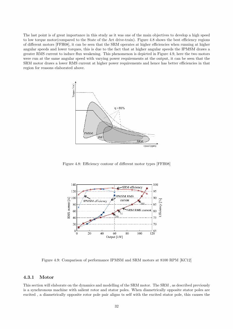
The last point is of great importance in this study as it was one of the main objectives to develop a high speedto low torque motor(compared to the State of the Art drive-train). Figure 4.8 shows the best efficiency regionsof different motors [FFH08], it can be seen that the SRM operates at higher efficiencies when running at higherangular speeds and lower torques, this is due to the fact that at higher angular speeds the IPMSM draws agreater RMS current to induce flux weakening. This phenomenon is depicted in Figure 4.9, here the two motorswere run at the same angular speed with varying power requirements at the output, it can be seen that theSRM motor draws a lower RMS current at higher power requirements and hence has better efficiencies in thatregion for reasons elaborated above.

Figure 4.8: Efficiency contour of different motor types [FFH08]

Figure 4.9: Comparison of performance IPMSM and SRM motors at 8100 RPM [KC12]

4.3.1 Motor

This section will elaborate on the dynamics and modelling of the SRM motor. The SRM , as described previouslyis a synchronous machine with salient rotor and stator poles. When diametrically opposite stator poles areexcited , a diametrically opposite rotor pole pair aligns ts self with the excited stator pole, this causes the

32

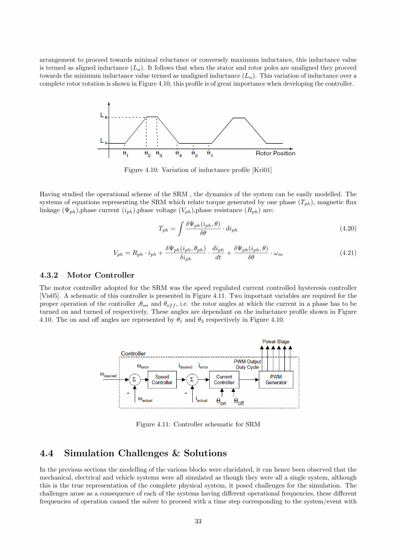
arrangement to proceed towards minimal reluctance or conversely maximum inductance, this inductance valueis termed as aligned inductance (La). It follows that when the stator and rotor poles are unaligned they proceedtowards the minimum inductance value termed as unaligned inductance (Lu). This variation of inductance over acomplete rotor rotation is shown in Figure 4.10, this profile is of great importance when developing the controller.

Figure 4.10: Variation of inductance profile [Kri01]

Having studied the operational scheme of the SRM , the dynamics of the system can be easily modelled. Thesystems of equations representing the SRM which relate torque generated by one phase (Tph), magnetic fluxlinkage (Ψph),phase current (iph),phase voltage (Vph),phase resistance (Rph) are:

Tph =

∫δΨph(iph, θ)

δθ· diph (4.20)

Vph = Rph · iph +δΨph(iph, θph)

δiph· diphdt

+δΨph(iph, θ)

δθ· ωm (4.21)

4.3.2 Motor Controller

The motor controller adopted for the SRM was the speed regulated current controlled hysteresis controller[Vis05]. A schematic of this controller is presented in Figure 4.11. Two important variables are required for theproper operation of the controller ,θon and θoff , i.e. the rotor angles at which the current in a phase has to beturned on and turned of respectively. These angles are dependant on the inductance profile shown in Figure4.10. The on and off angles are represented by θ1 and θ3 respectively in Figure 4.10.

Figure 4.11: Controller schematic for SRM

4.4 Simulation Challenges & Solutions

In the previous sections the modelling of the various blocks were elucidated, it can hence been observed that themechanical, electrical and vehicle systems were all simulated as though they were all a single system, althoughthis is the true representation of the complete physical system, it posed challenges for the simulation. Thechallenges arose as a consequence of each of the systems having different operational frequencies, these differentfrequencies of operation caused the solver to proceed with a time step corresponding to the system/event with

33

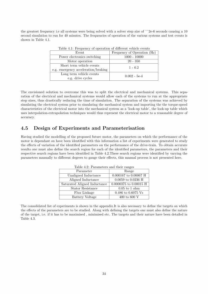
the greatest frequency i.e all systems were being solved with a solver step size of ˜˜2e-6 seconds causing a 10second simulation to run for 40 minutes. The frequencies of operation of the various systems and test events isshown in Table 4.1.

Table 4.1: Frequency of operation of different vehicle eventsEvent Frequency of Operation (Hz)

Power electronics switching 1000 - 10000Motor operation 20 - 350

Short term vehicle eventse.g. emergency acceleration/braking

1 - 0.2

Long term vehicle eventse.g. drive cycles

0.002 - 5e-4

The envisioned solution to overcome this was to split the electrical and mechanical systems. This sepa-ration of the electrical and mechanical systems would allow each of the systems to run at the appropriatestep sizes, thus drastically reducing the time of simulation. The separation of the systems was achieved bysimulating the electrical system prior to simulating the mechanical system and importing the the torque-speedcharacteristics of the electrical motor into the mechanical system as a ’look-up table’, the look-up table whichuses interpolation-extrapolation techniques would thus represent the electrical motor to a reasonable degree ofaccuracy.

4.5 Design of Experiments and Parameterisation

Having studied the modelling of the proposed future motor, the parameters on which the performance of themotor is dependant on have been identified with this information a list of experiments were generated to studythe effects of variation of the identified parameters on the performance of the drive-train. To obtain accurateresults one must also define the search region for each of the identified parameters, the parameters and theirrespective search regions have been identified in Table 4.2.These search regions were identified by varying theparameters manually to different degrees to gauge their effects, this manual process is not presented here.

Table 4.2: Parameters and their rangesParameter Range

Unaligned Inductance 0.000167 to 0.00067 HAligned Inductance 0.0059 to 0.0236 H

Saturated Aligned Inductance 0.0000375 to 0.00015 HStator Resistance 0.05 to 1 ohm

Flux Linkage 0.486 to 0.6075 VsBattery Voltage 400 to 600 V

The consolidated list of experiments is shown in the appendix.It is also necessary to define the targets on whichthe effects of the parameters are to be studied. Along with defining the targets one must also define the natureof the target, i.e. if it has to be maximised , minimised etc. The targets and their nature have been detailed inTable 4.3.

34

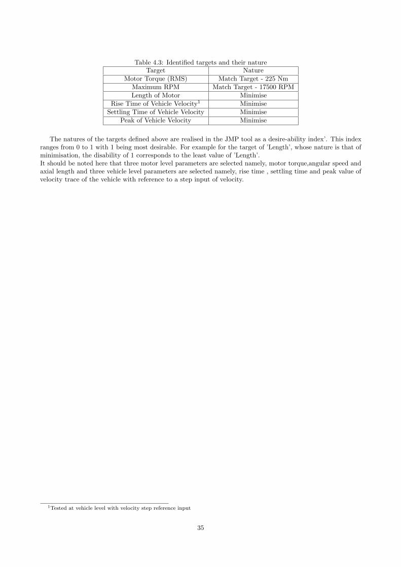
Table 4.3: Identified targets and their natureTarget Nature

Motor Torque (RMS) Match Target - 225 NmMaximum RPM Match Target - 17500 RPMLength of Motor Minimise

Rise Time of Vehicle Velocity1 MinimiseSettling Time of Vehicle Velocity Minimise

Peak of Vehicle Velocity Minimise

The natures of the targets defined above are realised in the JMP tool as a desire-ability index’. This indexranges from 0 to 1 with 1 being most desirable. For example for the target of ’Length’, whose nature is that ofminimisation, the disability of 1 corresponds to the least value of ’Length’.It should be noted here that three motor level parameters are selected namely, motor torque,angular speed andaxial length and three vehicle level parameters are selected namely, rise time , settling time and peak value ofvelocity trace of the vehicle with reference to a step input of velocity.

1Tested at vehicle level with velocity step reference input

35

36

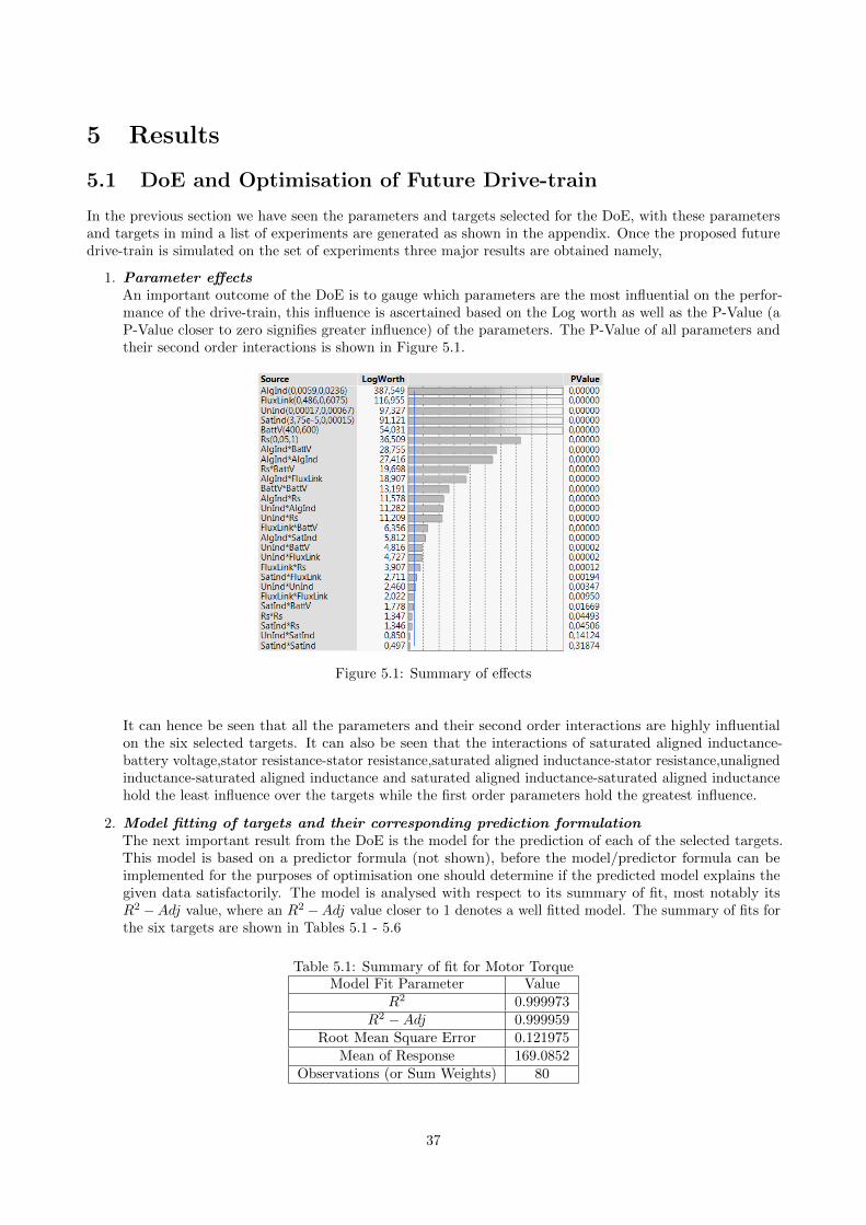
5 Results

5.1 DoE and Optimisation of Future Drive-train

In the previous section we have seen the parameters and targets selected for the DoE, with these parametersand targets in mind a list of experiments are generated as shown in the appendix. Once the proposed futuredrive-train is simulated on the set of experiments three major results are obtained namely,

1. Parameter effectsAn important outcome of the DoE is to gauge which parameters are the most influential on the perfor-mance of the drive-train, this influence is ascertained based on the Log worth as well as the P-Value (aP-Value closer to zero signifies greater influence) of the parameters. The P-Value of all parameters andtheir second order interactions is shown in Figure 5.1.

Figure 5.1: Summary of effects

It can hence be seen that all the parameters and their second order interactions are highly influentialon the six selected targets. It can also be seen that the interactions of saturated aligned inductance-battery voltage,stator resistance-stator resistance,saturated aligned inductance-stator resistance,unalignedinductance-saturated aligned inductance and saturated aligned inductance-saturated aligned inductancehold the least influence over the targets while the first order parameters hold the greatest influence.

2. Model fitting of targets and their corresponding prediction formulationThe next important result from the DoE is the model for the prediction of each of the selected targets.This model is based on a predictor formula (not shown), before the model/predictor formula can beimplemented for the purposes of optimisation one should determine if the predicted model explains thegiven data satisfactorily. The model is analysed with respect to its summary of fit, most notably itsR2 −Adj value, where an R2 −Adj value closer to 1 denotes a well fitted model. The summary of fits forthe six targets are shown in Tables 5.1 - 5.6

Table 5.1: Summary of fit for Motor TorqueModel Fit Parameter Value

R2 0.999973R2 −Adj 0.999959

Root Mean Square Error 0.121975Mean of Response 169.0852

Observations (or Sum Weights) 80

37

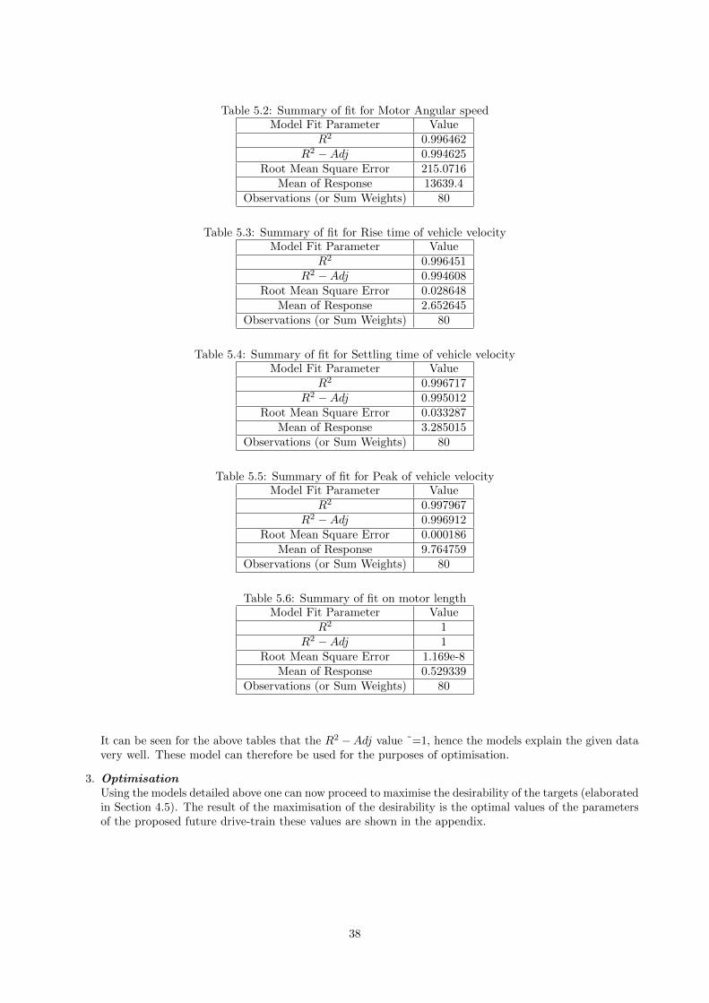
Table 5.2: Summary of fit for Motor Angular speedModel Fit Parameter Value

R2 0.996462R2 −Adj 0.994625

Root Mean Square Error 215.0716Mean of Response 13639.4

Observations (or Sum Weights) 80

Table 5.3: Summary of fit for Rise time of vehicle velocityModel Fit Parameter Value

R2 0.996451R2 −Adj 0.994608

Root Mean Square Error 0.028648Mean of Response 2.652645

Observations (or Sum Weights) 80

Table 5.4: Summary of fit for Settling time of vehicle velocityModel Fit Parameter Value

R2 0.996717R2 −Adj 0.995012

Root Mean Square Error 0.033287Mean of Response 3.285015

Observations (or Sum Weights) 80

Table 5.5: Summary of fit for Peak of vehicle velocityModel Fit Parameter Value

R2 0.997967R2 −Adj 0.996912

Root Mean Square Error 0.000186Mean of Response 9.764759

Observations (or Sum Weights) 80

Table 5.6: Summary of fit on motor lengthModel Fit Parameter Value

R2 1R2 −Adj 1

Root Mean Square Error 1.169e-8Mean of Response 0.529339

Observations (or Sum Weights) 80

It can be seen for the above tables that the R2 −Adj value ˜=1, hence the models explain the given datavery well. These model can therefore be used for the purposes of optimisation.

3. OptimisationUsing the models detailed above one can now proceed to maximise the desirability of the targets (elaboratedin Section 4.5). The result of the maximisation of the desirability is the optimal values of the parametersof the proposed future drive-train these values are shown in the appendix.

38

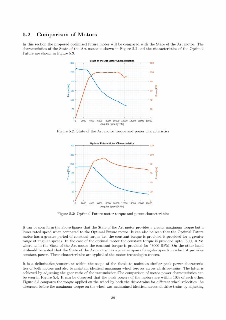
5.2 Comparison of Motors

In this section the proposed optimised future motor will be compared with the State of the Art motor. Thecharacteristics of the State of the Art motor is shown in Figure 5.2 and the characteristics of the OptimalFuture are shown in Figure 5.3.

0 2000 4000 6000 8000 10000 12000 14000 16000 18000

Angular Speed[RPM]

0

50

100

150

200

250

300

Tor

que[

Nm

]

0

20

40

60

80

100

120

Pow

er[k

W]

State of the Art Motor Characteristics

Figure 5.2: State of the Art motor torque and power characteristics

0 2000 4000 6000 8000 10000 12000 14000 16000 18000

Angular Speed[RPM]

0

50

100

150

200

250

300

Tor

que[

Nm

]

0

20

40

60

80

100

120

Pow

er[k

W]

Optimal Future Motor Characteristics

Figure 5.3: Optimal Future motor torque and power characteristics

It can be seen form the above figures that the State of the Art motor provides a greater maximum torque but alower rated speed when compared to the Optimal Future motor. It can also be seen that the Optimal Futuremotor has a greater period of constant torque i.e. the constant torque is provided is provided for a greaterrange of angular speeds. In the case of the optimal motor the constant torque is provided upto ˜5000 RPMwhere as in the State of the Art motor the constant torque is provided for ˜3000 RPM. On the other handit should be noted that the State of the Art motor has a greater span of angular speeds in which it providesconstant power. These characteristics are typical of the motor technologies chosen.

It is a delimitation/constraint within the scope of the thesis to maintain similar peak power characteris-tics of both motors and also to maintain identical maximum wheel torques across all drive-trains. The latter isachieved by adjusting the gear ratio of the transmission.The comparison of motor power characteristics canbe seen in Figure 5.4. It can be observed that the peak powers of the motors are within 10% of each other.Figure 5.5 compares the torque applied on the wheel by both the drive-trains for different wheel velocities. Asdiscussed before the maximum torque on the wheel was maintained identical across all drive-trains by adjusting

39

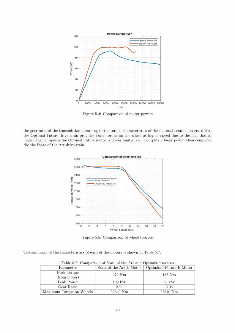
0 2000 4000 6000 8000 10000 12000 14000 16000 18000

RPM

0

20

40

60

80

100

120

Pow

er[k

W]

Power Comparison

Optimal Future DTState of the Art DT

Figure 5.4: Comparison of motor powers

the gear ratio of the transmission according to the torque characteristics of the motors.It can be observed thatthe Optimal Future drive-train provides lower torque on the wheel at higher speed due to the fact that athigher angular speeds the Optimal Future motor is power limited i.e. it outputs a lower power when comparedthe the State of the Art drive-train.

0 2 4 6 8 10 12 14 16 18 20

Wheel Speed [m/s]

1200

1400

1600

1800

2000

2200

2400

2600

2800

Tor

que

on W

heel

[Nm

]

Comparison of wheel torques

State of the Art DTOptimised Future DT

Figure 5.5: Comparison of wheel torques

The summary of the characteristics of each of the motors is shown in Table 5.7.

Table 5.7: Comparison of State of the Art and Optimised motorsParameter State of the Art E-Motor Optimised Future E-Motor

Peak Torque(from motor)

270 Nm 185 Nm

Peak Power 100 kW 93 kWGear Ratio 2.71 3.95

Maximum Torque on Wheels ˜2640 Nm ˜2640 Nm

40

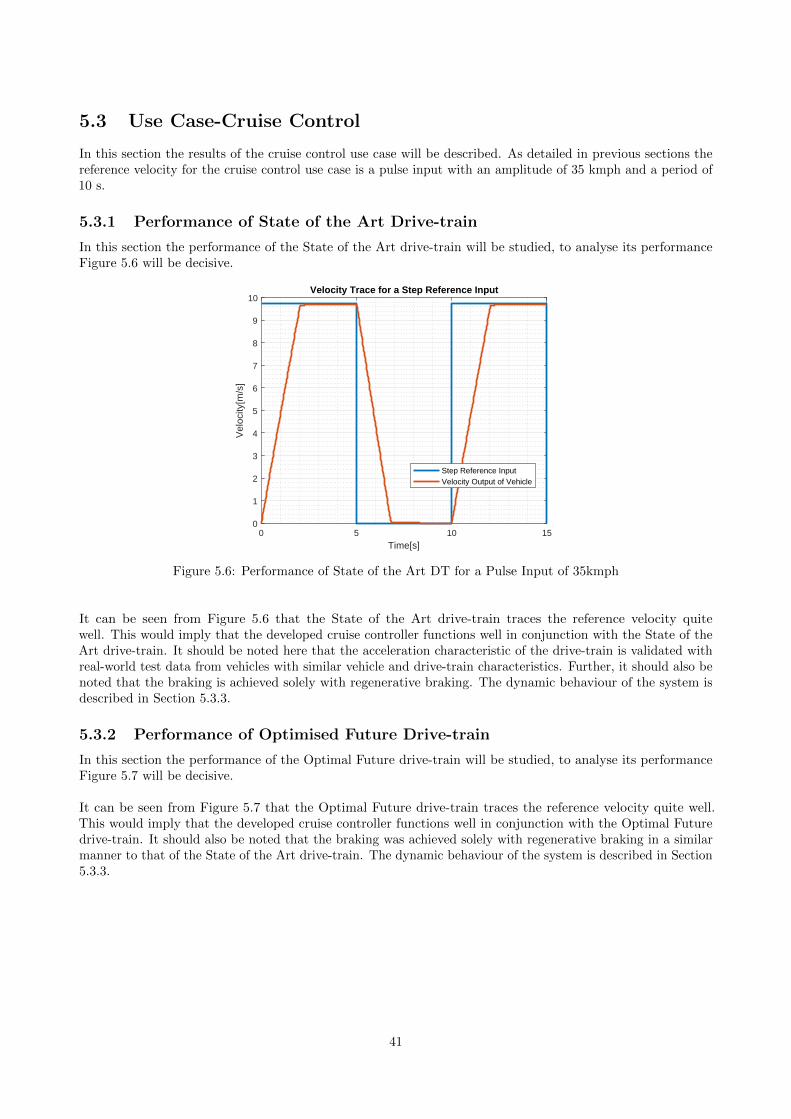
5.3 Use Case-Cruise Control

In this section the results of the cruise control use case will be described. As detailed in previous sections thereference velocity for the cruise control use case is a pulse input with an amplitude of 35 kmph and a period of10 s.

5.3.1 Performance of State of the Art Drive-train

In this section the performance of the State of the Art drive-train will be studied, to analyse its performanceFigure 5.6 will be decisive.

0 5 10 15

Time[s]

0

1

2

3

4

5

6

7

8

9

10

Vel

ocity

[m/s

]

Velocity Trace for a Step Reference Input

Step Reference InputVelocity Output of Vehicle

Figure 5.6: Performance of State of the Art DT for a Pulse Input of 35kmph

It can be seen from Figure 5.6 that the State of the Art drive-train traces the reference velocity quitewell. This would imply that the developed cruise controller functions well in conjunction with the State of theArt drive-train. It should be noted here that the acceleration characteristic of the drive-train is validated withreal-world test data from vehicles with similar vehicle and drive-train characteristics. Further, it should also benoted that the braking is achieved solely with regenerative braking. The dynamic behaviour of the system isdescribed in Section 5.3.3.

5.3.2 Performance of Optimised Future Drive-train

In this section the performance of the Optimal Future drive-train will be studied, to analyse its performanceFigure 5.7 will be decisive.

It can be seen from Figure 5.7 that the Optimal Future drive-train traces the reference velocity quite well.This would imply that the developed cruise controller functions well in conjunction with the Optimal Futuredrive-train. It should also be noted that the braking was achieved solely with regenerative braking in a similarmanner to that of the State of the Art drive-train. The dynamic behaviour of the system is described in Section5.3.3.

41

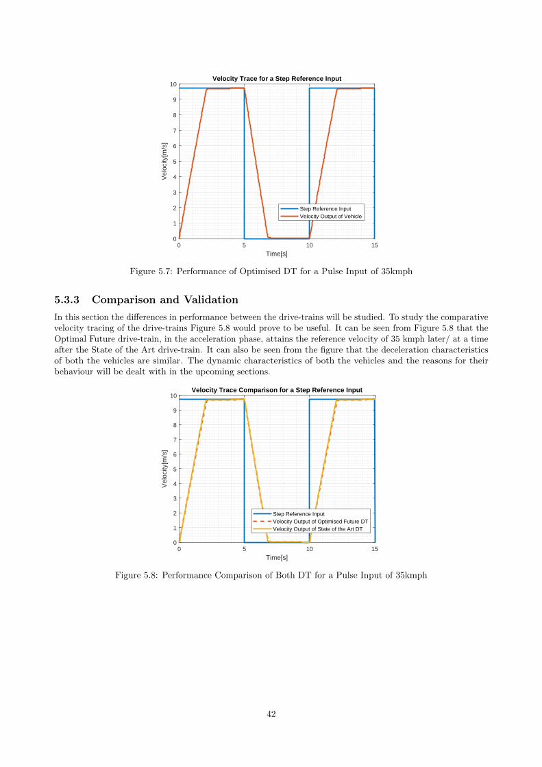
0 5 10 15

Time[s]

0

1

2

3

4

5

6

7

8

9

10

Vel

ocity

[m/s

]

Velocity Trace for a Step Reference Input

Step Reference InputVelocity Output of Vehicle

Figure 5.7: Performance of Optimised DT for a Pulse Input of 35kmph

5.3.3 Comparison and Validation

In this section the differences in performance between the drive-trains will be studied. To study the comparativevelocity tracing of the drive-trains Figure 5.8 would prove to be useful. It can be seen from Figure 5.8 that theOptimal Future drive-train, in the acceleration phase, attains the reference velocity of 35 kmph later/ at a timeafter the State of the Art drive-train. It can also be seen from the figure that the deceleration characteristicsof both the vehicles are similar. The dynamic characteristics of both the vehicles and the reasons for theirbehaviour will be dealt with in the upcoming sections.

0 5 10 15

Time[s]

0

1

2

3

4

5

6

7

8

9

10

Vel

ocity

[m/s

]

Velocity Trace Comparison for a Step Reference Input

Step Reference InputVelocity Output of Optimised Future DTVelocity Output of State of the Art DT

Figure 5.8: Performance Comparison of Both DT for a Pulse Input of 35kmph

42

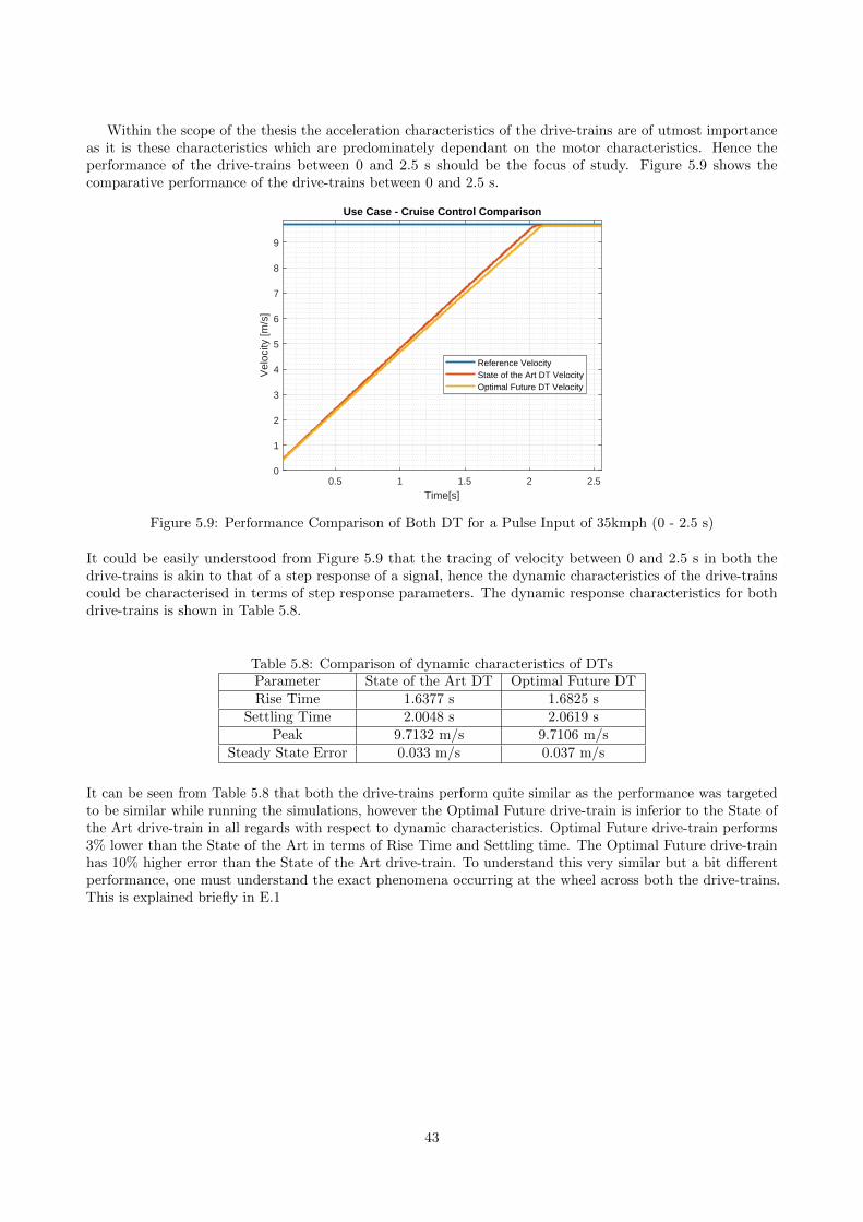
Within the scope of the thesis the acceleration characteristics of the drive-trains are of utmost importanceas it is these characteristics which are predominately dependant on the motor characteristics. Hence theperformance of the drive-trains between 0 and 2.5 s should be the focus of study. Figure 5.9 shows thecomparative performance of the drive-trains between 0 and 2.5 s.

0.5 1 1.5 2 2.5

Time[s]

0

1

2

3

4

5

6

7

8

9

Vel

ocity

[m/s

]

Use Case - Cruise Control Comparison

Reference VelocityState of the Art DT VelocityOptimal Future DT Velocity

Figure 5.9: Performance Comparison of Both DT for a Pulse Input of 35kmph (0 - 2.5 s)

It could be easily understood from Figure 5.9 that the tracing of velocity between 0 and 2.5 s in both thedrive-trains is akin to that of a step response of a signal, hence the dynamic characteristics of the drive-trainscould be characterised in terms of step response parameters. The dynamic response characteristics for bothdrive-trains is shown in Table 5.8.

Table 5.8: Comparison of dynamic characteristics of DTsParameter State of the Art DT Optimal Future DTRise Time 1.6377 s 1.6825 s

Settling Time 2.0048 s 2.0619 sPeak 9.7132 m/s 9.7106 m/s

Steady State Error 0.033 m/s 0.037 m/s

It can be seen from Table 5.8 that both the drive-trains perform quite similar as the performance was targetedto be similar while running the simulations, however the Optimal Future drive-train is inferior to the State ofthe Art drive-train in all regards with respect to dynamic characteristics. Optimal Future drive-train performs3% lower than the State of the Art in terms of Rise Time and Settling time. The Optimal Future drive-trainhas 10% higher error than the State of the Art drive-train. To understand this very similar but a bit differentperformance, one must understand the exact phenomena occurring at the wheel across both the drive-trains.This is explained briefly in E.1

43

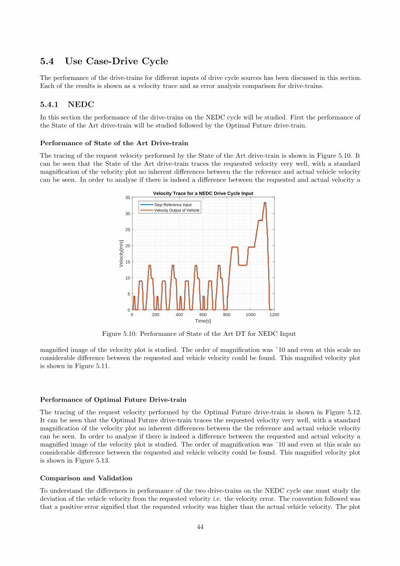
5.4 Use Case-Drive Cycle

The performance of the drive-trains for different inputs of drive cycle sources has been discussed in this section.Each of the results is shown as a velocity trace and as error analysis comparison for drive-trains.

5.4.1 NEDC

In this section the performance of the drive-trains on the NEDC cycle will be studied. First the performance ofthe State of the Art drive-train will be studied followed by the Optimal Future drive-train.

Performance of State of the Art Drive-train

The tracing of the request velocity performed by the State of the Art drive-train is shown in Figure 5.10. Itcan be seen that the State of the Art drive-train traces the requested velocity very well, with a standardmagnification of the velocity plot no inherent differences between the the reference and actual vehicle velocitycan be seen. In order to analyse if there is indeed a difference between the requested and actual velocity a

0 200 400 600 800 1000 1200

Time[s]

0

5

10

15

20

25

30

35

Vel

ocity

[m/s

]

Velocity Trace for a NEDC Drive Cycle Input

Step Reference InputVelocity Output of Vehicle

Figure 5.10: Performance of State of the Art DT for NEDC Input

magnified image of the velocity plot is studied. The order of magnification was ˜10 and even at this scale noconsiderable difference between the requested and vehicle velocity could be found. This magnified velocity plotis shown in Figure 5.11.

Performance of Optimal Future Drive-train

The tracing of the request velocity performed by the Optimal Future drive-train is shown in Figure 5.12.It can be seen that the Optimal Future drive-train traces the requested velocity very well, with a standardmagnification of the velocity plot no inherent differences between the the reference and actual vehicle velocitycan be seen. In order to analyse if there is indeed a difference between the requested and actual velocity amagnified image of the velocity plot is studied. The order of magnification was ˜10 and even at this scale noconsiderable difference between the requested and vehicle velocity could be found. This magnified velocity plotis shown in Figure 5.13.

Comparison and Validation

To understand the differences in performance of the two drive-trains on the NEDC cycle one must study thedeviation of the vehicle velocity from the requested velocity i.e. the velocity error. The convention followed wasthat a positive error signified that the requested velocity was higher than the actual vehicle velocity. The plot

44

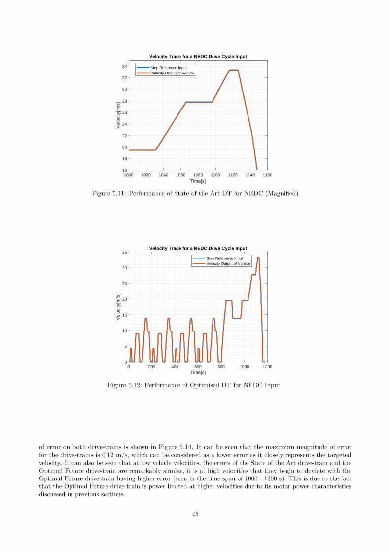
1000 1020 1040 1060 1080 1100 1120 1140 1160

Time[s]

16

18

20

22

24

26

28

30

32

34

Vel

ocity

[m/s

]

Velocity Trace for a NEDC Drive Cycle Input

Step Reference InputVelocity Output of Vehicle

Figure 5.11: Performance of State of the Art DT for NEDC (Magnified)

0 200 400 600 800 1000 1200

Time[s]

0

5

10

15

20

25

30

35

Vel

ocity

[m/s

]

Velocity Trace for a NEDC Drive Cycle Input

Step Reference InputVelocity Output of Vehicle

Figure 5.12: Performance of Optimised DT for NEDC Input

of error on both drive-trains is shown in Figure 5.14. It can be seen that the maximum magnitude of errorfor the drive-trains is 0.12 m/s, which can be considered as a lower error as it closely represents the targetedvelocity. It can also be seen that at low vehicle velocities, the errors of the State of the Art drive-train and theOptimal Future drive-train are remarkably similar, it is at high velocities that they begin to deviate with theOptimal Future drive-train having higher error (seen in the time span of 1000 - 1200 s). This is due to the factthat the Optimal Future drive-train is power limited at higher velocities due to its motor power characteristicsdiscussed in previous sections.

45

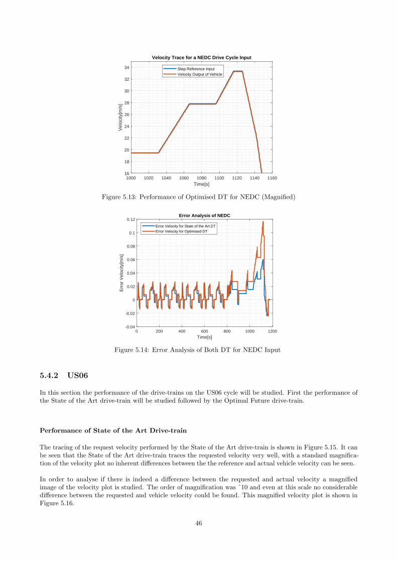
1000 1020 1040 1060 1080 1100 1120 1140 1160

Time[s]

16

18

20

22

24

26

28

30

32

34

Vel

ocity

[m/s

]

Velocity Trace for a NEDC Drive Cycle Input

Step Reference InputVelocity Output of Vehicle

Figure 5.13: Performance of Optimised DT for NEDC (Magnified)

0 200 400 600 800 1000 1200

Time[s]

-0.04

-0.02

0

0.02

0.04

0.06

0.08

0.1

0.12

Err

or V

eloc

ity[m

/s]

Error Analysis of NEDC

Error Velocity for State of the Art DTError Velocity for Optimised DT

Figure 5.14: Error Analysis of Both DT for NEDC Input

5.4.2 US06

In this section the performance of the drive-trains on the US06 cycle will be studied. First the performance ofthe State of the Art drive-train will be studied followed by the Optimal Future drive-train.

Performance of State of the Art Drive-train

The tracing of the request velocity performed by the State of the Art drive-train is shown in Figure 5.15. It canbe seen that the State of the Art drive-train traces the requested velocity very well, with a standard magnifica-tion of the velocity plot no inherent differences between the the reference and actual vehicle velocity can be seen.

In order to analyse if there is indeed a difference between the requested and actual velocity a magnifiedimage of the velocity plot is studied. The order of magnification was ˜10 and even at this scale no considerabledifference between the requested and vehicle velocity could be found. This magnified velocity plot is shown inFigure 5.16.

46

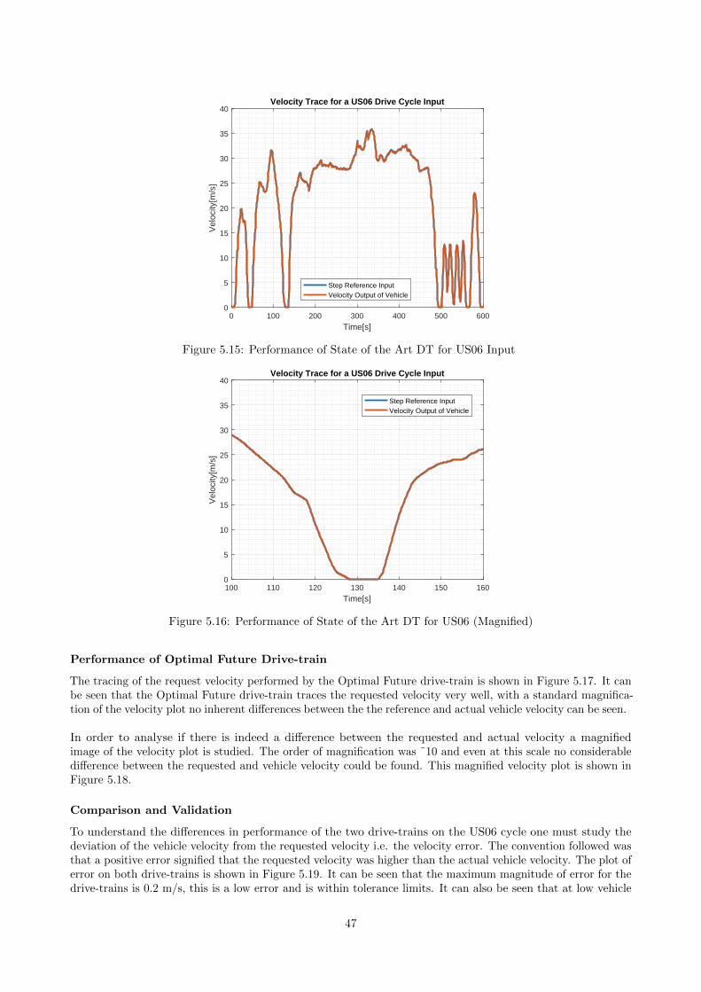
0 100 200 300 400 500 600

Time[s]

0

5

10

15

20

25

30

35

40

Vel

ocity

[m/s

]

Velocity Trace for a US06 Drive Cycle Input

Step Reference InputVelocity Output of Vehicle

Figure 5.15: Performance of State of the Art DT for US06 Input

100 110 120 130 140 150 160

Time[s]

0

5

10

15

20

25

30

35

40

Vel

ocity

[m/s

]

Velocity Trace for a US06 Drive Cycle Input

Step Reference InputVelocity Output of Vehicle

Figure 5.16: Performance of State of the Art DT for US06 (Magnified)

Performance of Optimal Future Drive-train

The tracing of the request velocity performed by the Optimal Future drive-train is shown in Figure 5.17. It canbe seen that the Optimal Future drive-train traces the requested velocity very well, with a standard magnifica-tion of the velocity plot no inherent differences between the the reference and actual vehicle velocity can be seen.

In order to analyse if there is indeed a difference between the requested and actual velocity a magnifiedimage of the velocity plot is studied. The order of magnification was ˜10 and even at this scale no considerabledifference between the requested and vehicle velocity could be found. This magnified velocity plot is shown inFigure 5.18.

Comparison and Validation

To understand the differences in performance of the two drive-trains on the US06 cycle one must study thedeviation of the vehicle velocity from the requested velocity i.e. the velocity error. The convention followed wasthat a positive error signified that the requested velocity was higher than the actual vehicle velocity. The plot oferror on both drive-trains is shown in Figure 5.19. It can be seen that the maximum magnitude of error for thedrive-trains is 0.2 m/s, this is a low error and is within tolerance limits. It can also be seen that at low vehicle

47

0 100 200 300 400 500 600

Time[s]

0

5

10

15

20

25

30

35

40

Vel

ocity

[m/s

]

Velocity Trace for a US06 Drive Cycle Input

Step Reference InputVelocity Output of Vehicle

Figure 5.17: Performance of Optimised DT for US06 Input

100 110 120 130 140 150 160

Time[s]

0

5

10

15

20

25

30

35

40

Vel

ocity

[m/s

]

Velocity Trace for a US06 Drive Cycle Input

Step Reference InputVelocity Output of Vehicle

Figure 5.18: Performance of Optimised DT for US06 Input (Magnified)

velocities, the errors of the State of the Art drive-train and the Optimal Future drive-train are remarkablysimilar, it is at high velocities that they begin to deviate with the Optimal Future drive-train having highererror, this is represented by peaks in the error plot of the Optimal Future drive-train, these peaks can be seenin the regions around 100 s, 330 s and 580 s, it is at these times that there is a high velocity/accelerationdemand. This error trend is due to the fact that the Optimal Future drive-train is power limited at highervelocities due to its motor power characteristics discussed in previous sections.

5.4.3 WLTP Class 3

In this section the performance of the drive-trains on the WLTP Class 3 cycle will be studied. First theperformance of the State of the Art drive-train will be studied followed by the Optimal Future drive-train.

Performance of State of the Art Drive-train

The tracing of the request velocity performed by the State of the Art drive-train is shown in Figure 5.20. It canbe seen that the State of the Art drive-train traces the requested velocity very well, with a standard magnifica-tion of the velocity plot no inherent differences between the the reference and actual vehicle velocity can be seen.

48

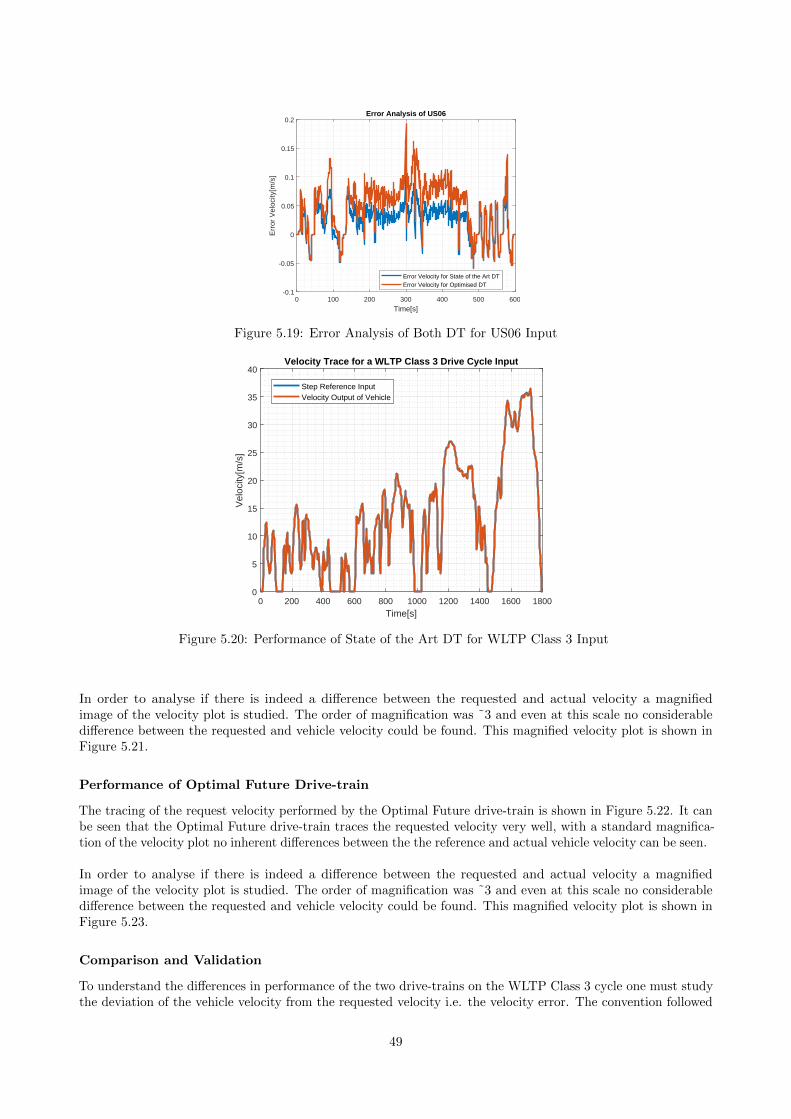
0 100 200 300 400 500 600

Time[s]

-0.1

-0.05

0

0.05

0.1

0.15

0.2

Err

or V

eloc

ity[m

/s]

Error Analysis of US06

Error Velocity for State of the Art DTError Velocity for Optimised DT

Figure 5.19: Error Analysis of Both DT for US06 Input

0 200 400 600 800 1000 1200 1400 1600 1800

Time[s]

0

5

10

15

20

25

30

35

40

Vel

ocity

[m/s

]

Velocity Trace for a WLTP Class 3 Drive Cycle Input

Step Reference InputVelocity Output of Vehicle

Figure 5.20: Performance of State of the Art DT for WLTP Class 3 Input

In order to analyse if there is indeed a difference between the requested and actual velocity a magnifiedimage of the velocity plot is studied. The order of magnification was ˜3 and even at this scale no considerabledifference between the requested and vehicle velocity could be found. This magnified velocity plot is shown inFigure 5.21.

Performance of Optimal Future Drive-train

The tracing of the request velocity performed by the Optimal Future drive-train is shown in Figure 5.22. It canbe seen that the Optimal Future drive-train traces the requested velocity very well, with a standard magnifica-tion of the velocity plot no inherent differences between the the reference and actual vehicle velocity can be seen.

In order to analyse if there is indeed a difference between the requested and actual velocity a magnifiedimage of the velocity plot is studied. The order of magnification was ˜3 and even at this scale no considerabledifference between the requested and vehicle velocity could be found. This magnified velocity plot is shown inFigure 5.23.

Comparison and Validation

To understand the differences in performance of the two drive-trains on the WLTP Class 3 cycle one must studythe deviation of the vehicle velocity from the requested velocity i.e. the velocity error. The convention followed

49

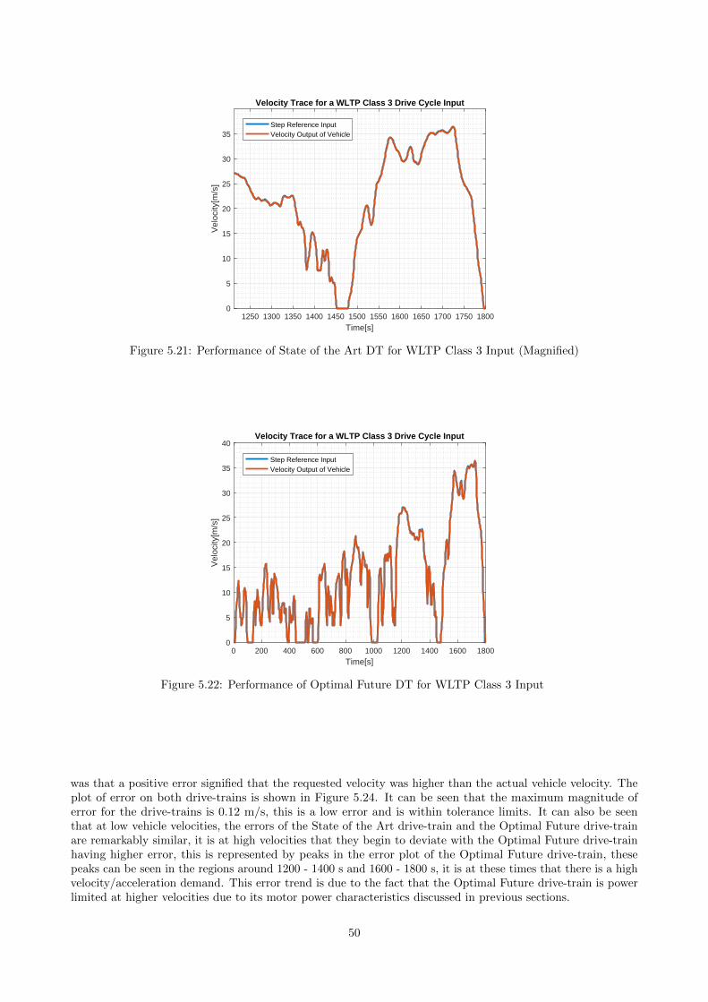
1250 1300 1350 1400 1450 1500 1550 1600 1650 1700 1750 1800

Time[s]

0

5

10

15

20

25

30

35

Vel

ocity

[m/s

]

Velocity Trace for a WLTP Class 3 Drive Cycle Input

Step Reference InputVelocity Output of Vehicle

Figure 5.21: Performance of State of the Art DT for WLTP Class 3 Input (Magnified)

0 200 400 600 800 1000 1200 1400 1600 1800

Time[s]

0

5

10

15

20

25

30

35

40

Vel

ocity

[m/s

]

Velocity Trace for a WLTP Class 3 Drive Cycle Input

Step Reference InputVelocity Output of Vehicle

Figure 5.22: Performance of Optimal Future DT for WLTP Class 3 Input

was that a positive error signified that the requested velocity was higher than the actual vehicle velocity. Theplot of error on both drive-trains is shown in Figure 5.24. It can be seen that the maximum magnitude oferror for the drive-trains is 0.12 m/s, this is a low error and is within tolerance limits. It can also be seenthat at low vehicle velocities, the errors of the State of the Art drive-train and the Optimal Future drive-trainare remarkably similar, it is at high velocities that they begin to deviate with the Optimal Future drive-trainhaving higher error, this is represented by peaks in the error plot of the Optimal Future drive-train, thesepeaks can be seen in the regions around 1200 - 1400 s and 1600 - 1800 s, it is at these times that there is a highvelocity/acceleration demand. This error trend is due to the fact that the Optimal Future drive-train is powerlimited at higher velocities due to its motor power characteristics discussed in previous sections.

50

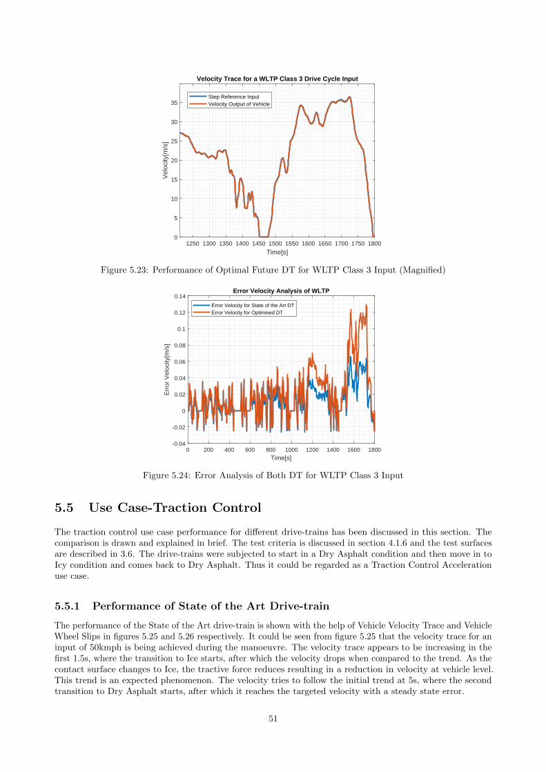
1250 1300 1350 1400 1450 1500 1550 1600 1650 1700 1750 1800

Time[s]

0

5

10

15

20

25

30

35

Vel

ocity

[m/s

]

Velocity Trace for a WLTP Class 3 Drive Cycle Input

Step Reference InputVelocity Output of Vehicle

Figure 5.23: Performance of Optimal Future DT for WLTP Class 3 Input (Magnified)

0 200 400 600 800 1000 1200 1400 1600 1800

Time[s]

-0.04

-0.02

0

0.02

0.04

0.06

0.08

0.1

0.12

0.14

Err

or V

eloc

ity[m

/s]

Error Velocity Analysis of WLTP

Error Velocity for State of the Art DTError Velocity for Optimised DT

Figure 5.24: Error Analysis of Both DT for WLTP Class 3 Input

5.5 Use Case-Traction Control

The traction control use case performance for different drive-trains has been discussed in this section. Thecomparison is drawn and explained in brief. The test criteria is discussed in section 4.1.6 and the test surfacesare described in 3.6. The drive-trains were subjected to start in a Dry Asphalt condition and then move in toIcy condition and comes back to Dry Asphalt. Thus it could be regarded as a Traction Control Accelerationuse case.

5.5.1 Performance of State of the Art Drive-train

The performance of the State of the Art drive-train is shown with the help of Vehicle Velocity Trace and VehicleWheel Slips in figures 5.25 and 5.26 respectively. It could be seen from figure 5.25 that the velocity trace for aninput of 50kmph is being achieved during the manoeuvre. The velocity trace appears to be increasing in thefirst 1.5s, where the transition to Ice starts, after which the velocity drops when compared to the trend. As thecontact surface changes to Ice, the tractive force reduces resulting in a reduction in velocity at vehicle level.This trend is an expected phenomenon. The velocity tries to follow the initial trend at 5s, where the secondtransition to Dry Asphalt starts, after which it reaches the targeted velocity with a steady state error.

51

0 1 2 3 4 5 6 7 8 9 10

Time[s]

0

5

10

15

Vel

ocity

[m/s

]

Velocity Trace for a TCS Inputs

Step Reference InputVelocity Output of Vehicle

Figure 5.25: Velocity Trace of State of the Art DT for TCS Inputs

The targeted wheel slip for the manoeuvre is 0.15 or a 15% slip, as also can be seen from figure 5.26. Whenthe vehicle is in the Dry Asphalt region, the slip tends to increase to 0.15 and is maintained by the controllerat 0.15 till it reaches 1.5. As it moves into the Ice surface the wheel slip shoots up beyond 0.2, which is anexpected trend, after which the controller tries to even out the slip back to 0.15. At 5s, as the vehicle entersthe Dry Asphalt region the wheel slip dips down towards zero slip, indicating a reduction in tractive force.The controller pitches in to maintain the slip at 0.15 until the vehicle reaches the requested velocity. As thevehicle reaches the requested velocity, the wheel slip fluctuates around zero slip due to the steady state error invelocity of the vehicle when compared to the requested velocity.

0 1 2 3 4 5 6 7 8 9 10

Time[s]

-0.05

0

0.05

0.1

0.15

0.2

0.25

Slip

[rat

io]

Wheel Slip for a TCS Input

Figure 5.26: Wheel Slip Trace of State of the Art DT for TCS Inputs

5.5.2 Performance of Optimised Future Drive-train

The performance of the Optimised Future drive-train is shown with the help of Vehicle Velocity Trace andVehicle Wheel Slips in figures 5.27 and 5.28 respectively. The velocity trend follows the same trend as discussedin section 5.5. However the velocities reached with respect to time is different compared to State of the Artdrive-train. This will however be discussed in the next section. The targeted wheel slip for the manoeuvre is0.15 or a 15% slip, as also can be seen from figure 5.28. The Wheel Slip trend matches to the trend depictedfor the State of the Art drive-train, however the slip ratios being traced are a bit different from the State of theArt drive-train and this would be discussed in the next section.

52

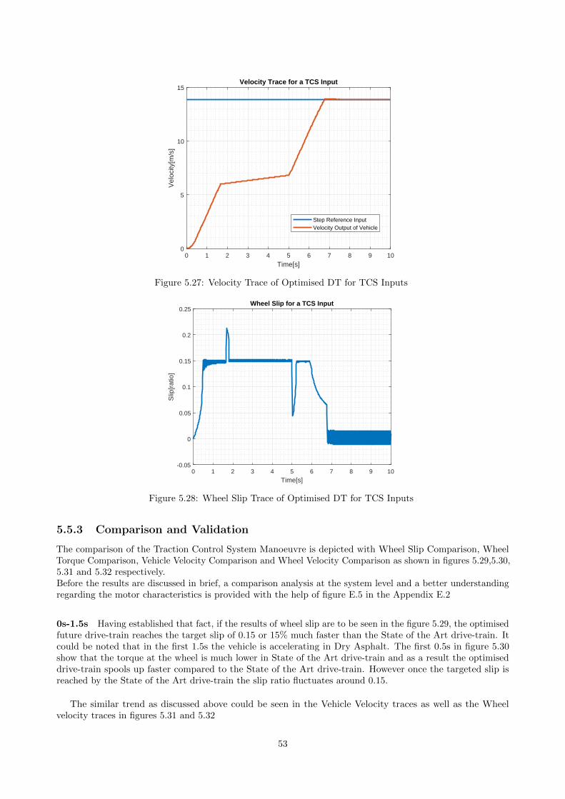
0 1 2 3 4 5 6 7 8 9 10

Time[s]

0

5

10

15

Vel

ocity

[m/s

]

Velocity Trace for a TCS Input

Step Reference InputVelocity Output of Vehicle

Figure 5.27: Velocity Trace of Optimised DT for TCS Inputs

0 1 2 3 4 5 6 7 8 9 10

Time[s]

-0.05

0

0.05

0.1

0.15

0.2

0.25

Slip

[rat

io]

Wheel Slip for a TCS Input

Figure 5.28: Wheel Slip Trace of Optimised DT for TCS Inputs

5.5.3 Comparison and Validation

The comparison of the Traction Control System Manoeuvre is depicted with Wheel Slip Comparison, WheelTorque Comparison, Vehicle Velocity Comparison and Wheel Velocity Comparison as shown in figures 5.29,5.30,5.31 and 5.32 respectively.Before the results are discussed in brief, a comparison analysis at the system level and a better understandingregarding the motor characteristics is provided with the help of figure E.5 in the Appendix E.2

0s-1.5s Having established that fact, if the results of wheel slip are to be seen in the figure 5.29, the optimisedfuture drive-train reaches the target slip of 0.15 or 15% much faster than the State of the Art drive-train. Itcould be noted that in the first 1.5s the vehicle is accelerating in Dry Asphalt. The first 0.5s in figure 5.30show that the torque at the wheel is much lower in State of the Art drive-train and as a result the optimiseddrive-train spools up faster compared to the State of the Art drive-train. However once the targeted slip isreached by the State of the Art drive-train the slip ratio fluctuates around 0.15.

The similar trend as discussed above could be seen in the Vehicle Velocity traces as well as the Wheelvelocity traces in figures 5.31 and 5.32

53

0 1 2 3 4 5 6 7 8 9 10

Time [s]

-0.05

0

0.05

0.1

0.15

0.2

0.25

Slip

ratio

Slip Ratio Comparison

State of the Art DTOptimal Future DT

Figure 5.29: Slip Comparison for Both DT for TCSInputs

0 1 2 3 4 5 6 7 8 9 10

Time, s

-400

-200

0

200

400

600

800

1000

1200

t, N

*m

Torque on Wheel Profile

State of the Art DTOptimal Future DT

Figure 5.30: Torque on Wheel Comparison for Both DTfor TCS Inputs

0 1 2 3 4 5 6 7 8 9 10

Time [s]

0

5

10

15

Velo

city

[m/s

]

Use Case - Traction Control Velocity Trace

State of the Art DTOptimal Future DTReference

Figure 5.31: Vehicle Velocity Comparison for Both DTfor TCS Inputs

0 1 2 3 4 5 6 7 8 9 10

Time, s

0

5

10

15

20

25

30

35

40

45

50

w, ra

d/s

Angular Speed of Wheels

State of the Art DTOptimal Future DT

Figure 5.32: Wheel Velocity Comparison for Both DTfor TCS Inputs

1.5s-5s As the vehicle enters the Ice Patch from the Dry Asphalt region, a sudden spike could be seen in theslip comparison figure 5.29 in both the drive-trains. This certainly suggests the loss of tractive force, however itcould be seen that the optimised future drive-train has a better accuracy and traces back to slip of 0.15 muchfaster than the State of the Art drive-train. This could be attributed to the motor characteristics. The torqueon the wheel drops down to slightly lower values than that of State of the Art drive-train.

5s-10s In this phase the vehicle is entering back into the Dry Asphalt region from Ice. From the Velocityfigure 5.31 it could be seen that both the drive-trains have similar trend till 5.8S. However both the velocitylines converge as they near the requested velocity. It could be seen from the figure 5.32 that there is a crossoverin the angular velocities of the wheel. The main reason for this could be seen in the figure 5.30, where theTorque drops off at 5.8s for the Optimised Future drive-train when compared to the State of the Art drive-train.This is typically the motor characteristic, as the Optimised Future Motor lacks the ability to provide the

54

torque required at higher speeds as compared to the State of the Art drive-train. It could however be seen asa trade-off between a faster response in an Icy patch and faster drop-off of torque at a higher speeds as thetargeted velocity is approached.

55

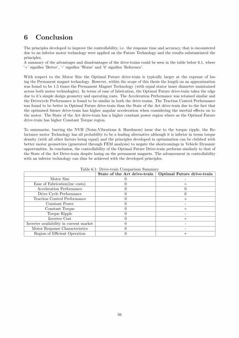
6 Conclusion

The principles developed to improve the controllability, i.e. the response time and accuracy, that is encountereddue to an inferior motor technology were applied on the Future Technology and the results substantiated theprinciples.A summary of the advantages and disadvantages of the drive-trains could be seen in the table below 6.1, where’+’ signifies ’Better’, ’-’ signifies ’Worse’ and ’0’ signifies ’Reference’.

With respect to the Motor Size the Optimal Future drive-train is typically larger at the expense of los-ing the Permanent magnet technology. However, within the scope of this thesis the length on an approximationwas found to be 1.5 times the Permanent Magnet Technology (with equal stator inner diameter maintainedacross both motor technologies). In terms of ease of fabrication, the Optimal Future drive-train takes the edgedue to it’s simple design geometry and operating costs. The Acceleration Performance was retained similar andthe Drivecycle Performance is found to be similar in both the drive-trains. The Traction Control Performancewas found to be better in Optimal Future drive-train than the State of the Art drive-train due to the fact thatthe optimised future drive-train has higher angular acceleration when considering the inertial effects on tothe motor. The State of the Art drive-train has a higher constant power region where as the Optimal Futuredrive-train has higher Constant Torque region.

To summarise, barring the NVH (Noise,Vibrations & Harshness) issue due to the torque ripple, the Re-luctance motor Technology has all probability to be a leading alternative although it is inferior in terms torquedensity (with all other factors being equal) and the principles developed in optimisation can be clubbed withbetter motor geometries (generated through FEM analysis) to negate the shortcomings in Vehicle Dynamicopportunities. In conclusion, the controllability of the Optimal Future Drive-train performs similarly to that ofthe State of the Art Drive-train despite losing on the permanent magnets. The advancement in controllabilitywith an inferior technology can thus be achieved with the developed principles.

Table 6.1: Drive-train Comparison SummaryState of the Art drive-train Optimal Future drive-train

Motor Size 0 -Ease of Fabrication(inc costs) 0 +

Acceleration Performance 0 0Drive Cycle Performance 0 0

Traction Control Performance 0 +Constant Power 0 -Constant Torque 0 +

Torque Ripple 0 -Inverter Cost 0 +

Inverter availability in current market 0 -Motor Response Characteristics 0 -Region of Efficient Operation 0 +

56

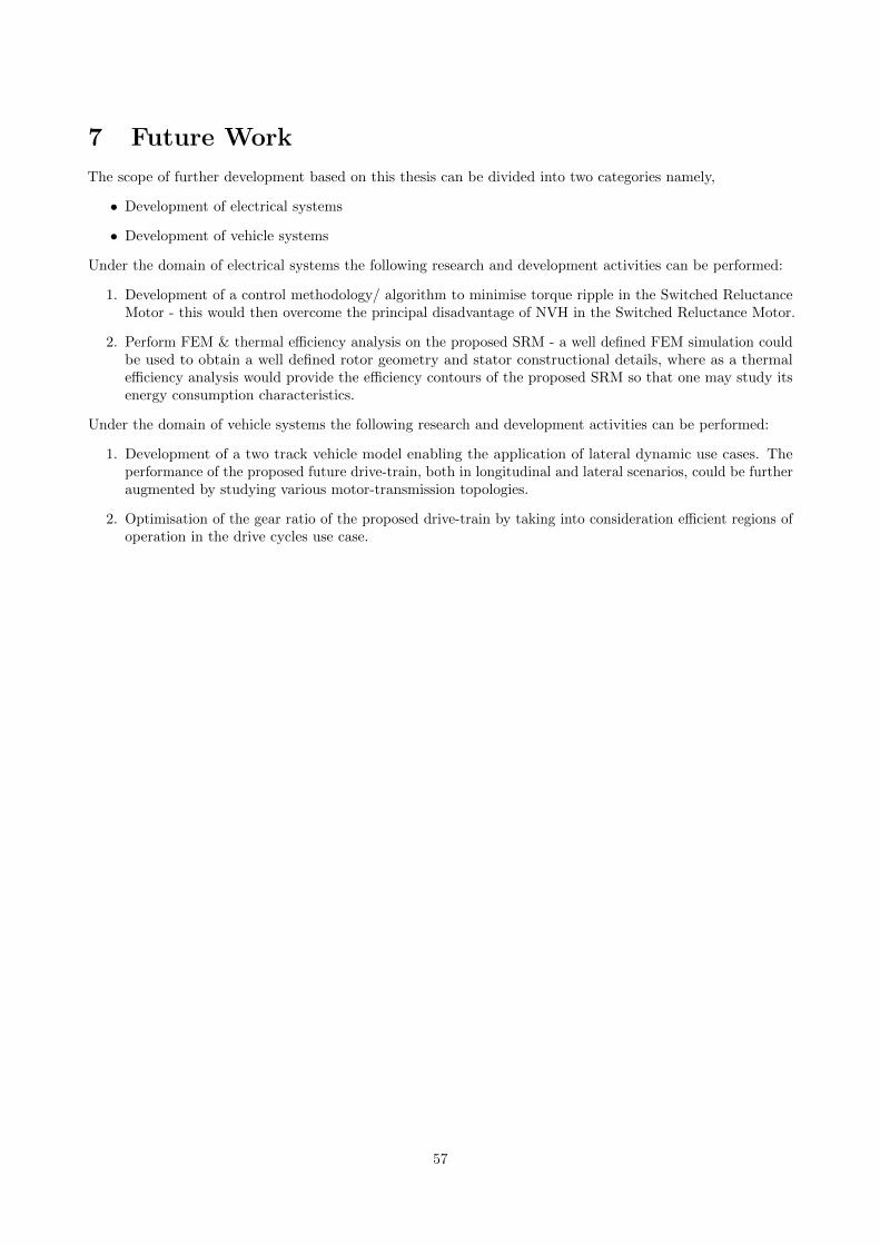
7 Future Work

The scope of further development based on this thesis can be divided into two categories namely,

• Development of electrical systems

• Development of vehicle systems

Under the domain of electrical systems the following research and development activities can be performed:

1. Development of a control methodology/ algorithm to minimise torque ripple in the Switched ReluctanceMotor - this would then overcome the principal disadvantage of NVH in the Switched Reluctance Motor.

2. Perform FEM & thermal efficiency analysis on the proposed SRM - a well defined FEM simulation couldbe used to obtain a well defined rotor geometry and stator constructional details, where as a thermalefficiency analysis would provide the efficiency contours of the proposed SRM so that one may study itsenergy consumption characteristics.

Under the domain of vehicle systems the following research and development activities can be performed:

1. Development of a two track vehicle model enabling the application of lateral dynamic use cases. Theperformance of the proposed future drive-train, both in longitudinal and lateral scenarios, could be furtheraugmented by studying various motor-transmission topologies.

2. Optimisation of the gear ratio of the proposed drive-train by taking into consideration efficient regions ofoperation in the drive cycles use case.

57

References

[12] NIST/SEMATECH e-Handbook of Statistical Methods. Market Research. NIST/SEMATECH, 2012.url: http://www.itl.nist.gov/div898/handbook/.

[17a] DESIGN OF EXPERIMENTS (DOE) TUTORIAL. Tutorial. ASQ, 2017. url: http://asq.org / learn - about - quality / data - collection - analysis - tools / overview / design - of -

experiments-tutorial.html.[17b] Linear Induction Motor. Market Research. Circuit Globe, 2017. url: https://circuitglobe.

com/linear-induction-motor.html.[17c] Permanent Magnet Synchronous Motor (PMSM) Market is Expected to Garner $31.1 Billion, Glob-

ally, by 2022. Market Research. Allied Market Research, 2017. url: https://alliedmarketresearch.wordpress.com/2017/02/03/permanent- magnet- synchronous- motor- pmsm- market- is-

expected-to-garner-31-1-billion-globally-by-2022/.[17d] Switched Reluctance Motor (SRM). Market Research. EMWorks, 2017. url: https://www.emworks.

com/blog/motor-design/switched-reluctance-motor-electric-vehicles.[ARI15] A. ARIKERE. Vehicle Dynamic Opportunities in Electrified Vehicles for Active Safety Interventions

(2015).[Bar+09] T. J. Barlow et al. A Reference Book of Driving Cycles for Use in the Measurement of Road Vehicle

Emissions (2009).[CG17] P. Cazzola and M. Gorner. Global EV Outlook 2017 (2017).[CS17] A. Cooper and K. Schefter. Plug-in Electric Vehicle Forecast: 2016-2025. IEI Report (2017).[Err+17] M. Erriquez et al. Trends in Electric Vehicle Design (2017).[FFH08] T. Finken, M. Felden, and K. Hameyer. Comparison and design of different electrical machine

types regarding their applicability in hybrid electrical vehicles. 18th International Conference onElectrical Machines, 2008. ICEM 2008. (2008).

[IE17] A. C. (IEI) and K. S. (EEI). Plug-in Electric Vehicle Forecast: 2016-2025. Institute for ElectricInnovation, 2017.

[INC] G. V. R. INC. Permanent Magnet Market Size, Share Trend Analysis Report By Product(Ferrite Magnet, Rare Earth), By Application (Automotive, Electronics, Industrial) By Region,And Segment Forecasts, 2018 - 2024. Global Permanent Magnet Market Share, Industry Report,2018-2024 ().

[KC12] K. Kiyota and A. Chiba. Design of Switched Reluctance Motor Competitive to 60-kW IPMSM inThird-Generation Hybrid Electric Vehicle. IEEE TRANSACTIONS ON INDUSTRY APPLICA-TIONS (2012).

[KF16] B. Kerdsup and N. H. Fuengwarodsakul. Performance and cost comparison of reluctance motorsused for electric bicycles (2016).

[Kri01] R. Krishnan. SWITCHED RELUCTANCE MOTOR DRIVES (2001).[Pal+18] K. Palmera et al. Total cost of ownership and market share for hybrid and electric vehicles in the

UK, US and Japan. Applied Energy 209 (2018), 108–119.[Raj13] K. Rajashekara. Present Status and Future Trends in Electric Vehicle Propulsion Technologies

(2013).[UC07] S. Unnasch and M. Chan. Full fuel cycle assessment Tank to wheels emissions And energy

consumption (2007).[UnN+17] F. Un-Noor et al. A Comprehensive Study of Key Electric Vehicle (EV) Components, Technologies,

Challenges, Impacts, and Future Direction of Development (2017).[Vis05] R. Visinka. 3-Phase Switched Reluctance (SR) Sensorless Motor Control Using a 56F80x, 56F8100

or 56F8300 Device (2005).[Zet07] C. Zetterqvist. Powertrain modelling and control algorithms for traction control. Department of

Electrical Engineering,Linkopings Universitet, 2007.

58

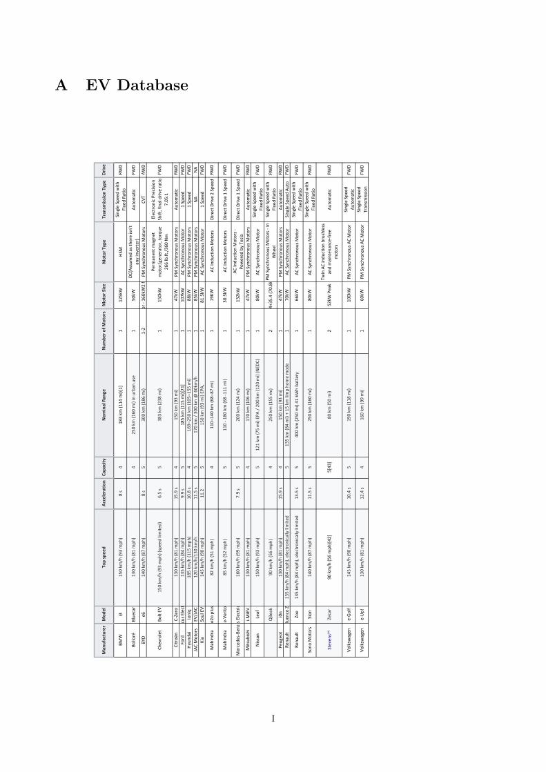
A EV Database

BMW

i315

0 km

/h (9

3 mph

)8 s

418

3 km

 (114

 mi)[1]

112

5kW

HSM

Sing

le Spe

ed with

 Fixed Ra

tioRW

D

Bollo

réBlue

car

130 km

/h (8

1 mph

)4

250 km

 (160

 mi) in urban

 use

150

kWDC(As

sumed

 as the

re isn't 

any inverter)

Automatic

FWD

BYD

e614

0 km

/h (8

7 mph

)8 s

530

0 km

 (186

 mi)

1-2

1 Sing

le M

otor - 16

0kW2 Motors-75

+40

PM Syn

chrono

us M

otors

CVT

AWD

Chevrolet

Bolt EV

150 km

/h (9

3 mph

) (spee

d lim

ited)

6.5 s

538

3 km

 (238

 mi)

115

0kW

Perm

anen

t magne

t motor/gen

erator, torqu

e 26

6 lb.ft./36

0 Nm

Electron

ic Precision

 Sh

ift, final driv

e ratio

 7.05

:1FW

D

Citroë

nC-Ze

ro13

0 km

/h (8

1 mph

)15

.9 s

415

0 km

 (93 mi)

147

kWPM

 Syn

chrono

us M

otors

Automatic

RWD

Ford

Focu

s Electric

135 km

/h (8

4 mph

)9.9 s

518

5 km

 (115

 mi)[21

]1

107k

WAC

 Syn

chrono

us M

otor

1 Sp

eed

FWD

Hyu

ndai

Ioniq

185 km

/h (1

15 m

ph)

10.8 s

416

9–25

0 km

 (105

–155

 mi)

188

kWPM

 Syn

chrono

us M

otors

1 Sp

eed

FWD

JAC Motors

JAC J3 EV/JAC IEV 6S

120 km

/h/130

 km/h

11.5 s

517

0 km

 / 30

0 km

 @ 60k

m/h

185

kWPM

 Syn

chrono

us M

otors

NA

NA

Kia

Soul EV

145 km

/h (9

0 mph

)11

.25

150 km

 (93 mi) EP

A,1

81.5kW

AC Syn

chrono

us M

otor

1 Sp

eed

FWD

Mah

indra

e2o plus

82 km/h (5

1 mph

)4

110–

140 km

 (68–

87 m

i)1

19KW

 AC Indu

ction Motors

Dire

ct Driv

e 2 Sp

eed

RWD

Mah

indra

e-Ve

rito

85 km/h (5

2 mph

)5

110 - 1

80 km (6

8 -111

 mi)

130

.5kW

 AC Indu

ction Motors

Dire

ct Driv

e 1 Sp

eed

FWD

Mercede

s-Be

nzB-Class E

lectric

 Driv

e16

0 km

/h (9

9 mph

)7.9 s

520

0 km

 (124

 mi)

113

2kW

 AC Indu

ction Motors - 

Powered

 by Te

slaDire

ct Driv

e 1 Sp

eed

FWD

Mitsub

ishi

i-MiEV

130 km

/h (8

1 mph

)4

170 km

 (106

 mi)

147

kWPM

 Syn

chrono

us M

otors

Automatic

RWD

Niss

anLeaf

150 km

/h (9

3 mph

)5

121 km

 (75 mi) EP

A / 20

0 km

 (120

 mi) (N

EDC)

180

kWAC

 Syn

chrono

us M

otor

Sing

le Spe

ed with

 Fixed Ra

tioFW

D

QBe

ak90

 km/h (5

6 mph

)4

250 km

 (155

 mi)

235

.4+3

5.4 (70.8k

W)

PM Syn

chrono

us M

otors - In 

Whe

elSing

le Spe

ed with

 Fixed Ra

tioRW

D

Peug

eot

i0n

130 km

/h (8

1 mph

)15

.9 s

415

0 km

 (93 mi)

147

kWPM

 Syn

chrono

us M

otors

Automatic

RWD

Rena

ult

Flue

nce ZE

135 km

/h (8

4 mph

), electron

ically limite

d5

135 km

 (84 mi) + 15

 km limp ho

me mod

e1

70kW

AC Syn

chrono

us M

otor

Sing

le Spe

ed Auto

FWD

Rena

ult

Zoe

135 km

/h (8

4 mph

), electron

ically limite

d13

.5 s

540

0 km

 (250

 mi) 41

 kWh ba

ttery

166

kWAC

 Syn

chrono

us M

otor

Sing

le Spe

ed with

 Fixed Ra

tioFW

D

Sono

 Motors

Sion

140 km

/h (8

7 mph

)11

.5 s

525

0 km

 (160

 mi)

180

kWAC

 Syn

chrono

us M

otor

Sing

le Spe

ed with

 Fixed Ra

tioRW

D

Steven

s[42]

Zecar

90 km/h (5

6 mph

)[42]

5[43

]80

 km (5

0 mi)

252

kW Pea

kTw

in AC indu

ction brushless 

and mainten

ance-free

 motors

Automatic

RWD

Volksw

agen

e-Golf

145 km

/h (9

0 mph

)10

.4 s

519

0 km

 (118

 mi)

110

0kW

PM Syn

chrono

us AC Motor

Sing

le Spe

ed 

Automatic

FWD

Volksw

agen

e-Up!

130 km

/h (8

1 mph

)12

.4 s

416

0 km

 (99 mi)

160

kWPM

 Syn

chrono

us AC Motor

Sing

le Spe

ed 

Tran

smissio

nFW

D

Driv

eM

otor

Typ

eTr

ansm

issi

on T

ype

Mot

or S

ize

Man

ufac

ture

rM

odel

Top

spee

dA

ccel

erat

ion

Nom

inal

Ran

geN

umbe

r of M

otor

sCa

paci

ty

I

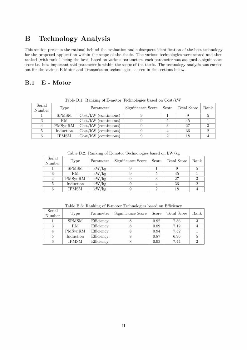
B Technology Analysis

This section presents the rational behind the evaluation and subsequent identification of the best technologyfor the proposed application within the scope of the thesis. The various technologies were scored and thenranked (with rank 1 being the best) based on various parameters, each parameter was assigned a significancescore i.e. how important said parameter is within the scope of the thesis. The technology analysis was carriedout for the various E-Motor and Transmission technologies as seen in the sections below.

B.1 E - Motor

Table B.1: Ranking of E-motor Technologies based on Cost/kWSerial

NumberType Parameter Significance Score Score Total Score Rank

1 SPMSM Cost/kW (continuous) 9 1 9 53 RM Cost/kW (continuous) 9 5 45 14 PMSynRM Cost/kW (continuous) 9 3 27 35 Induction Cost/kW (continuous) 9 4 36 26 IPMSM Cost/kW (continuous) 9 2 18 4

Table B.2: Ranking of E-motor Technologies based on kW/kgSerial

NumberType Parameter Significance Score Score Total Score Rank

1 SPMSM kW/kg 9 1 9 53 RM kW/kg 9 5 45 14 PMSynRM kW/kg 9 3 27 35 Induction kW/kg 9 4 36 26 IPMSM kW/kg 9 2 18 4

Table B.3: Ranking of E-motor Technologies based on EfficiencySerial

NumberType Parameter Significance Score Score Total Score Rank

1 SPMSM Efficiency 8 0.92 7.36 33 RM Efficiency 8 0.89 7.12 44 PMSynRM Efficiency 8 0.94 7.52 15 Induction Efficiency 8 0.87 6.96 56 IPMSM Efficiency 8 0.93 7.44 2

II

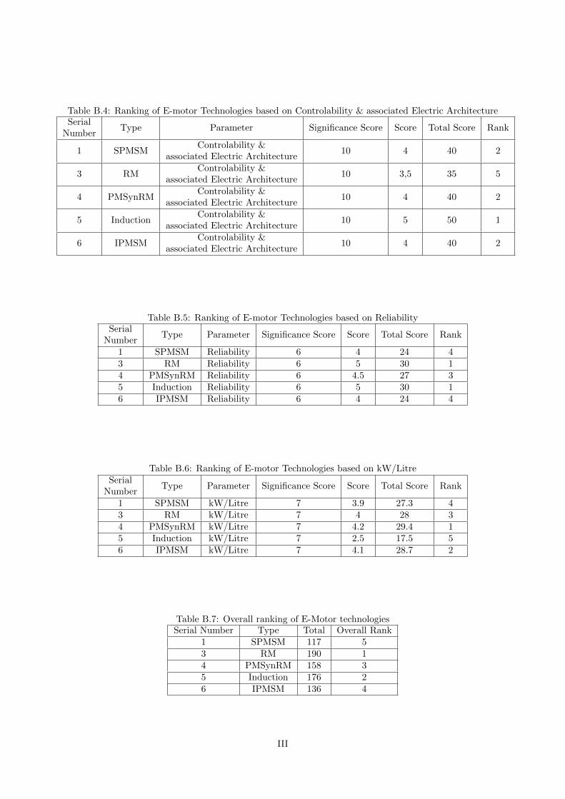
Table B.4: Ranking of E-motor Technologies based on Controlability & associated Electric ArchitectureSerial

NumberType Parameter Significance Score Score Total Score Rank

1 SPMSMControlability &

associated Electric Architecture10 4 40 2

3 RMControlability &

associated Electric Architecture10 3,5 35 5

4 PMSynRMControlability &

associated Electric Architecture10 4 40 2

5 InductionControlability &

associated Electric Architecture10 5 50 1

6 IPMSMControlability &

associated Electric Architecture10 4 40 2

Table B.5: Ranking of E-motor Technologies based on ReliabilitySerial

NumberType Parameter Significance Score Score Total Score Rank

1 SPMSM Reliability 6 4 24 43 RM Reliability 6 5 30 14 PMSynRM Reliability 6 4.5 27 35 Induction Reliability 6 5 30 16 IPMSM Reliability 6 4 24 4

Table B.6: Ranking of E-motor Technologies based on kW/LitreSerial

NumberType Parameter Significance Score Score Total Score Rank

1 SPMSM kW/Litre 7 3.9 27.3 43 RM kW/Litre 7 4 28 34 PMSynRM kW/Litre 7 4.2 29.4 15 Induction kW/Litre 7 2.5 17.5 56 IPMSM kW/Litre 7 4.1 28.7 2

Table B.7: Overall ranking of E-Motor technologiesSerial Number Type Total Overall Rank

1 SPMSM 117 53 RM 190 14 PMSynRM 158 35 Induction 176 26 IPMSM 136 4

III

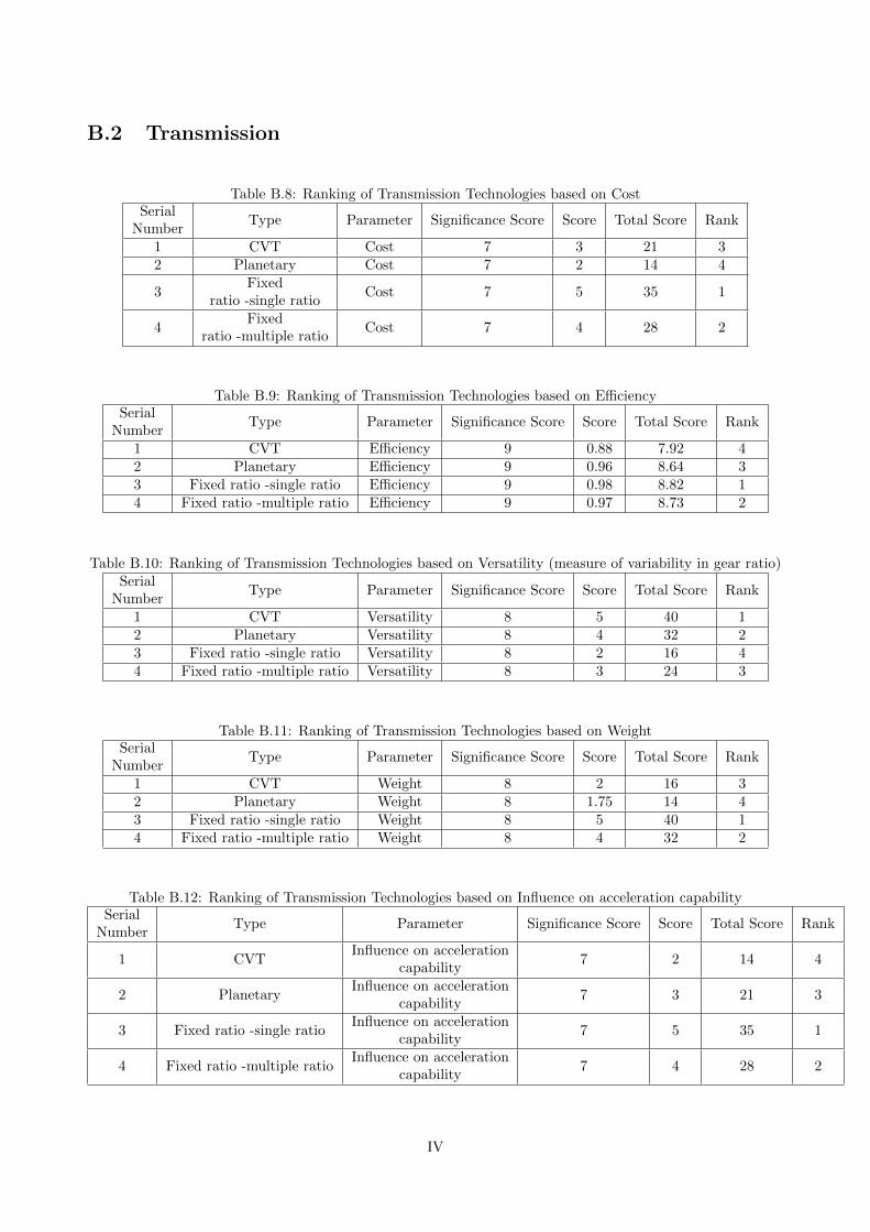
B.2 Transmission

Table B.8: Ranking of Transmission Technologies based on CostSerial

NumberType Parameter Significance Score Score Total Score Rank

1 CVT Cost 7 3 21 32 Planetary Cost 7 2 14 4

3Fixed

ratio -single ratioCost 7 5 35 1

4Fixed

ratio -multiple ratioCost 7 4 28 2

Table B.9: Ranking of Transmission Technologies based on EfficiencySerial

NumberType Parameter Significance Score Score Total Score Rank

1 CVT Efficiency 9 0.88 7.92 42 Planetary Efficiency 9 0.96 8.64 33 Fixed ratio -single ratio Efficiency 9 0.98 8.82 14 Fixed ratio -multiple ratio Efficiency 9 0.97 8.73 2

Table B.10: Ranking of Transmission Technologies based on Versatility (measure of variability in gear ratio)Serial

NumberType Parameter Significance Score Score Total Score Rank

1 CVT Versatility 8 5 40 12 Planetary Versatility 8 4 32 23 Fixed ratio -single ratio Versatility 8 2 16 44 Fixed ratio -multiple ratio Versatility 8 3 24 3

Table B.11: Ranking of Transmission Technologies based on WeightSerial

NumberType Parameter Significance Score Score Total Score Rank

1 CVT Weight 8 2 16 32 Planetary Weight 8 1.75 14 43 Fixed ratio -single ratio Weight 8 5 40 14 Fixed ratio -multiple ratio Weight 8 4 32 2

Table B.12: Ranking of Transmission Technologies based on Influence on acceleration capabilitySerial

NumberType Parameter Significance Score Score Total Score Rank

1 CVTInfluence on acceleration

capability7 2 14 4

2 PlanetaryInfluence on acceleration

capability7 3 21 3

3 Fixed ratio -single ratioInfluence on acceleration

capability7 5 35 1

4 Fixed ratio -multiple ratioInfluence on acceleration

capability7 4 28 2

IV

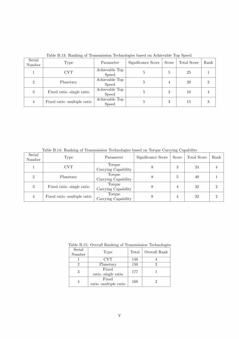
Table B.13: Ranking of Transmission Technologies based on Achievable Top SpeedSerial

NumberType Parameter Significance Score Score Total Score Rank

1 CVTAchievable Top

Speed5 5 25 1

2 PlanetaryAchievable Top

Speed5 4 20 2

3 Fixed ratio -single ratioAchievable Top

Speed5 2 10 4

4 Fixed ratio -multiple ratioAchievable Top

Speed5 3 15 3

Table B.14: Ranking of Transmission Technologies based on Torque Carrying CapabilitySerial

NumberType Parameter Significance Score Score Total Score Rank

1 CVTTorque

Carrying Capability8 3 24 4

2 PlanetaryTorque

Carrying Capability8 5 40 1

3 Fixed ratio -single ratioTorque

Carrying Capability8 4 32 2

4 Fixed ratio -multiple ratioTorque

Carrying Capability8 4 32 2

Table B.15: Overall Ranking of Transmission TechnologiesSerial

NumberType Total Overall Rank

1 CVT 148 42 Planetary 150 3

3Fixed

ratio -single ratio177 1

4Fixed

ratio -multiple ratio168 2

V

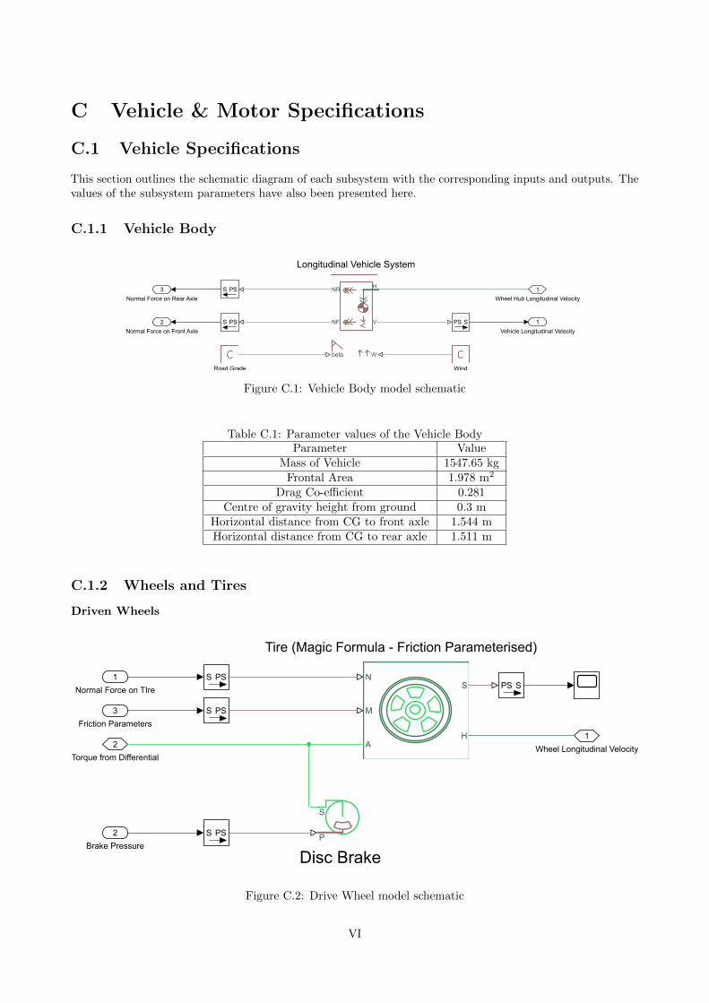
C Vehicle & Motor Specifications

C.1 Vehicle Specifications

This section outlines the schematic diagram of each subsystem with the corresponding inputs and outputs. Thevalues of the subsystem parameters have also been presented here.

C.1.1 Vehicle Body

LongitudinalVehicleSystem

SPS

WindRoadGrade

1VehicleLongitudinalVelocity

1WheelHubLongitudinalVelocity

S PS

S PS2NormalForceonFrontAxle

3NormalForceonRearAxle

Figure C.1: Vehicle Body model schematic

Table C.1: Parameter values of the Vehicle BodyParameter Value

Mass of Vehicle 1547.65 kgFrontal Area 1.978 m2

Drag Co-efficient 0.281Centre of gravity height from ground 0.3 m

Horizontal distance from CG to front axle 1.544 mHorizontal distance from CG to rear axle 1.511 m

C.1.2 Wheels and Tires

Driven Wheels

DiscBrake

Tire(MagicFormula-FrictionParameterised)

S PS1NormalForceonTIre

1WheelLongitudinalVelocity2

TorquefromDifferential

SPS

S PS2BrakePressure

3FrictionParameters

S PS

Figure C.2: Drive Wheel model schematic

VI

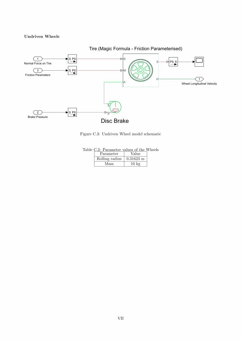
Undriven Wheels

DiscBrake

Tire(MagicFormula-FrictionParameterised)

S PS1NormalForceonTIre

1WheelLongitudinalVelocity

SPS

S PS2BrakePressure

3FrictionParameters

S PS

Figure C.3: Undriven Wheel model schematic

Table C.2: Parameter values of the WheelsParameter Value

Rolling radius 0.31623 mMass 10 kg

VII

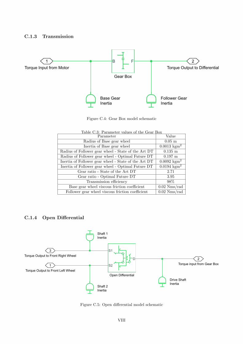
C.1.3 Transmission

GearBox

BaseGearInertia

FollowerGearInertia

1TorqueInputfromMotor

2TorqueOutputtoDifferential

Figure C.4: Gear Box model schematic

Table C.3: Parameter values of the Gear BoxParameter Value

Radius of Base gear wheel 0.05 mInertia of Base gear wheel 0.0013 kgm2

Radius of Follower gear wheel - State of the Art DT 0.135 mRadius of Follower gear wheel - Optimal Future DT 0.197 mInertia of Follower gear wheel - State of the Art DT 0.0092 kgm2

Inertia of Follower gear wheel - Optimal Future DT 0.0194 kgm2

Gear ratio - State of the Art DT 2.71Gear ratio - Optimal Future DT 3.95

Transmission efficiency 98%Base gear wheel viscous friction coefficient 0.02 Nms/rad

Follower gear wheel viscous friction coefficient 0.02 Nms/rad

C.1.4 Open Differential

1TorqueOutputtoFrontLeftWheel

2TorqueinputfromGearBox

3TorqueOutputtoFrontRightWheel

DriveShaftInertia

Shaft1Inertia

Shaft2Inertia

OpenDifferential

Figure C.5: Open differential model schematic

VIII

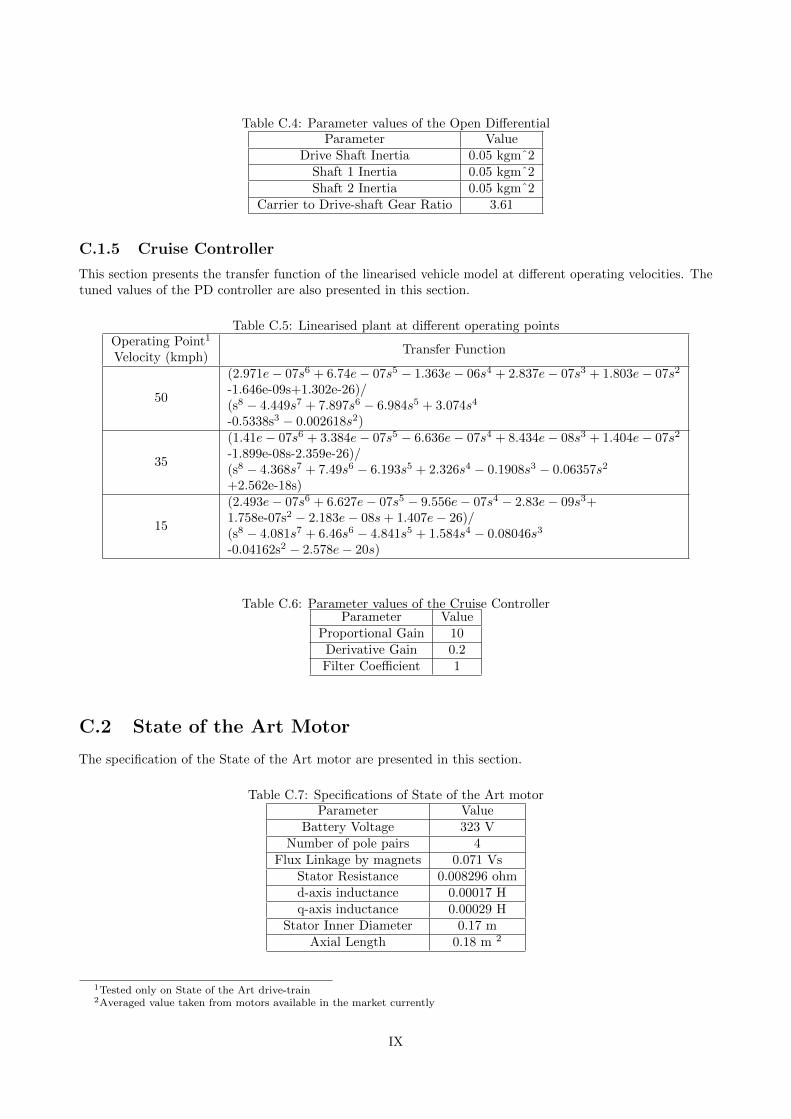
Table C.4: Parameter values of the Open DifferentialParameter Value

Drive Shaft Inertia 0.05 kgmˆ2Shaft 1 Inertia 0.05 kgmˆ2Shaft 2 Inertia 0.05 kgmˆ2

Carrier to Drive-shaft Gear Ratio 3.61

C.1.5 Cruise Controller

This section presents the transfer function of the linearised vehicle model at different operating velocities. Thetuned values of the PD controller are also presented in this section.

Table C.5: Linearised plant at different operating pointsOperating Point1

Velocity (kmph)Transfer Function

50

(2.971e− 07s6 + 6.74e− 07s5 − 1.363e− 06s4 + 2.837e− 07s3 + 1.803e− 07s2

-1.646e-09s+1.302e-26)/(s8 − 4.449s7 + 7.897s6 − 6.984s5 + 3.074s4

-0.5338s3 − 0.002618s2)

35

(1.41e− 07s6 + 3.384e− 07s5 − 6.636e− 07s4 + 8.434e− 08s3 + 1.404e− 07s2

-1.899e-08s-2.359e-26)/(s8 − 4.368s7 + 7.49s6 − 6.193s5 + 2.326s4 − 0.1908s3 − 0.06357s2

+2.562e-18s)

15

(2.493e− 07s6 + 6.627e− 07s5 − 9.556e− 07s4 − 2.83e− 09s3+1.758e-07s2 − 2.183e− 08s+ 1.407e− 26)/(s8 − 4.081s7 + 6.46s6 − 4.841s5 + 1.584s4 − 0.08046s3

-0.04162s2 − 2.578e− 20s)

Table C.6: Parameter values of the Cruise ControllerParameter Value

Proportional Gain 10Derivative Gain 0.2Filter Coefficient 1

C.2 State of the Art Motor

The specification of the State of the Art motor are presented in this section.

Table C.7: Specifications of State of the Art motorParameter Value

Battery Voltage 323 VNumber of pole pairs 4

Flux Linkage by magnets 0.071 VsStator Resistance 0.008296 ohmd-axis inductance 0.00017 Hq-axis inductance 0.00029 H

Stator Inner Diameter 0.17 mAxial Length 0.18 m 2

1Tested only on State of the Art drive-train2Averaged value taken from motors available in the market currently

IX

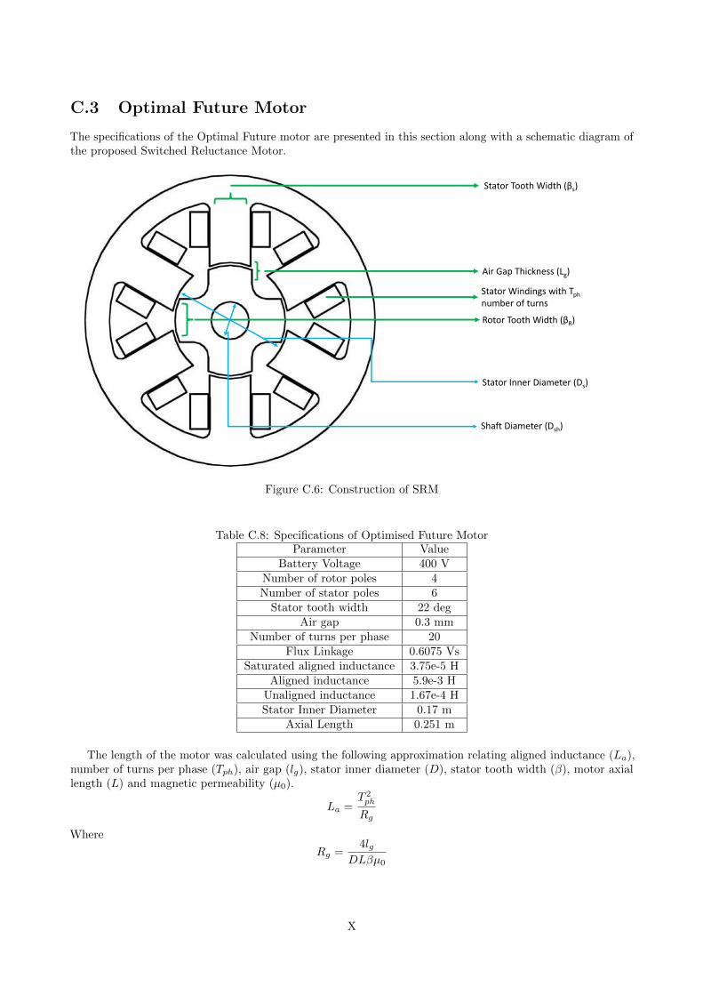
C.3 Optimal Future Motor

The specifications of the Optimal Future motor are presented in this section along with a schematic diagram ofthe proposed Switched Reluctance Motor.

Stator Tooth Width (βs)

Rotor Tooth Width (βR)

Air Gap Thickness (Lg)

Stator Windings with Tph

number of turns

Stator Inner Diameter (Ds)

Shaft Diameter (Dsh)

Figure C.6: Construction of SRM

Table C.8: Specifications of Optimised Future MotorParameter Value

Battery Voltage 400 VNumber of rotor poles 4Number of stator poles 6

Stator tooth width 22 degAir gap 0.3 mm

Number of turns per phase 20Flux Linkage 0.6075 Vs

Saturated aligned inductance 3.75e-5 HAligned inductance 5.9e-3 H

Unaligned inductance 1.67e-4 HStator Inner Diameter 0.17 m

Axial Length 0.251 m

The length of the motor was calculated using the following approximation relating aligned inductance (La),number of turns per phase (Tph), air gap (lg), stator inner diameter (D), stator tooth width (β), motor axiallength (L) and magnetic permeability (µ0).

La =T 2ph

Rg

Where

Rg =4lg

DLβµ0

X

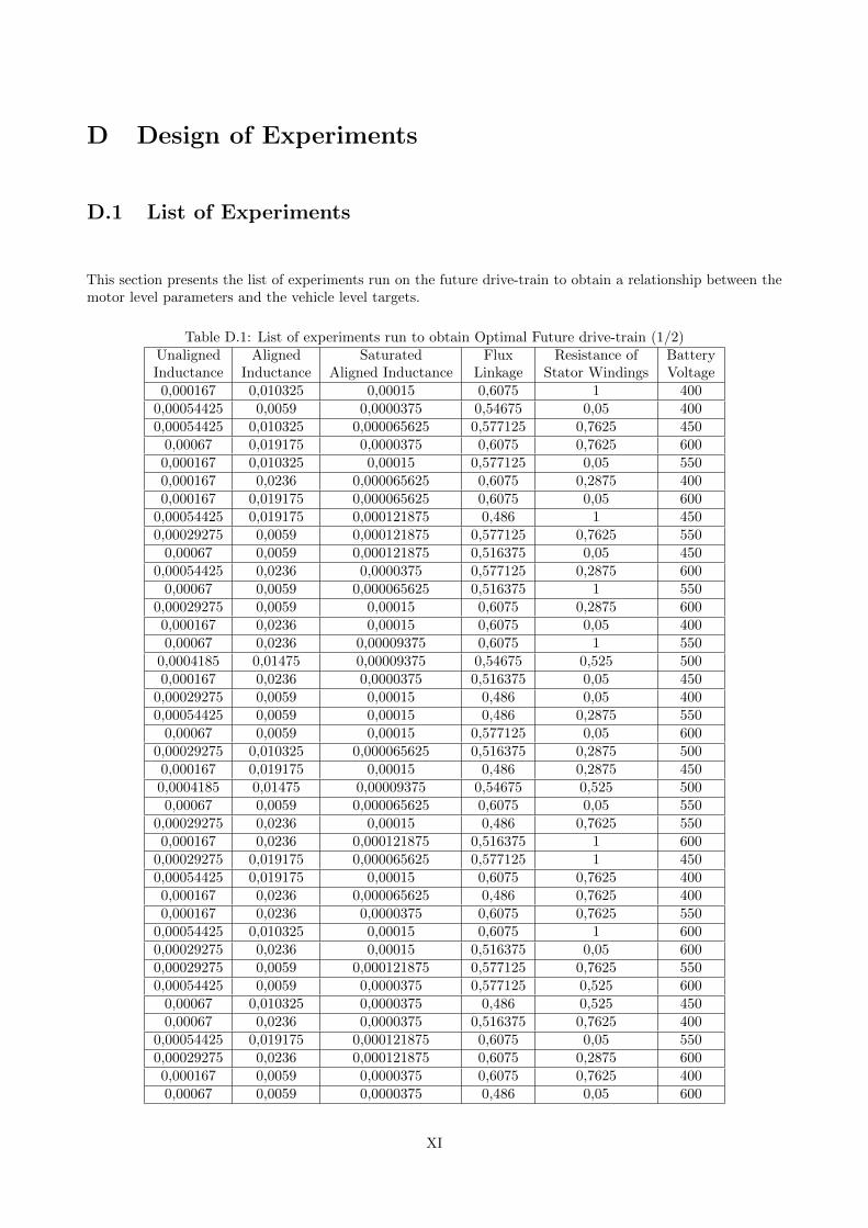
D Design of Experiments

D.1 List of Experiments

This section presents the list of experiments run on the future drive-train to obtain a relationship between themotor level parameters and the vehicle level targets.

Table D.1: List of experiments run to obtain Optimal Future drive-train (1/2)UnalignedInductance

AlignedInductance

SaturatedAligned Inductance

FluxLinkage

Resistance ofStator Windings

BatteryVoltage

0,000167 0,010325 0,00015 0,6075 1 4000,00054425 0,0059 0,0000375 0,54675 0,05 4000,00054425 0,010325 0,000065625 0,577125 0,7625 450

0,00067 0,019175 0,0000375 0,6075 0,7625 6000,000167 0,010325 0,00015 0,577125 0,05 5500,000167 0,0236 0,000065625 0,6075 0,2875 4000,000167 0,019175 0,000065625 0,6075 0,05 600

0,00054425 0,019175 0,000121875 0,486 1 4500,00029275 0,0059 0,000121875 0,577125 0,7625 550

0,00067 0,0059 0,000121875 0,516375 0,05 4500,00054425 0,0236 0,0000375 0,577125 0,2875 600

0,00067 0,0059 0,000065625 0,516375 1 5500,00029275 0,0059 0,00015 0,6075 0,2875 6000,000167 0,0236 0,00015 0,6075 0,05 4000,00067 0,0236 0,00009375 0,6075 1 550

0,0004185 0,01475 0,00009375 0,54675 0,525 5000,000167 0,0236 0,0000375 0,516375 0,05 450

0,00029275 0,0059 0,00015 0,486 0,05 4000,00054425 0,0059 0,00015 0,486 0,2875 550

0,00067 0,0059 0,00015 0,577125 0,05 6000,00029275 0,010325 0,000065625 0,516375 0,2875 5000,000167 0,019175 0,00015 0,486 0,2875 4500,0004185 0,01475 0,00009375 0,54675 0,525 5000,00067 0,0059 0,000065625 0,6075 0,05 550

0,00029275 0,0236 0,00015 0,486 0,7625 5500,000167 0,0236 0,000121875 0,516375 1 600

0,00029275 0,019175 0,000065625 0,577125 1 4500,00054425 0,019175 0,00015 0,6075 0,7625 4000,000167 0,0236 0,000065625 0,486 0,7625 4000,000167 0,0236 0,0000375 0,6075 0,7625 550

0,00054425 0,010325 0,00015 0,6075 1 6000,00029275 0,0236 0,00015 0,516375 0,05 6000,00029275 0,0059 0,000121875 0,577125 0,7625 5500,00054425 0,0059 0,0000375 0,577125 0,525 600

0,00067 0,010325 0,0000375 0,486 0,525 4500,00067 0,0236 0,0000375 0,516375 0,7625 400

0,00054425 0,019175 0,000121875 0,6075 0,05 5500,00029275 0,0236 0,000121875 0,6075 0,2875 6000,000167 0,0059 0,0000375 0,6075 0,7625 4000,00067 0,0059 0,0000375 0,486 0,05 600

XI

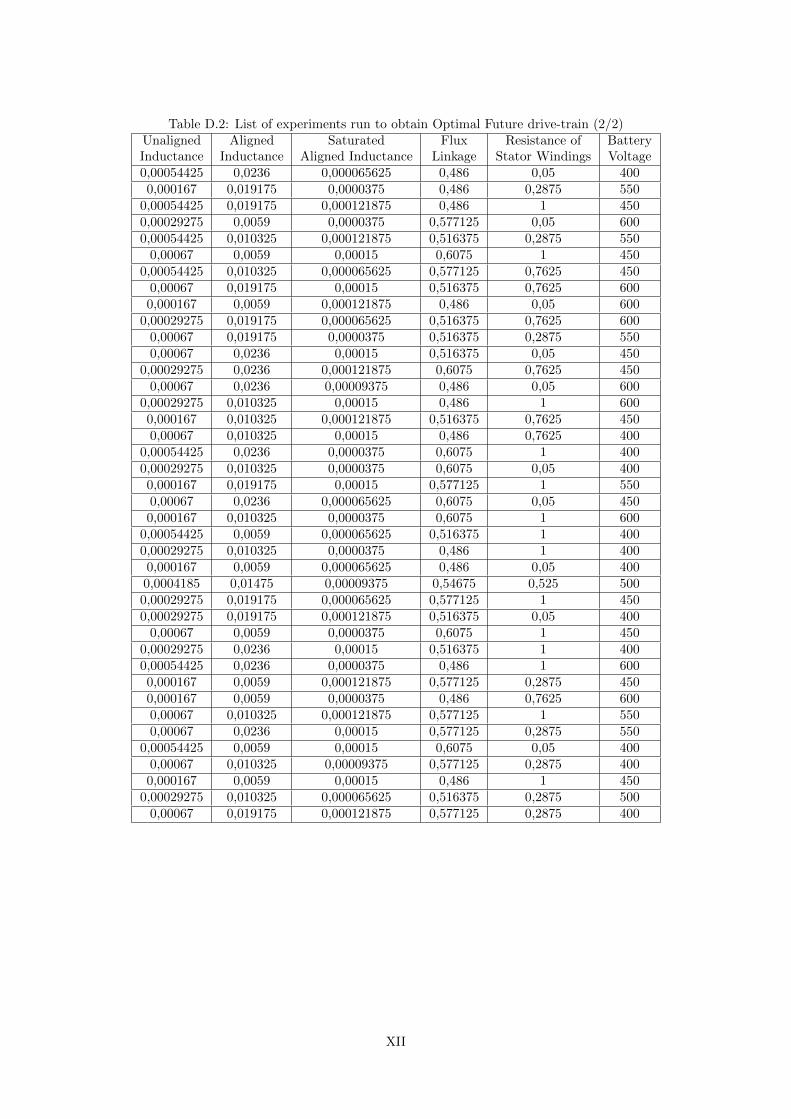
Table D.2: List of experiments run to obtain Optimal Future drive-train (2/2)UnalignedInductance

AlignedInductance

SaturatedAligned Inductance

FluxLinkage

Resistance ofStator Windings

BatteryVoltage

0,00054425 0,0236 0,000065625 0,486 0,05 4000,000167 0,019175 0,0000375 0,486 0,2875 550

0,00054425 0,019175 0,000121875 0,486 1 4500,00029275 0,0059 0,0000375 0,577125 0,05 6000,00054425 0,010325 0,000121875 0,516375 0,2875 550

0,00067 0,0059 0,00015 0,6075 1 4500,00054425 0,010325 0,000065625 0,577125 0,7625 450

0,00067 0,019175 0,00015 0,516375 0,7625 6000,000167 0,0059 0,000121875 0,486 0,05 600

0,00029275 0,019175 0,000065625 0,516375 0,7625 6000,00067 0,019175 0,0000375 0,516375 0,2875 5500,00067 0,0236 0,00015 0,516375 0,05 450

0,00029275 0,0236 0,000121875 0,6075 0,7625 4500,00067 0,0236 0,00009375 0,486 0,05 600

0,00029275 0,010325 0,00015 0,486 1 6000,000167 0,010325 0,000121875 0,516375 0,7625 4500,00067 0,010325 0,00015 0,486 0,7625 400

0,00054425 0,0236 0,0000375 0,6075 1 4000,00029275 0,010325 0,0000375 0,6075 0,05 4000,000167 0,019175 0,00015 0,577125 1 5500,00067 0,0236 0,000065625 0,6075 0,05 4500,000167 0,010325 0,0000375 0,6075 1 600

0,00054425 0,0059 0,000065625 0,516375 1 4000,00029275 0,010325 0,0000375 0,486 1 4000,000167 0,0059 0,000065625 0,486 0,05 4000,0004185 0,01475 0,00009375 0,54675 0,525 5000,00029275 0,019175 0,000065625 0,577125 1 4500,00029275 0,019175 0,000121875 0,516375 0,05 400

0,00067 0,0059 0,0000375 0,6075 1 4500,00029275 0,0236 0,00015 0,516375 1 4000,00054425 0,0236 0,0000375 0,486 1 6000,000167 0,0059 0,000121875 0,577125 0,2875 4500,000167 0,0059 0,0000375 0,486 0,7625 6000,00067 0,010325 0,000121875 0,577125 1 5500,00067 0,0236 0,00015 0,577125 0,2875 550

0,00054425 0,0059 0,00015 0,6075 0,05 4000,00067 0,010325 0,00009375 0,577125 0,2875 4000,000167 0,0059 0,00015 0,486 1 450

0,00029275 0,010325 0,000065625 0,516375 0,2875 5000,00067 0,019175 0,000121875 0,577125 0,2875 400

XII

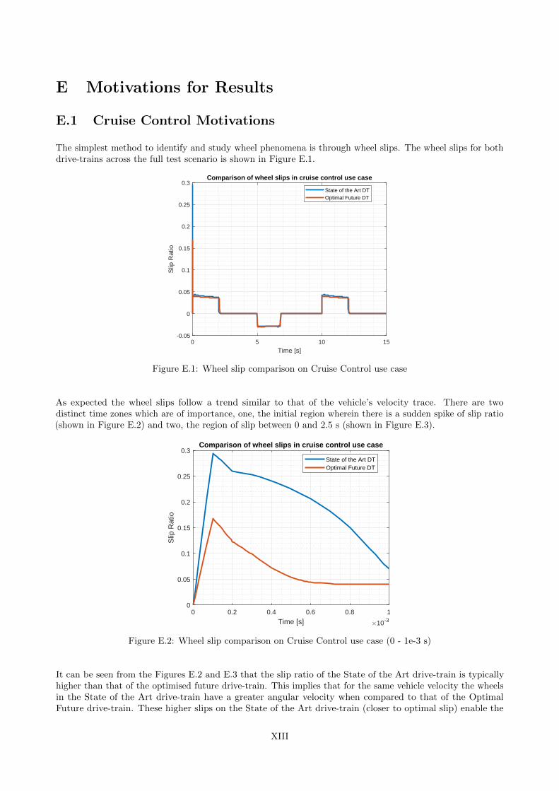
E Motivations for Results

E.1 Cruise Control Motivations

The simplest method to identify and study wheel phenomena is through wheel slips. The wheel slips for bothdrive-trains across the full test scenario is shown in Figure E.1.

0 5 10 15

Time [s]

-0.05

0

0.05

0.1

0.15

0.2

0.25

0.3

Slip

Rat

ioComparison of wheel slips in cruise control use case

State of the Art DTOptimal Future DT

Figure E.1: Wheel slip comparison on Cruise Control use case

As expected the wheel slips follow a trend similar to that of the vehicle’s velocity trace. There are twodistinct time zones which are of importance, one, the initial region wherein there is a sudden spike of slip ratio(shown in Figure E.2) and two, the region of slip between 0 and 2.5 s (shown in Figure E.3).

0 0.2 0.4 0.6 0.8 1

Time [s] 10-3

0

0.05

0.1

0.15

0.2

0.25

0.3

Slip

Rat

io

Comparison of wheel slips in cruise control use case

State of the Art DTOptimal Future DT

Figure E.2: Wheel slip comparison on Cruise Control use case (0 - 1e-3 s)

It can be seen from the Figures E.2 and E.3 that the slip ratio of the State of the Art drive-train is typicallyhigher than that of the optimised future drive-train. This implies that for the same vehicle velocity the wheelsin the State of the Art drive-train have a greater angular velocity when compared to that of the OptimalFuture drive-train. These higher slips on the State of the Art drive-train (closer to optimal slip) enable the

XIII

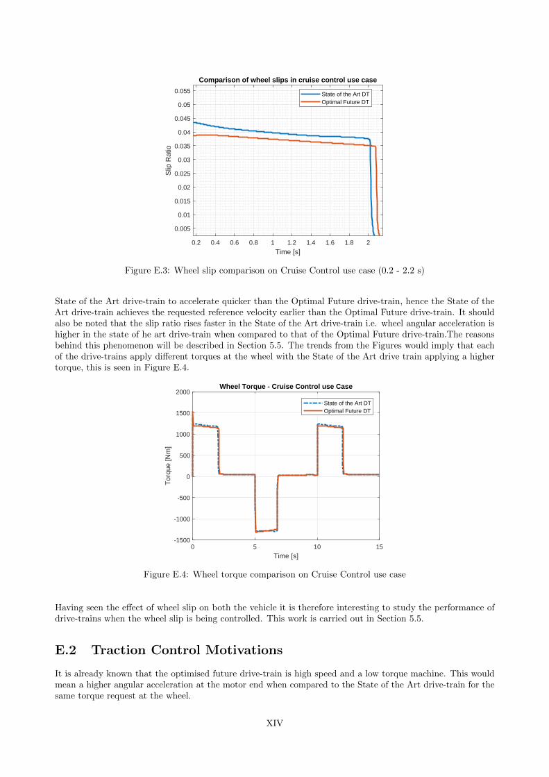
0.2 0.4 0.6 0.8 1 1.2 1.4 1.6 1.8 2

Time [s]

0.005

0.01

0.015

0.02

0.025

0.03

0.035

0.04

0.045

0.05

0.055

Slip

Rat

io

Comparison of wheel slips in cruise control use case

State of the Art DTOptimal Future DT

Figure E.3: Wheel slip comparison on Cruise Control use case (0.2 - 2.2 s)

State of the Art drive-train to accelerate quicker than the Optimal Future drive-train, hence the State of theArt drive-train achieves the requested reference velocity earlier than the Optimal Future drive-train. It shouldalso be noted that the slip ratio rises faster in the State of the Art drive-train i.e. wheel angular acceleration ishigher in the state of he art drive-train when compared to that of the Optimal Future drive-train.The reasonsbehind this phenomenon will be described in Section 5.5. The trends from the Figures would imply that eachof the drive-trains apply different torques at the wheel with the State of the Art drive train applying a highertorque, this is seen in Figure E.4.

0 5 10 15

Time [s]

-1500

-1000

-500

0

500

1000

1500

2000

Tor

que

[Nm

]

Wheel Torque - Cruise Control use Case

State of the Art DTOptimal Future DT

Figure E.4: Wheel torque comparison on Cruise Control use case

Having seen the effect of wheel slip on both the vehicle it is therefore interesting to study the performance ofdrive-trains when the wheel slip is being controlled. This work is carried out in Section 5.5.

E.2 Traction Control Motivations

It is already known that the optimised future drive-train is high speed and a low torque machine. This wouldmean a higher angular acceleration at the motor end when compared to the State of the Art drive-train for thesame torque request at the wheel.

XIV

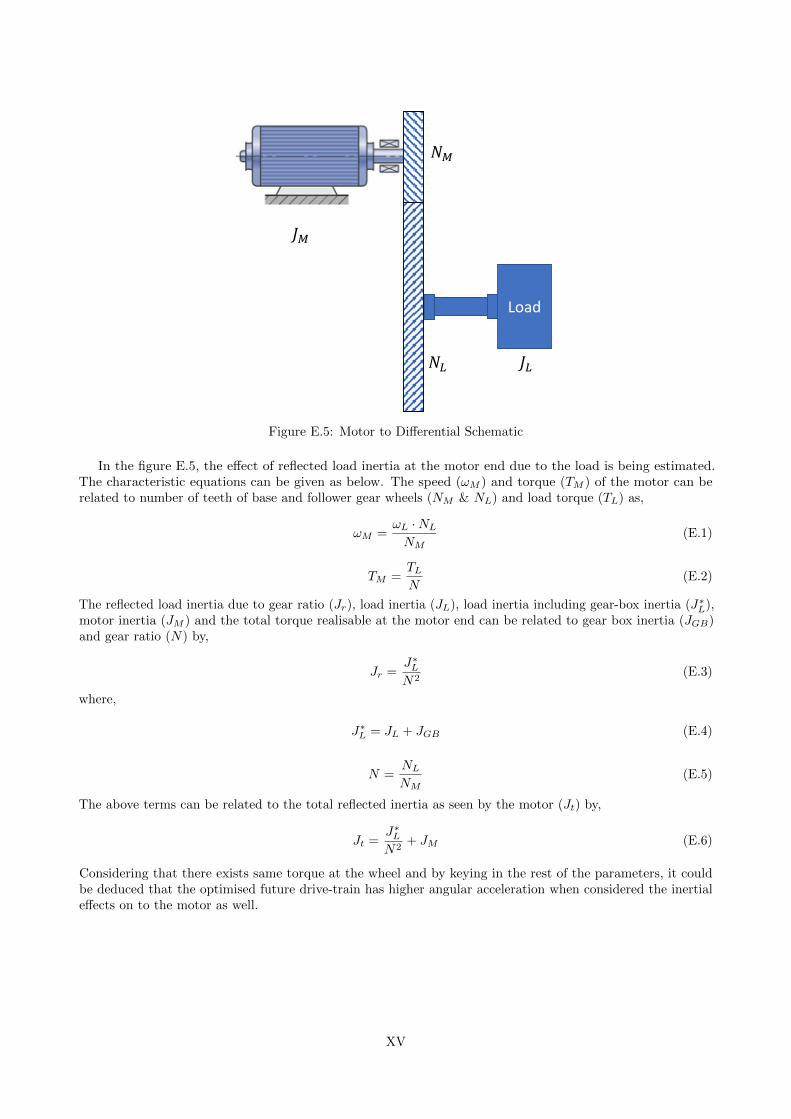
Load

𝐽𝑀

𝑁𝑀

𝑁𝐿 𝐽𝐿

Figure E.5: Motor to Differential Schematic

In the figure E.5, the effect of reflected load inertia at the motor end due to the load is being estimated.The characteristic equations can be given as below. The speed (ωM ) and torque (TM ) of the motor can berelated to number of teeth of base and follower gear wheels (NM & NL) and load torque (TL) as,

ωM =ωL ·NL

NM(E.1)

TM =TLN

(E.2)

The reflected load inertia due to gear ratio (Jr), load inertia (JL), load inertia including gear-box inertia (J∗L),

motor inertia (JM ) and the total torque realisable at the motor end can be related to gear box inertia (JGB)and gear ratio (N) by,

Jr =J∗L

N2(E.3)

where,

J∗L = JL + JGB (E.4)

N =NL

NM(E.5)

The above terms can be related to the total reflected inertia as seen by the motor (Jt) by,

Jt =J∗L

N2+ JM (E.6)

Considering that there exists same torque at the wheel and by keying in the rest of the parameters, it couldbe deduced that the optimised future drive-train has higher angular acceleration when considered the inertialeffects on to the motor as well.

XV