Propulsion solutions for the cruise industry: A comparison between conventional

shaftline propulsion and Azipod® propulsion.

Master of Science Thesis Douglas L. Frongillo Department of Shipping and Marine Technology CHALMERS UNIVERSITY OF TECHNOLOGY Göteborg, Sweden, 2011 Report No. X-11/269

A THESIS FOR THE DEGREE OF MASTER OF SCIENCE Propulsion solutions for the cruise industry: A comparison between conventional shaftline propulsion and Azipod® propulsion. DOUGLAS L. FRONGILLO

Department of Shipping and Marine Technology CHALMERS UNIVERSITY OF TECHNOLOGY Göteborg, Sweden 2011

Propulsion solutions for the cruise industry: A comparison between conventional shaftline propulsion and Azipod® propulsion. DOUGLAS L. FRONGILLO © DOUGLAS L. FRONGILLO, 2011 Report No. X-11/269 Department of Shipping and Marine Technology Chalmers University of Technology SE-412 96 Göteborg Sweden Telephone +46 (0)31-772 1000 Printed by Chalmers Reproservice Göteborg, Sweden, 2011

A THESIS FOR THE DEGREE OF MASTER OF SCIENCE Propulsion solutions for the cruise industry: A comparison between conventional shaftline propulsion and Azipod® propulsion. DOUGLAS L. FRONGILLO Department of Shipping and Marine Technology Chalmers University of Technology

Abstract The rise in cost of marine fuels has forced ship owners and operators to evaluate current operational practices and efficiency losses onboard for potential cost savings. Although there are substantial savings to be made through operational changes, this study focuses on the recovery of lost efficiency through propulsion machinery optimization. Focusing on life time cost analysis as opposed to capital expenditure for initial outfitting can outline a larger potential for savings than that seen when directly comparing building costs. This study was completed to determine the overall difference in propulsion efficiency between conventional shaftline propulsion and AZIPOD® propulsion using computational fluid dynamics (CFD). The viscous CFD calculations were conducted with the commercial RANSE code; STAR-CCM+ Ver 6.02.009.

STAR-CCM+ is a finite volume code, which solves the unsteady Reynolds-Averaged Navier-Stokes equations together with the continuity equation in integral form. In order to include viscous effects in the simulation, turbulence modeling is required. For the present application the two-equation, k-ω model with an All-Y+ treatment was applied. Free surface effects were included in the simulation, and were modeled using a flat Volume of Fluid (VOF) wave along with a two-phase Eulerian Multi-phase and Multi-phase Equation of State model. The Eulerian phases were defined as an Air-Seawater interface at 20°C. Dynamic motions of the vessel were not modeled during the simulation. The simulation was set up as a self-propulsion simulation with a momentum source applied to model propeller action. Results clearly indicate a savings in propulsion efficiency when the AZIPOD® option is applied.

[-] [m][-Aft] [N] [kW] [-] [kW]

Sim # Trim RTS PE ηo PD

POD 304.2A 0.000 1.81E+06 22167 0.701 31622

SHAFT 304.2 0.000 1.98E+06 24346 0.670 36337

Table A-1

The solutions show considerable differences in drag, attributed to the increase in turbulence around the shaftline and brackets and the increase of approximately 1.4% in wetted surface area on the shaftline vessel.

1

No propeller geometry or propeller curves were available for this study, leading to the implementation of the momentum source model to provide the pressure/velocity gradient across the propeller disc region necessary to simulate the propeller induced drag present on the appendages in the propeller wake. Results could be improved in terms of absolute values by running the simulations at full scale with surface roughness height defined according to actual clean hull condition, activation of a motion solver to simulate dynamic forces acting of on the flaoting body, and substitution of the momentum source model with the actual propeller geometry so that propeller hull interaction is captured as well as the correct propeller wake.

2

Preface This thesis is a part of the requirements for the master’s degree at Chalmers University of Technology, Göteborg, and has been carried out at the Department of Shipping and Marine Technology, Chalmers University of Technology. I would like to acknowledge and thank my examiner and supervisor, Associate Professor Rickard Bensow at the Department of Shipping and Marine Technology, for his assistance and guidance during the development of this study. I would also like to thank Mr. Christer Karlsson of Norwegian Cruise Line Newbuilding Dept., Mr. Finn Wollesen of Knud E. Hansen A/S, Mr. Lars Danielsson, Mr. Henning Luhmann of Meyer Werft Shipyard, and Mr. Tomi Vikenheimo of ABB for their various contributions throughout this study. Göteborg, June, 2011 Douglas L. Frongillo

3

Contents

Abstract --------------------------------------------------------------------------------------------------- 1

Preface ---------------------------------------------------------------------------------------------------- 3

Contents -------------------------------------------------------------------------------------------------- 4

1. Introduction ------------------------------------------------------------------------------------------- 6

1.1. Background --------------------------------------------------------------------------------------- 6

1.2. Objective with the investigation --------------------------------------------------------------- 7

1.3. Methodology ------------------------------------------------------------------------------------- 7

2. Literature Review ------------------------------------------------------------------------------------ 8

2.1 Summary -------------------------------------------------------------------------------------- 9

3. Methodology ------------------------------------------------------------------------------------------ 9

4. Solution Strategy ------------------------------------------------------------------------------------ 10

4.1 Assumptions and Simplifications -------------------------------------------------------------- 12

4.2 Geometry and Mesh Continua ----------------------------------------------------------------- 12

4.3 Physics Continua -------------------------------------------------------------------------------- 16

4.3.1 Physics Models -------------------------------------------------------------------------- 16

4.3.2 Governing Equations -------------------------------------------------------------------- 17

4.3.3 Reference Values ------------------------------------------------------------------------ 18

4.3.4 Initial Conditions ------------------------------------------------------------------------ 18

4.4 Boundary Conditions ---------------------------------------------------------------------------- 19

4.4.1 Inlet Boundaries ------------------------------------------------------------------------- 19

4.4.2 Symmetry Boundaries ------------------------------------------------------------------ 19

4.4.3 Outlet Boundaries ----------------------------------------------------------------------- 20

4.4.4 Region Settings -------------------------------------------------------------------------- 20

4.4.5 Momentum Source Model -------------------------------------------------------------- 20

4.5 Solver --------------------------------------------------------------------------------------------- 21

5. Results ------------------------------------------------------------------------------------------------- 22

6. Conclusion -------------------------------------------------------------------------------------------- 35

9. References -------------------------------------------------------------------------------------------- 36

4

5

1. Introduction 1.1. Background

ABB introduced the Azipod® propulsion unit in 1989 with the first prototype installation, opening up new possibilities and flexibilities in propulsion drive systems onboard ship. The first cruise vessel installation followed in 1995 onboard the Carnival Elation. The marine industry recognized this as a significant step forward in propulsion and maneuvering technology. Soon more equipment manufacturers introduced their own solutions based on the Azipod® design. The arrival of the Azipod®introduced improved hydrodynamic efficiency, and the availability of maximum thrust in any direction. In addition to the main advantages previously described, the Azipod®also introduce technical complexity and higher investment cost. Due to this, the choice of Azipod® units as a main propulsion solution has been a controversial topic among ship-owners for more than two decades, and has remained largely in vessels requiring a higher technical complexity. Larger installations brought focus to issues outside of cost and efficiency, including dry-docking frequency, and operational limitations. It is the purpose of this thesis to investigate the long term financial commitments associated with selection of Azipods® as a propulsion option when compared to conventional shafting.

6

1.2. Objective with the investigation

The scope of this thesis study is to evaluate Azipod propulsion with conventional shaftline propulsion in terms of total resistance using CFD in order to predict operational cost savings. It is the intent that the forecasted savings can be used to determine if the increased capital and maintenance costs associated with Azipods®can be offset by the operational savings. 1.3. Methodology

This thesis will apply a commercial Finite Volume Computational Fluid Dynamics (CFD) code to estimate total resistance on hull and appendages. Aerodynamic drag will be limited to the geometry of the model, which focuses on the hull and does not take into consideration superstructure. This has been done for the sake of solver efficiency, and is assumed to be equal in both simulations. A momentum source model will be used to model propeller effects. Two (2) geometrically similar hulls will be evaluated, one (1) equipped with Azipod® propulsion, and one (1) equipped with conventional shaft line propulsion. In order to ensure geometrical similarity, the hull model chosen will be the same for each propulsion type, the only difference being the substitution of propulsion appendages. The hull chosen for this simulation has been supplied by Meyer Werft Shipyard, in cooperation with Norwegian Cruise Line, and is consistent with the Norwegian Jewel, hull No. 667.

7

2. Literature Review There is a large body of work available regarding CFD usage in ship hydrodynamics spanning more than three decades. The articles discussed below may differ slightly from the work completed in this thesis, however they share similar origins and discuss the validity and accuracy of transient calculations completed in model scale CFD. B. Bucan, P. Buca, and S. Ruzic [2008] completed a study of a VLCC to determine the accuracy of numerical simulations when compared to model experiments for large displacement vessels. A commercial CFD code Star CCM+ was used for numerical simulation of the VLCC in two (2) operational conditions, Ballast Condition and Fully Laden Condition (design condition). The model was not released for dynamic movement. The study was setup using the SIMPLE algorithm (an implicit scheme), and used the Star CCM+ segregated, algebraic multi-grid solver. The Mentor SST k-w Turbulence Model was used for near wall predictions with all y+ wall treatment, and a Volume of Fluid (VOF) model was used to model the free-surface and evaluate the interface between the fluid phases. Flow is governed with Reynolds Averaged Navier-Stokes Equations (RANSE). In the results, limiting streamlines plots for the numerical models are consistent with the results recorded from the physical model experiments. This also holds true for the free-surface elevation and wave patterns. The results for total resistance coefficients (CT) are within 1.3% and 2.1% for Ballast Condition and Design Condition respectively when compared to measured results. The wake field was plotted for both conditions with an over-lay of measured results to show the consistency of shape in regards to the axial velocity component. Physical similarities are apparent between the physical and numerical experiments. D Jürgens and M Palm, of Voith Turbo Schneider Propulsion GmbH & Co. in cooperation with M Periç and E Schreck, of CD-Adapco [2008] completed a series of studies to determine the accuracy of commercial CFD when compared to physical model testing when dynamic motions are considered. A similar approach to Bucan, Buca, and Ruzic was used for the numerical model setup, with the addition of the 6-DOF solver for prediction of hydrodynamic motions, and an extension of the study to also simulate using both the k-e Turbulence Model and k-w Turbulence Model. Two cases of interest in this study were: Towing Simulation of a Brick, focusing on the movement of a brick shaped bluff geometry with extreme motions in heave in pitch. In this simulation a hexahedral mesh was used. The results show that the predicted free-surface developed reasonably, however the floating position of the vessel was not as accurate. Towing Simulation of Tugboat , a virtual towing simulation for a tug boat fixed even keel with no dynamic motions was completed, and compared with a simulation using the same model setup released for heave and pitch motions.

8

In this simulation, a hexahedral mesh was used. The results show that a substantial under prediction of resistance is present when the vessel is fixed, however the results when the vessel is released are very consistent with physical experiments. The results of this study focus on the importance of mesh density and refinement when using motion solvers. Depending on the motion solver selected for the simulation, and the severity of motions, lack of refinement along the fluid interface can result in inaccuracy. 2.1 Summary

An understanding of the expected motions and choice of motion solver is extremely important in the setup of the mesh and boundary conditions. As motion solvers vary greatly, in function and application, an improperly resolved mesh can lead to unreliable results. This is especially important to simulations which cannot be compared to physical model tests. The k-w Turbulence Model is commonly used in marine hydrodynamic studies and demonstrates consistency and stability when used in fixed geometry simulations. The k-e Turbulence Model is also widely used, and has been argued to be a more suitable model when simulating dynamic motions. This can be due to lower sensitivity to mesh structure and refinement when considering mesh structure changes when using DFBI (dynamic fluid-body interaction) solvers, or sliding mesh models.

3. Methodology The use of CFD in prediction of ship hydrodynamics provides designers and researchers with additional tools for evaluation and visualization of complex flows and motions related to ship hydrodynamics. Many commercial CFD solvers have evolved to include advanced Graphic User Interfaces (GUIs), and explicit solver guidelines to open up CFD use to a larger group of engineers and designers who would otherwise not be able to use CFD as a design tool. The CFD process can be broken up into three distinct steps; Pre-Processing, Solving, and Post-Processing. Pre-processing includes the following steps;

Geometrical definition; CAD modeling and identification of domain constraints. Mesh generation Selection of physics to be modeled Fluid property definition Definition of boundary conditions

Meshing strategy is very important both for quality of result and solver efficiency. Advancements in CFD tools have allowed for semi-automated meshing processes to reduce the overall time associated with meshing and allow the user to arrive at a suitable mesh in less time, and devote more time to solving and post processing.

9

The Solver calculates the governing Navier-Stokes equations for transport, continuity and conservation of mass and energy for each node in the mesh contained within the computational domain for a time scale larger than the turbulent time scale. In most cases this does not yield results accurate enough for time-accurate solutions where complex turbulent properties are governing. All though not time accurate, the results reflect mean flow values, which in most cases are sufficient for power prediction, hull optimization and motion analysis when considering ship hydrodynamics. For more complex analysis regarding complex turbulent flows, and cavitation, further refinement of solver and mesh settings are required in order to arrive at a suitable result for a smaller time scale. When modeling ship hydrodynamics, Star CCM+ recommends the use of the segregated solver, as this performs well for constant density fluid flow conditions where flow is incompressible with low Mach numbers. For this approach, the solver solves the flow equations for each component of velocity and pressure separately and uses an iterative method to calculate the momentum and continuity equations. Star CCM+ uses a Rhie-Chow type pressure velocity coupling combined with the SIMPLE type algorithm for its segregated flow model. Star-CCM+ employs an Algebraic Multigrid Solver (AMG) for solving the discrete linear system iteratively. This is a guess-and-correct approach used for solving the pressure and velocity components used in calculating the momentum and continuity equations as discussed above. Although fairly robust and adaptable, the AMG solver does have its limitations when considering solver efficiency and convergence. The AMG solver is best used in coarser applications, where high or extreme fluctuations are removed quite quickly for the solution as it updates. The AMG does have a problem however with removing error as residuals decrease, making convergence slower at times where more refined mesh is used.

4. Solution Strategy The simulations were carried out in model scale. This is a widely used method as it is more computationally efficient then full scale simulating, and is directly comparable to model test results when available. The model scale used for this study is λ = 25.108. The results are ultimately extrapolated to full scale according to ITTC 1978, for the benefit of the owner. The solver setup chosen was a segregated solver, which solves flow equations for pressure and each component of velocity separately, and uses an iterative predictor-corrector approach to solve the continuity and momentum equations. This method is widely used in simulations with incompressible flows, and is therefore a good fit for virtual towing models.

10

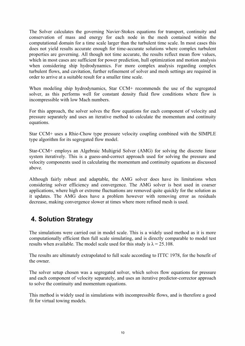
The model was setup as a transient solution. This was necessary in order to capture the free-surface effects, and multi-phase interface. The Implicit solver is the only choice for transient segregated solutions in Star CCM+. This allows the user to control the solution directly by defining the time step, and number if inner iterations used for each time step, both by specifying a constant value, and also by selecting criteria based convergence, where the solution will update and proceed when certain user selected properties are satisfied, such as forces, residuals, or motions. The SIMPLE algorithm was used in the Implicit approach. The SIMPLE algorithm progression is described in Figure 4.1.

Although this is a transient simulation, the desired results are mean values since this is effectively a speed and power prediction, therefore it is possible to maintain slightly higher Convective Courant values throughout the solution and progress the solution at a slightly more aggressive time step, while maintaining solution accuracy. The simulations are set up to simulate a virtual towing tank (VTT) simulation, in modified self-propulsion. The following solvers were enabled to solve the physical conditions of the flow and body forces.

Implicit Unsteady/Segregated Flow Eulerian Multiphase/Multiphase Mixture/Multiphase Equation of State Volume of Fluid (VOF) Gravity K-Omega (SST)

No motion solver was used in the simulations. The geometry was fixed in all six degrees of

Update Density

Correct Cell Velocities

Correct Mass Flux

Update Boundary Pressure Values

Update Pressure Field

Solve Pressure Correction Equ.

Compute Uncorrected Mass Fluxes

Solve Discrete Momentum Equ.

Compute Velocity and Pressure Gradients

Set Boundary Conditions

Start

Figure 4.1

11

freedom (6-DOF). This normally results in an under prediction of drag values. Accuracy in predicted total resistane (RT) values can be improved with the application of a motion solver. This topic will be discussed in more detail in section 6. 4.1 Assumptions and Simplifications

Only one of the models is based on an existing vessel so a suitable geometrical strategy was needed for the simulation setup. Since the intention of the study was to replicate actual conditions (as built) as much as possible, the hull and propulsion arrangement for the Norwegian Jewel (Meyer Hull 667) was selected. This vessel was outfitted with Azipods®for the propulsion arrangement and will serve as the control for the comparison (POD). All the information required for setting up a CFD simulation was available for this vessel. No sister vessel, outfitted with shaftlines was available for comparison so it was decided to use the same hull-form from Norwegian Jewel, and outfit it with shaftlines based on the hull-form from the Norwegian Spirit (ex. Superstar Leo, Meyer Hull 646) to serve as the comparison vessel (SHAFT). The vessel particulars are similar between these vessels with a difference in length of approx. 26m and a difference in draft of 0.3m. The propulsion arrangement including shaft alignment and rudder placement has been arranged according to the design particulars of the Norwegian Spirit. This vessel has open shaftlines, with full-spade rudders. 4.2 Geometry and Mesh Continua

Star CCM+ uses an auto meshing tool which employs two steps in order to arrive at a core finite volume mesh. Following importation and repair of CAD geometry, the mesh solver first produces a tetrahedral surface mesh based on the Octree method, followed by a volume mesh based on the previously created surface mesh. The mesh strategy used in this study is the same for both hull models. The mesh has been resolved using two regions; Domain and Disc. This has been done for the sake of the momentum source model, which requires a closed region located inside the domain representing the propeller disc. Internal interfaces are defined at the Disc boundaries to allow mass, energy and continua properties to pass between regions. A trimmed mesh was used, providing a predominately hexahedral mesh. The trimmer feature allows mesh alignment which proves very useful for simulations where the phase interface needs to be sharp, such as towing simulations where it is necessary to capture the effects of the free surface waves. The Domain size needs to be carefully chosen to ensure accuracy in results with reasonable computational speed. It is also important to consider the proper dissipation of wave energy as waves propagate away from the vessel. If the mesh transitions too quickly, or remains too refined as it approaches the boundaries, waves can reflect back towards the hull geometry causing oscillations in the drag values based on the waves hitting the hull. This becomes more important when the motion solver is active, as reflecting waves can cause the vessel to oscillate, or rock, causing inaccuracy in the solution and delayed convergence.

12

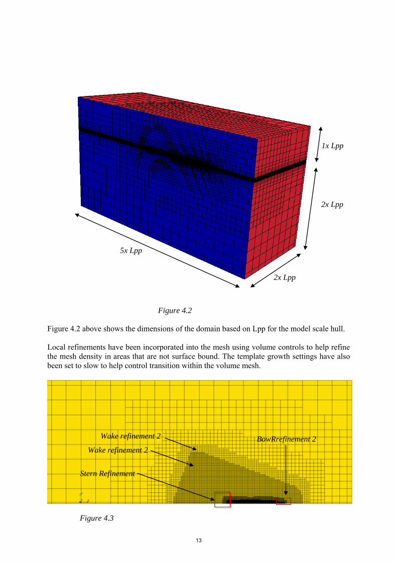
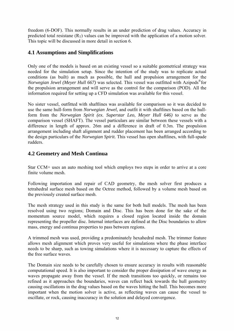
Figure 4.2 above shows the dimensions of the domain based on Lpp for the model scale hull. Local refinements have been incorporated into the mesh using volume controls to help refine the mesh density in areas that are not surface bound. The template growth settings have also been set to slow to help control transition within the volume mesh.

5x Lpp

2x Lpp

2x Lpp

1x Lpp

Stern Refinement

Wake refinement 2

Figure 4.3

BowRrefinement 2 Wake refinement 2

Figure 4.2

13

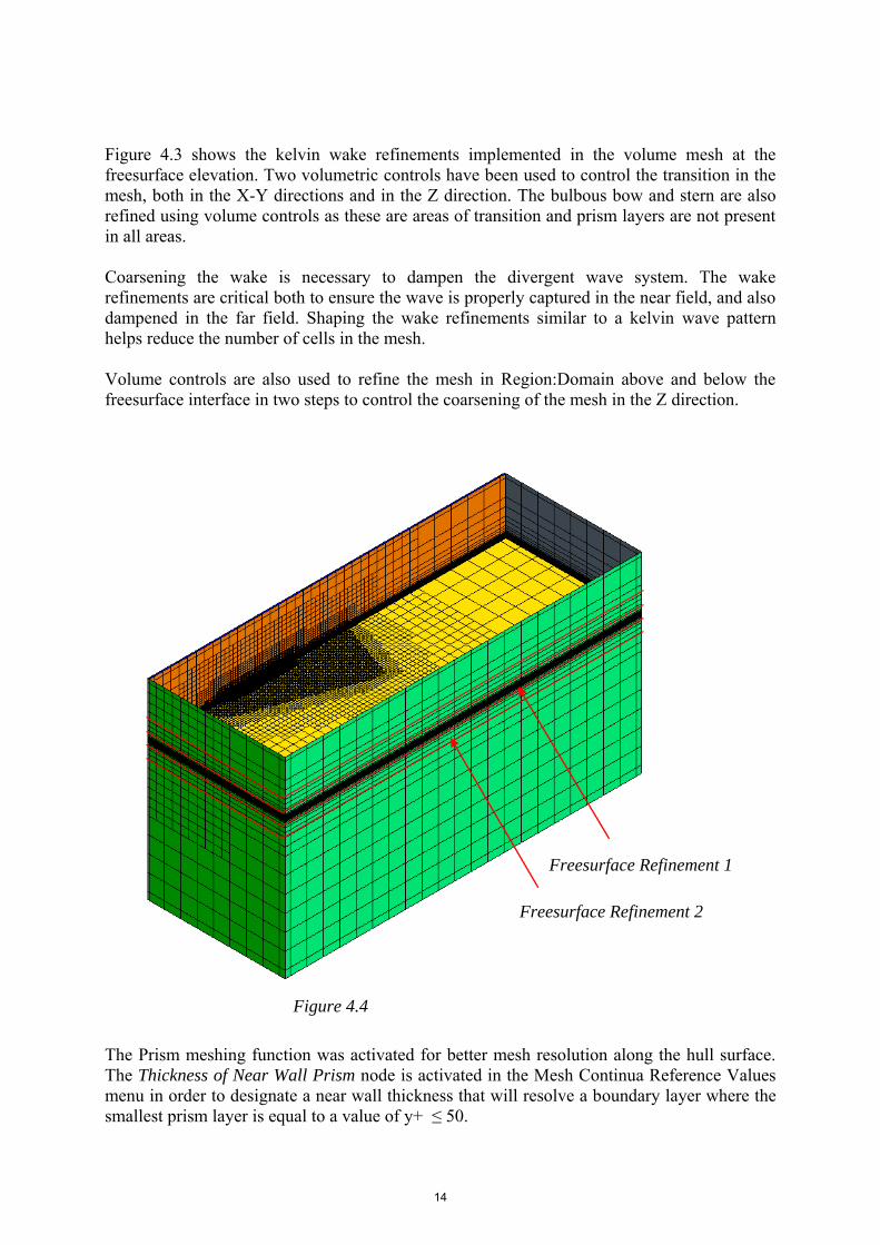
Figure 4.3 shows the kelvin wake refinements implemented in the volume mesh at the freesurface elevation. Two volumetric controls have been used to control the transition in the mesh, both in the X-Y directions and in the Z direction. The bulbous bow and stern are also refined using volume controls as these are areas of transition and prism layers are not present in all areas. Coarsening the wake is necessary to dampen the divergent wave system. The wake refinements are critical both to ensure the wave is properly captured in the near field, and also dampened in the far field. Shaping the wake refinements similar to a kelvin wave pattern helps reduce the number of cells in the mesh. Volume controls are also used to refine the mesh in Region:Domain above and below the freesurface interface in two steps to control the coarsening of the mesh in the Z direction.

The Prism meshing function was activated for better mesh resolution along the hull surface. The Thickness of Near Wall Prism node is activated in the Mesh Continua Reference Values menu in order to designate a near wall thickness that will resolve a boundary layer where the smallest prism layer is equal to a value of y+ ≤ 50.

Freesurface Refinement 1

Freesurface Refinement 2

Figure 4.4

14

y+ values are calculated based on:

and √

(4.1)

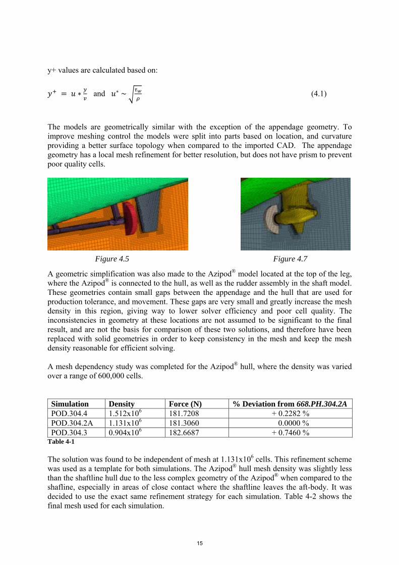
The models are geometrically similar with the exception of the appendage geometry. To improve meshing control the models were split into parts based on location, and curvature providing a better surface topology when compared to the imported CAD. The appendage geometry has a local mesh refinement for better resolution, but does not have prism to prevent poor quality cells.

A geometric simplification was also made to the Azipod® model located at the top of the leg, where the Azipod® is connected to the hull, as well as the rudder assembly in the shaft model. These geometries contain small gaps between the appendage and the hull that are used for production tolerance, and movement. These gaps are very small and greatly increase the mesh density in this region, giving way to lower solver efficiency and poor cell quality. The inconsistencies in geometry at these locations are not assumed to be significant to the final result, and are not the basis for comparison of these two solutions, and therefore have been replaced with solid geometries in order to keep consistency in the mesh and keep the mesh density reasonable for efficient solving. A mesh dependency study was completed for the Azipod® hull, where the density was varied over a range of 600,000 cells. Simulation Density Force (N) % Deviation from 668.PH.304.2A

POD.304.4 1.512x106 181.7208 + 0.2282 % POD.304.2A 1.131x106 181.3060 0.0000 % POD.304.3 0.904x106 182.6687 + 0.7460 %

Table 4-1

The solution was found to be independent of mesh at 1.131x106 cells. This refinement scheme was used as a template for both simulations. The Azipod® hull mesh density was slightly less than the shaftline hull due to the less complex geometry of the Azipod® when compared to the shafline, especially in areas of close contact where the shaftline leaves the aft-body. It was decided to use the exact same refinement strategy for each simulation. Table 4-2 shows the final mesh used for each simulation.

Figure 4.5 Figure 4.7

15

Simulation Density

POD.304.2A 1.131x106

SHAFT.304.2 1.512x106 Table 4-2

4.3 Physics Continua

Prior to selecting the physics quantities and initial conditions for each boundary, some global settings need to be established under the Physics Continua in the solver. 4.3.1 Physics Models

When simulating a multi-phase model, Star CCM+ requires the user to define the phases present in the model and their material properties. This is completed under the Eulerian Multiphase settings in the Physics Continua. For this study, Sea Water and Air at 20 C were selected. A convection scheme for the segregated flow model, k-ω (SST) turbulence model, and VOF model needs to be selected as well. For the sake of solution accuracy, 2nd order convection has been selected for all solver settings, with the exception of temporal discretization which remains 1st order for the sake of solver efficiency, as we are not looking for time accurate results. Under the VOF Wave settings, a VOF wave needs to be defined. This study does not cover sea-keeping properties, so a Flat VOF wave will be defined. The following conditions listed in Table 4-3 apply to both simulations as model scale: Flat VOF Wave 1 Point On Water Level (0,0,0.331)m Vertical Direction (0,0,1) Current (-2.443,0,0) m/s Wind (-2.443,0,0) m/s Light Fluid Density 1.18415 kg/m^3 Heavy Fluid Density 1025.9 kg/m^3

Table 4-3

Point on water level defines the point of phase interface. Wind and Current have been set equal to the design speed of the vessel at model scale, with Fn= 0.237. Under the VOF model settings, the user can define lower and upper limits for CFL numbers for the High Resolution Interface Capturing (HRIC) scheme. The HRIC scheme controls the convective transport of immiscible fluid components. The HRIC scheme is very important for transient simulations where the CFL number varies throughout the domain, and the time step is too large to resolve large variations in the freesurface shape. For these types of conditions, and also for steady state conditions, the HRIC scheme is the most suited. Settings were adjusted so that the CFLL value settings were lower than the maximum CFL number contained within the domain, so that HRIC was always used. This is applicable to these

16

simulations due to the more aggressive time step, where the time step is too large to capture the transient effects of the free surface at some points in the domain, even though the freesurface is significantly refined. For this study, the target value for CFL ≤ 1, however there are a few cells in the domain approaching CFL=5. In order to insure the HRIC scheme is used for capturing phase interface, parameters have been set to CFLL = 50 and CFLL = 100. 4.3.2 Governing Equations

Volume of Fluid (VOF) Model:

∑ ∑ ∑

(4.2)

Where ρ, μ, and Cp are the density, molecular viscosity, and specific heat of the ith phase. The Volume Fraction is then represented by:

(4.3) HRIC Scheme:

Where is the normalized face value, and is the normalized cell center:

{

(4.4)

The Normalized face is further corrected according to the local Courant (CFL) number:

(4.5)

Resulting in a corrected value, valid for transient simulations of:

{

(

(4.6)

17

The k-ω (SST) turbulence model is defined as:

∫ ∫ ( )

∫ ∫ (

) (4.7)

∫ ∫ ( )

∫ ∫ (

)

(4.8)

Where the Turbulent Kenetic Energy source term Gk is produced according to the standard k-

ω model and the Turbulent Dissipation source term Gω is defined as:

*(

)

+ (4.9)

4.3.3 Reference Values

The solver requires reference values for the gravity model, as well as definition of the reference pressure and a reference altitude. The reference pressure has been set to atmospheric pressure with the location at the still waterline. Gravity has been set to a value:

4.3.4 Initial Conditions

The initial conditions apply to initial values for each cell contained within the domain with the exception to boundary specific conditions which will be discussed in section 4.4. The required initial conditions are outlined in Table 4-4. Turbulence settings have been specified according to Intensity and Viscosity Ratio. It is also possible to define turbulence initial conditions according to k-ω values, or Intensity and Length Scale values. Physical Property Setting Value

Pressure Field Function Hydrostatic Pressure of Flat Wave Turbulence Intensity Constant 0.019 Turbulent Velocity Scale Constant 1.0 m/s Turbulent Viscosity Ratio (TVR) Constant 2.0 Velocity Field Function Velocity of Flat Wave Volume Fraction Composite Vol Fraction of Light Phase Vol Fraction of Heavy Phase

Table 4-4

18

Turbulence intensity has been calculated according to:

⁄ (4.10)

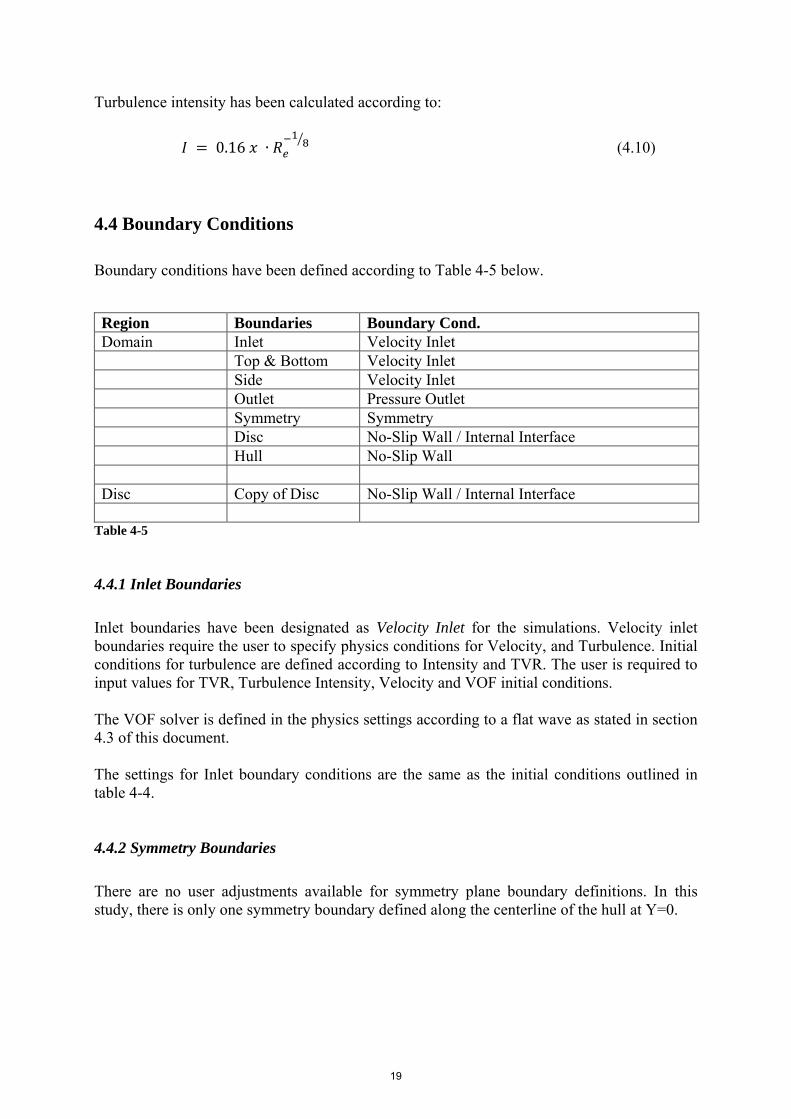
4.4 Boundary Conditions

Boundary conditions have been defined according to Table 4-5 below.

Region Boundaries Boundary Cond.

Domain Inlet Velocity Inlet Top & Bottom Velocity Inlet Side Velocity Inlet Outlet Pressure Outlet Symmetry Symmetry Disc No-Slip Wall / Internal Interface Hull No-Slip Wall Disc Copy of Disc No-Slip Wall / Internal Interface

Table 4-5

4.4.1 Inlet Boundaries

Inlet boundaries have been designated as Velocity Inlet for the simulations. Velocity inlet boundaries require the user to specify physics conditions for Velocity, and Turbulence. Initial conditions for turbulence are defined according to Intensity and TVR. The user is required to input values for TVR, Turbulence Intensity, Velocity and VOF initial conditions. The VOF solver is defined in the physics settings according to a flat wave as stated in section 4.3 of this document. The settings for Inlet boundary conditions are the same as the initial conditions outlined in table 4-4. 4.4.2 Symmetry Boundaries

There are no user adjustments available for symmetry plane boundary definitions. In this study, there is only one symmetry boundary defined along the centerline of the hull at Y=0.

19

4.4.3 Outlet Boundaries

Outlet boundaries have been designated as Pressure Outlet for the simulations. Pressure outlet boundaries require the user to specify physics conditions for Backflow Direction, Target Mass Flow, and Turbulence. Initial conditions for turbulence are defined according to Intensity and TVR. The user is required to input values for TVR, Turbulence Intensity, Pressure and VOF initial conditions. The VOF solver is defined in the physics settings according to a flat wave as stated in section 4.3 of this document. The settings for Inlet boundary conditions are the same as the initial conditions outlined in table 4-4. 4.4.4 Region Settings

With the application of the momentum source model, region settings pertaining to each region will need to be defined separately. The user has the option to specify motion settings, turbulence source parameters, and momentum source criteria. Star-CCM+ also allows the option to activate a VOF wave dampening function. This is a useful function when motion analysis is also being solved, however it has not been used in this study since the vessels have been fixed in all 6-DOF. The following region settings apply:

Region: Domain will not have any motion or momentum source models defined. Region: Disc will define a momentum source according to a set or user defined field functions and field reports.

4.4.5 Momentum Source Model

The momentum source model is defined as a vector profile. In this study the momentum source is generated based on the instantaneous drag for each time step as the solution progresses via a field report and field monitor. The momentum source has been defined according to the following: A force report is defined to tabulate the force exerted on the hull by the wind and current in the X-direction.

[FxReport] (4.11) A sum report is defined to calculate the volume of the Disc domain:

[VolCylReport] (4.12) An expression report is defined:

20

Momsource = [(Time <2)?0 :$DragReport/$VolCylReport] (4.13)

to calculate the momentum, as well as control the initialization of the momentum source model. This expression states that when time < 2 sec, the momentum source will be 0, after which it will be equal to the drag force distributed over the volume of the cylinder. A field function is defined: [-MomsourceReport,0,0] (4.14) and is used as the definition for the momentum source under the region settings for the Region:Disc. Unfortunately no vorticity, or swirl, is modelled in the propeller slip-stream which leads to inaccuracy in hull pressure around the propeller, however it is a reasonable approximation of the propeller induced drag on the appendages which is important to this study. 4.5 Solver

The solvers settings have largely been kept to the default values. The time step (ts) has been calculated so CFL ≤ 1.0. The CLF number was calculated according to:

CFL = U∆t/∆x 1.0 (4.15)

where U = free stream velocity, ∆t is the time step, and ∆x is the length of the smallest cell in the mesh. Under-Relaxation values have been kept at default, as well as Algebraic Multigrid (AMG) solver settings. Stopping criteria has been set to advance the solution at ts = 0.05s after five inner iterations have been completed. Stopping criteria is based on experience from previous virtual towing tank simulations (VTT) where mean flow values are the captured.

21

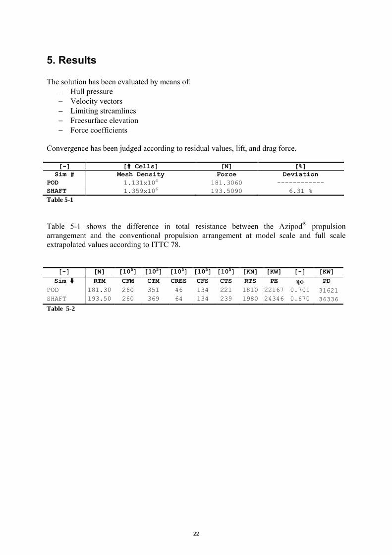
5. Results The solution has been evaluated by means of:

Hull pressure Velocity vectors Limiting streamlines Freesurface elevation Force coefficients

Convergence has been judged according to residual values, lift, and drag force.

[-] [# Cells] [N] [%]

Sim # Mesh Density Force Deviation

POD 1.131x106 181.3060 ------------

SHAFT 1.359x106

193.5090 6.31 %

Table 5-1

Table 5-1 shows the difference in total resistance between the Azipod® propulsion arrangement and the conventional propulsion arrangement at model scale and full scale extrapolated values according to ITTC 78.

[-] [N] [105] [105] [105] [105] [105] [KN] [KW] [-] [KW]

Sim # RTM CFM CTM CRES CFS CTS RTS PE ηo PD

POD 181.30 260 351 46 134 221 1810 22167 0.701 31621

SHAFT 193.50 260 369 64 134 239 1980 24346 0.670 36336

Table 5-2

22

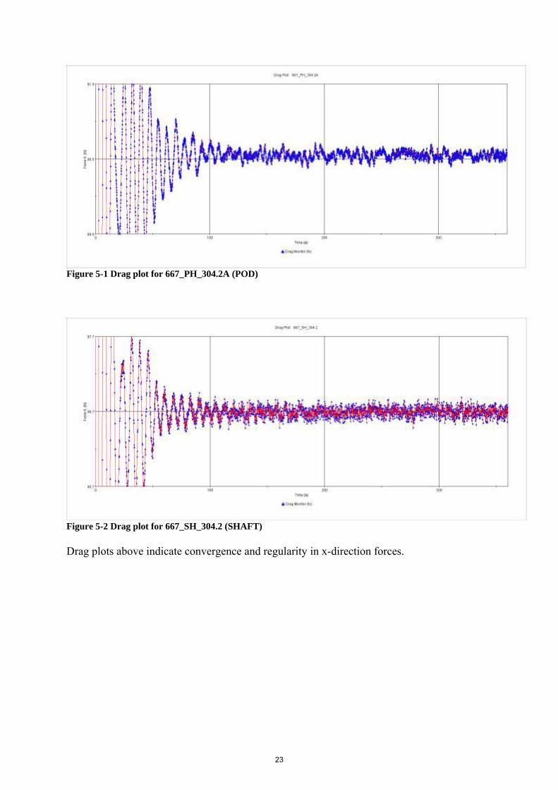
Figure 5-1 Drag plot for 667_PH_304.2A (POD)

Figure 5-2 Drag plot for 667_SH_304.2 (SHAFT)

Drag plots above indicate convergence and regularity in x-direction forces.

23

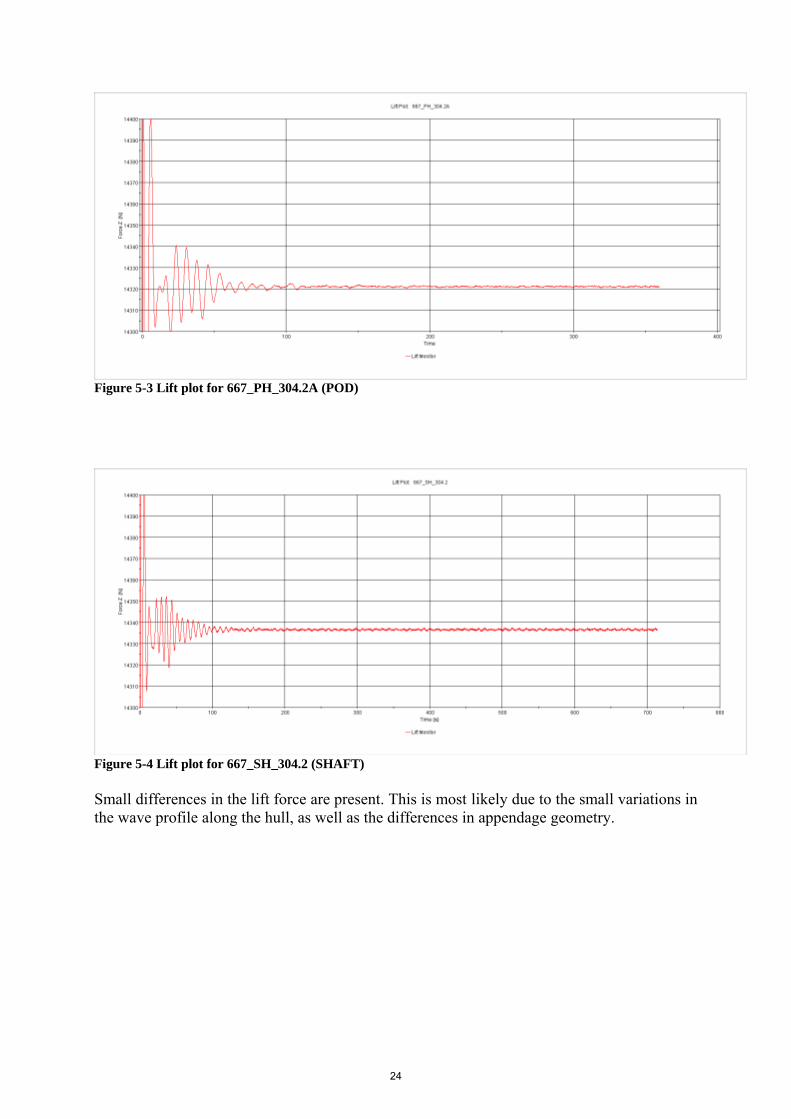
Figure 5-3 Lift plot for 667_PH_304.2A (POD)

Figure 5-4 Lift plot for 667_SH_304.2 (SHAFT)

Small differences in the lift force are present. This is most likely due to the small variations in the wave profile along the hull, as well as the differences in appendage geometry.

24

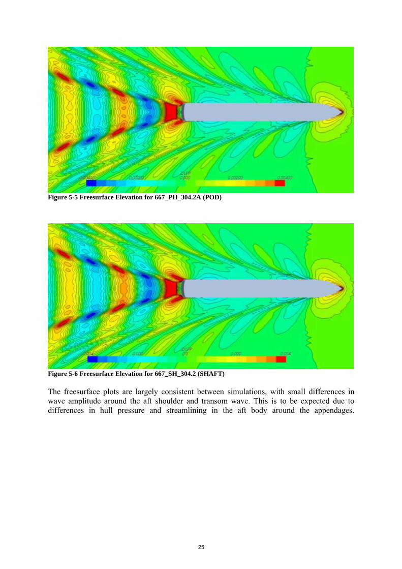
Figure 5-5 Freesurface Elevation for 667_PH_304.2A (POD)

Figure 5-6 Freesurface Elevation for 667_SH_304.2 (SHAFT)

The freesurface plots are largely consistent between simulations, with small differences in wave amplitude around the aft shoulder and transom wave. This is to be expected due to differences in hull pressure and streamlining in the aft body around the appendages.

25

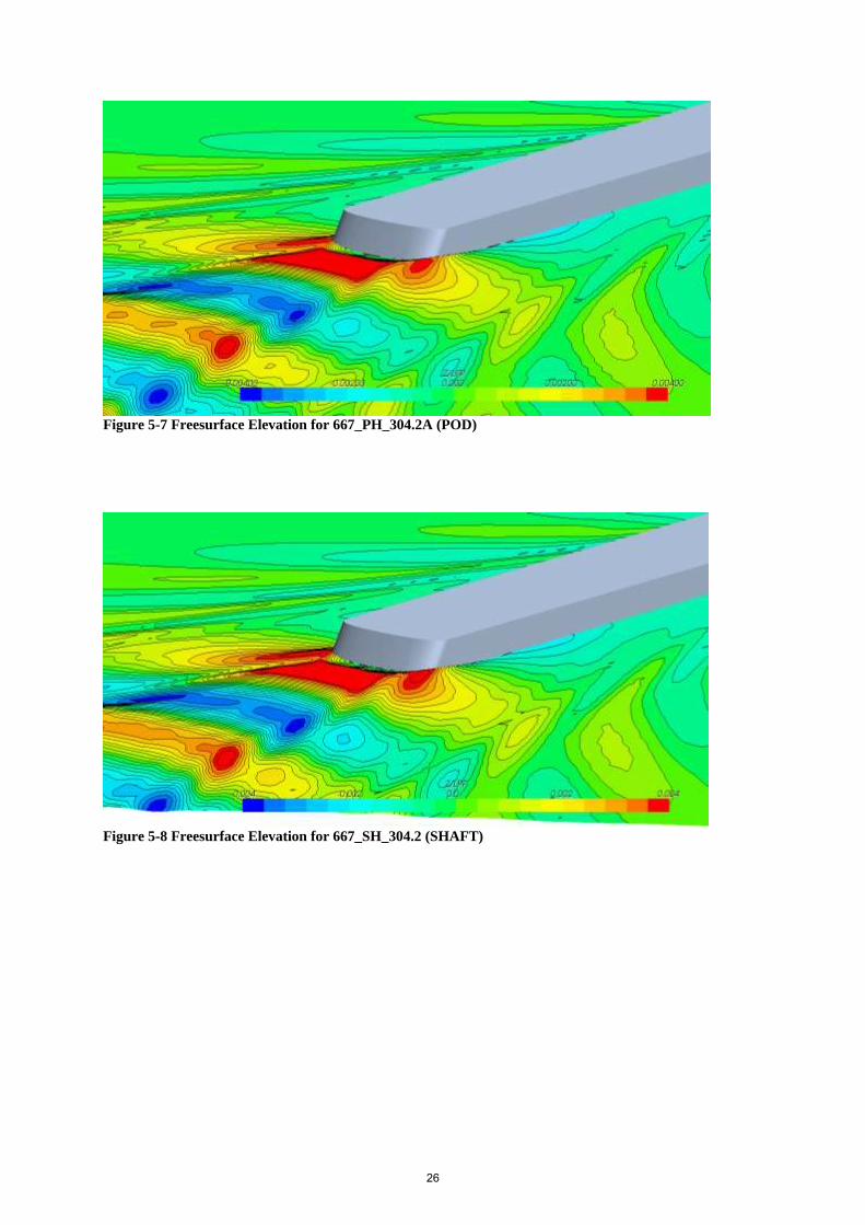
Figure 5-7 Freesurface Elevation for 667_PH_304.2A (POD)

Figure 5-8 Freesurface Elevation for 667_SH_304.2 (SHAFT)

26

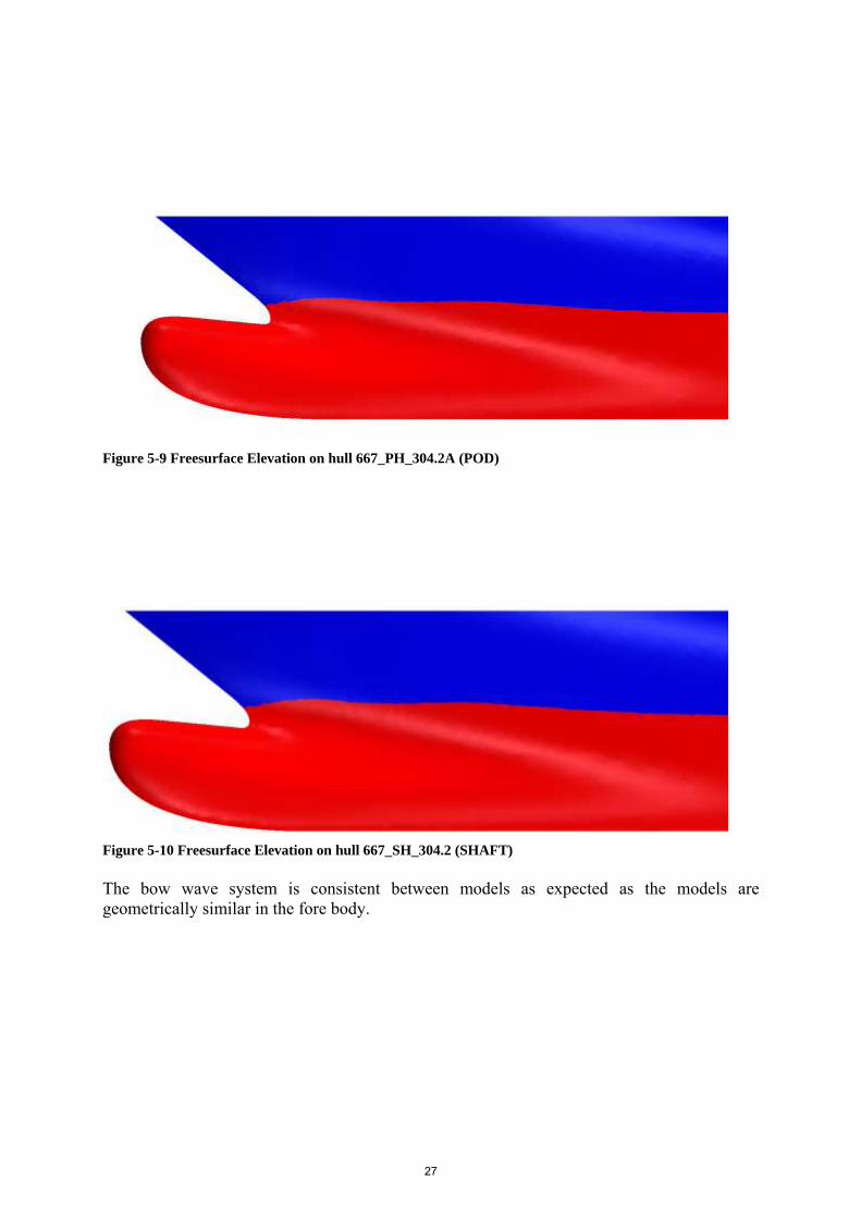
Figure 5-9 Freesurface Elevation on hull 667_PH_304.2A (POD)

Figure 5-10 Freesurface Elevation on hull 667_SH_304.2 (SHAFT)

The bow wave system is consistent between models as expected as the models are geometrically similar in the fore body.

27

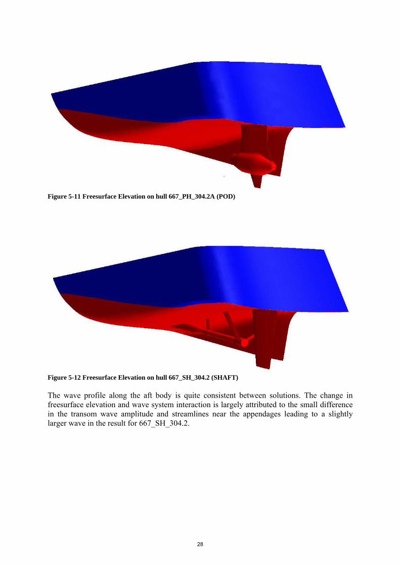
Figure 5-11 Freesurface Elevation on hull 667_PH_304.2A (POD)

Figure 5-12 Freesurface Elevation on hull 667_SH_304.2 (SHAFT)

The wave profile along the aft body is quite consistent between solutions. The change in freesurface elevation and wave system interaction is largely attributed to the small difference in the transom wave amplitude and streamlines near the appendages leading to a slightly larger wave in the result for 667_SH_304.2.

28

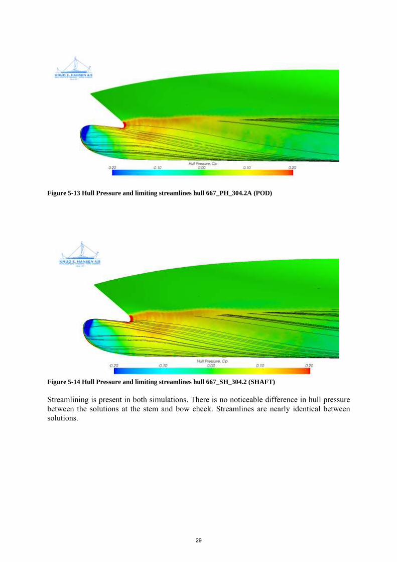
Figure 5-13 Hull Pressure and limiting streamlines hull 667_PH_304.2A (POD)

Figure 5-14 Hull Pressure and limiting streamlines hull 667_SH_304.2 (SHAFT)

Streamlining is present in both simulations. There is no noticeable difference in hull pressure between the solutions at the stem and bow cheek. Streamlines are nearly identical between solutions.

29

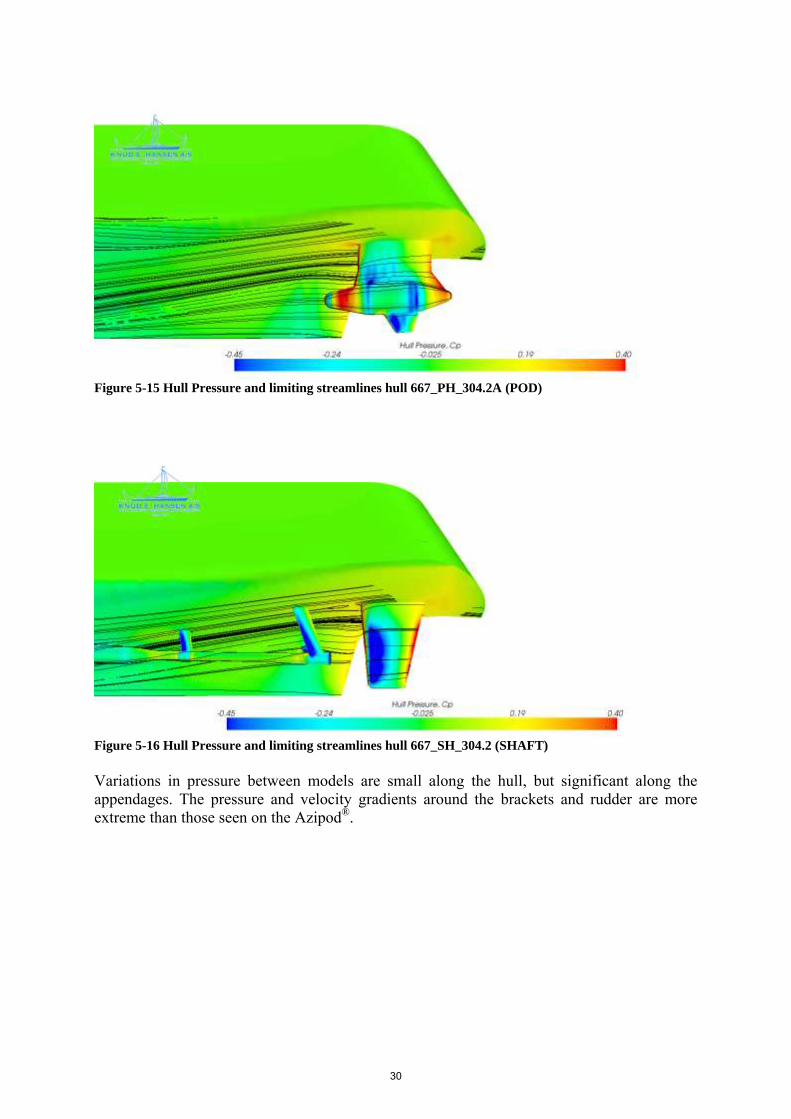
Figure 5-15 Hull Pressure and limiting streamlines hull 667_PH_304.2A (POD)

Figure 5-16 Hull Pressure and limiting streamlines hull 667_SH_304.2 (SHAFT)

Variations in pressure between models are small along the hull, but significant along the appendages. The pressure and velocity gradients around the brackets and rudder are more extreme than those seen on the Azipod®.

30

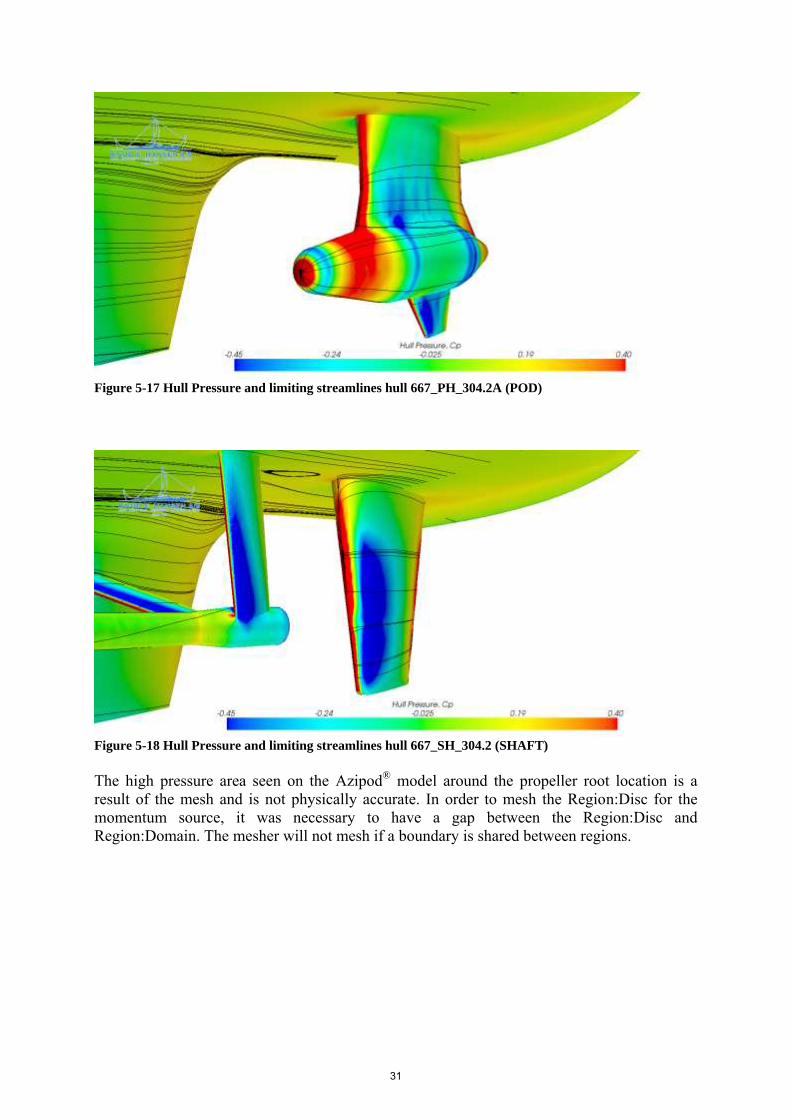
Figure 5-17 Hull Pressure and limiting streamlines hull 667_PH_304.2A (POD)

Figure 5-18 Hull Pressure and limiting streamlines hull 667_SH_304.2 (SHAFT)

The high pressure area seen on the Azipod® model around the propeller root location is a result of the mesh and is not physically accurate. In order to mesh the Region:Disc for the momentum source, it was necessary to have a gap between the Region:Disc and Region:Domain. The mesher will not mesh if a boundary is shared between regions.

31

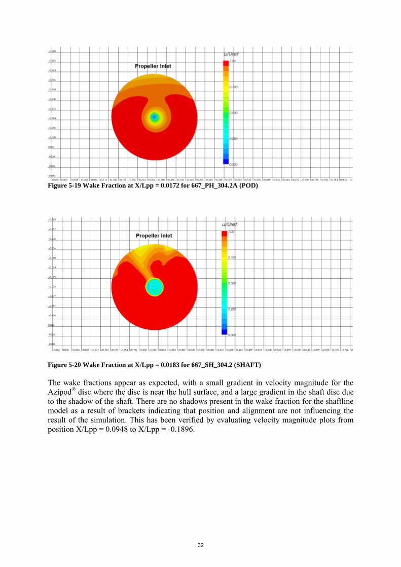
Figure 5-19 Wake Fraction at X/Lpp = 0.0172 for 667_PH_304.2A (POD)

Figure 5-20 Wake Fraction at X/Lpp = 0.0183 for 667_SH_304.2 (SHAFT)

The wake fractions appear as expected, with a small gradient in velocity magnitude for the Azipod® disc where the disc is near the hull surface, and a large gradient in the shaft disc due to the shadow of the shaft. There are no shadows present in the wake fraction for the shaftline model as a result of brackets indicating that position and alignment are not influencing the result of the simulation. This has been verified by evaluating velocity magnitude plots from position X/Lpp = 0.0948 to X/Lpp = -0.1896.

32

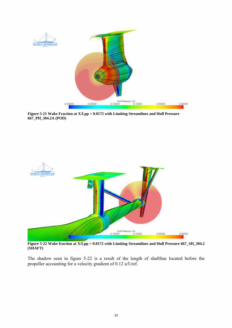
Figure 5-21 Wake Fraction at X/Lpp = 0.0172 with Limiting Streamlines and Hull Pressure

667_PH_304.2A (POD)

Figure 5-22 Wake fraction at X/Lpp = 0.0172 with Limiting Streamlines and Hull Pressure 667_SH_304.2

(SHAFT)

The shadow seen in figure 5-22 is a result of the length of shaftline located before the propeller accounting for a velocity gradient of 0.12 u/Uref.

33

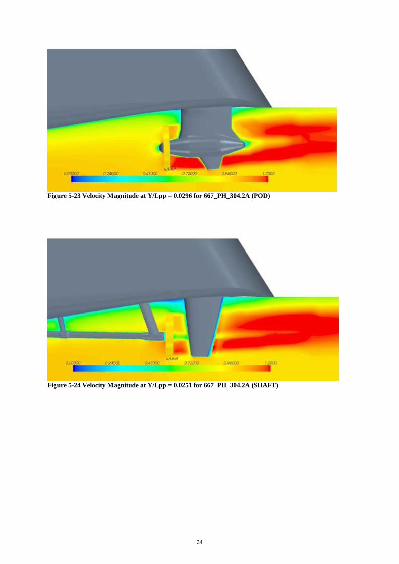
Figure 5-23 Velocity Magnitude at Y/Lpp = 0.0296 for 667_PH_304.2A (POD)

Figure 5-24 Velocity Magnitude at Y/Lpp = 0.0251 for 667_PH_304.2A (SHAFT)

34

6. Conclusion Since the models are geometrically similar in all ways apart from the appendages, there are no noticeable differences in residuary resistance, making viscous resistance the dominating factor. The simulation results indicate considerable differences in terms of total drag, and propulsive efficiency attributed largely to the increase in turbulence around the shaftline and brackets and the increase in wetted surface of approximately 1.4% on the shaftline vessel. The shaftlines cause a considerable velocity gradient at the inlet to the propeller, resulting in necessary changes to propeller design to account for uneven loading on the blades as they pass in and out of the shadow. As a result, propeller efficiency is lower in the shaftline solution, increasing the Delivered Power (PD) requirement. Result accuracy can be improved by capturing the dynamic motions of the hull in the fluid by implementing the Dynamic Fluid Body Interaction (DFBI) solver and adding further refinement to the multiphase interface to try to better capture the wave breaking effects and spray in the near field. Substitution of the momentum source model with the actual propeller geometry will add accuracy when calculating hull pressure through better resolution of turbulence and cavitation effects in the aft body due to propeller action. Discussion can be made around the method used in selecting the models and appendage arrangements since the POD model is based on an existing vessel and the SHAFT model is based on the best estimate from a similar hull geometry in an earlier vessel series. The justification for this approach relies heavily on controlling the amount of change from one hull version to the other. There are more changes to consider aside from obvious changes to the underwater geometry. By changing the hull shape, it can be assumed that the internal compartmentalization will be changed as well, including machinery spaces and public spaces. Change to internal space drives cost and revenue onboard a cruise vessel. Changing the space definition may result in a negative impact on the number of lower berths onboard, or revenue generating public spaces, making the vessel less profitable, despite possible gains in hydrodynamics. The purpose of this study was to evaluate two similar hull forms on a common building platform in order to make an economic comparison based on the difference in hydrodynamic efficiency, and avoid introducing additional areas of uncertainty in regards to Total Cost of Ownership (TCO) or operating costs. With this in mind, it was decided that the hull shape would remain constant for all simulations, insuring that displacement, lightweight, and deadweight would remain constant, and the subdivision and space definition, including all spaces in the superstructure would remain unchanged.

35

9. References Jurgens, D., Palm, M., Peric, M., and Schreck, E., Prediction of Resistance of Floating Vessels, March 2008. Xing,T., Carrica, P., and Stern, F., Computational Towing Tank Procedures for Single Run Curves of Resistance and Propulsion, Vol. 130, October 2008. Brizzolara, S., and Serra, S., Accuracy of CFD Codes in the Prediction of Planing Surfaces Hydrodynamic Characteristics, Univeristy of Genoa, Department of Naval Architecture and Marine Technology, June 2007. Buncan, B., Buca, M.P, Ruzic, S., Numerical Modelling of the Flow Around the Tanker Hull at Model Scale, Numerical Hydrodynamics Deptartment, Ship Hydrodynamics, Brodarski Institut. Croatia, May 2008. Thornhill, E., Oldford, D., Bose, N., Veitch, B., Liu, P., Planing Hull Model Test for CFD Validation, 6th Canadian Marine Hydromechanics and Structures Conference, Vancoucer, BC Canada, 2001. Versteeg H.K. & Malalasekera W., An introduction to computational fluid dynamics – the finite volume method, Addison Wesley Longman Limited, 1995, ISBN 0-582-21884-5. Vanderplaats, G. N., Numerical optimization techniques for engineering design., 3rd Edition, Fourth Printing, 2001. Star CCM+ user guide, 2011, CD-Adapco. Bensow R., Knud E. Hansen A/S, personal communication, 2006-2011. Luhmann, Henning, Knud E. Hansen A/S, personal communication, 2006-2011. Veikonheimo, Tomi, Knud E. Hansen A/S, personal communication, 2006-2011. ITTC Recommended Procedures – Process Control – CFD 7.5-03, Rev 4, 2008. <http://ittc.sname.org/new%20recomendations/pdf%20Procedures%202008/register.pdf> Umlauf, L., and Burchard, H., A generic length-scale equation for goephysical turbulence models, Journal of Marine Research, 61, 235-265, 2003. Chou, S.K., Hsin, C.Y., Chen, W.C., and Chau, S.W., Simulating the self-propulsion test by a coupled voscous/potential flow computation, August 2003.

36