“

”Advanced Automatic Control

If you have a smart project, you can say "I'm an engineer"

Lecture 3Staff boarder

Prof. Dr. Mostafa Zaki Zahran

Dr. Mostafa Elsayed Abdelmonem

Advanced Automatic Control

MDP 444

• Lecture aims:

• Facilitate combining and manipulating differential equations

• Identify the equations of motion of systems

• Understand the mathematical modeling of all systems and combination

Modeling of electrical system

• Kirchhoff ’s laws:

1. Kirchhoff ’s voltage law. The algebraic sum of the voltages in a loop is

equal to zero.

2. Kirchhoff ’s current law. The algebraic sum of the currents in a node is

equal to zero.

Modeling of electrical system

• Kirchhoff ’s laws:

Kirchhoff ’s voltage law. The algebraic sum of the voltages in a loop is equal to zero.

• Loop (1)

• V(t)= VR + Vc

• Loop (2)

• 0=VR + Vc

Modeling of electrical system

• Transfer from time domain to frequency domain:

• Transfer function

Modeling of electrical system

• Analogous to Kirchhoff ’s

laws for networks is

d’Alembert’s law for

mechanical systems which

is stated as follows:

D’Alembert’s law of forces:

The sum of all forces

acting upon a point mass is

equal to zero.

Element Physical variable Linear operator Inverse operator

Electrical Networks

Resistor RVoltage v(t)

Current i(t)Inductor L

Capacitor C

Mechanical Systems

Friction coefficient B Force f(t)

Velocity v(t)Mass m

Spring constant K

Mathematical Modeling Of Electronic

Circuits

• Operational amplifiers, often called op-amps, are important building blocks in

modem electronic systems. They are used in filters in control systems and to

amplify signals in sensor circuits.

• The input e1 to the minus terminal of the amplifier is inverted; the input e2

to the plus terminal is not inverted.)

Mathematical Modeling Of Electronic

Circuits

• Let us obtain the voltage ratio eo/ei. In the derivation, we assume the voltage at the minus terminal as e‘. This is called an imaginary short. Consider again the amplifier system

• e' = 0. Hence, we have

Mathematical Modeling Of Electronic

Circuits

• Obtain the relationship between the output eo and the inputs e1, e2, and e3

• e' = 0. Hence, we have

L

L

L

TTdt

dTRC

R

TT

dt

dTC

dt

dTCq

dt

dTCqq

R

TTq

;21

resistance thermal theis

ecapacitanc theis

flowheat of ratenet theis

R

C

q

qT

TL

Modeling of Thermal System

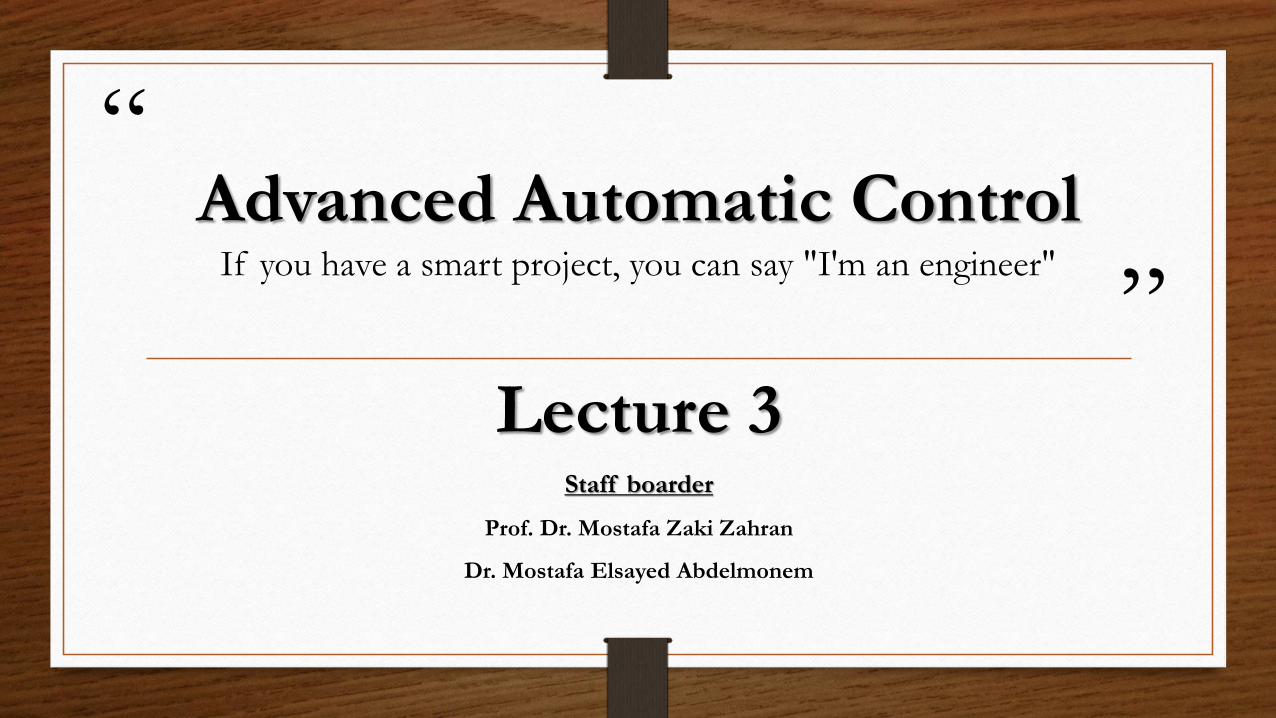
Mathematical Modeling Of A Thermal System

• Input – output = stored

qo = KΔθ

• The coefficient K is given by

𝑞𝑖 𝑡 − 𝑞𝑜 𝑡 = 𝑞𝑠𝑡𝑜𝑟𝑒𝑑

𝑞𝑠𝑡𝑜𝑟𝑒𝑑 = 𝑐𝑑𝜃(𝑡)

𝑑𝑡

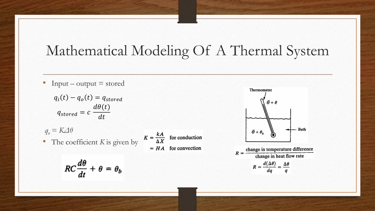
Modeling of Motors

s( )

V f s( )

K m

s J s b( ) L f s R f s( )

V a s( )

K m

s R a L a s J s b( ) K b K m

Modeling of Motors

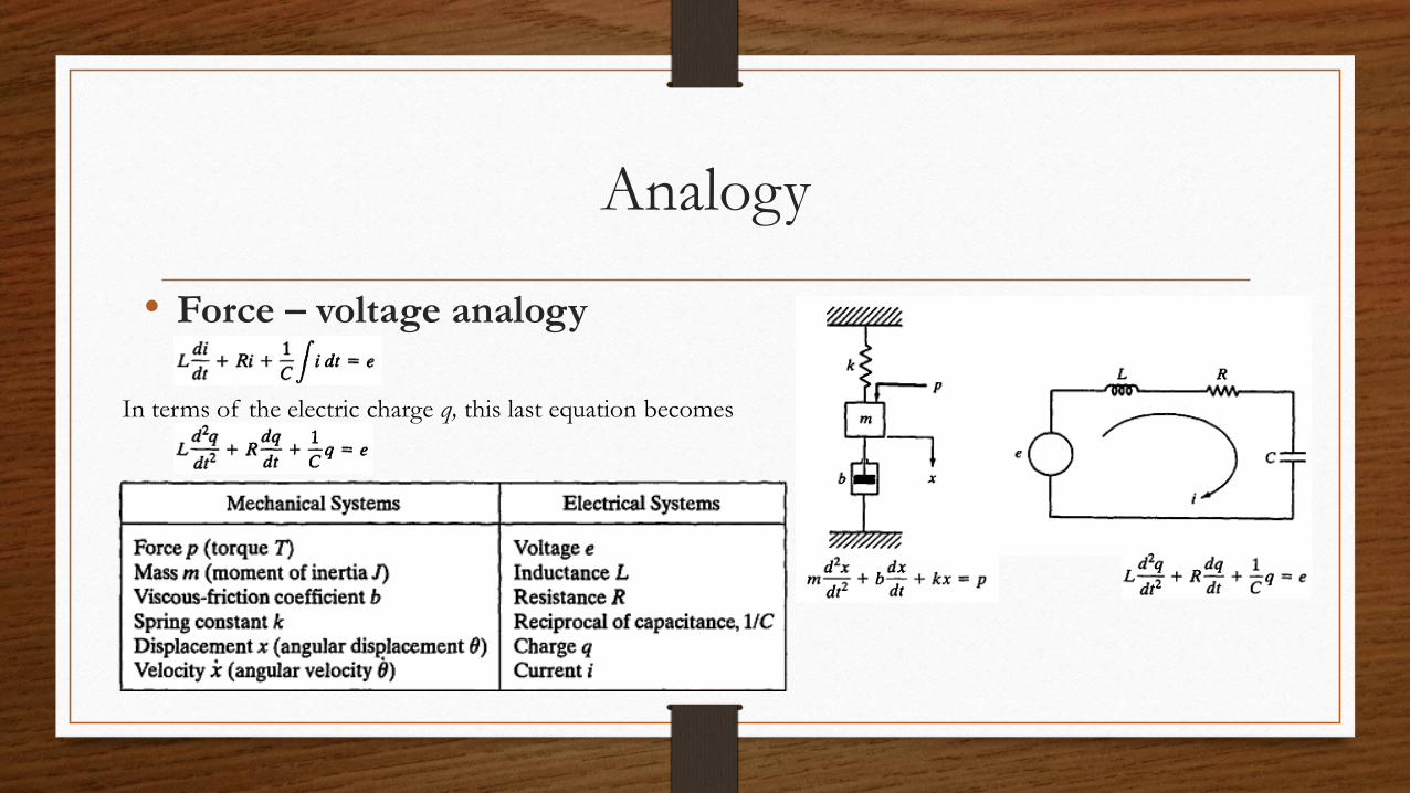
Analogy

• Force – voltage analogy

In terms of the electric charge q, this last equation becomes

Analogy

• Force – current analogy

In terms of the magnetic flux ψ, this last equation becomes

Modeling of Motors

Modeling of Motors

Modeling of Motors

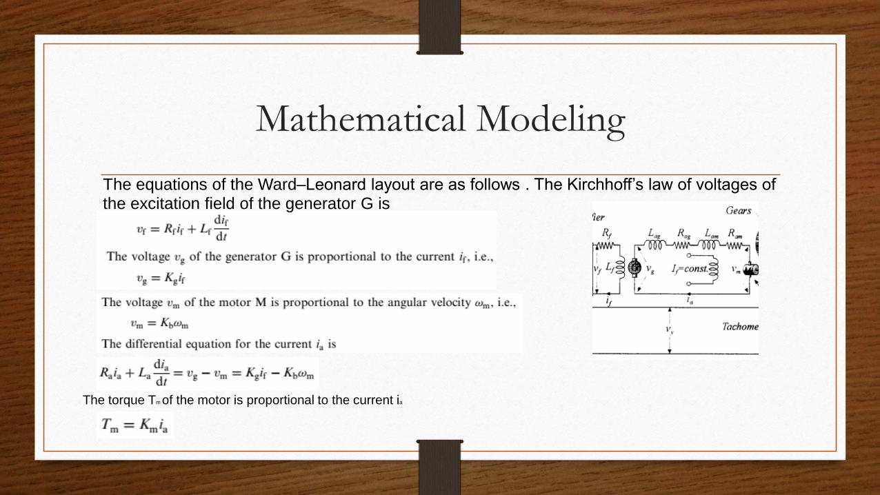
Mathematical Modeling

The torque Tm of the motor is proportional to the current ia

The equations of the Ward–Leonard layout are as follows . The Kirchhoff’s law of voltages of the excitation field of the generator G is

Mathematical Modeling

The equations of the Ward–Leonard layout are as follows . The Kirchhoff’s law of voltages of the excitation field of the generator G is

where use was made of the relation

The tachometer equation

the amplifier equation

𝑣𝑓 = 𝐾𝑎𝑣𝑒

where Jm *= Jm + N2JL and Bm * =Bm + N2 BL, where N = N1/N2.

Here, Jm is the moment of inertia and Bm the viscosity coefficient of the motor: likewise, for JL and BL of the load.

Mathematical Modeling

The mathematical model of the Ward–Leonard layout are as follows .

Ω𝑦(𝑠)

𝑣𝑒(𝑠)=

Analogy

• Force – voltage analogy

In terms of the electric charge q, this last equation becomes

Analogy

• Force – current analogy

In terms of the magnetic flux ψ, this last equation becomes

Model Examples

• Stepper motor